boast-nfr user's guide library/research/oil-gas/enhanced oil... · options for shape factors...
TRANSCRIPT

User’s Guide and Documentation Manual For BOAST-NFR For Excel
Prepared By
Jose G. Almengor, Gherson Penuela, Michael L. Wiggins, Raymon L. Brown, Faruk Civan, and Richard G. Hughes
Mewbourne School of Petroleum and Geological Engineering
The University of Oklahoma 100 East Boyd, Suite T-301 Norman, Oklahoma 73019
December 2002
DE-AC26-99BC15212
The University of Oklahoma Office of Research Administration
1000 Asp Avenue, Suite 314 Norman, Oklahoma 73019

BOAST-NFR User's Guide i
Table of Contents Page
Table of Contents................................................................................................................. i List of Tables ...................................................................................................................... ii List of Figures ..................................................................................................................... ii BOAST-NFR ...................................................................................................................... 1 1. Introduction..................................................................................................................... 2
1.1 Background............................................................................................................... 2 1.2 Mechanics of Simulation .......................................................................................... 2 1.3 Black-Oil Simulators ................................................................................................ 3
2. BOAST-NFR .................................................................................................................. 4 2.1 Model Overview ....................................................................................................... 4 2.2 Model Features.......................................................................................................... 5 2.3 Dynamic Redimensioning......................................................................................... 5 2.4 Restart Capabilities ................................................................................................... 6 2.5 Program Limitations ................................................................................................. 6 2.6 Restart Limitations.................................................................................................... 6
3. Getting Started with BOAST-NFR................................................................................. 8 3.1 Minimum Requirements ........................................................................................... 8 3.2 Simulation Run ......................................................................................................... 8 3.3 Loading the BOAST-NFR Program ......................................................................... 8 3.4 Data Input Requirements .......................................................................................... 9 3.5 Data Input Conventions .......................................................................................... 10 3.6 Running the BOAST-NFR Program....................................................................... 10
4. Data Initialization.......................................................................................................... 12 4.1 Introduction............................................................................................................. 12 4.2 Preparing the Input Data Spreadsheet..................................................................... 12
4.2.1 Grid Dimensions and Geometry ...................................................................... 12 4.2.2 Elevations to Top of Reservoir ........................................................................ 15 4.2.3 Porosity and Permeability Distributions .......................................................... 16 4.2.4 Inter-Porosity Flow Model............................................................................... 21 4.2.5 Faults................................................................................................................ 22 4.2.6 Relative Permeabilities and Capillary Pressures.............................................. 22 4.2.7 Rock-Fluid Properties at the Fracture/Matrix Interface................................... 24 4.2.8 Rock Compressibilities .................................................................................... 24 4.2.9 PVT Data ......................................................................................................... 25 4.2.10 Oil PVT Data ................................................................................................. 26 4.2.11 Water PVT Data............................................................................................. 26 4.2.12 Gas PVT Data ................................................................................................ 27 4.2.13 Fluid Densities ............................................................................................... 27 4.2.14 Pressure and Saturation Initialization ............................................................ 28 4.2.15 Run Control Parameters................................................................................. 30
4.2.16 Solution Method Control Parameters................................................................. 31 5. Recurrent Data .............................................................................................................. 33
5.1 Introduction............................................................................................................. 33 5.2 Timestep and Output Control Codes....................................................................... 33
BOAST-NFR User's Guide ii
5.3 Well Information Records....................................................................................... 35 5.3.1 Vertical Well Information................................................................................ 35 5.3.2 Horizontal Well Information............................................................................ 39 5.3.3 Slanted Well Information................................................................................. 40
6. Interpretation of Model Output..................................................................................... 44 6.1 Output Data Spreadsheet......................................................................................... 44
6.1.1 Material Balance Report .................................................................................. 44 6.1.2 Well Report...................................................................................................... 44 6.1.3 Summary Report in the Output Data Spreadsheet ........................................... 45 6.1.4 Variable Distribution Arrays............................................................................ 45
6.2 Summary Report Spreadsheet................................................................................. 46 6.3 Restart Data Spreadsheet ........................................................................................ 47
7. Example Input and Output Data ................................................................................... 48 7.1 Introduction............................................................................................................. 48 7.2 Problem Description ............................................................................................... 48 7.3 Input Data................................................................................................................ 52 7.4 Output Data............................................................................................................. 55 7.5 Summary Report ..................................................................................................... 57
8. References..................................................................................................................... 58
List of Tables Page
Table 4.1. Options for gridblock geometry....................................................................... 14 Table 4.2. Options for gridblock properties for the matrix system................................... 19 Table 4.3. Options for gridblock properties for the fracture system................................. 20 Table 4.4. Options for shape factors. ................................................................................ 21 Table 4.5. Options for repressurization algorithm. ........................................................... 25 Table 4.6. Pressure and saturation initialization codes ..................................................... 28 Table 5.1. Options for controlling well performance. ...................................................... 38 Table 7.1. Gridblock and reservoir rock basic data .......................................................... 48 Table 7.2. Fluid-rock properties in the matrix system...................................................... 49 Table 7.3. Undersaturated oil properties........................................................................... 50 Table 7.4. Saturated oil properties .................................................................................... 50
List of Figures Page
Figure 3.1. Starting up BOAST-NFR in Windows............................................................. 9 Figure 4.1. Number of gridblocks and switch codes. ....................................................... 12 Figure 4.2. Codes and dimensions for gridblocks............................................................. 13 Figure 4.3. Order of input when KDX is 0 for nx = 5 gridblocks in the x-direction. ....... 13 Figure 4.4. Order of input when KDY is 0 for ny = 4 gridblocks in the y-direction. ....... 14 Figure 4.5. Order of input when KDZ is 0 for nz = 3 gridblocks in the z-direction. ........ 15 Figure 4.6. Input data for grid dimensions when KDX, KDY, and KDZ are 0, for nx=5,
ny=4, and nz=3. ........................................................................................................ 15

BOAST-NFR User's Guide iii
Figure 4.7. Code and value for elevation from datum to top of sand. .............................. 15 Figure 4.8. Input data order for elevation in a 5x4x3 grid system. Distances measured
below the datum defined by the user. ....................................................................... 16 Figure 4.9. Porosity and permeability distributions for the matrix system....................... 17 Figure 4.10. Full permeability tensor................................................................................ 21 Figure 4.11. Porosity and permeability distributions for the fracture system. Fracture
permeability is modeled with a diagonal permeability tensor in this example......... 21 Figure 4.12. Default values used where there are no faults in the reservoir..................... 22 Figure 4.13. Location of a sealing fault in gridblock (2,4,1). Two segments are used to
represent the fault. These segments are no-flow boundaries (zero horizontal transmissibility)......................................................................................................... 22
Figure 4.14. Representation of the fault shown in Fig. 4.13............................................. 22 Figure 4.15. Relative permeability and capillary functions for the matrix system........... 23 Figure 4.16. Fracture system relative permeability and capillary functions..................... 24 Figure 4.17. Rock-fluid properties at the interface. .......................................................... 24 Figure 4.18. Rock compressibility for matrix and fracture systems as function of pressure.
................................................................................................................................... 24 Figure 4.19. PVT input data.............................................................................................. 25 Figure 4.20. Oil PVT data. The value next to the header is equal to the number of
pressure values in table (11 in this case)................................................................... 26 Figure 4.21. Water PVT data. The value next to the header is equal to the number
pressure values (2 in this case).................................................................................. 27 Figure 4.22. Gas PVT data. The value next to the header is equal to the number of
pressure values (11 in this case)................................................................................ 27 Figure 4.23. Oil, water, and gas phase densities in lb/cu ft. ............................................. 28 Figure 4.24. Pressure and saturation initialization for matrix system............................... 29 Figure 4.26. Run control parameters................................................................................ 30 Figure 4.27. Parameters controlling the LSOR solution method...................................... 32 Figure 5.1. Recurrent data pair for timestep and output control. ...................................... 34 Figure 5.2. Well information records showing one vertical producing well. ................... 35 Figure 5.3. Well information records showing a horizontal well. .................................... 40 Figure 5.4. Side view showing angle theta. ...................................................................... 41 Figure 5.5. Top view of grid showing angle alpha. .......................................................... 41 Figure 5.6. Well information records showing a slanted well with IFLAG = 1. .............. 42 Figure 5.7. Well information records showing a slanted well with IFLAG = 2. .............. 42 Figure 5.8. Side view of a slanted wellbore showing position in x-z plane. ..................... 43 Figure 6.1. Marterial balance resport witten during the first initeration........................... 44 Figure 6.2. Summary Report spreadsheet showing output data for the field every NDT =
100 timesteps. ........................................................................................................... 46 Figure 6.3. Restart Data spreadsheet written at the end of a simulation run.................... 47

BOAST-NFR User's Guide 1
BOAST-NFR BOAST-NFR is a reservoir simulation tool based on BOAST (Black Oil Applied Simulation Tool) and it is a modified version of BOAST-VHS program code.1 Therefore, BOAST-NFR also allows specification of any combination of horizontal, slanted, and vertical wells in the reservoir.
BOAST-NFR program was designed to be used in Windows environment. Input and output data are written in MS EXCEL spreadsheets while the main computer code executes subroutines in Visual Basic (VB). This manual gives a detailed explanation about the input data required for running BOAST-NFR, a black-oil reservoir simulator for naturally fractured formations using a dual-porosity, dual-permeability model.
This user’s guide describes capabilities and limitations of BOAST-NFR based on BOAST-VHS program manual.1 Therefore, parts of present manual are a repetition and/or an adaptation of BOAST-VHS user’s guide. Section 1 presents the general background of reservoir simulation as applied to naturally fractured reservoirs. Section 2 provides a discussion on model features and limitations of BOAST-NFR. That section is followed by explanations on how to prepare an input data file with reservoir data in Sections 3-5. Interpretation of output data is given in Section 6. Examples of input data are provided after explanations of each input line to help the user prepare his or her data files. Finally, and sample problem for running BOAST-NFR is described in Section 7 along with the corresponding input data and part of output data.
BOAST-NFR User's Guide 2
1. Introduction
1.1 Background Reservoir studies are performed to predict the future performance of a reservoir based on its current state and past performance and to explore methods for increasing the ultimate recovery of hydrocarbons from a reservoir. Reservoir simulators are routinely used for these purposes. A reservoir simulator is a sophisticated computer program, which solves a system of partial differential equations describing multiphase fluid flow (oil, water, and gas) in a porous reservoir rock.
Simulators can be classified according to the systems they are capable to model based on:
1. Number of phases and components in the reservoir. 2. Type of reservoir process. 3. The direction(s) of fluid flow. 4. Formulation to be used to solve the flow equations. 5. Type of reservoir model implemented.
According to the number of phases, a reservoir simulator can be a one-, two-, or
three-phase model (gas, oil and/or water) and the number of components could vary from 1 to N. According to the type of process, a reservoir simulator can be classified as a black oil, compositional, or enhanced oil recovery (EOR) simulator. According to the direction of fluid flow, a reservoir simulator can be one-, two-, or three-dimensional. According to the formulation, a reservoir simulator can be an IMPES (implicit in pressure - explicit in saturation) model, a fully implicit model, or an adaptive implicit model. According to the type of reservoir model implemented, it can be a single-porosity, dual-porosity, or a dual-porosity, dual-permeability reservoir simulator.
The bases for reservoir simulators are: • reservoir engineering principles, • a set of partial differential equations to describe the flow of fluids through porous
media, • finite difference techniques to obtain numerical solutions for the partial
differential equations for fluid flow, and • computer programming to perform the calculations electronically.1
1.2 Mechanics of Simulation The reservoir is first divided into segments, or blocks, using X-, Y-, and Z-axes. Rock and fluid properties are then assigned to each block to describe the reservoir system. Computations are carried out for all phases in each block at discrete timesteps. The results, or output, usually consist of production volumes and rates, pressure and saturation distributions, material balance errors, and other process specific information provided at selected timesteps.

BOAST-NFR User's Guide 3
1.3 Black-Oil Simulators The most routinely used type of reservoir simulator is the "black oil simulator." Black oil simulators describe multiphase flow in porous media without considering the composition of the hydrocarbon fluid. They assume that the liquid hydrocarbon phase consists of only two components: oil and gas in solution. The gas phase consists of only free hydrocarbon gas. Mass transfer of oil components from the liquid to the gas phase is not considered. Phase behavior is represented by formation volume factor and solution gas/oil ratio curves.
The reservoir fluid approximations are found to be acceptable for a large percentage of the world's oil reservoirs. Thus, black oil simulators have a wide range of applicability and are routinely used for solving field production problems. Example applications include: aquifer behavior, up-dip gas injection, flank water injection, vertical water influx, vertical equilibrium, single well operations, simulation of large multi-well structures, reservoir cross sectional analysis, gravity segregation effects, heterogeneity effects, simulation of large reservoirs of several non-communicating producing horizons, multiple completions with or without commingled production, stratified flow patterns, and analysis of migration across lease lines.
Although black oil simulators are well suited for studies of numerous problems, they do have some limitations in their scope of applications. They cannot be used to study cases where mass transfer between phases is important. For example, black oil simulators cannot be used to study problems associated with gas condensate and volatile oil reservoirs. In these reservoirs, the composition and physical properties of the phases change with pressure. Similarly black oil simulators cannot be used to simulate EOR processes, such as thermal (steam and in situ combustion), chemical (surfactant and polymer), hydrocarbon miscible, and CO2 flooding.

BOAST-NFR User's Guide 4
2. BOAST-NFR
2.1 Model Overview Black Oil Applied Simulation Tool for Naturally Fractured Reservoirs (BOAST-NFR) is a three-dimensional, three-phase, finite-difference black oil simulator developed for use on a personal computer under Windows environment. The model is based on the widely known, public domain, black-oil model BOAST, which was published by the Department of Energy (DOE) in 1982. The fracture system added to BOAST-NFR can be used to simulate the production and injection from any combination of vertical, horizontal, and slanted wells in a naturally fractured reservoir that can be represented by a dual-porosity, dual-permeability model. Most of the features added to BOAST in the BOAST II version and that were not incorporated in BOAST-VHS are not in BOAST-NFR version.
The BOAST-NFR program simulates isothermal, Darcy flow in three dimensions. The simulator assumes that the reservoir fluids can be described by three fluid phases (oil, water, and gas) of constant composition whose properties are functions of pressure only. BOAST-NFR can simulate oil and/or gas recovery by fluid expansion, displacement, gravity drainage, and imbibition mechanisms using constant shape factors to describe the interporosity flow. However, when time-dependent shape factors are used, only one-dimensional interporosity flow in water-oil systems is available.
BOAST-NFR employs the implicit pressure - explicit saturation (IMPES) formulation for solving its system of finite-difference equations. The IMPES method finds the pressure distribution for a given timestep first, then the saturation distribution for the same timestep. The IMPES formulation is straightforward, requires less arithmetic per timestep, and hence is faster than other formulations. Further, the IMPES formulation requires less storage than a fully implicit formulation. This permits the simulation of larger problems on a small computer such as a microcomputer.
Because of the explicit treatment of saturation in the IMPES method, the solution obtained by use of this method may not be stable for some cases. This is especially true for cases where rapid changes in saturation result from high flux rates or the use of small gridblocks. In such cases, the stability can be restored by reducing the timestep size drastically. This then can cause computing time requirements to become excessive. Since near-wellbore coning problems result in rapid saturation changes, models based on IMPES formulations are unsuitable for the study of such problems. Therefore, BOAST-NFR is not recommended for use in simulating single-well coning phenomena. The same stability problem is observed while simulating reservoir regions with very low fracture porosity. In these cases, the use of small timesteps is recommended until stability is obtained.
BOAST-NFR employs the line-successive, over-relaxation (LSOR) iterative solution technique to solve the system of pressure equations. This method requires less storage and usually is faster for larger problems than other methods. The central processing unit (CPU) time for the iterative methods depends on the type of problem to be solved and the

BOAST-NFR User's Guide 5
selection of the iterative parameter. This is the main disadvantage of the iterative method.
2.2 Model Features BOAST-NFR is recommended as a cost-effective reservoir simulation tool for the study of such problems as primary depletion, pressure maintenance (by water and/or gas injection) and basic secondary recovery operations (such as waterflooding) in a naturally fractured black oil reservoir using slanted or horizontal wells, in addition to conventional vertical wells. The model is a modification of the DOE BOAST-VHS simulator with some added user-friendly features. Like BOAST-VHS, BOAST-NFR can simulate oil and/or gas recovery by fluid expansion, displacement, gravity drainage, and capillary imbibition mechanisms. BOAST-NFR can also handle time-dependent flow correction factors for the description of interporosity flow in water-oil systems.
The well model in BOAST-NFR permits specification of rate or pressure constraints on well performance. The model also allows the user to add or re-complete wells during the period represented by the simulation. Several other features are included in the model, such as flexible initialization capabilities, a bubble point pressure tracking scheme, an automatic timestep control method, a zero transmissibility option to model sealed faults, and a material balance check on solution stability.
The program permits the input of all data using a spreadsheet in a MS EXCEL file. Relevant comments help users remember the type of data and units for each reservoir parameter. The main advantage of this data entry is that it simplifies the preparation, review, and visual checking of the data, thus minimizing input errors.
Another feature present in BOAST-NFR is to allow the user to stop the program, modify the data file, and then restart the simulation run. This feature can be useful to reduce the computing time for a study that determines the best operating conditions for a reservoir.
2.3 Dynamic Redimensioning The purpose of the dynamic redimensioning is to allow the user to set the gridblock number in three-dimensional simulation using the data input file. This allows the user to tailor the simulation to the level of data available and his specific requirements. The more gridblocks in a simulation the more accurate the representation of the reservoir, and therefore the better the prediction of reservoir performance. However, the larger the number of gridblocks, the more time required for the computer to complete the simulation. Unlike BOAST-VHS, BOAST-NFR does not have any restriction regarding the maximum number of gridblocks to be used in a simulation study.
Dynamic redimensioning is the ability of the program to adjust the three-dimensional gridblocks of the reservoir arrays. The main program has an array with non-adjustable bounds that can call a subroutine with a reservoir array having adjustable dimensions.

BOAST-NFR User's Guide 6
This allows variables such as pressure, fluid saturation, porosity, and permeability to be passed to the subroutine as arguments for each gridblock. The size and bounds of this reservoir array are determined by the set of arguments also passed to the subroutine and are controlled from the input file.
2.4 Restart Capabilities An important program feature to BOAST is the restart capability after a normal reservoir simulation run. The program can be instructed to run a simulation for a given time period and then, after normal termination, be restarted from that point in time with a new set of operating conditions. This feature is activated by entering the flag for restart in the initial input data file. This flag will cause the program to generate input data in a restart spreadsheet. This new restart data needs to be modified to enter the new operating conditions for the time period from the end on the first simulation until the new ending time. These changes usually occur in the recurrent data records.
2.5 Program Limitations BOAST-NFR does have certain limitations, which must be recognized to be able to use the program effectively. The major limitation of BOAST-NFR is that the program is not recommended for simulating coning phenomena. Further, because of the memory limitations of a microcomputer, this simulator cannot be used to perform very large simulations. The program also is not recommended for estimating the performance of a reservoir under active waterdrive or for modeling gas production wells. These limitations are inherent in IMPES solutions. BOAST has some mathematical instabilities that are self-correcting, so that cumulative productions and average rates are reasonably accurate. Unfortunately, some of the instantaneous production rates are not reasonable and can show sharp spikes in the graphed curves when ratios, such as GOR, are plotted against time. Smaller timesteps can reduce this effect. As long as the application does not involve rapid pressure changes that are a problem with IMPES, BOAST-NFR should give reasonable results in the range of those obtained by other horizontal well simulators.
While BOAST-NFR does have some limitations, it is versatile enough to handle a large number of commonly encountered black-oil simulation problems on microcomputers. It can be used to simulate single wells in different geometry throughout a reservoir. The angle of penetration can be varied from 90º to 180º. The example problems included with BOAST-VHS and this manual illustrate the scope and capabilities of BOAST-NRF simulator.
2.6 Restart Limitations Under the RESTART option, a run with a short time limit followed by a restart run with a long time limit will show production rates noticeably different from those of a continuous simulation run over the total time period. On the other hand, a restart run with a long time limit period followed by a restart with a short time limit would show much closer agreement to one continuous simulation over the total period.

BOAST-NFR User's Guide 7
This problem arises because the restart parameters are stored in an editable text file
similar to the original input data file. Only a binary file of all simulation variables being used could overcome this "butterfly" effect. Another problem is the inherent mathematical instability of BOAST. If the first simulation ends on a spike in the gas production, the restarted simulation suffers an additional inaccuracy.

BOAST-NFR User's Guide 8
3. Getting Started with BOAST-NFR
3.1 Minimum Requirements The minimum system requirements to run BOAST-NFR on a personal computer are as follows:
• Computer - IBM PC/AT, PS-2, or compatible. • Operating system - Windows NT, Windows 1998 or later. • Software: MS-EXCEL 98 spreadsheet or later.
3.2 Simulation Run BOAST-NFR is a program implemented in EXCEL that needs a spreadsheet labeled Input Data, which is included in the original software. Simulator program writes the output data in spreadsheets labeled Output Data and Summary Report, also included in the software.
Using BOAST-NFR is a two-step process. First you modify the input spreadsheet and run the simulator by clicking the “RUN” icon located at the top the Input Data spreadsheets. While the program is running, it writes on the Output Data and Summary Report spreadsheet the results from the simulation in printable form. You can then plot the output data, export data to another EXCEL file and/or print out a hard copy of the Output Data and Summary Report sheets.
3.3 Loading the BOAST-NFR Program The BOAST-NFR program may be copied onto any directory in your computer. In the following, an example of loading is provided where the program is copied onto the hard disk under the directory Windows, subdirectories Start Menu, Programs, BOAST-NFR. The program should be ready to use as soon as it is copied onto the computer. From the desktop, go to the Start icon, select Programs, BOAST-NFR, and the EXCEL program BOAST-NFR as shown in Fig. 3.1.

BOAST-NFR User's Guide 9
Figure 3.1. Starting up BOAST-NFR in Windows.
3.4 Data Input Requirements This section describes briefly the input requirements for BOAST-NFR. A complete description of the input data required to run BOAST-NFR is given here and in Section 4.
All input data for the simulator are contained in a single spreadsheet. This data can be divided into two groups: (a) initialization data and (b) recurrent data. The initialization data include reservoir geometry, interporosity flow model, matrix and fracture porosity and permeability, initial pressure and saturation data, relative permeability and capillary pressure tables for the matrix and the fracture media, and PVT data for the fluid system. Also included in this section are the necessary run control parameters and solution specifications.
The recurrent data include the location and initial specifications of wells in the model, timestep control information for advancing the simulation through time, a schedule of individual well rates and/or pressure performance, changes in well completions and operations over time, and controls on the type and frequency of printout information provided by the simulator.
Throughout the description of input data in Sections 3 and 4, the term "header" is used to refer to specific input data records. These records are designed to serve as delineators and/or as data identifiers. The header record may be used to conveniently identify specific data items on the subsequent record or records.

BOAST-NFR User's Guide 10
All data values are identified by a name that, most of the time, corresponds to the actual variable name in the model. Input data must be entered in a sequence, and a value must be specified for each input datum in an individual cell in the spreadsheet.
3.5 Data Input Conventions If a full grid of input values of rows (x-direction), columns (y-direction), and layers (z-direction); II, JJ, and KK values respectively, must be read for a particular parameter, the following input order must be followed:
To read in a full grid of input values for a particular parameter (II = number of gridblocks in x-direction, JJ = number of gridblocks in y-direction, KK = number of gridblocks in z-direction), Layer 1 (K = 1) is read first. The data in each layer are read in by rows, starting with Row 1 (J = 1). Values of the parameter for Columns I = 1 to II are read for the first row, starting with column 1 (I = 1). After II values have been read for the first row, values are read for the second row (J = 2), etc. until JJ rows of data are read. This process is repeated for Layer 2 (K = 2), etc. until KK layers of data are read.
BOAST-NFR uses a right-handed coordinate reference. The z-direction values will increase going down. For K = 1, II x JJ values must be read in the following order.
J = 1, I = 1,2 . . . . II J = 2, I = 1,2 . . . . II
J =….................... II J = JJ, I = 1,2 .. . . II Because II x JJ x KK values are required for each reservoir parameter, the complexity and size of the input file grows in direct proportion with the number of gridblocks.
3.6 Running the BOAST-NFR Program BOAST-NFR is a sophisticated simulation tool that permits the study of a variety of problems encountered in naturally fractured reservoir management and production operations. The program contains several options, and to be able to use it most effectively to predict the performance of a reservoir, the user must be familiar with them.
Perhaps the best way to become acquainted with BOAST-NFR, and to have a feel for the operating parameters, is to run the program with different sets of input data. It is suggested that the user first scan through the data input sections (Sections 3 and 4) to become familiar with the general format of the input and then look at the examples in Section 7. Examples illustrated in the BOAST-VHS program guide and this manual display the capability of the model to simulate multi-well, multidimensional reservoir engineering and production problems. These examples can be used as a general guide.
BOAST-NFR contains an automatic timestep control feature and material balance calculations for each fluid phase. Although timesteps can be controlled, it is

BOAST-NFR User's Guide 11
recommended that automatic timestep control be used for most runs. This feature allows the program to maintain a step size that is large enough for the problem being simulated, yet small enough to avoid pressure and/or saturation oscillations and to give acceptable solutions. The maximum recommended saturation changes are 1 to 5 % for typical problems. Maximum pressure change is normally less critical and typically may be 1 to 10 psi. To help determine if saturation and pressure changes are acceptably small, the user should study both timestep and material balances. Previous recommended maximum changes in pressure and saturation need to be adjusted depending on the reservoir problem on hand.
BOAST-NFR performs material-balance calculations at the end of each timestep, as a check to determine the degree to which the finite-difference solutions obtained from the IMPES procedure actually satisfy the conservation equations. This basically involves comparing the change of each fluid phase over time with the quantities of fluid produced and injected over the same time period. The change in fluid content (STB or MCF) is estimated directly from calculated pressures and saturations. Quantities produced and/or injected are determined from the production and injection rates at all wells.
Timestep material balances are printed on each summary report in the Output Data spreadsheet and should always be checked carefully before accepting any run as a 'final' result. In general, timestep material balance errors should normally be less than 0.1%.
An excessive material-balance error is an indication of a large saturation and/or pressure change that causes the results of BOAST to be an inaccurate simulation. The problem can usually be overcome by reducing the timestep size. This can be performed by specifying a smaller minimum step-size and reducing saturation and pressure tolerances.

BOAST-NFR User's Guide 12
4. Data Initialization
4.1 Introduction This section describes in detail the data required to initialize the simulation program. These include the reservoir model grid dimensions and geometry, porosity and permeability distributions, relative permeability and capillary pressure data, fluid PVT data, initial pressure and saturation distributions within the reservoir, timestep control parameters, and parameters for LSOR solution procedures. These data are read only once at the beginning of the simulation. They must be read in the order in which they appear in the following input data sections.
4.2 Preparing the Input Data Spreadsheet The Input Data spreadsheet is already included in the software provided along with this manual. At the time of opening the application, four main sheets will be seen with their names at the bottom of the screen. The names are the following: Input Data, Output Data, Summary Report and Restart Data.
Once the Input Data spreadsheet is active, the user is ready to input reservoir data needed for simulation. As data is incorporated, the first row will be seen all the time because the spreadsheet has been split into two, keeping the first row visible to run the simulator any time.
The next several sections describe in detail the input data for the simulator. Each input entry is illustrated by an example.
4.2.1 Grid Dimensions and Geometry DATA: This section has two parts as shown in Fig. 4.1 and they are the following:
• Number of gridblocks in each direction. • Switch codes or flags
Figure 4.1. Number of gridblocks and switch codes.
Where,
nx = number of gridblocks in the x-direction. ny = number of gridblocks in the y-direction. nz = number of gridblocks in the z-direction.
NDT = interval of timesteps for which summary results will be written in the summary table in the Summary Report spreadsheet.

BOAST-NFR User's Guide 13
NRESTART = 1, Restart Data spreadsheet will be written at the end of simulation run. = 0, Restart Data spreadsheet will not be written at the end of simulation run.
ITIME = time at which the simulation run starts.
GRID: This section is also divided in two main parts as illustrated in Fig 4.2: • Codes for input gridblock dimensions • Grid dimensions (ft)
Example:
Figure 4.2. Codes and dimensions for gridblocks.
The first line is used to input the codes for specifying the x-, y-, and z-directions,
respectively and starting from the left. i.e. KDX, KDY, KDZ (See Table 4.1.) In the example shown in Fig. 4.2, KDX = -1, KDY = -1, and KDZ = -1.
The next three lines are used to input the dimensions in feet of the gridblocks in the x-, y-, and z-directions.
In Fig. 4.2, constant lengths for gridblocks are specified and those lengths in the x-, y-, and z-directions are ∆x = 200 ft., ∆y = 1000 ft., and ∆z = 50 ft., respectively. Note: When KDX = 0, the order of input must be as follows: I = 1,2, . . . . II Example:
Figure 4.3. Order of input when KDX is 0 for nx = 5 gridblocks in the x-direction.
When KDY = 0, the order of input must be as follows: J = 1,2,. . . . JJ Example:

BOAST-NFR User's Guide 14
Figure 4.4. Order of input when KDY is 0 for ny = 4 gridblocks in the y-direction.
Similar to the cases described above, when KDZ = 0, the input should be the following: KK = 1,2, …… KK
Table 4.1. Options for gridblock geometry.
Example:
BOAST-NFR User's Guide 15
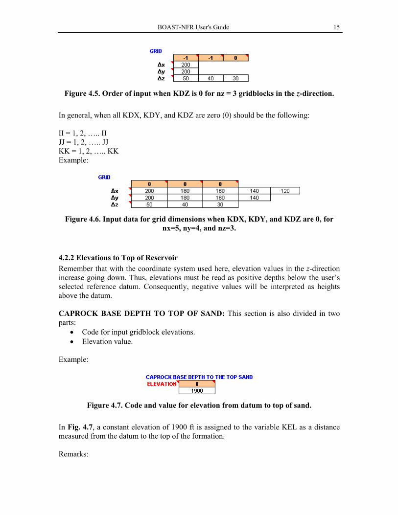
Figure 4.5. Order of input when KDZ is 0 for nz = 3 gridblocks in the z-direction.
In general, when all KDX, KDY, and KDZ are zero (0) should be the following: II = 1, 2, ….. II JJ = 1, 2, ….. JJ KK = 1, 2, ….. KK Example:
Figure 4.6. Input data for grid dimensions when KDX, KDY, and KDZ are 0, for
nx=5, ny=4, and nz=3.
4.2.2 Elevations to Top of Reservoir Remember that with the coordinate system used here, elevation values in the z-direction increase going down. Thus, elevations must be read as positive depths below the user’s selected reference datum. Consequently, negative values will be interpreted as heights above the datum. CAPROCK BASE DEPTH TO TOP OF SAND: This section is also divided in two parts:
• Code for input gridblock elevations. • Elevation value.
Example:
Figure 4.7. Code and value for elevation from datum to top of sand.
In Fig. 4.7, a constant elevation of 1900 ft is assigned to the variable KEL as a distance measured from the datum to the top of the formation. Remarks:

BOAST-NFR User's Guide 16
(1) If KEL = 0, a single constant value is read for the elevation at the top of all gridblocks in Layer 1. (i.e., horizontal plane).
(2) If KEL = 1, a separate elevation value must be read for each gridblock in
Layer 1. II x JJ values must be read in the following order:
J = 1, I = 1,2, . . . .II J = 2, I = 1,2, . . . .II ............................. J = JJ, I = 1,2,. . . . II
Example:
Figure 4.8. Input data order for elevation in a 5x4x3 grid system. Distances
measured below the datum defined by the user. (3) Elevations to the top of the gridblocks in layers below Layer 1 will be
calculated by adding the layer thickness to the preceding layer elevation; i.e.,
TOP(I,J,K=1) = TOP(I,J,K) + DZ(I,J,K)
4.2.3 Porosity and Permeability Distributions Porosity and permeability distributions are entered for matrix and fracture systems in separate sections: Matrix System: There are two parts for this input entry:
• Codes controlling input entries. • Values for porosity, and permeability in the x-, y-, and z-directions.
KPH = Code for controlling porosity input data (See Table 4.2).
KKX = Code for controlling x-direction permeability (See Table 4.2). KKY = Code for controlling y-direction permeability (See Table 4.2). KKZ = Code for controlling z-direction permeability (See Table 4.2). Example:

BOAST-NFR User's Guide 17
Figure 4.9. Porosity and permeability distributions for the matrix system.
In Fig. 4.9, porosity and permeabilities are uniform over the grid. Only one porosity value and one permeability value for each x-, y- and z-direction are to be read. Note: (a) Porosity is read as a fraction (not as a percentage).
(b) See Table 4.2 for the number of values. When KPH = + 1, the order of input must be as indicated below with layer order.
K = 1,2, . . . KK J = 1, I = 1,2, . . . . II J = 2, I = 1,2, . . . . II
.............................. J = JJ, I = 1,2,. . . . II
Note: (a) Permeabilities read in millidarcies (md); KX is a real variable. (b) See Table 4.2 for the number of values. When KKX = + 1, the order of input
must be as indicated below with layer order K = 1, 2, …. KK: K = 1,2, . . . KK J = 1, I = 1,2, . . . . II J = 2, I = 1,2, . . . . II
…............................... J = JJ, I = 1,2,. . . . II Note: See Table 4.2 for the number of values. When KKY = + 1, the order of input must be as indicated below with layer order K = 1, 2, …. KK:
K = 1,2, . . . KK J = 1, I = 1,2, . . . . II J = 2, I = 1,2, . . . . II
…............................... J = JJ, I = 1,2,. . . . II Note: See Table 4.2 for the number of values. When KKZ = + 1, the order of input must be as indicated below with layer order K = 1, 2, …. KK:
K = 1,2, . . . KK J = 1, I = 1,2, . . . . II J = 2, I = 1,2, . . . . II
…...............................

BOAST-NFR User's Guide 18
J = JJ, I = 1,2,. . . . II Fracture System: Two parts for this input entry:
• Codes controlling input entries • Values for porosity, and permeability in the x-, y-, and z-directions
KFPH = Code for controlling porosity input data (See Table 4.3) KWF = Code for controlling fracture width input data (See Table 4.3) KLF = Code for controlling fracture spacing input data (See Table 4.3) KKT = Code for controlling the symmetric fracture permeability tensor, kxx [md] (See Table 4.3)

BOAST-NFR User's Guide 19
Table 4.2. Options for gridblock properties for the matrix system.
Code
Value
Porosity and permeability specifications
-1 Porosity is uniform over the grid; input only one φm value
0 Porosity varies by layer; input KK values of φm
KPH
1 Porosity varies over the entire grid; input II x JJ x KK values
of φm
-1 X-direction permeability is uniform over the grid; input only
one kx value
0 X-direction permeability varies by layer; input KK values of kx
KKX
1 X-direction permeability over the entire grid; input II x JJ x KK
values of kx
-1 Y-direction permeability is uniform over the grid; input only
one ky value
0 Y-direction permeability varies by layer; input KK values of ky
KKY
1 Y-direction permeability over the entire grid; input II x JJ x KK
values of ky
-1 Z-direction permeability is uniform over the grid; input only
one kz value
0 Z-direction permeability varies by layer; input KK values of kz
KKZ
1 Z-direction permeability over the entire grid; input II x JJ x KK
values of kz

BOAST-NFR User's Guide 20
Table 4.3. Options for gridblock properties for the fracture system.
Code
Value
Porosity and permeability specifications
-1 Fracture porosity is uniform over the grid; input only one φf value
0 Fracture porosity varies by layer; input KK values of φf
KFPH
1 Fracture porosity varies over the entire grid; input II x JJ x KK
values of φf
-1 Fracture width is uniform over the grid; input only one wf value
0 Fracture width varies by layer; input KK values of wf
KWF
1 Fracture width over the entire grid; input II x JJ x KK values of
wf
-1 Fracture spacing is uniform over the grid; input only one L
value
0 Fracture spacing varies by layer; input KK values of L
KLF
1 Fracture spacing over the entire grid; input II x JJ x KK values
of L
-1 Permeability tensor is uniform over the grid; input only one full
permeability tensor
0
Permeability tensor varies by layer; input KK full permeability tensors
KKT
1 Permeability tensor over the entire grid; input II x JJ x KK full
permeability tensors

BOAST-NFR User's Guide 21
The permeability tensor has the following components
Figure 4.10. Full permeability tensor.
Example:
Figure 4.11. Porosity and permeability distributions for the fracture system. Fracture permeability is modeled with a diagonal permeability tensor in this
example.
4.2.4 Inter-Porosity Flow Model This section allows choosing a constant shape factors for computing interporosity flow in 1-dimensional, 2-dimensional or 3-dimensional matrix geometry as well as a 1-dimensional time dependent shape factor. Therefore, 4 options are available as expressed in Table 4.4:
Table 4.4. Options for shape factors.

BOAST-NFR User's Guide 22
4.2.5 Faults This section allows to input sealing faults, which are assumed vertical planes that go across the reservoir from the top to the bottom. Figure 4.12 is an example where there are no sealing faults in the model.
Figure 4.12. Default values used where there are no faults in the reservoir.
Fault location is determined by the gridblock number in the x- and y-direction, and the relative position of the fault in the block. For instance, gridblock labeled (2,4,1) contains a sealing fault as illustrated in Fig. 4.13. This fault is represented by two segments given in Fig. 4.14 both located at (2,4). Vertical segment is labeled E because the fault is at the east of the gridblock center and the horizontal segment is labeled N because the fault is located at the north of the gridblock center.
Fault
Block (2,4,1)
Fault segments
N
E
Block (2,4,1)
Figure 4.13. Location of a sealing fault in gridblock (2,4,1). Two segments are used to represent the fault. These segments are no-flow boundaries (zero horizontal
transmissibility)
Figure 4.14. Representation of the fault shown in Fig. 4.13.
4.2.6 Relative Permeabilities and Capillary Pressures These data are entered separately for the matrix and fracture systems. All the relative permeability to oil, water, and gas are presented as function of fluid saturations. For

BOAST-NFR User's Guide 23
example, as oil relative permeability is a function of oil saturation; water relative permeability is a function of water saturation; and gas relative permeability is a function of gas saturation. The same is for capillary pressures. Figure 4.15 is an example of input parameters.
Figure 4.15. Relative permeability and capillary functions for the matrix system.
Note: (1) SAT value at the end of the table must be 1. (2) Read each saturation as a fraction in ascending order.
(3) Read as many lines as there are table entries. In Fig.4.15, fourteen entries were first specified at the top of table.
(4) KRO, KRW etc. are real variables.
Saturation greater than or equal to 1.10 specifies the end of the relative permeability/capillary pressure data.
SAT = Phase saturation. KRO = Oil phase relative permeability, fraction. KRW = Water phase relative permeability, fraction. KRG = Gas phase relative permeability, fraction. PCOW = Oil-water capillary pressure, psi. PCGO = Gas-oil capillary pressure, psi.
Remarks: SAT refers to the saturation of each particular phase.
Example: In a data line following SAT = 0.3; KRO would refer to the oil relative permeability in the presence of 30% oil saturation, KRW would refer to the water relative permeability in the presence of 30% water saturation; KRG would refer to the gas relative permeability in the presence of 30% gas saturation; PCOW would refer to the oil-water capillary pressure in the presence of 30% water saturation, and PCGO would refer to the gas-oil capillary pressure in the presence of 30% gas saturation.
The same applies to the fracture system (See Fig. 4.16).

BOAST-NFR User's Guide 24
Figure 4.16. Relative permeability and capillary functions for the fracture system.
4.2.7 Rock-Fluid Properties at the Fracture/Matrix Interface When using the time-dependent flow correction factor for interporosity flow model (see Section 4.2.4), rock-fluid properties at the fracture/matrix interface as shown in Fig. 4.17 need to be specified.
Figure 4.17. Rock-fluid properties at the interface.
In Fig. 4.17, parameters are:
Sor = Residual oil saturation after the imbibition process, fraction. Swc = Connate water saturation, fraction. krw* = End point relative permeability to water or maximum water relative permeability at the interface during imbibition. no = Curvature of oil relative permeability given as the exponent in the Corey function. dPcdSw = Derivative of capillary pressure with respect to water saturation evaluated at the water saturation at the interface. It can be assumed that the water saturation at the interface is 1-Sor.
4.2.8 Rock Compressibilities Both matrix and fracture compressibilities are entered as function of pore pressure. Example:
Figure 4.18. Rock compressibility for matrix and fracture systems as function of
pore pressure.

BOAST-NFR User's Guide 25
Where, The value next to the header “ROCK” represents the number of points per set (2 in example given in Fig. 4.18). P = pressure, psia Cm = matrix compressibility, psi-1 Cf = fracture compressibility, psi-1
4.2.9 PVT Data The following data is entered in this section:
PBO = Initial reservoir oil bubble-point pressure, psia VSLOPE = Slope of the oil viscosity versus pressure curve for pressure above PBO (i.e., for under-saturated oil). This value is in cp/psi BSLOPE = Slope of oil formation volume factor versus pressure curve for pressure above PBO (i.e., for under-saturated oil). This value is in RB/STB/psi. RSLOPE = Slope of the solution gas-oil ratio versus pressure curve for pressure above PBO (i.e., for under-saturated oil). This value is in SCF/STB/psi IREPRS = Code for repressurization algorithm (see Table 4.5).
Table 4.5. Options for repressurization algorithm.
Example:
Figure 4.19. PVT input data.
Notes:
(1) VSLOPE, BSLOPE and RSLOPE are used only for undersaturated oil (2) BSLOPE should be a negative number and is related to undersaturated oil
compressibility, Co by Co = BSLOPE/BO (3) Normally, RSLOPE will be zero (4) If IREPRS = 0, a new bubble-point pressure will be calculated for each gridblock
containing free gas at the end of each timestep.

BOAST-NFR User's Guide 26
4.2.10 Oil PVT Data The following data are entered:
P = Pressure, psia MUO = Oil viscosity, cp BO = Oil formation volume factor, RB/STB RSO = Solution gas-oil ratio, SCF/STB
Example:
Figure 4.20. Oil PVT data. The value next to the header is equal to the number of
pressure values in table (11 in this case). Note:
(1) Oil properties must be entered as saturated data over the entire pressure range. Laboratory saturated oil data will generally have to be extrapolated above the measured bubble-point pressure to cover the maximum pressure range anticipated during the simulation run. The saturated oil data are required because of the bubble-point tracking scheme used by BOAST-NFR.
(2) The saturated oil data above the initial bubble point pressure will only be used if the local reservoir pressure rises above the initial bubble point pressure and free gas is introduced. An example of this would be pressure maintenance by gas injection into the oil zone.
4.2.11 Water PVT Data The following data are entered:
P = Pressure, psia MUW = Water viscosity, cp BW = Water formation volume factor, RB/STB RSW = Solution gas-water ratio, SCF/STB
Example:
BOAST-NFR User's Guide 27
Figure 4.21. Water PVT data. The value next to the header is equal to the number
pressure values (2 in this case).
Note:
(1) The assumption is often made in black oil simulations that the solubility of gas in reservoir brine can be neglected. This model incorporates this water PVT table to handle such situations as gas production from geo-pressured aquifers, or any other case where gas solubility in water is considered to be of significance to the solution of the problem.
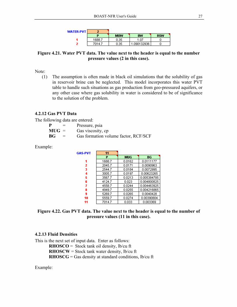
4.2.12 Gas PVT Data The following data are entered:
P = Pressure, psia MUG = Gas viscosity, cp BG = Gas formation volume factor, RCF/SCF
Example:
Figure 4.22. Gas PVT data. The value next to the header is equal to the number of
pressure values (11 in this case).
4.2.13 Fluid Densities This is the next set of input data. Enter as follows:
RHOSCO = Stock tank oil density, lb/cu ft RHOSCW = Stock tank water density, lb/cu ft RHOSCG = Gas density at standard conditions, lb/cu ft
Example:

BOAST-NFR User's Guide 28
Figure 4.23. Oil, water, and gas phase densities in lb/cu ft.
Note:
(1) Stock tank conditions are 14.7 psia and 60º F (2) If no gas exists, set RHOSCG = 0.0
4.2.14 Pressure and Saturation Initialization BOAST-NFR contains two options for pressure and saturation initialization: Option 1: Initial pressure and saturation distributions are calculated based on equilibrium conditions using the elevations and pressure of the gas-oil and water-oil contacts. Option 2: Alternatively, the initial pressure distribution can be read on a block-by-block basis, as in the case of a non-equilibrium situation.
Saturations can either be read as constant values for the entire grid (option 1) or the entire So and Sw distributions are read on a block-by-block basis, and the program calculates the Sg distribution for each block as Sg = 1.0 – So – Sw (option 2).
KPI = Code for controlling pressure initialization (see Table 4.6) KSI = Code for controlling saturation initialization (see Table 4.6)
Table 4.6. Pressure and saturation initialization codes
KPI Description
0 Initial pressure is constant over the entire grid
1 Initial pressure varies in each gridblock
KSI Description
0 Initial fluid saturations are constant over the entire grid
1 Initial fluid saturations vary in each gridblock
For pressure initialization, the following definitions apply:
PWOC = Pressure at the water-oil contact, psia PGOC = Pressure at the gas-oil contact, psia WOC = Depth to the water/oil contact, in feet below datum GOC = Depth to the gas/oil contact, in feet below datum
Example:

BOAST-NFR User's Guide 29
Figure 4.24. Pressure and saturation initialization for matrix system. In the example above (Fig. 4.24), constant input values of pressure and saturations are:
PWOC = 6000 psia PGOC = 5333 psia WOC = 2225 ft below datum GOC = 2000 ft below datum
Note:
(1) PWOC and PGOC are used together with depth to calculate the initial oil phase pressure at each gridblock mid point.
(2) If KPI and KSI = 1, then input the values as indicated below with layer order K = 1,2,……, KK J = 1 I = 1,2,….., II J = 2 I = 1,2,. . . . II ................................... J = JJ I = 1,2, . . . . II
For saturation initialization, the following applies:
SOI = Initial oil saturation. SWI = Initial water saturation.
Example: See Fig. 4.24. In that example,
SOI = 0.8 SWI = 0.2
The initial gas saturation is internally calculated. For the example, the calculated
initial gas saturation would be zero. Note:
(1) Input all saturation values as a fraction. (2) In a non-equilibrium case when KSI = 1, then the order of input must be as
indicated below with layer order K = 1,2,….., KK J = 1 I = 1,2,. . . . , II J = 2 I = 1,2, . . . . II ............................... J = JJ I = 1,2, . . . . II
The same definitions given above apply to the pressure and saturation initialization in
the fracture system.

BOAST-NFR User's Guide 30
Example:
Figure 4.25. Pressure and saturation initialization for the fracture system.
4.2.15 Run Control Parameters This section requires the following data:
NMAX = Maximum number of timesteps allowed before run is terminated. FACT1 = Factor for increasing timestep size under automatic timestep control (set FACT1 = 1.0 for fixed timestep size). FACT2 = Factor for decreasing timestep size under automatic timestep control (set FACT2 = 1.0 for fixed timestep size). TMAX = Maximum simulation run time, days (run will be terminated when time exceeds TMAX). WORMAX = Limiting maximum field water-oil ratio, in STB/STB; simulation will be terminated if total producing WOR exceeds WORMAX. GORMAX = Limiting maximum field gas-oil ratio, in SCF/STB; simulation will be terminated if total producing GOR exceeds GORMAX. PAMIN = Limiting minimum bottomhole flowing pressure, psia; simulation will be terminated if bottomhole pressure in a well falls below PAMIN. PAMAX =Limiting maximum bottomhole flowing pressure, psia; simulation will be terminated if bottomhole pressure in a well exceeds PAMAX.
Example:
Figure 4.26. Run control parameters.
The above example specifies that the simulation will be terminated if:
(a) simulation timesteps exceed 1000 or (b) simulation run time exceeds 1 year (365 days) or (c) total producing, water-oil ratio exceeds 20 STB/STB or

BOAST-NFR User's Guide 31
(d) total producing, gas-oil ratio exceeds 500,000 SCF/STB or (e) bottomhole pressure in a well falls below 14.7 psia or (f) bottomhole pressure in a well exceeds 10,000 psia.
Note:
(1) Timestep size cannot be less than DTMIN nor greater than DTMAX as specified in the recurrent data section
(2) For fixed timestep size, specify FACT1 = 1.0 and FACT2 = 1.0 and/or specify DTMIN = DTMAX = DT in the recurrent data section
(3) For automatic timestep control, set FACT1 > 1.0 and FACT2 < 1.0; suggested values are FACT1 = 1.2 and FACT2 = 0.5
(4) Automatic timestep control means the following: • If at the beginning of a timestep, the maximum gridblock pressure and
saturation changes from the previous step are less than DPMAX and DSMAX, respectively (DPMAX and DSMAX are defined in Section 4.19), the size of the current timestep will be increased by FACT1
• If at the beginning of a timestep, the maximum gridblock pressure or saturation change from the previous step is greater than DPMAX or DSMAX, respectively, the size of the current timestep will be deceased by FACT2
• If at the end of one iteration (after new pressures and saturations are calculated), the maximum pressure change exceeds DPMAX or the maximum saturation change exceeds DSMAX, and FACT2 < 1.0, the size of the current timestep will be decreased by FACT2 and the iteration will be repeated.
4.2.16 Solution Method Control Parameters This section specifies various parameters for controlling the LSOR solution method.
MITR = Maximum number of LSOR iterations for convergence; a typical value is 300. OMEGA = Initial LSOR acceleration parameter. The initial value for OMEGA must be in the range 1.0 < OMEGA < 2.0. A typical initial value for OMEGA is 1.70. The model will attempt to optimize OMEGA as the solution proceeds if TOL is greater than zero. TOL = Maximum acceptable pressure change for LSOR convergence; a typical value is 0.1 psi. TOL1 = Parameter for determining when to change (i.e. optimize) OMEGA; a typical value is 0.0005. If TOL1 = 0.0 the initial value of OMEGA will be used for the entire simulation. DSMAX = Maximum saturation change (fraction) permitted over a timestep. The timestep size will be reduced by FACT2 if FACT2 < 1.0, and the saturation change of any phase in any gridblock exceeds DSMAX and the current step-size is greater than DTMIN. If the resulting step-size is less than DTMIN, the

BOAST-NFR User's Guide 32
timestep will be repeated with the step-size DTMIN. A typical value of DSMAX is 0.05. DPMAX = Maximum pressure change (psi) permitted over a timestep. The timestep size will be reduced by FACT2 if FACT2 < 1.0 and the pressure change in any gridblock exceeds DPMAX and the current step-size is greater than DTMIN. If the resulting step-size is less than DTMIN, the timestep will be repeated with step-size DTMIN. A typical value of DPMAX is 50 psi.
Example:
Figure 4.27. Parameters controlling the LSOR solution method.
BOAST-NFR User's Guide 33
5. Recurrent Data
5.1 Introduction During the course of a simulation run, it is generally desirable to be able to (1) add or delete injection/production wells, (2) control injection/production rates or bottomhole pressures at all existing wells, and (3) specify the types and frequency of output information. These types of controls and output specifications are accomplished in this model via "recurrent data" records. That is, as the simulation proceeds, well specification and print control information is input at preselected times.
Recurrent data record pairs are input which control printed output and timestep size for a specified time period. The first parameter (IWLCNG) on the first recurrent data record specifies whether or not to read well information. If IWLCNG = 0, well information is not read. If IWLCNG = 1, well information is read immediately following the recurrent data record pair. In any case, the simulator advances through timesteps until the specified elapsed time (ICHANG times DT) has occurred. During this period, all print codes and the latest well information applies. At the end of this period, a new set of recurrent data records are read and the process is repeated.
Modification of the recurrent data records occasionally needs to be done under the restart option. This is because all of the recurrent data is written to the restart file. If a waterflood is begun under restart conditions after any given period of primary production during a phase 1 run, and then restarted and continued in a phase 2 period, the recurrent data records for the primary recovery must first be removed.
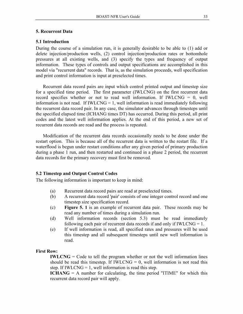
5.2 Timestep and Output Control Codes The following information is important to keep in mind:
(a) Recurrent data record pairs are read at preselected times. (b) A recurrent data record 'pair' consists of one integer control record and one
timestep size specification record. (c) Figure 5. 1 is an example of recurrent data pair. These records may be
read any number of times during a simulation run. (d) Well information records (section 5.3) must be read immediately
following each pair of recurrent data records if and only if IWLCNG = 1. (e) If well information is read, all specified rates and pressures will be used
this timestep and all subsequent timesteps until new well information is read.
First Row:
IWLCNG = Code to tell the program whether or not the well information lines should be read this timestep. If IWLCNG = 0, well information is not read this step. If IWLCNG = 1, well information is read this step. ICHANG = A number for calculating, the time period "ITIME" for which this recurrent data record pair will apply.

BOAST-NFR User's Guide 34
IWLREP = Output code for printing well report. ISUMRY = Output code for printing summary report. IPMAP = Output code for printing pressure distribution. ISOMAP = Output code for printing oil saturation distribution. ISWMAP = Output code for printing water saturation distribution. ISGMAP = Output code for printing gas saturation distribution. IOPRMAP = Output code for printing inter-porosity oil rate distribution. IWPRMAP = Output code for printing inter-porosity water rate distribution. IPBMAP = Output code for printing bubble-point pressures (normally set IPBMAP = 0).
Second Row:
DT = Initial timestep size (days) for this period. DTMIN = Minimum timestep size (days) for this period. DTMAX = Maximum timestep size (days) for this period.
Example:
Figure 5.1. Recurrent data pair for timestep and output control.
The above example specifies that:
(a) Well information is read at this step. (b) 1 is to be used as the number for calculating the time period for which this
recurrent data will apply (i.e. ICHANG = 1) (c) Well report and summary reports are to be printed at this step; and (d) None of the other maps are to be printed at this step. (e) DT = 0.0001 days (f) DTMIN = 0.00001 days (g) DTMAX = 0.001 days.
Note:
(1) If IWLCNG = 1, well information lines must be read. The new well information will apply during the next timestep.
(2) If 'ETI' is the time at the beginning of the current step, then this recurrent data record pair will apply from ETI until FTMAX.
Where, ITIMEETIFTMAX += ,
DT*ICHANGITIME = , DT is the initial timestep size.
(3) The actual number of timesteps for which ICHANG is used will likely be
different from ICHANG if automatic timestep control is “ON.” Whenever the calculated simulation time exceeds 'FTMAX,' the current step-size is reduced

BOAST-NFR User's Guide 35
to give an elapsed time of exactly FTMAX. Whenever FTMAX is reached, another recurrent data record pair is read.
(4) If the output code value = 0, the information will not be printed. (5) If the output code value = 1, the information will be printed for each timestep
during this period from ETI days to FTMAX days. (6) If DT = DTMIN = DTMAX, the automatic timestep control is overridden. (7) Common (suggested) values for DTMIN and DTMAX are 0.0001 and 0.01
days, respectively. (8) If automatic timestep control is not specified (i.e., FACT1 = FACT2 = 1.0) it
is convenient to specify DTMIN = 0.0 and DTMAX = DT. (9) Recurrent data records should be input until the cumulative time as given by
the summation of ICHANG times DT for each pair exceeds the maximum desired simulation time (TMAX).
5.3 Well Information Records This section is used to describe well activities. The first row specifies the total number of vertical/horizontal/slanted wells for which well information is to be read. Where,
NVQN = Number of vertical wells NVQNH = Number of horizontal wells NVQNS = Number of slanted wells
Example:
Figure 5.2. Well information records showing one vertical producing well.
5.3.1 Vertical Well Information Enter the following information in the same order in the second row: I, J, PERFI, NLAYER, KIP, QO, QW, QG, QT Where,
I = X-coordinate of gridblock containing this well (i.e. 10) J = Y-coordinate of gridblock containing this well (i.e. 1) PERFI = Layer number of the uppermost layer completed (i.e. 1). NLAYER = Total number of consecutive completion layers, starting with and including PERFI (i.e. 3). KIP = Code for specifying both well type and whether the well's production (injection) performance is determined by specifying rates or specifying flowing bottomhole pressure and also whether an explicit or implicit pressure calculation is to be made. For most cases, the implicit pressure calculation is recommended. See Table 5.1 for the code details. For more information on KIP see the notes at the end of this section (i.e. 1).

BOAST-NFR User's Guide 36
QO = Oil rate, STB/D (nonzero only if KIP = 1 and QT = 0.0) (i.e. 0) QW = Water rate, STB/D (nonzero only if KIP = 2) (i.e. 0) QG = Gas rate, MCF/D (nonzero only if KIP = 3) (i.e. 0) QT = Total fluid rate (nonzero only if KIP = 1 and QO = 0.0) (i.e. 1000).
The example shown in Fig. 5.2 specifies that the well “VER Prod” is located in the gridblock (10,1,1); completed in 3 layers and produces a total fluid rate of 1000 STB/D. Note:
(1) Wells may be added or re-completed at any time during the simulation. However, once a well has been specified, it must be included in each timestep that well information is read, even if the well is currently shut-in.
(2) Table 5.1 summarizes all well control options. (3) NLAYER must include all layers from PERFI to the lower most layer
completed. For example, in a 5-layer model, if a well is completed in layers 2, 3, and 5, set PERFI = 2 and NLAYER = 4. Note that in this, layer 4 must be included in NLAYER even though layer 4 is not perforated. Layer 4 may be shut in by specifying the PID value for layer 4 as zero.
(4) Exactly NLAYER lines must be read for each WELLID (even if the well is rate controlled). Each of these lines specifies a layer flow index (PID) and flowing, bottomhole pressure (FBHP) for one completion layer; thus, NLAYER of these lines must be read. The first line read applies to the uppermost completion layer (PERFI); additional lines apply to succeeding layers. If rates are specified for this well (KIP = +1, +2, or +3), PWF will not be used and should be read as zero; however, PID will be used to calculate a FBHP for the well. This FBHP will be printed out on the well report, but it will not be used in any way to control the well performance.
(5) Negative rates indicate fluid injection; positive values indicate fluid production.
(6) The total fluid rate given by QT is the oil plus water plus gas production for the well or the total reservoir voidage at stock tank conditions.
(7) Only one of the four values (QO, QW, QG, or QT) may be nonzero. If KIP < 0, all four values should be zero.
(8) If KIP = 2, -2 or -12, only water will be produced or injected; if KIP = 3, -3, or -13, only gas will be produced or injected; solution gas is not considered; therefore, these options are only recommended for water or gas injection wells. If KIP = 1, - 1, or - 11, oil, water, and gas will be produced in proportion to fluid mobilities and pressure constraints.
(9) For most applications, implicit pressure calculations are recommended. (10) If KIP > 0, the specified rate will be allocated to layers based on total layer
mobilities; e.g.; if QW is specified and there are two layers QW1 = QW * TM1/(TM1 + TM2) and QW2 = QW * TM2/(TM1 + TM2), where TM1 = total mobility for layer 1 and TM2 total mobility for layer 2.

BOAST-NFR User's Guide 37
Subsequent Rows: Use these rows to enter flowing, bottomhole pressure and productivity index information for vertical wells.
PID = Layer productivity index PWF = Layer flowing bottomhole pressure, psia
Note:
(1) If rates are specified (i.e. KIP > 0) for this well, PWF is not required and should be specified zero.
(2) If rates are specified (i.e. KIP > 0) for this well and PID is specified nonzero, the specified rate and PID will be used to calculate and print a flowing bottomhole pressure. However, the calculated pressure will not be used to control well performance.
(3) Once a well has been specified in any layer, that well and that layer must be specified each time well information lines are read.
(4) To shut in a layer, set the layer PID = 0.0; to shut in a well, simply set all its layer PID's = 0.0.
(5) The layer PID may be calculated from the following equation:
+
=Sr
rln
0.00708khPID
w
e
where, re = equivalent gridblock radius, ft rw = wellbore radius, ft h = Z-dimension (layer thickness) of the block, ft k = mean X-Y permeability in md S = layer skin factor

BOAST-NFR User's Guide 38
Table 5.1. Options for controlling well performance.

BOAST-NFR User's Guide 39
The radius re may be calculated from Peaceman's formula:
+
+
=41
41
21
221
221
28.0r
y
x
x
y
y
x
x
y
e
kk
kk
dykk
dxkk
where, Kx = permeability in x-direction Ky = permeability in y-direction dx = X-direction gridblock dimension, ft dy = Y-direction gridblock dimension, ft
(6) Formation damage or stimulation at any point in time can be handled on a layer-by-layer basis by changing the layer PID.
(7) Line 5 must be read NLAYER times
The above example specifies that well number 2 is an injection well (INJ1), is located
in the gridblock (1,1,1), completed in one layer; the well is a water injection well (KIP = 2) and the injection rate is 900 STB/D. The layer productivity index for this well is 10.0 and the flowing bottomhole pressure 7500 psia will not be used in calculations.
5.3.2 Horizontal Well Information Enter the following information right next to the well name: LAYER, KIP, QVO, QVW, QVG, QVT, COND
LAYER = Total number of consecutive well bore blocks KIP, QVO, QVW, QVG, QVT = same definitions as KIP, QO, QW, QG and QT described in vertical producer, respectively COND = code for specifying, type of wellbore conductivity in well rate calculations
When COND = 1, infinite conductivity is used When COND = 2, "uniform flux" is chosen
Example:

BOAST-NFR User's Guide 40
Figure 5.3. Well information records showing a horizontal well.
IQH1 = X - coordinate of gridblock containing, this well. IQH2 = Y - coordinate of gridblock containing, this well. IQH3 = Z - coordinate of gridblock containing, this well. PIDMTX = gridblock productivity index of matrix system, Peaceman's formula is suggested except that kx (or ky) is replaced by kz when the horizontal wellbore is parallel to the y (or x) axis. PWF = gridblock flowing bottomhole pressure.
5.3.3 Slanted Well Information Enter the following information right next to the well name: IFLAG, KIP, QVO, QVW, QVG, QVT, COND
IFLAG = Code for specifying ways to define the geometric location of slanted well in reservoir gridblocks. Two options are defined below. KIP, QVO, QVW, QVG, QVT, COND = Same codes as in horizontal wells
IFLAG: (a) If IFLAG is 1, then enter the following data below the input codes row: IS, JS,
KS, WELENGTH, THETA, ALPHA, IS1, IS2, IS3. Where,
IS = X - coordinate of starting gridblock for defining this well. JS = Y - coordinate of starting gridblock for defining this well. KS = Z - coordinate of starting gridblock for defining this well. WELENGTH = Total wellbore length in feet of this well. THETA = Slant angle in degree which wellbore deviated from the downward direction as shown in Fig. 5.4, i.e.; vertical well downward has a THETA of 0 (0 < THETA < 180). ALPHA = Area angle in degree which wellbore departed from the increasing direction of x-axis from the plan view as shown in Fig. 5.5 (0 < ALPHA < 360) IS1 = X-coordinate of starting gridblock of the producing wellbore, i.e.; wellbore gridblock of x-coordinate from IS to IS1-1 are not productive.

BOAST-NFR User's Guide 41
Figure 5.4. Side view showing angle theta.
Figure 5.5. Top view of grid showing angle alpha.
JS1 = Y-coordinate of starting, gridblock of the producing wellbore. Wellbore gridblocks of y-coordinate from JS to JS1-1 are not productive. KS1 = Z-coordinate of starting, gridblock of the producing wellbore. Wellbore gridblocks of z-coordinate from KS to KS1-1 are not productive.
Example:

BOAST-NFR User's Guide 42
Figure 5.6. Well information records showing a slanted well with IFLAG = 1.
Figure 5.6 above indicates a slanted wellbore starting from (1, 1, 1) is 1000 ft long
and 60 degrees from the downward direction and 315 degrees from the x-axis. This slanted well has productive wellbore block starting from (1, 1, 1). (b) If IFLAG is 2, then enter the following data below the input codes row: IS, JS, KS, IE, JE, KE, IS1, JS1, KS1. Where,
IE = X-coordinate of ending gridblock of this well. JE = Y-coordinate of ending gridblock of this well. KE = Z-coordinate of ending gridblock of this well. IS, JS, KS, IS1, JS1, KS1 are defined same as those in option (a) when IFLAG=1.
Example:
Figure 5.7. Well information records showing a slanted well with IFLAG = 2.
Figure 5.7 above indicates a slanted wellbore starting from (3, 1, 1) and ending at (8,
1, 5). The productive wellbore block starts from (5, 1, 2) as shown in Fig. 5.8.

BOAST-NFR User's Guide 43
Figure 5.8. Side view of a slanted wellbore showing position in x-z plane.
Wellbore Characteristics: Enter the following information in the row below the parameters defining the position of the well: RW, S, PWF, JFLAG Where, RW = wellbore radius, ft S = wellbore skin factor PWF = gridblock flowing bottom hole pressure, psi. JFLAG = code for specifying ways to initialize wellbore pressure
If JFLAG = 1, PWF will be assigned to all wellbore blocks If JFLAG = 2, wellbore pressure will be calculated for each wellbore block based on hydraulic gradient and PWF as wellbore pressure of the starting wellbore block.
Figures 5.6 and 5.7 specify the wellbore has a radius of 0.3 ft with 0 skin and a
flowing pressure of 100 psi which will be assigned to all wellbore blocks.

BOAST-NFR User's Guide 44
6. Interpretation of Model Output BOAST-NFR program comes with three spreadsheets that are used to write the output data: Output Data, Summary Report and Restart Data spreadsheets. If for some reason one of these sheets is deleted, they need to be created with the names given above for the proper execution of the program. Output Data and Summary Report are always needed while the Restart Data spreadsheet is used only when the Restart Option is activated (see Section 4.2.1).
6.1 Output Data Spreadsheet Four types of reports are written in the Output Data spreadsheet: Material balance report, well report, summary report, and variable distribution arrays.
6.1.1 Material Balance Report Once the program starts running after clicking the icon RUN in Input Data spreadsheet, a material balance for fluids in-place is computed and written in the Output Data spreadsheet. This report is organized such that initial fluid in-place at standard conditions is presented for every layer and for the whole reservoir. For instance, Fig. 6.1 shows a material balance report for a reservoir simulated with one layer.
Figure 6.1. Material balance report written during the first iteration.
In this figure: OOIP = Original oil in-place given in 106 STB. OWIP = Original water in-place given in 106 STB. S_OGIP = Original gas in-place dissolved in oil and water phases given in 109 SCF. F_OGIP = Original gas in-place present as a free phase given in 109 SCF.
6.1.2 Well Report A well report may be specified at any time during the simulation run. Each time a well report is specified, production and injection rates and cumulative volumes for each layer of each well are tabulated and summarized. The following information is provided in this report for each well:

BOAST-NFR User's Guide 45
• Well location (I,J,K), • Calculated bottomhole pressure, psia, • Specified bottomhole pressure, psia, • Productivity index, • Oil production rate, STB/D, • Gas production/injection rate, MSCF/D, • Water production/injection rate, STB/D, • GOR, SCF/STB, • WOR, STB/STB, • Cumulative volumes of production and/or injection (Np, Gp, Wp), • Medium that mainly produces at the well. If well is completed in a gridblock where a
non-zero fracture porosity was specified, fracture is written as the producing medium; otherwise matrix is written.
6.1.3 Summary Report in the Output Data Spreadsheet The summary report is the single most useful report and can also be obtained at any desired time. The summary report contains a concise summary of field injection and production performance information including: • Average reservoir pressure, • Total reservoir oil, water, and gas production rates and cumulative production, • Total reservoir water, and gas injection rates and cumulative injection, • Total reservoir current and cumulative water-oil, and gas-oil ratios, • Timestep and material balances for oil, water, and gas.
The summary report serves two major purposes by permitting, the user to (1) quickly review total reservoir performance and (2) determine if the model is functioning properly. As a general rule, timestep material balance errors should normally be less than 0.1%
Material balances that are excessive do not necessarily mean that the model cannot handle the problem at hand. However, it does mean that adjustments are needed to some of the input parameters. Normally, the first adjustment is reduction of timestep size. If this modification does not completely solve the problem, reduce injection and/or production rates to determine if well controls are excessive based on existing flow capacity and reservoir pressure. By making full use of automatic timestep control and being careful not to over-pressure or overproduce the reservoir, most naturally fracture reservoir engineering problems can be successfully simulated with BOAST-NFR.
6.1.4 Variable Distribution Arrays The user may output pressure, saturation, interporosity rates and bubble-point pressure arrays for both the matrix and the fracture media at any timestep desired. For large two-dimensional or three-dimensional problems, an enormous output file can result if all these arrays are frequently printed. Therefore, these distributions should only be printed when

BOAST-NFR User's Guide 46
absolutely needed. Normally, the bubble-point pressure array need not ever be printed out. This array provides mainly diagnostic information.
The pressure and saturation arrays should always be checked carefully at discrete times during the simulation to assure that overall pressure and saturation trends are as they should be. Also, if a material balance problem exists, these maps may help to isolate the problem.
6.2 Summary Report Spreadsheet As a simulation run progresses, timestep number, total simulation time, average reservoir pressure, oil production rate, cumulative oil production, gas production rate, cumulative gas production, GOR, water production rate, cumulative water production, WOR, Water cut, total interporosity rates, number of iteration for pressure convergence in LSOR are printed for the field being simulated.
Data values are printed according to the time interval specified in NDT (see Section 4.2.1). Since a macro is used to print these data, it can be modified to write any variable of interest using the Visual Basic Editor in MS EXCEL. An example of this spreadsheet is given in Fig. 6.2.
Figure 6.2. Summary Report spreadsheet showing output data for the field every
NDT = 100 timesteps.

BOAST-NFR User's Guide 47
6.3 Restart Data Spreadsheet If the creation of restart data at the end of the simulation run is specified as indicated in Section 4.2.1, input data for a restart simulation run is automatically prepared in the Restart Data spreadsheet at the end of a normal simulation run. Porosity, permeability, gridblock pressures and saturations are written along with all the information required to continue with simulation. For this new data set, ITIME is time at which the normal simulation time ended; and therefore, it is the initial time for the restart run (see Fig. 6.3). To run a restart simulation, use Copy and Paste in the tool bar under Edit to locate data in the Input Data spreadsheet. Be careful while performing this action since you may copy part of the information or you may delete the icon RUN, needed to start the new simulation.
Figure 6.3. Restart Data spreadsheet written at the end of a simulation run.

BOAST-NFR User's Guide 48
7. Example Input and Output Data
7.1 Introduction This section provides one example problem that illustrates the capability of the model to simulate a waterflooding problem in a naturally fractured reservoir. The reservoir and PVT data used for the example problems are not intended to represent any specific reservoir or fluid system. The input data should be considered as "sample data" and their sole purpose is to illustrate the capabilities of the simulator. Users can consider these input data as a guide for building their own input data.
7.2 Problem Description A brief description of the example problem is given below. The input file, summary report and partial output file for the example are also provided in the following.
Input data presented in the following section are taken from the sixth SPE
comparative project for dual-porosity simulators.2 Fluid PVT data and some of the fluid-rock properties for that project were originally presented by Thomas at al.3
The naturally fractured reservoir is simulated as a single-layer formation using a
15×1×1 parallel Cartesian grid whose dimensions are shown in Table 7.1. The reservoir is composed of a matrix system with φm = 29% and kx=ky=kz = 1 md. It is assumed that the fracture network consists of a single set of parallel fractures with φf = 1%, diagonal permeability tensor with kf = 90 md and a fracture spacing of L = 5 ft. Therefore, the matrix-block shape factor using Lim and Aziz’s approximation4 for one set of parallel fractures is σ = 0.396 ft2.
Table 7.1. Gridblock and reservoir rock basic data Number of gridblocks in the x-direction, nx 40
Number of gridblocks in the y-direction, ny 1
Number of gridblocks in the z-direction, nz 1
Gridblock size in the x-direction, ∆x, ft 50
Gridblock size in the x-direction, ∆y, ft 1000
Gridblock size in the x-direction, ∆z, ft 50
Matrix porosity, φm, fraction 0.29
Matrix permeability, km, md 1.0
Matrix compressibility, cm, psi-1 3.5 × 10⁻⁶
Fracture porosity, φf, fraction 0.01
Fracture permeability, kf, md 90
Fracture compressibility, cf, psi-1 3.5 × 10⁻⁶
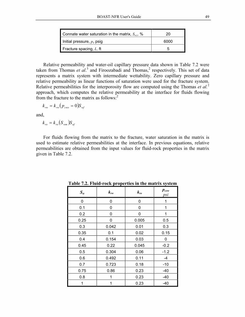
BOAST-NFR User's Guide 49
Connate water saturation in the matrix, Swc, % 20
Initial pressure, pi, psig 6000
Fracture spacing, L, ft 5
Relative permeability and water-oil capillary pressure data shown in Table 7.2 were taken from Thomas et al.3 and Firoozabadi and Thomas,2 respectively. This set of data represents a matrix system with intermediate wettability. Zero capillary pressure and relative permeability as linear functions of saturation were used for the fracture system. Relative permeabilities for the interporosity flow are computed using the Thomas et al.2 approach, which computes the relative permeability at the interface for fluids flowing from the fracture to the matrix as follows:2
( ) wfcworwrw Spkk 0==
and, ( ) ofwmroro SSkk =
For fluids flowing from the matrix to the fracture, water saturation in the matrix is
used to estimate relative permeabilities at the interface. In previous equations, relative permeabilities are obtained from the input values for fluid-rock properties in the matrix given in Table 7.2.
Table 7.2. Fluid-rock properties in the matrix system
Sα krw kro pcow psi
0 0 0 1 0.1 0 0 1 0.2 0 0 1
0.25 0 0.005 0.5 0.3 0.042 0.01 0.3
0.35 0.1 0.02 0.15 0.4 0.154 0.03 0
0.45 0.22 0.045 -0.2 0.5 0.304 0.06 -1.2 0.6 0.492 0.11 -4 0.7 0.723 0.18 -10
0.75 0.86 0.23 -40 0.8 1 0.23 -40 1 1 0.23 -40

BOAST-NFR User's Guide 50
In Table 7.2, Sα represents phase saturation. For instance, fluid-rock properties at Sw=0.3 are krw = 0.042, kro = 0.18, and pcow = 0.3 psi.
PVT data of oil is divided into two sets. One set corresponds to undersaturated
properties relative to a bubble-point pressure pb = 5545 psig (Table 7.3). Saturated values are shown in Table 7.4. In this simulation, pressures remain above the bubble-point pressure; and, therefore mainly undersaturated values are used.
Table 7.3. Undersaturated oil properties Oil density, ρo, lb/ft3 51.14
Oil viscosity at pb, µo, cp 0.21
Slope of µo above pb, dµo/dp, cp/psi 1.72×10⁻⁵
Oil formation volume factor at pb, Bo, RB/STB 1.8540
Slope of Bo above pb, dBo/dp, RB/STB/psi -4.0×10⁻⁵
Table 7.4. Saturated oil properties p
psig µo cp
Bo RB/STB
Rso SCF/STB
1674 0.529 1.3001 367 2031 0.487 1.3359 447 2530 0.436 1.3891 564 2991 0.397 1.4425 679 3553 0.351 1.5141 832 4110 0.31 1.5938 1000 4544 0.278 1.663 1143 4935 0.248 1.7315 1285 5255 0.229 1.7953 1413 5545 0.21 1.854 1530 7000 0.109 2.1978 2259
PVT data of water are basically µw = 0.35 cp, Bw = 1.07 RB/STB, cw = 3.5×10⁻⁶ psi-1 and ρw = 65 lbm/ft3.

BOAST-NFR User's Guide 51
A simulation run was performed by using a producer located at gridblock indexed (1,1,1) and an injector at (15,1,1). Fluid withdrawal was constrained by total liquid production of 800 STB/D while water injection was initially controlled by a constant rate of 1568 STB/D but constrained by a maximum bottomhole pressure of 6100 psig. Results from a simulation run time of 10 years are reported in the Output Data and Summary Report spreadsheets.

BOAST-NFR User's Guide 52
7.3 Input Data DATA nx ny nz 15 1 1 NDT RESTART ITIME 100 1 0 GRID -1 -1 -1
∆x 200 ∆y 1500 ∆z 50
CAPROCK BASE DEPTH TO THE TOP SAND ELEVATION 0
2000 MATRIX POROSITY AND PERMEABILITY -1 -1 -1 -1
φm 0.29 kx 1 ky 1 kz 1
FRACTURE POROSITY AND PERMEABILITY -1 -1 -1 -1
φf 0.01 wf 0.05 L 5.00
kxx 90 kyy 90 kzz 90 kxy 0 kxz 0 kyz 0
INTER-POROSITY FLOW MODEL 1
FAULTS 0 X Y N/E
0 0 N/E MATRIX SAT. 14 SAT KRO KRW KRG PCOW PCGO
1 0 0 0 0 1 0 2 0.1 0 0 0.015 1 0 3 0.2 0 0 0.05 1 0 4 0.25 0 0.005 0.0765 0.5 0 5 0.3 0.042 0.01 0.103 0.3 0 6 0.35 0.1 0.02 0.1465 0.15 0 7 0.4 0.154 0.03 0.19 0 0 8 0.45 0.22 0.045 0.25 -0.2 0 9 0.5 0.304 0.06 0.31 -1.2 0
10 0.6 0.492 0.11 0.538 -4 0 11 0.7 0.723 0.18 0.538 -10 0 12 0.75 0.86 0.23 0.538 -40 0 13 0.8 1 0.23 0.538 -40 0 14 1 1 0.23 0.538 -40 0
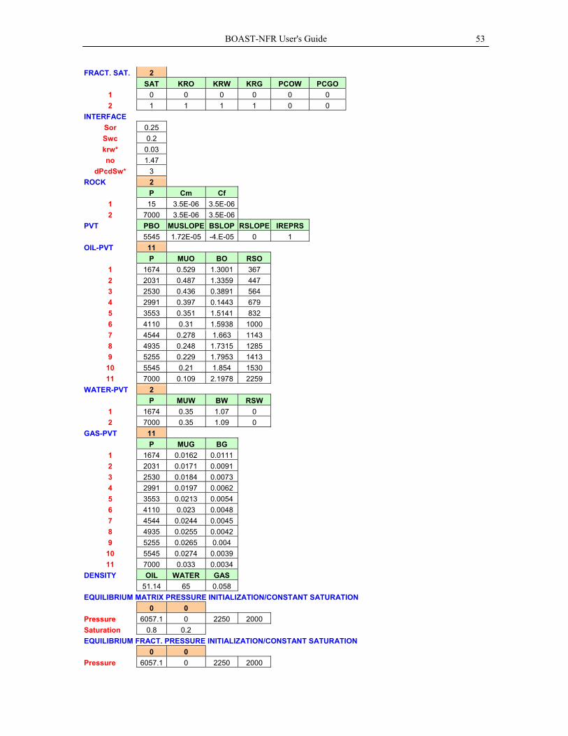
BOAST-NFR User's Guide 53
FRACT. SAT. 2 SAT KRO KRW KRG PCOW PCGO
1 0 0 0 0 0 0 2 1 1 1 1 0 0
INTERFACE Sor 0.25 Swc 0.2 krw* 0.03 no 1.47
dPcdSw* 3 ROCK 2 P Cm Cf
1 15 3.5E-06 3.5E-06 2 7000 3.5E-06 3.5E-06
PVT PBO MUSLOPE BSLOP RSLOPE IREPRS 5545 1.72E-05 -4.E-05 0 1 OIL-PVT 11 P MUO BO RSO
1 1674 0.529 1.3001 367 2 2031 0.487 1.3359 447 3 2530 0.436 0.3891 564 4 2991 0.397 0.1443 679 5 3553 0.351 1.5141 832 6 4110 0.31 1.5938 1000 7 4544 0.278 1.663 8 4935 0.248 1.7315 1285 9 5255 0.229 1.7953 1413
10 5545 0.21 1.854 1530 11 7000 0.109 2.1978 2259
WATER-PVT 2 P MUW BW RSW
1 1674 0.35 1.07 0 2 7000 0.35 1.09 0
GAS-PVT 11 P MUG BG
1 1674 0.0162 0.0111 2 2031 0.0171 0.0091 3 2530 0.0184 0.0073 4 2991 0.0197 0.0062 5 3553 0.0213 0.0054 6 4110 0.023 0.0048 7 4544 0.0244 0.0045 8 4935 0.0255 0.0042 9 5255 0.0265 0.004
10 5545 0.0274 0.0039 11 7000 0.033 0.0034
DENSITY OIL WATER GAS 51.14 65 0.058 EQUILIBRIUM MATRIX PRESSURE INITIALIZATION/CONSTANT SATURATION 0 0 Pressure 6057.1 0 2250 2000 Saturation 0.8 0.2 EQUILIBRIUM FRACT. PRESSURE INITIALIZATION/CONSTANT SATURATION 0 0 Pressure 6057.1 0 2250 2000
1143

BOAST-NFR User's Guide 54
Saturation 1 0 CODES NMAX FACT1 FACT2 TMAX WORMAX GORMAX PMIN PMAX 50000 1.2 0.5 3640 50 100000 200 6100 LSOR MITR OMEGA TOL TOL1 DSMAX DPMAX 1000 1.7 1E-05 0 0.02 50 RECURRENT DATA
TP 1 1 1 1 1 1 1 0 1 1 0 0.0001 0.00001 0.001 0 0 0
RATES 2 0 0 Ver Prod. 1 1 1 1 1 0 0 0 800
1 4.98 0 Ver Inj. 15 1 1 1 2 0 -1568 0 0
1 4.98 0 TP 0 200 0 0 0 0 0 0 0 0 0
0.001 0.0001 0.01 0 0 0 TP 0 200 0 0 0 0 0 0 0 0 0
0.01 0.001 0.1 0 0 0 TP 0 200 0 0 0 0 0 0 0 0 0
0.1 0.1 0.1 0 0 0 TP 0 500 0 0 0 0 0 0 0 0 0
0.1 0.1 0.1 0 0 0 TP 0 500 0 0 0 0 0 0 0 0 0
0.1 0.1 0.1 0 0 0 TP 0 597 0 0 0 0 0 0 0 0 0
0.1 0.1 0.1 0 0 0 TP 0 1 1 1 1 1 1 1 0 0 0
0.1 0.1 0.1 0 0 0 TP 0 1819 0 0 0 0 0 0 0 0 0
0.1 0.1 0.1 0 0 0 TP 0 1 1 1 1 1 1 1 0 0 0
0.1 0.1 0.1 0 0 0 TP 0 1819 0 0 0 0 0 0 0 0 0

BOAST-NFR User's Guide 55
7.4 Output Data
Layer 1OOIP [MMSTB]= 5.2823022OWIP [MMSTB]= 2.1396018S_OGIP [BSCF]= 8.0817232F_OGIP [BSCF]= 0
Total initial fluid volumes in reservoirOOIP [MMSTB]= 5.2823022OWIP [MMSTB]= 2.1396018S_OGIP [BSCF]= 8.0817232F_OGIP [BSCF]= 0
Well Report Time= 0.0001ID Location cBHFP sBHFP PID Qo Qg Qw GOR WOR Np Gp Wp Medium
I J K psia psia STB/D MSCF/D STB/D MSTB MMCF MSTBVer Prod. 1 1 1 5935.74809 0 4.975 800 1223.9698 0 1529.96 0 0.00008 0.000122 0 fractureVer Inj. 15 1 1 -1 6100 4.98 0 0 -2102.1429 0 0 0 0 -0.00021 fracture
Totals 800 1223.9698 -2102.1429 0.00008 0.000122 -0.00021Summary Report
Elapsed time [days]= 0.0001Time-step No = 1Time-step [days]= 0.0001P ave [psi]= 6000.0517
Qo [STB/D]= 800 Np [STB]= 0.08 mbeo [%]= -1.2363E-08Qg [MSCF/D]= 1223.9698 Gp [MSCF]= 0.12239698 mbeg [%]= 2.0177E-09Qw [STB/D]= 0 Wp [STB]= 0 mbew [%]= 9.7687E-15
Qgi [MSCF/D]= 0 Gi [MSCF]= 0Qwi [STB/D]= -2102.143 Wi [STB]= -0.21021429
WOR [STB/STB]= 0GOR [SCF/STB]= 1529.9623
Reservoir pressure distribution in the matrix systemK = 1 6000.0441 6000.0513 6000.051389 6000.05139 6000.0514 6000.05139 6000.05139 6000.0514 6000.05139 6000.05 6000.05 6000.051 6000.051 6000.051 6000.062779
Oil saturation in the matrix systemK = 1 0.8 0.8 0.8 0.8 0.8 0.8 0.8 0.8 0.8 0.8 0.8 0.8 0.8 0.8 0.8
Water saturation in the matrix systemK = 1 0.2 0.2 0.2 0.2 0.2 0.2 0.2 0.2 0.2 0.2 0.2 0.2 0.2 0.2 0.2
Oil flow rate of mass transferK = 1 629.90028 3.3549549 0.01785322 9.5913E-05 5.161E-07 3.0357E-08 3.0357E-08 3.036E-08 3.0357E-08 0 -8E-07 -0.000149 -0.02776 -5.216298 -979.3697919
Water flow rate of mass transferK = 1 0 0 0 0 0 0 0 0 0 0 0 0 0 0 0
Reservoir pressure distribution in the fractured systemK = 1 6000.0063 6000.0511 6000.051387 6000.05139 6000.0514 6000.05139 6000.05139 6000.0514 6000.05139 6000.05 6000.05 6000.051 6000.051 6000.052 6000.121463
Oil saturation in the fractured systemK = 1 1 1 1 1 1 1 1 1 1 1 1 1 1 1 0.999991452
Water saturation in the fractured systemK = 1 0 0 0 0 0 0 0 0 0 0 0 0 0 0 8.54769E-06
Material Balance Report

BOAST-NFR User's Guide 56
Well Report Time= 182ID Location cBHFP sBHFP PID Qo Qg Qw GOR WOR Np Gp Wp Medium
I J K psia psia STB/D MSCF/D STB/D MSTB MMCF MSTBVer Prod. 1 1 1 5810.2416 0 4.975 799.925264 1223.8555 0.07473599 1529.96 9.3E-05 145.5985 222.7602 0.001484 fractureVer Inj. 15 1 1 -1 6100 4.98 0 0 -1339.1437 0 0 0 0 -231.148 fracture
Totals 799.925264 1223.8555 -1339.069 145.5985 222.7602 -231.1465Summary Report
Elapsed time [days]= 182Time-step No = 1856Time-step [days]= 0.1P ave [psi]= 5934.325
Qo [STB/D]= 799.92526 Np [STB]= 145598.516 mbeo [%]= 7.133E-07Qg [MSCF/D]= 1223.8555 Gp [MSCF]= 222760.238 mbeg [%]= 7.2636E-07Qw [STB/D]= 0.074736 Wp [STB]= 1.48445981 mbew [%]= 1.4832E-14
Qgi [MSCF/D]= 0 Gi [MSCF]= 0Qwi [STB/D]= -1339.144 Wi [STB]= -231147.964
WOR [STB/STB]= 9.343E-05GOR [SCF/STB]= 1529.9623
Reservoir pressure distribution in the matrix systemK = 1 5874.0729 5882.3259 5890.577613 5898.82962 5907.0867 5915.35927 5923.66832 5932.0541 5940.58879 5949.39 5958.64 5968.546 5979.294 5990.944 6003.419187
Oil saturation in the matrix systemK = 1 0.7999976 0.7999949 0.799986617 0.79996328 0.7999005 0.79973993 0.79934938 0.7984511 0.796516 0.79268 0.78589 0.775534 0.762334 0.748366 0.734442689
Water saturation in the matrix systemK = 1 0.2000024 0.2000051 0.200013383 0.20003672 0.2000995 0.20026007 0.20065062 0.2015489 0.203484 0.20732 0.21411 0.224466 0.237666 0.251634 0.265557311
Gas saturation in the matrix systemK = 1 0 0 0 0 0 0 0 0 0 0 0 0 0 0 0
Reservoir pressure distribution in the fractured systemK = 1 5874.0723 5882.3258 5890.577557 5898.82954 5907.0866 5915.35903 5923.66785 5932.0532 5940.58704 5949.39 5958.63 5968.539 5979.286 5990.935 6003.411093
Oil saturation in the fractured systemK = 1 0.9999102 0.9997421 0.999298055 0.9981847 0.9955436 0.98962352 0.97710685 0.9522349 0.90613594 0.82765 0.70808 0.550892 0.37818 0.220612 0.096372725
Water saturation in the fractured systemK = 1 8.979E-05 0.0002579 0.000701945 0.0018153 0.0044564 0.01037648 0.02289315 0.0477651 0.09386406 0.17235 0.29192 0.449108 0.62182 0.779388 0.903627275
Gas saturation in the fractured systemK = 1 0 0 0 0 0 0 0 0 0 0 0 0 0 0 0

BOAST-NFR User's Guide 57
7.5 Summary Report
N Time P ave Qo Np Qg Gp GOR Qw Qo+Qw WaterCut Qomt Qwmt niter DPmax
1 0.00 6000.05 800.00 0 1223.97 0 1.530 0.000 800.00 0.00 -351.3408 0 27 0.070074100 0.02 5995.74 800.00 5200 1223.97 7956 1.530 0.000 800.00 0.00 265.0238 151.6511 204 0.203186200 0.05 5983.27 800.00 13200 1223.97 20196 1.530 0.000 800.00 0.00 334.6035 319.0751 191 0.1222300 0.07 5973.24 800.00 21200 1223.97 32435 1.530 0.000 800.00 0.00 386.9062 456.8714 184 0.097906400 0.10 5965.28 800.00 29200 1223.97 44675 1.530 0.000 800.00 0.00 429.701 570.7733 177 0.077877500 0.13 5959.06 800.00 37200 1223.97 56915 1.530 0.000 800.00 0.00 465.4506 665.309 170 0.061237600 0.15 5954.22 800.00 45200 1223.97 69154 1.530 0.000 800.00 0.00 496.0514 743.7752 162 0.047945700 0.18 5950.46 800.00 53200 1223.97 81394 1.530 0.000 800.00 0.00 522.461 808.6821 154 0.037729800 0.21 5947.49 800.00 61200 1223.97 93634 1.530 0.000 800.00 0.00 545.1467 862.0866 147 0.030088900 0.24 5945.12 800.00 69200 1223.97 105874 1.530 0.000 800.00 0.00 564.4303 905.7536 141 0.0244551000 0.26 5943.18 800.00 77200 1223.97 118113 1.530 0.000 800.00 0.00 580.6347 941.2201 135 0.0203211100 0.29 5941.56 800.00 85200 1223.97 130353 1.530 0.001 800.00 0.00 594.0433 969.8215 130 0.0172911200 0.32 5940.16 800.00 93200 1223.97 142593 1.530 0.001 800.00 0.00 604.9786 992.7072 126 0.0150621300 0.35 5938.95 800.00 101120 1223.97 154710 1.530 0.003 800.00 0.00 613.7091 1010.695 122 0.0134181400 0.37 5937.86 799.99 109120 1223.96 166949 1.530 0.006 800.00 0.00 623.259 1029.594 119 0.0121431500 0.40 5936.90 799.99 117120 1223.95 179189 1.530 0.012 800.00 0.00 632.4239 1048.049 116 0.0108251600 0.43 5936.06 799.98 125120 1223.94 191428 1.530 0.022 800.00 0.00 639.6098 1062.735 112 0.0095921700 0.46 5935.32 799.96 133119 1223.91 203668 1.530 0.037 800.00 0.00 645.245 1074.271 108 0.0085811800 0.48 5934.67 799.94 141119 1223.88 215907 1.530 0.059 800.00 0.01 649.6094 1083.253 106 0.0078131900 0.51 5934.07 799.91 149118 1223.83 228145 1.530 0.089 800.00 0.01 656.5539 1096.212 103 0.0071992000 0.54 5933.52 799.87 157117 1223.77 240383 1.530 0.129 800.00 0.02 661.9832 1106.413 101 0.0067012100 0.57 5933.01 799.82 165116 1223.69 252621 1.530 0.180 800.00 0.02 666.1449 1114.265 99 0.0062982200 0.59 5932.54 799.76 173113 1223.60 264857 1.530 0.243 800.00 0.03 669.2348 1120.135 97 0.0059752300 0.62 5932.09 799.68 181111 1223.48 277092 1.530 0.319 800.00 0.04 671.3987 1124.34 96 0.0057282400 0.65 5931.66 799.59 189107 1223.35 289327 1.530 0.407 800.00 0.05 675.128 1131.101 95 0.0055232500 0.68 5931.24 799.49 197102 1223.19 301559 1.530 0.508 800.00 0.06 678.4562 1137.148 94 0.005332600 0.70 5930.85 799.38 205097 1223.02 313790 1.530 0.620 800.00 0.08 680.8885 1141.634 93 0.005162700 0.73 5930.46 799.26 213090 1222.83 326020 1.530 0.744 800.00 0.09 682.5626 1144.787 92 0.0050152800 0.76 5930.09 799.12 221082 1222.63 338247 1.530 0.878 800.00 0.11 683.5967 1146.81 91 0.0048942900 0.78 5929.73 798.98 229072 1222.41 350472 1.530 1.023 800.00 0.13 684.07 1147.877 91 0.0048063000 0.81 5929.38 798.82 237061 1222.17 362695 1.530 1.176 800.00 0.15 686.0033 1151.35 90 0.0047173100 0.84 5929.03 798.66 245049 1221.92 374915 1.530 1.338 800.00 0.17 687.681 1154.432 90 0.0046323200 0.87 5928.70 798.49 253035 1221.66 387133 1.530 1.508 800.00 0.19 688.8023 1156.525 89 0.0045453300 0.89 5928.37 798.31 261019 1221.39 399349 1.530 1.686 800.00 0.21 689.5389 1157.996 89 0.0044763400 0.92 5928.05 798.13 269001 1221.11 411561 1.530 1.872 800.00 0.23 690.2135 1159.409 88 0.0043833500 0.95 5927.74 797.93 276981 1220.81 423771 1.530 2.065 800.00 0.26 690.4584 1160.108 87 0.0042723600 0.98 5927.44 797.73 284959 1220.50 435977 1.530 2.266 800.00 0.28 690.4191 1160.325 87 0.0041833700 1.00 5927.16 797.52 292936 1220.18 448181 1.530 2.476 800.00 0.31 691.8515 1162.966 86 0.00409
0
100
200
300
400
500
600
700
800
900
0 2 4 6 8 10 12Time, years
0.00
10.00
20.00
30.00
40.00
50.00
60.00
70.00
80.00
90.00
100.00
QomtQoWaterCut
T.S years psi STB/D Bbl MSCF/D MSCF MSCF/B STB/D STB STB/D STB/D

BOAST-NFR User's Guide 58
8. References 1. Chang, M-M., Sarathi, P., Heemstra, R.J., Cheng, A.M., and Pautz, J.F.: “Users
Guide and Documentation Manual for BOAST-VHS for the PC,” final report, Contract No. DE-FC22-83FE60149, U.S. DOE, Bartlesville, Oklahoma (Jan. 1992).
2. Firoozabadi, A. and Thomas, L.K.: “Sixth SPE Comparative Solution Project: Dual-
Porosity Simulators,” JPT (June 1990) 710-717. 3. Thomas, L.K., Dixon, T.N., and Pierson, R.G.: “Fractured Reservoir Simulation,”
SPEJ (Feb.1983) 42-54. 4. Lim, K.T. and Aziz, K.: “Matrix-Fracture Transfer Shape Factors for Dual-Porosity
Simulators,” J. Pet. Sci. and Eng. (1995) 13, 169-178.