block-krylov component synthesis method for structural

HAL Id: hal-01615926https://hal.archives-ouvertes.fr/hal-01615926

Submitted on 12 Oct 2017

HAL is a multi-disciplinary open accessarchive for the deposit and dissemination of sci-entific research documents, whether they are pub-lished or not. The documents may come fromteaching and research institutions in France orabroad, or from public or private research centers.

L’archive ouverte pluridisciplinaire HAL, estdestinée au dépôt et à la diffusion de documentsscientifiques de niveau recherche, publiés ou non,émanant des établissements d’enseignement et derecherche français ou étrangers, des laboratoirespublics ou privés.

Block-Krylov Component Synthesis Method forStructural Model Reduction

Roy Craig, Arthur Hale

To cite this version:Roy Craig, Arthur Hale. Block-Krylov Component Synthesis Method for Structural Model Reduction.Journal of Guidance, Control, and Dynamics, American Institute of Aeronautics and Astronautics,1988, 11 (6), pp.562-570. �10.2514/3.20353�. �hal-01615926�

https://hal.archives-ouvertes.fr/hal-01615926

https://hal.archives-ouvertes.fr

562 J. GUIDANCE VOL. 11, NO. 6

Block-Krylov Component Synthesis Methodfor Structural Model Reduction

Roy R. Craig Jr.*University of Texas at Austin, Austin, Texas

andArthur L. Halef

General Dynamics Space Systems Division, San Diego, California

A new analytical method is presented for generating component shape vectors, or Ritz vectors, for use incomponent synthesis. Based on the concept of a block-Krylov sub space, easily derived recurrence relationsgenerate blocks of Ritz vectors for each component. The subspace spanned by the Ritz vectors is called ablock-Krylov subspace. The synthesis uses the new Ritz vectors rather than component normal modes to reducethe order of large, finite-element component models. An advantage of the Ritz vectors is that they involvesignificantly less computation than component normal modes. Both "free-interface" and "fixed-interface"component models are derived. They yield block-Krylov formulations paralleling the concepts of free-interfaceand fixed-interface component modal synthesis. Additionally, block-Krylov reduced-order component modelsare shown to have special disturbability/observability properties. Consequently, the method is attractive inactive structural control applications, such as large space structures. The new fixed-interface methodology isdemonstrated by a numerical example. The accuracy is found to be comparable to that of fixed-interfacecomponent modal synthesis.

Introduction

THE basic idea of component synthesis is to model indi-vidual components of a structure separately and then to

couple the separate models to form an assembled systemmodel. In the well-known component modal synthesis (CMS)methods (e.g., Refs. 1-11), each component is modeled by aset of Ritz vectors containing some type of component normalmodes (eigenvectors) as a subset. Other Ritz vectors, called"constraint modes" and "attachment modes," augment thecomponent normal modes, t Although the basic idea can begeneralized to permit the use of simple shape vectors ratherthan normal modes,12 a systematic procedure for generatingthe vectors is required for practical applications. This paper,based on Refs. 13 and 14, develops such a procedure, referredto as the "block-Krylov method." The Ritz vectors employedare generated in a manner similar to that used (for completestructures, but not for components) in Refs. 15 and 16. In Ref.17, Lanczos vectors are employed in dynamic substructureanalysis in a manner similar to the block-Krylov procedure ofthis paper.

The four main objectives of this paper are the following:1) Derive component recurrence relations that, when

applied recurrently, generate Ritz vectors suitable for repre-senting a component.

Both free-interface and fixed-interface recurrence relationsare derived. Attachment modes, introduced by other authors(e.g., Refs. 2, 5-8) to improve the accuracy of free-interfacecomponent modal synthesis, appear naturally in the presentfree-interface recurrence relations. Likewise, constraintmodes, defined in Refs. 1-4 for fixed-interface modal

Received March 23, 1987. Copyright © American Institute ofAeronautics and Astronautics, Inc., 1987. All rights reserved.

* Professor, Aerospace Engineering and Engineering Mechanics.Associate Fellow AIAA.

fSenior Engineering Specialist. Member AIAA.$In the CMS literature, the word "mode" refers to a Ritz-type

displacement vector defined in some specific manner. Normal modes(eigenvectors) constitute a special case.

synthesis, appear in the present fixed-interface recurrencerelations. The presence of each arises in a natural way in thecorresponding derivation.

2) Discuss reduced-order component models based on Ritzvectors computed via the recurrence relations.

Repeated application of the recurrence relations generates aset of component Ritz vectors. The subspace spanned by theRitz vectors is a block-Krylov subspace. It is a block subspacebecause Ritz vectors are generated in blocks of several vectorsat once rather than one vector at a time. After the first blockof Ritz vectors is computed, each additional block is relativelyinexpensive to compute when compared to computing compo-nent normal modes. Each additional block requires only aback substitution for each vector in the block followed bymutual orthogonalization of the additional vectors. A re-duced-order component model is constructed from the set ofRitz vectors so generated. All such reduced-order componentmodels are then synthesized together to form a system model.Herein, this entire model/couple procedure is termed theblock-Krylov method of component synthesis.

3) Compare the numerical accuracy of the block-Krylovmethod with that of the component modal synthesis method.

Numerical examples for fixed-interface component repre-sentations are presented and discussed. As far as the system'seigensolution is concerned, the accuracy of the fixed-interfaceblock-Krylov method is seen to be comparable to that of thefixed-interface component modal synthesis method of Ref. 3.

4) Discuss the disturbability and observability properties ofreduced-order component models obtained by the block-Krylov method.

Disturbability and observability criteria of general linearsystems theory (e.g., Refs. 18 and 19) are shown to beequivalent to simple criteria based on block-Krylov subspaces.All degrees of freedom of block-Krylov reduced-order modelsare, therefore, disturbable (observable) from disturbanceloads (observations) at component boundary degrees offreedom. The disturbability/observability properties of theblock-Krylov method suggest its importance to high fidelityreduced-order modeling for actively controlled flexible struc-tures; e.g., large space structures.

1

NOV.-DEC. 1988 SYNTHESIS METHOD FOR STRUCTURAL MODEL REDUCTION 563

Constraint Modes, Attachment Modes,and Inertia Attachment Modes

The equations of motion of a typical (undamped) compo-nent may be written as

ksxs(t)=fs(t) (1)

where the superscript s identifies the number, or label, of theparticular component, and where ms, ks, xs, and/5 are thecomponent's mass matrix, stiffness matrix, displacementvector, and force vector, respectively. (To simplify thenotation, the superscript s will be dropped until it is neededlater in the section on Component Synthesis.) The followingpartitioned forms of Eq. (1) will be useful in the followingderivations:

r ma mibi p,-) I- *„ kih-\[mbl i« J Uj U* kbb\

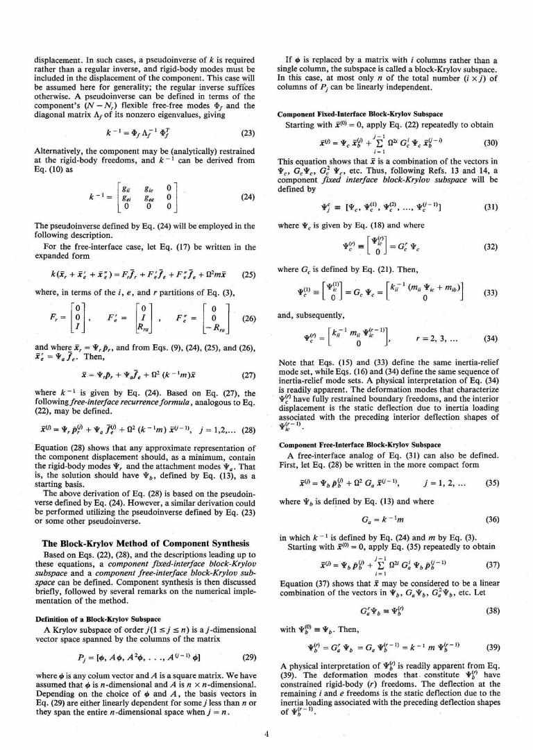
c i c t c t c tac tc t c t c t c t c t c tA. COMPONENTS AND COUPLED SYSTEM

ct ct ct a a b = r + e

B. TYPICAL COMPONENT WITH REDUNDANT BOUNDARY

Fig. 1 The component modal synthesis method distinguishes be-tween internal (/) and boundary (b} coordinates. Boundary coordi-nates are sometimes further divided into rigid-body (r) and excess (e),or redundant, coordinates.

mie mirmee mermre mrr

(3)

where the designations b, e, i, and r are defined below. Thetotal number of degrees of freedom of the component is N9while the number of degrees of freedom of the subsets b, e, /,and r are Nb, Ne, Nh and Nr9 respectively.

To relate the proposed block-Krylov method of componentsynthesis to previously described methods of componentsynthesis, the notation of Ref. 11, which reviews componentmodal synthesis methods, will be followed. Figure la shows acantilever beam divided into three components, while Fig. Ibidentifies the interior (i) and boundary (b) degrees of freedomof a typical component.§ If the component has rigid-bodyfreedom, the boundary coordinates may be subdivided intorigid-body (r) and redundant, or excess (e), coordinates.

In component modal synthesis the component displacementcoordinates jc are related to a reduced set of generalizedcoordinates p by the transformation

x = (4)

where ^ is a matrix whose columns are Ritz vectors, orso-called component modes. The types of modes that make up^ are: constraint modes (including rigid-body modes), attach-ment modes, and normal modes. Rigid-body modes, con-straint modes, and attachment modes of a beam componentare illustrated in Fig. 2 by ^r, ^c, and tya, respectively.Inertia-relief attachment modes, illustrated by ^rm in Fig. 2,are also employed in some versions of component modalsynthesis. In the block-Krylov method of component synthesisdescribed in this paper, component normal modes are replacedby a set of Krylov vectors.

The rigid-body modes ¥r of a component, e.g., see Fig. 2,can be defined by

(5)

where / is an r x r unit matrix.

§The "boundary" designation may be considered to apply to allcomponent freedoms where forces are applied or where adjacentcomponents are attached.

*m

Fig. 2 Examples of component modes of a beam element.

Redundant constraint modes ^fh are defined by

?/ kie kirk k?i *ee *ei

k k kKri Kre Kri

0Ree (6)

where / is an e x e unit matrix and R the reaction-forcematrices.

The subscript h is used because these are the constraintmodes used by Hurty in Ref. 1. A constraint mode is definedas the static deflection of a structure when a unit displacementis applied to one coordinate of a specified set of coordinates,while the remaining coordinates of that set are restrained andthe remaining degrees of freedom of the structure are forcefree. In Ref. 3, it was shown that the rigid-body modes ^fr andredundant constraint modes ^fh span the same subspace as aset of constraint modes ^fc defined by

(7)

(8)

By definition, the set of constraint modes is "staticallycomplete," i.e., the set is a basis for the linear space of all

» *»i r*fci = r °iw kbb\ [ I \ [Rbb\

That is, yc is given by

2

564 R. R. CRAIG JR. AND A. L. HALE J. GUIDANCE

possible deformations that result from static loads applied atthe boundary coordinates.

An attachment mode is defined as the static deflection of astructure when a unit force is applied at one coordinate of aspecified set of coordinates, while the remaining unrestrainedcoordinates are force free. When a structure has rigid-bodyfreedoms, either the structure can be restrained at an r-set ofcoordinates, or a set of inertia-relief attachment modes can bedefined as in Refs. 6-8. The former approach leads to thefollowing attachment modes ^fa defined for unit forces appliedat the excess (redundant) coordinates.

Let

U« kee\ ~ [get Seel

Then, from Eqs. (9) and (10)

0/

Rrn

0

(9)

(10)

(11)

It is shown in Refs. 7 and 11 that Va spans the same subspaceas *h. Specifically,

Then, letting

(12)

(13)

it is seen that tyb and ¥c span the same (Nr + Ne) subspace.Therefore, the set tyb is "statically complete."

Hintz7 defined a set of inertia-relief modes by the equation

kn kie kir^ if if*ei "*ee *-erk k kK,ri n,re /vr/.

0RemRrm

(14)

That is, the inertia-relief mode set ^fm is the set of staticdisplacements of the component restrained at all boundarycoordinates and loaded by the inertia forces resulting fromunit acceleration in each of the rigid-body modes of ^fr. Theinertia-relief modes ^fm are thus given by

kn00

(15)

Examples of ^rm modes are shown in the bottom two figures ofFig. 2. References 7 and 11 show that the inertia-relief modesym must be added to ^fb to form a "statically complete" modeset.

In Ref. 13, Craig proceeded to define a "sequence of inertiaattachment modes" by the recurrence relation

00

00

7 = 1,2,... (16)

and a similar set of inertia attachment modes based on ^fh. Aswill be shown later, the "component fixed-interface block-Krylov subspace" defined by Hale14 is the same space as thatspanned by the vectors defined by Craig.13

Derivation of Component Recurrence RelationsTo introduce component block-Krylov subspaces, it is

convenient to show first how these subspaces arise naturallywhen recursive solution procedures are applied to structuraldynamics problems. Over the years, various approximaterepresentations of the component displacement vector havebeen proposed in the form of Ritz expansions, as in Eq. (4).The block-Krylov approximation proposed in this paper issuggested by recurrence relations, which may be derived fromthe component equations of motion. Although both eigen-value and transient-response problems for the coupled systemare of interest in structural dynamics, it is simpler to deriverecurrence relations for the eigenproblem. In this case, thecomponent must satisfy the equation

(17)

where Q2 is an eigenvalue of the assembled system. Thecorresponding system natural frequency is Q, x is the portionof the system eigenvector within the component, and /constitutes boundary forces imposed on the component byadjacent components.

It is desired to manipulate Eq. (17) into forms in which xstands alone on the left-hand side. Two formulations areconsidered, depending on assumptions about the interface(boundary) degrees of freedom:

1) Interface degrees of freedom are constrained to be zero,i.e., a "fixed-interface" formulation.

2) All degrees of freedom, including those at the interface,are free, i.e., a "free-interface" formulation.

Note that although the assumptions above give the twoformulations their names, the interface coordinates are neither"fixed" nor "free" in the final system synthesis, but, rather,are subjected to inter element compatibility conditions.

Fixed-Interface Recurrence RelationsLet Eq. (17) be written in partitioned form as follows:

*The top portion can be solved for xt and the result combinedwith an identity for xb to give

0 0

It can safely be assumed that ku is nonsingular since thecomponents will be connected by either statically determinateor redundant connections.

Equation (19) can be written in the abbreviated form

x = xb (20)

where Vc is the constraint mode matrix defined by Eq. (8) andGc is defined by

Gc== 0 0 (21)

Based on Eq. (20), the following fixed-interface recurrenceformula may be defined.

O2 Gc j = 1,2,... (22)

Free-Interface Recurrence RelationsThis case is complicated by the fact that, when all of the

component degrees of freedom are free, the stiffness matrix kwill be singular if the component is free to undergo rigid-body

3


displacement. In such cases, a pseudoinverse of k is requiredrather than a regular inverse, and rigid-body modes must beincluded in the displacement of the component. This case willbe assumed here for generality; the regular inverse sufficesotherwise. A pseudoinverse can be defined in terms of thecomponent's (N — Nr) flexible free-free modes $y and thediagonal matrix Ay of its nonzero eigenvalues, giving

k-l = $ f A f l $J (23)

Alternatively, the component may be (analytically) restrainedat the rigid-body freedoms, and k~l can be derived fromEq. (10) as

Set0

8ieSee0

(24)

The pseudoinverse defined by Eq. (24) will be employed in thefollowing description.

For the free-interface case, let Eq. (17) be written in theexpanded form

k(xr + x'e + x "e ) = Frfr + F'Je + F"Je + tfnx (25)

where, in terms of the i, e, and r partitions of Eq. (3),

F = (26)

and where xr = Vrpr, and from Eqs. (9), (24), (25), and (26),*e =*afe- Then,

x = lm)x (27)

where k~l is given by Eq. (24). Based on Eq. (27), thefolio wing free-interface recurrence formula, analogous to Eq.(22), may be defined.

xU = *rp?+*aj™+&(k-lm)x«-l\ 7 = 1,2,... (28)

Equation (28) shows that any approximate representation ofthe component displacement should, as a minimum, containthe rigid-body modes *r and the attachment modes ¥a. Thatis, the solution should have ¥b, defined by Eq. (13), as astarting basis.

The above derivation of Eq. (28) is based on the pseudoin-verse defined by Eq. (24). However, a similar derivation couldbe performed utilizing the pseudoinverse defined by Eq. (23)or some other pseudoinverse.

The Block-Krylov Method of Component SynthesisBased on Eqs. (22), (28), and the descriptions leading up to

these equations, a component fixed-interface block-Krylovsubspace and a component free-interface block-Krylov sub-space can be defined. Component synthesis is then discussedbriefly, followed by several remarks on the numerical imple-mentation of the method.

Definition of a Block-Krylov SubspaceA Krylov subspace of ordery(l ^j ^ n) is ay-dimensional

vector space spanned by the columns of the matrix

(29)

where ̂ is any colum vector and A is a square matrix. We haveassumed that 0 is n -dimensional and A is n x n -dimensional.Depending on the choice of 0 and A, the basis vectors inEq. (29) are either linearly dependent for somey less than n orthey span the entire n -dimensional space wheny = n.

If 0 is replaced by a matrix with i columns rather than asingle column, the subspace is called a block-Krylov subspace.In this case, at most only n of the total number (/ xy) ofcolumns of Py can be linearly independent.

Component Fixed-Interface Block-Krylov SubspaceStarting with Jc(0) = 0, apply Eq. (22) repeatedly to obtain

_ _ J'~l • _ • _i — 1

This equation shows that x is a combination of the vectors in¥c, GCVC9 G* ¥c> etc. Thus, following Refs. 13 and 14, acomponent fixed interface block-Krylov subspace will bedefined by

where ^fc is given by Eq. (18) and where

where Gc is defined by Eq. (21). Then,

(31)

(32)

(33)

and, subsequently,r-l

. r = 2 , 3 , ... (34)

Note that Eqs. (15) and (33) define the same inertia-reliefmode set, while Eqs. (16) and (34) define the same sequence ofinertia-relief mode sets. A physical interpretation of Eq. (34)is readily apparent. The deformation modes that characterize¥^ have fully restrained boundary freedoms, and the interiordisplacement is the static deflection due to inertia loadingassociated with the preceding interior deflection shapes of

Component Free-Interface Block-Krylov SubspaceA free-interface analog of Eq. (31) can also be defined.

First, let Eq. (28) be written in the more compact form

where tyb is defined by Eq. (13) and where

Ga = k~ lm (36)

in which k ~l is defined by Eq. (24) and m by Eq. (3).Starting with Jc(0) = 0, apply Eq. (35) repeatedly to obtain

J — i—(A _ -^j. jn(f) i v^ O '̂' /~*' A!/ fi^'— ^ C\T\i= 1

Equation (37) shows that x may be considered to be a linearcombination of the vectors in ¥b9 Ga^rb9 Gfab9 etc. Let

=*b- Then»

= = Ga m

(38)

(39)

A physical interpretation of ^f(b is readily apparent from Eq.

(39). The deformation modes that constitute ^ haveconstrained rigid-body (r) freedoms. The deflection at theremaining i and e freedoms is the static deflection due to theinertia loading associated with the preceding deflection shapes

4


Finally, the free-interface block-Krylov subspace of order jmay be written as

Component SynthesisThe Ritz-type coordinate transformation (reduction) of

Eq. (4) leads to the reduced-order component model

JP + *P =

whereK

= *T k

(41)

(42)

As an example of the structure of the preceding reduced-order component matrices, let

then

00

0*23K33

(43)

(44)

where Ktj represents a submatrix. The zeroes in Eq. (44) resultfrom the &-orthogonality of the initial constraint modes in ^fcto all of the fixed-interface Krylov vectors which follow inGC*C9 etc. That is, from Eqs. (7) and (21),

*c k Gc 3 0 (45)

The form of K in Eq. (44) permits the direct stiffness method21

of component coupling to be used to enforce the interfacedisplacement compatibility equations for systems modeled byfixed-interface Krylov vectors.

To illustrate the procedure for coupling components toform a reduced-order system model, consider two compo-nents, a and /3, and let the uncoupled component matrices be

P =Pa o Ka 0

0 (46)

Compatibility of interface displacements, and other linearconstraint equations, may be collected to form the constraintequation

Cp =0 (47)

References 10 and 11 indicate how the constraint matrix C canbe used to define a coupling matrix S that, in turn, defines aset of independent system coordinates q, i.e.,

P = S q (48)

Thus, the coupled system equations of motion for freevibration of an undamped system are

Mq + Kg = 0

where

(49)

(50)

Additional terms for damping or external forcing followsimilarly.

1A damping matrix is included in Eq. (41) for completeness,although this is not to suggest that this is necessarily the best approachfor component synthesis for damped structures (e.g., see Ref. 20).

Remarks on Numerical ImplementationSeveral remarks on computing with block-Krylov vectors

are appropriate here:1) Numerical ill-conditioning may be encountered in form-

ing the column vectors spanning a Krylov subspace. Conse-quently, some type of orthogonalization procedure should beincorporated into a practical implementation of the method.Because limited precision of numerical computations, thecolumns of 0, A0, A20, ... can be linearly dependent, evenwhen they are theoretically independent. Therefore, in compu-tations it is appropriate to orthogonalize the vectors as theyare computed. This problem is accentuated when workingwith blocks of vectors. Fortunately, the problem is well-known and has been addressed in the literature on the Lanczosmethod (e.g., Ref. 22). Further research is being conducted onthis problem as it relates to component synthesis.

2) Computation of block-Krylov vectors should not bedone by inverting matrices. The expressions for Gc> Eq. (21),and Ga, Eq. (36), indicate the need for matrix inversion. Ofcourse, implementing these expressions requires only a singlefactorization of the appropriate stiffness matrix.

3) Although numerical examples suggest that only a fewblocks should suffice to give high accuracy in many applica-tions, the question of how many blocks to include to obtain agiven accuracy requires further research. A participationmatrix similar to the one defined by Nour-Omid and Clough16

may provide a suitable criterion for terminating the process ofcreating new blocks of Krylov vectors.

4) Although the question of how many blocks to includefor a given accuracy remains, the starting point is well-defined. It has been shown that constraint modes (attachmentmodes) serve as the starting blocks for the fixed-interface(free-interface) block-Krylov method. In fact, those compo-nent modal synthesis methods that compute approximatemodes via subspace iteration starting from random vectorsshould, instead, consider these blocks as a starting point fortheir iterations. This starting point is also appropriate to themultilevel iterative eigensolution methodology of Refs. 23 and24, from which Ref. 14 evolved.

Disturbability/Observability Properties ofBlock-Krylov Models

This section is devoted to discussing the attractive dis-turbability and observability properties of reduced-ordercomponent models based on the block-Krylov method.Indeed, the Ritz vectors of Eqs. (31) and (40) have a speciallinear-system-theoretic interpretation. Namely, they arisewhen considering disturbability and/or observability of inter-nal states from boundary disturbances/measurements. Hence,they are very good at representing component behavior whenthe primary interest is in the response of boundary degrees offreedom due to loadings at these degrees of freedom. Suchinterest is usually the case in launch vehicle/payload dynamic-loads models. Moreover, the special properties of the block-Krylov method suggest its importance to high-fidelity reduced-order modeling of actively controlled flexible structures, e.g.,large space structures.

General Disturbability/Observability CriteriaControllability/observability criteria for a linear, time-in-

variant system are well-known. Moreover, the concept ofdisturbability is related to that of controllability. Consider thesystem state equations written in first-order form:

*=Ax+Bf

y =

(51)

(52)

where x is the n-dimensional state vector, /is ap-dimensionalvector of inputs (controls or disturbances), and y is a#-dimensional vector of outputs (measurements). The under-

5


bar denotes a state matrix. The following are equivalent [e.g.,see Refs. 18 and 19 for (1) and (3)]:

1) The triple (A_ , B, C) is controllable and observable.2) The triple (A, B9 C) is disturbable and observable.3) The matrices Dn and On defined below have rank n .

matrices

O [CT, ATCT9 A2TCT, ..., -

(53)

(54)

In structural dynamics, the concept of disturbability is neededmore often than that of controllability. Herein, a system issaid to be disturbable if each and every state of the system canbe excited by an input disturbance. On the other hand,controllability refers to the existence of an input / that forces(controls) x(t) to the origin when starting from any finiteinitial state.

Disturbability/Observability Criteria for Undamped SubstructuresFor undamped substructures, which are governed by Eq.

(1), specific disturbability and observability criteria can bederived in terms of the mass and stiffness matrices. Forsimplicity, frequency-domain equations like Eq. (17) will beused in the derivation. Furthermore, a free-interface formula-tion with a nonsingular stiffness matrix k will be considered.

Let Eq. (17) be rewritten in the form

x = (I-&k-im)-lk-iFbfb (55)

where Fb is the (N'x Nb) boundary force distribution matrix

'.-[ifand let

(57)

where Cb is the (Nq x N) measurement appropriation matrix.A Taylor series solution for jc, based on Eq. (55), is

x = [/ + Q2 k - l m + (Q4/2) (k ~ l m)2 + -]k~ lFbfb (58)

This can be substituted into Eq. (57) to yield a Taylor seriesexpansion for the measurement vector, namely

(04/2) (k lFbfb (59)

The following proposition is based on Eqs. (58) and (59).

PropositionAn undamped Af-degree-offreedom component is com-

pletely disturbable from boundary excitation and completelyobservable from the observations of Eq. (57) if the respective

Table 1 Comparison of block-Krylov and CMS(Hurty-Craig-Bampton) methods: Free-free natural frequencies (Hz)

of example uniform beam

B-K7 = 10.0000.000

22.37862.978

145.139403.202

— .—

CMS/i =20.0000.000

22.38961.756

132.669326.761

—' —

B-K7=2

0.0000.000

22.37361.674

120.974202.521323.662528.553

CMSn = 40.0000.000

22.37461.678

120.988200.390200.305434.930

B-K/CMSy = l/ii=2

0.0000.000

22.37361.674

120.935210.686319.779517.137

FullFEM

0.0000.000

22.37361.674

120.911199.893298.666417.287

Dn = [k~lFb9 k~lFb9 ..., l Fb] (60)

-!<#] (61)

have rank N. If Dn does not have rank N, the disturbablesubspace is the linear space spanned by the columns of Dn.Similarly, if On does not have rank A/y the uriobservablesubspace is the null space of Oj.

The Appendix provides a proof of the disturbability part ofthe preceding proposition; a proof of the observability part issimilar.

Equations (60) and (61) define block-Krylov subspaces.They define the same subspace when all of the boundarydegrees of freedom are observed, i.e., when Cb=Fb. In thiscase, all of the degrees of freedom of block-Krylov reduced-order models are disturbable (observable) from disturbanceloads (observations) at component boundary degrees offreedom.

Numerical ExamplesTwo simple examples are presented in this section. They

both compare the new block-Krylov method with the fixed-interface component-modal-synthesis method.1'3 The firstexample considers a . simple ' free-free Bernoulli-Euler beamthat is divided into two components. The second example, Fig.3a, considers a free-free planar truss divided into threecomponents, Fig. 3b.

Free-Free Bernoulli-Euler BeamThe lower free- free natural frequencies for a uniform

Bernoulli-Euler beam are compared in Table 1. The beam isdivided into two components. The first component is 0.6 ofthe beam's length, and the second is the remaining 0.4 of thelength. In this example the bending stiffness, the total length,and the mass per unit length are all taken to be unity. The firstcomponent is modeled by six equal-length finite elements; thesecond is modeled by four equal-length elements. In the table,B-K denotes the block-Krylov results and CMS denotes theHurty-Craig-Bampton results. For B-K, /+! is the totalnumber of blocks; for CMS, n indicates the number offixed-interface modes included for each component. Sincethere are two degrees of freedom at the boundary of eachcomponent with the other, namely, a transverse displacementcoordinate and a rotational coordinate, each of the B-K blockshas two columns and each CMS component has two constraintmodes. Therefore, the assembled systems with natural fre-quencies given in columns 1 and 2 have 6 degrees of freedom(4 + 4-2 = 6), whereas those systems with frequencies given incolumns 3, 4, and 5 have 10 degrees of freedom(6 + 6-2=10).

A. UNDIVIDED B. DIVIDED INTO MAJOR COMPONENTS

Fig. 3 The accuracy of the component block-Krylov method iscompared to that of the CMS method using a planar truss antennamodel made of three components.

6


Table 2 Comparison Of block-Krylov and CMS (Hurty-Craig-Bampton) methods:Free-free natural frequencies (Hz) of example planar truss

B-K7 = 1

O.OOOOOOE + 0O.OOOOOOE + 0O.OOOOOOE + 01.953625E-22.205065E-24.923845E-27.273779E-27.626492E-21.550032E-11.617472E-1

CMS«=4


B-Ky = 2


CMSn- = 8


FullFEM


As seen by comparing the columns of Table 1, the newmethod compares very well with component modal synthesis.This is easily seen by comparing those system models obtainedby each method that have equal numbers of componentdegrees of freedom, i.e., by comparing columns 1 and 3 withcolumns 2 and 4, respectively. Moreover, by comparing thesecolumns with the last column, which contains the naturalfrequencies computed for the full-order (22 DOF) finite-element model, the block-Krylov method is seen to be slightlymore accurate for the lowest system modes, and the compo-nent-modal-synthesis method is seen to be slightly moreaccurate for the higher system modes. The fifth column showsnatural frequencies for a cross between the block-Krylov andthe modal-synthesis methods in which the block-Krylovmethod with j = 1 is supplemented by the two lowestfixed-interface component normal modes. From the results,no advantage is seen in this cross formulation.

Planar Truss-Antenna ModelThe truss structure shown in Fig. 3a is a planar model

representing a large truss-antenna. Although the model is notassociated with a specific antenna application, it is, neverthe-less, useful for numerical comparisons. It is divided into threecomponents as shown in Fig. 3b, namely, two feed masts anda reflector.

The natural frequencies of various assembled models aregiven in Table 2. Since the truss is planar, each finite-elementnodal point has two degrees of freedom. Hence, each of thethree components has four boundary degrees of freedom. Theblocks of the block-Krylov method then have four columns,whereas each component of the modal-synthesis method hasfour constraint modes. As noted previously, B-K denotes theblock-Krylov method with j + 1 being the number of blocks;CMS denotes the modal-synthesis method with n being thenumber of fixed-interface normal modes for each component.Assembled systems with natural frequencies given in columns1 and 2 have 18 degrees of freedom (DOF), whereas systemswith frequencies given in columns 3 and 4 have 30 DOF. Thefull-order finite-element model has 72 DOF. As indicatedearlier, the block-Krylov method is seen to have accuracycomparable to the modal-synthesis method. When comparingfrequencies for assembled systems with equal numbers ofdegrees of freedom, the block-Krylov method once againyields slightly more accurate lower system frequencies than themodal-synthesis method. The modal-synthesis method, on theother hand, yields slightly more accurate higher systemfrequencies than the block-Krylov method does. Finally, notethat the block-Krylov method accurately predicts the lowestseven nonzero system natural frequencies using only twoblocks for each component, i.e., withy = 1.

ConclusionsThe block-Krylov method is a simple and accurate method

for generating a set of component Ritz vectors for use incomponent synthesis. The block-Krylov Ritz vectors are

generated from easily derived recurrence relations. Thevectors span a subspace that is disturbable (observable) fromdisturbances (measurements) at the component's boundarycoordinates. Because of the disturbability and observabilityproperties, the method is particularly suited to applicationsrequiring high-fidelity reduced-order models. One such appli-cation area is that of large space structures. The accuracy ofthe fixed-interface block-Krylov method has been shown via anumerical example to be comparable to that of fixed-interfacecomponent modal synthesis. Since the computational expenseof the block-Krylov method is less than that for componentmodal synthesis, the block-Krylov method is preferable.

Appendix: Disturbability/Observability CriteriaThis appendix sketches a proof of the disturbability

proposition of Eq. (60); a proof of the observability proposi-tion is similar.

Note that Eq. (58) uses the fact that Jc can be written as alinear combination of the block matrices in Eq. (60) and aninfinite number of additional blocks. However, because x isonly TV-dimensional, there must eventually be a matrix

with columns that are linearly dependent on the combinedcolumn vectors of the preceding matrices 3>7 [/ = 0, 1, ...,(L -1)]. There must be such a matrix since there cannot bemore than TV linearly independent vectors in the TV-dimen-sional space. This implies that L <TV; in fact, it implies thatL <TV, where N=N/Nb9 or, if N/Nb is not an integer, thenthe next integer larger than N/Nb. Since the columns of <I>Ldepend linearly on the columns of $,- [/' = 0, 1,..., (L -1)], thefollowing expression for $L may be written,

=$ (A2)

where the //are appropriate_coefficient matrices. It followsthat each matrix $, (L <j <TV) depends linearly on the samecolumn vectors. Therefore, x is a linear combination of thecolumns of DL. That is, each excitation fb can only produce aresponse x dependent on the columns of DL. Moreover, alldirections (columns) can be excited; i.e., disturbed. Completedisturbability follows for those components for which therank of DL equals TV.

The disturbability/observability criteria of Eqs. (60) and(61) may also be related to the classical form of disturbabilityand observability in Eqs. (53) and (54), respectively. Bydefining the component state vector x to be

JC = (A3)

7


Equation (1) for an undamped structural component can bewritten in the form of Eq. (51), where

(A4)

where fs(t)=Fbfb(t) with Fb defined by Eq. (56). ExpandingEq. (53) using Eqs. (A4) yields

0 m~lFb 0

(A5)

A similar expression can be found for OL. Equation (A5)shows that x and jc are both spanned by the column vectors of

The above results are perhaps not fully appreciated withinthe structural dynamics and control of flexible structurescommunities. The results have important implications regard-ing the approximation of disturbable/observable subspaces bysubspaces of lower dimension. If, in the Rayleigh-Ritzmethod, a basis includes the column vectors of Z)0, noapproximation is introduced into solutions for given staticloads. This is not true, however, if the basis includes only areduced number of the columns of dL. The subspaces spannedby the columns of Z)/ are accurate from zero frequency at / = 0to progressively higher frequencies for / > 1, while thesubspaces df are accurate from infinity at / = 0 to progres-sively lower frequencies for / > 1. Since the structural modelitself is only accurate in the lower frequency region, reduced-order models based on the former are preferable.

] (A6)

If k is nonsingular, Eq. (A6) can be multiplied by (k~~lm)L toyield

DL = [ (A7)

whose blocks are defined in the same manner as the blocks inthe disturbability criterion, Eq. (60).

It remains to be shown that the columns of dL and DL spanthe same subspace. To show that they do, define

lFb (A8)

(A9)

ip $ _ (ir •rb > */ ~ v^

As before, there is an L < N such that

and such that each $y. (L </<A) depends linearly on thesame column vectors $/ [/ = 0, 1,..., (L — 1)]. It will be shownthat each $7 [0<y < (L — 1)] also depends linearly on thecolumns of ¥/ [/ = 0, 1, ... (L - 1)], and vice versa. Forbrevity, only the former is demonstrated here.

First, let $L be premultiplical by (m ~ lk)L to yield

L-l

i = 0(A10)

Equation (A 10) shows that <1>0 is a linear combination of all ofthe columns of ¥/ [0 <7 < (L — 1)]. Next, let $L be premulti-plied by (m ~ lk)L ~l to yield

L-2

/ = 0_ 2-0

/ =0

Thus, <!>! is also a linear combination of the vectors in ir/

[0 < i < (L — 1)]. The argument may be continued until it isshown that each $7 [/ = 0, 1,..., (L — 1)] is a linear combina-tion of the columns of the ^y [/' = 0, 1, ..., (L - 1)].Therefore, the linear space spanned by the columns of DL iscontained in the space spanned by the columns of dL . Similararguments show that the span of dL is contained in the span ofDL. Hence, dL and DL both span the same subspace. Hence,the disturbable subspace is spanned by the columns of dL andalso by the columns of DL . Of course, similar conclusions maybe found for observability. Finally, the disturbable andobservable subspaces are invariant under m~lk (for DL) and

AcknowledgmentsThe work of the first author was partially supported by

NASA Contract NAS9-17254 with the Lyndon B. JohnsonSpace Center. The interest of Dr. George Zupp and Mr. DavidHamilton is gratefully acknowledged.

Referencesy, W. C., "Dynamic Analysis of Structural Systems Using

Component Modes," AIAA Journal Vol. 3, April 1965, pp. 678-685.2Bamford, R. M., A Modal Combination Program for Dynamic

Analysis of Structures, TM 33-290, Jet Propulsion Lab., Pasadena,CA, July 1967.

3Craig, R. R., Jr., and Bampton, M. C. C., "Coupling ofSubstructures for Dynamic Analysis," AIAA Journal, Vol. 7, July1968, pp. 1313-1319.

4Benfield, W. A. and Hruda, R. F., "Vibration Analysis ofStructures by Component Mode Substitution," AIAA Journal, Vol.9, July 1971, pp. 1255-1261.

5MacNeal, R. H., "A Hybrid Method of Component ModeSynthesis," Computers and Structures, Vol. 1, 1971, pp. 581-601.

6Rubin, S., "Improved Component-Mode Representation forStructural Dynamic Analysis," AIAA Journal, Vol. 13, Aug. 1975,pp. 995-1006.

7Hintz, R. M., "Analytical Methods in Component Mode Synthe-sis," AIAA Journal, Vol. 13, Aug. 1975, pp. 1007-1016.

8Craig, R. R., Jr., and Chang, C-J., "On the Use of AttachmentModes in Substructure Coupling for Dynamic Analysis," Proceedingsof the AIAA 19th Structures, Structural Dynamics, and MaterialsConference, San Diego, CA, 1977, pp. 89-99.

9Dowell, E. H., "Free Vibration of an Arbitrary Structure in Termsof Component Modes," ASME Journal of Applied Mechanics, Vol.39, 1972, pp. 727-732.

10Craig, R. R., Jr., Structural Dynamics—An Introduction toComputer Methods, Wiley, New York, 1981.

nCraig, R. R., Jr., "A Review of Time-Domain and Frequency-Domain Component Mode Synthesis Methods j" Combined Experi-mental/Analytical Modeling of Dynamic Structural Systems,AMD—Vol. 67, American Society of Mechanical Engineering, NewYork, 1985, pp. 1-30; also International Journal of Analytical andExperimental Modal Analysis (to be published).

12Meirovitch L. and Hale, A. L., "On the Substructure SynthesisMethod," AIAA Journal, Vol. 19, July 1981, pp. 940-947.

13Craig, R. R., Jr., "A Study of Modal Coupling Methods,"Proceedings of the International Conference on Spacecraft Struc-tures, European Space Agency, Noordwijk, The Netherlands, 1985.

14Hale, A, L., "The Block-Krylov Method in Component Synthe-sis: An Alternative to Component Modes," AIAA Paper 86-0925,May 1986.

15Wilson, E. L., Yuan, M.-Wu, and Dickens, J. M., "DynamicAnalysis by Direct Superposition of Ritz Vectors," EarthquakeEngineering and Structural Dynamics, Vol. 10, 1982, pp. 813-821.

16Nour-Omid, B. and Clough, R. W., "Dynamic Analysis ofStructures Using Lanczos Coordinates," Earthquake Engineering andStructural Dynamics, Vol. 12, No. 4, 1984, pp. 565-577.

8


17Lu, X., "Dynamic Substructure Analysis Using Lanczos Vec-tors," First World Congress on Computational Mechanics, Austin,TX, Sept. 1986.

18Brogan, W. L., Modern Control Theory, Quantum Publishers,1974.

19Luenberger, D. G., Introduction to Dynamic Systems: Theory,Models, and Applications, Wiley, New York, 1979.

2°Craig, R. R., Jr., and Ni, Z., "Component Mode Synthesis forModel Order Reduction of Nonclassically-Damped Systems," AIAAGuidance, Navigation, and Control Conference, Monterey, CA, Aug.1987.

21 Bathe, K.-J., Finite-Element Procedures in Engineering Analysis,

Prentice-Hall, Englewood Cliffs, NJ, 1982.22Parlett, B. N. and Scott, S. N., "The Lanczos Algorithm with

Selective Orthogonalization," Mathematics of Computation, Vol. 33,1979, pp. 217-238.,

23Hale, A. L. and Meirovitch, L., "A Procedures for ImprovingDiscrete Substructure Representation in Dynamic Synthesis," AIAAJournal, Vol. 20, Aug. 1982, pp. 1128-1136.

24Hale, A. L. and Warren, L. V., "Concepts of a General Substiruc-turing System for Structural Dynamics Analyses," Journal ofVibration, Acoustics, Stress, and Reliability in Design, Vol. 107, No.1, 1985, pp. 2-12.

Recommended Reading from the AIAAProgress in Astronautics and Aeronautics Series .

Dynamics of Flames and ReactiveSystems and Dynamics of Shock Waves,Explosions, and DetonationsJ. R. Bowen, N. Manson, A. K. Oppenheim, and R. I. Soloukhin, editors

The dynamics of explosions is concerned principally with the interrelationship betweenthe rate processes of energy deposition in a compressible medium and its concurrentnonsteady flow as it occurs typically in explosion phenomena. Dynamics of reactivesystems is a broader term referring to the processes of coupling between thedynamics of fluid flow and molecular transformations in reactive media occurring inany combustion system. Dynamics of Flames and Reactive Systems covers prehnixedflames, diffusion flames, turbulent combustion, constant volume-combustion, spraycombustion nonequilibrium flows, and combustion diagnostics. Dynamics of ShockWaves, Explosions and Detonations covers detonations in gaseous mixtures, detona-tions in two-phase systems, condensed explosives, explosions and interactions.

Dynamics of Flames andReactive Systems1985 766 pp. illus., HardbackISBN 0-915928-92-9AIAA Members $54.95Nonmembers $84.95Order Number V-95

Dynamics of Shock Waves,Explosions and Detonations

1985 595 pp., illus. HardbackISBN 0-915928-91-4

AIAA Members $49.95Nonmembers $79.95Order Number V-94

TO ORDER: Write AIAA Order Department, 370 L'Enfant Promenade, S.W., Washington, DC 20024. Please includepostage and handling fee of $4.50 with all orders. California and D.C. residents must add 6% sales tax. All ordersunder $50.00 must be prepaid. All foreign orders must be prepaid.

9

block-krylov component synthesis method for structural

Documents