Department of Economics

Working Paper

Block Bootstrap Prediction Intervals for Autoregression

Jing Li

Miami University

2013

Working Paper # - 2013-02

Block Bootstrap Prediction Intervals for Autoregression

Jing Li∗

Abstract

This paper provides evidence that the principle of parsimony can be extended to

interval forecasts. We propose new prediction intervals based on parsimonious au-

toregressions. The serial correlation in the error term is accounted for by the block

bootstrap. The proposed intervals generalize the i.i.d bootstrap intervals by allowing

for serially correlated errors. Simulations show the proposed intervals have superior

performance when the serial correlation in the error term is strong and when forecast

horizon is short. By applying the proposed intervals to U.S. inflation rate, we highlight

a tradeoff between preserving correlation and adding variation.

Keywords: Forecast; Block Bootstrap; Stationary Bootstrap; Prediction Intervals;

Principle of Parsimony

EconLit Subject Descriptors: C15; C22; C53

∗Jing Li, Department of Economics, Miami University, Oxford, OH 45056, USA. Phone: 001.513.529.4393,Fax: 001.513.529.6992, Email: lij14@miamioh.edu.

1

1. Introduction

It is well known that a parsimonious model may produce superior out-of-sample point fore-

casts than a complicated model. The main contribution of this paper is to examine whether

the principle of parsimony can be extended to interval forecasts. The proposed block boot-

strap prediction intervals (BBPI) are based on a parsimonious first order autoregression.

By contrast, the i.i.d or standard bootstrap prediction intervals developed by Thombs and

Schucany (1990) (called TS intervals thereafter) are based on the autoregression of order p,

where p can be large. The TS intervals assume the error term is independent. Thus the

BBPI generalize the TS intervals by allowing for serially correlated errors.

A largely overlooked fact is that the principle of parsimony is forgone by the classical Box-

Jenkins prediction intervals and the TS intervals. Both require serially uncorrelated error

terms, and therefore dynamically complete models1. Usually the Breusch-Godfrey type test

is conducted to ensure the adequacy of model. On the other hand, when the goal is the

point forecast, the models selected by criteria of AIC and BIC are typically parsimonious,

but not necessarily adequate, see Enders (2009).

The proposed intervals do not require dynamically complete models. Unlike the Box-

Jenkins intervals, non-normality can be automatically accounted for. This is because the

block bootstrap is employed to obtain the empirical conditional distribution, which can be

non-normal, of the out-of-sample forecast. More explicitly, the block bootstrap redraws with

replacement random blocks of consecutive residuals of a parsimonious (short) autoregres-

sion. The blocking is intended to preserve the time dependence structure in the error term.

By contrast, the TS intervals entail the i.i.d bootstrap of Efron (1979) that resamples in-

dividual residual. The i.i.d bootstrap works well in the independent setup. To satisfy the

independence of the error term, a complicated (long) autoregression is needed for the TS

intervals.

1See the footnote page.

2

This paper also applies the bootstrap method to direct forecasts. There are two ways to

obtain the h-step forecast. The first is to run just one autoregression, and then compute the

h-step forecast based on (h− i)-step forecasts. We call these iterated forecasts. The second

way is to run a set of direct autoregressions. They all use yt as the dependent variable, but

the regressors are different. In the simplest case, the only regressor is yt−1 in the first direct

regression, yt−2 in the second direct regression, and so on. We call these direct forecasts.

This paper considers both forecasts.

There are three steps to construct the BBPI. In step one the AR(1) regression is esti-

mated by ordinary least squares (OLS), and the residual is saved. In step two a backward

AR(1) regression is fitted, and random blocks of residuals are used to generate the bootstrap

replicate. In step three the bootstrap replicate is used to run the AR(1) regression again

and random blocks of residuals in step one are used to compute the bootstrap out-of-sample

forecast. After repeating steps two and three many times, the BBPI are determined by the

percentiles of the empirical distribution of the bootstrap forecast. We discuss technical issues

such as correcting the bias of autoregressive coefficients, selecting the block size (length),

choosing between overlapping and non-overlapping blocks and using the stationary bootstrap

that sets the block size as random.

Monte Carlo experiment compares the average coverage rate of the BBPI to the TS

intervals. There are two key findings. The first is that the BBPI dominate when the error

term shows strong serial correlation after yt−1 being controlled for. The second is that the

BBPI always outperform the TS intervals for the one-step forecast. For longer forecast

horizon, it is possible that the TS intervals perform better. Our findings highlight a tradeoff

between preserving correlation and adding variation. The block bootstrap achieves the

former but sacrifices the latter. This tradeoff is also illustrated when we apply the BBPI to

the U.S. monthly inflation rate.

The literature on the bootstrap prediction intervals is growing fast. Important works

3

include Thombs and Schucany (1990), Masarotto (1990), Grigoletto (1998), Clements and

Taylor (2001), Kim (2001), and Kim (2002). The block bootstrap and stationary bootstrap

are fully developed by Kunsch (1989) and Politis and Romano (1994). See Stock and Watson

(1999) and Stock and Watson (2007) for more discussion about forecasting the U.S. inflation

rate. The remainder of the paper is organized as follows. Section 2 specifies the BBPI.

Section 3 conducts the Monte Carlo experiment. Section 4 provides an application, and

Section 5 concludes.

2. Block Bootstrap Prediction Intervals

Iterated Block Bootstrap Prediction Intervals

Let yt, t ∈ Z be a strictly stationary and weakly dependent time series with mean of zero.

In practice yt may represent the demeaned, differenced, detrended or deseasonalized series.

The goal is to find the prediction intervals for future values (yn+1, yn+2, . . . , yn+h), where h

is the maximum forecast horizon, after observing Ω = (y1, . . . , yn). This paper focuses on

the bootstrap prediction intervals because (i) they do not assume that the distribution of

yn+i conditional on Ω is normal, and (ii) the bootstrap intervals can automatically take into

account the sampling variability of the estimated coefficients.

The TS intervals of Thombs and Schucany (1990) are based on a “long” p-th order

autoregression:

yt = ψ1yt−1 + ψ2yt−2 + . . .+ ψpyt−p + et. (1)

The TS intervals assume the error et is independent of (or at least uncorrelated with)

et−j, ∀j = 0. This assumption requires that the model (1) be dynamically adequate. In

other words, sufficient number of lagged values should be included. It is not uncommon that

in practice the final model can be complicated, which is inconsistent with the principle of

parsimony. Actually the model (1) is just a finite-order approximation if the true process is

4

ARMA process that has AR(∞) representation. In theory the error term et can be serially

correlated no matter how large p is. This implies the independent assumption can be too

restrictive.

This paper relaxes the assumption of independent errors, and proposes the block boot-

strap prediction intervals (BBPI) based on a “short” autoregression. Consider the AR(1)

model, the most parsimonious autoregression

yt = ϕ1yt−1 + vt. (2)

The error vt is allowed to be serially correlated, so Model (2) can be inadequate. Nevertheless,

the serial correlation in vt should be utilized to improve the forecast. Toward that end the

block bootstrap later will be applied to the residual

vt = yt − ϕ1yt−1, (3)

where ϕ1 is the coefficient estimated by OLS.

But first, any bootstrap prediction intervals should account for the sampling variability

of ϕ1. This is accomplished by running repeatedly the regression (2) using the bootstrap

replicate, a pseudo time series. Following Thombs and Schucany (1990) we generate the

bootstrap replicate using the backward representation of the AR(1) model

yt = θ1yt+1 + ut. (4)

Note that the regressor is lead not lag. Denote the OLS estimate by θ1, and the residual by

ut :

ut = yt − θ1yt+1, (5)

5

then one series of the bootstrap replicate (y∗1, . . . , y∗n) is computed in a backward fashion as

(starting with the last observation, then moving backward)

y∗n = yn, y∗t = θ1y

∗t+1 + u∗t , (t = n− 1, . . . 1). (6)

By using the backward representation we can ensure the conditionality of AR forecasts on

the last observed value yn. Put differently, all the bootstrap replicate series have the same

last observation, y∗n = yn. See Figure 1 of Thombs and Schucany (1990) for an illustration

of this conditionality.

In equation (6) the randomness of the bootstrap replicate comes from the pseudo error

term u∗t , which is obtained by the block bootstrap as follows:

1. Save the residual of the backward regression ut given in (5).

2. Let b denote the block size (length). The first (random) block of residuals is

B1 = (ui1, ui1+1, . . . , ui1+b−1), (7)

where the index number i1 is a random draw from the discrete uniform distribution

between 1 and n−b+1. For instance, let b = 3 and suppose a random draw yields i1 =

20, then B1 = (u20, u21, u22). In this example the first block contains three consecutive

residuals starting from the 20th observation. By redrawing the index number with

replacement we can obtain the second block B2 = (ui2, ui2+1, . . . , ui2+b−1), the third

block B3 = (ui3, ui3+1, . . . , ui3+b−1), and so on. We stack up these blocks until the

length of the stacked series becomes n. u∗t denotes the t-th observation of the stacked

series.

Resampling blocks of residuals is intended to preserve the serial correlation of the error

term in the parsimonious model. Generally speaking, the block bootstrap can be applied

6

to any weakly dependent stationary series. Here it is applied to the residual of the short

autoregression. By contrast, the TS intervals resample the individual residual of a long

autoregression.

There are several issues. The first is how to determine the block size b. There is no definite

answer due to a tradeoff between correlation and variation. We face the same tradeoff when

choosing between the block bootstrap and the i.i.d bootstrap. Longer block (bigger b) can

capture more serial correlation. But longer block also reduces the variation in the bootstrap

replicate because (i) the total number of blocks falls and (ii) the chance of overlapping blocks

rises. The general rule is that b should rise when serial correlation gets stronger, or when the

sample size grows. For our purpose this issue may not be as important as it appears, because

simulations will show the superiority of the BBPI over the TS intervals may be insensitive

to b.

Alternatively, one may resample blocks with random sizes, where the block size follows

a geometric distribution. That is the main idea of the stationary bootstrap suggested by

Politis and Romano (1994). More explicitly, the distribution of b is specified as

P (b = j) = p(1− p)j, (j = 0, 1, 2, ...). (8)

When p rises, the probability of generating small values of b also rises. Notice that using

stationary bootstrap does not solve the problem completely. Now the new problem is how to

select the probability parameter p. The rule is we should let p fall when the serial correlation

gets stronger. In the simulation we replace b = 0 with b = 1 if that happens.

The second issue is overlapping vs non-overlapping blocks. The algorithm above indi-

cates the blocks are possibly overlapping. For example, B1 partially overlaps with B2 when

i1 < i2 < i1 + b. To generate non-overlapping blocks, we need to randomly redraw with

7

replacement the index numbers i1, i2, . . . from the below set:

1, 1 + b, 1 + 2b, . . . , 1 + kb, (9)

where k ≤ nb− 1. Note there are gaps between the values in (9), which ensure the blocks

are not overlapping. When b rises, using non-overlapping blocks generates less randomness

than overlapping blocks, simply because k falls and there are fewer values left in (9). We

will revisit this issue in the simulation. See Andrews (2004) for a discussion in the context

of hypothesis testing.

Finally, it is not required that the modulo of dividing n by b be zero. Only a portion of

the last block is included in the stacked series with nonzero modulo. For example, it is ok

that the length of stacked series is 100, b = 3, and 100 is not a multiple of 3. A total of 34

blocks are drawn, but only the first observation of the 34-th block is included in the stacked

series.

After generating the bootstrap replicate series using (6), next we refit the model (2) using

the bootstrap replicate (y∗2, . . . , y∗n). Denote the newly estimated coefficient (called bootstrap

coefficient) by ϕ∗1. Then we can compute the iterated block bootstrap l-step forecast y∗n+l as

y∗n = yn, y∗n+l = ϕ∗

1y∗n+l−1 + v∗l , (l = 1, . . . , h) (10)

where the pseudo error v∗l is obtained by block bootstrapping the residual (3). For example,

let h = 8, b = 4. Then two blocks of residuals (3) are randomly drawn, and they are B1 =

(vi1, vi1+1, vi1+2, vi1+3), B2 = (vi2, vi2+1, vi2+2, vi2+3). Then v∗l in equation (10) is the l-th

observation of the stacked series

v∗l hl=1 = vi1, vi1+1, vi1+2, vi1+3, vi2, vi2+1, vi2+2, vi2+3. (11)

8

The ordering of B1 and B2 in the stacked series (11) does not matter. It is the ordering of

the observations within each block that matters. That within-block ordering preserves the

temporal structure.

Notice that the block bootstrap has been invoked twice: first it is applied to ut given

in (5), then applied to vt given in (3). The first application is to add randomness to the

bootstrap replicate y∗t , which is used to rerun the autoregression and simulate the sampling

variability of the estimated coefficient. The second application is to randomize the predicted

value y∗n+l. The block size when resampling vt is the same as ut since (4) and (2) share the

same structure of serial correlation, see Box et al. (2008).

To get the BBPI, we need to generate C series of the bootstrap replicate using (6), fit

the model (2) using the C bootstrap replicate series, and use (10) to obtain a series of the

iterated block bootstrap l-step forecasts

y∗n+l(i)Ci=1 (12)

where i is the index. The l-step iterated BBPI at the α nominal level are given by

l − step Iterated BBPI (IBBPI) =

[y∗n+l

(1− α

2

), y∗n+l

(1 + α

2

)](13)

where y∗n+l

(1−α2

)and y∗n+l

(1+α2

)are the

(1−α2

)100-th and

(1+α2

)100-th percentiles of the

empirical distribution of y∗n+l(i)Ci=1. Throughout this paper we let α = 0.90. To avoid the

discreteness problem, one may let C = 999, see Booth and Hall (1994). In this paper we use

C = 1000 and find no qualitative difference.

Basically we apply the percentile method of Efron and Tibshirani (1993) to construct the

BBPI. De Gooijer and Kumar (1992) emphasize the percentile method performs well when

the conditional distribution of the predicted values is unimodal. In preliminary simulation

we conduct the DIP test of Hartigan and Hartigan (1985) and find that the distribution is

9

indeed unimodal. Hall (1988) discusses other percentile methods.

Bias-Corrected Prediction Intervals

It is well known that the autoregressive coefficient estimated by OLS can be biased, see

Shaman and Stine (1988) for instance. That implies the BBPI (13) can be improved by

correcting the bias. Following Kilian (1998) we generate D series of the bootstrap replicate

using (6), then refit the backward regression (4) using these bootstrap replicate series and

get a series of bootstrap backward coefficients θ∗1(i)Di=1. Next compute the bias-corrected

coefficient, bias-corrected residual and bias-corrected bootstrap replicate as

θc1 = 2θ1 −D−1

D∑i=1

θ∗1(i), (14)

uct = yt − θc1yt+1, (15)

yc∗n = yn, yc∗t = θc1y

c∗t+1 + uc∗t , (t = n− 1, . . . 1), (16)

where uc∗t is obtained by block bootstrapping uct . Finally, refit the model (2) using the bias-

corrected bootstrap replicate yc∗t and compute the bias-corrected bootstrap forecast as

yc∗n = yn, yc∗n+l = ϕc∗

1 yc∗n+l−1 + v∗l , (l = 1, . . . , h), (17)

where v∗l is obtained by block bootstrapping vt (3). The bias-corrected BBPI are determined

by the percentiles of the distribution of yc∗n+l.

Actually we can go one step further by bias correcting the residual v of (3). To do so, we

need to use the D series of the bootstrap replicate to refit the forward regression (2). After

obtaining a series of bootstrap forward coefficients ϕ∗1(i)Di=1, compute the bias-corrected

10

forward coefficient and bias-corrected forward residual as

ϕc1 = 2ϕ1 −D−1

D∑i=1

ϕ∗1(i), (18)

vct = yt − ϕc1yt−1. (19)

Then the twice bias-corrected bootstrap forecast is computed as

y2c∗n = yn, y2c∗n+l = ϕc∗

1 y2c∗n+l−1 + vc∗l , (l = 1, . . . , h), (20)

where vc∗l is obtained by block bootstrapping vct (19).

Equation (20) makes it clear that vc∗l has direct effect on the bootstrap forecast, while

uc∗t only has an indirect effect through ϕc∗1 . So we conjecture that bias correcting the forward

residual vt is more important than the backward residual ut. This conjecture will be verified

by the simulation. In practice one may also apply the stationary correction recommended

by Kilian (1998) to ensure the series of bootstrap replicate y∗t is stationary.

Direct Block Bootstrap Prediction Intervals

We call the BBPI (13) iterated because the forecast is computed in an iterative fashion: in

(10) the previous step forecast y∗n+l−1 is used to compute the next step y∗n+l. Alternatively, we

can use the bootstrap replicate (y∗1, . . . , y∗n) to run a set of direct regressions using only one

regressor. In total there are h direct regressions. More explicitly, the l-th direct regression

uses y∗t as the dependent variable and y∗t−l as the independent variable. Denote the estimated

direct coefficient by ρ∗l . The residual is computed as

ηt,l = y∗t − ρ∗l y∗t−l. (21)

11

Then the direct bootstrap forecast is computed as

yd∗n+l = ρ∗l yn + η∗l (22)

where η∗l is a random draw with replacement from the empirical distribution of ηt,l. The

l-step direct BBPI at the α nominal level are given by

l − step Direct BBPI (DBBPI) =

[yd∗n+l

(1− α

2

), yd∗n+l

(1 + α

2

)](23)

where yd∗n+l

(1−α2

)and yd∗n+l

(1+α2

)are the

(1−α2

)100-th and

(1+α2

)100-th percentiles of the

empirical distribution of yd∗n+l(i)Ci=1.

There are other ways to obtain the direct prediction intervals. For example, the bootstrap

replicate (y∗1, . . . , y∗n) can be generated based on the backward form of direct regression. It

is also possible to bias correct the coefficient in the direct regression. Ing (2003) compares

the mean-squared prediction errors of the iterated and direct point forecasts. In the next

section we will compare the iterated and direct BBPIs.

3. Monte Carlo Experiment

Error Distributions

This section compares the performances of various bootstrap prediction intervals using the

Monte Carlo experiment. First we investigate the distribution of error term. Following

Thombs and Schucany (1990), the data generating process (DGP) is a stationary AR(2)

process:

yt = ϕ1yt−1 + ϕ2yt−2 + ut (24)

where ϕ1 = 0.75, ϕ2 = −0.5, t = 1, . . . , 55. The error ut follows an independently and iden-

tically distributed process. Three error distributions are considered: the standard normal

12

distribution, the exponential distribution with mean of 0.5, and mixed normal distribution

0.9N(−1, 1) + 0.1N(9, 1). The exponential distribution is skewed; the mixed normal distri-

bution is bimodal and skewed. All distributions are centered to have zero mean.

We compare three bootstrap prediction intervals. The iterated block bootstrap prediction

intervals (IBBPI) are based on the “short” AR(1) regression (2) and its backward form (4).

The TS intervals of Thombs and Schucany (1990) are based on the “long” AR(2) regression

(24) and its backward form. Because we know the true DGP is AR(2), the error terms in

the AR(1) regression are serially correlated, while the errors are uncorrelated in the AR(2)

regression. Finally the direct block bootstrap prediction intervals (DBBPI) are based on

a series of first order direct autoregressions. Each bootstrap prediction intervals are based

on the empirical distribution of 1000 bootstrap forecasts. That is, we let C = 1000 in (12)

for the IBBPI, and so on. For the IBBPI and DBBPI the block size b is set to 4. The TS

intervals use the i.i.d bootstrap, so block size is irrelevant.

The first 50 observations (n = 50) are used to run the regression. Then we evaluate

whether the last 5 observations are inside the corresponding prediction intervals. In other

words, we focus on out-of-sample forecasting. The main criterion of comparing performance

is the average coverage rate (ACR) given as:

ACR(h) = m−1

m∑i=1

1(yn+h ∈ Prediction Intervals) (25)

where 1( .) denotes the indicator function. The number of iteration is set as m = 5000. We

find no qualitative difference if using m = 20000. The forecast horizon h ranges from 1 to 5.

The nominal coverage α is 0.90. The intervals whose ACR is closest to 0.90 are deemed the

best.

Figure 1 plots the ACR against h when the error distribution varies. The ACRs of the

IBBPI, TS intervals and DBBPI are denoted by circle, square and star, respectively. In

13

the leftmost graph the error follows the standard normal distribution. It is shown that the

ACR of the IBBPI is closest to the nominal coverage 0.90, followed by the TS intervals. The

DBBPI have the worst performance. For instance, when h = 5, the IBBPI have ACR of

0.883, the TS intervals have ACR of 0.854, and the DBBPI have ACR of 0.829.

The ranking remains largely unchanged when the errors follow the exponential and mixed

normal distributions, shown in the middle and rightmost graphs. Overall, Figure 1 indicates

that (i) the IBBPI have the best performance, and (ii) the DBBPI have the worst perfor-

mance. Finding (ii) is consistent with previous works such as Ing (2003) which shows the

iterated point forecast outperforms the direct point forecast. Finding (i) is new, and may be

explained by the fact that the IBBPI are based on the parsimonious model. By comparing

the three graphs, we see no big change in ACR when the error distribution varies. This is

expected because all intervals are bootstrap intervals that do not assume normality.

Autoregressive Coefficients

Now we consider varying autoregressive coefficients in the DGP (24):

ϕ1 = 0.75, ϕ2 = −0.5 (stationary AR(2)) (26)

ϕ1 = 1.0, ϕ2 = −0.24 (stationary AR(2)) (27)

ϕ1 = 1.2, ϕ2 = −0.2 (non-stationary AR(2)) (28)

where t = 1, . . . , 55 and ut ∼ iidn(0, 1). The leftmost graph in Figure 2 looks similar to

that in Figure 1 since the same DGP is used. In the middle graph we see no difference

in the ranking. The rightmost graph is interesting. In this case the sum of autoregressive

coefficients is 1.2 − 0.2 = 1. So the data are nonstationary (one characteristic root is 1),

violating the assumption of stationarity. This violation leads to distortion in the coverage

rate, particularly when h is big. For example, at h = 5, the ACR of the IBBPI is between 0.85

14

and 0.88 when data are stationary, but close to 0.76 when data are nonstationary. In light

of this we recommend applying the prediction intervals to the differenced data if the data

contain unit roots. We also see the direct intervals are the best when data are nonstationary.

This may be due to the fact that the direct intervals are based on the direct regression.

Sample Sizes

Figure 3 is concerned with the sample size. The DGP is (24) with ϕ1 = 0.75, ϕ2 = −0.5,

ut ∼ iidn(0, 1). Three sample sizes are used for in-sample fitting: n = 30, n = 60 and

n = 100. From Figure 3 we see as the sample size rises, the ACR lines in most cases move

closer to the nominal level 0.90. Therefore rising sample size improves the performance of

all intervals.

Block Sizes

Now we focus on the IBBPI, and investigate how the block size affects performance. The

DGP is (24) with t = 1, . . . , 55, ut ∼ iidn(0, 1). The coefficients are given in (26), (27) and

(28). There are two findings from Figure 4. First, using the block size of one (i.e., the i.i.d

bootstrap, denoted by circle) leads to the worst performance. The second finding is that the

difference between using the block sizes of three (denoted by square) and five (denoted by

star) is marginal in most cases. This suggests that the performance of the BBPI may be

insensitive to the block size. As long as blocks are used, the block size may be a secondary

issue.

Block Bootstrap Intervals vs Stationary Bootstrap Intervals

Instead of using the block of a fixed size, we can employ the stationary bootstrap that

resamples blocks of random sizes. Using the same DGP as Figure 4, Figure 5 compares the

(iterated) block bootstrap prediction intervals (BBPI) with b = 4 (denoted by circle) to the

15

stationary bootstrap prediction interval (SBPI) of the block size that follows the geometric

distribution with parameter p = 0.3 (denoted by square). Figure 5 shows that in most cases

the difference between the two intervals is not substantial. No one can dominate the other.

Overall, it is safe to say the stationary bootstrap, which depends on the choice of p, is an

alternative to the block bootstrap, which depends on the choice of b.

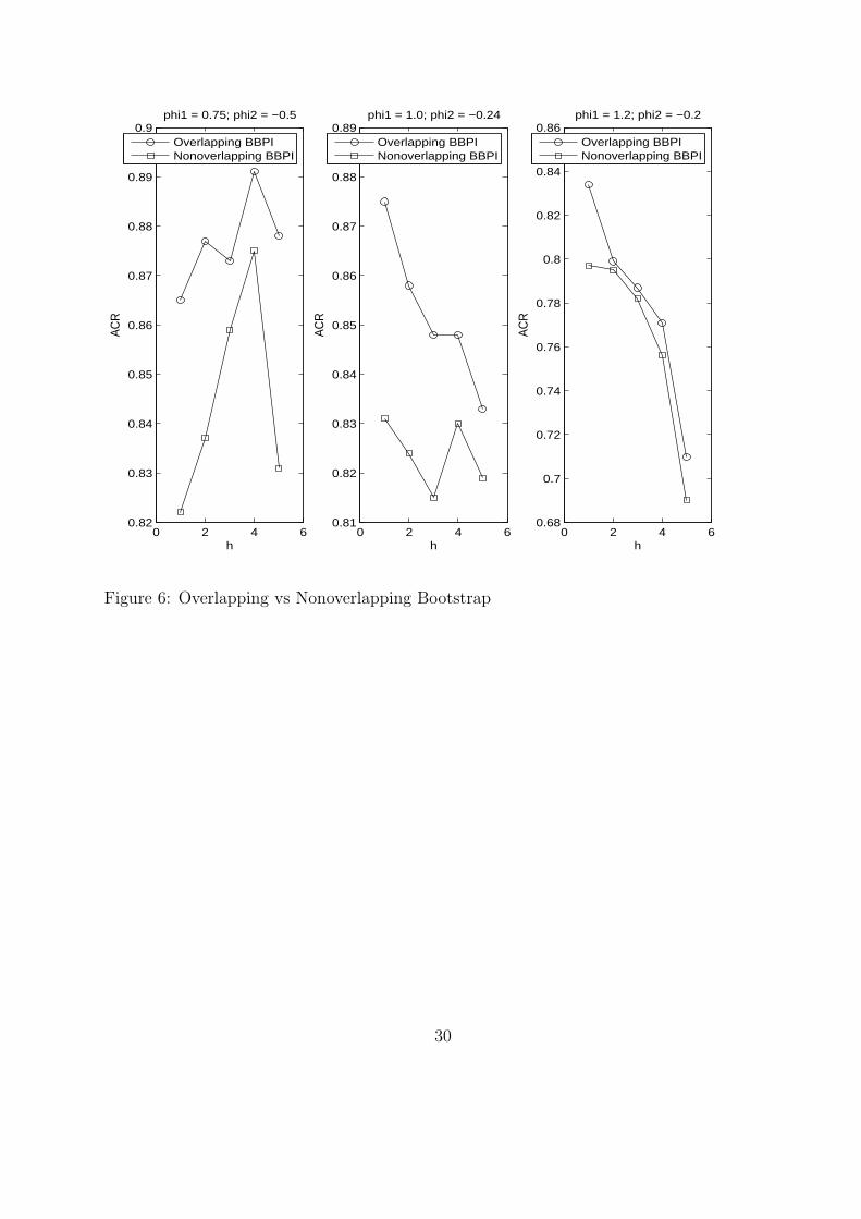
Overlapping vs Non-overlapping Blocks

Using the same DGP as Figure 4, Figure 6 compares the (iterated) block bootstrap prediction

intervals using overlapping (denoted by circle) and non-overlapping (denoted by square)

blocks. The block size is 4. We see that using overlapping blocks yields better performance

than non-overlapping blocks. The reason may be that overlapping blocks can produce more

variation in the bootstrap replicate than non-overlapping blocks.

Bias Correction

Now we investigate whether correcting the bias of autoregressive coefficient can improve the

performance of intervals. Figure 7 compares the iterated block bootstrap prediction intervals

based on (10), (17) and (20). Basically (10) does not correct the bias; (17) only corrects the

bias of θ1, the coefficient in the backward regression; (20) corrects both θ1 and ϕ1, the latter

is the coefficient in the forward regression. In Figure 7 these intervals are denoted by circle

(no bias correction, or no BC), square (BC Once) and star (BC Twice), respectively. The

DGP is the same as Figure 4.

From Figure 7 it is clear that the BC Twice intervals have the best performance. It

appears that correcting the coefficient in the backward regression alone results in almost no

improvement. In light of this we conclude that bias-correcting the coefficient in the forward

model (2) is far more important than bias-correcting the coefficient in the backward model

(4). Another finding is that bias-correcting coefficients pushes the coverage rate up toward

16

the nominal 0.90. This indicates that at least part of the downward bias in coverage rate we

see in all graphs is caused by the bias of autoregressive coefficients.

Principle of Parsimony

So far the DGP has been the AR(2) model (24). Next we change the DGP to an ARMA(1,1)

process

yt = ϕyt−1 + ut + θut−1 (29)

where t = 1, . . . , 55 and ut ∼ iidn(0, 1). In theory for this DGP there exists AR(∞) repre-

sentation. Thus the AR(p) regression is finite-order approximation.

We verify the principle of parsimony in three ways. Figure 8 compares the iterated block

bootstrap prediction intervals based on the AR(1) regression, to the TS intervals based on

the AR(2) regression (TS2, denoted by diamond), the AR(3) regression (TS3, denoted by

square) and the AR(4) regression (TS4, denoted by star). For the TS intervals we do not

check whether the residual is serially correlated. That job is left to Figure 9.

Figure 8 uses three sets of ϕ and θ. Regardless of the coefficient, the block bootstrap

intervals have the best performance. When the autoregression becomes longer, the corre-

sponding TS intervals show worse performance. This is the first evidence that the principle

of parsimony may work for interval forecasts.

The second evidence is presented in Figure 9, where the TS intervals are based on the

autoregression whose order is determined by the Breusch-Godfrey test. The Breusch-Godfrey

test is appropriate since the regressors are lagged dependent variables. We start from the

AR(1) regression. If the residual passes the Breusch-Godfrey test, then the AR(1) regression

is chosen for constructing the TS intervals. Otherwise we change to the AR(2) regression,

apply the Breusch-Godfrey test again, and so on. In the end, the TS intervals are based on

an adequate autoregression with serially uncorrelated errors.

17

In the leftmost graph of Figure 9, ϕ = 0.4, θ = 0.2. We see the iterated block bootstrap

intervals outperform the TS intervals when h equals 1 and 2. For greater h their ranking

reverses. In the middle and rightmost graphs, more serial correlation is induced as θ rises

from 0.2 to 0.6, and as ϕ rises from 0.4 to 0.9. In those two graphs the BBPI dominate the

TS intervals.

The fact that the ranking of the BBPI and TS intervals switches in the leftmost graph

indicates a tradeoff between preserving serial correlation and adding variation. Remember

that the BBPI use the block bootstrap, so emphasize preserving serial correlation. By

contrast the TS intervals use the i.i.d bootstrap, which can generate more variation in the

bootstrap replicate than the block bootstrap. Keeping that in mind, then the leftmost graph

makes more sense. In that graph θ is 0.2, close to zero. That means the ARMA(1,1) model

is essentially an AR(1) model with weakly correlated error. Therefore preserving correlation

becomes less important than adding variation, in particular for long-horizon forecasts.

Figure 10 examines the principle of parsimony using the AR(2) model (24) as the DGP,

but from the perspective of characteristic roots of difference equations. The relationship

between the autoregressive coefficients and characteristic roots (λ1, λ2) is

ϕ1 = λ1 + λ2, ϕ2 = −λ1λ2 (30)

Note that when one of the characteristic roots, say λ2, is close to zero, then ϕ2 will be close

to zero. In that case λ1 will dominate, and the second order difference equation behaves like

a first order equation. In finite sample it is highly probable that the Breusch-Godfrey will

indicate the AR(1) regression is adequate, despite that the true DGP is AR(2).

That is the case in the leftmost graph of Figure 10, when λ2 = −0.1 and ϕ2 = 0.05,

both being close to zero. We apply the Breusch-Godfrey test for model selection when

constructing the TS intervals. Most often the test picks the AR(1) regression. The leftmost

18

graph shows the BBPI outperform the TS intervals only by a small margin. Actually there

is tendency that as h rises the ranking of two intervals may reverse.

So we conclude that in the presence of weak correlation, the TS intervals may perform

better, in particular when h is large, since the i.i.d bootstrap generates more variation.

The BBPI may have worse performance since the serial correlation should otherwise be

downplayed. It is instructive to consider the limit, when serial correlation becomes 0 and

data become independent. Then the block size should reduce to 1, and the block bootstrap

should degenerate to the i.i.d bootstrap, which works best in the independent setting.

The middle and rightmost graphs in Figure 10 increase λ1 and λ2, respectively. With

rising serial correlation, now the BBPI outperform the TS intervals by a large margin.

Finally, from Figures 8, 9 and 10 we notice that when h = 1, the BBPI always outperform

the TS intervals, whether the serial correlation is weak or strong. This fact adds value to

the BBPI for short-horizon forecasts. The next section uses real data to illustrate this value.

4. Bootstrap Prediction Intervals for U.S. Monthly Inflation Rate

From the Federal Reserve Economic Data we download the monthly2 consumer price index

(CPI) for all urban consumers. The series is seasonally adjusted, and is from January 1947

to February 2013. Panel A of Figure 11 plots the CPI. The series is trending and smooth.

We then compute the monthly inflation rate (INF) as inft = log(cpit) − log(cpit−1). The

skewness and kurtosis of INF are 0.55 and 6.99, respectively. Moreover, the skewness and

kurtosis test rejects the normality at 0.01 level. Given the non-normality our goal is to

obtain the bootstrap prediction intervals.

We consider the BBPI, which are based on the AR(1) regression, and the TS intervals,

which are based on the autoregression selected by the Breusch-Godfrey test. Using the whole

sample (794 observations), the model that passes the Breusch-Godfrey test is the AR(10)

2See the footnote page.

19

regression3:

inft = 0.43∗∗∗inft−1 + 0.02inft−2 + 0.05inft−3 + 0.05inft−4 + 0.04inft−5

− 0.01inft−6 + 0.09∗∗inft−7 − 0.01inft−8 + 0.09∗∗inft−9 + 0.09∗∗inft−10 + ut (31)

where ∗∗∗ and ∗∗ denote significance at 0.01 and 0.05 level, respectively. The p-value of the

Breusch-Godfrey test applied to the residual ut is 0.22, so the null hypothesis of no AR(1)

serial correlation is not rejected. The AR(10) regression is obviously not parsimonious, and

it is difficult to interpret the dynamics. Hence we try using the AR(2) regression as an

approximation for the AR(10) regression:

inft = 0.49∗∗∗inft−1 + 0.13∗∗∗inft−2 + ut (32)

The AR(2) model is not adequate; the p-value of the Breusch-Godfrey test is less than 0.01.

However, the AR(2) model captures the essence of dynamics. It shows that ϕ2 = 0.13 is

close to zero. That means (i) the remaining correlation is weak (but significant) after inft−1

being controlled for; (ii) in a subsample with small size the second lagged term inft−2 may

be ignored by the Breusch-Godfrey test. For example, if we use only the first 72 observations,

the regression selected by the Breusch-Godfrey is the AR(1) regression

inft = 0.44∗∗∗inft−1 + ut (33)

The p-value of the Breusch-Godfrey test is 0.89. After referring to the leftmost graph in

Figures 9, we expect that in small subsamples the BBPI will outperform the TS intervals

when h is small. For long forecast horizon we expect vice versa.

We construct the BBPI and TS intervals based on rolling windows. The first window

3See the footnote page.

20

W1 contains the first n+ h observations (i.e., W1 = inf1, . . . , infn+h), then we move one

period ahead, and define the second window as the next n + h observations (i.e., W2 =

inf2, . . . , infn+h+1), and so on. We consider three subsample sizes: n = 24, 48, 72, and we

let the forecast horizon be h = 1, . . . , 5. In each window, the first n observations are used for

in-sample fitting. Then we evaluate whether the last h observations are inside the prediction

intervals.

Figure 12 plots the average coverage rate (25) of the BBPI (with b = 4) and TS intervals.

It is shown that the BBPI outperform the TS intervals only when h = 1. This finding is

consistent with our expectation. In this application the error term in the AR(1) regression is

weakly correlated. Preserving correlation becomes secondary, so the BBPI do not dominate

the TS intervals.

Figure 12 provides a macro picture. To get a micro view, we focus on n = 72 and

the first-step forecast intervals. Panel B of Figure 11 highlights (using vertical grid lines)

the observations where the inflation rate is uncovered by both the BBPI and TS intervals.

For example, the CPI decreased from 218.877 to 216.995 in October 2008, and then fell to

213.153 in November 2008. The monthly inflation rate was -0.86 percent and -1.79 percent,

respectively. Both intervals fail to cover these inflation rates.

Panel C of Figure 11 highlights the observations that are covered by the BBPI but not

the TS intervals. Panel D does the opposite. In recent history after year 2005, 6 observations

are covered by the BBPI but not the TS intervals, while 3 observations are covered by the

TS intervals but not the BBPI.

5. Conclusion

This paper proposes new prediction intervals by applying the block bootstrap to the first

order autoregression. The AR(1) model is parsimonious in which the error term can be

serially correlated. Then the block bootstrap is utilized to resample blocks of consecutive

21

observations in order to maintain the time series structure of the error term. The forecasts

can be obtained in an iterated manner, or by running direct regressions. The Monte Carlo

experiment shows (1) there is evidence that the principle of parsimony can be extended to

interval forecast; (2) there is tradeoff between preserving correlation and adding variation; (3)

the proposed intervals have superior performance for one-step forecast; (4) bias-correcting

the coefficient, particularly in the forward regression, can improve the intervals; (5) the

performance of the proposed intervals may be insensitive to the block size; and (6) in most

cases, the direct forecast performs worse than the iterated forecast.

We apply the proposed intervals to U.S. monthly inflation rate. In small subsamples it

is shown that the inflation may follow the AR(1) process with weakly correlated error. In

this application, the proposed intervals outperform the i.i.d bootstrap prediction intervals

for one-step forecast. When the forecast horizon rises, adding variation outweighs preserving

correlation. So the i.i.d bootstrap prediction intervals outperform the proposed intervals for

long-horizon forecasts.

22

References

Andrews D. 2004. The block-block bootstrap: Improved asymptotic refinements. Economet-

rica 72:673–700.

Booth J G and Hall P. 1994. Monte carlo approximation and the iterated bootstrap.

Biometrika 81:331–340.

Box G, Jenkins G M, and Reinsel G C. 2008. Time Series Analysis Forecasting and Control.

Wiley, Hoboken, New Jersey, 4 edition.

Clements M P and Taylor N. 2001. Boostrapping prediction intervals for autoregressive

models. International Journal of Forecasting 17:247–267.

De Gooijer J G and Kumar K. 1992. Some recent developments in non-linear time series

modeling, testing, and forecasting. International Journal of Forecasting (8):135–156.

Efron B. 1979. Bootstrap method: Another look at the jackknife. Annals of Statistics 7:1–26.

Efron B and Tibshirani R J. 1993. An Introduction to the Bootstrap. Chapman and Hall,

London.

Enders W. 2009. Applied Econometric Times Series. Wiley, 3 edition.

Grigoletto M. 1998. Bootstrap prediction intervals for autoregressions: some alternatives.

International Journal of Forecasting 14:447–456.

Hall P. 1988. Theoretical comparison of bootstrap confidence intervals. Annals of Statistics

16:927–953.

Hartigan J A and Hartigan P M. 1985. The DIP test of unimodality. Annals of Statistics

13:70–84.

23

Ing C K. 2003. Multistep prediction in autogressive processes. Econometric Theory 19:254–

279.

Kilian L. 1998. Small sample confidence intervals for impulse response functions. The Review

of Economics and Statistics 80:218–230.

Kim J. 2001. bootstrap-after-bootstrap prediction intervals for autoregressive models. Jour-

nal of Business & Economic Statistics 19:117–128.

Kim J. 2002. Bootstrap prediction intervals for autoregressive models of unknown or infinite

lag order. Journal of Forecasting 21:265–280.

Kunsch H R. 1989. The jackknife and the bootstrap for general stationary observations.

Annals of Statistics 17:1217–1241.

Masarotto G. 1990. bootstrap prediction intervals for autoregressions. International Journal

of Forecasting 6:229–239.

Politis D N and Romano J P. 1994. The stationary bootstrap. Journal of the American

Statistical Association 89:1303–1313.

Shaman P and Stine R A. 1988. The bias of autoregressive coefficient estimators. Journal

of the American Statistical Association 83:842–848.

Stock J H and Watson M W. 1999. Forecasting inflation. Journal of Monetary Economics

44:293–335.

Stock J H and Watson M W. 2007. Why has U.S. inflation become harder to forecast.

Journal of Money, Credit and Banking 39:3–33.

Thombs L A and Schucany W R. 1990. Bootstrap prediction intervals for autoregression.

Journal of the American Statistical Association 85:486–492.

24

0 2 4 60.8

0.81

0.82

0.83

0.84

0.85

0.86

0.87

0.88

0.89Normal Distribution

h

AC

R

IBBPITSDBBPI

0 2 4 60.79

0.8

0.81

0.82

0.83

0.84

0.85

0.86

0.87

0.88

0.89Exponential Distribution

h

AC

R

IBBPITSDBBPI

0 2 4 60.81

0.82

0.83

0.84

0.85

0.86

0.87

0.88

0.89

0.9Mixed Normal Distribution

h

AC

R

IBBPITSDBBPI

Figure 1: Error Distributions

25

0 2 4 60.81

0.82

0.83

0.84

0.85

0.86

0.87

0.88

0.89phi1 = 0.75; phi2 = −0.5

h

AC

R

IBBPITSDBBPI

0 2 4 60.79

0.8

0.81

0.82

0.83

0.84

0.85

0.86

0.87

0.88phi1 = 1.0; phi2 = −0.24

h

AC

R

IBBPITSDBBPI

0 2 4 60.76

0.78

0.8

0.82

0.84

0.86

0.88phi1 = 1.2; phi2 = −0.2

h

AC

R

IBBPITSDBBPI

Figure 2: Autoregressive Coefficients

26

0 2 4 60.76

0.78

0.8

0.82

0.84

0.86

0.88n = 30

h

AC

R

IBBPITSDBBPI

0 2 4 60.82

0.83

0.84

0.85

0.86

0.87

0.88

0.89

0.9

0.91n = 60

h

AC

R

IBBPITSDBBPI

0 2 4 60.82

0.83

0.84

0.85

0.86

0.87

0.88

0.89

0.9n = 100

h

AC

R

IBBPITSDBBPI

Figure 3: Sample Sizes

27

0 2 4 60.85

0.86

0.87

0.88

0.89

0.9

0.91

0.92phi1 = 0.75; phi2 = −0.5

h

AC

R

blocksize=1blocksize=3blocksize=5

0 2 4 60.81

0.82

0.83

0.84

0.85

0.86

0.87

0.88

0.89phi1 = 1.0; phi2 = −0.24

h

AC

R

blocksize=1blocksize=3blocksize=5

0 2 4 60.74

0.76

0.78

0.8

0.82

0.84

0.86

0.88phi1 = 1.2; phi2 = −0.2

h

AC

R

blocksize=1blocksize=3blocksize=5

Figure 4: Block Sizes

28

0 2 4 60.84

0.85

0.86

0.87

0.88

0.89

0.9phi1 = 0.75; phi2 = −0.5

h

AC

R

BBPISBPI

0 2 4 60.83

0.835

0.84

0.845

0.85

0.855

0.86

0.865

0.87phi1 = 1.0; phi2 = −0.24

h

AC

R

BBPISBPI

0 2 4 60.74

0.76

0.78

0.8

0.82

0.84

0.86phi1 = 1.2; phi2 = −0.2

h

AC

R

BBPISBPI

Figure 5: Stationary Bootstrap vs Block Bootstrap

29

0 2 4 60.82

0.83

0.84

0.85

0.86

0.87

0.88

0.89

0.9phi1 = 0.75; phi2 = −0.5

h

AC

R

Overlapping BBPINonoverlapping BBPI

0 2 4 60.81

0.82

0.83

0.84

0.85

0.86

0.87

0.88

0.89phi1 = 1.0; phi2 = −0.24

h

AC

R

Overlapping BBPINonoverlapping BBPI

0 2 4 60.68

0.7

0.72

0.74

0.76

0.78

0.8

0.82

0.84

0.86phi1 = 1.2; phi2 = −0.2

h

AC

R

Overlapping BBPINonoverlapping BBPI

Figure 6: Overlapping vs Nonoverlapping Bootstrap

30

0 2 4 60.865

0.87

0.875

0.88

0.885

0.89

0.895

0.9

0.905phi1 = 0.75; phi2 = −0.5

h

AC

R

No BCBC OnceBC Twice

0 2 4 60.845

0.85

0.855

0.86

0.865

0.87

0.875

0.88

0.885phi1 = 1.0; phi2 = −0.24

h

AC

R

No BCBC OnceBC Twice

0 2 4 60.78

0.8

0.82

0.84

0.86

0.88

0.9phi1 = 1.2; phi2 = −0.2

h

AC

R

No BCBC OnceBC Twice

Figure 7: Bias Correction

31

0 2 4 60.82

0.83

0.84

0.85

0.86

0.87

0.88

0.89phi = 0.4; theta = 0.2

h

AC

R

IBBPITS2TS3TS4

0 2 4 60.8

0.81

0.82

0.83

0.84

0.85

0.86

0.87

0.88phi = 0.4; theta = 0.6

h

AC

R

IBBPITS2TS3TS4

0 2 4 60.76

0.78

0.8

0.82

0.84

0.86

0.88phi = 0.9; theta = 0.6

h

AC

R

IBBPITS2TS3TS4

Figure 8: Parsimony I

32

0 2 4 60.855

0.86

0.865

0.87

0.875

0.88phi = 0.4; theta = 0.2

h

AC

R

IBBPITS

0 2 4 60.83

0.835

0.84

0.845

0.85

0.855

0.86

0.865

0.87

0.875

0.88phi = 0.4; theta = 0.6

h

AC

R

IBBPITS

0 2 4 60.78

0.79

0.8

0.81

0.82

0.83

0.84

0.85

0.86

0.87phi = 0.9; theta = 0.6

h

AC

R

IBBPITS

Figure 9: Parsimony II

33

0 2 4 60.79

0.8

0.81

0.82

0.83

0.84

0.85

0.86

0.87lambda1 = 0.5; lambda2 = −0.1

h

AC

R

IBBPITS

0 2 4 60.84

0.845

0.85

0.855

0.86

0.865

0.87

0.875lambda1 = 0.5; lambda2 = 0.4

h

AC

R

IBBPITS

0 2 4 60.79

0.8

0.81

0.82

0.83

0.84

0.85

0.86

0.87

0.88lambda1 = 0.7; lambda2 = 0.4

h

AC

R

IBBPITS

Figure 10: Parsimony III

34

Panel A: US Monthly Consumer Price IndexC

PI

1947 1950 1953 1956 1959 1962 1965 1968 1971 1974 1977 1980 1983 1986 1989 1992 1995 1998 2001 2004 2007 2010 20130

50

100

150

200

250

Panel B: Observations of INF Uncovered by BBPI and TS

INF

1950 1955 1960 1965 1970 1975 1980 1985 1990 1995 2000 2005 2010-0.020

-0.010

0.000

0.010

0.020

Panel C: Observations of INF Uncovered by TS Only

INF

1950 1955 1960 1965 1970 1975 1980 1985 1990 1995 2000 2005 2010-0.020

-0.010

0.000

0.010

0.020

Panel D: Observations of INF Uncovered by BBPI Only

INF

1950 1955 1960 1965 1970 1975 1980 1985 1990 1995 2000 2005 2010-0.020

-0.010

0.000

0.010

0.020

Figure 11: Time Series Plot of U.S. Monthly Consumer Price Index and Inflation Rate

35

0 2 4 60.81

0.82

0.83

0.84

0.85

0.86

0.87

0.88

0.89n = 24

h

AC

R

IBBPITS

0 2 4 60.84

0.85

0.86

0.87

0.88

0.89

0.9

0.91n = 48

h

AC

R

IBBPITS

0 2 4 60.85

0.855

0.86

0.865

0.87

0.875

0.88

0.885

0.89

0.895

0.9n = 72

h

AC

R

IBBPITS

Figure 12: Bootstrap Prediction Intervals for U.S. Monthly Inflation Rate

36

Footnotes

1. Consider the AR(1) model yt+j = ϕyt+j−1 + et+j with the MA representation

yt+j = et+j + ϕet+j−1 + ϕ2et+j−2 + . . . . Only if et is serially uncorrelated the variance

of forecast error has a simplified form, which is used by the Box-Jenkins intervals:

E[yt+j − (Eyt+j|Ωt)]2|Ωt = σ2

e

∑jk=1 ϕ

2(k−1) where Ωt = (yt, yt−1, . . .) is the

information set at time t. Otherwise, covariance between et+j and et+j−i is nonzero

and should be included. The error term et is serially uncorrelated when the AR(1)

model is dynamically complete, i.e., when E(yt|yt−1, yt−2, . . .) = E(yt|yt−1). When

E(yt|yt−1, yt−2, . . .) = E(yt|yt−1), the error term in the AR(1) model is generally

correlated.

2. We do not use the annual data because we need sufficient observations to compute

the average coverage rate of prediction intervals based on rolling windows.

3. The intercept term is not included because the demeaned inflation rate is used.

37