Bloch oscillations of Bose-Einstein condensates: Quantum counterpart of dynamical instability

Andrey R. KolovskyKirensky Institute of Physics, 660036 Krasnoyarsk, Russia and Siberian Federal University, 660036 Krasnoyarsk, Russia

Hans Jürgen Korsch and Eva-Maria GraefeFachbereich Physik, Technische Universität Kaiserslautern, D-67653 Kaiserslautern, Germany

�Received 29 January 2009; revised manuscript received 1 June 2009; published 24 August 2009�

We study the Bloch dynamics of a quasi-one-dimensional Bose-Einstein condensate of cold atoms in a tiltedoptical lattice modeled by a Hamiltonian of Bose-Hubbard type. The corresponding mean-field system de-scribed by a discrete nonlinear Schrödinger equation can exhibit dynamical �or modulation� instability due tochaotic dynamics and equipartition over the quasimomentum modes. It is shown that these phenomena arerelated to Bogoliubov’s depletion of the Bose-Einstein condensate and a decoherence of the condensate in themany-particle description. Three types of dynamics are distinguished: �i� decaying oscillations in the region ofdynamical instability and �ii� persisting Bloch oscillations or �iii� periodic decay and revivals in the region ofstability.

DOI: 10.1103/PhysRevA.80.023617 PACS number�s�: 03.75.Kk, 03.75.Nt

I. INTRODUCTION

Recently, considerable attention has been paid to the dy-namics of cold atoms and Bose-Einstein condensates �BECs�loaded into an optical lattice with a static, e.g., gravitationalforce �see �1–12��. In the limit of vanishing particle interac-tion, the system shows Bloch oscillations �BOs� �for a re-view see, e.g., �13��. However, it is known that the interac-tion between the atoms leads to modifications and possiblyeven to a breakdown of these Bloch oscillations.

The most prominent theoretical approach to investigatethe dynamics is the reduction of the many-particle system toa mean-field description via the �nonlinear� Gross-Pitaevskiiequation. The description can be further simplified by dis-cretizing it in terms of Wannier functions localized on thelattice sites. In the many-particle description, this yields aBose-Hubbard model and accordingly the mean-field dynam-ics is described by the discrete nonlinear Schrödinger equa-tion �DNLSE� �see, e.g., �14��. It should be pointed out thatthe mean-field approximation is formally equivalent to aclassical limit for single-particle quantum mechanics. There-fore, it is often denoted as “�pseudo�classical,” although itstill describes a quantum system. This becomes evident inthe limit of vanishing interaction, where it reduces to asingle-particle Schrödinger equation. Nevertheless, the for-mal similarity of the many-particle to mean-field transitionand the quantum classical correspondence allows for the ap-plication of semiclassical methods as well as the investiga-tion of topics such as quantum chaos within the frameworkof ultracold atoms �15–21�.

The mean-field system of interest in the present studyshows a rich structure of mixed and chaotic behavior and ourmain aim will be to identify the counterparts of some pro-nounced features in the corresponding many-particle system.For this purpose, we compare the DNLSE dynamics to theunderlying microscopic many-particle system, described bythe one-dimensional bosonic Hubbard model with the Hamil-tonian

H = �l

�lnl −J

2�l

�al+1† al + H.c.� +

W

2 �l

nl�nl − 1� , �1�

where al† and al are bosonic creation and annihilation opera-

tors for the lth lattice site and nl= al†al are the associated

number operators. The hopping energy and the particle inter-action are denoted by J and W, respectively, and �l=dFl isthe on-site energy where d is the lattice period and F themagnitude of a static force. Experimentally, all these quanti-ties can be controlled separately. However, the validity of theBose-Hubbard model is based on certain assumptions suchas the single band tight-binding approximation, which maybreak down in some parameter regions. Yet, for the follow-ing studies, only the ratios of the quantities are of interest forthe qualitative behavior of the system which offers an addi-tional freedom to maintain the validity of the Bose-HubbardHamiltonian. Therefore, we believe that the observations re-ported in the following should be experimentally accessible.

The Hamiltonian commutes with N=�lnl and thereforethe total number N of particles is conserved. Here we con-sider the macroscopic limit N→�, W→0 with constant g=WN /L, where the number of sites, L, is kept finite. In thislimit, the mean-field approximation can be applied, whichusually is formulated as replacing the bosonic operators al,al

† by complex numbers al, al�, the components of an effec-

tive single-particle wave function which appear as “classi-cal” canonical variables. The resulting mean-field Hamil-tonian function is given by

H = �l

�l�al�2 −J

2�l

�al+1� al + c.c.� +

g

2�l

�al�4, �2�

up to a term proportional to �l�al�2, which is an integral ofmotion. The DNLSE can be formulated via the canonicalequations of motion

PHYSICAL REVIEW A 80, 023617 �2009�

1050-2947/2009/80�2�/023617�12� ©2009 The American Physical Society023617-1

i�al = �H/�al�, i�al

� = − �H/�al. �3�

One aim of the present paper is to investigate the validity ofthis mean-field approach for a system with finite particlenumber in the different parameter regions.

For nonvanishing particle interaction g�0, the mean-fieldBloch oscillations are damped �8,9�. In this context, the mainphenomena are the dynamical instability which is alsoknown as modulation instability �see, e.g., �22,23�� and theequipartition over the quasimomentum modes �also denotedas thermalization� due to the onset of classical chaos in theDNLSE. On the other hand, within the many-particle ap-proach, the main phenomenon induced by the interaction is adecay of Bloch oscillations due to decoherence �8,13�. Thepresent analysis shows a direct relation between these clas-sical and quantum phenomena. We argue that the quantummanifestations of both dynamical instability and equiparti-tion can be understood in terms of the depletion of theFloquet-Bogoliubov states, defined as the “low-energy”eigenstates of the evolution operator over one Bloch period.

We furthermore go beyond the traditional single trajectorymean-field treatment and, following a recent suggestion �24�,average the dynamics over an ensemble of trajectories givenby the Husimi distribution of the initial many-particle state.It is shown that this method is capable of describing impor-tant features of the many-particle dynamics.

The paper is organized as follows. In Sec. II, we discussthe mean-field dynamics, in particular the stability propertiesof the Bloch oscillation and its relation to chaotic dynamics.The corresponding many-particle system is analyzed in Sec.III, mainly based on the Floquet-Bogoliubov states whosedepletion properties provide a measure for the many-particlestability which can be compared to the mean-field behavior.We summarize our results and end with a short outlook inSec. IV.

II. MEAN-FIELD DYNAMICS

Evaluating the canonical equations of motion �3� with theHamiltonian function �2� yields the mean-field equations ofmotion of a BEC in a tilted optical lattice, the DNLSE

i�al = �lal −J

2�al+1 + al−1� + g�al�2al, �l = dFl . �4�

Here, al�t� are the complex amplitudes of a mini BEC asso-ciated with the lth well of the optical potential, J is the hop-ping or tunneling matrix element, d the lattice period, F themagnitude of the static force, and g the nonlinear parametergiven by the product of the microscopic interaction constantW and the filling factor n �the mean number of atoms perlattice site�. It should be noted that Eq. �4� can also be de-rived as a tight-binding approximation for the discretizedGross-Pitaevskii equation. To simplify the equations, weshall set the lattice period d and the Planck constant � tounity in the following.

Throughout the paper, we shall use the gauge transforma-tion

al�t� → exp�− i�g + Fl�t�al�t� �5�

that eliminates the static term in Eq. �4�. Note that the inclu-sion of g in the transformation is optional and is done tofacilitate the stability analysis below. The effect of the staticforce then appears as periodic driving of the system with theBloch frequency F,

ial = −J

2�e−iFtal+1 + e+iFtal−1� + g��al�2 − 1�al. �6�

An advantage of the gauge transformation is that one canimpose periodic boundary conditions, a0�t��aL�t�, where werestrict ourselves to odd values of L. Equation �6� also ap-pears as a canonical equation of motion generated by theHamiltonian function

H�t� = −J

2�l

�eiFtal+1� al + c.c.� +

g

2�l

�al�2��al�2 − 2� . �7�

In this work, we shall be concerned mainly with almostuniform initial conditions al�0��1 which correspond to aBEC in the zeroth quasimomentum mode in the many-particle description in Sec. III. Note that we do not normalize�l�al�2 to unity. Of course, this initial condition is an ideali-zation of the real experimental situation, where initially onlya finite number of wells are occupied. Nevertheless, ananalysis of this situation provides useful estimates which, infact, can also be applied to the case of nonuniform initialconditions �25�.

It is convenient to switch to the Bloch-waves representa-tion

bk = L−1/2�l=1

L

exp�i�l�al, k = 0, � 1, . . . , � �L − 1�/2,

�8�

where �=2�k /L is the quasimomentum �−������. Afterthis canonical change of variables, Eq. �6� takes the form

ibk = − J cos�� − Ft�bk +g

L�

k1,k2,k3

bk1bk2

� bk3k,k1+k2−k3

�L� − gbk,

�9�

where k,k��L� is the Kronecker modulo L. For strictly uniform

initial conditions al�0�=1, Eq. �9� has the trivial solution

b0�t� = L expiJ

Fsin�Ft��, bk�0�t� � 0, �10�

i.e., a Bloch oscillation with period TB=2� /F. However, it iswell known that for g�0, the solution �10� can be unstablewith respect to a weak perturbation. The stability analysis ofthe solution �10�, resulting in the stability diagram in theparameter space of the system, was presented in Refs.�22,23�. We extend this analysis below, mainly followingRef. �22�, using methods of classical nonlinear dynamics.

A. Stability analysis

From a formal point of view, the BO �10� is a periodictrajectory in the multidimensional phase space spanned by

KOLOVSKY, KORSCH, AND GRAEFE PHYSICAL REVIEW A 80, 023617 �2009�

023617-2

the aj or the bk, respectively. Using the standard approach,we linearize Eq. �9� around this periodic trajectory whichleads to pairs of coupled equations

ib+k = − J cos�� − Ft�b+k +g

L�b0�2b+k +

g

Lb0

2b−k� ,

ib−k = − J cos�� + Ft�b−k +g

L�b0�2b−k +

g

Lb0

2b+k� , �11�

for k�0, where the initial amplitudes b�k�0� are arbitrarilysmall. Substituting b0�t� from Eq. �10� and integrating Eq.�11� in time over n Bloch periods, we get

b+k�tn�b−k

� �tn�� = 1

nb1 + 2nb2. �12�

Here tn=TBn and 1,2 and b1,2 are the eigenvalues and eigen-vectors of the stability matrix

U�k� = exp�− ig 0

TB 1 f�t�− f��t� − 1

�dt� , �13�

where the hat over the exponential function denotes timeordering and

f�t� = expi2J

F�1 − cos ��sin�Ft�� . �14�

Note that the determinant—and therefore the product of theeigenvalues—of the �symplectic� stability matrix is equal to1. The trajectory is stable when both eigenvalues lie on theunit circle but becomes unstable when they merge on the realaxis and go in and out of the unit circle. In what follows, weshall characterize this instability by the increment �, givenby the logarithm of the modulus of the maximal eigenvalue:�=ln�1�, �1�� �2�. The increment of the dynamical insta-bility is parameterized by the quasimomentum � and, hence,there are �L−1� /2 different increments ��k��0. For a stableBO, all of them should vanish simultaneously. Further detailsconcerning the stability analysis can be found in AppendixA.

As an example, we show the increment of the dynamicalinstability for the system with only L=3 sites in dependenceof F /J and g /J in Fig. 1. It is seen in the figure that theparameter space of the system is divided into two parts by acritical boundary. If the number of sites is increased, theinstability regions grow and the boundary approaches ap-proximately the curve

Fcr ��3g , F � 2.9J

2.96gJ , F 2.9J� �15�

�see �23��. Figure 2 shows the stability diagram for L=63lattice sites together with the boundary curve �15�.

In the right region of the diagrams in Fig. 1, �=��F ,g��0 holds and BOs are always stable. Physically, that meansthat a sufficiently large static force ensures stability even inthe presence of nonlinearity. In the left-hand side of the dia-grams, BOs are typically unstable but a closer inspectionreveals a web of stability regions for smaller values of the

parameters as can be seen in the upper panel in Fig. 1. Itshould be noted that these stability regions are a particularproperty of systems with a small number of lattice sites. If Lis increased, the regions where ��k� 0 overlap �see Fig. 3�and for any point in the left side of the diagram, there is atleast one strictly positive increment of the dynamical insta-bility.

F/J

g/J

0.1 0.2 0.3 0.4

0.1

0.2

0.3

0.4

0.5

0

0.5

1

1.5

2

2.5

3

F/J

g/J

2 4 6 8 100

2

4

6

8

10

0

1

2

3

4

5

6

7

(b)

(a)

FIG. 1. �Color online� Increment of the dynamical �modulation�instability � as a function of the static force magnitude F /J and theinteraction g /J for L=3 sites. The yellow �light gray� region in thelower panel corresponds to ��k�=0 for all k, i.e., the Bloch oscilla-tion is stable. A magnification of the lower left corner is depicted inthe upper panel and reveals a web of additional stability regions.

F/J

g/J

2 4 6 8 100

2

4

6

8

10

0

1

2

3

4

5

6

7

FIG. 2. �Color online� Same as Fig. 1 �lower panel�, however,for L=63 sites. Also shown is the boundary given by Eq. �15� as ablack curve.

BLOCH OSCILLATIONS OF BOSE-EINSTEIN… PHYSICAL REVIEW A 80, 023617 �2009�

023617-3

B. Relation to chaos

In this section, we investigate the implications of the sta-bility on the dynamics of a classical ensemble of trajectories.We will address the relation between dynamical instability,classical chaos, and the so-called self-thermalization, that is,equipartition of the energy between the different quasimo-mentum modes. Related questions have been studied in �26�in the context of one of the standard systems of classicalchaos, the Fermi-Pasta-Ulam system �27�. There, it waspointed out that a positive increment � of the dynamicalinstability is a necessary but not sufficient condition for theonset of developed chaos in a chain of coupled nonlinearoscillators. Here, the term “developed chaos” characterizes asituation where a chaotic trajectory explores the whole en-ergy shell. Developed chaos also implies equipartition of theenergy between the eigenmodes of the chain, a phenomenonoften referred to as thermalization.

The consideration of an ensemble of classical trajectoriesas compared to a single trajectory is well suited for under-standing the systems behavior in the present context for twomain reasons. First it is a convenient method to capture thegeneric features of perturbed initial conditions due to an out-averaging of the special behavior of an individual trajectoryslightly differing from the BO �10�. The second reason is thatthe mean-field description is an approximation in the spirit ofa classical limit of the many-particle system which has to beregarded as the more fundamental description. This many-particle system, however, cannot be associated with a pointin the �classical� mean-field phase space, but is ratherequipped with a finite width due to the uncertainty principle,where the width decreases with increasing particle number.Thus, the natural counterpart of the many-particle systemwithin the mean-field description is a phase-space distribu-tion rather than a single point. This phase-space distributioncan be conveniently replaced with a finite ensemble of clas-

sical trajectories for practical purposes. Further details of thisconsiderations can be found in �24� and Appendix B. As anexample, we depict in Fig. 4 the amplitudes al, l=1, . . . ,L ofan initial classical ensemble for the parameters N=15 andL=5 considered in Sec. III for 100 realizations. The histo-grams show the corresponding probability distributions forthe populations �al�2 and the phases.

A convenient quantity for the characterization of theBloch dynamics in the higher-dimensional classical phasespace is the classical momentum given by

p�t� =1

2i��l

al+1� ale

−iFt − c.c.� = �k

�bk�2sin�� − Ft� .

�16�

For the periodic solution �10�, that is, the BO, the momentumoscillates in a cosine manner between −1 and 1 with theBloch frequency F. For neighboring initial values, the behav-ior may differ considerably depending on the stability of theBO. If the BO is unstable, we expect an exponential growthof the initial deviation connected to classical chaos, leadingto thermalization. On the other hand, the naive expectation inthe stable region is that a small initial deviation leads to asmall deviation in the overall trajectory and therefore aver-aging over an ensemble does not change the Bloch oscilla-tion behavior in principle. However, we are going to arguethat this is only true in a certain range of the parameter spaceand indeed one can distinguish three regimes of classicalmotion instead of only “stable” or “unstable” behavior. Infact, we find that for large values of the static force F, theensemble average leads to a breakdown of the BOs and evena thermalization in the absence of classical chaos.

Let us start our discussion with the unstable regime, thatis, small values of F. The exponential growth of a deviationfrom the uniform initial condition is evidently related tochaos. In particular, as for the Fermi-Pasta-Ulam system�27�, for the system �6�, positive increments of the dynamical

0 0.05 0.1 0.15 0.2 0.25 0.3 0.35 0.40

1

2

3

4

0 0.1 0.2 0.3 0.40

2

4

F

ν

FIG. 3. �Color online� Increments of the modulation instability��k�=��k��F�, k=0,1 , . . . for J=1, g=0.1, and L=5 sites �upperpanel� as well as L=63 sites �lower panel�. With the increase of thelattice size, the instability regions for different k overlap and coverthe whole region left to the critical line.

1

2

30

210

60

240

90

270

120

300

150

330

180 00 1 2 3

0

0.1

0.2

0.3

0.4

n/nbar

P(n

)

−0.5 0 0.50

0.1

0.2

0.3

0.4

phase/π

P(p

hase

)

FIG. 4. �Color online� Classical ensemble representing themany-particle initial state for N=15, L=5, and 100 realizations. Thecharacteristic width of the distribution is proportional to n−1/2.

KOLOVSKY, KORSCH, AND GRAEFE PHYSICAL REVIEW A 80, 023617 �2009�

023617-4

instability are a necessary condition for the onset of devel-oped chaos. To illustrate the impact on the Bloch dynamics,we show the time evolution for a single trajectory of anensemble mimicking an N=15 particle system in Fig. 5. Thefirst panel in the figure depicts the momentum �16� and thesecond panel shows the mode populations �bk�t�2� of the qua-simomentum modes k as a function of time measured in unitsof TJ=2� /J.

For a single run, the momentum p�t� and the mode popu-lations �bk�t��2 start to oscillate irregularly after a transienttime t�� ln�� /��, �� n−1/2, required for the modes with k�0 to take non-negligible values. These erratic oscillationsare smoothed by averaging over the ensemble �consisting of1000 trajectories in the present example� as shown in Fig. 6.In the ensemble average, one observes a damped BO of p�t�and an equipartition of the mode populations converging tothe values of 1 /L, i.e., a thermalization. It is clearly seen in

the figure that the rate of thermalization actually determinesthe decay rate of the BO. In Sec. III, we will demonstratethat this �classical� mean-field dynamics agrees remarkablywell with the full quantum many-particle behavior in view ofthe small number of three particles per site.

One gets further insight into the relation to chaos bystudying the finite time Lyapunov exponent

�t� = ln�a�t��/t , �17�

where a�t� evolves in the tangent space according to thelinear equation

ida

dt= M�a�t��a�t� �18�

�see Appendix A�. As an example, Fig. 7 shows the behaviorof �t� for ten different trajectories from an ensemble �B2�. Itis seen that �t� converges to some constant values, so thatthe mean Lyapunov exponent �� is a well-defined quantity.Since the unstable periodic trajectory analyzed in Sec. II A isa member of this ensemble, the maximal increment of themodulation instability �=maxk ��k� provides a reliable esti-mate for ��. Still, because the mean Lyapunov exponentdepends on the ensemble �i.e., on the value of the fillingfactor n=N /L�, generally ����. In particular, �� is foundto be a smooth function of F, while the maximal incrementof the modulation instability is a nonanalytic function of Fwith discontinuous first derivative. As a consequence, whenwe cross the critical line in the stability diagram, the systemshows a smooth transition from the regime of decaying BOsto the regime of persistent BOs. �For example, for the pa-rameters of Fig. 6, this change happens in the interval 0.1�F�0.4.�

We now turn to the parameter regime of stable BOs, forlarger values of F where the increment is zero. Here, we willdistinguish two different types of behavior in the ensembleaverage: persistent BOs for intermediate values of F anddecaying BOs connected to thermalization in the limit of

20 40 60 80 100 120t/T

J

00

0.5

1

|bκ|2

(b)

−1

0

1p(

t)

t/TJ(a)

FIG. 5. �Color online� Mean-field BO of the momentum �upperpanel� and the dynamics of the population of quasimomentummodes �lower panel�. These results for a single trajectory oscillateerratically. Parameters are L=5, J=1, g=0.1, and F=0.1.

0 20 40 60 80 100 120−1

0

1

p(t)

t/TJ

20 40 60 80 100 120t/T

J

00

0.5

1

|bκ|2

(b)

(a)

FIG. 6. �Color online� Mean-field BO of the momentum �upperpanel� and dynamics of the populations of quasimomentum modes,averaged over an ensemble of 1000 trajectories of initial conditions�B2�. The other parameters are the same as in Fig. 5. An equiparti-tion between the quasimomentum modes results in the decay of BO.

10−2

10−1

100

101

102

103

10−2

10−1

100

101

102

t/TJ

ln(|

δa|)

/t

FIG. 7. �Color online� Finite-time Lyapunov exponent �t� forten different trajectories from the ensemble �B2�. �Same parametersas in Fig. 5.�

BLOCH OSCILLATIONS OF BOSE-EINSTEIN… PHYSICAL REVIEW A 80, 023617 �2009�

023617-5

large F. The regime of persistent BO is shown in Fig. 8 foran example with F=0.4. No energy exchange between qua-simomentum modes is seen which means that the systemdynamics is at least locally regular. In other words, for theconsidered moderate F, the periodic trajectory �10� is sur-rounded by a stability island. Moreover, the size of this sta-bility island should be large enough as compared to the char-acteristic width of the distribution �B2�, so that the majorityof the trajectories are stable. In this case, the ensemble aver-aging is of little influence, resulting only in a small decreaseof the amplitude.

The behavior for large values of F and its relation toclassical chaos is more surprising. An analysis of the phase-space structure of the system �7� reveals the volume of theregular component to grow with F and for F→� the systembecomes integrable �22�. �This integrable regime was alreadyobserved in �28�.� Thus, one would first expect persistingBOs. However, the observed behavior is quite different. Asan illustration, we show an example for an individual trajec-tory in Fig. 9. Here, one observes a quasiperiodic behavior.When averaged over an ensemble, this leads to a decay of the

BO as depicted in Fig. 10. This behavior can indeed be un-derstood analytically. In the limit F→�, the populations ofthe lattice sites are frozen and the amplitudes al evolve onlyin the phase according to

al�t� � al�0�exp�− ig„�al�0��2 − 1…t� . �19�

The evolution �19� for the amplitudes al�t� immediately im-plies the observed quasiperiodic dynamics of the amplitudesbk�t� �see Fig. 9�. It can be shown that the decay due to thedephasing arising for the ensemble-averaged dynamics obeysan exp�−�rt

2� law, where the coefficient �r is proportional tog and inversely proportional to n. Remarkably, the quasiperi-odic dynamics also implies an equipartition between the qua-simomentum modes �see Fig. 9� in the absence of classicalchaos. However, there are characteristic differences com-pared to the decay and the thermalization processes intro-duced by classical chaos. First, the relaxation constant �r forthe dephasing decay depends on the characteristic width ofthe distribution function �B2� and decreases as 1 / n in thesemiclassical limit. On the contrary, the relaxation constant�c for the chaotic decay decreases only as 1 / ln n. Second,the chaotic decay follows �p�t��=exp�−�ct�sin��Bt�, whilefor the dephasing decay, we have �p�t��=exp�−�rt

2�sin��Bt�.Going ahead, we note that both the regimes of stable BO

and the one of decaying BO in the presence of classicalchaos closely resemble the full many-particle dynamicswhen averaged over an ensemble. However, in what follows,we shall find that there is an additional many-particle featurein the dynamics in the third regime of large F. Here thedecay of the Bloch oscillations is present in the many-particle system as well and for short times, the mean-fieldensemble even quantitatively resembles the many-particledynamics. However, the many-particle system shows a peri-odic revival behavior as already pointed out in �28� which, asa pure quantum phenomenon, cannot be captured by themean-field ensemble.

III. MANY-PARTICLE DYNAMICS

In this section, we study the many-particle counterpart ofthe mean-field system discussed in the preceding section.

−1

0

1

p(t)

t/TJ

0 20 40 60 80 100 1200

0.5

1

|bκ|2

t/TJ(b)

(a)

FIG. 8. �Color online� Same as Fig. 6, however, for F=0.4showing a stable Bloch oscillation.

−1

0

1

p(t)

t/TJ

0 20 40 60 80 100 120t/T

J

0

0.5

1

|bκ|2

(b)

(a)

FIG. 9. �Color online� Same as Fig. 5, yet for F=10 in thestrong-field region.

−1

0

1

p(t)

t/TJ

0 20 40 60 80 100 120t/T

J

0

0.5

1

|bκ|2

(b)

(a)

FIG. 10. �Color online� Same as Fig. 6, yet for F=10 in thestrong-field region.

KOLOVSKY, KORSCH, AND GRAEFE PHYSICAL REVIEW A 80, 023617 �2009�

023617-6

This is described by the driven Bose-Hubbard Hamiltonian

H�t� = −J

2�l

�eiFtal+1† al + H.c.� +

W

2 �l

nl�nl − 2� . �20�

We also confine the system to L lattice sites �L chosen to beodd� and apply periodic boundary conditions. Then the Hil-bert space of system �20� is spanned by the Fock states �n�= �n1 ,n2 , . . . ,nL�, where �lnl=N is the total number of atoms.The dimension of the Hilbert space is equal to �N+L−1�!

N!�L−1�! . Using

the canonical transformation bk=L−1/2�lexp�i2�kl /L�al, theHamiltonian �20� can be presented in the form

H = − J�k

cos�� − Ft�bk†bk +

W

2L�ki

bk1

† bk2bk3

† bk4k1+k3,k2+k4

,

�21�

where we omit the constant term W�kbk†bk. The

basis vectors of the Hilbert space are now given by theFock states in the quasimomentum a representation�n−�L−1�/2 , . . . ,n−1 ,n0 ,n+1 , . . . ,n�L−1�/2�. In the coordinate rep-resentation, the Fock and the quasimomentum Fock statesare given by the symmetrized product of the Wannier andBloch functions, respectively. Here, we are interested in thesolution of the time-dependent Schrödinger equation with theHamiltonian �21� for initial conditions given by a BEC ofatoms in the zero quasimomentum state, i.e., ��0�= �. . . ,0 ,N ,0 , . . .�q. This is, in fact, equivalent to an SU�L�coherent state, namely,

��0� =1

N! 1

L�l=1

L

al†�N

�0� = �n

cn�n� �22�

where �n� with n= �n1 , . . . ,nL� is a Fock state and cn

= N!LNn1!¯nL!

. In general, the SU�L� coherent states areequivalent to the fully condensed states, where our specialchoice approximately corresponds to the ground state of thesystem at F=0 if the condition W�J is satisfied.

A. Floquet-Bogoliubov states

First, we address the question of a manifestation of thedynamical instability in the many-particle quantum system.It is argued below that, similar to the static case F=0, thequantum counterpart of the dynamical instability is Bogoli-ubov’s depletion of the condensate �29�. We begin with analternative derivation of the common Bogoliubov spectrumfor F=0 �30� which we shall then adopt to the case F�0.

For an infinite number of particles, the Bogoliubov statescan be constructed from ��0� by applying the depletion op-erators

D�k� = �n=0

�

cn�k��b−k

† b+k† b0b0�n, �23�

which transfer particles from the zero quasimomentum stateto the states �k,

��� = �k 0

D�k���0� . �24�

In Eq. �23�, the coefficients cn�k� should be determined self-

consistently so that the wave function ��� satisfies the sta-tionary Schrödinger equation with the Hamiltonian �21� withF=0,

H�F = 0���� = E��� . �25�

Equations �23� and �24� are equivalent to the ansatz

���k�� = �n=0

�

cn�k��. . . ,n, . . . ,N − 2n, . . . ,n, . . .�q, �26�

where n particles are redistributed from the zero quasimo-mentum state to the state k and to the state −k. Note thathere, as well as in Eqs. �23� and �24�, the limit N→�, W→0 with constant g=WN /L is assumed, which justifies afactorization of the eigenvalue problem �25� into �L−1� /2independent eigenvalue problems. Substituting the ansatz�26� into Eq. �25� and taking the above limit, the originalproblem reduces to the diagonalization of a tridiagonal Her-mitian matrix A�k� with matrix elements

An,n�k� = 2�g + �n, An,n+1

�k� = g�n + 1� , �27�

where =J�1−cos ��. The spectrum of the matrix A�k� isequidistant with a level spacing given by the Bogoliubovfrequency ��k�=22g+2. Correspondingly, the eigenvec-tors c�k� of A�k� define the Bogoliubov states of the Bose-Hubbard model. It is worthwhile emphasizing that for a finiteN, these Bogoliubov states provide only an approximation tothe actual eigenstates of the Bose-Hubbard system. Whilethis approximation can be quite accurate for the ground andlow-energy states, it fails for the high-energy states �30�. TheBEC depletion of these states, defined by

ND = �k 0

�n=1

�

2n�cn�k��2� , �28�

provides a quantitative criterion for the validity of the Bogo-liubov approach. Namely, if ND�N, then the approach isjustified. On the contrary, ND�N �which is the case for high-energy states� means that the actual structure of the eigen-states has nothing to do with the presumed Bogoliubov struc-ture �24�. Furthermore, it is convenient to order the statesaccording to the depletion �28�.

Now we are in the position to discuss the case F�0.Since we are interested in the Bloch dynamics, it is useful tointroduce the evolution operator over one Bloch period �13�

U = exp�− i 0

TB

H�t�dt� , �29�

where H�t� is given in Eq. �21� and the hat over the expo-nential function again denotes time ordering. We are looking

for those eigenstates of U,

BLOCH OSCILLATIONS OF BOSE-EINSTEIN… PHYSICAL REVIEW A 80, 023617 �2009�

023617-7

U��� = exp�− i2�E/F���� , �30�

which have the Bogoliubov structure �24�. Substituting theansatz �26� into Eq. �30�, we obtain an equation for the co-efficients cn

�k�,

exp�− i 0

TB

A�k��t�dt�c�k� = exp− i2�E

F�c�k�, �31�

where the diagonal elements of the matrix A�k��t� are nowgiven by

An,n�k� �t� = 2�g + cos�Ft��n, = J�1 − cos �� . �32�

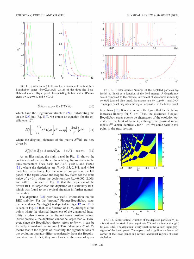
As an illustration, the right panel in Fig. 11 shows thecoefficients of the first three Floquet-Bogoliubov states in thequasimomentum Fock basis for L=3, g=0.1, and F=0.4�31�, where the depletions are ND=0.113, 2.341, and 4.568particles, respectively. For the sake of comparison, the leftpanel in the figure shows the Bogoliubov states for the samevalue of g=0.1, where the depletions are ND=0.002, 2.006,and 4.010. It is seen in Fig. 11 that the depletion of thedriven BEC is larger than the depletion of a stationary BECwhich was found to be a typical situation in further numeri-cal studies.

The depletion �28� provides useful information on theBEC stability. For the “ground” Floquet-Bogoliubov state,the dependence ND=ND�F� is depicted in Figs. 12 and 13. Itis seen in Fig. 12 that, as a function of F, ND diverges at thepoints where the classical increment of the dynamical insta-bility � �also shown in the figure� takes positive values.�More precisely, the depletion cannot be larger than N. How-ever, since the Bogoliubov theory refers to N=�, it can beformally considered as infinite.� This “divergence” of NDmeans that in the regions of instability, the eigenfunctions ofthe evolution operator differ considerably from the Bogoliu-bov structure. In fact, they are chaotic in the sense of quan-

tum chaos �13�. It is also seen in the figure that the depletionincreases linearly for F→�. Thus, the discussed Floquet-Bogoliubov states cannot be eigenstates of the evolution op-erator in the limit of large F, although the classical incre-ments ��k� vanish identically for F→�. We come back to thispoint in the next section.

0 5 100

0.2

0.4

0.6

0.8

1

n

|cn|

0 5 100

0.2

0.4

0.6

0.8

1

n

FIG. 11. �Color online� Left panel: coefficients of the first threeBogoliubov states ���=�ncn�n ,N−2n ,n� of the three-site Bose-Hubbard model. Right panel: Floquet-Bogoliubov states. �Param-eters: J=1, g=0.1, and F=0.4.�

10−1

100

101

0

0.5

1

1.5

2

F

0.05 0.1 0.2 0.40

0.5

1

1.5

2

FIG. 12. �Color online� Number of the depleted particles ND

�solid red lines� as a function of the field strength F �logarithmicscale� compared to the classical increment of dynamical instability�=��F� �dashed blue lines�. Parameters are J=1, g=0.1, and L=3.The upper panel magnifies the region of small F in the lower panel.

F/J

g/J

0.1 0.2 0.3 0.4 0.5

0.1

0.2

0.3

0.4

0.5

0

1

2

3

4

5

6

7

F/J

g/J

0.1 2 4 6 8 100

2

4

6

8

10

0

1

2

3

4

5

(b)

(a)

FIG. 13. �Color online� Number of the depleted particles ND asa function of the static force magnitude F /J and the interaction g /Jfor L=3 sites. The depletion is very small in the yellow �light gray�region of the lower panel. The upper panel magnifies the lower leftcorner of the lower panel and reveals additional regions of smalldepletion.

KOLOVSKY, KORSCH, AND GRAEFE PHYSICAL REVIEW A 80, 023617 �2009�

023617-8

The intervals of small depletion observed in Fig. 12 de-pend, of course, also on the interaction g. The full parameterdependence of the depletion �28� is shown in Fig. 13. Forrelatively low values of g /J and F /J �upper panel�, we find ahighly organized web of stability regions, whereas the be-havior for larger parameters �lower panel� shows a simplerstructure. These many-particle results can be directly com-pared to the mean-field stability diagrams in Fig. 1 whichconfirms the relationship between BEC depletion and mean-field stability.

For the sake of completeness, we also briefly discuss thecorresponding quasienergies E �see Eq. �30�� which are de-fined modulo � times the Bloch frequency, i.e., E�,j =E�,0+ jF, j=0, �1, . . .. The lower panel of Fig. 14 displays thequasienergies of the five Floquet-Bogoliubov states withsmallest ND. The system parameters are J=1, g=0.1, and L=3 as in Fig. 12. For clarity, three Floquet zones are shownin the figure. As expected, the spectrum is equidistant with alevel spacing correlated with the depletion. Note the apparentirregularity in the windows around F=0.2 and F=0.17,which is related to the region of dynamical instability of themean-field system. For comparison, the upper panel showsthe number of depleted particles ND as in Fig. 12 with alinearly scaled F axis. In the regions of finite depletion, themost stable quasienergy states appear to be very sensitiveagainst a variation of F.

B. Bloch oscillations

The microscopic dynamics of BOs was considered earlierin a number of papers summarized in Ref. �13� with focus onthe regime of low filling factors n=N /L�1. In the presentwork, to make a link to the mean-field dynamics, we simu-late BOs for a relatively large filling factor.

We investigate the dynamics in dependence on the force Ffor N=15 and N=20 atoms in a lattice with L=5 sites. Sincethe plots are very similar, only the results with N=15 are

shown. The value of the microscopic interaction constant isset to W=0.1 / n so that the macroscopic interaction constantis g=0.1, and the hopping matrix element J=1. The initialwave function is chosen as the SU�L� coherent state �22�.

In Fig. 15, we show the dynamics of the many-particlecounterpart of the mean-field quantity �16�, that is, the ex-pectation value of the many-particle momentum

p�t� =1

2iN���t���

l

al+1† ale

−iFt − �H.c.����t�� , �33�

for N=15 and the three values of F chosen in different dy-namical regimes as shown in Figs. 6, 8, and 10.

The upper panel of Fig. 15 corresponds to F=0.1, whichfalls into the region of dynamical instability of the mean-field system. Here, the quantum many-particle BO decays invery good agreement with the mean-field ensemble shown inthe upper panel of Fig. 6 �note that finer details are alsoreproduced�. This demonstrates that the ensemble-averagedmean-field dynamics is capable of describing important as-pects of the full many-particle system �24�.

In the middle panel of Fig. 15, we have F=0.4, where thesystem is stable. Here, the quantum many-particle BOs per-sist in time, also agreeing with the ensemble-averaged mean-field dynamics. As discussed above, in this regime, the en-semble average is of little influence, i.e., the state is fullycondensed and can be described by a single mean-field tra-jectory instead.

The third case, F=10, depicted in the lower panel of Fig.15, requires a separate consideration. Indeed, as mentionedin the previous section, in the limit of large F, the Floquet-Bogoliubov states are not eigenstates of the evolution opera-tor �29�. Instead, it can be shown that those are the Fockstates �n� �13�. Thus the time evolution of the wave functionis given by

0.1 0.2 0.3 0.4

−0.5

0

0.5

F

E

0.1 0.2 0.3 0.40

1

2D

FIG. 14. �Color online� Lower panel: quasienergy spectrum ofthe Floquet-Bogoliubov states as a function of the field strength F�same parameters as in Fig. 12�. Upper panel: number of the de-pleted particles ND.

−1

0

1

−1

0

1

0 20 40 60 80 100 120−1

0

1

t/TJ

p(t)

FIG. 15. �Color online� Bloch oscillations of N=15 atoms in alattice with L=5 sites for J=1, W=0.1 /3, and F=0.1 �top�, F=0.4 �middle�, and F=10 �bottom�. Shown is the many-particlemean momentum p�t� given in Eq. �33�.

BLOCH OSCILLATIONS OF BOSE-EINSTEIN… PHYSICAL REVIEW A 80, 023617 �2009�

023617-9

���t�� = �n

cn exp− iWt

2 �l=1

L

nl�nl − 1���n� . �34�

Equation �34� implies a periodic recovering of the initialstate �22� at times which are multiples of TW=2� /W and,hence, periodic revivals of BOs �28�. It should be stressedthat these revivals are a pure quantum many-particle effectdue to the finiteness of W and n. This constructive interfer-ence cannot be explained within the ensemble-averagedmean-field approach. However, the breakdown can be de-scribed by the ensemble averaging and is due to dephasing,as explained in Sec. II B.

IV. SUMMARY

We have studied an N-particle system, a Bose-HubbardHamiltonian with linearly increasing on-site energies. Thissystem can be conveniently reduced to a finite lattice with Lsites by using gauge transformation and imposing periodicboundary conditions.

Such a model can be used to describe important featuresof realistic systems, as for instance the dynamics of coldatoms or BECs in an optical lattice under the influence of thegravitational field �1–12�, or many-particle systems in ring-shaped optical lattices as proposed in �32� with additionaldriving. It should be noted, however, that it neglects a num-ber of features. The space dimension is reduced to a quasi-one-dimensional setting, a decay of the system via Zenertransitions to higher bands is excluded, the lattice is dis-cretized and truncated, and the interaction is simplified. Nev-ertheless, this model has been found to describe experimentalresults quite well. Further, the Bose-Hubbard model is ofinterest in its own right, as evident from the large number ofstudies exploring its properties which are remarkably rich.

In the present paper, we have studied the Bose-Hubbardmodel for relatively small number of lattice sites L�5 butrelatively large number of particles up to N=20 to make alink with the mean-field dynamics. Our aim was twofold.First, we have demonstrated how the modulation instabilityobserved in the mean-field system is manifested in the many-particle case. We have shown that a reasonable measure ofthe N-particle instability is provided by the quantity �28�.Second, we have explored the possibility to describe the timeevolution of many-particle expectation values in terms ofmean-field trajectories, averaged over an ensemble con-structed from the SU�L� phase-space distribution of the ini-tial many-particle state. We found that this �averaged� mean-field dynamics agrees remarkably well with the full quantummany-particle behavior in a number of cases. The only ex-ception was the presence of many-particle revivals for strongfields which is a pure quantum phenomenon.

These observations suggest an application of the mean-field ensemble method to investigate the properties for largerlattices and larger particle numbers where many-particlecomputations are much more difficult or virtually impos-sible. Furthermore, it will be of interest to study the interre-lation between classical chaotic motion and stable or decay-ing Bloch oscillations for more lattice sites where one canpossibly make contact with recent related studies of the

force-free, F=0, case both for the mean-field �33,34� and themany-particle descriptions �30,35�.

ACKNOWLEDGMENTS

We thank D. Witthaut and F. Trimborn for valuable com-ments. Support from the Deutsche Forschungsgemeinschaftvia the Graduiertenkolleg “Nichtlineare Optik und Ultra-kurzzeitphysik” is gratefully acknowledged.

APPENDIX A: STABILITY MATRIX

It is instructive to consider the DNLSE �6� from the view-point of the general theory of nonlinear dynamics. Then thesolution with the initial condition al�t=0�=1,

al�t� = expiJ

Fsin�Ft�� , �A1�

is nothing other than a periodic trajectory in a2L-dimensional phase space. Thus one may address the ques-tion of stability of this periodic trajectory.

Denoting by a= �a1 , . . . ,aL ,a1� , . . . ,aL

��T the devia-tion from an arbitrary trajectory a�t� and linearizing theDNLSE around this trajectory, we have

id

dta = M�a�t��a , �A2�

where M�a�t�� is a 2L�2L matrix of the following structure:

M�a�t�� = A + gB gC

− gC� − �A + gB�� � , �A3�

Al,m = −J

2�l+1,meiFt + l−1,me−iFt� , �A4�

Bl,m = �al�t��2l,m, Cl,m = al2�t�l,m. �A5�

Inserting the trajectory �A1� into Eq. �A2�, the linear equa-

tion �A2� takes a form where the matrix M�t� is periodic intime. Finally, we introduce the stroboscopic map for the dis-crete time tn=TBn,

a�tn+1� = Ua�tn�, U = exp�− i 0

TB

M�t�dt� . �A6�

This stability matrix U is symplectic and hence the consid-ered periodic trajectory �A1� is stable if and only if all itseigenvalues lie on the unit circle.

Using the unitary transformation U→VUV−1, where

V = T 0

0 T�, Tl,m = L−1/2 exp i2�k

Ll� , �A7�

the stability matrix U can be factorized into L decoupled 2�2 matrices which can be labeled as U�k� with k=0, �1, . . . , � �L−1� /2. The matrix U�0� is not of interest

KOLOVSKY, KORSCH, AND GRAEFE PHYSICAL REVIEW A 80, 023617 �2009�

023617-10

here because its eigenvalues are always located on the unitcircle. The explicit form of the matrix U��k� is given by Eq.�13� and, depending on F, its eigenvalues 1,2 either lie onthe unit circle �with 2=1

�� or on the real axis �with 2

=1 /1�. We have stability in the first case and instability inthe second case.

APPENDIX B: MEAN-FIELD ENSEMBLE

Let us recall that the mean-field dynamics of the site am-plitudes al �or, alternatively, the quasimomentum amplitudesbk� appears as a canonical Hamiltonian evolution in a2L-dimensional complex phase space which conserves thenorm, i.e., the phase space is the surface of a complexsphere. In order to approximate the many-particle dynamics,we construct an ensemble of mean-field trajectoriesrepresenting the initial many-body state ���0��. This isachieved most conveniently by using the quantum Husimiphase-space distribution �24�, the projection onto SU�L� co-herent states which in the quasimomentum representation isgiven by

�b�q =1

N! �

k=−�L−1�/2

�L−1�/2

bkbk†�N

�0� , �B1�

with b= �b−�L−1�/2 , . . . ,b0 , . . . ,b�L−1�/2� and �k�bk�2=L. For theinitial many-particle state �22�, this Husimi density Q�b�= ��b ���0���2 is easily calculated as

Q�b� = B�b0�2N, �B2�

where B is a normalization constant. Note that the probabil-ity density for the vector components depends only on thezero-mode probability �b0�2 and is strongly localized in theregion close to its maximum value �b0�2=L for large particlenumber N.

Numerically, one can construct the ensemble �B2� bymeans of a rejection method �36�. First, one generates Lrandomly distributed real numbers rk in the unit interval withrandom phases �k and normalizes the random vector withcomponents zk=rke

i�k to unity. Another random number v inthe unit interval is chosen in order to decide if the generatedvector is accepted as a part of the ensemble: it is accepted ifv� �z0�2N and rejected otherwise. Finally, we renormalize asbk=Lzk. If desired, the ensemble can be Fourier trans-formed to yield the corresponding ensemble of lattice siteamplitudes al.

�1� M. Ben Dahan, E. Peik, J. Reichel, Y. Castin, and C. Salomon,Phys. Rev. Lett. 76, 4508 �1996�.

�2� M. G. Raizen, C. Salomon, and Q. Niu, Phys. Today 50�7��1997� 30.

�3� B. P. Anderson and M. A. Kasevich, Science 282, 1686�1998�.

�4� O. Morsch, J. H. Müller, M. Cristiani, D. Ciampini, and E.Arimondo, Phys. Rev. Lett. 87, 140402 �2001�.

�5� M. Cristiani, O. Morsch, J. H. Müller, D. Ciampini, and E.Arimondo, Phys. Rev. A 65, 063612 �2002�.

�6� M. Jona-Lasinio, O. Morsch, M. Cristiani, N. Malossi, J. H.Müller, E. Courtade, M. Anderlini, and E. Arimondo, Phys.Rev. Lett. 91, 230406 �2003�.

�7� H. Ott, E. de Mirandes, F. Ferlaino, G. Roati, G. Modugno, andM. Inguscio, Phys. Rev. Lett. 92, 160601 �2004�.

�8� D. Witthaut, M. Werder, S. Mossmann, and H. J. Korsch, Phys.Rev. E 71, 036625 �2005�.

�9� S. Wimberger, R. Mannella, O. Morsch, E. Arimondo, A. R.Kolovsky, and A. Buchleitner, Phys. Rev. A 72, 063610�2005�.

�10� C. Sias, A. Zenesini, H. Lignier, S. Wimberger, D. Ciampini,O. Morsch, and E. Arimondo, Phys. Rev. Lett. 98, 120403�2007�.

�11� M. Gustavsson, E. Haller, M. J. Mark, J. G. Danzl, G. Rojas-Kopeinig, and H.-C. Nägerl, Phys. Rev. Lett. 100, 080404�2008�.

�12� M. Fattori, C. D’Errico, G. Roati, M. Zaccanti, M. Jona-Lasinio, M. Modugno, M. Inguscio, and G. Modugno, Phys.Rev. Lett. 100, 080405 �2008�.

�13� A. R. Kolovsky and H. J. Korsch, Int. J. Mod. Phys. B 18,1235 �2004�.

�14� A. Smerzi and A. Trombettoni, Phys. Rev. A 68, 023613�2003�.

�15� M. Holthaus and S. Stenholm, Eur. Phys. J. B 20, 451 �2001�.�16� S. Mossmann and C. Jung, Phys. Rev. A 74, 033601 �2006�.�17� B. Wu and J. Liu, Phys. Rev. Lett. 96, 020405 �2006�.�18� E. M. Graefe and H. J. Korsch, Phys. Rev. A 76, 032116

�2007�.�19� X. Luo, Q. Xie, and B. Wu, Phys. Rev. A 77, 053601 �2008�.�20� M. P. Strzys, E. M. Graefe, and H. J. Korsch, New J. Phys. 10,

013024 �2008�.�21� C. Weiss and N. Teichmann, Phys. Rev. Lett. 100, 140408

�2008�.�22� A. R. Kolovsky, e-print arXiv:cond-mat/0412195.�23� Y. Zheng, M. Kostrun, and J. Javanainen, Phys. Rev. Lett. 93,

230401 �2004�.�24� F. Trimborn, D. Witthaut, and H. J. Korsch, Phys. Rev. A 77,

043631 �2008�.�25� A. R. Kolovsky, E. A. Gómez, and H. J. Korsch, e-print

arXiv:0904.4549.�26� G. B. Berman and A. R. Kolovsky, Sov. Phys. JETP 50, 1116

�1984�.�27� See the special issue of Chaos �2005�, Focus issue 15, devoted

to 50th anniversary of the Fermi-Pasta-Ulam problem.�28� A. R. Kolovsky, Phys. Rev. Lett. 90, 213002 �2003�.�29� A. J. Leggett, Rev. Mod. Phys. 73, 307 �2001�.�30� A. R. Kolovsky, New J. Phys. 8, 197 �2006�; Phys. Rev. Lett.

99, 020401 �2007�.�31� In the numerical computations discussed in the following, we

used in most cases N=100 particles. The results are stablewhen N is increased keeping the value of WN constant unlessexplicitly stated.

BLOCH OSCILLATIONS OF BOSE-EINSTEIN… PHYSICAL REVIEW A 80, 023617 �2009�

023617-11

�32� L. Amico, A. Osterloh, and F. Cataliotti, Phys. Rev. Lett. 95,063201 �2005�.

�33� P. Villain and M. Lewenstein, Phys. Rev. A 62, 043601 �2000�.�34� A. C. Cassidy, D. Mason, V. Dunjko, and M. Olshanii, e-print

arXiv:0805.3388 �2008�.

�35� G. P. Berman, F. Borgonovi, F. M. Izrailev, and A. Smerzi,Phys. Rev. Lett. 92, 030404 �2004�.

�36� W. H. Press, S. A. Teukolsky, W. T. Vetterling, and B. P. Flan-nery, Numerical Recipes, 3rd ed. �Cambridge University Press,London, 2007�.

KOLOVSKY, KORSCH, AND GRAEFE PHYSICAL REVIEW A 80, 023617 �2009�

023617-12