blind and semi-blind channel order estimation in simo...

BLIND AND SEMI-BLIND CHANNEL ORDER ESTIMATION IN SIMO SYSTEMS

A THESIS SUBMITTED TOTHE GRADUATE SCHOOL OF NATURAL AND APPLIED SCIENCES

OFMIDDLE EAST TECHNICAL UNIVERSITY

BY

SERKAN KARAKUTUK

IN PARTIAL FULFILLMENT OF THE REQUIREMENTSFOR

THE DEGREE OF DOCTOR OF PHILOSOPHYIN

ELECTRICAL AND ELECTRONICS ENGINEERING

SEPTEMBER 2009

Approval of the thesis:


submitted by SERKAN KARAKUTUK in partial fulfillment of the requirements for the de-gree ofDoctor of Philosophy in Electrical and Electronics Engineering Department, MiddleEast Technical University by,

Prof. Dr. Canan OzgenDean, Graduate School of Natural and Applied Sciences

Prof. Dr. Ismet ErkmenHead of Department, Electrical and Electronics Engineering

Prof. Dr. T. Engin TuncerSupervisor, Electrical and Electronics Engineering Department,METU

Examining Committee Members:

Prof. Dr. T. Engin TuncerElectrical and Electronics , METU

Prof. Dr. Kerim DemirbasElectrical and Electronics , METU

Assoc. Prof. Dr. Elif Uysal BıyıkogluElectrical and Electronics , METU

Assist. Prof. Dr. Cagatay CandanElectrical and Electronics , METU

Assist. Prof. Dr. Yakup OzkazancElectrical and Electronics , Hacettepe University

Date:

I hereby declare that all information in this document has been obtained and presentedin accordance with academic rules and ethical conduct. I also declare that, as requiredby these rules and conduct, I have fully cited and referenced all material and results thatare not original to this work.

Name, Last Name: SERKAN KARAKUTUK

Signature :

iii

ABSTRACT


Karakutuk, Serkan

Ph.D, Department of Electrical and Electronics Engineering

Supervisor : Prof. Dr. T. Engin Tuncer

September 2009, 138 pages

Channel order estimation is an important problem in many fields including signal processing,

communications, acoustics, and more. In this thesis, blind channel order estimation problem

is considered for single-input, multi-output (SIMO) FIR systems. The problem is to estimate

the effective channel order for the SIMO system given only the output samples corrupted by

noise. Two new methods for channel order estimation are presented. These methods have

several useful features compared to the currently known techniques. They are guaranteed to

find the true channel order for noise free case and they perform significantly better for noisy

observations. These algorithms show a consistent performance when the number of observa-

tions, channels and channel order are changed. The proposed algorithms are integrated with

the least squares smoothing (LSS) algorithm for blind identification of the channel coeffi-

cients. LSS algorithm is selected since it is a deterministic algorithm and has some additional

features suitable for order estimation. The proposed algorithms are compared with a variety

of different algorithms including linear prediction (LP) based methods. LP approaches are

known to be robust to channel order overestimation. In this thesis, it is shown that significant

gain can be obtained compared to LP based approaches when the proposed techniques are

used. The proposed algorithms are also compared with the oversampled single-input, single-

iv

output (SISO) system with a generic decision feedback equalizer, and better mean-square

error performance is observed for the blind setting.

Channel order estimation problem is also investigated for semi-blind systems where a pilot

signal is used which is known at the receiver. In this case, two new methods are proposed

which exploit the pilot signal in different ways. When both unknown and pilot symbols are

used, a better estimation performance can be achieved compared to the proposed blind meth-

ods. The semi-blind approach is especially effective in terms of bit error rate (BER) evaluation

thanks to the use of pilot symbols in better estimation of channel coefficients. This approach

is also more robust to ill-conditioned channels. The constraints for these approaches, such

as synchronization, and the decrease in throughput still make the blind approaches a good

alternative for channel order estimation. True and effective channel order estimation topics

are discussed in detail and several simulations are done in order to show the significant per-

formance gain achieved by the proposed methods.

Keywords: channel order estimation, channel identification, channel equalization

v

OZ

SIMO SISTEMLERDE GOZU KAPALI VE YARI KAPALI KANAL DERECESIKESTIRIMI

Karakutuk, Serkan

Doktora, Elektrik Elektronik Muhendislig Bolumu

Tez Yoneticisi : Prof. Dr. T. Engin Tuncer

Eylul 2009, 138 sayfa

Kanal derecesi kestirimi sinyal isleme, haberlesme, akustik ve benzeri alanlar icin onemli

bir problemdir. Bu tezde, gozu kapalı kanal derecesi kestirimi problemi tek girisli cok cıktılı

(SIMO) FIR sistemler icin incelenmistir. Problem, sadece gurultulu SIMO sistemi cıktılarının

kullanılarak etkin kanal derecesinin kestirilmesidir. Kanal derecesi kestirimi icin iki yontem

onerilmistir. Onerilen yontemlerin bilinen yontemlere nazaran bir cok yararlı ozelligi bulun-

maktadır. Onerilen yontemler gurultusuz ortamda dogru kanal derecesi kestirimini garanti

etmekte ve gurultulu ortamda da kayda deger sekilde daha iyi basarım gostermektedir. Bu

algoritmalar kanal derecesi, kanal sayısı ve veri boyunun degisimine karsı tutarlı bir davranıs

gostermektedir. Onerilen algoritmalar, kanal katsayılarının gozu kapalı kestirimine yonelik

olarak en kucuk kareler yumusatma (LSS) algoritması ile entegre sekilde calısmaktadır. LSS

algoritmasının secilmesinin nedeni belirlenimci bir yontem olması ve kanal derecesi kestirimi

icin uygun bazı ek ozelliklerinin bulunmasıdır. Onerilen algoritmalar, dogrusal tahmin (LP)

yontemlerinin de yer aldıgı degisik bir cok algoritma ile karsılastırılmıstır. LP yaklasımları

kanal derecesinin ustten kestirimine karsı direnclidir. Bu tezde, onerilen yontemler kul-

lanıldıgında, LP tabanlı yontemlere nazaran onemli oranda kazanc saglanabilecegi gosteril-

vi

mistir. Onerilen yontemler, yuksek hızda orneklenmis SISO sistemler icin DFE yontemi ile

de karsılastırılmıs ve gozu kapalı durumda daha iyi hata kareleri ortalaması performansı elde

edildigi gorulmustur.

Kanal derecesi kestirimi problemi, pilot sembollerin kullanıldıgı sistemler icin de incelenmistir.

Bunun icin, pilot sembollerini farlı sekilde kullanan gozu yarı-kapalı kanal derecesi kestirimi

algoritmaları onerilmistir. Bilinen ve bilinmeyen semboller birlikte kullanıldıgı zaman, gozu

kapalı yontemlere nazaran daha iyi kestirim performansı saglanabilmektedir. Kanal kestirimi

dogrulugu pilot sembollerin kullanımı ile arttıgı icin, gozu yarı-kapalı yaklasım ile ozellikle

bit hata oranı (BER) acısından daha iyi basarım elde edilebilmektedir. Bu yaklasımın diger bir

ozelligi ise kotu durumlu (ill-conditioned) kanallara karsı daha direncli olmasıdır. Ote yan-

dan, eszamanlama ve veri akısındaki dusus gibi problemler nedeniyle gozu kapalı yontemler

hala kanal derecesi icin iyi bir alternatif olarak gozukmektedir. Dogru ve etkin kanal dere-

cesi kestirimi konuları ayrıntılı sekilde tartısılmıs ve onerilen yontemler ile elde edilen kayda

deger basarım kazancını gostermek icin cesitli benzetimler yapılmıstır.

Anahtar Kelimeler: kanal derecesi kestirimi, kanal tanımlama, kanal esitleme

vii

To my love Gulay and my parents.

viii

ACKNOWLEDGMENTS

It is a pleasure for me to express my sincere gratitude to my supervisor Prof. Dr. T. Engin

Tuncer for his guidance, advice, sensitivity, encouragements and sharing all his thoughts.

I also want to thank to my colleagues in MIKES for their support. Moreover, I am thankful to

my company MIKES for letting and supporting my thesis.

I would like to thank to METU Sensor Array and Multichannel Signal Processing Group for

their useful comments and support during my thesis work.

I would also like to thank for the scholarship received from the Scientific and Technological

Research Council of Turkey (TUBITAK).

I will also never forget to unending reliance, love and support of my family all the times.

Finally, I want to thank my love, Gulay Tuncer, who is always by my side and helped me to

keep myself away from hopelessness.

ix

TABLE OF CONTENTS

ABSTRACT . . . . . . . . . . . . . . . . . . . . . . . . . . . . . . . . . . . . . . . . iv

OZ . . . . . . . . . . . . . . . . . . . . . . . . . . . . . . . . . . . . . . . . . . . . . vi

DEDICATION . . . . . . . . . . . . . . . . . . . . . . . . . . . . . . . . . . . . . . viii

ACKNOWLEDGMENTS . . . . . . . . . . . . . . . . . . . . . . . . . . . . . . . . . ix

TABLE OF CONTENTS . . . . . . . . . . . . . . . . . . . . . . . . . . . . . . . . . x

LIST OF TABLES . . . . . . . . . . . . . . . . . . . . . . . . . . . . . . . . . . . . xiv

LIST OF FIGURES . . . . . . . . . . . . . . . . . . . . . . . . . . . . . . . . . . . . xv

CHAPTERS

1 INTRODUCTION . . . . . . . . . . . . . . . . . . . . . . . . . . . . . . . 1

1.1 Motivation and Objectives . . . . . . . . . . . . . . . . . . . . . . . 1

1.2 Previous Works . . . . . . . . . . . . . . . . . . . . . . . . . . . . 4

1.3 Contributions . . . . . . . . . . . . . . . . . . . . . . . . . . . . . 6

1.4 Organization of the Thesis . . . . . . . . . . . . . . . . . . . . . . . 7

2 BLIND SYSTEM IDENTIFICATION . . . . . . . . . . . . . . . . . . . . . 8

2.1 Introduction . . . . . . . . . . . . . . . . . . . . . . . . . . . . . . 8

2.2 System Model . . . . . . . . . . . . . . . . . . . . . . . . . . . . . 10

2.3 Channel Identifiability . . . . . . . . . . . . . . . . . . . . . . . . . 13

2.4 Subspace Method . . . . . . . . . . . . . . . . . . . . . . . . . . . 14

2.5 Least Squares Smoothing Method . . . . . . . . . . . . . . . . . . . 16

2.5.1 Assumptions and Properties . . . . . . . . . . . . . . . . 17

2.5.2 Least Squares Smoothing Algorithm . . . . . . . . . . . . 18

2.5.2.1 Channel Identification from Input Subspace . 19

2.5.2.2 Channel Identification from Output Subspace 20

x

2.5.3 General Formulation of LSS . . . . . . . . . . . . . . . . 22

2.5.4 Joint Order Detection and Channel Estimation by UsingLSS (LSS) [3] . . . . . . . . . . . . . . . . . . . . . . . . 24

2.5.5 Algorithm: . . . . . . . . . . . . . . . . . . . . . . . . . 25

2.6 Linear Prediction Method . . . . . . . . . . . . . . . . . . . . . . . 26

2.7 Channel Order Estimation . . . . . . . . . . . . . . . . . . . . . . . 29

2.7.1 Akaiki Information Criteria (AIC) [20] . . . . . . . . . . 31

2.7.2 Minimum Description Length (MDL) [19] . . . . . . . . . 32

2.7.3 Liavas Algorithm [4] . . . . . . . . . . . . . . . . . . . . 32

2.7.4 ID+EQ Algorithm [24] . . . . . . . . . . . . . . . . . . . 33

2.7.4.1 Identification Part . . . . . . . . . . . . . . . 33

2.7.4.2 Equalization Part . . . . . . . . . . . . . . . 35

2.7.4.3 Combined Cost Function . . . . . . . . . . . 37

3 BLIND CHANNEL ORDER ESTIMATION . . . . . . . . . . . . . . . . . 38

3.1 Introduction . . . . . . . . . . . . . . . . . . . . . . . . . . . . . . 38

3.2 System Model and Problem Definition . . . . . . . . . . . . . . . . 40

3.3 Channel Output Error (COE) Algorithm . . . . . . . . . . . . . . . 42

3.3.1 Blind Channel Estimation . . . . . . . . . . . . . . . . . 43

3.3.2 Channel Equalization and Input Estimation . . . . . . . . 47

3.3.3 Data Unstacking . . . . . . . . . . . . . . . . . . . . . . 47

3.3.4 Channel Output Error . . . . . . . . . . . . . . . . . . . . 48

3.4 Channel Matrix Recursion Algorithm (CMR) Algorithm . . . . . . . 49

3.5 Evaluation and Comparison of the COE and CMR Algorithms . . . . 52

3.6 Conclusion . . . . . . . . . . . . . . . . . . . . . . . . . . . . . . . 54

4 CHANNEL ORDER ESTIMATION USING TRAINING DATA . . . . . . . 58

4.1 Introduction . . . . . . . . . . . . . . . . . . . . . . . . . . . . . . 58

4.2 Training Based Channel Estimation . . . . . . . . . . . . . . . . . . 60

4.3 Channel Order Estimation Using Blind Channel Estimator and Train-ing Data, CIEB . . . . . . . . . . . . . . . . . . . . . . . . . . . . . 65

4.3.1 Channel Estimation . . . . . . . . . . . . . . . . . . . . . 66

4.3.2 Channel Equalization . . . . . . . . . . . . . . . . . . . . 67

xi

4.3.3 Data Unstacking . . . . . . . . . . . . . . . . . . . . . . 68

4.3.4 Synchronization . . . . . . . . . . . . . . . . . . . . . . . 68

4.3.5 CIEB Cost Function . . . . . . . . . . . . . . . . . . . . 69

4.4 Channel Order Estimation Using Semi-blind Channel Estimator andTraining Data, (CIES) . . . . . . . . . . . . . . . . . . . . . . . . . 69

4.4.1 Semi-blind Channel Estimation . . . . . . . . . . . . . . 70

4.4.2 CIES Cost Function . . . . . . . . . . . . . . . . . . . . . 72

4.4.3 Simulations . . . . . . . . . . . . . . . . . . . . . . . . . 72

4.5 Conclusion . . . . . . . . . . . . . . . . . . . . . . . . . . . . . . . 76

5 EFFECTIVE CHANNEL ORDER ESTIMATION . . . . . . . . . . . . . . . 78

5.1 Introduction . . . . . . . . . . . . . . . . . . . . . . . . . . . . . . 78

5.2 Effective Channel Order . . . . . . . . . . . . . . . . . . . . . . . . 81

5.3 Evaluation of The Performance of Channel Order Estimation Algo-rithms in Estimating The Effective Channel Order . . . . . . . . . . 84

5.3.1 Fixed Channel . . . . . . . . . . . . . . . . . . . . . . . . 84

5.3.2 Random Channel . . . . . . . . . . . . . . . . . . . . . . 92

5.4 BER When Different Channel Estimation Algorithms are Used . . . 98

5.4.1 Performance of The Channel Estimation Algorithms in Caseof Channel Order Mismatch . . . . . . . . . . . . . . . . 98

5.4.2 Performance of Channel Estimators, MLP and LSS, withDifferent Channel Order Estimation Algorithms . . . . . . 103

5.5 Performance Comparison of Proposed Methods with DFE in Frac-tionally Spaced SISO Channels . . . . . . . . . . . . . . . . . . . . 110

5.6 Conclusion . . . . . . . . . . . . . . . . . . . . . . . . . . . . . . . 113

6 CONCLUSION . . . . . . . . . . . . . . . . . . . . . . . . . . . . . . . . . 115

REFERENCES . . . . . . . . . . . . . . . . . . . . . . . . . . . . . . . . . . . . . . 120

APPENDICES

A PROOFS . . . . . . . . . . . . . . . . . . . . . . . . . . . . . . . . . . . . 124

A.1 Reorganized Convolution Equation . . . . . . . . . . . . . . . . . . 124

A.2 Lemma 1 . . . . . . . . . . . . . . . . . . . . . . . . . . . . . . . . 126

A.3 Lemma 2 . . . . . . . . . . . . . . . . . . . . . . . . . . . . . . . . 127

A.4 Lemma-3 . . . . . . . . . . . . . . . . . . . . . . . . . . . . . . . . 128

xii

A.5 Theorem 1 . . . . . . . . . . . . . . . . . . . . . . . . . . . . . . . 130

A.5.1 Correct Channel Order Estimation . . . . . . . . . . . . . 130

A.5.2 Overestimated Channel Order . . . . . . . . . . . . . . . 131

A.5.3 Underestimated Channel Order . . . . . . . . . . . . . . . 134

A.6 Theorem-2 . . . . . . . . . . . . . . . . . . . . . . . . . . . . . . . 134

A.6.1 Correct Channel Order Estimation . . . . . . . . . . . . . 135

A.6.2 Overestimated Channel Order . . . . . . . . . . . . . . . 135

A.6.3 Underestimated Channel Order . . . . . . . . . . . . . . . 137

CURRICULUM VITAE . . . . . . . . . . . . . . . . . . . . . . . . . . . . . . . . . 138

xiii

LIST OF TABLES

TABLES

Table 3.1 AIC, Liavas and MDL performances (percentage of true channel order es-

timate) for different channel order and number of channels. S NR = 15dB, input

length = 100. . . . . . . . . . . . . . . . . . . . . . . . . . . . . . . . . . . . . . 55

Table 3.2 COE and CMR performances (percentage of true channel order estimate)

for different channel order and number of channels. S NR = 15dB, input length

= 100. . . . . . . . . . . . . . . . . . . . . . . . . . . . . . . . . . . . . . . . . 55

Table 4.1 BER performance of training based method against estimated channel order

and different code lengths. True channel order is L = 4 and S NR = 10dB. . . . . 63

Table 5.1 Channel coefficients of the channel given in [15], L=5, P=4. . . . . . . . . 99

xiv

LIST OF FIGURES

FIGURES

Figure 1.1 Channel impulse response showing the significant part and tail of the chan-

nels. Tail coefficients are uniformly distributed between −γ/2 and + γ/2. . . . . . 2

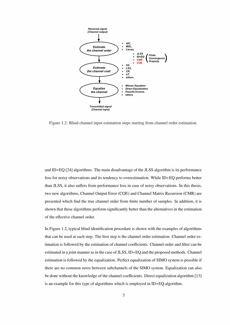
Figure 1.2 Blind channel input estimation steps starting from channel order estimation. 5

Figure 2.1 SIMO Channel Model . . . . . . . . . . . . . . . . . . . . . . . . . . . . 11

Figure 2.2 Projection of output data onto projection subspace Z . . . . . . . . . . . . 19

Figure 2.3 isomorphism between input and output subspaces . . . . . . . . . . . . . . 21

Figure 2.4 Isomorphism between input and output subspaces for l , L (a) l < L (b) l > L 23

Figure 2.5 Linear prediction algorithm. Zero forcing equalization. . . . . . . . . . . . 28

Figure 2.6 CR blind channel identification for SIMO channel. . . . . . . . . . . . . . 34

Figure 3.1 Channel output estimation for channel order L in COE algorithm. . . . . . 43

Figure 3.2 Estimated SIMO channel with common channel zeros. . . . . . . . . . . . 44

Figure 3.3 Pole-zero plots for the estimated channels by SS and LSS algorithms. At

each row of the figure a different channel is used. True channel order L = 3 and

the number of subchannels is P = 2. o and + indicates the zeros of the first and

second subchannels of the SIMO system. . . . . . . . . . . . . . . . . . . . . . . 46

Figure 3.4 Channel output error (COE) for noisy observations. . . . . . . . . . . . . . 49

Figure 3.5 Overestimated channel order results common channel zeros in LSS. . . . . 50

Figure 3.6 Cost function, ECMR, for channel matrix recursion (CMR) for noisy obser-

vations. . . . . . . . . . . . . . . . . . . . . . . . . . . . . . . . . . . . . . . . . 52

xv

Figure 3.7 Probability density functions (with shape-preserving curve fitting) of the

channel order estimation algorithms: MDL, AIC, Liavas, JLSS, ID+EQ and pro-

posed methods COE and CMR. S NR = 15dB, the true channel order is L = 5 and

P = 3. . . . . . . . . . . . . . . . . . . . . . . . . . . . . . . . . . . . . . . . . 55

Figure 3.8 Channel order estimation performance for L = 3, P = 3 and input length

= 100. . . . . . . . . . . . . . . . . . . . . . . . . . . . . . . . . . . . . . . . . 56


= 100. . . . . . . . . . . . . . . . . . . . . . . . . . . . . . . . . . . . . . . . . 56


= 100. . . . . . . . . . . . . . . . . . . . . . . . . . . . . . . . . . . . . . . . . 57

Figure 4.1 Training sequence is send at start of each frame. T is the length of training

sequence and N is the frame length. . . . . . . . . . . . . . . . . . . . . . . . . . 61

Figure 4.2 BER performance of training based method and CMR method. Channel

order is, L = 4, and it is assumed to be known in training based LS method. . . . 62

Figure 4.3 BER performance of training based method CMR method. Channel order

is overestimated in training based method, L = L + 3. . . . . . . . . . . . . . . . 62

Figure 4.4 Channel order estimation performance when the synchronization is not

achieved. . . . . . . . . . . . . . . . . . . . . . . . . . . . . . . . . . . . . . . 64

Figure 4.5 Channel order estimation with CIEB method. . . . . . . . . . . . . . . . . 66

Figure 4.6 Estimated SIMO channel with common channel zeros. . . . . . . . . . . . 67

Figure 4.7 Channel order estimation with CIES method. . . . . . . . . . . . . . . . . 70

Figure 4.8 (a) Probability of correct channel order estimation versus SNR, (b)BER

versus SNR for L = 3, P = 3. . . . . . . . . . . . . . . . . . . . . . . . . . . . . 74


versus SNR for L = 3, P = 5. . . . . . . . . . . . . . . . . . . . . . . . . . . . . 75


versus SNR for L = 5, P = 5. . . . . . . . . . . . . . . . . . . . . . . . . . . . . 76

Figure 5.1 Channel impulse response showing the significant part and tail of the chan-

nels. Tail coefficients are assumed to be distributed uniformly between −γ/2 and

+ γ/2. . . . . . . . . . . . . . . . . . . . . . . . . . . . . . . . . . . . . . . . . 81

xvi

Figure 5.2 Channel impulse response for Channel-1. h1(n) and h2(n) are the impulse

responses of two channel SIMO system (P = 2). . . . . . . . . . . . . . . . . . . 85

Figure 5.3 Channel impulse response for the microwave channel, Channel-2, is shown

for only 60 samples for clarity. The total number of samples for each channel is

115. h1(n) and h2(n) are the impulse responses of two channel SIMO system (P = 2). 85

Figure 5.4 Channel impulse response for the microwave channel, Channel-3, is shown

for only 60 samples for clarity. The total number of samples for each channel is

150. h1(n) and h2(n) are the impulse responses of two channel SIMO system (P = 2). 86

Figure 5.5 Condition measure, σ2Le+1εLe

, versus candidate channel order and BER versus

candidate channel order for (a) Channel-1. (b) Channel-2, and (c) Channel-3. . . 87

Figure 5.6 (a) Probability of correct effective channel order estimation for Channel-1.

Effective channel order is assumed to be one. (b) BER versus channel order for

Channel-1. . . . . . . . . . . . . . . . . . . . . . . . . . . . . . . . . . . . . . . 90


Effective channel order is assumed to be one. (b) BER versus channel order for

Channel-2. . . . . . . . . . . . . . . . . . . . . . . . . . . . . . . . . . . . . . . 91


Effective channel order is assumed to be two. (b) BER versus channel order for

Channel-3. . . . . . . . . . . . . . . . . . . . . . . . . . . . . . . . . . . . . . . 92

Figure 5.9 Channel order estimation performances for γ = 0.05, Le = 3 and P = 3. . . 95

Figure 5.10 Channel order estimation performances for γ = 0.1, Le = 3 and P = 3. . . . 96

Figure 5.11 Channel order estimation performances for γ = 0.2, Le = 3 and P = 3. . . . 97

Figure 5.12 Channel estimation error versus SNR when (a) channel order is correctly

estimated L = L and (b) channel order is over estimated, L = L + 2 . . . . . . . . . 100

Figure 5.13 Channel estimation error versus channel order when S NR = 15dB. . . . . 100

Figure 5.14 Channel impulse responses of four channel SIMO system. . . . . . . . . . 102

Figure 5.15 Channel estimation error versus SNR when (a) channel order is correctly

estimated L = L and (b) channel order is over estimated, L = L + 2 . . . . . . . . . 103

Figure 5.16 Channel estimation error versus channel order when S NR = 15dB. . . . . 103

xvii

Figure 5.17 Channel order estimation performances of different algorithms. (a) Prob-

ability of correct channel order estimation, (b) Probability density functions of

estimated channel orders with different algorithms when S NR = 15dB. PDF is

obtained from the histogram of the estimated channel orders with curve fitting

technique. . . . . . . . . . . . . . . . . . . . . . . . . . . . . . . . . . . . . . . 105

Figure 5.18 BER and NMSE versus SNR when the true channel order is estimated with

different channel order estimation algorithms (a)-(b) LSS and Wiener equalizer are

used to estimate the channel and input signal for MDL, AIC and Liavas. (c)-(d)

MLP is used to estimate the channel and input signal for MDL, AIC and Liavas. . 106

Figure 5.19 BER and NMSE versus SNR when the true channel order is estimated with

different channel order estimation algorithms. MLP is used with Wiener equalizer

in MDL, AIC and Liavas. . . . . . . . . . . . . . . . . . . . . . . . . . . . . . . 106

Figure 5.20 Channel order estimation performances of different algorithms. (a) Prob-

ability of correct channel order estimation, (b) Probability density functions of

estimated channel orders with different algorithms when S NR = 15dB. PDF is

obtained from the histogram of the estimated channel orders with curve fitting

technique. . . . . . . . . . . . . . . . . . . . . . . . . . . . . . . . . . . . . . . 108

Figure 5.21 BER and NMSE versus SNR when the effective channel order is estimated

with different channel order estimation algorithms (a)-(b) LSS and Wiener equal-

izer are used to estimate the channel and input signal for MDL, AIC and Liavas.

(c)-(d) MLP is used to estimate the channel and input signal for MDL, AIC and

Liavas. (e)-(f) MLP is used with Wiener equalizer in MDL, AIC and Liavas. . . . 109

Figure 5.22 MSE and BER performance of COE, CMR and DFE methods. The channel

given in [15] is used without tail coefficients. . . . . . . . . . . . . . . . . . . . . 112

Figure 5.23 MSE and BER performance of COE, CMR and DFE methods. The channel

given in [15] is used with tail coefficients. . . . . . . . . . . . . . . . . . . . . . . 112

Figure 5.24 MSE and BER performance of COE, CMR and DFE methods. Two chan-

nel case considered with a microwave channel given in ”http://spib.rice.edu/spib/microwave.html”

as chan3.mat. . . . . . . . . . . . . . . . . . . . . . . . . . . . . . . . . . . . . . 113

xviii

CHAPTER 1

INTRODUCTION

1.1 Motivation and Objectives

In this thesis, blind channel order estimation problem in linear time invariant (LTI) finite

impulse response (FIR), single-input multiple-output (SIMO) systems is investigated. SIMO

systems are observed when single-input single-output (SISO) system outputs are oversampled

and polyphase representation is used or alternatively when multiple antennas and receivers are

employed [1, 2]. Blind channel order estimation problem is defined as the estimation of the

order of a FIR SIMO systems given the noisy observations.

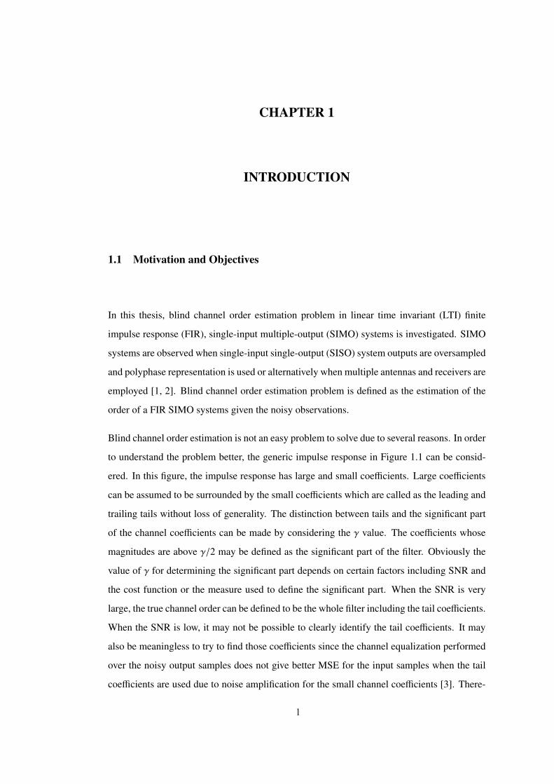
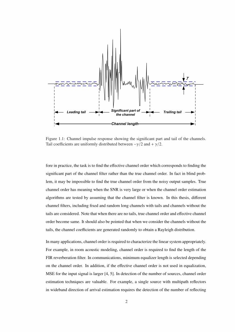
Blind channel order estimation is not an easy problem to solve due to several reasons. In order

to understand the problem better, the generic impulse response in Figure 1.1 can be consid-

ered. In this figure, the impulse response has large and small coefficients. Large coefficients

can be assumed to be surrounded by the small coefficients which are called as the leading and

trailing tails without loss of generality. The distinction between tails and the significant part

of the channel coefficients can be made by considering the γ value. The coefficients whose

magnitudes are above γ/2 may be defined as the significant part of the filter. Obviously the

value of γ for determining the significant part depends on certain factors including SNR and

the cost function or the measure used to define the significant part. When the SNR is very

large, the true channel order can be defined to be the whole filter including the tail coefficients.

When the SNR is low, it may not be possible to clearly identify the tail coefficients. It may

also be meaningless to try to find those coefficients since the channel equalization performed

over the noisy output samples does not give better MSE for the input samples when the tail

coefficients are used due to noise amplification for the small channel coefficients [3]. There-

1

Significant part of

the channelLeading tail Trailing tail

Channel length

Figure 1.1: Channel impulse response showing the significant part and tail of the channels.Tail coefficients are uniformly distributed between −γ/2 and + γ/2.

fore in practice, the task is to find the effective channel order which corresponds to finding the

significant part of the channel filter rather than the true channel order. In fact in blind prob-

lem, it may be impossible to find the true channel order from the noisy output samples. True

channel order has meaning when the SNR is very large or when the channel order estimation

algorithms are tested by assuming that the channel filter is known. In this thesis, different

channel filters, including fixed and random long channels with tails and channels without the

tails are considered. Note that when there are no tails, true channel order and effective channel

order become same. It should also be pointed that when we consider the channels without the

tails, the channel coefficients are generated randomly to obtain a Rayleigh distribution.

In many applications, channel order is required to characterize the linear system appropriately.

For example, in room acoustic modeling, channel order is required to find the length of the

FIR reverberation filter. In communications, minimum equalizer length is selected depending

on the channel order. In addition, if the effective channel order is not used in equalization,

MSE for the input signal is larger [4, 5]. In detection of the number of sources, channel order

estimation techniques are valuable. For example, a single source with multipath reflectors

in wideband direction of arrival estimation requires the detection of the number of reflecting

2

points. Otherwise the DOA algorithms either do not work or report angles with large errors.

Channel order is an important parameter for the blind channel identification problem. In blind

channel identification, the channel order is usually assumed to be known [1, 6, 7, 8, 10, 13] .

In practice, it should be estimated. When the channel order is underestimated, the blind chan-

nel estimation algorithms fail. When the channel order is overestimated, their performance

significantly degrades. Hence, best performance is achieved when the effective channel order

is correctly estimated. Since previous algorithms for channel order estimation are not robust,

this problem has been tried to be solved with linear prediction (LP) based channel estimation

algorithms robust to channel order overestimation [14, 15, 16, 17, 18]. However, LP methods

are based on statistical information of the channel outputs and therefore they require long ob-

servation data to obtain required performance. Furthermore, their performance is not as good

as their deterministic alternatives such as subspace algorithm [6], when the channel order is

known. On the other hand, the main drawback of deterministic algorithms is that their perfor-

mance decreases dramatically when the channel order is not correctly estimated. Therefore

the use of these algorithms is not practical as a consequence of absence of high performance

channel order estimation algorithms. If an accurate and robust channel order estimation algo-

rithm is used with deterministic channel estimator such as proposed in [6, 7, 8] for channel

estimation, a better performance is obtained compared to LP techniques with an algorithm

which has tendency to overestimate.

The main objective of the thesis is to find new blind channel order estimation algorithms for

SIMO systems. The desired properties for a blind channel order estimation algorithms are as

follows:

• It should have finite convergence property. That is channel order can be found correctly

from finite number of sample in noiseless observations. Therefore, fast convergence

can be established for time varying channels and high performance is guaranteed at

high SNR.

• Channel order should also be correctly estimated with high probability at low SNR

ranges. Correct channel order estimation is important to use deterministic channel esti-

mators in an effective manner.

• It should be robust to SIMO channel parameters. That is, it should work properly for

3

different receiver settings (i.e., number of antennas or oversampling rate) and physical

channel parameters (i.e., channel length and channel impulse response).

In this thesis, channel order estimation problem in training based communication system is

also considered. It is targeted to find channel order estimation algorithms, which use training

data to obtain better performance compared to blind methods.

1.2 Previous Works

There are different algorithms for the channel order estimation in the literature. Minimum

Description Length (MDL) [19] and Akaike Information Criteria (AIC) [20] algorithms are

based on the information theoretic criteria. These algorithms require long observations for

accurate extraction of the statistical parameters. It is known that MDL usually performs better

than the AIC and AIC has a tendency for overestimation [4, 21]. Both of these algorithms are

sensitive to colored noise [21] and deviation from idealized Gaussian white noise signal. In

addition, they are very sensitive to SNR variations and data length [22]. Therefore they are

not robust algorithms for practical applications and scenarios.

Joint channel order and channel estimation with LSS method (JLSS) is presented in [3]. It

is shown that JLSS can find the true channel order from finite number of samples in case of

noise free observations. The main disadvantage of the JLSS algorithm is its performance loss

for noisy observations.

Most of the cost functions for order estimation decrease almost monotonically as the channel

order increases, which makes it hard to find the true channel order. This problem is tried to

be overcome by using an empirically chosen penalty coefficient [23]. This penalty term leads

to over or underestimation in many of the information theoretic techniques. In [24], a new

cost function is proposed. This cost function is obtained by combining two cost functions due

to channel identification (ID) and channel equalization (EQ), and hence ID+EQ algorithm

is obtained. The main feature of this cost function is its ”convex - like” shape. Therefore

channel order estimation can be performed by finding the global minimum.

Previously, it is known that there are only two algorithms which are guaranteed to find the

correct channel order from finite number samples in noise free case. These are the JLSS [3]

4

Estimate

the channel order

Estimate

the channel coef.

Equalize

the channel

Received signal

(Channel output)

Transmitted signal

(Channel input)

AIC,

MDL,

Liavas,

SS,

LSS,

CR,

LP,

others

Wiener Equalizer

Direct Equalization

Pseudo-inverse,

others

JLSS

ID+EQ

CMR

COE

Finite

Convergence

Property

Figure 1.2: Blind channel input estimation steps starting from channel order estimation.

and ID+EQ [24] algorithms. The main disadvantage of the JLSS algorithm is its performance

loss for noisy observations and its tendency to overestimation. While ID+EQ performs better

than JLSS, it also suffers from performance loss in case of noisy observations. In this thesis,

two new algorithms, Channel Output Error (COE) and Channel Matrix Recursion (CMR) are

presented which find the true channel order from finite number of samples. In addition, it is

shown that these algorithms perform significantly better than the alternatives in the estimation

of the effective channel order.

In Figure 1.2, typical blind identification procedure is shown with the examples of algorithms

that can be used at each step. The first step is the channel order estimation. Channel order es-

timation is followed by the estimation of channel coefficients. Channel order and filter can be

estimated in a joint manner as in the case of JLSS, ID+EQ and the proposed methods. Channel

estimation is followed by the equalization. Perfect equalization of SIMO system is possible if

there are no common zeros between subchannels of the SIMO system. Equalization can also

be done without the knowledge of the channel coefficients. Direct equalization algorithm [13]

is an example for this type of algorithms which is employed in ID+EQ algorithm.

5

1.3 Contributions

Summary of main the contributions are as follows:

• Blind channel order estimation for SIMO systems is considered. Blind channel order

estimation problem especially the effective channel order estimation problem is covered

in detail. The comparisons and the results in this regard are unique in the literature.

• Two new blind channel order estimation algorithms are proposed, namely COE [27]

and CMR [28].

– These algorithms are proved to have the finite convergence property, i.e., they are

guaranteed to find the true channel from finite number of observations for noise

free case. Previously there were only two algorithms known in the literature with

the same property. The presented algorithms have significantly better performance

than the known algorithms for noisy observations. They find the effective channel

order better than the alternative techniques.

– Theorem-1 and Theorem-2 are defined for the proof of finite convergence prop-

erty of the proposed algorithms. Lemma-1 and Lemma-2 are also defined and

proved in order to show some properties of least squares algorithm. Lemma-3

explains the reason for better performance of the proposed algorithms for noisy

observations.

– It is shown that the proposed blind channel order estimation methods lead signif-

icant performance improvement compared to AIC or MDL when used with LP

technique. This result also have its implications for SISO communication sys-

tems since they use an FIR equalizer for the estimation of input symbols which is

related to the zero-forcing equalizer for LP techniques.

– Proposed blind order estimation methods are compared with the decision feedback

equalizer in an oversampled SISO system. It is shown that significant performance

gain can be achieved in terms of BER when the proposed techniques are used.

• Channel order estimation for semi-blind case is considered where pilot symbols are

used to estimate the channel.

– Two algorithms for this case are proposed. One uses only the pilot symbols and

6

the other uses both the pilots and the unknown symbols. The second algorithm is

shown to perform well in a variety of cases.

• Comparisons of several techniques are done for effective channel order estimation,

channel and input estimation. The improvement achieved by proposed techniques are

shown for variety of cases.

1.4 Organization of the Thesis

Organization of the thesis is as follows.

In Chapter 2, blind channel identification and channel order estimation problem is considered

and previous works referenced throughout the thesis are summarized.

In Chapter 3, COE and CMR methods are introduced and their performance in true channel

order estimation is analyzed and compared with the alternatives in the literature.

In Chapter 4, channel order estimation problem is considered for training based transmission

systems. The ways of using training sequence in channel order estimation are investigated and

two new semi-blind channel order estimation algorithms namely, channel input error with

blind channel estimator (CIEB) and channel input error with semi-blind channel estimator

(CIES), are proposed. Their performance in true channel order estimation is analyzed and

compared with the blind algorithms.

In Chapter 5, effective channel order estimation is discussed and proposed methods are ana-

lyzed in terms of estimating the effective channel order. LP based methods [15, 17] robust to

overestimation of the channel order and deterministic high performance channel estimators

[6, 7] are evaluated with channel order estimation algorithms for comparison. It is shown that

using COE and CMR with deterministic channel estimators performs much better than the

case of using LP based methods in mean square error (MSE) and bit error rate (BER) sense.

In Chapter-6, the conclusion of the thesis is given.

7

CHAPTER 2

BLIND SYSTEM IDENTIFICATION

2.1 Introduction

Blind system identification is a fundamental signal processing topic aimed to retrieve un-

known information for a system from its output only. The theory of blind system identification

has a wide range of application areas including mobile communication, speech recognition,

and blind image restoration.

In signal processing and communication societies, there have been an increasing interest to

blind problem. The reason of interest may be the potential applications in wireless communi-

cation. Information signal is distorted during transmission because of the noise , interference

of other users and the frequency selective characteristic of the channel. The distortion on

the transmitted signal must be removed by processing at the receiver. Removing distortion is

referred to as channel equalization. To facilitate compensation of distortion, in most cases, a

training sequence is transmitted. With the help of the training sequence, which is also known

at the receiver, the receiver determines the channel. After the identification of the channel, in-

formation transmission continues. The transmission of training sequence obviously decreases

the channel capacity used for the information transmission. For time invariant channels, the

loss is insignificant because only one training set is transmitted for all times. However for

time varying channels, transmission of the training sequence must be repeated periodically.

Each time the system has to converge to the varying channel impulse response and there will

be even no time for data transmission. If the channel can be identified without training se-

quence, the time slot for training sequence can be used for information transmission so that

efficiency can be increased significantly. Furthermore, there are various situations where the

8

transmission of sequences to train receivers is either infeasible or undesirable. Communica-

tion intelligence (COMINT) and electronic intelligence (ELINT) systems are the examples

of such systems used for military purposes to listen the environment. In these kind of ap-

plications, the receiver has no knowledge about the training sequence as a consequence of

the nature of the problem. Therefore for the removal of the multipath effect, the use of blind

algorithms is necessary. Another application area of blind system identification is the systems

having synchronization problems. When the synchronization is not achieved, training based

methods can not be used for channel estimation and equalization. In this case, blind methods

are more practical.

In blind channel identification, channel impulse response is determined by using only the

received signal. In blind equalization, the received signal is equalized without knowing the

channel and the desired signal. There are two ways to equalize the channel. One way is to

estimate the input signal directly. The second way is to first identify the channel and then

determine the input signal using the estimated channel. In case of the second approach, the

problem returns to the classical inverse problem after the estimation of the channel.

The solution of the blind identification problem depends on the system model. The structure

of the communication channel can be single input single output (SISO), single input - multi

output (SIMO) or multi input multi output (MIMO) depending on the application. For the

equalization of the SISO channels, generally higher order statistics (HOS) based methods are

used. However, the problem of convergence limits their applicability in practical settings. In

[1], a new method is proposed to overcome these problems. The method uses cyclostationary

property of the oversampled received signal, which enables the use of second order statistics

(SOS) for the identification of channel. This work is a breakthrough and after that lots of

algorithms were proposed using cyclostationary. In [1] the output covariance matrix is used.

But main drawback of this kind of algorithms is the performance degradation due to the finite

number of observations and model mismatch. Subspace (SS) based algorithms [6] allows

channel identification from finite number observations, hence provides more data efficient

algorithms for channel identification.

Generally, blind channel identification methods are classified into two main groups, statistical

and deterministic methods. While statistical methods assume that the source is a random se-

quence with known second order structure, deterministic methods do not assume any specific

9

statistical structure for the input signal. Perhaps a more striking property of the deterministic

methods, such as SS [6], cross relation (CR) [8] and least squares smoothing (LSS) [3], is the

finite convergence property. Namely, when there is no noise, the estimator produces the exact

channel using only a finite number of samples, provided that the identifiability condition is

satisfied. Therefore these methods are most effective at high SNR and for small data sam-

ple scenarios. Furthermore deterministic methods can be applied to a wide range of source

signals. However, asymptotic performance might be affected due to the fact that statistical

features are not used for the processing. Although deterministic methods have superior per-

formances, they have some drawbacks. When the channel has common zeros, channel matrix

singularity problems arise and subspaces can not be obtained truly. Hence these methods do

not work. These methods assume the knowledge of the channel order and their performances

decreases dramatically when the channel order is not known exactly.

Knowledge of the channel order is important for the blind channel identification algorithms

to obtain required performance. Most of the channel estimation algorithms assumes that the

channel order is exactly known. Some of the previously proposed methods are based on the

exploiting eigenvalues of channel output covariance matrix. Minimum Description Length

(MDL) [19] and Akaike Information Criteria (AIC) [20] algorithms are the examples of such

algorithms and have some statistical assumptions on the received signal. [3] and ID+EQ [24]

are the two examples of deterministic channel order estimation methods. They can estimate

the channel order from finite number of samples in noise free case.

A detailed review of blind identification algorithms for multichannel systems is done in [25]

and the references cited in that work would be helpful for the reader to see other works in that

area. In this chapter, blind channel estimation algorithms SS, LSS, linear prediction [14] and

channel order estimation algorithms MDL, AIC, Liavas, JLSS and ID+EQ algorithms which

are referenced throughout the thesis are summarized for the completeness of the thesis.

2.2 System Model

Blind channel identification methods considered in this chapter require a multichannel repre-

sentation of the communication system. In Figure 2.5 a common SIMO channel representa-

tion is shown. Basically a SIMO channel representation can be obtained with one or more of

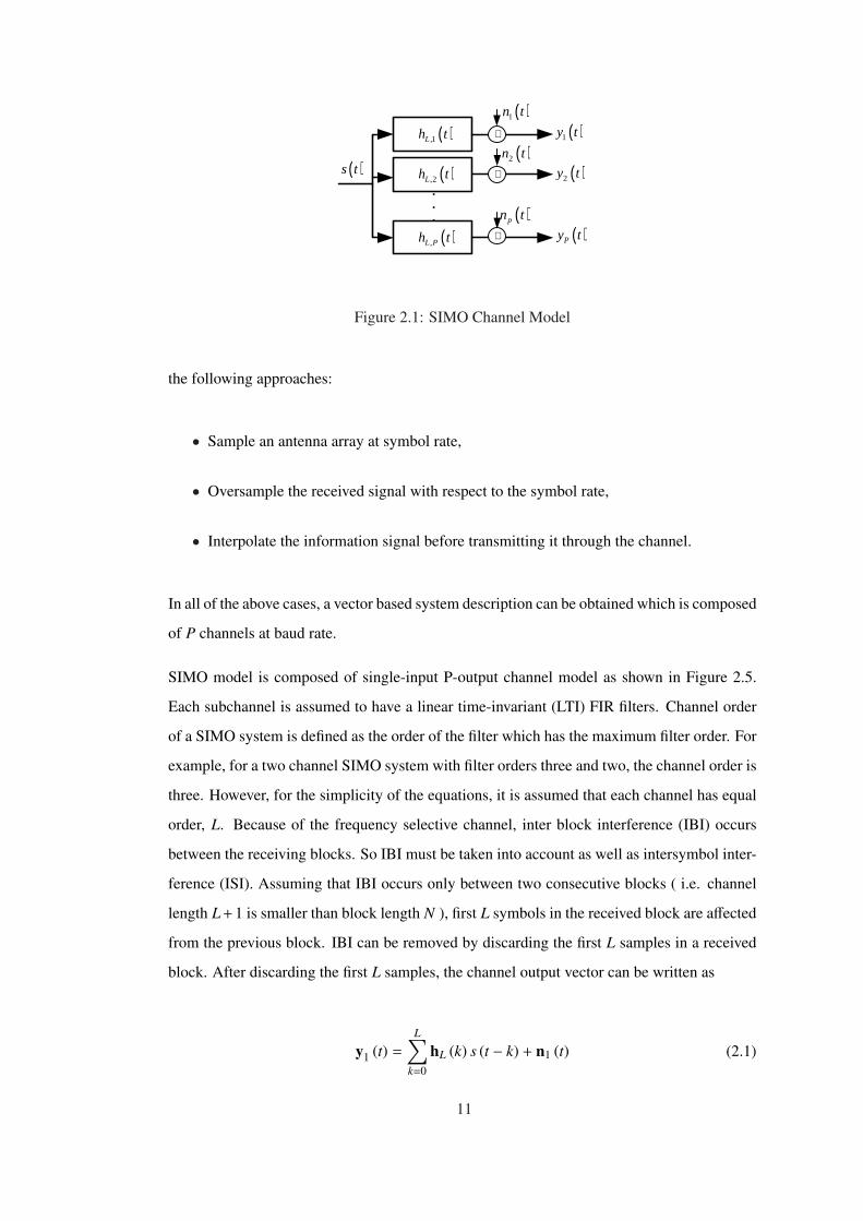
10

.

.

.

( )1y t

( )2y t

( )Py t

( )s t

( ),1Lh t

( ),2Lh t

( ),L Ph t

+

+

+

( )1n t

( )2n t

( )pn t

Figure 2.1: SIMO Channel Model

the following approaches:

• Sample an antenna array at symbol rate,

• Oversample the received signal with respect to the symbol rate,

• Interpolate the information signal before transmitting it through the channel.

In all of the above cases, a vector based system description can be obtained which is composed

of P channels at baud rate.

SIMO model is composed of single-input P-output channel model as shown in Figure 2.5.

Each subchannel is assumed to have a linear time-invariant (LTI) FIR filters. Channel order

of a SIMO system is defined as the order of the filter which has the maximum filter order. For

example, for a two channel SIMO system with filter orders three and two, the channel order is

three. However, for the simplicity of the equations, it is assumed that each channel has equal

order, L. Because of the frequency selective channel, inter block interference (IBI) occurs

between the receiving blocks. So IBI must be taken into account as well as intersymbol inter-

ference (ISI). Assuming that IBI occurs only between two consecutive blocks ( i.e. channel

length L + 1 is smaller than block length N ), first L symbols in the received block are affected

from the previous block. IBI can be removed by discarding the first L samples in a received

block. After discarding the first L samples, the channel output vector can be written as

y1 (t) =

L∑

k=0

hL (k) s (t − k) + n1 (t) (2.1)

11

where

y1 (t) =

[y1 (t) y2 (t) · · · yP (t)

]T(2.2)

hL (k) =

[hL,1 (k) hL,2 (k) · · · hL,P (k)

]T(2.3)

n1 (t) =

[n1 (t) n2 (t) · · · nP (t)

]T(2.4)

The P× 1 vectors, y1 (t), hL (k) , and n1 (t) are the received signals, channel impulse response

and additive noise respectively. yi (t), hi (k), and ni (t) are the scalar values of the output

signal, channel impulse response and additive noise for the ith channel respectively. The

matrix formulation for the same model can be given as,

y1 (t) = H1sL+1 (t) + n1 (t) (2.5)

where,

H1 =

[hL (0) hL (1) · · · hL (L)

](2.6)

sL+1 =

[s (t) · · · s (t − L)

]T(2.7)

System output can be modified to include M samples for each channel and the following

equation can be written,

yM (t) = HMsM+L (t) + nM (t) (2.8)

where

yM (t) =

[yT

1 (t) · · · yT1 (t − M + 1)

]T(2.9)

nM (t) =

[nT

1 (t) · · · nT1 (t − M + 1)

]T(2.10)

sM+L (t) =

[s (t) · · · s (t − L − M + 1)

]T(2.11)

HM =

hL (0) · · · hL (L). . . · · · . . .

hL (0) · · · hL (L)

(2.12)

The MP× (M + L) dimensional block Toeplitz matrix, HM, is channel matrix. Equation (3.8)

can be written compactly as,

Y = HMS + N (2.13)

12

where,

Y =

[yM(t) yM(t + 1) · · · yM(t + N − 1)

](2.14)

S =

[sM+L(t) sM+L(t + 1) · · · sM+L(t + N − 1)

](2.15)

N =

[nM(t) nM(t + 1) · · · nM(t + N − 1)

](2.16)

The goal is to estimate the unknown channel parameters from the observation data.

2.3 Channel Identifiability

The techniques used for the estimation of SIMO channel coefficients in a blind manner can at

best identify the channel up to a complex scale factor. To ensure the channel identification in

SIMO channels, channel diversity must be satisfied. When the channels are modeled as FIR

filters, then channel diversity means that no common zeros exist, or in other words, they are

coprime. If the channels are not coprime, there exists a common zero and that zero can not

be distinguished from the zeros of the input. Hence, we can not identify the channel without

knowing the input. The identifiability of the channel can also be defined through the channel

matrix, HM. If the channel matrix is full column rank then the channel is said to be identifiable

[2]. The channel matrix is full column rank if,

• The subchannels have no common zero.

• M is greater than (M + L)/P, so that the channel matrix is a tall matrix.

• At least one channel has an order of L and hL,k , 0 ∀k.

The channel identifiability condition determines whether the channel can be obtained in a

blind manner. There are also certain conditions that should be satisfied for the use of the

blind channel identification algorithms. The key condition that is applicable to most of the

algorithms is about the complexity of the input signal. If the outputs of the subchannels do

not carry enough information , the channel filters can not be obtained. Such a case arises

when a constant or a periodic signal is sent. Linear complexity [29] is one of the criteria in

order to decide whether the signal carry enough information. Linear complexity measures the

predictability of a finite-length deterministic sequence.

13

Definition:[7] The linear complexity of a sequence {s(t)}nt=0 is defined as the smallest value

of c for which there exists {λ j} such that

s(t) = −c∑

j=1

λ js(t − j) t = s, ..., n (2.17)

Let us consider a Toeplitz matrix, Sc, given by

Sc =

s(c) s(c − 1) · · · s(0)

s(c + 1) s(c) · · · s(1)...

... · · · ...

s(n) s(n − 1) · · · s(n − c)

(2.18)

If s(t) has linear complexity c or greater, then Sc has full column rank. Hence the sample

covariance of the vector s(t) =

[s(t) s(t − 1) · · · s(t − c)

]has full rank. On the other

hand, if s(t) has linear complexity less than c, Sc is rank deficient.

2.4 Subspace Method

The subspace method [6] exploits the low rank data model with the assumptions on noise

and source signal characteristics to identify the unknown parameters. In a low rank data

model, observation vectors belong to a certain subspace of the complex measurement space.

Generated SIMO channel model has low rank structure when the channel matrix HM has full

column rank.

yM(t) = HMsM+L(t) + nM(t) (2.19)

If the length of the temporal window, M, is chosen greater than (L + 1 − P)/(P − 1), then

channel matrix, HM , will have more rows than columns. And the columns of HM are linearly

independent if and only if the channels are coprime, in other words they do not have common

zeros.

In the case of noiseless observations, the observation vectors, yM(t), are exact linear combi-

nation of the columns of HM. Therefore the noiseless observation vectors are the elements

of the vector space which is spanned by the columns of HM . Since HM is a tall matrix, its

columns do not span the overall measurement space. The vector space, which is spanned by

14

the columns of channel matrix (i.e. range space of HM ), is a subspace of complex measure-

ment space and it is called as the signal subspace. The orthogonal complement of the signal

subspace, which is the left null space of HM , is called noise subspace. So the measurement

space is composed of these two orthogonal subspaces.

Measurement space = Noise subspace⊥⊕ S ignal subspace (2.20)

The dimension of the signal subspace is equal to the number of linearly independent columns

of HM. Since HM has full column rank, it is equal to the number of columns which is M + L.

It is possible to determine the signal and noise subspaces by collecting a number of observa-

tion vectors at the receiver, i.e.,

Y = HMS (2.21)

If the input data matrix, S (whose size is given as (M +L)×N ), is wide and full row rank, then

Y = HMS is a low rank factorization. This condition is provided by the assumption on the

linear complexity of the input signal, which should be greater than M + L. The columns of Y

are spanned by the columns of the channel matrix and it has nonempty nullspace with dimen-

sion of MP− (M + L) as a result of low rank factorization. Denoting the MP× (MP − M − L)

matrix Un as the left singular vectors of Y, which corresponds to the noise subspace,then

UHn HM = 0 (2.22)

Where subindex n used in Un is used to clarify that the matrix belongs to the noise subspace.

For the signal subspace Us is used. The channel matrix is identifiable up to a scalar complex

factor from the above equation. Since the channel matrix is identifiable up to a complex factor,

one parameter of h is fixed (i.e. say c). Under this consideration, vectorized channel matrix

can be written as,

vec(HM) = Φhhc + ah (2.23)

where Φh is a selection matrix containing only zeros and ones, hc is the parameter vector

containing the channel parameters except the fixed parameter. ah comes from the fixed pa-

rameter and it contains the fixed complex parameter and zeros. Applying (2.23) into (2.22) it

is obtained that,

vec[UH

n HM]

= Ψchc + bh (2.24)

15

where

Ψc = (I ⊗ UHn )Φh, bh = (I ⊗ UH

n )ah (2.25)

and ⊗ indicates the Kronecker product. An estimate of hc in least square sense can be found

by the following minimization,

hc = arg minhc

(Ψchc + bh)T (Ψchc + bh) (2.26)

Minimizing the cost function in (2.26) with respect to hc results in the estimated channel

coefficients.

hc = − (Ψc)† bh (2.27)

When there is no noise, subspace method produces the exact channel using the finite number

of samples. Therefore the subspace method has finite sample convergence property. It is an

important property for blind channel identification methods in the sense of the speed of the

convergence, especially in packet transmission systems where only a small number of samples

is available for processing.

Subspace method is not robust against the modeling errors, especially when the channel ma-

trix is approximately singular (i.e. Channel zeros are close to each other). Furthermore sub-

space method requires exact channel order. It is performance is not acceptable for under-

overestimated channel orders. Therefore channel order must be estimated using one of the

techniques in the literature.

2.5 Least Squares Smoothing Method

LSS method [7, 3] is based on the isomorphic relation between the input and output subspace.

It is shown that the channel order and channel impulse response are uniquely determined

by the least squares smoothing error when the isomorphism between the input and output

subspaces is considered.

Since no assumption is made about the statistics of the input signal, LSS method is considered

as a deterministic method. It has finite convergence property which is an important property

especially for packet transmission system where the channel must be estimated in a limited

time interval. The most striking property of the LSS over the other deterministic blind channel

identification methods may be the estimation of the channel order jointly with the channel

16

impulse response. Furthermore LSS method is more robust to modeling errors, i.e., when the

channel matrix is approximately singular.

Considering the isomorphic relation between the input and output subspaces, we first consider

the estimation of the channel from the input subspaces. By projecting the output data into the

punctured input subspace Z, the channel is obtained from the least squares projection error.

Since the input subspace is not directly available , the punctured input subspace Z is obtained

from the output subspaces by exploiting the isomorphic relation between the input and output

subspaces. When Z is constructed from the channel output by using the isomorphism between

the input and output subspaces, this projection is called smoothing. In joint order detection

and channel estimation, the smoothing error is minimized by jointly choosing the channel

order and channel parameters.

2.5.1 Assumptions and Properties

There are two basic assumptions for the LSS [7, 3]. One is about the system, the other one is

about the input signal. These are given below.

A1: Channel disparity condition: The subchannel transfer functions do not share common

zeros, and there exists M > W0 such that HM has full column rank. W0 is the smallest value

of M which makes the channel matrix a tall matrix.

The following property reveals the equivalence of the input and output subspaces and it plays

a critical role in smoothing approach for the channel estimation. Before that, let us define

input and output subspaces spanned by p consecutive row (block row) vectors as

S t,p = sp{

st · · · st−p+1

}= R

st st+1 · · ·...

......

st−p+1 st−p+2 · · ·

)

(2.28)

Xt,p = sp{

xt · · · xt−p+1

}= R

xt xt+1 · · ·...

......

xt−p+1 xt−p+2 · · ·

(2.29)

Where the row vector st is given as, st =

[s(t) s(t + 1) · · ·

], and noiseless observation

17

matrix is given as xt =

[x1(t) x1(t + 1) · · ·

]. R {A} indicates the space spanned by the

rows of a matrix A. The above equations can also be written for spanning |p| future data

vectors in case of p < 0 such as,

St+p,p = St,−p (2.30)

Property 1: Under disparity condition, there is an isomorphic relation between input and

output (noiseless) subspaces

Xt,M = St,M+L (2.31)

In other words, Xt,M is isomorphic to St,M+L with isomorphism HM .

In a linear system, input space may not be seen from the output space, that is some information

may be lost. Therefore, in general Xt,M ⊆ S t,M+L for a fixed M. On the other hand, with A1, all

the information of the input space is contained in the output space. Such a relation between

the input and output subspaces enables us to use the output subspace instead of direct use

of the input subspace to estimate the channel. An interesting point is that, even in case of

common zeros Xt,M may still be a good approximation of St,M. Therefore, it is more robust

against common zeros compared to Subspace method [3].

Another important assumption is about the input signal. To ensure the channel identifiability,

input signal must carry enough information. In other words, it must be sufficiently complex

to identify the channel from the observation data. This requirement is imposed by the linear

complexity of the signal.

A2: Linear Complexity: [3] The input sequence s(t) has linear complexity greater than

2Wo + 2L.

The reason of the assumption A2 will be clearer in the following section when the necessary

number of input symbols to identify the channel is discussed.

2.5.2 Least Squares Smoothing Algorithm

In this section, we introduce the linear least squares smoothing channel estimation by exploit-

ing the isomorphic relation between input and output (noiseless) spaces. First, the estimation

of channel from the input subspace is considered.

18

By projecting the output data into the input subspace, the channel is obtained from the least

squares projection error. But normally input subspace is not directly available from observa-

tion. Therefore, instead of using input subspace, output subspace can be used by exploiting

the isomorphic relation between the input and output subspace. So, the second step will be to

identify the channel from the output subspace.

2.5.2.1 Channel Identification from Input Subspace

Consider L+1 consecutive output block row vectors xt+L, ..., xt . From (A.1) we have,

xt+L = h(0)st+L + h(1)st+L−1 + · · · + h(L)st (2.32)

xt+L−1 = h(0)st+L−1 + · · · + h(L − 1)st + h(L)st (2.33)...

. . . (2.34)

xt = h(0)st + · · · + h(L)st (2.35)

The aim is to identify h(0), ...,h(L) up to a scaling factor from xt+L,..., xt . One way is to

Zti |~sh

tish

Zit |ˆ +x

Zit |~

+x ∑ ≠= −+L

ikk kitk,0

)( sh Z

∑ = −++ = L

k kitit k0

)( shx

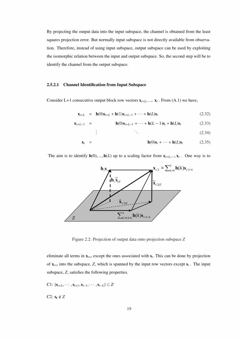
Figure 2.2: Projection of output data onto projection subspace Z

eliminate all terms in xt+i except the ones associated with st. This can be done by projection

of xt+i into the subspace, Z, which is spanned by the input row vectors except st . The input

subspace, Z, satisfies the following properties.

C1: {st+L, · · · , st+1, st−1, · · · , st−L} ⊂ Z

C2: st < Z

19

As illustrated in figure 2.2, xt+i is composed of two components: one is inside the punctured

subspace Z, which equals toL∑

k=0,k,ih(k)st+i−k, the other one is outside the Z space which equals

to hist. The projection error of xt+i into Z space denoted by xt+i|Z is

xt+i|Z = hist|z (2.36)

Consequently, we have

E =

xt+L|Z...

xt|Z

= hst|z (2.37)

Note that E is a rank one matrix whose columns and rows are spanned by h and st|Z respec-

tively. The channel can be identified from the projection error matrix E by several ways. One

way is to obtain the singular value decomposition (SVD) of E or the sample covariance of E.

The eigenvector corresponding to the maximum eigenvalue spans the column space of E and

so h. Therefore, this eigenvector can be taken as an estimate of h.

2.5.2.2 Channel Identification from Output Subspace

In the previous section, it is shown that channel can be identified from the projection errors

of xt+L, ..., xt into the projection subspace Z satisfying the properties C1 and C2. Using the

isomorphic relation between the input and output subspaces, the input subspace, Z, can be

constructed from the output subspace, so that direct use of the input sequence is avoided.

Under C1 and C2, the projection subspace is defined as,

Z = St−1,p ∪ St+1,−p

for any p ≥ L.With the isomorphic relation between the input and output subspaces described

in property 1, we have

Z = St−1,M+L ∪ St+1,−(M+L) = Xt (2.38)

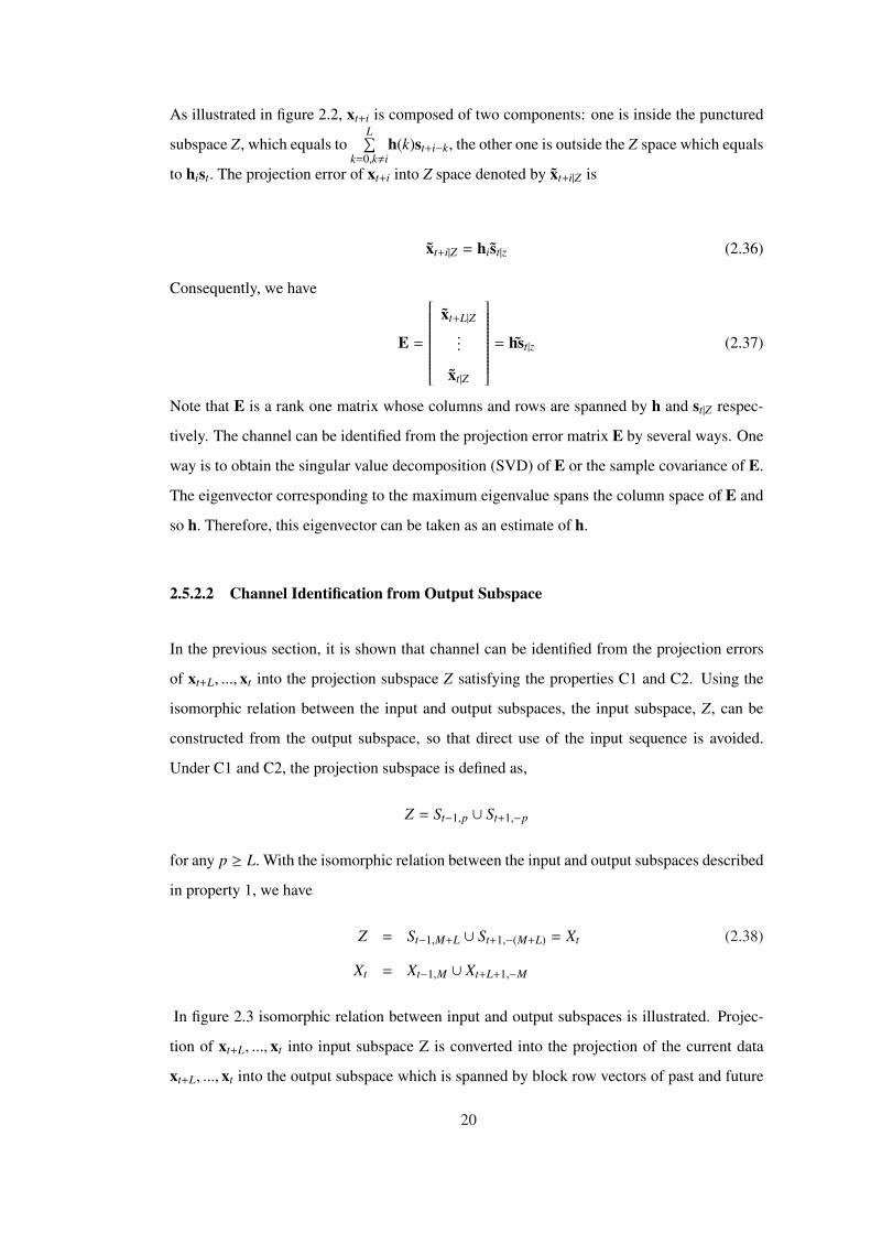
Xt = Xt−1,M ∪ Xt+L+1,−M

In figure 2.3 isomorphic relation between input and output subspaces is illustrated. Projec-

tion of xt+L, ..., xt into input subspace Z is converted into the projection of the current data

xt+L, ..., xt into the output subspace which is spanned by block row vectors of past and future

20

LWtS +− ,1

WtX ,1−

)(,1 LWtS +−+

WLtX −++ ,1

Wt−x 1−tx

tx Lt+x 1++Ltx WLt ++x

LWt −−s 1−ts 1+ts LWt ++s ts

PAST DATA

PAST DATA

FUTURE DATA

FUTURE DATA

CURRENT DATA

INPUT SUBSPACE

OUTPUT SUBSPACE

)0(h )(Lh

Z

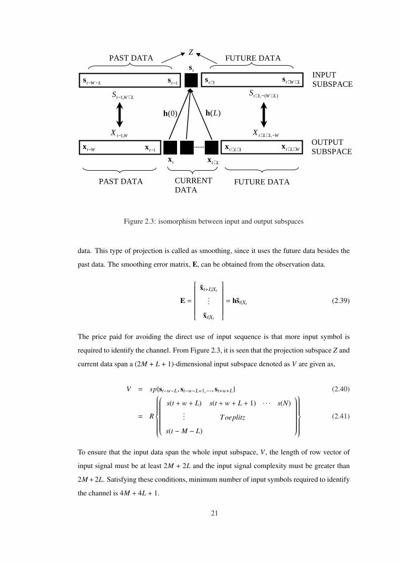
Figure 2.3: isomorphism between input and output subspaces

data. This type of projection is called as smoothing, since it uses the future data besides the

past data. The smoothing error matrix, E, can be obtained from the observation data.

E =

xt+L|Xt

...

xt|Xt

= hst|Xt (2.39)

The price paid for avoiding the direct use of input sequence is that more input symbol is

required to identify the channel. From Figure 2.3, it is seen that the projection subspace Z and

current data span a (2M + L + 1)-dimensional input subspace denoted as V are given as,

V = sp{st−w−L, st−w−L+1,..., st+w+L} (2.40)

= R

s(t + w + L) s(t + w + L + 1) · · · s(N)... Toeplitz

s(t − M − L)

(2.41)

To ensure that the input data span the whole input subspace, V , the length of row vector of

input signal must be at least 2M + 2L and the input signal complexity must be greater than

2M + 2L. Satisfying these conditions, minimum number of input symbols required to identify

the channel is 4M + 4L + 1.

21

2.5.3 General Formulation of LSS

Up to now, channel order is assumed to be known. In this section a general formulation is

given when the channel order is not known. For this purpose, projection space, Z, is redefined

according to an arbitrary channel order l as follows.

Zl = Xt−1,M ∪ Xt+l+1,−M (2.42)

= Xt−1,M ∪ Xt+l+M,M

Because of the isomorphic relation between the output and input subspaces,

Zl = S t−1,L+M ∪ S t+l+M,L+M (2.43)

Therefore,

Zl =

sp {st−L−M , ..., st, ..., st+l+M} , l < L

sp{st−L−w, ..., st−1} ∪ sp{st+l−L+1, ..., st+l+M} , L ≤ l

Projecting xt+i, i = 0, ..., l, into Zl, following results are obtained through Theorem-1 in [3].

Let El be least squares smoothing error matrix defined by

El =

xt+l|Zl

...

xt|Zl

(2.44)

then,

El =

0 , l < L

Hl(h)

st+l−L|Zl

st|Zl

, L ≤ l

(2.45)

where

Hl(h) =

h(L)...

. . .

h(0). . . h(L). . .

...

h(0)

(2.46)

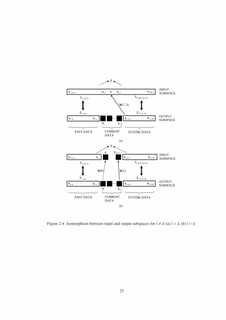
The above result is the center of the approach especially when the channel order is unknown.

In the case of l < L (Figure 2.4.a), the projection space Zl includes st . Since xt, ..., xt+l all

22

LWtS +− ,1

WtX ,1−

)(,1 LWWtS +++

WltX −++ ,1

Wt−x 1−tx

tx lt+x 1++ltx Wlt ++x

LWt −−s 1−ts 1+ts lWt ++s ts

PAST DATA FUTURE DATA CURRENT DATA

INPUT SUBSPACE

OUTPUT SUBSPACE

)1( +lh

Z

(a)

LWtS +− ,1

WtX ,1−

)(,1 LWWtS +++

WltX −++ ,1

Wt−x 1−tx

tx lt+x 1++ltx Wlt ++x

LWt −−s 1−ts lWt ++s ts

PAST DATA FUTURE DATA CURRENT DATA

INPUT SUBSPACE

OUTPUT SUBSPACE

)(Lh )0(h

1−−+ Llts

Llt −+s Wlt ++s

Z

(b)

Figure 2.4: Isomorphism between input and output subspaces for l , L (a) l < L (b) l > L

23

includes st, they also lie in the projection space. As a result, when xt, ..., xt+l are projected onto

Zl, no projection error exists, i.e., El = 0. When l = L, we have the case described in previous

section, where the channel vector spans the column space of El. When we choose the channel

order greater than L (Figure 2.4.b), sM+1, .., sM+l−L are not in Zl. Since each of xt, ..., xt+l does

not lie in Zl, they contribute the least squares smoothing error which is formulated in (2.45).

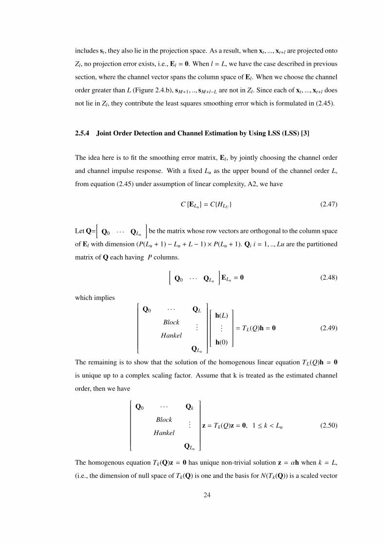
2.5.4 Joint Order Detection and Channel Estimation by Using LSS (LSS) [3]

The idea here is to fit the smoothing error matrix, El, by jointly choosing the channel order

and channel impulse response. With a fixed Lu as the upper bound of the channel order L,

from equation (2.45) under assumption of linear complexity, A2, we have

C{ELu

}= C{HLU } (2.47)

Let Q=

[Q0 · · · QLu

]be the matrix whose row vectors are orthogonal to the column space

of El with dimension (P(Lu + 1) − Lu + L − 1) × P(Lu + 1). Qi i = 1, .., Lu are the partitioned

matrix of Q each having P columns.

[Q0 · · · QLu

]ELu = 0 (2.48)

which implies

Q0 · · · QL

Block

Hankel

...

QLu

h(L)...

h(0)

= TL(Q)h = 0 (2.49)

The remaining is to show that the solution of the homogenous linear equation TL(Q)h = 0

is unique up to a complex scaling factor. Assume that k is treated as the estimated channel

order, then we have

Q0 · · · Qk

Block

Hankel

...

QLu

z = Tk(Q)z = 0, 1 ≤ k < Lu (2.50)

The homogenous equation Tk(Q)z = 0 has unique non-trivial solution z = αh when k = L,

(i.e., the dimension of null space of Tk(Q) is one and the basis for N(Tk(Q)) is a scaled vector

24

of h ). Otherwise there is only trivial solutions ( i.e., since Tk(Q) is full column rank, only

element in null space of Tk(Q) is null vector and as a result there is only one solution z = 0),

[3]. Under this statement the criteria is,

{L, h} = arg mink,‖h‖=1

‖Tk(Q)h‖ (2.51)

The above equation has a closed form solution involving the left singular vector of Tk(Q)

corresponding to the smallest singular value.

2.5.5 Algorithm:

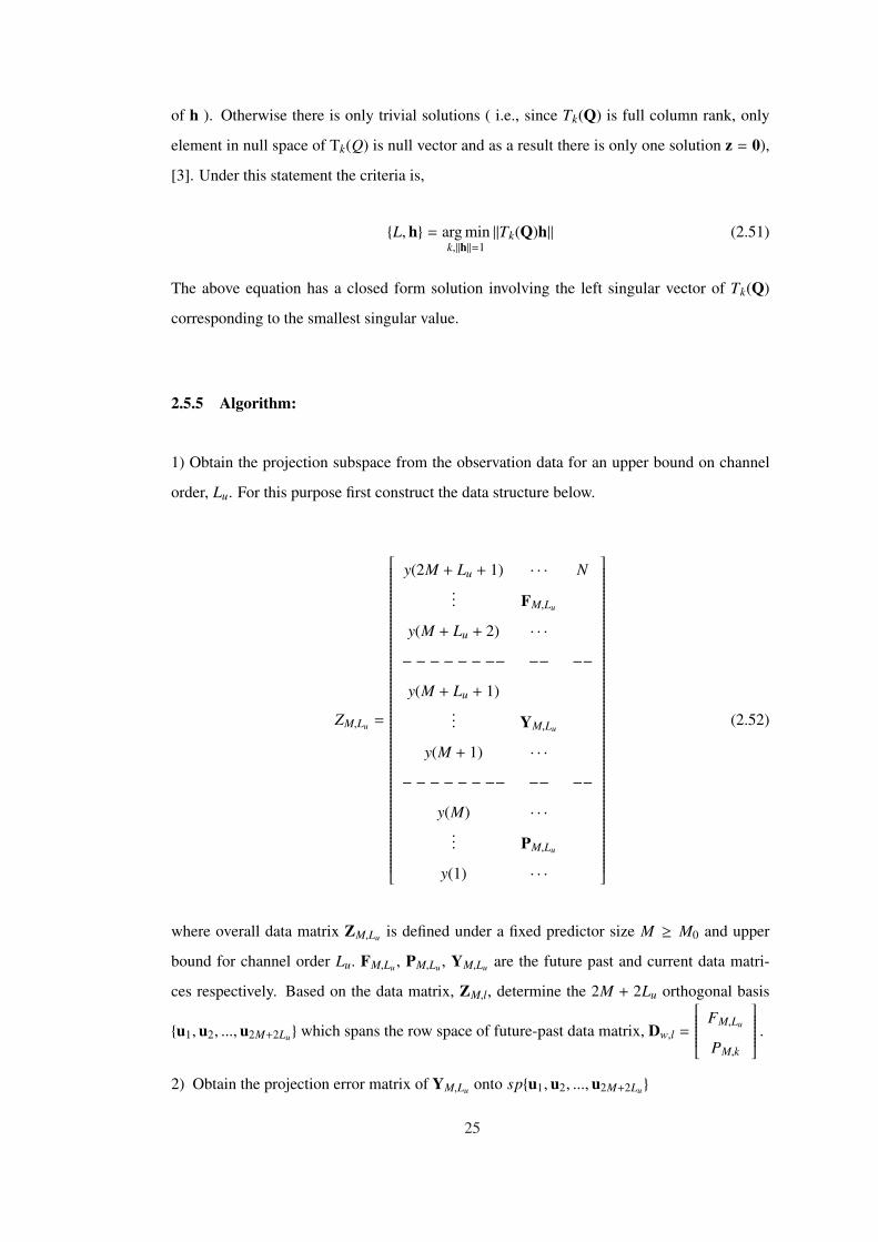
1) Obtain the projection subspace from the observation data for an upper bound on channel

order, Lu. For this purpose first construct the data structure below.

ZM,Lu =

y(2M + Lu + 1) · · · N... FM,Lu

y(M + Lu + 2) · · ·− − − − − − −− −− −−y(M + Lu + 1)

... YM,Lu

y(M + 1) · · ·− − − − − − −− −− −−

y(M) · · ·... PM,Lu

y(1) · · ·

(2.52)

where overall data matrix ZM,Lu is defined under a fixed predictor size M ≥ M0 and upper

bound for channel order Lu. FM,Lu , PM,Lu , YM,Lu are the future past and current data matri-

ces respectively. Based on the data matrix, ZM,l, determine the 2M + 2Lu orthogonal basis

{u1,u2, ..., u2M+2Lu} which spans the row space of future-past data matrix, Dw,l =

FM,Lu

PM,k

.

2) Obtain the projection error matrix of YM,Lu onto sp{u1, u2, ..., u2M+2Lu}

25

ELu = YM,Lu − YM,LuUHU , U =

u1...

u2M+2Lu

(2.53)

3) For each 1≤ k ≤ Lu, treated as the estimated channel order, let Q =

[Q0 · · · Ql

]be a

matrix whose rows are the smallest P(Lu +1)−Lu +k−1 left singular vectors of ELu and form

Tk(Q) =

Q0 · · · Qk

Block

Hankel

...

QLu

4) Joint order and channel estimation:

{L, h} = arg mink,‖h‖=1

‖Tk(Q)h‖

Left singular vector of Tk(Q) corresponding to the smallest singular value can be taken as a

solution.

2.6 Linear Prediction Method

Linear prediction method is first proposed by Slock [14], it is based on the fact that moving

average (MA) SIMO channel output can also be represented as AR process, whose innovation

is the SIMO channel input. Yule-Walker (YW) equations are solved to obtain zero delay zero

forcing equalizer. Channel impulse response is derived from equalizer equations. It uses

SOS to construct the YW equations and needs pseudoinverse of the covariance matrix. LP

algorithm uses statistical characteristic of the inputs and based on the second order statistics.

It assumes that, the channel input signal is Gaussian distributed white signal. Therefore it

is not a deterministic algorithm as opposed to SS, CR and LSS algorithms. Therefore in

noise free case it does not give the exact channel coefficients from finite number of samples.

As cited in [30] the most striking property of the LP algorithm is the robustness to channel

order overestimation, since the ma order AR process can be treated as mthb order AR process

26

when ma > mb. However in [4] and [18], it is claimed that it is not the case when the

estimated SOS is used and the channel order is over estimated more then two degrees. It is

understood that this technique is sensitive to observation noise and its performance depends

on the channel statistics [16]. Therefore a new algorithm which is claimed to be robust to

channel order overestimation is proposed in [16]. It turns out that this algorithm outperforms

the LP algorithm in [14]. In [17] SNR optimum linear prediction equalizer is proposed and

it is shown that [17] and [16] have the same asymptotically behavior whereas [17] performs

better especially for short data lengths. In this section, a review of the original LP method

[15] and the modified LP method (MLP) [17] is given.

Referring to the section 2.2, the channel output vector, y1(t), which is composed of single

samples from each channel outputs, is given as follows in noise free case.

y1 (t) =

L∑

k=0

hL (k) s (t − k). (2.54)

This equation can also be written as follows.

y1(t) = H1(z)s(t) (2.55)

Where, H1(z) =L∑

k=0hL(k)z−k. Under channel identifiability condition, according to the Bezout

Identity [37], there exists inverse filter matrix G(z) such that,

G(z)H1(z) = I (2.56)

i.e.,

G(z)y1(t) = s(t) (2.57)

Where G(z) =K+1∑k=0

gkz−k and gk =

[g1(k) · · · gP(k)

]T. gi(k) is the kth coefficient of the ith

equalizer filter.

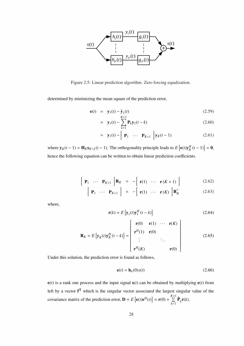
The equation (2.57) implies that y1(t) is an AR process. Therefore linear prediction filter

exits for y1(t). For the Kth order linear prediction, the estimated channel output vector y1(t) is

written as follows,

^y1(t) =

K+1∑

k=1

Pky1(t − k) (2.58)

where Pk are the prediction filter coefficient vector. The prediction filter coefficients can be

27

+

1( )g t

( )Ph t

1( )h t1( )y t

( )Py t( )Pg t

( )s t ( )s t

Figure 2.5: Linear prediction algorithm. Zero forcing equalization.

determined by minimizing the mean square of the prediction error,

e(t) = y1(t) − ^y1(t) (2.59)

= y1(t) −K+1∑

k=1

Pky1(t − k) (2.60)

= y1(t) −[

P1 · · · PK+1

]yK(t − 1) (2.61)

where yK(t − 1) = HKsK+L(t − 1). The orthogonality principle leads to E{e(t)yH

K (t − 1)}

= 0,

hence the following equation can be written to obtain linear prediction coefficients.

[P1 · · · PK+1

]RK = −

[r(1) · · · r (K + 1)

](2.62)

[P1 · · · PK+1

]= −

[r(1) · · · r (K)

]R†K (2.63)

where,

r(k) = E{y1(t)yH

1 (t − k)}

(2.64)

RK = E{yK(t)yH

K (t − k)}

=

r(0) r(1) · · · r(K)

rH(1) r(0)...

. . .

rH(K) r(0)

(2.65)

Under this solution, the prediction error is found as follows,

e(t) = hL(0)s(t) (2.66)

e(t) is a rank one process and the input signal s(t) can be obtained by multiplying e(t) from

left by a vector fT which is the singular vector associated the largest singular value of the

covariance matrix of the prediction error, D = E{e(t)eH(t)

}= r(0) +

K+1∑k=1

Pkr(k).

28

fT e(t) = s(t) (2.67)

Using the above equation, equalization filter G(z) can be obtained as follows.

fT e(t) = s(t) (2.68)

fT

y1(t) −K+1∑

k=1

Pky1(t − k)

= s(t) (2.69)

fT P(z)y1(t) = s(t) (2.70)

Hence,

G(z) = fT P(z) (2.71)

where, P(z) = I −K+1∑k=1

Pkz−k.

The channel coefficients can be obtained as a follows,

h(k) = E {y1(t)s(t − k)} = E{y1(t)G(z)y1(t − k)

}(2.72)

in matrix form,

h =

r(0) r(1) · · · r(K)

r(1) r(2) 0...

...

r(K) 0 · · · 0

GT (2.73)

The main problem of LP method is that prediction error increases when the first channel

coefficient is small. With modified LP, [17] this problem is solved in a certain extent and

SNR optimum LP solution is obtained. The main difference from LP stems from obtaining

f and the matrix P, which is the matrix form of P(z). In MLP, P matrix obtained in LP is

modified such that its columns are orthogonal. In the same manner, f is the singular vector

associated the largest singular value of PHRKP. MLP methods is more robust channel order

overestimation and has better performance when the channel has small tail coefficients.

2.7 Channel Order Estimation

Blind channel order estimation is a critical task required for blind system identification. De-

terministic channel estimation algorithms such as SS, CR, and LSS require exact channel

29

order information. There are several algorithms for the channel order estimation in the lit-

erature. Minimum Description Length (MDL) [19] and Akaike Information Criteria (AIC)

[20] algorithms are based on the information theoretic criteria. These algorithms require long

observations for accurate extraction of the statistical parameters. It is known that both of these

algorithms are very sensitive to deviation from idealized Gaussian white noise signal, number

of observations and variations in SNR [4]. Therefore they are not robust approaches and their

performances are not consistent and reliable in realistic scenarios.

In practice, channel impulse response contains long leading and trailing tails as in the case of

microwave channels. Usually the channel is modeled to contain only the significant part of the

impulse response for those cases. The order of the significant part is defined as the effective

channel order whereas the true channel order indicates the whole channel filter including the

tails. In [22], it is shown that when the channel model includes a part of the tail, the estimation

performance of the subspace and least squares algorithms decrease dramatically. In [5] a

channel order estimation algorithm is proposed for the effective channel order estimation.

This algorithm is based on numerical analysis arguments and essentially consider the gap

between the two consecutive eigenvalues of the estimated covariance matrix.

Most of the cost functions derived for channel order estimation monotonically decreases as the

channel order increases, which makes it hard to find the channel order. This problem is tried

to be overcome by using an empirically chosen penalty coefficient [23]. This penalty term

leads to over or underestimation in many of the information theoretic techniques. In [24], a

new cost function is proposed. This cost function is obtained by combining two cost functions

due to channel identification (ID) and channel equalization (EQ), and hence ID+EQ algorithm

is obtained. The main feature of this cost function is its ”concave - like” shape. Therefore

channel order estimation can be performed by finding the global minimum. ID+EQ algorithm

is a deterministic method and has finite convergence property as JLSS. It is claimed that it olso

perform well in finding the effective channel order.

In this section, channel order estimation algorithms MDL, AIC, Liavas, and ID+EQ algo-

rithms which are referenced throughout the thesis are summarized.

30

2.7.1 Akaiki Information Criteria (AIC) [20]

AIC is basically a rank determination method. It uses the covariance matrix to determine

the dimension of the signal or noise subspace to identify the channel length. It assumes that

the channel input is a Gaussian distributed white signal. Under this assumption, correlation

matrix of channel the output can be written as follows:

Ry = E{yM(t)yH

M(t)}

= σ2sHMHH

M + σ2vI (2.74)

The SVD of Ry is given as follows, (assuming that channel identifiability condition is hold),

Ry =

[Us

... Un

]

λ1 + σ2v

. . .

λM+L + σ2v

σ2v

. . .

σ2v

Us

Un

(2.75)

whereσ2s andσ2

v are the channel input signal and noise variances respectively. Us is the eigen-

vector matrix corresponding the eigenvalues λ1 + σ2v . . . λM+L + σ2

v and its columns span the

signal space. Un is the eigenvector matrix corresponding eigenvalues equal to noise variance,

σ2v and its columns span the noise space. If one can find the dimension of one of these spaces,

channel order can be found. In noise free case, the number of nonzero eigenvalues give the

dimension of the signal space, which is equal to the number of columns of the channel matrix.

Subtracting the value of M (which is a known value) from the found signal subspace dimen-

sion, the channel order is determined. However in noisy case, it is not so easy to separate

the signal and noise spaces from each other, and the true data covariance matrix is not acces-

sible in practice from finite number of samples. AIC algorithm uses statistical information

to find the dimension of signal/noise spaces or equivalently the rank of the channel output

matrix. AIC finds the channel order via maximum likelihood (ML) optimization and selects

the model that minimizes,

AIC = −2 log(

f(

yM(t) · · · yM(t + N − 1) |θ))

+ 2k (2.76)

where f(

yM(t) · · · yM(t + N − 1) |θ)

is the parameterized probability densities and θ is

the ML estimate of the parameter vector θ. Assuming that the observed vectors {yM(t + k)}Nk=1

31

are zero mean i.i.d. Gaussian random vectors (note that, this is not the case for the channel

identification problem, because the channel output samples are correlated as a consequence

of FIR channel impulse response.), AIC obtains the dimension of signal space by minimizing

the cost function given below [20], when the empirical covariance matrix Ry = 1N YMYH

M is

used.

AIC(k) = −2 log

p∏i=k+1

λ1/(MP−k)i

1MP−k

MP∑i=k+1

λi

(MP−k)N

+ 2k(2MP − k) (2.77)

where λ1 ≥ λ2 ≥ · · · ≥ λMP are the eigenvalues of covariance matrix Ry. MP is the size of

the observation vector yM(t) for P channel SIMO system. Channel order is the value of k that

minimizes the cost function AIC(k).

2.7.2 Minimum Description Length (MDL) [19]

MDL is similar to the AIC and selects the model that minimizes,

MDL = − log(

f(

yM(t) · · · yM(t + N − 1) |θ))

+12

k log N (2.78)

which results the following cost function to find the dimension of signal space.

MDL(k) = − log

p∏i=k+1

λ1/(MP−k)i

1MP−k

MP∑i=k+1

λi

(MP−k)N

+12

k(2MP − k) log N (2.79)

where λ1 ≥ λ2 ≥ · · · ≥ λMP are the eigenvalues of the empirical covariance matrix Ry.

Channel order is the value of k that minimizes the cost function MDL(k).

MDL is an asymptotically consistent algorithm in contrast to the AIC. When the number of

snapshots is increased, probability of wrong detection of the channel order goes to zero [23].

It is more robust to deviation from the Gaussian assumption on the observation vectors.

2.7.3 Liavas Algorithm [4]

Liavas algorithm is proposed for the estimation of effective channel order from channel out-

puts when the channel impulse is long and includes small long channel tails. In that case, true

channel and effective channel order are different and using effective channel order to model

32

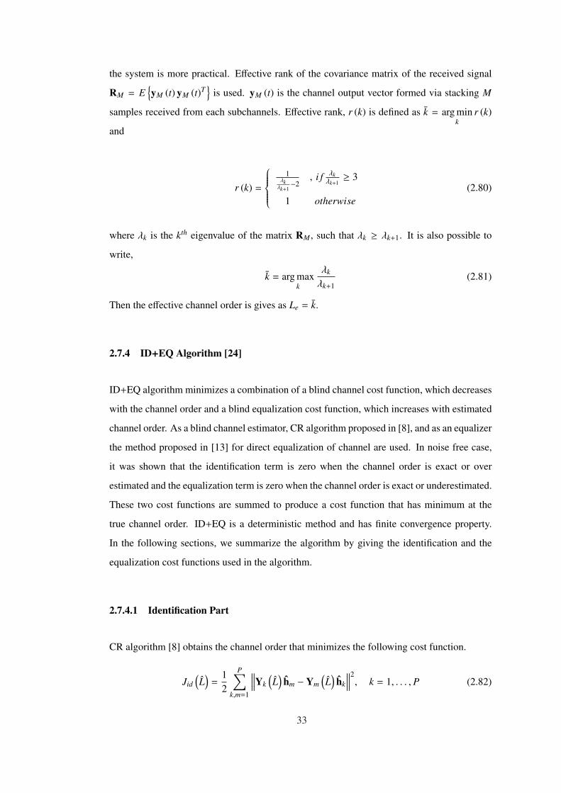
the system is more practical. Effective rank of the covariance matrix of the received signal

RM = E{yM (t) yM (t)T

}is used. yM (t) is the channel output vector formed via stacking M

samples received from each subchannels. Effective rank, r (k) is defined as k = arg mink

r (k)

and

r (k) =

1λkλk+1−2

, i f λkλk+1≥ 3

1 otherwise(2.80)

where λk is the kth eigenvalue of the matrix RM , such that λk ≥ λk+1. It is also possible to

write,

k = arg maxk

λk

λk+1(2.81)

Then the effective channel order is gives as Le = k.

2.7.4 ID+EQ Algorithm [24]

ID+EQ algorithm minimizes a combination of a blind channel cost function, which decreases

with the channel order and a blind equalization cost function, which increases with estimated

channel order. As a blind channel estimator, CR algorithm proposed in [8], and as an equalizer

the method proposed in [13] for direct equalization of channel are used. In noise free case,

it was shown that the identification term is zero when the channel order is exact or over

estimated and the equalization term is zero when the channel order is exact or underestimated.

These two cost functions are summed to produce a cost function that has minimum at the

true channel order. ID+EQ is a deterministic method and has finite convergence property.

In the following sections, we summarize the algorithm by giving the identification and the

equalization cost functions used in the algorithm.

2.7.4.1 Identification Part

CR algorithm [8] obtains the channel order that minimizes the following cost function.

Jid(L)

=12

P∑

k,m=1

∥∥∥∥Yk(L)

hm − Ym(L)

hk

∥∥∥∥2, k = 1, . . . , P (2.82)

33

where

hm =

[hL,m

(L), · · · hL,m (0)

]T(2.83)

Ym (L) =

ym (t) ym (t + 1) · · · ym(t + L

)

ym (t + 1) ym (t + 2) · · · ym(t + L + 1

)

......

. . ....

ym(t + N − L − 1

)ym

(t + N − L

)· · · ym (t + N − 1)

(2.84)

The cost function can also be written as follows,

Jid(L)

= 1 −P∑

k,m=1k,m

hHmRkmhk (2.85)

where Rkm(L)

= YHk

(L)

Ym

(L). The key point is that, when the channel order is overesti-

mated, the channel transfer functions obtained via CR algorithm are in the following form,

hk,L(t) = hk,L(t) ∗ cL−L

(t) (2.86)

That is the overestimated channel order generates common zeros besides the true channel

response hk,L(t).

-

, ( )i Lh t

0( )s t

( )iy t

( )jy t, ( )j Lh t

, ( )j Lh t

, ( )i Lh t

ˆ ( )−L Lc t

ˆ ( )−L Lc t

Figure 2.6: CR blind channel identification for SIMO channel.

In figure 2.6 this situation can be seen for two channel case. Since the extra zeros are common,

two branches of the channels are equal as in the case of exact channel order. Therefore the

cost function will be zero for the overestimated channel orders.

The channel vector, h =

[hT

1 · · · hTP

]T, that minimizes the cost function under the con-

straintP∑

k,m=1k,m

∥∥∥Ykhm∥∥∥2

= 1 (which is used to avoid nontrivial solutions) is given as the eigenvec-

tor associated the largest eigenvalue of the following generalized eigenvalue (GEV) problem:

R(L)

h =(1 − Jid

(L))

D(L)

h (2.87)

34

where

R(L)

=

0 R21(L)

· · · RP1(L)

R12(L)

0 . . ....

.... . .

. . . RP(P−1)(L)

R1P(L)

· · · R(P−1)P(L)

0

(2.88)

D(L)

=

∑Pk=2 Rkk

(L)· · · 0

.... . .

...

0 · · · ∑P−1k=2 Rkk

(L)

(2.89)

When the channel order is underestimated channel identification is not possible and Jid(L)>

0. When the channel order is overestimated, the cost function is equal to zero. When the

correct channel order is known, channel is identified up to a complex scalar and the cost

function is equal to zero.

2.7.4.2 Equalization Part

Direct equalization method proposed in [13] is used. In that method, equalization is realized

without the estimated channel coefficients. We will review the direct equalization algorithm

and give equalization cost function in this section. For this purpose, let us start with the

definition of row vectors h (n) =

[hL,1 (n) · · · hL,P (n)

], y (n) =

[y1 (n) · · · yP (n)

]

35

and matrices shown below.

Yk(L)

=

y (K + k) · · · y (k)

y (K + k + 1) · · · y (k + 1)...

. . ....

y(N − L − K + k − 1

)· · · y

(N − L − 2K + k − 1

)

(2.90)

Sk(L)

=

s (K + k) · · · s (k − L)

s (K + k + 1) · · · s (k − L + 1)...

. . ....

s(N − L − K + k − 1

)· · · s

(N − L − 2K + k − L − 1

)

(2.91)

Th =

h (0) 0 · · · 0... h (0)

. . ....

h (L)...

. . . 0

0 h (L) h (0)...

. . .. . .

...

0 · · · 0 h (L)

(2.92)

In noiseless case, SIMO system outputs can be written as follows,

Yk(L)

= Sk(L)

Th (2.93)

If Th is full row rank, there exists a matrix,W (L) =

[w0 (L) · · · wK+L (L)

]such that,

Yk(L)

W (L) = Sk (2.94)

and for k,m = 0, . . . ,K + L, this matrix will satisfy

Yk(L)

wk (L) = Ym(L)

wm (L) (2.95)

This equation is used to drive the equalization cost function which is given as,

Jeq(L)

=1

2 (K + L)

K+L∑

k,m=0

∥∥∥∥Yk(L)

wk (L) − Ym(L)

wm (L)∥∥∥∥

2(2.96)

= 1 −K+L∑

k,m=0k,m

wHk

(L)

Rkmwm

(L)

(2.97)

and with a constraintK+L∑k=0

∥∥∥∥Yk(L)

wk(L)∥∥∥∥

2= 1, and Rkm

(L)

= YHk

(L)

Ym

(L). The solution

that minimizes the cost function is given by the eigenvector associated largest eigenvalue

36

value of GEV:1

K + LR

(L)

w(L)

=(1 − Jeq

(L))

D(L)

w(L)

(2.98)

where w(L)

=

[wT

0

(L)· · · wT

K+L

(L) ]

and,

R(L)

=

0 R01(L)

· · · R0(K+L)(L)

R10(L)

0 . . ....

.... . .

. . . R(K+L−1)(K+L)(L)

R(K+L)0

(L)

· · · R(K+L)(K+L−1)(L)

0

(2.99)

D(L)

=

R00 · · · 0...

. . ....

0 · · · R(K+L)(K+L)

(2.100)

In [24] It is shown that, when the channel order is overestimated equalization is not possible

and Jeq(L)> 0. When the channel is underestimated, there are infinite number of solutions

and the input signal is obtained as s(n) =

[a0 · · · aL−L

]∗ s(n) in noise free case ( ∗

indicates the convolution operation). Therefore, the equalization cost function is equal to zero

for underestimated channel orders. When the channel order is known, channel is equalized

perfectly and equalization cost function is equal to zero in noise free case.

2.7.4.3 Combined Cost Function

The determined channel order, equalization and identification cost function are summed to

obtain a single cost function. Since both of the cost functions for the equalization and identi-

fication are limited between 0 and 1 as a result of the constraints defined on them, summation

with equal weighting is enough to construct the combined cost function for the channel order

estimation. Therefore overall cost function is,

J(L) = Jeq(L)

+ Jid(L)

(2.101)

To find the channel order, the cost function defined in (2.101) is determined for the channel

orders in the search set. The channel order that produces the minimum cost is taken as the

true channel order.

37

CHAPTER 3

BLIND CHANNEL ORDER ESTIMATION

3.1 Introduction

Channel order estimation is an important problem in many signal processing applications. In

this thesis, this problem is considered for finite impulse response (FIR) SIMO systems. In

blind estimation for SIMO systems, the main problem is to obtain the channel coefficients or

the input signal given the SIMO system outputs. The input and channel coefficients can be

estimated accurately when the channel order is known.

Incorrect channel order estimation results performance loss especially for the channel estima-

tion algorithms with finite convergence property such as SS [6], LSS [7] and cross relation

(CR) [8]. On the other hand, there are methods that work in a robust manner in case of overes-

timated channel order [32, 14, 15, 33]. The main disadvantage of such techniques is that their

performance is not as good as the SS or LSS algorithm when the true channel order is supplied

to those algorithms [15]. Therefore channel order estimation is an important problem and it

determines the performance of the channel estimation algorithms.

There are different algorithms for the channel order estimation in the literature. Minimum

Description Length (MDL) [19] and Akaike Information Criteria (AIC) [20] algorithms are

based on the information theoretic criteria. These algorithms require long observations for

accurate extraction of the statistical parameters. It is known that MDL usually performs better

than the AIC and AIC has a tendency for overestimation [4, 21]. Both of these algorithms are

sensitive to colored noise [21].

Joint channel order and channel estimation with LSS method (JLSS) is presented in [3]. It

38

is shown that JLSS can find the true channel order from finite number of samples in case of

noise free observations. Joint least squares smoothing (JLSS) [3] and ID+EQ [24] are the two

algorithms that can find the true channel order from finite number of samples in noise free

case. Until now, JLSS and ID+EQ were the only algorithm known to have finite convergence

property for the channel order estimation.

In this work, two new channel order estimation algorithms are proposed, namely the channel

output error (COE) and channel matrix recursion (CMR) algorithms. Both of these algorithms

have the finite convergence property. In other words, they find the true channel order by using

finite number of samples for noise free case. In addition, they have several distinct features

which make them practically the most effective algorithms known in the literature. Their

performances are significantly better than the alternatives for noisy observations. They are

robust to different parameters such as the number of channels, channel order and the number

of input samples. COE algorithm is computationally demanding. In return, its performance

gets better than CMR with the increase in the number of channels and the channel order. On

the other hand, CMR performs better when the number of channels and the channel order

is small. CMR has better computational efficiency than the COE algorithm. In this respect,

COE and CMR complement each other nicely.

Most of the cost functions monotonically decrease as the channel order increases, which

makes it hard to find the true channel order. This problem is tried to be overcome by us-

ing an empirically chosen penalty coefficient [23]. This penalty term leads to over or un-

derestimation in many of the information theoretic techniques. In [24], a new cost function

is proposed. This cost function is obtained by combining two cost functions due to channel

identification (ID) and channel equalization (EQ), and hence ID+EQ algorithm is obtained.

The main feature of this cost function is its ”convex - like” shape. Therefore channel order

estimation can be performed by finding the global minimum. The motivation in this thesis

is to construct a similar cost function, which allows us to obtain the channel order from the

global minimum. In this respect, channel output error is chosen as one of the cost functions.

In order to compute the COE, channel coefficients and the input signal are estimated for a

given channel order. Then the channel output is regenerated and compared with the observed

channel output. The cost function is the norm of the difference between the estimated and the

observed channel outputs. It is proved that the proposed cost function has a global minimum

at the true channel order for noise free case. COE has a ”convex-like” shape due to two main

39

reasons. These are the generation of common channel zeros by the LSS algorithm [7] for the

overestimated channel order and the unstacking operation for the regeneration of the input

sequence. While a similar cost function is used for the channel estimation and frame synchro-

nization in [34], through the use of pilot symbols, COE is not employed for the channel order

estimation before.

As in the COE algorithm, CMR is also based on the properties of the LSS algorithm. Channel

matrix is estimated using LSS algorithm for a range of channel orders. The relation between

the channel matrices with consecutive channel orders are used to obtain a new cost function

for channel order estimation. It has the finite convergence property. Therefore CMR finds the

true channel order by using finite number of samples in noise free case. In addition, it has

several distinct features which make it one of the most effective algorithm in the literature.

Its performance is very good for noisy observations. Furthermore, CMR is robust to different

parameters such as the number of channels, channel order and the number of samples.

Several experiments are done in order to compare the proposed methods with the alternative

techniques such as MDL, AIC, Liavas [5], ID+EQ [24] and JLSS [3]. These algorithms are

evaluated for random channels. It is shown that the proposed methods perform significantly

better for noisy observations when different number of channels and channel orders are con-

sidered.

The organization of the chapter is as follows. Section 3.2 describes the system model and

the problem. Proposed methods COE and CMR are presented in Section 3.3 and Section

3.4 respectively. The proof of the Lemmas and Theorems in these sections are given at the

Appendix. The performances of the proposed methods are evaluated in Section 3.5. Finally,

conclusion is given in section 3.6.

3.2 System Model and Problem Definition

The structure for a SIMO system is shown in Figure 3.1. s (t) is the input signal, and there are

P channels with channel order L. The channel output vector can be written as,

y1 (t) =

L∑

k=0

hL (k) s (t − k) + n1 (t) (3.1)

40

where

y1 (t) =

[y1 (t) y2 (t) · · · yP (t)

]T(3.2)

hL (k) =

[hL,1 (k) hL,2 (k) · · · hL,P (k)

]T(3.3)

n1 (t) =

[n1 (t) n2 (t) · · · nP (t)

]T(3.4)

The P× 1 vectors, y1 (t), hL (k) , and n1 (t) are the received signals, channel impulse response

and additive noise respectively. yi (t), hi (k), and ni (t) are the scalar values of the output

signal, channel impulse response and additive noise for the ith channel respectively. The

matrix formulation for the same model can be given as,

y1 (t) = H1sL+1 (t) + n1 (t) (3.5)

where,

H1 =

[hL (L) hL (L − 1) · · · hL (0)

](3.6)

sL+1 =

[s (t − L) · · · s (t)

]T(3.7)

System output can be modified to include M samples for each channel and the following

equation can be written,

yM (t) = HMsM+L (t) + nM (t) (3.8)

where

yM (t) =

[yT

1 (t − M + 1) · · · yT1 (t)

]T(3.9)

nM (t) =

[nT

1 (t − M + 1) · · · nT1 (t)

]T(3.10)

sM+L (t) =

[s (t − L − M + 1) · · · s (t)

]T(3.11)

HM =

hL (L) · · · hL (0). . . · · · . . .

hL (L) · · · hL (0)

(3.12)

The MP × (MP + L) matrix, HM , is block Toeplitz with M block rows and with the first row

equal to[

H1 0P×(M−1)

]. HM is called as the channel matrix. Equation (3.8) can be written

compactly as,

Y = HMS + N (3.13)

41

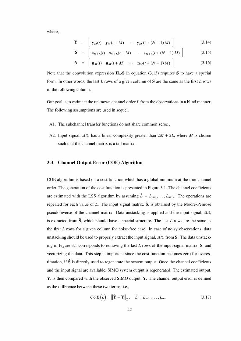
where,

Y =

[yM(t) yM(t + M) · · · yM (t + (N − 1) M)

](3.14)

S =

[sM+L(t) sM+L(t + M) · · · sM+L(t + (N − 1) M)

](3.15)

N =

[nM(t) nM(t + M) · · · nM(t + (N − 1) M)

](3.16)

Note that the convolution expression HMS in equation (3.13) requires S to have a special

form. In other words, the last L rows of a given column of S are the same as the first L rows

of the following column.

Our goal is to estimate the unknown channel order L from the observations in a blind manner.

The following assumptions are used in sequel.

A1. The subchannel transfer functions do not share common zeros .

A2. Input signal, s(t), has a linear complexity greater than 2M + 2L, where M is chosen

such that the channel matrix is a tall matrix.

3.3 Channel Output Error (COE) Algorithm

COE algorithm is based on a cost function which has a global minimum at the true channel

order. The generation of the cost function is presented in Figure 3.1. The channel coefficients

are estimated with the LSS algorithm by assuming L = Lmin, . . . , Lmax. The operations are

repeated for each value of L. The input signal matrix, S, is obtained by the Moore-Penrose

pseudoinverse of the channel matrix. Data unstacking is applied and the input signal, s(t),

is extracted from S, which should have a special structure. The last L rows are the same as

the first L rows for a given column for noise-free case. In case of noisy observations, data

unstacking should be used to properly extract the input signal, s(t), from S. The data unstack-

ing in Figure 3.1 corresponds to removing the last L rows of the input signal matrix, S, and

vectorizing the data. This step is important since the cost function becomes zero for overes-

timation, if S is directly used to regenerate the system output. Once the channel coefficients

and the input signal are available, SIMO system output is regenerated. The estimated output,

Y, is then compared with the observed SIMO output, Y. The channel output error is defined

as the difference between these two terms, i.e.,

COE(L)

=∥∥∥Y − Y

∥∥∥2 , L = Lmin, . . . , Lmax (3.17)

42

The estimated channel order, Lest is found as,

Lest = arg minL

{COE

(L)}

(3.18)

In the following parts, we describe the steps for the proposed method in detail.

.

.

.

( )ˆ ,2ˆ

Lh t

( )ˆ ,1ˆ

Lh t

( )ˆ ,ˆ

L Ph t

( )1y t

( )2y t

( )ˆPy t

.

.

.

( )1y t

( )2y t

( )Py t

( )s t

( ),1Lh t

( ),2Lh t

( ),L Ph t

SY ( )s tData

Stacking

Data

Unstacking

Channel

Estimation

Equalizer

(G)

LSS

Input

Estimation

Data

Stacking

Y

Y

SIMO

ChannelChannel Order estimation: Channel output error

+∑

−

+

+

+

( )1n t

( )2n t

( )pn t

( )ˆCOE L

2.

ˆ

ˆL

h

Figure 3.1: Channel output estimation for channel order L in COE algorithm.

3.3.1 Blind Channel Estimation

LSS algorithm [7, 3] is used to estimate the channel coefficients. LSS is a deterministic

method which uses the isomorphic relation between the input and output signal spaces. An

important property of this algorithm is that it has finite convergence property [7]. Therefore,

it can work with small data packets and gives exact result in noise-free case. We have selected

the LSS algorithm for channel estimation, since it generates common channel zeros, when

the channel order is overestimated. In that case, channel matrix is not full column rank and

COE cost function generates a non-zero value for the overestimation. Lemma-1 describes this

property of the LSS algorithm.

Lemma-1: LSS algorithm [7, 3] generates common channel zeros for noise free case, when

the channel order is overestimated. The remaining zeros are the true channel zeros. If the true

channel order is L and the overestimated channel order is L, the number of common zeros is

L − L.

Proof: The proof is given in Appendix.

Lemma-2 describes the condition of the channel matrix in case of common channel zeros.

43

( )c

h n

,1( )

Lh n

,2( )

Lh n

, ( )L P

h n

( )s n

1( )y n

2ˆ ( )y n

ˆ ( )P

y n

Figure 3.2: Estimated SIMO channel with common channel zeros.

While this is known in the literature, it is presented for the completeness of the discussion.

Lemma-2: If the FIR channels of SIMO system have common zeros, then the channel matrix,

HM whose row size is greater than the column size, is not full column rank.


As a result of Lemma-1, the channel transfer functions estimated by using LSS method in-

clude common zeros besides the true channel zeros, when the channel is overestimated. Then,

the estimated channel is combination of a SIMO channel and a SISO channel, hc(n), whose

zeros are the common zeros as shown in Figure 3.2.

When we want to equalize the channel with the estimated channel coefficients, common chan-

nel transfer function, hc(n), is also equalized with Wiener equalizer besides the true channel.

Wiener equalizer is a linear equalizer and perfect equalization of a FIR modeled SISO channel

is not possible. As a result, channel input cannot be estimated truly when the channel order is

not known.

Another important property of the LSS algorithm is that, the generated common zeros are

located on the unit circle. This property of LSS algorithm is described by Lemma-3, and the

proof is done for the overestimated channel order by one because of the complexity of the

problem. This property is not shared by other blind algorithm, such as SS and CR, which also

generate common zeros. When the common channel zeros are located on the unit circle, the

inverse channel transfer function does not decay to zero as time index go to infinity. Therefore

FIR equalization is not possible. Equalization error is large and increases as the input length

increases due to stability problems. Hence, the error on the estimated channel input due to

44

the equalization of the common channel zeros is higher compared to common zeros located

inside the unit circle.

Lemma-3: When the channel order is overestimated by one, the common zero generated by

the LSS algorithm is located on the unit circle.


In Figure 3.3, pole-zero plots are given for the estimated channels by SS and LSS, when

the channel order is overestimated. The true channel order is L = 3 and the number of

subchannels is P = 2. Channel order is taken as L = 6 in SS and LSS algorithms. As shown

in Figure 3.3, common channel zeros are generated by both of the algorithms. However,

common zeros in LSS are close to the unit circle. Therefore, this gives a good idea about

the performance of the LSS algorithm when it is used within the proposed channel order

estimation methods. Since the equalization of channels with zeros on unit circle is harder,

equalization error is higher for LSS case when the channel order is overestimated.

45

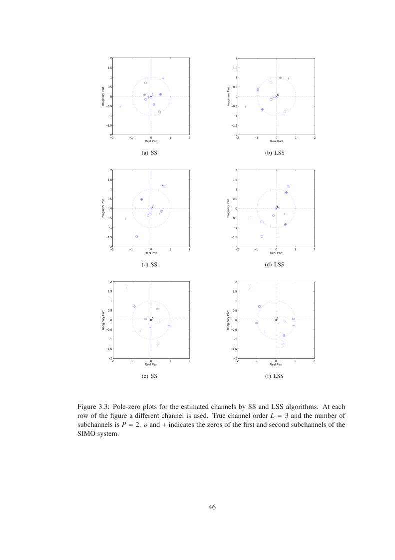
−2 −1 0 1 2−2

−1.5

−1

−0.5

0

0.5

1

1.5

2

6

Real Part

Imag

inar

y P

art

(a) SS

−2 −1 0 1 2−2

−1.5

−1

−0.5

0

0.5

1

1.5

2

6

Real Part

Imag

inar

y P

art

(b) LSS

−2 −1 0 1 2−2

−1.5

−1

−0.5

0

0.5

1

1.5

2

6

Real Part

Imag

inar

y P

art

(c) SS

−2 −1 0 1 2−2

−1.5

−1

−0.5

0

0.5

1

1.5

2

6

Real Part

Imag

inar

y P

art

(d) LSS

−2 −1 0 1 2−2

−1.5

−1

−0.5

0

0.5

1

1.5

2

6

Real Part

Imag

inar

y P

art

(e) SS

−2 −1 0 1 2−2

−1.5

−1

−0.5

0

0.5

1

1.5

2

6

Real Part

Imag

inar

y P

art

(f) LSS

Figure 3.3: Pole-zero plots for the estimated channels by SS and LSS algorithms. At eachrow of the figure a different channel is used. True channel order L = 3 and the number ofsubchannels is P = 2. o and + indicates the zeros of the first and second subchannels of theSIMO system.

46

3.3.2 Channel Equalization and Input Estimation

Once the channel coefficients are available, the input signal for the SIMO system can be

obtained by using Moore-Penrose pseudoinverse of the channel matrix. The input signal

matrix, S, is obtained as S = GY, where G is the pseudoinverse of HM , G = H†M . Note

that the pseudoinverse can be found even when HM is not full column rank. In that case,

pseudoinverse uses singular value decomposition and singular values below a certain level

are taken as zero for the inverse operation [35]. (Built in pseudoinverse function in MATLAB

is directly used. Default threshold value defined in the Matlab function is used.)

3.3.3 Data Unstacking

For noise free case, SIMO system output can be obtained through a convolution operation

which can be written as a matrix equation given below,

Y = HMS (3.19)

This equation represents a true convolution operation only if the input signal data matrix, S,

is constructed appropriately as explained after the equation (3.13). When there is noise in the

observations and S is estimated by the pseudoinverse of the channel matrix as S = H†MY, the

structure of the S matrix is not preserved in S. Data unstacking is used to obtain the input

signal, s(t) from S appropriately. Then a new input signal data matrix which has the similar

structure like S can be constructed from s(t), or s(t) can be directly used in the convolution

operation as shown in Figure 3.1. Note that, if data unstacking is not performed and S is

directly used to generate an estimate of the channel output, Y = HMS, COE becomes zero

independent of the value of the overestimated channel order, L, for noise free case. Therefore

data unstacking results nonzero COE for overestimation and we obtain a ”convex-like” cost

function for the channel order estimation. Data unstacking deletes the last L rows of S and

s(t) is obtained from this matrix through a vectorization operation. A toy example for data

unstacking is given below for L = 2.

47

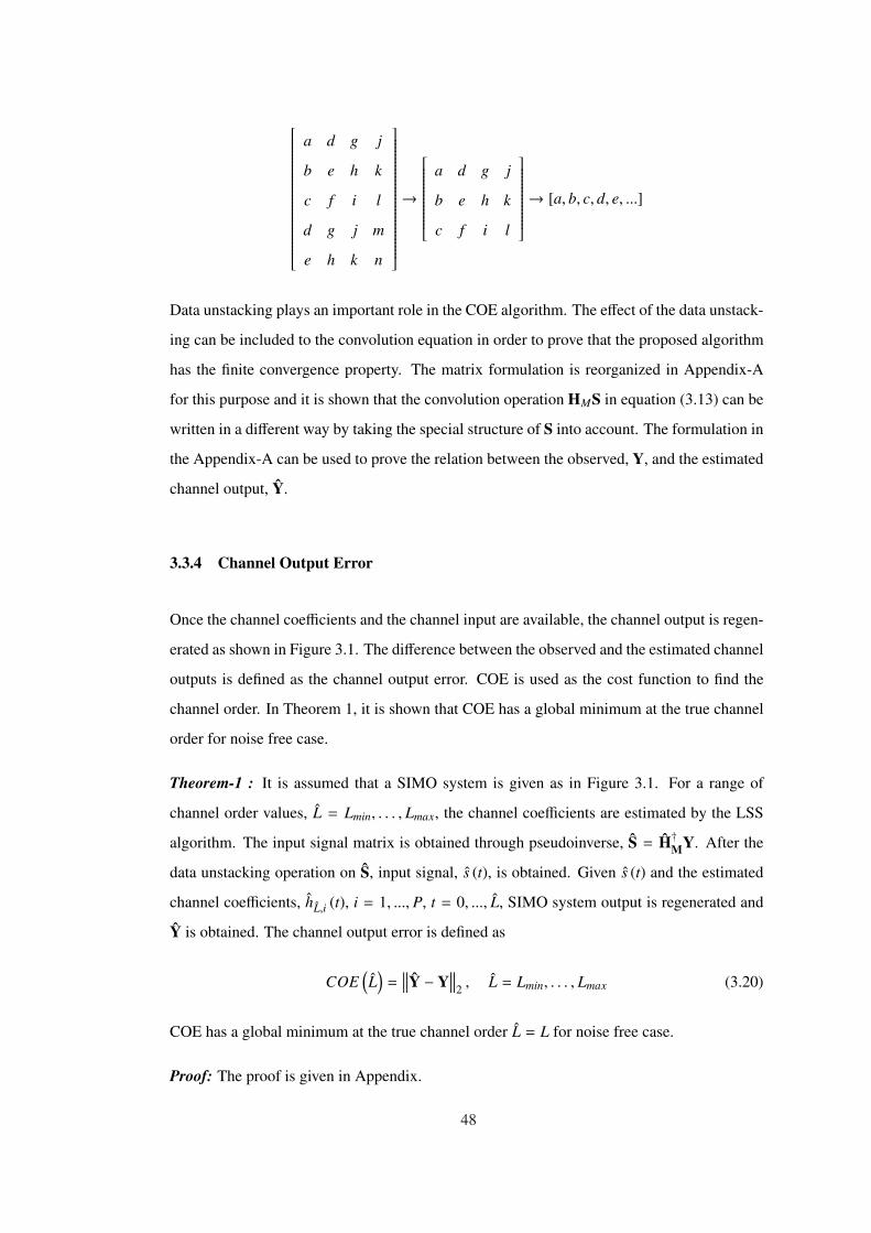
a d g j

b e h k

c f i l

d g j m

e h k n

→

a d g j

b e h k

c f i l

→ [a, b, c, d, e, ...]

Data unstacking plays an important role in the COE algorithm. The effect of the data unstack-

ing can be included to the convolution equation in order to prove that the proposed algorithm

has the finite convergence property. The matrix formulation is reorganized in Appendix-A

for this purpose and it is shown that the convolution operation HMS in equation (3.13) can be

written in a different way by taking the special structure of S into account. The formulation in

the Appendix-A can be used to prove the relation between the observed, Y, and the estimated

channel output, Y.

3.3.4 Channel Output Error

Once the channel coefficients and the channel input are available, the channel output is regen-

erated as shown in Figure 3.1. The difference between the observed and the estimated channel

outputs is defined as the channel output error. COE is used as the cost function to find the

channel order. In Theorem 1, it is shown that COE has a global minimum at the true channel

order for noise free case.

Theorem-1 : It is assumed that a SIMO system is given as in Figure 3.1. For a range of

channel order values, L = Lmin, . . . , Lmax, the channel coefficients are estimated by the LSS

algorithm. The input signal matrix is obtained through pseudoinverse, S = H†MY. After the

data unstacking operation on S, input signal, s (t), is obtained. Given s (t) and the estimated

channel coefficients, hL,i (t), i = 1, ..., P, t = 0, ..., L, SIMO system output is regenerated and

Y is obtained. The channel output error is defined as

COE(L)

=∥∥∥Y − Y

∥∥∥2 , L = Lmin, . . . , Lmax (3.20)

COE has a global minimum at the true channel order L = L for noise free case.


48

In Figure 3.4, Theorem-1 is verified for noisy observations through simulations. Channel

order is selected as L = 5 and the number of channels is P = 3. Channel coefficients are

complex values chosen randomly from a zero mean unit variance Gaussian set and change in

each trial. For different values of channel orders, COE is computed for 200 trials and average

of the COE’s are taken as the final COE for a given channel order. The results also include the

wrong channel order estimation cases, that is outliers are not discarded. As shown in Figure

3.4, COE has a global minimum at the true channel order, L = 5.

1 2 3 4 5 6 7 8 9−26

−24

−22

−20

−18

−16

−14

−12

−10

−8

−6

Channel order

CO

E, d

B

SNR = 10dBSNR = 20dBSNR = 30dB

Figure 3.4: Channel output error (COE) for noisy observations.

3.4 Channel Matrix Recursion Algorithm (CMR) Algorithm

Channel matrix recursion algorithm is based on the estimation channel matrix via LSS algo-

rithm for different channel orders. Before the explanation of the algorithm details, it is better

to summarize some important properties of the LSS algorithm for noise free case.

• When the channel order is overestimated, LSS results common zeros besides the true

channel zeros.

• When the channel order is overestimated, the estimated channel matrix is not full col-

umn rank as a result of common zeros.

Properties of the LSS algorithm given above are stated by Lemma-1 and Lemma-2 in thischapter.

49

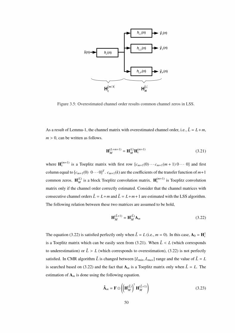
( )c

h n

,1( )

Lh n

,2( )

Lh n

, ( )L P

h n

( )s n

1( )y n

2ˆ ( )y n

ˆ ( )P

y n

( )LM

H( )1m

c

+H

Figure 3.5: Overestimated channel order results common channel zeros in LSS.

As a result of Lemma-1, the channel matrix with overestimated channel order, i.e., L = L + m,

m > 0, can be written as follows.

H(L+m+1)M = H(L)

M H(m+1)c (3.21)

where H(m+1)c is a Toeplitz matrix with first row [cm+1(0) · · · cm+1(m + 1) 0 · · · 0] and first

column equal to [cm+1(0) 0 · · · 0]T . cm+1(k) are the coefficients of the transfer function of m+1

common zeros. H(L)M is a block Toeplitz convolution matrix. H(m+1)

c is Toeplitz convolution

matrix only if the channel order correctly estimated. Consider that the channel matrices with

consecutive channel orders L = L+m and L = L+m+1 are estimated with the LSS algorithm.

The following relation between these two matrices are assumed to be hold,

H(L+1)M = H(L)

M Am (3.22)

The equation (3.22) is satisfied perfectly only when L = L (i.e., m = 0). In this case, A0 = H1c

is a Toeplitz matrix which can be easily seen from (3.21). When L < L (which corresponds

to underestimation) or L > L (which corresponds to overestimation), (3.22) is not perfectly

satisfied. In CMR algorithm L is changed between [Lmin, Lmax] range and the value of L = L

is searched based on (3.22) and the fact that Am is a Toeplitz matrix only when L = L. The

estimation of Am is done using the following equation.

Am = F �((

H(L)M

)†H(L+1)

M

)(3.23)

50

where, � is the Hadamard product and (M + L + m) × (M + L + m + 1) matrix F is a Toeplitz

matrix with first row equal to [1 1 0 · · · 0] and first column equal to [1 0 · · · 0]T . (.)† indi-

cates the Moore-Penrose pseudoinverse. There are two functions of F in (3.22). The first one

is a filtering action which selects the diagonals from the matrix in parenthesis to generate the

expected matrix structure in (3.22) for m = 0. The second is to generate error for overestima-

tion. In the following theorem, CMR cost function is defined and its main characteristics are

described.

Theorem-2 : It is assumed that a SIMO system is given as in Figure 3.1. For a range of

channel order values, L = L + m = Lmin, · · · , Lmax, the channel coefficients are estimated by

the LSS algorithm. Let the estimated channel matrix is given by HLM for the channel order L.

M is chosen such that the channel matrix is a tall matrix. The cost function is defined as,

ECMR(L)

=∥∥∥∥H(L+1)

M −H(L)M Am

∥∥∥∥2/∥∥∥∥H(L+1)

M

∥∥∥∥2

(3.24)

Am = F � Bm (3.25)

Bm =(H(L+m)

M

)†H(L+m+1)

M (3.26)

has global minimum at true channel order, L = L, in the noise free case.

Proof : The proof is given at the Appendix.

In Figure 3.6, Theorem-2 is verified for noisy observations through simulations. Channel

order is selected as L = 5 and the number of channels is P = 3. Channel coefficients are

complex values chosen randomly from a zero mean unit variance Gaussian set and change in

each trial. For different values of the channel orders, ECMR is calculated for 200 trials and

average of the ECMR’s are taken as the final ECMR for a given channel order. The results also

include the wrong channel order estimation cases. As shown in Figure 3.6, CMR has a global

minimum at the true channel order, L = 5.

51

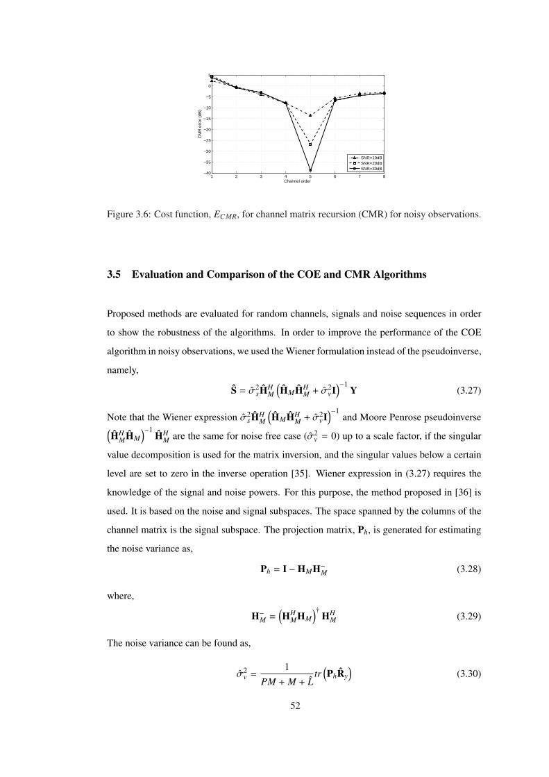
1 2 3 4 5 6 7 8−40

−35

−30

−25

−20

−15

−10

−5

0

5

Channel order

CM

R e

rror

(dB

)

SNR=10dBSNR=20dBSNR=30dB

Figure 3.6: Cost function, ECMR, for channel matrix recursion (CMR) for noisy observations.

3.5 Evaluation and Comparison of the COE and CMR Algorithms

Proposed methods are evaluated for random channels, signals and noise sequences in order

to show the robustness of the algorithms. In order to improve the performance of the COE

algorithm in noisy observations, we used the Wiener formulation instead of the pseudoinverse,

namely,

S = σ2sHH

M

(HMHH

M + σ2vI

)−1Y (3.27)

Note that the Wiener expression σ2sHH

M

(HMHH

M + σ2vI

)−1and Moore Penrose pseudoinverse

(HH

MHM)−1

HHM are the same for noise free case (σ2

v = 0) up to a scale factor, if the singular

value decomposition is used for the matrix inversion, and the singular values below a certain

level are set to zero in the inverse operation [35]. Wiener expression in (3.27) requires the

knowledge of the signal and noise powers. For this purpose, the method proposed in [36] is

used. It is based on the noise and signal subspaces. The space spanned by the columns of the

channel matrix is the signal subspace. The projection matrix, Ph, is generated for estimating

the noise variance as,

Ph = I −HMH−M (3.28)

where,

H−M =(HH

MHM)†

HHM (3.29)

The noise variance can be found as,

σ2v =

1PM + M + L

tr(PhRy

)(3.30)

52

where Ry = 1MP YYH . Signal power is found by removing the noise part from the output

correlation matrix, Ry, i.e.,

Rs = H−M(Ry − σ2

vI) (

H−M)H

(3.31)

σ2s = tr

(Rs

)/(M + L

)(3.32)

The SNR for the evaluation of the algorithms is is computed as,

S NR =1

Pσ2 E

P∑

j=1

∣∣∣y j (k)∣∣∣2 (3.33)

where P is the number of outputs, σ2 is the noise variance and y j (k) is the noiseless samples

of the jth output.

In the simulations, complex channel coefficients are selected from a zero mean unit variance

Gaussian distribution. Input is a QPSK modulated sequence with 100 samples and 200 trials

are performed to report the average of these trials. The value of M in (3.8) is chosen as M = L.

Figure 3.7 shows the approximate probability density functions (pdf) of different channel

order estimation algorithms and the proposed methods for a S NR = 15dB. COE and CMR

give the best distribution in terms of finding the true channel order. COE and CMR have

small underestimate tails but they do not have overestimation. MDL has both underestimate

and overestimate tails but it has the second best characteristics after COE and CMR. ID+EQ

has a significant tendency for underestimation. AIC has a strong overestimation characteristic

mostly missing the true channel order due to the fact that it works properly only at high SNR

(S NR > 25dB). Liavas also works properly at high SNR and its distribution is not satisfactory

for low SNR.

Table 3.1 and Table 3.2 summarize the performance of COE, CMR, MDL and AIC algo-

rithms for different number of channels and channel orders. The robustness of the proposed

algorithms for different SIMO parameters can be seen easily. For COE and CMR algorithms,

estimation performance is improved as the number of channels increases. Performance de-

creases as the channel order is increased. Overall, COE and CMR algorithms return the best

performance almost all of the cases considered in the tables. CMR shows a better performance

than COE when the channel order (L < 5) and the number of channels is small (P < 5). COE

is the best algorithm when the channel order and number of channels is large. There is a small

part (L > 7, P > 4) where MDL seems to perform better than CMR. If the number of samples

53

for the input signal is increased to 150 samples, the performance of CMR increases. As a

result, it becomes better than MDL for all cases. In this case, COE is better than CMR when

L > 7 and P > 2. Therefore, the increase in number of samples has more positive effect for

the CMR algorithm. However further increase do not change the performance significantly.

Liavas algorithm has the same tendency as the COE. In other words, its performance increases

with the number of channels and it decreases as the channel order is increased. AIC and MDL

show somehow mixed and opposite characteristics. While AIC performance has a tendency

to fall as the number of channels increases, MDL performance mostly improves except for

L = 2.

The probability of correct channel order estimation is presented in Figures 3.8, 3.9 and 3.10

for (L = 3, P = 3); (L = 5, P = 3) and (L = 5, P = 5) respectively. As shown in these figures,

the proposed algorithms outperform the alternatives in all SNR ranges. The characteristics of

the algorithms observed in Table 3.1 and 3.2 are also verified for different SNR values in these

figures. CMR is the best one when the channel order and the number of channels is small. As

the channel order or the number of channels increases, the performance of the COE algorithm

gets better than the CMR approximately after S NR > 6dB.

3.6 Conclusion

Two new channel order estimation algorithms, COE and CMR are proposed for FIR SIMO

systems. Both of these algorithms are based on the LSS algorithm which generates common

channel zeros for the overestimated channel order. In COE, channel coefficients and the input

signal are estimated to regenerate the SIMO system output in order to compare it with the

observed output. It is shown that COE has a global minimum at the true channel order for

noise free case. CMR uses the relation between the channel matrices for the overestimated

channel orders. It also finds the true channel order for the noise free case. CMR is a compu-

tationally efficient alternative to the COE algorithm. It performs better than COE algorithm

especially when the number of channels and channel order is small. Both COE and CMR

perform significantly better than the alternative algorithms for a variety of cases.

54

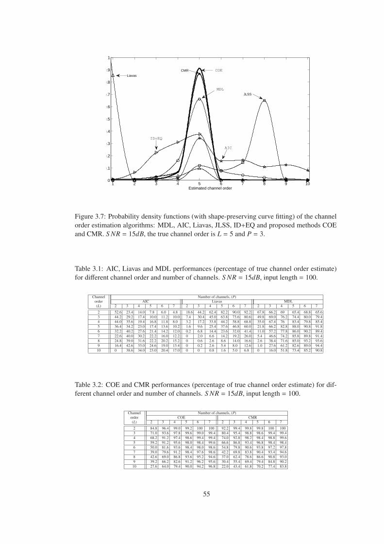
1 2 3 4 5 6 7 8 9 100

0.1

0.2

0.3

0.4

0.5

0.6

0.7

0.8

0.9

1

Estimated channel order

ID+EQ

JLSS

MDL

AIC

Liavas

CMR COE

Figure 3.7: Probability density functions (with shape-preserving curve fitting) of the channelorder estimation algorithms: MDL, AIC, Liavas, JLSS, ID+EQ and proposed methods COEand CMR. S NR = 15dB, the true channel order is L = 5 and P = 3.

Table 3.1: AIC, Liavas and MDL performances (percentage of true channel order estimate)for different channel order and number of channels. S NR = 15dB, input length = 100.

Channel Number of channels, (P)order AIC Liavas MDL(L) 2 3 4 5 6 7 2 3 4 5 6 7 2 3 4 5 6 7

2 52.6 23.4 14.0 7.8 6.0 4.8 18.6 44.2 62.4 82.2 90.0 92.2 67.8 66.2 69 65.4 68.8 65.63 44.2 29.2 17.4 10.0 11.2 10.0 7.4 30.4 45.0 63.8 73.6 80.6 49.8 69.0 76.2 74.4 80.0 79.44 44.0 35.6 19.4 16.8 11.8 8.0 3.2 17.2 33.8 44.2 58.8 68.8 35.0 67.4 76 83.4 79.8 85.45 36.4 34.2 23.0 17.4 13.6 10.2 1.6 9.6 25.4 37.6 46.8 60.0 21.8 66.2 82.8 88.0 90.8 91.86 32.2 40.2 27.6 21.4 14.2 12.0 0.2 6.8 14.4 23.6 32.0 41.4 11.0 57.2 77.8 86.0 90.2 89.47 22.6 40.0 30.2 22.2 16.0 12.2 0 2.0 6.6 14.2 19.2 26.0 5.4 46.6 74.2 85.8 89.8 91.48 24.8 39.0 31.6 22.2 20.2 15.2 0 0.6 2.6 8.6 14.0 16.6 2.6 38.4 71.6 85.0 93.2 93.69 16.4 42.6 33.0 24.6 19.0 13.4 0 0.2 2.6 5.4 8.0 12.6 1.0 27.6 61.2 82.6 89.0 94.4

10 0 38.6 34.0 23.0 20.4 17.0 0 0 0.8 1.6 5.0 6.8 0 16.0 51.8 73.4 85.2 90.8

Table 3.2: COE and CMR performances (percentage of true channel order estimate) for dif-ferent channel order and number of channels. S NR = 15dB, input length = 100.

Channel Number of channels, (P)order COE CMR(L) 2 3 4 5 6 7 2 3 4 5 6 7

2 84.8 96.4 99.0 99.2 100 100 92.2 99.4 99.8 99.8 100 1003 71.0 93.6 97.8 99.6 99.0 99.4 80.4 95.4 98.8 98.6 99.4 99.44 68.2 91.2 97.4 98.6 99.4 99.4 74.0 92.8 98.2 98.4 98.8 99.65 59.2 91.2 95.6 98.0 98.4 99.6 66.6 86.8 93.4 96.8 98.4 98.46 50.0 81.6 93.6 98.4 98.0 98.6 54.8 79.8 90.6 93.8 97.2 97.87 39.0 79.6 91.2 98.4 97.6 98.6 42.2 69.8 83.8 90.4 93.4 94.68 42.6 69.0 86.8 93.6 95.2 94.6 37.0 62.4 78.6 86.6 90.8 93.09 39.2 66.2 82.6 91.2 96.2 95.6 30.4 55.4 69.4 79.4 84.8 90.210 27.6 64.0 79.4 90.0 94.2 96.8 22.0 43.4 61.8 70.2 77.4 83.8

55

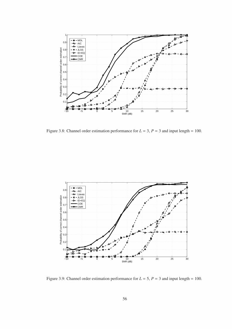
−10 −5 0 5 10 15 20 25 300

0.1

0.2

0.3

0.4

0.5

0.6

0.7

0.8

0.9

1

SNR (dB)

Pro

babi

lity

of c

orre

ct c

hann

el o

rder

est

imat

ion

MDLAICLiavasJLSSID+EQCOECMR

Figure 3.8: Channel order estimation performance for L = 3, P = 3 and input length = 100.

−10 −5 0 5 10 15 20 25 300

0.1

0.2

0.3

0.4

0.5

0.6

0.7

0.8

0.9

1

SNR (dB)

Pro

babi

lity

of c

orre

ct c

hann

el o

rder

est

imat

ion



56

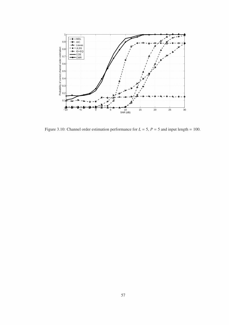
−10 −5 0 5 10 15 20 25 300

0.1

0.2

0.3

0.4

0.5

0.6

0.7

0.8

0.9

1

SNR (dB)

Pro

babi

lity

of c

orre

ct c

hann

el o

rder

est

imat

ion



57

CHAPTER 4

CHANNEL ORDER ESTIMATION USING TRAINING DATA

4.1 Introduction

In this chapter, channel order estimation is considered for the systems which uses training se-

quences. The motivation here is to understand and compare the order estimation performance

with the blind techniques. Blind methods do not use training data to identify/ equalize the

channel. Therefore they are more bandwidth efficient methods. Blind methods are preferred

for the systems which have synchronization problem, because they do not have to synchronize

to the training data for channel identification. On the other hand,blind methods can identify

the channel up to a scale factor for SIMO systems, while the training based methods can

identify the channel exactly.

Training based methods estimate channel coefficients using only the received data containing

the known symbols. All other observations are ignored. Therefore synchronization should

be achieved for channel identification. Otherwise, expected performance cannot be obtained.

Synchronization should be achieved before the equalization or jointly with the channel iden-

tification, since the channel coefficients cannot be found without knowing the placement of

the known symbols at received signal. In [34], synchronization and channel identification is

achieved in a joint manner using a single cost function which has a global minimum.

Another problem to be solved in training based methods is the channel order estimation as in

the case of blind methods. In training based methods, channel order is usually assumed to be

known as in [34] or they use overestimated channel order employing algorithms like MDL

and AIC. The robustness of training based methods for overestimated channel order is low at

low SNR.

58

The bit error rate (BER) performance of the training based methods is better than the blind

methods when the synchronization is achieved and the channel order is known. However if

one of them is not properly estimated, their performance decreases and even becomes worse

than the blind methods. The performance of blind methods can be increased by using training

data beside the unknown data. This can also be thought from the side of training based

methods. With the help of blind methods, which enable the use of whole received data, it is

possible to obtain the same performance with smaller number of training data. This type of

methods are called as the semi-blind methods and have better performance than the training

only and blind only methods.

To our knowledge, there is no algorithm proposed for channel order estimation using only the

training data or using the benefit of training data in channel order estimation. In this chapter,

two new channel order estimation algorithms namely Channel Input Error with Semiblind

Channel Estimator (CIES) and Channel Input Error with Blind Channel Estimator (CIEB) are

proposed. They use the training data to obtain the channel order. In both of the algorithms,

channel input error, which is the difference between the estimated and known pilot symbols,

is used as the cost function to obtain the true channel order. The difference between CIEB

and CIES is due to the method used in channel estimation. In CIEB, channel is estimated

with LSS algorithm in a blind manner. In CIES, channel is estimated by means of a semi

blind method, which is proposed in this thesis. CIES is obtained by the modification of

the method [38] which combines SS and least squares fit on training sequence (LST) in a

single cost function to obtain the channel coefficients. In the modification, LSS algorithm

is used instead of the SS algorithm. In this way, a better algorithm is obtained in terms

estimating the channel order in noisy observations. This is due to the fact that when the

channel is estimated by LSS with overestimated channel order, common zeros produced by

the LSS algorithm are placed on unit circle. This leads to high error in the equalization

step of CIES and generates deeper valleys at true channel order. Both of the algorithms

require synchronization to find the location of training symbols. In CIES, synchronization and

channel order estimation is achieved in a joint manner with multidimensional search for the

channel order and synchronization point. Therefore it has high computational complexity. In

CIEB, synchronization is achieved after channel equalization and on the ISI removed signal by

using the optimum synchronization method proposed in [39]. Proposed algorithms CIES and

CIEB are compared with blind channel order estimation algorithms in estimating the channel

59

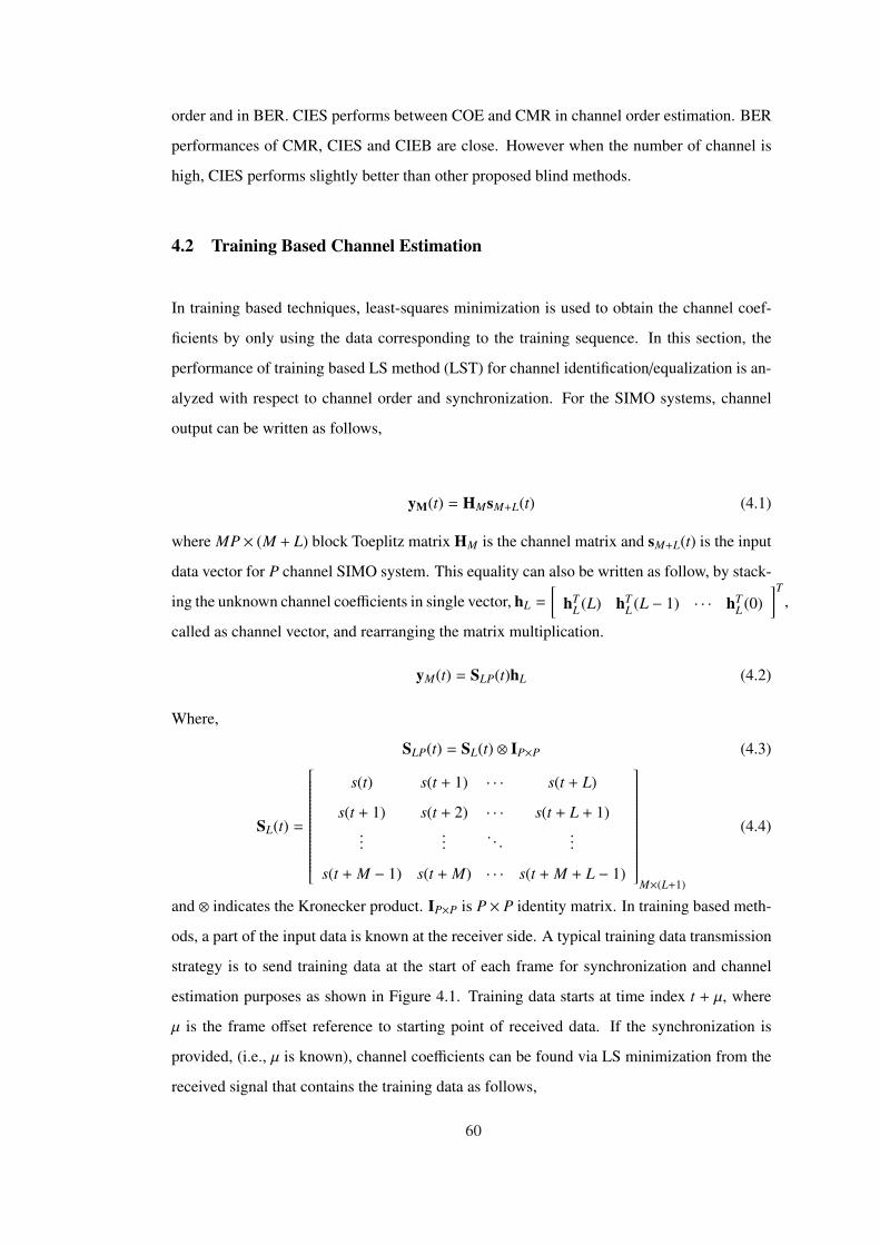
order and in BER. CIES performs between COE and CMR in channel order estimation. BER

performances of CMR, CIES and CIEB are close. However when the number of channel is

high, CIES performs slightly better than other proposed blind methods.

4.2 Training Based Channel Estimation

In training based techniques, least-squares minimization is used to obtain the channel coef-

ficients by only using the data corresponding to the training sequence. In this section, the

performance of training based LS method (LST) for channel identification/equalization is an-

alyzed with respect to channel order and synchronization. For the SIMO systems, channel

output can be written as follows,

yM(t) = HMsM+L(t) (4.1)

where MP × (M + L) block Toeplitz matrix HM is the channel matrix and sM+L(t) is the input

data vector for P channel SIMO system. This equality can also be written as follow, by stack-

ing the unknown channel coefficients in single vector, hL =

[hT

L (L) hTL (L − 1) · · · hT

L (0)]T

,

called as channel vector, and rearranging the matrix multiplication.

yM(t) = SLP(t)hL (4.2)

Where,

SLP(t) = SL(t) ⊗ IP×P (4.3)

SL(t) =

s(t) s(t + 1) · · · s(t + L)

s(t + 1) s(t + 2) · · · s(t + L + 1)...

.... . .

...

s(t + M − 1) s(t + M) · · · s(t + M + L − 1)

M×(L+1)

(4.4)

and ⊗ indicates the Kronecker product. IP×P is P × P identity matrix. In training based meth-

ods, a part of the input data is known at the receiver side. A typical training data transmission

strategy is to send training data at the start of each frame for synchronization and channel

estimation purposes as shown in Figure 4.1. Training data starts at time index t + µ, where

µ is the frame offset reference to starting point of received data. If the synchronization is

provided, (i.e., µ is known), channel coefficients can be found via LS minimization from the

received signal that contains the training data as follows,

60

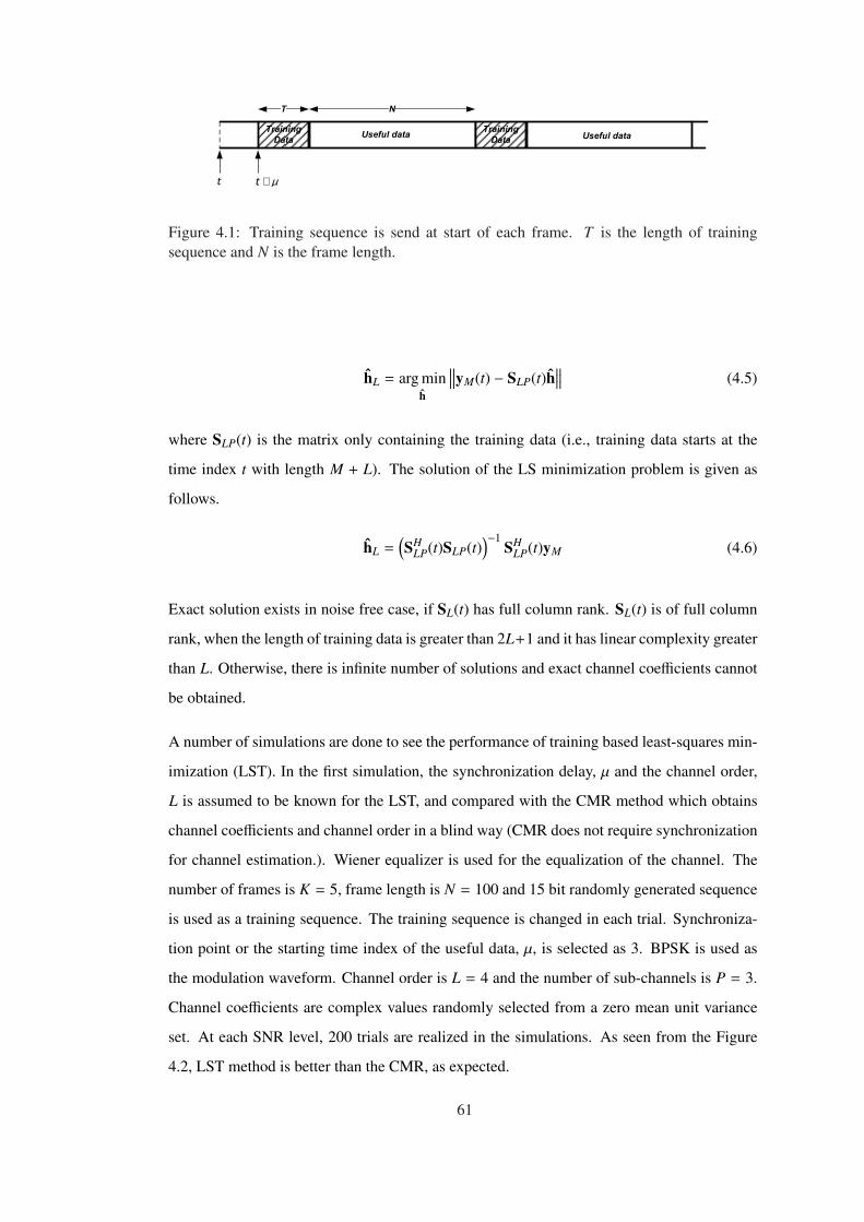
Training

DataUseful data

t µ+

Training

Data

T N

t

Useful data

Figure 4.1: Training sequence is send at start of each frame. T is the length of trainingsequence and N is the frame length.

hL = arg minh

∥∥∥yM(t) − SLP(t)h∥∥∥ (4.5)

where SLP(t) is the matrix only containing the training data (i.e., training data starts at the

time index t with length M + L). The solution of the LS minimization problem is given as

follows.

hL =(SH

LP(t)SLP(t))−1

SHLP(t)yM (4.6)

Exact solution exists in noise free case, if SL(t) has full column rank. SL(t) is of full column

rank, when the length of training data is greater than 2L+1 and it has linear complexity greater

than L. Otherwise, there is infinite number of solutions and exact channel coefficients cannot

be obtained.

A number of simulations are done to see the performance of training based least-squares min-

imization (LST). In the first simulation, the synchronization delay, µ and the channel order,

L is assumed to be known for the LST, and compared with the CMR method which obtains

channel coefficients and channel order in a blind way (CMR does not require synchronization

for channel estimation.). Wiener equalizer is used for the equalization of the channel. The

number of frames is K = 5, frame length is N = 100 and 15 bit randomly generated sequence

is used as a training sequence. The training sequence is changed in each trial. Synchroniza-

tion point or the starting time index of the useful data, µ, is selected as 3. BPSK is used as

the modulation waveform. Channel order is L = 4 and the number of sub-channels is P = 3.

Channel coefficients are complex values randomly selected from a zero mean unit variance

set. At each SNR level, 200 trials are realized in the simulations. As seen from the Figure

4.2, LST method is better than the CMR, as expected.

61

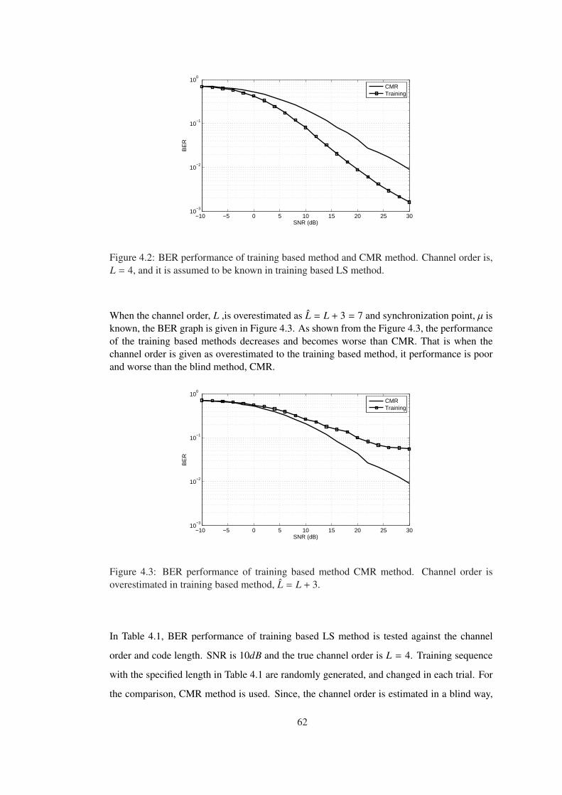
−10 −5 0 5 10 15 20 25 3010

−3

10−2

10−1

100

SNR (dB)

BE

R

CMRTraining

Figure 4.2: BER performance of training based method and CMR method. Channel order is,L = 4, and it is assumed to be known in training based LS method.

When the channel order, L ,is overestimated as L = L + 3 = 7 and synchronization point, µ isknown, the BER graph is given in Figure 4.3. As shown from the Figure 4.3, the performanceof the training based methods decreases and becomes worse than CMR. That is when thechannel order is given as overestimated to the training based method, it performance is poorand worse than the blind method, CMR.

−10 −5 0 5 10 15 20 25 3010

−3

10−2

10−1

100

SNR (dB)

BE

R

CMRTraining

Figure 4.3: BER performance of training based method CMR method. Channel order isoverestimated in training based method, L = L + 3.

In Table 4.1, BER performance of training based LS method is tested against the channel

order and code length. SNR is 10dB and the true channel order is L = 4. Training sequence

with the specified length in Table 4.1 are randomly generated, and changed in each trial. For

the comparison, CMR method is used. Since, the channel order is estimated in a blind way,

62

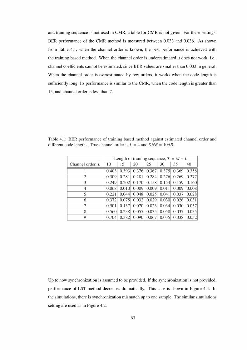
and training sequence is not used in CMR, a table for CMR is not given. For these settings,

BER performance of the CMR method is measured between 0.033 and 0.036. As shown

from Table 4.1, when the channel order is known, the best performance is achieved with

the training based method. When the channel order is underestimated it does not work, i.e.,

channel coefficients cannot be estimated, since BER values are smaller than 0.033 in general.

When the channel order is overestimated by few orders, it works when the code length is

sufficiently long. Its performance is similar to the CMR, when the code length is greater than

15, and channel order is less than 7.

Table 4.1: BER performance of training based method against estimated channel order anddifferent code lengths. True channel order is L = 4 and S NR = 10dB.

Length of training sequence, T = M + LChannel order, L 10 15 20 25 30 35 40

1 0.403 0.393 0.376 0.367 0.375 0.369 0.3582 0.309 0.281 0.281 0.284 0.276 0.269 0.2773 0.249 0.202 0.170 0.158 0.154 0.159 0.1604 0.068 0.010 0.009 0.009 0.011 0.009 0.0085 0.221 0.044 0.048 0.025 0.041 0.037 0.0286 0.372 0.075 0.032 0.029 0.030 0.026 0.0317 0.501 0.137 0.070 0.023 0.034 0.030 0.0578 0.560 0.238 0.055 0.035 0.058 0.037 0.0359 0.704 0.382 0.090 0.067 0.035 0.038 0.052

Up to now synchronization is assumed to be provided. If the synchronization is not provided,

performance of LST method decreases dramatically. This case is shown in Figure 4.4. In

the simulations, there is synchronization mismatch up to one sample. The similar simulations

setting are used as in Figure 4.2.

63

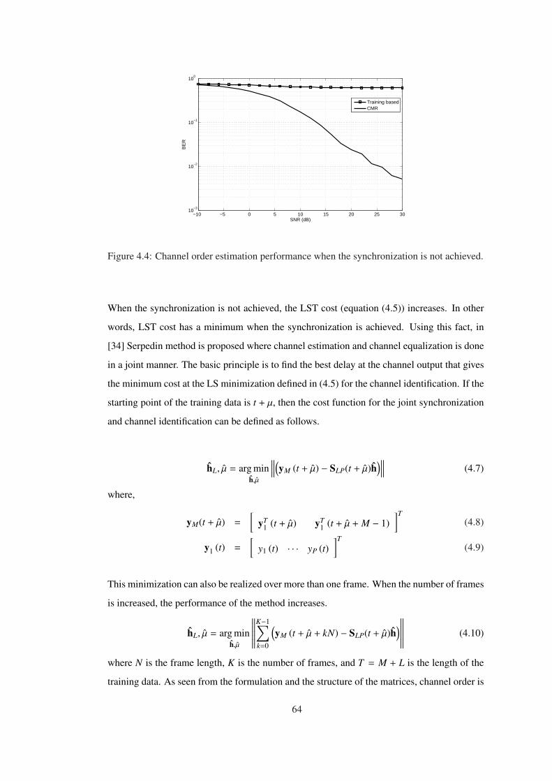
−10 −5 0 5 10 15 20 25 3010

−3

10−2

10−1

100

SNR (dB)

BE

R

Training basedCMR

Figure 4.4: Channel order estimation performance when the synchronization is not achieved.

When the synchronization is not achieved, the LST cost (equation (4.5)) increases. In other

words, LST cost has a minimum when the synchronization is achieved. Using this fact, in

[34] Serpedin method is proposed where channel estimation and channel equalization is done

in a joint manner. The basic principle is to find the best delay at the channel output that gives

the minimum cost at the LS minimization defined in (4.5) for the channel identification. If the

starting point of the training data is t + µ, then the cost function for the joint synchronization

and channel identification can be defined as follows.

hL, µ = arg minh,µ

∥∥∥∥(yM (t + µ) − SLP(t + µ)h

)∥∥∥∥ (4.7)

where,

yM(t + µ) =

[yT

1 (t + µ) yT1 (t + µ + M − 1)

]T(4.8)

y1 (t) =

[y1 (t) · · · yP (t)

]T(4.9)

This minimization can also be realized over more than one frame. When the number of frames

is increased, the performance of the method increases.

hL, µ = arg minh,µ

∥∥∥∥∥∥∥K−1∑

k=0

(yM (t + µ + kN) − SLP(t + µ)h

)∥∥∥∥∥∥∥ (4.10)

where N is the frame length, K is the number of frames, and T = M + L is the length of the

training data. As seen from the formulation and the structure of the matrices, channel order is

64

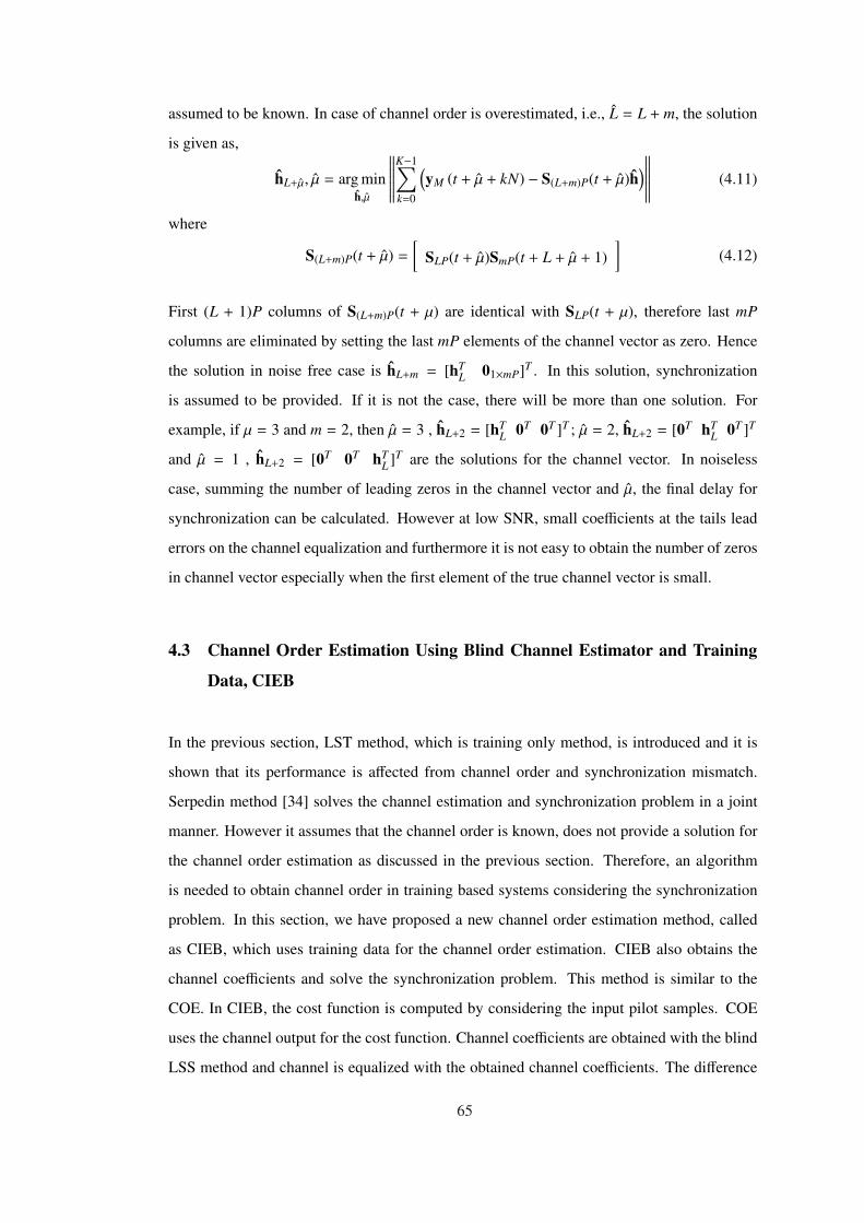
assumed to be known. In case of channel order is overestimated, i.e., L = L + m, the solution

is given as,

hL+µ, µ = arg minh,µ

∥∥∥∥∥∥∥K−1∑

k=0

(yM (t + µ + kN) − S(L+m)P(t + µ)h

)∥∥∥∥∥∥∥ (4.11)

where

S(L+m)P(t + µ) =

[SLP(t + µ)SmP(t + L + µ + 1)

](4.12)

First (L + 1)P columns of S(L+m)P(t + µ) are identical with SLP(t + µ), therefore last mP

columns are eliminated by setting the last mP elements of the channel vector as zero. Hence

the solution in noise free case is hL+m = [hTL 01×mP]T . In this solution, synchronization

is assumed to be provided. If it is not the case, there will be more than one solution. For

example, if µ = 3 and m = 2, then µ = 3 , hL+2 = [hTL 0T 0T ]T ; µ = 2, hL+2 = [0T hT

L 0T ]T

and µ = 1 , hL+2 = [0T 0T hTL ]T are the solutions for the channel vector. In noiseless

case, summing the number of leading zeros in the channel vector and µ, the final delay for

synchronization can be calculated. However at low SNR, small coefficients at the tails lead

errors on the channel equalization and furthermore it is not easy to obtain the number of zeros

in channel vector especially when the first element of the true channel vector is small.

4.3 Channel Order Estimation Using Blind Channel Estimator and Training

Data, CIEB

In the previous section, LST method, which is training only method, is introduced and it is

shown that its performance is affected from channel order and synchronization mismatch.

Serpedin method [34] solves the channel estimation and synchronization problem in a joint

manner. However it assumes that the channel order is known, does not provide a solution for

the channel order estimation as discussed in the previous section. Therefore, an algorithm

is needed to obtain channel order in training based systems considering the synchronization

problem. In this section, we have proposed a new channel order estimation method, called

as CIEB, which uses training data for the channel order estimation. CIEB also obtains the

channel coefficients and solve the synchronization problem. This method is similar to the

COE. In CIEB, the cost function is computed by considering the input pilot samples. COE

uses the channel output for the cost function. Channel coefficients are obtained with the blind

LSS method and channel is equalized with the obtained channel coefficients. The difference

65

.

.

.

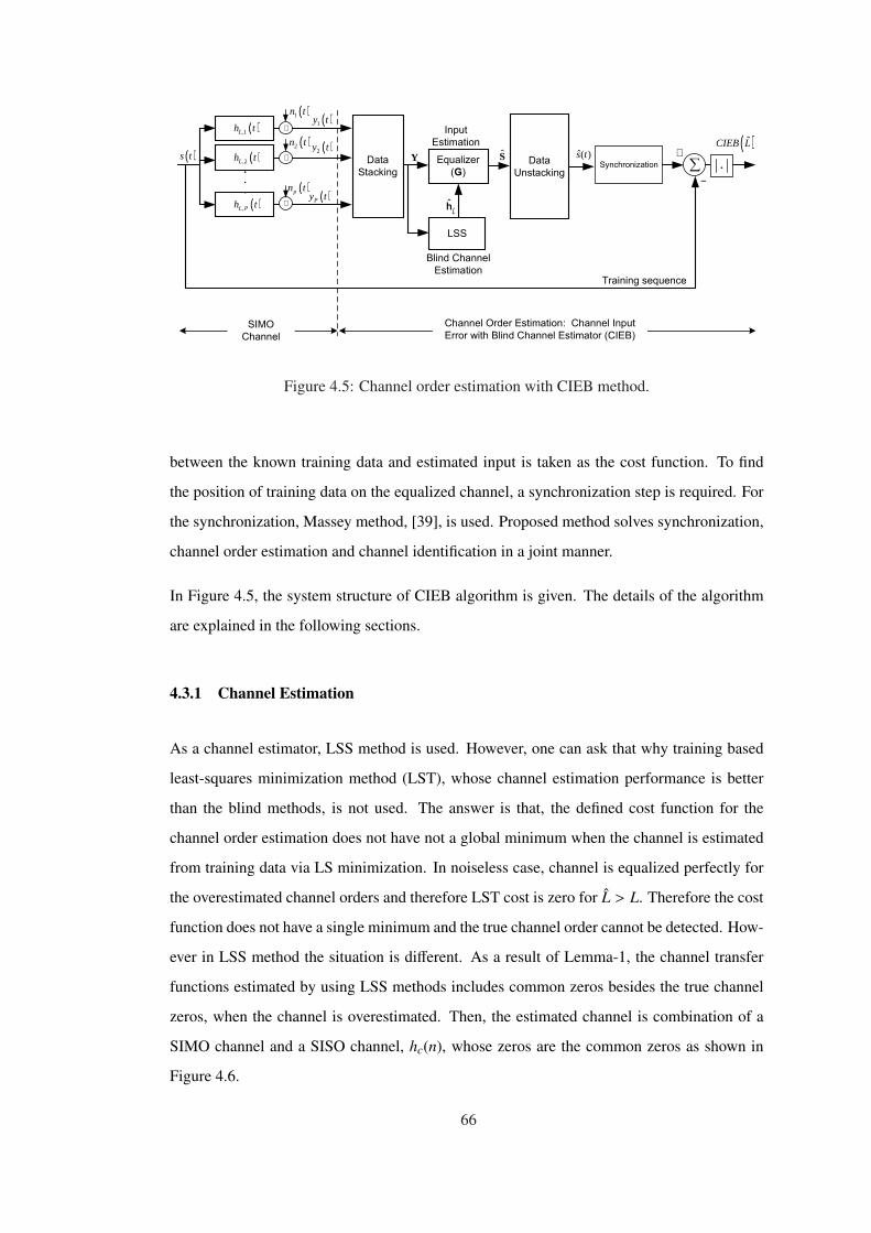
( )1y t

( )2y t

( )Py t

( )s t

( ),1Lh t

( ),2Lh t

( ),L Ph t

SYData

StackingData

Unstacking

Blind Channel

Estimation

Equalizer

(G)

LSS

Input

Estimation

SIMO

Channel

Channel Order Estimation: Channel Input

Error with Blind Channel Estimator (CIEB)

+∑

−

+

+

+

( )1n t

( )2n t

( )pn t

Synchronization

Training sequence

S ˆ( )s t( )ˆCIEB L

.

ˆˆL

h

Figure 4.5: Channel order estimation with CIEB method.

between the known training data and estimated input is taken as the cost function. To find

the position of training data on the equalized channel, a synchronization step is required. For

the synchronization, Massey method, [39], is used. Proposed method solves synchronization,

channel order estimation and channel identification in a joint manner.

In Figure 4.5, the system structure of CIEB algorithm is given. The details of the algorithm

are explained in the following sections.

4.3.1 Channel Estimation

As a channel estimator, LSS method is used. However, one can ask that why training based

least-squares minimization method (LST), whose channel estimation performance is better

than the blind methods, is not used. The answer is that, the defined cost function for the

channel order estimation does not have not a global minimum when the channel is estimated

from training data via LS minimization. In noiseless case, channel is equalized perfectly for

the overestimated channel orders and therefore LST cost is zero for L > L. Therefore the cost

function does not have a single minimum and the true channel order cannot be detected. How-

ever in LSS method the situation is different. As a result of Lemma-1, the channel transfer

functions estimated by using LSS methods includes common zeros besides the true channel

zeros, when the channel is overestimated. Then, the estimated channel is combination of a

SIMO channel and a SISO channel, hc(n), whose zeros are the common zeros as shown in

Figure 4.6.

66

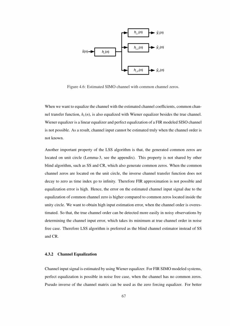
( )c

h n

,1( )

Lh n

,2( )

Lh n

, ( )L P

h n

( )s n

1( )y n

2ˆ ( )y n

ˆ ( )P

y n

Figure 4.6: Estimated SIMO channel with common channel zeros.

When we want to equalize the channel with the estimated channel coefficients, common chan-

nel transfer function, hc(n), is also equalized with Wiener equalizer besides the true channel.

Wiener equalizer is a linear equalizer and perfect equalization of a FIR modeled SISO channel

is not possible. As a result, channel input cannot be estimated truly when the channel order is

not known.

Another important property of the LSS algorithm is that, the generated common zeros are

located on unit circle (Lemma-3, see the appendix). This property is not shared by other

blind algorithm, such as SS and CR, which also generate common zeros. When the common

channel zeros are located on the unit circle, the inverse channel transfer function does not

decay to zero as time index go to infinity. Therefore FIR approximation is not possible and

equalization error is high. Hence, the error on the estimated channel input signal due to the

equalization of common channel zero is higher compared to common zeros located inside the

unity circle. We want to obtain high input estimation error, when the channel order is overes-

timated. So that, the true channel order can be detected more easily in noisy observations by

determining the channel input error, which takes its minimum at true channel order in noise

free case. Therefore LSS algorithm is preferred as the blind channel estimator instead of SS

and CR.

4.3.2 Channel Equalization

Channel input signal is estimated by using Wiener equalizer. For FIR SIMO modeled systems,

perfect equalization is possible in noise free case, when the channel has no common zeros.

Pseudo inverse of the channel matrix can be used as the zero forcing equalizer. For better

67

performance in noisy observations, MSE optimum Wiener equalizer is used. Wiener equalizer

is given as follows.

S = σ2sHH

M

(HMHH

M + σ2vI

)−1Y (4.13)

Wiener expression in (4.13) requires the knowledge of the signal and noise powers. For this

purpose, the method proposed in [36] is used.

4.3.3 Data Unstacking

By using Wiener equalization matrix, G, channel input matrix SM(t) is estimated. Channel

input sequence, s(t) is extracted from SM(t) by means of data unstacking operation. In data

unstacking operation, last L rows of the channel output matrix is deleted and resulted matrix

is vectorized.

4.3.4 Synchronization

Synchronization method varies depending on the frame transmission strategies (i.e periodic,

aperiodic, burst frame strategies), channel model (i.e., additive noise channel, flat fading chan-

nel and frequency selective channel) and where the synchronizer is applied at the receiver (i.e.,

before or after the equalizer). The most interesting work about frame synchronization was

done Massey, [39], for a continuous stream of BPSK data with a periodically inserted known

frame synchronization pattern. He developed the maximum likelihood (ML) frame synchro-

nization rule. The result is that classical correlators are not optimum way of synchronization

in AWGN in contrast common belief. ML rule consisted of a standard correlator followed

by a non-linear correction term accounting for the presence of random data surrounding the

known synchronization pattern. In the same work, the high- and low-SNR approximations

were also proposed to generated ML rules for practical systems. The ML criteria for Massey

is given as follows.

µ = maxµ

∣∣∣∣∣∣∣

T∑

t=1

ρt s(t + µ)

∣∣∣∣∣∣∣ −T∑

t=1

|s(t + µ)| (4.14)

where ρt, t = 1 . . .T , are the samples of the synchronization word. s is the received data

samples , and µ is the frame offset.

68

4.3.5 CIEB Cost Function

After estimating the input sequence and frame offset, the difference between the estimated

training data and training data is used as the cost function to determine the channel order.

Channel order that minimizes the cost function given below is taken as the channel order.

L = arg minL

N∑

k=1

T∑

t=1

∣∣∣sL (t + µ + kN) − s (t + µ)∣∣∣2 (4.15)

where sL indicates the estimated channel input sequence for the channel order, L. T is the

length of training sequence, N is the frame length and K is the number frames. The cost

function has a global minimum at the true channel order. When the channel order is underes-

timated, channel cannot be estimated by the LSS algorithm, hence the estimated channel input

signal is erroneous and cost function has a value greater than zero. When the channel order

is overestimated, common zeros are generated by the LSS algorithm in addition to the true

channel zeros. As mentioned before, this leads to errors on the estimated channel input sig-

nal. Therefore the cost function is greater than zero when the channel order is overestimated.

When the channel order is estimated correctly, channel coefficients are exactly estimated by

the LSS algorithm and channel input is estimated approximately. As a result, the cost function

has a global minimum at true channel order in noise free case.

4.4 Channel Order Estimation Using Semi-blind Channel Estimator and Train-

ing Data, (CIES)

A new method, CIES, is proposed for channel order estimation. CIES is the modified version

of CIEB to obtain a better performance in channel order estimation. The performance im-

provement is achieved by using a semi-blind channel estimation method instead of blind one.

For this purpose, semi-blind channel estimation method proposed in [38] is modified by using

LSS algorithm instead of SS method. Since a semi-blind method is used for channel estima-

tion, synchronization cannot be achieved as in CIEB. Here the synchronization is done after

the channel equalization. Synchronization problem in CIES is solved by jointly minimizing

the channel input error against channel order and frame offset. We show that the channel input

error is minimum when the channel order and frame offset is truly estimated.

The system structure of CIES method is given in Figure 4.7. The steps of the algorithms are

69

.

.

.

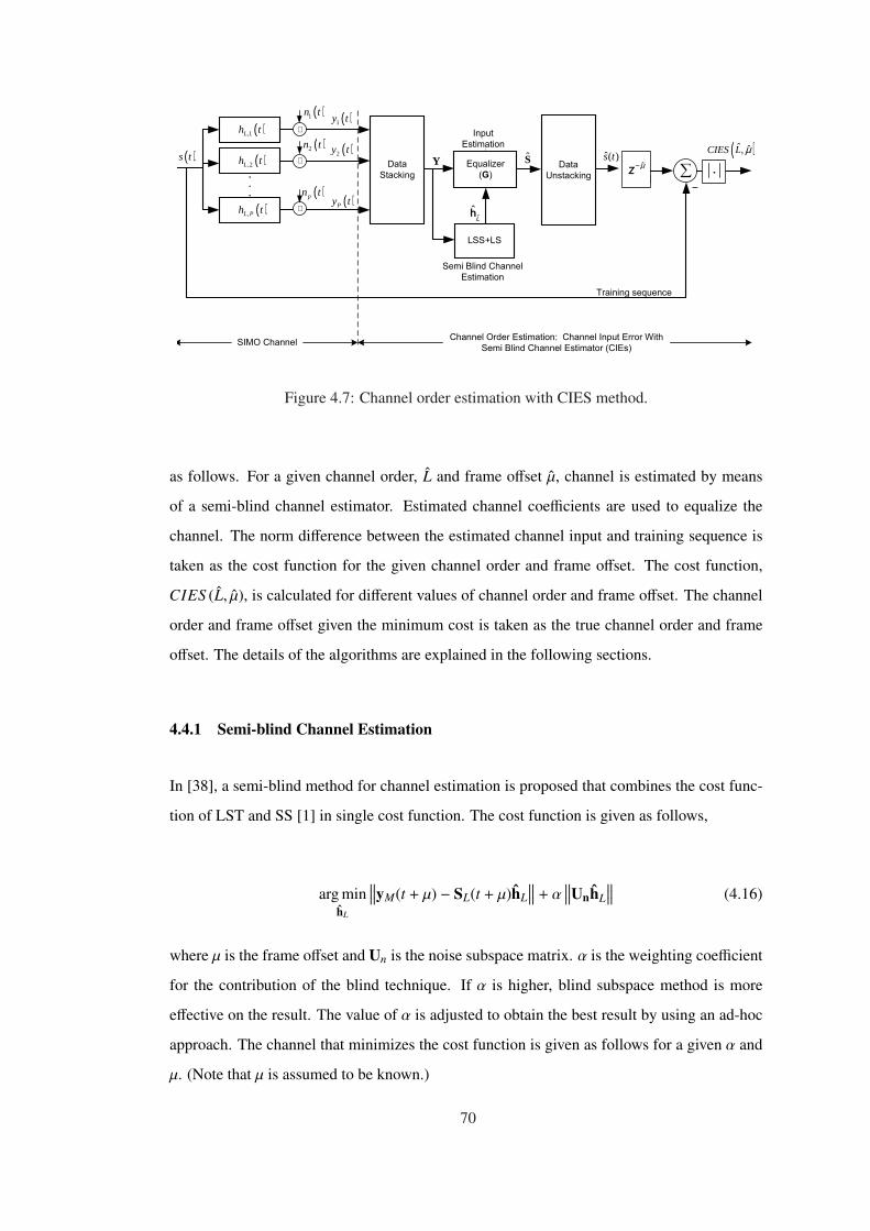
( )1y t

( )2y t

( )Py t

( )s t

( ),1Lh t

( ),2Lh t

( ),L Ph t

SYData

StackingData

Unstacking

Semi Blind Channel

Estimation

Equalizer

(G)

LSS+LS

Input

Estimation

SIMO ChannelChannel Order Estimation: Channel Input Error With

Semi Blind Channel Estimator (CIEs)

+∑

−

+

+

+

( )1n t

( )2n t

( )pn t

Training sequence

S ˆ( )s t ( )ˆ ˆ,µCIES L

ˆz

µ−.

ˆˆL

h

Figure 4.7: Channel order estimation with CIES method.

as follows. For a given channel order, L and frame offset µ, channel is estimated by means

of a semi-blind channel estimator. Estimated channel coefficients are used to equalize the

channel. The norm difference between the estimated channel input and training sequence is

taken as the cost function for the given channel order and frame offset. The cost function,

CIES (L, µ), is calculated for different values of channel order and frame offset. The channel

order and frame offset given the minimum cost is taken as the true channel order and frame

offset. The details of the algorithms are explained in the following sections.

4.4.1 Semi-blind Channel Estimation

In [38], a semi-blind method for channel estimation is proposed that combines the cost func-

tion of LST and SS [1] in single cost function. The cost function is given as follows,

arg minhL

∥∥∥yM(t + µ) − SL(t + µ)hL∥∥∥ + α

∥∥∥UnhL

∥∥∥ (4.16)

where µ is the frame offset and Un is the noise subspace matrix. α is the weighting coefficient

for the contribution of the blind technique. If α is higher, blind subspace method is more

effective on the result. The value of α is adjusted to obtain the best result by using an ad-hoc

approach. The channel that minimizes the cost function is given as follows for a given α and

µ. (Note that µ is assumed to be known.)

70

hL =(SH

L (t + µ)SL(t + µ) + αUHn Un

)†SH

L (t + µ)yM(t + µ) (4.17)

Semi-blind channel estimation algorithm proposed in [38] is modified by using LSS algorithm

instead of the SS method. In this way, a better algorithm is obtained in terms of estimating the

channel order in noisy observations. This is due to the fact that when the channel is estimated

by LSS with overestimated channel order, common zeros produced by the LSS algorithm

are placed on the unit circle. This leads to high error in the equalization step of CIES and

generates deeper valleys at the true channel order at the cost function defined for CIES.

LSS algorithm minimizes the cost function below to find the channel coefficients up to a scale

factor, i.e.,

arg minhL

∥∥∥QhL

∥∥∥ (4.18)

where Q is constructed from the null space of the smoothing error matrix, E, in LSS method.

(For the detail refer to the Chapter 2.) LST minimizes the following the cost function using

only the received signal which contains the training sequence, i.e.,

arg minhL

∥∥∥yM(t + µ) − SL(t + µ)hL∥∥∥ (4.19)

where SL(t + µ) is constructed from the training sequence. The combined cost function is

defined as follows,

arg minhL

∥∥∥yM(t + µ) − SL(t + µ)hL∥∥∥ + α

∥∥∥QhL

∥∥∥ (4.20)

with the solution given as follows,

hL =(SH

L (t + µ)SL(t + µ) + αQHQ)†

SHL (t + µ)yM(t + µ) (4.21)

The value of α determines the effect of LSS on the channel estimation. It should be adjusted to

obtain the best result. When α = 0, it is a training based LS method and channel order cannot

be found properly in noisy observations. When α = ∞, it becomes to the CIEB method. By

adjusting α, the channel estimation performance can be increased beyond LSS.

71

4.4.2 CIES Cost Function

CIES uses the channel input error, s(t) − s(t), for the estimation of channel order and frame

offset and given as follows.

CIES (L, µ) =

K∑

k=1

T∑

t=1

∣∣∣s(L)(t + µ + kN) − s(t + µ)∣∣∣2 (4.22)

L, µ = arg minL,µ

CIES (L, µ) (4.23)

(4.24)

where T is the length of the training sequence, N is the frame length and K is the number

frames. The defined cost function, CIES, has global minimum at the true channel order and

frame offset. Semi-blind method used in CIES is a deterministic method and channel coeffi-

cient can be found exactly from finite number of samples in noise free case when the channel

order and frame offset is known. Therefore, CIES cost function is zero when the channel

order and frame offset is correctly estimated. When the synchronization is not achieved, LST

does not work and channel cannot be estimated. Therefore synchronization is a pre-request.

When the channel order is underestimated, LSS and LST cannot estimate the channel coeffi-

cients. When the channel order is overestimated, LSS finds the channel transfer function with

additional common channel zeros. This leads equalization error in estimated channel input.

Therefore, the cost function will be greater than zero when the channel order is overestimated.

As a result, the cost function is zero only if the channel order and frame offset is correctly

estimated.

4.4.3 Simulations

Several experiments for different channel orders and number of sub-channels were realized for

the performance comparison. The common simulation settings are as follows. , the number of

frames is K = 2 and frame length is 100. As a training sequence (which is also synchroniza-

tion word) 13 bit Barker code is used. As a modulation waveform, BPSK is used. For a fair

comparison, after the channel order is estimated by the algorithms, channel is estimated with

LSS and equalized with Wiener equalizer for all blind channel order estimation algorithms.

In CIES algorithm, the value of α is set to α = 100. Frame offset is µ = 3. Frame offset is

72

searched in the set µ = 1 . . . 5 for frame synchronization. Channel order is searched in the set

L = 1 . . . L + 6 in all algorithms. 1000 trials are evaluated at each SNR level to compute the

probability of correct channel order estimation and BER. SNR is computed as follows,

S NR =1

Pσ2 E

P∑

j=1

∣∣∣y j (k)∣∣∣2 (4.25)

where P is the number of channel outputs, σ2 is the noise variance and y j (k) is the noiseless

samples of the jth output.

In Figure 4.8, probability of correct channel order estimation and BER is plotted against SNR

for L = 3 and P = 3. As seen from the Figure 4.8, proposed methods are better than the blind

methods except CMR and COE in a wide SNR range. Performance of CIES is close to COE

and worse than CMR in channel order estimation. On the other hand, COES has lower BER

than COE when S NR > 12dB. Although CIEB performs worse than CIES, CMR and COE

in channel order estimation, resulted BER in CMR, CIEB and CIES are nearly same.

The same experiment is done for L = 5, P = 3; and L = 5, P = 5 in Figure 4.9 and Figure

4.10 respectively. Channel order estimation performance of CIES increases when the number

of channel increases and became similar with the CMR, which is the best one. Performance

increment is also affected the BER of CIES and lowest BER is obtained by this method, when

S NR > 12dB. Channel order estimation of CIEB also increases with the number of channel;

however this increment is no enough to make it better than COE and CMR. On the other hand,

BER performance is nearly same with CMR and better than COE when the channel order is

also increased.

73

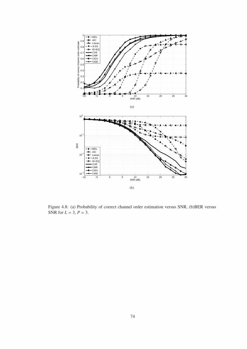
−10 −5 0 5 10 15 20 25 300

0.1

0.2

0.3

0.4

0.5

0.6

0.7

0.8

0.9

1

SNR (dB)

Pro

babi

lity

of c

orre

ct c

hann

el o

rder

est

imat

e

MDLAICLiavasJLSSID+EQCOECMRCIESCIEB

(a)

−10 −5 0 5 10 15 20 25 3010

−3

10−2

10−1

100

SNR (dB)

BE

R


(b)

Figure 4.8: (a) Probability of correct channel order estimation versus SNR, (b)BER versusSNR for L = 3, P = 3.

74

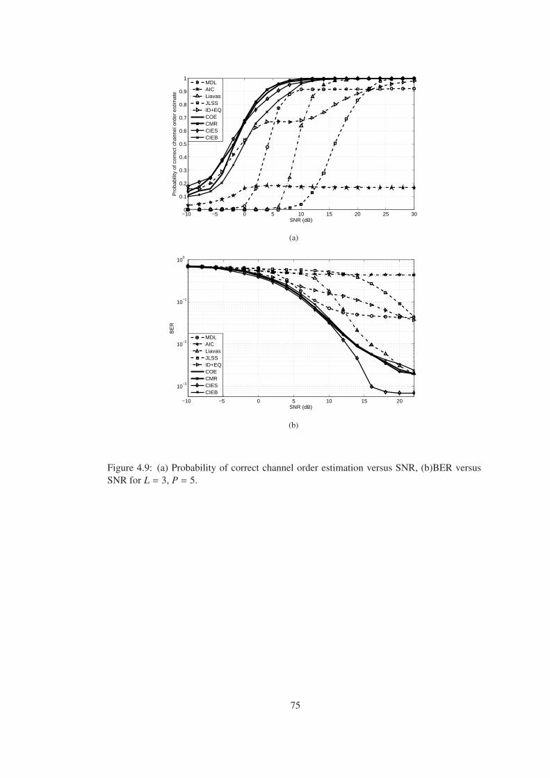
−10 −5 0 5 10 15 20 25 300

0.1

0.2

0.3

0.4

0.5

0.6

0.7

0.8

0.9

1

SNR (dB)

Pro

babi

lity

of c

orre

ct c

hann

el o

rder

est

imat

e


(a)

−10 −5 0 5 10 15 20

10−3

10−2

10−1

100

SNR (dB)

BE

R


(b)


75

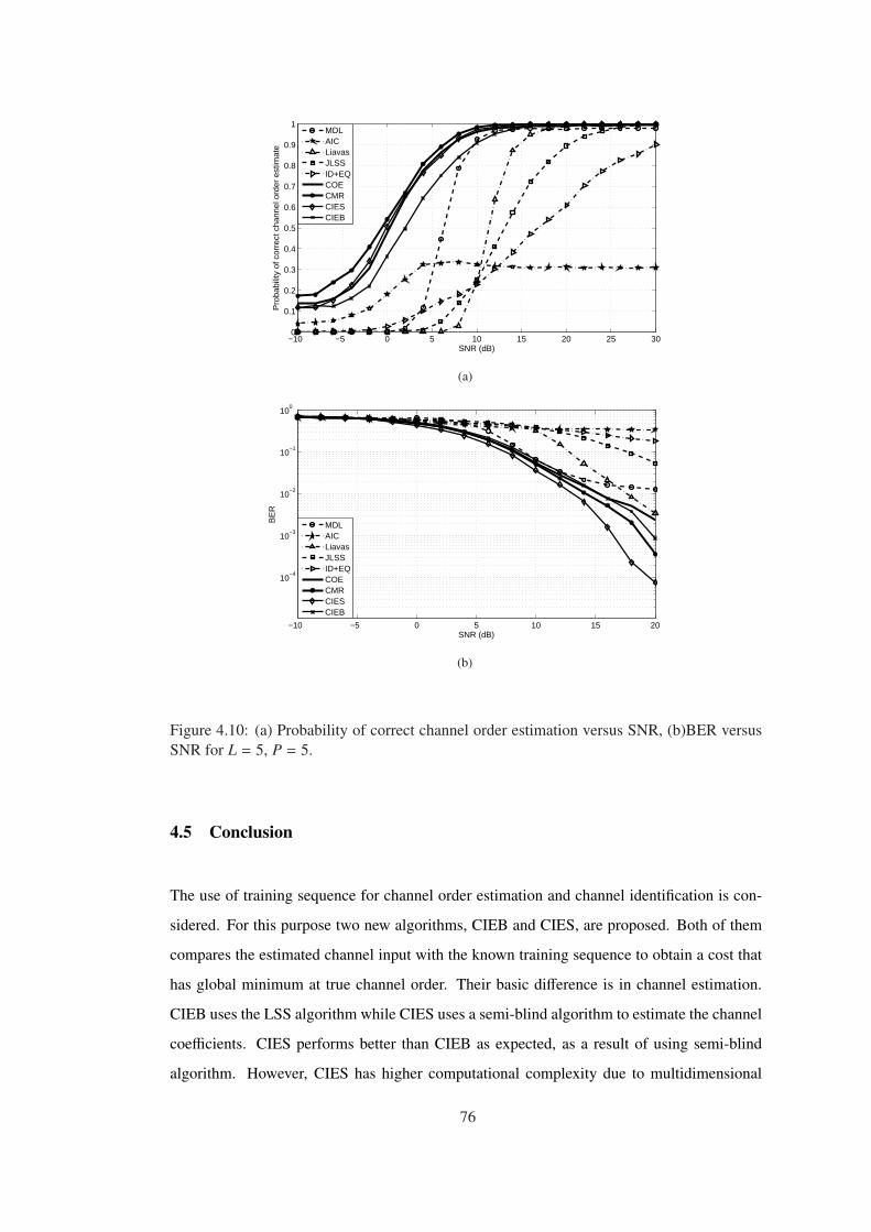
−10 −5 0 5 10 15 20 25 300

0.1

0.2

0.3

0.4

0.5

0.6

0.7

0.8

0.9

1

SNR (dB)

Pro

babi

lity

of c

orre

ct c

hann

el o

rder

est

imat

e


(a)

−10 −5 0 5 10 15 20

10−4

10−3

10−2

10−1

100

SNR (dB)

BE

R


(b)


4.5 Conclusion

The use of training sequence for channel order estimation and channel identification is con-

sidered. For this purpose two new algorithms, CIEB and CIES, are proposed. Both of them

compares the estimated channel input with the known training sequence to obtain a cost that

has global minimum at true channel order. Their basic difference is in channel estimation.

CIEB uses the LSS algorithm while CIES uses a semi-blind algorithm to estimate the channel

coefficients. CIES performs better than CIEB as expected, as a result of using semi-blind

algorithm. However, CIES has higher computational complexity due to multidimensional

76

search done for joint frame synchronization and channel order estimation. When the training

based methods are compared with the blind methods COE and CMR, there is no significant

improvement for the channel order estimation. However, resulted BER in CIES is lower

when S NR > 12dB and improvement in BER becomes more significant when the number of

channel is increased.

77

CHAPTER 5

EFFECTIVE CHANNEL ORDER ESTIMATION

5.1 Introduction

Effective channel order estimation is the task of finding the significant part of the channel

filter. Figure 5.1 shows a generic channel filter impulse response. In this figure, the impulse

response has large and small coefficients. Large coefficients can be assumed to be surrounded

by the small coefficients which are called as leading and trailing tails without loss of gener-

ality. The distinction between tails and the significant part of the channel coefficients can be

made by considering a threshold amplitude γ/2. The coefficients whose magnitudes are above

γ/2 may be defined as the significant part of the filter. Obviously the value of γ/2 for deter-

mining the significant part depends on certain factors including SNR and the cost function or

the measure used to define the significant part. When the SNR is very large, the true channel

order can be defined to be the whole filter including the tail coefficients. When the SNR is

low, it may not be possible to clearly identify the tail coefficients. It may also be meaningless

to try to find those coefficients since the channel equalization performed over the noisy output

samples does not give better MSE for the input samples when the tail coefficients are used

due to noise amplification for the small channel coefficients. Therefore in practice, the task

is to find the effective channel order which corresponds to finding the significant part of the

channel filter rather than the true channel order. In fact in blind problem, it may be impossible

to find the true channel order from the noisy output samples. True channel order has meaning

when the SNR is very large or when the channel order estimation algorithms are tested by as-

suming that the channel filter is known. In this thesis, different channel filters, including fixed

and random long channels with tails and channels without the tails are considered. Note that

when there are no tails, true channel order and effective channel order become same. It should

78

also be pointed that when we consider the channels without tails, the channel coefficients are

generated randomly to obtain a Rayleigh distribution.

In practice, finding the effective channel order is more important than finding the true channel

order, especially for the cases when the channel has leading and trailing tail coefficients. This

is mainly due to the fact that channel matrix becomes ill-conditioned, when the channel in-

cludes small tail coefficients. In [22], the effect of small leading and trailing tails for subspace

(SS) channel identification/equalization methods are investigated. It is shown that when the

channel order is overestimated (i.e., the estimated channel includes a part of tail/head coef-

ficients besides the significant part of the channel), the performance of LS and SS methods

in channel estimation degrades dramatically. Therefore estimating the effective channel order

is important for the improvement of the performance of blind channel estimation algorithms

and obtaining better BER.

In [5], a channel order estimation algorithm is proposed for the effective channel order es-

timation. This algorithm is based on numerical analysis arguments and essentially consider

the gap between the two consecutive eigenvalues of the estimated covariance matrix. In [4],

information theoretic algorithms are analyzed and compared with [5] where the algorithm is

shown to work well at high SNR. In [47], a criteria is presented to determine the effective

channel order when the channel filter is known. In this thesis, this criteria is used to deter-

mine the effective channel order for a given channel filter. In addition, bit-error-rate (BER) is

used as a measure to test the performance of the order estimation algorithms. The proposed

methods for channel order estimation are analyzed under effective channel order concept. It

is shown that COE and CMR are significantly better than other blind methods especially at

low SNR and they tend to estimate the effective channel order when the search set does not

include the true channel order. When the search set includes the true channel order, they tend

to find true channel order at high SNR. The SNR range, where the effective channel order is

mostly estimated, is larger than the alternative algorithms and better BER is obtained.

Channel order is an important parameter for channel estimation and equalization. Best perfor-

mance is achieved when the effective channel order is correctly estimated. However, due to

non existence of high performance of channel order estimation algorithms, this problem has

been solved with the channel estimation algorithms robust to channel order overestimation

or with non-linear adaptive equalizer such as DFE. It is known that their performance is not

79

good as the their deterministic alternatives such as SS, CR and LSS which has superior per-

formance when the channel order is known. On the another hand, the main drawback of blind

deterministic algorithms is that their performances decreases dramatically when the channel

order is not correctly estimated. Therefore the use of these algorithms is not practical as a

consequence of absence of high performance channel order estimation algorithms. In this

thesis, it is shown that when the proposed algorithms COE and CMR are used, determinis-

tic blind algorithms can be used effectively and significant performance improvement can be

achieved compared to LP based algorithms and fractionally spaced DFE which not require

exact knowledge of the channel order.

Proposed semi-blind algorithms, CIES and CIEB are also evaluated and compared with the

blind algorithms to see the gain of using training symbols in effective channel order estima-

tion. In chapter 4, it is seen that the training based techniques do not offer much when the

true channel order is considered. This is not the case, when the effective channel order es-

timation is considered. It is shown that CIES performs better than blind algorithms due to

better channel estimation with pilots, when the final BER is considered. However, the main

drawback of this algorithm is the high computational cost due to the multidimentional search

for synchronization.

80

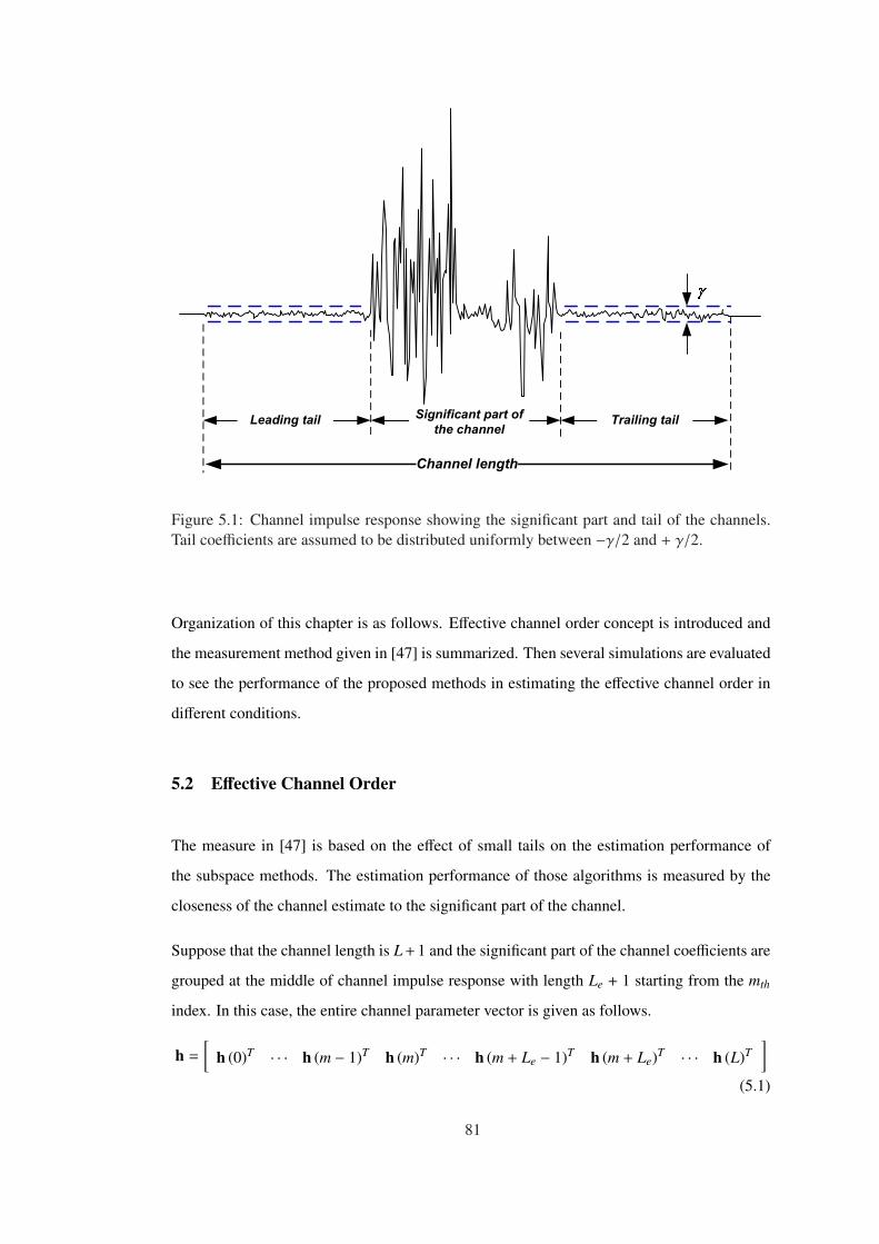
Significant part of

the channelLeading tail Trailing tail

Channel length

Figure 5.1: Channel impulse response showing the significant part and tail of the channels.Tail coefficients are assumed to be distributed uniformly between −γ/2 and + γ/2.

Organization of this chapter is as follows. Effective channel order concept is introduced and

the measurement method given in [47] is summarized. Then several simulations are evaluated

to see the performance of the proposed methods in estimating the effective channel order in

different conditions.

5.2 Effective Channel Order

The measure in [47] is based on the effect of small tails on the estimation performance of

the subspace methods. The estimation performance of those algorithms is measured by the

closeness of the channel estimate to the significant part of the channel.

Suppose that the channel length is L + 1 and the significant part of the channel coefficients are

grouped at the middle of channel impulse response with length Le + 1 starting from the mth

index. In this case, the entire channel parameter vector is given as follows.

h =

[h (0)T · · · h (m − 1)T h (m)T · · · h (m + Le − 1)T h (m + Le)T · · · h (L)T

]

(5.1)

81

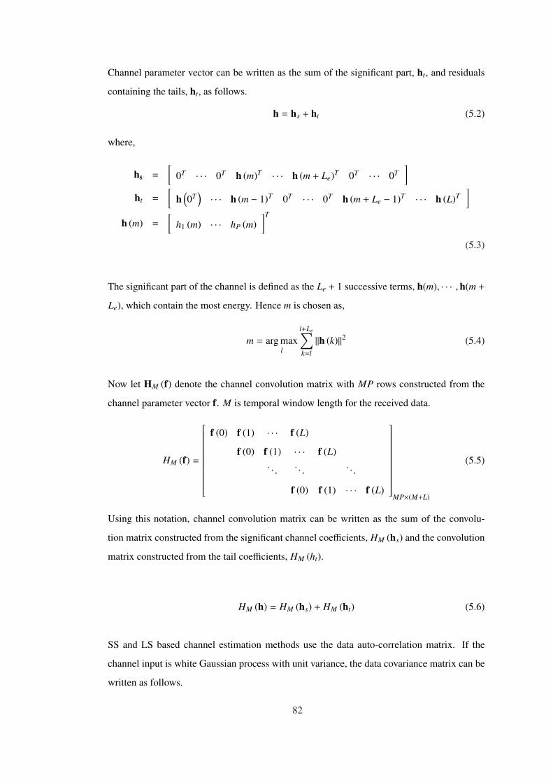
Channel parameter vector can be written as the sum of the significant part, ht, and residuals

containing the tails, ht, as follows.

h = hs + ht (5.2)

where,

hs =

[0T · · · 0T h (m)T · · · h (m + Le)T 0T · · · 0T

]

ht =

[h(0T

)· · · h (m − 1)T 0T · · · 0T h (m + Le − 1)T · · · h (L)T

]

h (m) =

[h1 (m) · · · hP (m)

]T

(5.3)

The significant part of the channel is defined as the Le + 1 successive terms, h(m), · · · ,h(m +

Le), which contain the most energy. Hence m is chosen as,

m = arg maxl

l+Le∑

k=l

‖h (k)‖2 (5.4)

Now let HM (f) denote the channel convolution matrix with MP rows constructed from the

channel parameter vector f. M is temporal window length for the received data.

HM (f) =

f (0) f (1) · · · f (L)

f (0) f (1) · · · f (L). . .

. . .. . .

f (0) f (1) · · · f (L)

MP×(M+L)

(5.5)

Using this notation, channel convolution matrix can be written as the sum of the convolu-

tion matrix constructed from the significant channel coefficients, HM (hs) and the convolution

matrix constructed from the tail coefficients, HM (ht).

HM (h) = HM (hs) + HM (ht) (5.6)

SS and LS based channel estimation methods use the data auto-correlation matrix. If the

channel input is white Gaussian process with unit variance, the data covariance matrix can be

written as follows.

82

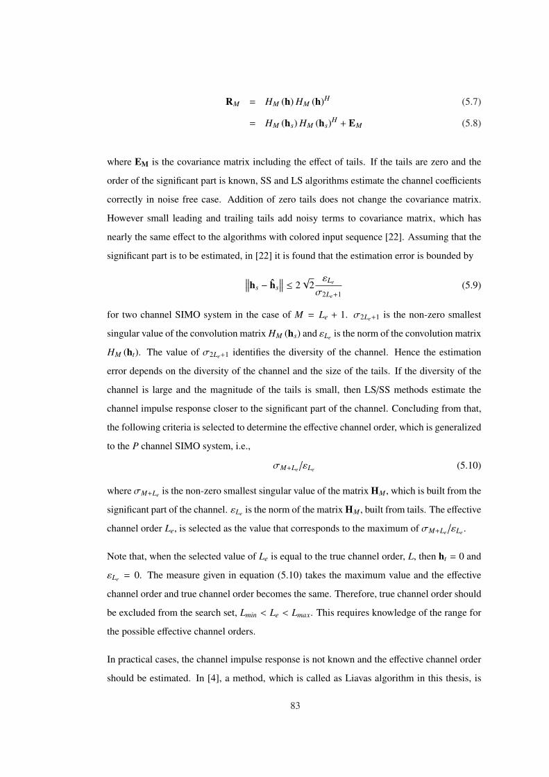
RM = HM (h) HM (h)H (5.7)

= HM (hs) HM (hs)H + EM (5.8)

where EM is the covariance matrix including the effect of tails. If the tails are zero and the

order of the significant part is known, SS and LS algorithms estimate the channel coefficients

correctly in noise free case. Addition of zero tails does not change the covariance matrix.

However small leading and trailing tails add noisy terms to covariance matrix, which has

nearly the same effect to the algorithms with colored input sequence [22]. Assuming that the

significant part is to be estimated, in [22] it is found that the estimation error is bounded by

∥∥∥hs − hs∥∥∥ ≤ 2

√2

εLe

σ2Le+1(5.9)

for two channel SIMO system in the case of M = Le + 1. σ2Le+1 is the non-zero smallest

singular value of the convolution matrix HM (hs) and εLe is the norm of the convolution matrix

HM (ht). The value of σ2Le+1 identifies the diversity of the channel. Hence the estimation

error depends on the diversity of the channel and the size of the tails. If the diversity of the

channel is large and the magnitude of the tails is small, then LS/SS methods estimate the

channel impulse response closer to the significant part of the channel. Concluding from that,

the following criteria is selected to determine the effective channel order, which is generalized

to the P channel SIMO system, i.e.,

σM+Le

/εLe (5.10)

where σM+Le is the non-zero smallest singular value of the matrix HM, which is built from the

significant part of the channel. εLe is the norm of the matrix HM, built from tails. The effective

channel order Le, is selected as the value that corresponds to the maximum of σM+Le

/εLe .

Note that, when the selected value of Le is equal to the true channel order, L, then ht = 0 and

εLe = 0. The measure given in equation (5.10) takes the maximum value and the effective

channel order and true channel order becomes the same. Therefore, true channel order should

be excluded from the search set, Lmin < Le < Lmax. This requires knowledge of the range for

the possible effective channel orders.

In practical cases, the channel impulse response is not known and the effective channel order

should be estimated. In [4], a method, which is called as Liavas algorithm in this thesis, is

83

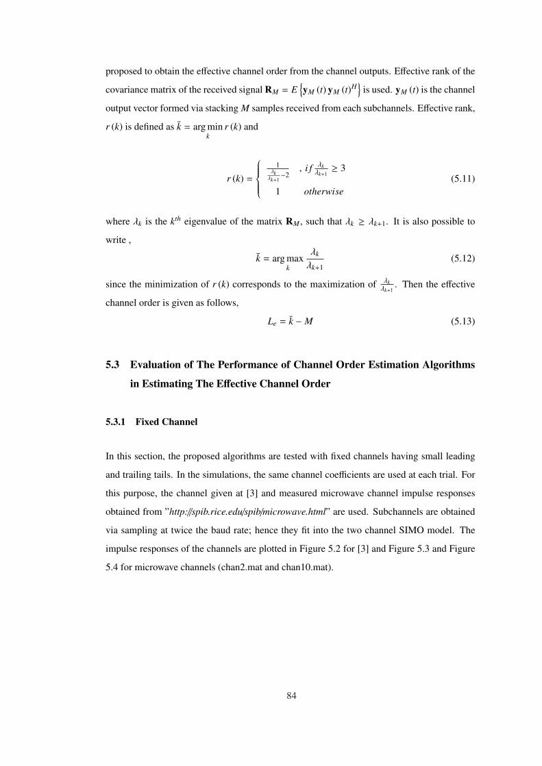
proposed to obtain the effective channel order from the channel outputs. Effective rank of the

covariance matrix of the received signal RM = E{yM (t) yM (t)H

}is used. yM (t) is the channel

output vector formed via stacking M samples received from each subchannels. Effective rank,

r (k) is defined as k = arg mink

r (k) and

r (k) =

1λkλk+1−2

, i f λkλk+1≥ 3

1 otherwise(5.11)

where λk is the kth eigenvalue of the matrix RM , such that λk ≥ λk+1. It is also possible to

write ,

k = arg maxk

λk

λk+1(5.12)

since the minimization of r (k) corresponds to the maximization of λkλk+1

. Then the effective

channel order is given as follows,

Le = k − M (5.13)

5.3 Evaluation of The Performance of Channel Order Estimation Algorithms

in Estimating The Effective Channel Order

5.3.1 Fixed Channel

In this section, the proposed algorithms are tested with fixed channels having small leading

and trailing tails. In the simulations, the same channel coefficients are used at each trial. For

this purpose, the channel given at [3] and measured microwave channel impulse responses

obtained from ”http://spib.rice.edu/spib/microwave.html” are used. Subchannels are obtained

via sampling at twice the baud rate; hence they fit into the two channel SIMO model. The

impulse responses of the channels are plotted in Figure 5.2 for [3] and Figure 5.3 and Figure

5.4 for microwave channels (chan2.mat and chan10.mat).

84

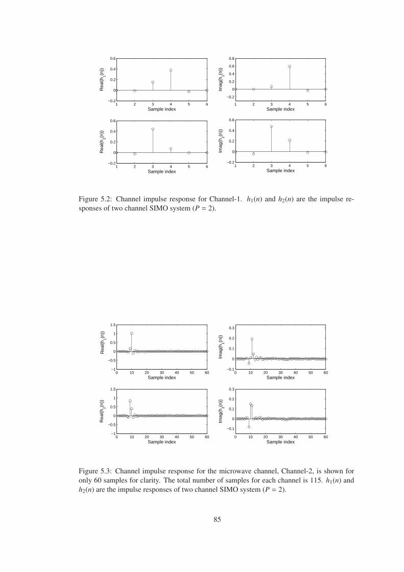
1 2 3 4 5 6−0.2

0

0.2

0.4

0.6

Sample index

Rea

l(h1(n

))1 2 3 4 5 6

−0.2

0

0.2

0.4

0.6

0.8

Sample index

Imag

(h1(n

))

1 2 3 4 5 6−0.2

0

0.2

0.4

0.6

Sample index

Rea

l(h2(n

))

1 2 3 4 5 6−0.2

0

0.2

0.4

0.6

Sample index

Imag

(h2(n

))

Figure 5.2: Channel impulse response for Channel-1. h1(n) and h2(n) are the impulse re-sponses of two channel SIMO system (P = 2).

0 10 20 30 40 50 60−1

−0.5

0

0.5

1

1.5

Sample index

Rea

l(h1(n

))

0 10 20 30 40 50 60−0.1

0

0.1

0.2

0.3

Sample index

Imag

(h1(n

))

0 10 20 30 40 50 60−1

−0.5

0

0.5

1

1.5

Sample index

Rea

l(h2(n

))

0 10 20 30 40 50 60

−0.1

0

0.1

0.2

0.3

Sample index

Imag

(h2(n

))

Figure 5.3: Channel impulse response for the microwave channel, Channel-2, is shown foronly 60 samples for clarity. The total number of samples for each channel is 115. h1(n) andh2(n) are the impulse responses of two channel SIMO system (P = 2).

85

0 10 20 30 40 50 60−0.5

0

0.5

1

Sample indexR

eal(h

1(n))

0 10 20 30 40 50 60−0.1

0

0.1

0.2

0.3

Sample index

Imag

(h1(n

))

0 10 20 30 40 50 60−0.5

0

0.5

1

Sample index

Rea

l(h2(n

))

0 10 20 30 40 50 60−0.2

−0.1

0

0.1

0.2

Sample index

Imag

(h2(n

))

Figure 5.4: Channel impulse response for the microwave channel, Channel-3, is shown foronly 60 samples for clarity. The total number of samples for each channel is 150. h1(n) andh2(n) are the impulse responses of two channel SIMO system (P = 2).

The effective channel order is determined using the criteria σ2Le+1εLe

for the selected channels. In

Figure 5.5, the value of the criteria given by equation 5.10 ( also called as condition measure)

is plotted against the channel order. The index which gives the maximum value is taken

as the effective channel order. As seen from the Figure 5.5, the effective channel order is

one for the Channel-1 and Channel-2, and two for Channel-3. Condition measure not only

gives information about the effective length of the significant part. But it also shows whether

the channel is ill-conditioned or not. When the condition measure is lower, the signal and

noise spaces are closer and it is hard to separate them in noisy measurements. Therefore

channel estimation error increases in subspace based methods. This is also related to the rank

of the channel matrix. The channel matrix should be of full column rank for blind channel

estimation algorithms. If the diversity is zero, which is the case when the condition measure

is zero, channel matrix is not of full column rank. Hence, proper channel estimation is not

possible. As a result, when the condition measure is low the estimation of effective channel

order and the channel coefficient is problematic. In this respect, Channel-3 can be said to be an

ill-conditioned channel compared to the others. The condition measure is defined originally

for the SS based methods, and finds the channel order which leads to maximumly separable

subspaces. Therefore, effective channel order measured through condition measure may be

different for other blind channel estimation algorithms, such as LSS. To clarify this point for

86

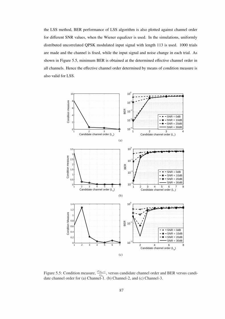
the LSS method, BER performance of LSS algorithm is also plotted against channel order

for different SNR values, when the Wiener equalizer is used. In the simulations, uniformly

distributed uncorrelated QPSK modulated input signal with length 113 is used. 1000 trials

are made and the channel is fixed, while the input signal and noise change in each trial. As

shown in Figure 5.5, minimum BER is obtained at the determined effective channel order in

all channels. Hence the effective channel order determined by means of condition measure is

also valid for LSS.

1 2 3 40

2

4

6

8

10

Candidate channel order (Le)

Con

ditio

n m

easu

re

1 2 3 410

−4

10−3

10−2

10−1

100


BE

R

SNR = 0dBSNR = 10dBSNR = 20dBSNR = 30dB

(a)

1 2 3 4 5 6 70

0.5

1

1.5

2

2.5

3

3.5


Con

ditio

n m

easu

re

1 2 3 4 5 6 7 810

−3

10−2

10−1

100


BE

R


(b)

1 2 3 4 5 6 70

0.2

0.4

0.6

0.8

1

1.2

1.4

Con

ditio

n M

easu

re

2 4 6 810

−2

10−1

100


BE

R


(c)

Figure 5.5: Condition measure, σ2Le+1εLe

, versus candidate channel order and BER versus candi-date channel order for (a) Channel-1. (b) Channel-2, and (c) Channel-3.

87

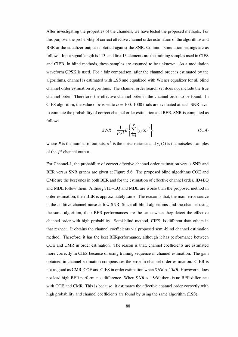
After investigating the properties of the channels, we have tested the proposed methods. For

this purpose, the probability of correct effective channel order estimation of the algorithms and

BER at the equalizer output is plotted against the SNR. Common simulation settings are as

follows. Input signal length is 113, and first 13 elements are the training samples used in CIES

and CIEB. In blind methods, these samples are assumed to be unknown. As a modulation

waveform QPSK is used. For a fair comparison, after the channel order is estimated by the

algorithms, channel is estimated with LSS and equalized with Wiener equalizer for all blind

channel order estimation algorithms. The channel order search set does not include the true

channel order. Therefore, the effective channel order is the channel order to be found. In

CIES algorithm, the value of α is set to α = 100. 1000 trials are evaluated at each SNR level

to compute the probability of correct channel order estimation and BER. SNR is computed as

follows.

S NR =1

Pσ2 E

P∑

j=1

∣∣∣y j (k)∣∣∣2 (5.14)

where P is the number of outputs, σ2 is the noise variance and y j (k) is the noiseless samples

of the jth channel output.

For Channel-1, the probability of correct effective channel order estimation versus SNR and

BER versus SNR graphs are given at Figure 5.6. The proposed blind algorithms COE and

CMR are the best ones in both BER and for the estimation of effective channel order. ID+EQ

and MDL follow them. Although ID+EQ and MDL are worse than the proposed method in

order estimation, their BER is approximately same. The reason is that, the main error source

is the additive channel noise at low SNR. Since all blind algorithms find the channel using

the same algorithm, their BER performances are the same when they detect the effective

channel order with high probability. Semi-blind method, CIES, is different than others in

that respect. It obtains the channel coefficients via proposed semi-blind channel estimation

method. Therefore, it has the best BERperformance, although it has performance between

COE and CMR in order estimation. The reason is that, channel coefficients are estimated

more correctly in CIES because of using training sequence in channel estimation. The gain

obtained in channel estimation compensates the error in channel order estimation. CIEB is

not as good as CMR, COE and CIES in order estimation when S NR < 15dB. However it does

not lead high BER performance difference. When S NR > 15dB, there is no BER difference

with COE and CMR. This is because, it estimates the effective channel order correctly with

high probability and channel coefficients are found by using the same algorithm (LSS).

88

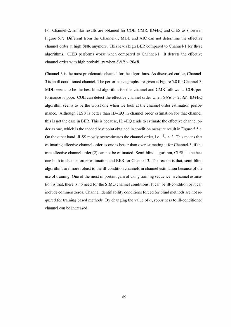
For Channel-2, similar results are obtained for COE, CMR, ID+EQ and CIES as shown in

Figure 5.7. Different from the Channel-1, MDL and AIC can not determine the effective

channel order at high SNR anymore. This leads high BER compared to Channel-1 for these

algorithms. CIEB performs worse when compared to Channel-1. It detects the effective

channel order with high probability when S NR > 20dB.

Channel-3 is the most problematic channel for the algorithms. As discussed earlier, Channel-

3 is an ill conditioned channel. The performance graphs are given at Figure 5.8 for Channel-3.

MDL seems to be the best blind algorithm for this channel and CMR follows it. COE per-

formance is poor. COE can detect the effective channel order when S NR > 25dB. ID+EQ

algorithm seems to be the worst one when we look at the channel order estimation perfor-

mance. Although JLSS is better than ID+EQ in channel order estimation for that channel,

this is not the case in BER. This is because, ID+EQ tends to estimate the effective channel or-

der as one, which is the second best point obtained in condition measure result in Figure 5.5.c.

On the other hand, JLSS mostly overestimates the channel order, i.e., Le > 2. This means that

estimating effective channel order as one is better than overestimating it for Channel-3, if the

true effective channel order (2) can not be estimated. Semi-blind algorithm, CIES, is the best

one both in channel order estimation and BER for Channel-3. The reason is that, semi-blind

algorithms are more robust to the ill-condition channels in channel estimation because of the

use of training. One of the most important gain of using training sequence in channel estima-

tion is that, there is no need for the SIMO channel conditions. It can be ill-condition or it can

include common zeros. Channel identifiability conditions forced for blind methods are not re-

quired for training based methods. By changing the value of α, robustness to ill-conditioned

channel can be increased.

89

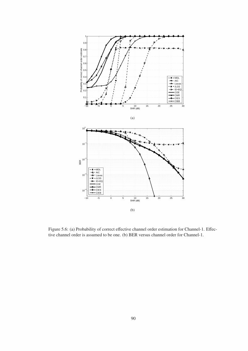
−10 −5 0 5 10 15 20 25 300

0.1

0.2

0.3

0.4

0.5

0.6

0.7

0.8

0.9

1

SNR (dB)

Pro

babi

lity

of c

orre

ct c

hann

el o

rder

est

imat

e


(a)

−10 −5 0 5 10 15 20 25 30

10−4

10−3

10−2

10−1

100

SNR (dB)

BE

R


(b)

Figure 5.6: (a) Probability of correct effective channel order estimation for Channel-1. Effec-tive channel order is assumed to be one. (b) BER versus channel order for Channel-1.

90

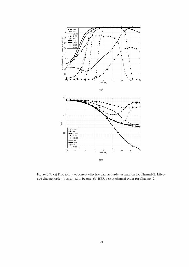
−10 −5 0 5 10 15 20 25 300

0.1

0.2

0.3

0.4

0.5

0.6

0.7

0.8

0.9

1

SNR (dB)

Pro

babi

lity

of c

orre

ct c

hann

el o

rder

est

imat

e


(a)

−10 −5 0 5 10 15 20 25 30

10−2

10−1

100

SNR (dB)

BE

R


(b)

Figure 5.7: (a) Probability of correct effective channel order estimation for Channel-2. Effec-tive channel order is assumed to be one. (b) BER versus channel order for Channel-2.

91

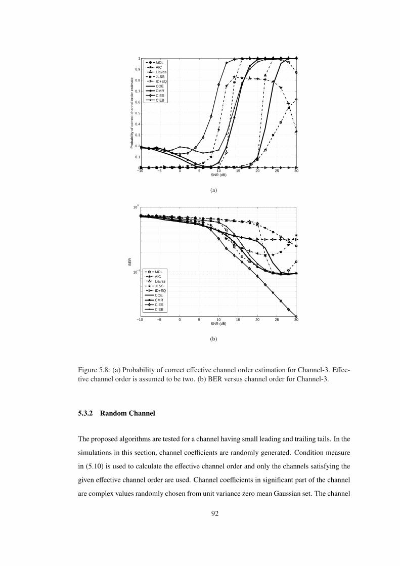
−10 −5 0 5 10 15 20 25 300

0.1

0.2

0.3

0.4

0.5

0.6

0.7

0.8

0.9

1

SNR (dB)

Pro

babi

lity

of c

orre

ct c

hann

el o

rder

est

imat

e


(a)

−10 −5 0 5 10 15 20 25 30

10−1

100

SNR (dB)

BE

R


(b)

Figure 5.8: (a) Probability of correct effective channel order estimation for Channel-3. Effec-tive channel order is assumed to be two. (b) BER versus channel order for Channel-3.

5.3.2 Random Channel

The proposed algorithms are tested for a channel having small leading and trailing tails. In the

simulations in this section, channel coefficients are randomly generated. Condition measure

in (5.10) is used to calculate the effective channel order and only the channels satisfying the

given effective channel order are used. Channel coefficients in significant part of the channel

are complex values randomly chosen from unit variance zero mean Gaussian set. The channel

92

coefficients in the tails are complex values and uniformly distributed between −γ/2 and +γ/2.

The value of γ is related to the energy of the tails and hence εLe . When γ is increased keeping

σM+Le constant, the condition measure decreases. In this case, it will be harder to obtain the

effective channel order calculated via condition measure. Therefore it is expected that the

performance of the algorithms decreases. Robustness to this change in γ is important for the

algorithms. Therefore, we have also tested the algorithms for different values of γ.

Common simulation settings are as follows. Input signal length is 113, and first 13 elements

are the training samples used in CIES and CIEB. In blind methods, these samples are assumed

to be unknown. As a modulation waveform QPSK is used. Number of channels is P = 3

and the effective channel order is Le = 3. For a fair comparison, after the channel order

is estimated by the algorithms, channel is estimated with LSS algorithm and equalized with

Wiener equalizer for all blind channel order estimation algorithms. In CIES algorithm, the

value of α is set to α = 100. The channel order search set does not include the true channel

order. Therefore, the effective channel order is the channel order to be found. 1000 trials are

evaluated at each SNR level to compute the probability of correct channel order estimation

and BER.

Two cases are considered. In the first case, channel length is short, L = 8. Channel order

is searched between 1 and 9. In that way, true channel order, L = 8, and it is included

in the search set. In the second case, channel length is long, L = 18. Channel order is

searched between 1 and 9. Hence the true channel order ,L = 18, is excluded from the search

set. Effective channel order is the channel order that should be estimated in this case. In

Figure 5.9.a and 5.9.b channel order estimation and BER performance of the algorithms are

shown for γ = 0.05. In this simulation, short channel case is considered. As shown from the

Figure 5.9.a, algorithms find the effective channel order in mid SNR ranges, while they tend

to estimate the true channel order at high SNR ranges. CMR is the best one among the blind

algorithms in estimating the channel order when S NR < 50dB. When S NR > 50dB it also

estimates the true channel order. The SNR range for estimating the effective channel order

is larger for CMR. BER is lower when the effective channel order is detected, as shown in

Figure 5.9.b. COE algorithm is not good as CMR. COE is better than other blind algorithms

when S NR < 32dB. Semi-blind algorithms, CIES and CIEB, show similar performance with

CMR.

93

In Figure 5.9.c and 5.9.d, channel order estimation and BER performance of the algorithms

are shown for γ = 0.05 with longer tails. In this simulation, long channel case is considered.

As shown from the Figure 5.9.c, CMR, COE, CIES, Liavas and ID+EQ tends to estimate the

effective channel order even at high SNR ranges. When Figure 5.9.b and Figure 5.9.d are

compared, it is seen that better BER is obtained when the effective channel order is detected

even at high SNR ranges. When S NR > 30dB, BER does not decrease any more as SNR

increases. This is because, in that region the main error source is the tail coefficients, which

acts as a colored noise in channel estimation. CMR is the best one among the blind algorithms

and it is followed by COE in both channel order estimation and BER. Semi-blind algorithm,

CIES performs significantly better than blind algorithms both in channel order estimation and

BER. CIEB is worse than CIES and has similar performance with COE.

The same experiments are repeated for γ = 0.1, and 0.2. The performance plots are shown in

Figure 5.10 and Figure 5.11 for γ = 0.1 and 0.2 respectively. As expected, the performance

of the algorithms decreases as γ increases. On the other hand, the performance difference

between the proposed algorithms and others increases with increasing γ when the channel

length is L = 18, i.e., search set does not include the true channel order. For the short channel

case, BER performances are closer when S NR > 55dB. At lower SNR ranges, CMR is the

best one among blind algorithms. The size of SNR range, where the effective channel order is

mostly estimated, decreases with increasing γ. In that respect, the best algorithms are CIES,

CIEB and CMR. Blind algorithms except COE and CMR can not detect the effective channel

order even for the long channel case when γ = 0.2. In that respect proposed algorithms COE,

CMR, CIES and CIEB are more robust to the value of γ.

94

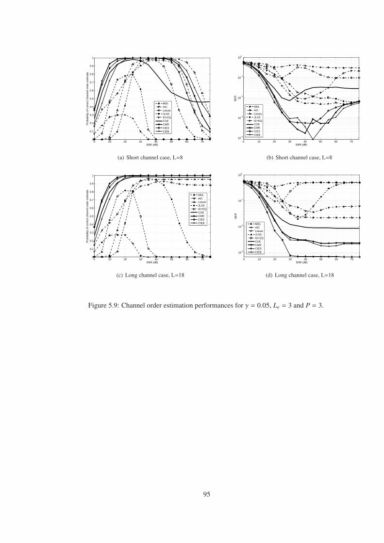
0 10 20 30 40 50 60 700

0.1

0.2

0.3

0.4

0.5

0.6

0.7

0.8

0.9

1

SNR (dB)

Pro

babi

lity

of c

orre

ct c

hann

el o

rder

est

imat

e


(a) Short channel case, L=8

0 10 20 30 40 50 60 7010

−4

10−3

10−2

10−1

100

SNR (dB)

BE

R


(b) Short channel case, L=8

0 10 20 30 40 50 60 700

0.1

0.2

0.3

0.4

0.5

0.6

0.7

0.8

0.9

1

SNR (dB)

Pro

babi

lity

of c

orre

ct c

hann

el o

rder

est

imat

e


(c) Long channel case, L=18

0 10 20 30 40 50 60 70

10−3

10−2

10−1

100

SNR (dB)

BE

R


(d) Long channel case, L=18

Figure 5.9: Channel order estimation performances for γ = 0.05, Le = 3 and P = 3.

95

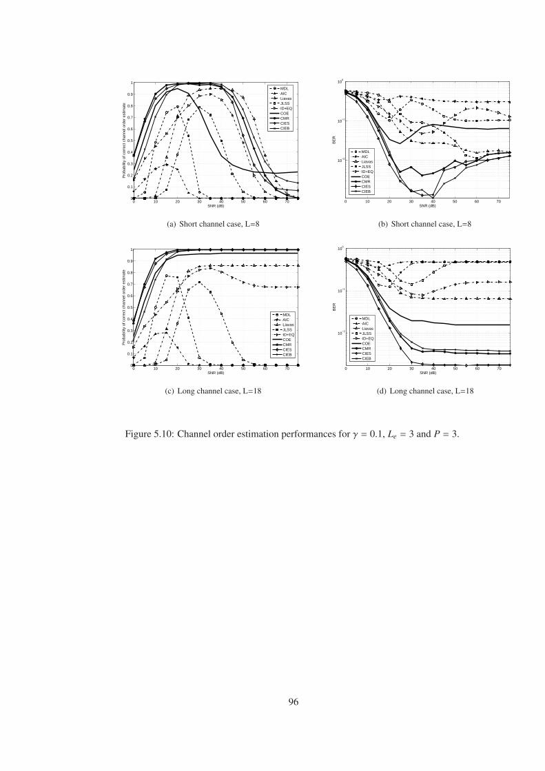
0 10 20 30 40 50 60 700

0.1

0.2

0.3

0.4

0.5

0.6

0.7

0.8

0.9

1

SNR (dB)

Pro

babi

lity

of c

orre

ct c

hann

el o

rder

est

imat

e



0 10 20 30 40 50 60 70

10−2

10−1

100

SNR (dB)

BE

R



0 10 20 30 40 50 60 700

0.1

0.2

0.3

0.4

0.5

0.6

0.7

0.8

0.9

1

SNR (dB)

Pro

babi

lity

of c

orre

ct c

hann

el o

rder

est

imat

e



0 10 20 30 40 50 60 70

10−2

10−1

100

SNR (dB)

BE

R




96

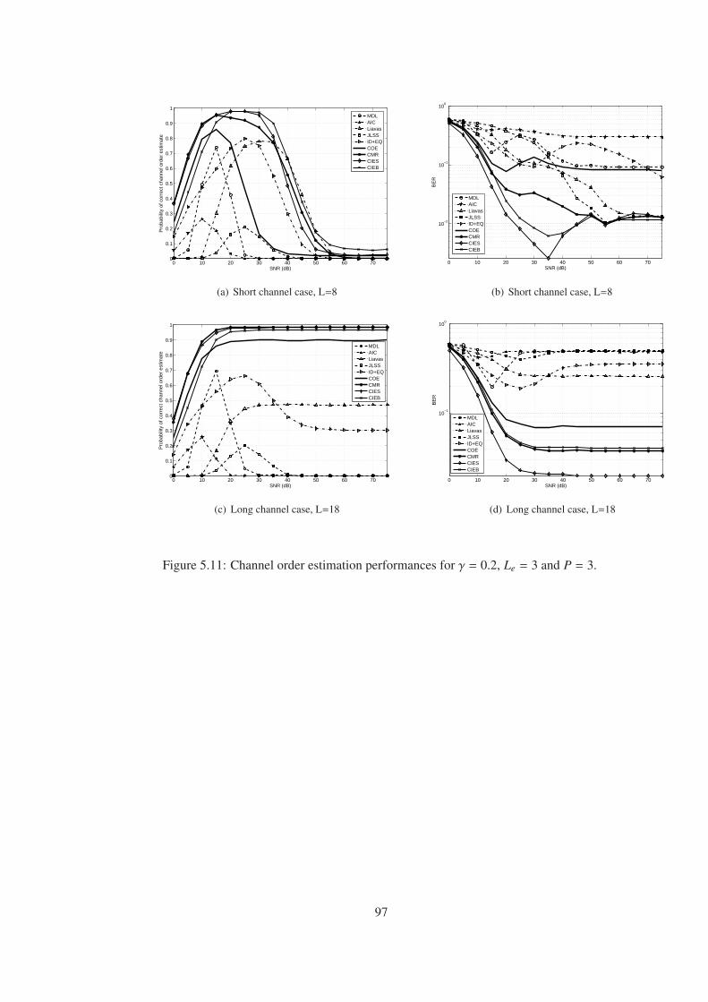
0 10 20 30 40 50 60 700

0.1

0.2

0.3

0.4

0.5

0.6

0.7

0.8

0.9

1

SNR (dB)

Pro

babi

lity

of c

orre

ct c

hann

el o

rder

est

imat

e



0 10 20 30 40 50 60 70

10−2

10−1

100

SNR (dB)

BE

R



0 10 20 30 40 50 60 700

0.1

0.2

0.3

0.4

0.5

0.6

0.7

0.8

0.9

1

SNR (dB)

Pro

babi

lity

of c

orre

ct c

hann

el o

rder

est

imat

e



0 10 20 30 40 50 60 70

10−1

100

SNR (dB)

BE

R




97

5.4 BER When Different Channel Estimation Algorithms are Used

In blind identification, it is possible to use a channel order estimation algorithms which has a

tendency to overestimate like MDL and AIC. Then algorithms robust to overestimation such

as LP [14, 15] and MLP [17] can be employed.

Therefore, correct channel order estimation may not be seen as a critical issue. However

the performance of such algorithms is low compared to deterministic methods such SS [6]

and LSS [7, 3] when the channel order is correctly estimated. On the other hand, SS and

LSS algorithms are not robust to channel order overestimation and their performances are

dramatically reduced when the channel order is not correctly known [22]. With the help

high performance channel order estimator they can be used effectively. Therefore, COE and

CMR can be a solution for this problem. In order to determine the best approach in blind

identification, LP based approach and the proposed blind algorithms are compared by using

extensive simulations. For that purpose LP [14, 15] and MLP [17] algorithms are used as the

algorithms robust to overestimation of the channel order and SS and LSS algorithms are used

as high performance deterministic algorithms in the comparison.

5.4.1 Performance of The Channel Estimation Algorithms in Case of Channel Order

Mismatch

Channel estimation performances of LP, MLP, SS and LSS algorithms are compared in case

of channel order mismatch. The channel given in [15] is used in the simulations. It is a four

channel (P = 4) SIMO channel with channel order L = 5. Channel coefficents are given in

Table 5.1 Length of the input signal is 200 and QPSK is used as a modulation waveform.

500 trials are realized for each simulation and at each trial input signal and channel noise

is randomly generated. When SS and LSS algorithms are used, channel is equalized with

Wiener equalizer. MLP algorithm obtains the inputs signal besides the channel coefficients.

Channel estimation performances is measured by the normalized mean square error (NMSE)

. NMSE is defined as,

NMS E =

Nr∑n=1

∥∥∥hn − h∥∥∥2

Nr ‖h‖2(5.15)

98

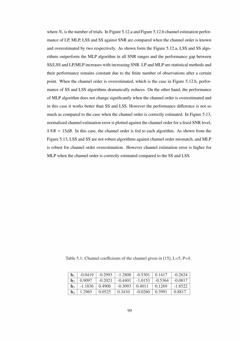
where Nr is the number of trials. In Figure 5.12.a and Figure 5.12.b channel estimation perfor-

mance of LP, MLP, LSS and SS against SNR are compared when the channel order is known

and overestimated by two respectively. As shown form the Figure 5.12.a, LSS and SS algo-

rithms outperform the MLP algorithm in all SNR ranges and the performance gap between

SS/LSS and LP/MLP increases with increasing SNR. LP and MLP are statistical methods and

their performance remains constant due to the finite number of observations after a certain

point. When the channel order is overestimated, which is the case in Figure 5.12.b, perfor-

mance of SS and LSS algorithms dramatically reduces. On the other hand, the performance

of MLP algorithm does not change significantly when the channel order is overestimated and

in this case it works better than SS and LSS. However the performance difference is not so

much as compared to the case when the channel order is correctly estimated. In Figure 5.13,

normalized channel estimation error is plotted against the channel order for a fixed SNR level,

S NR = 15dB. In this case, the channel order is fed to each algorithm. As shown from the

Figure 5.13, LSS and SS are not robust algorithms against channel order mismatch, and MLP

is robust for channel order overestimation. However channel estimation error is higher for

MLP when the channel order is correctly estimated compared to the SS and LSS.

Table 5.1: Channel coefficients of the channel given in [15], L=5, P=4.

h1 -0.0419 -0.2993 -1.2808 -0.5301 0.1417 -0.2624h2 0.9097 -0.2021 -0.4401 -1.0153 -0.5364 -0.0817h3 -1.1836 0.4906 -0.3093 0.4011 0.1269 -1.8522h4 1.2965 0.0525 0.3410 -0.0260 0.3991 0.8817

99

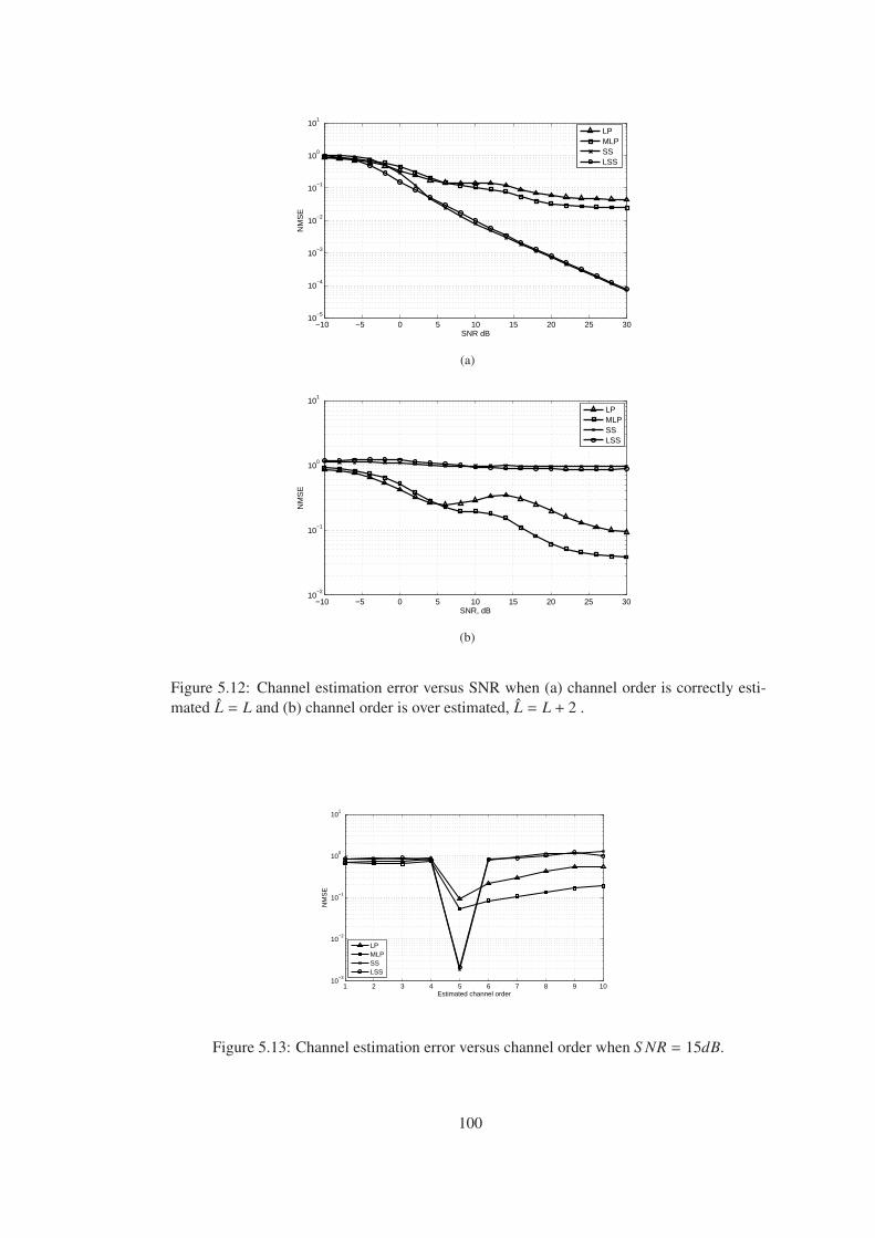
−10 −5 0 5 10 15 20 25 3010

−5

10−4

10−3

10−2

10−1

100

101

SNR dB

NM

SE

LPMLPSSLSS

(a)

−10 −5 0 5 10 15 20 25 3010

−2

10−1

100

101

SNR, dB

NM

SE

LPMLPSSLSS

(b)

Figure 5.12: Channel estimation error versus SNR when (a) channel order is correctly esti-mated L = L and (b) channel order is over estimated, L = L + 2 .

1 2 3 4 5 6 7 8 9 1010

−3

10−2

10−1

100

101


NM

SE

LPMLPSSLSS

Figure 5.13: Channel estimation error versus channel order when S NR = 15dB.

100

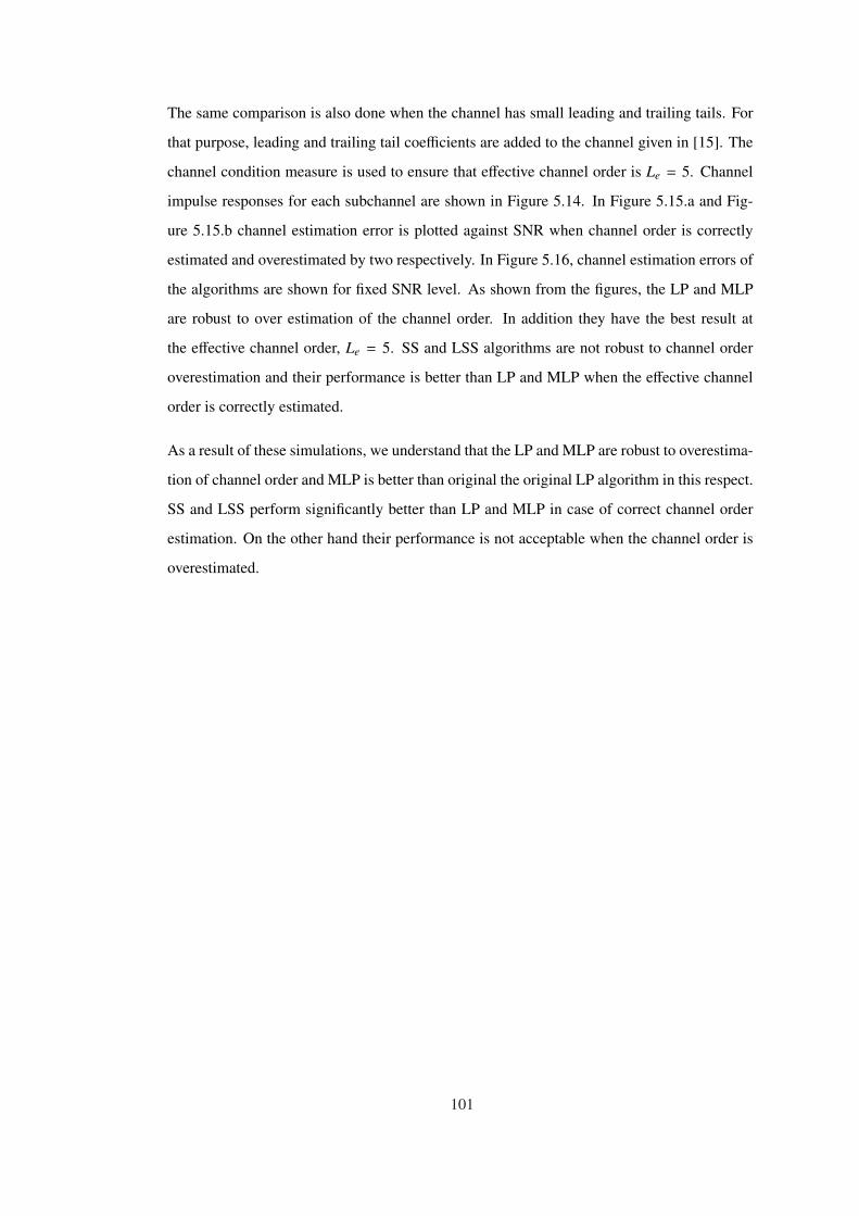
The same comparison is also done when the channel has small leading and trailing tails. For

that purpose, leading and trailing tail coefficients are added to the channel given in [15]. The

channel condition measure is used to ensure that effective channel order is Le = 5. Channel

impulse responses for each subchannel are shown in Figure 5.14. In Figure 5.15.a and Fig-

ure 5.15.b channel estimation error is plotted against SNR when channel order is correctly

estimated and overestimated by two respectively. In Figure 5.16, channel estimation errors of

the algorithms are shown for fixed SNR level. As shown from the figures, the LP and MLP

are robust to over estimation of the channel order. In addition they have the best result at

the effective channel order, Le = 5. SS and LSS algorithms are not robust to channel order

overestimation and their performance is better than LP and MLP when the effective channel

order is correctly estimated.

As a result of these simulations, we understand that the LP and MLP are robust to overestima-

tion of channel order and MLP is better than original the original LP algorithm in this respect.

SS and LSS perform significantly better than LP and MLP in case of correct channel order

estimation. On the other hand their performance is not acceptable when the channel order is

overestimated.

101

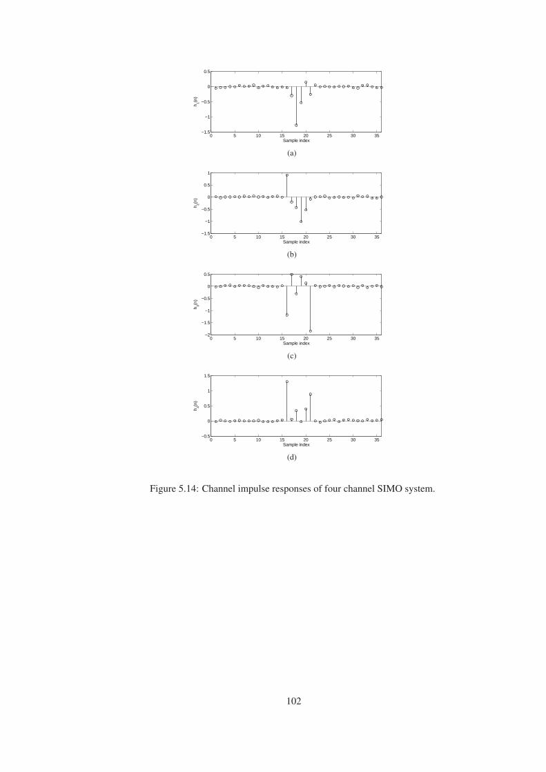
0 5 10 15 20 25 30 35−1.5

−1

−0.5

0

0.5

Sample index

h 1(n)

(a)

0 5 10 15 20 25 30 35−1.5

−1

−0.5

0

0.5

1

Sample index

h 2(n)

(b)

0 5 10 15 20 25 30 35−2

−1.5

−1

−0.5

0

0.5

Sample index

h 3(n)

(c)

0 5 10 15 20 25 30 35−0.5

0

0.5

1

1.5

Sample index

h 4(n)

(d)

Figure 5.14: Channel impulse responses of four channel SIMO system.

102

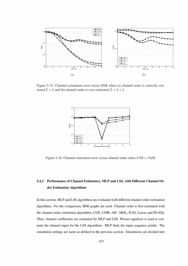
−10 −5 0 5 10 15 20 25 3010

−3

10−2

10−1

100

SNR, dB

NM

SE

MLPLSSSSLP

(a)

−10 −5 0 5 10 15 20 25 3010

−2

10−1

100

SNR, dB

NM

SE

MLPLSSSSLP

(b)

Figure 5.15: Channel estimation error versus SNR when (a) channel order is correctly esti-mated L = L and (b) channel order is over estimated, L = L + 2 .

1 2 3 4 5 6 7 8 910

−3

10−2

10−1

100

101


NM

SE

LPMLPSSLSS

Figure 5.16: Channel estimation error versus channel order when S NR = 15dB.

5.4.2 Performance of Channel Estimators, MLP and LSS, with Different Channel Or-

der Estimation Algorithms

In this section, MLP and LSS algorithms are evaluated with different channel order estimation

algorithms. For the comparison, BER graphs are used. Channel order is first estimated with

the channel order estimation algorithms, COE, CMR, AIC, MDL, JLSS, Liavas and ID+EQ.

Then, channel coefficients are estimated by MLP and LSS. Wiener equalizer is used to esti-

mate the channel input for the LSS algorithms. MLP finds the input sequence jointly. The

simulation settings are same as defined in the previous section. Simulations are divided into

103

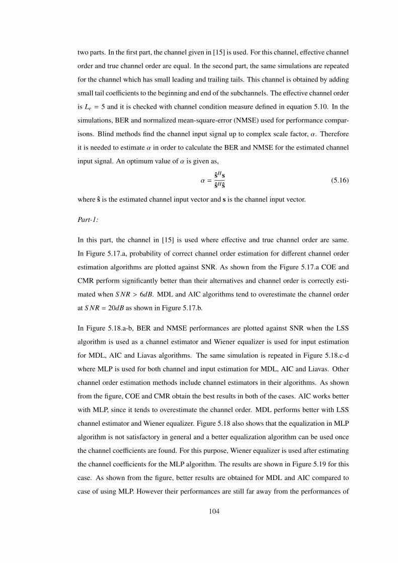
two parts. In the first part, the channel given in [15] is used. For this channel, effective channel

order and true channel order are equal. In the second part, the same simulations are repeated

for the channel which has small leading and trailing tails. This channel is obtained by adding

small tail coefficients to the beginning and end of the subchannels. The effective channel order

is Le = 5 and it is checked with channel condition measure defined in equation 5.10. In the

simulations, BER and normalized mean-square-error (NMSE) used for performance compar-

isons. Blind methods find the channel input signal up to complex scale factor, α. Therefore

it is needed to estimate α in order to calculate the BER and NMSE for the estimated channel

input signal. An optimum value of α is given as,

α =sHssH s

(5.16)

where s is the estimated channel input vector and s is the channel input vector.

Part-1:

In this part, the channel in [15] is used where effective and true channel order are same.

In Figure 5.17.a, probability of correct channel order estimation for different channel order

estimation algorithms are plotted against SNR. As shown from the Figure 5.17.a COE and

CMR perform significantly better than their alternatives and channel order is correctly esti-

mated when S NR > 6dB. MDL and AIC algorithms tend to overestimate the channel order

at S NR = 20dB as shown in Figure 5.17.b.

In Figure 5.18.a-b, BER and NMSE performances are plotted against SNR when the LSS

algorithm is used as a channel estimator and Wiener equalizer is used for input estimation

for MDL, AIC and Liavas algorithms. The same simulation is repeated in Figure 5.18.c-d

where MLP is used for both channel and input estimation for MDL, AIC and Liavas. Other

channel order estimation methods include channel estimators in their algorithms. As shown

from the figure, COE and CMR obtain the best results in both of the cases. AIC works better

with MLP, since it tends to overestimate the channel order. MDL performs better with LSS

channel estimator and Wiener equalizer. Figure 5.18 also shows that the equalization in MLP

algorithm is not satisfactory in general and a better equalization algorithm can be used once

the channel coefficients are found. For this purpose, Wiener equalizer is used after estimating

the channel coefficients for the MLP algorithm. The results are shown in Figure 5.19 for this

case. As shown from the figure, better results are obtained for MDL and AIC compared to

case of using MLP. However their performances are still far away from the performances of

104

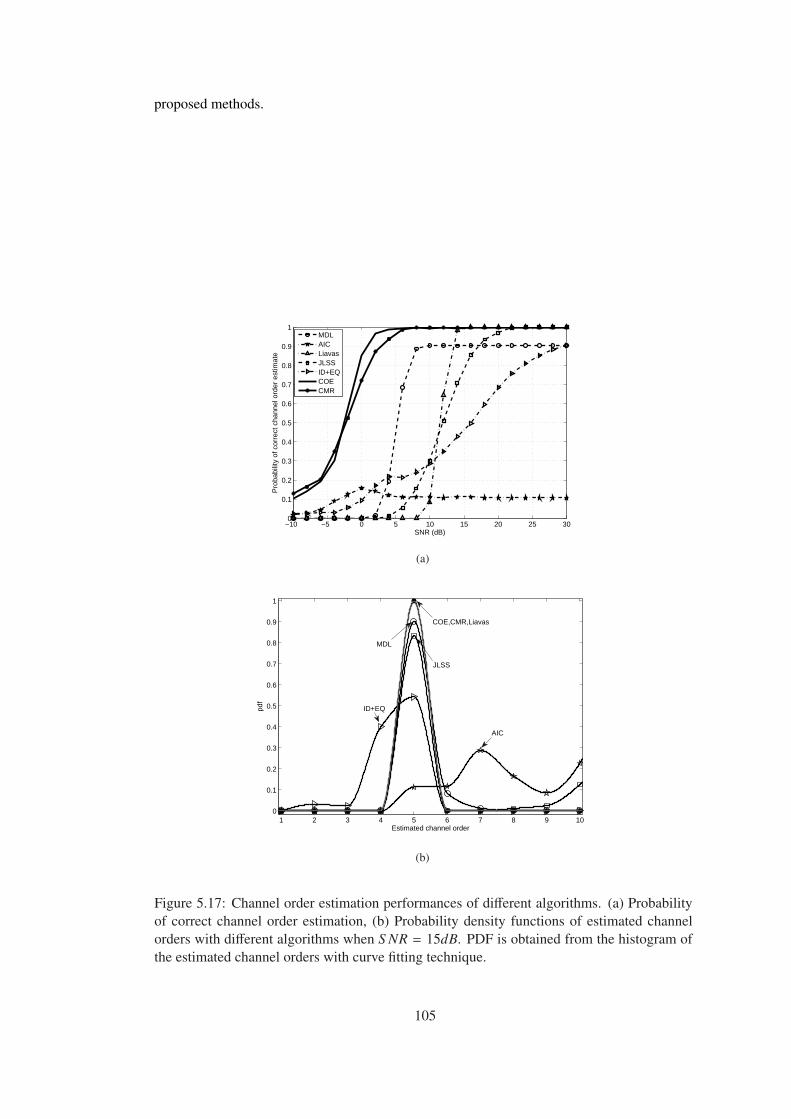
proposed methods.

−10 −5 0 5 10 15 20 25 300

0.1

0.2

0.3

0.4

0.5

0.6

0.7

0.8

0.9

1

SNR (dB)

Pro

babi

lity

of c

orre

ct c

hann

el o

rder

est

imat

e


(a)

1 2 3 4 5 6 7 8 9 100

0.1

0.2

0.3

0.4

0.5

0.6

0.7

0.8

0.9

1


pdf

COE,CMR,Liavas

JLSS

MDL

ID+EQ

AIC

(b)

Figure 5.17: Channel order estimation performances of different algorithms. (a) Probabilityof correct channel order estimation, (b) Probability density functions of estimated channelorders with different algorithms when S NR = 15dB. PDF is obtained from the histogram ofthe estimated channel orders with curve fitting technique.

105

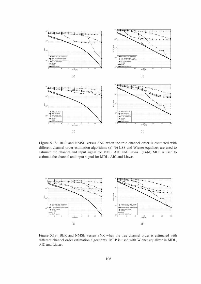
0 2 4 6 8 10 12 14 16

10−3

10−2

10−1

100

SNR (dB)

BE

R

MDL with LSS and WienerAIC with LSS and WienerLiavas with LSS and WienerJLSS with WienerID+EQCOECMR Wiener

(a)

0 5 10 15 20 25 3010

−4

10−3

10−2

10−1

100

SNR (dB)

INP

UT

NM

SE

MDL with LSS and WienerAIC with LSS and WienerLiavas with LSS and WienerJLSS with WienerID+EQCOECMR with Wiener

(b)

0 2 4 6 8 10 12 14 16

10−3

10−2

10−1

100

SNR (dB)

BE

R

MDL with MLPAIC with MLPLiavas with MLPJLSS with WienerID+EQCOECMR with Wiener

(c)

0 5 10 15 20 25 3010

−4

10−3

10−2

10−1

100

SNR (dB)

INP

UT

NM

SE

MDL with MLPAIC with MLPLiavas with MLPJLSS with WienerID+EQCOECMR Wiener

(d)

Figure 5.18: BER and NMSE versus SNR when the true channel order is estimated withdifferent channel order estimation algorithms (a)-(b) LSS and Wiener equalizer are used toestimate the channel and input signal for MDL, AIC and Liavas. (c)-(d) MLP is used toestimate the channel and input signal for MDL, AIC and Liavas.

0 2 4 6 8 10 12 14 16

10−3

10−2

10−1

100

SNR (dB)

BE

R

MDL with MLP and WienerAIC with MLP and WienerLiavas with MLP and WienerJLSS WienerID+EQ COE CMR Wiener

(a)

0 5 10 15 20 25 3010

−4

10−3

10−2

10−1

100

SNR (dB)

INP

UT

NM

SE

MDL with MLP and WienerAIC with MLP and WienerLiavas with MLP and WienerJLSS with WienerID+EQCOECMR with Wiener

(b)

Figure 5.19: BER and NMSE versus SNR when the true channel order is estimated withdifferent channel order estimation algorithms. MLP is used with Wiener equalizer in MDL,AIC and Liavas.

106

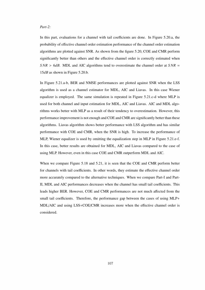
Part-2:

In this part, evaluations for a channel with tail coefficients are done. In Figure 5.20.a, the

probability of effective channel order estimation performance of the channel order estimation

algorithms are plotted against SNR. As shown from the figure 5.20, COE and CMR perform

significantly better than others and the effective channel order is correctly estimated when

S NR > 6dB. MDL and AIC algorithms tend to overestimate the channel order at S NR =

15dB as shown in Figure 5.20.b.

In Figure 5.21.a-b, BER and NMSE performances are plotted against SNR when the LSS

algorithm is used as a channel estimator for MDL, AIC and Liavas. In this case Wiener

equalizer is employed. The same simulation is repeated in Figure 5.21.c-d where MLP is

used for both channel and input estimation for MDL, AIC and Liavas. AIC and MDL algo-

rithms works better with MLP as a result of their tendency to overestimation. However, this

performance improvement is not enough and COE and CMR are significantly better than these

algorithms. Liavas algorithm shows better performance with LSS algorithm and has similar

performance with COE and CMR, when the SNR is high. To increase the performance of

MLP, Wiener equalizer is used by omitting the equalization step in MLP in Figure 5.21.e-f.

In this case, better results are obtained for MDL, AIC and Liavas compared to the case of

using MLP. However, even in this case COE and CMR outperform MDL and AIC.

When we compare Figure 5.18 and 5.21, it is seen that the COE and CMR perform better

for channels with tail coefficients. In other words, they estimate the effective channel order

more accurately compared to the alternative techniques. When we compare Part-I and Part-

II, MDL and AIC performances decreases when the channel has small tail coefficients. This

leads higher BER. However, COE and CMR performances are not much affected from the

small tail coefficients. Therefore, the performance gap between the cases of using MLP+

MDL/AIC and using LSS+COE/CMR increases more when the effective channel order is

considered.

107

−10 −5 0 5 10 15 20 25 300

0.1

0.2

0.3

0.4

0.5

0.6

0.7

0.8

0.9

1

SNR (dB)

Pro

babi

lity

of c

orre

ct c

hann

el o

rder

est

imat

e


(a)

1 2 3 4 5 6 7 8 9 100

0.1

0.2

0.3

0.4

0.5

0.6

0.7

0.8

0.9

1

Estimated Channel Order

pdf

COE, CMR, Liavas

MDL

JLSS

ID+EQAIC

(b)

Figure 5.20: Channel order estimation performances of different algorithms. (a) Probabilityof correct channel order estimation, (b) Probability density functions of estimated channelorders with different algorithms when S NR = 15dB. PDF is obtained from the histogram ofthe estimated channel orders with curve fitting technique.

108

0 2 4 6 8 10 12 14 16 18

10−4

10−3

10−2

10−1

100

SNR (dB)

BE

R


(a)

0 5 10 15 20 25 3010

−3

10−2

10−1

100

SNR (dB)

INP

UT

NM

SE


(b)

0 2 4 6 8 10 12 14 16 18

10−4

10−3

10−2

10−1

100

SNR (dB)

BE

R


(c)

0 5 10 15 20 25 3010

−3

10−2

10−1

100

SNR (dB)

INP

UT

NM

SE


(d)

0 2 4 6 8 10 12 14 16

10−4

10−3

10−2

10−1

100

SNR (dB)

BE

R


(e)

0 5 10 15 20 25 3010

−3

10−2

10−1

100

SNR (dB)

INP

UT

NM

SE


(f)

Figure 5.21: BER and NMSE versus SNR when the effective channel order is estimated withdifferent channel order estimation algorithms (a)-(b) LSS and Wiener equalizer are used toestimate the channel and input signal for MDL, AIC and Liavas. (c)-(d) MLP is used toestimate the channel and input signal for MDL, AIC and Liavas. (e)-(f) MLP is used withWiener equalizer in MDL, AIC and Liavas.

109

5.5 Performance Comparison of Proposed Methods with DFE in Fractionally

Spaced SISO Channels

In SISO systems, equalizer performance can be significantly improved by introducing nonlin-

earity into the equalizer structure [41, 45]. One of the best example of nonlinear equalizers is

the decision feed back equalizer (DFE) [45]. The nonlinearity of DFE comes from the nonlin-

ear characteristics of the detector that provides an input to the feedback filter. The main idea is

that if the previously detected symbols are known, the ISI introduced on the currents symbol

can be removed by the subtraction of previously detected symbols with appropriate weight-

ing [41]. The advantage of DFE over linear equalizer is the feedback filter which removes

residual ISI after feedforward filter. DFE feedback loop remains stable as long as correct

decisions are done at the decision ruler (or slicer). If an error occurs at the decision, the DFE

starts generating errors on the equalized signal, and it cause more decision errors and hence

error propagation. This is the main drawback of DFE systems. The convergence problem

is another drawback of the algorithm especially for time varying channels. In this case, for

fast convergence, training data should be repeated occasionally. Training based DFE system

starts in training mode. After the filter coefficients converged, it switches to decision directed

mode. For proper operation of decision directed mode, eye diagram of the signal at decision

input should be sufficiently open. Training sequence is used to open the eye diagram. Blind

methods can also be used for this purpose. Constant Modulus Algorithm (CMA) (or Godard)

method [30] is one of the most popular blind methods used with DFE.

DFE is a suboptimum method considering that it assumes that past decision are correct. The

optimum solution is the maximum likelihood sequence estimator (MLSE). If the feedforward

filter were infinitely long, DFE would be a perfect zero-forcing equalizer.

Fractionally spaced equalization is used to provide immunity to sampling errors. Fractionally

spaced system corresponds to oversampling of the received signal. This receiving structure

can also be implemented by a SIMO system by means of using a polyphase structure. There-

fore, blind methods proposed for SIMO systems can be used in this system structure. In SIMO

systems, perfect identification and equalization is possible with the help deterministic blind

methods such as SS, CR, and LSS. In practice, blind deterministic methods are not preferred

due to their computational complexity and the lack of robustness to channel order. In this the-

sis, COE and CMR are proposed to solve the robustness problem. In turns out that proposed

110

blind approach performs better in case of blind problem setting. To verify this, we have com-

pared the DFE method with the proposed methods, COE and CMR, for oversampled SISO

channels. In the simulations, the channel given in [15] used. For this channel, oversampling

ratio is 4 and the channel order is L = 5. QPSK is used as modulation waveform and the

length of the transmitted data is 1000. Fractionally spaced DFE with constant modulus algo-

rithm and DFE with training are compared with the channel order estimation methods COE

and CMR. In CMR, channel is equalized with Wiener equalizer. DFE uses 25 tap feedforward

filter and two tap feedback filter; the step size is 0.0005. 500 trials are used in the simulations.

The result of DFE is compared after it is converged. In training based DFE first 500 samples

are used for training purpose and recursive least squares (RLS) algorithm is used to update

filter coefficient with a forgetting factor of 0.98. Note that DFE with training is considered

only to see the performance in comparison. Since other techniques are completely blind and

do not take advantage of training sequence.

In Figure 5.22.a and Figure 5.22.b, MSE and BER performance of the algorithms are pre-

sented. As shown from the figures, proposed methods, COE and CMR perform significantly

better than DFE with CMA especially at high SNR ranges, due to the accuracy in channel

order estimation and finite convergence of the LSS algorithm. On the other hand, the perfor-

mance of DFE with training is close to the COE and CMR but not better. In Figure 5.23.a and

Figure 5.23.b, BER and MSE performance of the algorithms are presented, when the channel

includes long tail coefficients. Transfer functions of the channels are given in Figure 5.14. As

shown from Figure 5.23.a-b,, the similar results are obtained in case of a channel with tails.

In Figure 5.24, performance of the algorithms are tested with the microwave channel given

in ”http://spib.rice.edu/spib/microwave.html” as chan3.mat, whose impulse response is plotted

in Figure 5.3. As shown from the figures, DFE with training shows the best performance.

However, CME and CMR are still better than the blind DFE significantly. The microwave

channel has two taps per channel, and DFE can estimate the true equalizer coefficients better

using the same number of filter coefficients. On the other hand COE and CMR performances

decrease when the number of channels in SIMO system is decreased.

111

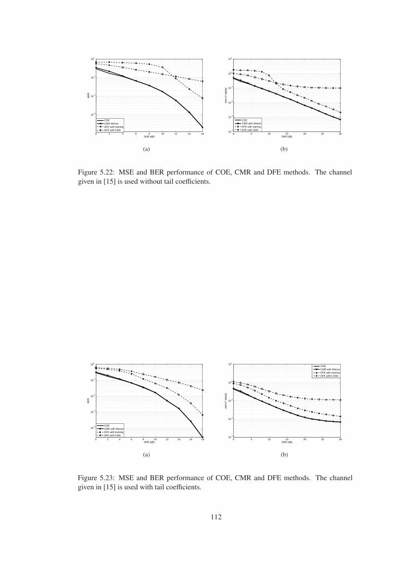
0 2 4 6 8 10 12 14 16

10−3

10−2

10−1

100

SNR (dB)

BE

R

COECMR WienerDFE with trainingDFE with CMA

(a)

0 5 10 15 20 25 3010

−4

10−3

10−2

10−1

100

101

SNR (dB)

INP

UT

NM

SE

COECMR with WienerDFE with trainingDFE with CMA

(b)

Figure 5.22: MSE and BER performance of COE, CMR and DFE methods. The channelgiven in [15] is used without tail coefficients.

0 2 4 6 8 10 12 14 16 18

10−4

10−3

10−2

10−1

100

SNR (dB)

BE

R

COECMR with WienerDFE with trainingDFE with CMA

(a)

0 5 10 15 20 25 3010

−3

10−2

10−1

100

101

SNR (dB)

INP

UT

NM

SE

COECMR with WienerDFE with trainingDFE withn CMA

(b)

Figure 5.23: MSE and BER performance of COE, CMR and DFE methods. The channelgiven in [15] is used with tail coefficients.

112

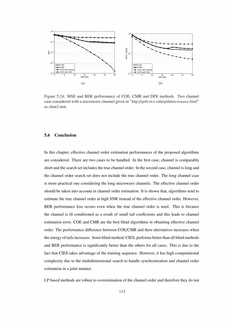
0 5 10 15 20 25 3010

−4

10−3

10−2

10−1

100

SNR (dB)

BE

R

COECMRDFE with trainingDFE with CMA

(a)

0 5 10 15 20 25 3010

−2

10−1

100

SNR (dB)

INP

UT

NM

SE

COECMRDFE with trainingDFE with CMA

(b)

Figure 5.24: MSE and BER performance of COE, CMR and DFE methods. Two channelcase considered with a microwave channel given in ”http://spib.rice.edu/spib/microwave.html”as chan3.mat.

5.6 Conclusion

In this chapter, effective channel order estimation performances of the proposed algorithms

are considered. There are two cases to be handled. In the first case, channel is comparably

short and the search set includes the true channel order. In the second case, channel is long and

the channel order search set does not include the true channel order. The long channel case

is more practical one considering the long microwave channels. The effective channel order

should be taken into account in channel order estimation. It is shown that, algorithms tend to

estimate the true channel order at high SNR instead of the effective channel order. However,

BER performance loss occurs even when the true channel order is used. This is because

the channel is ill conditioned as a result of small tail coefficients and this leads to channel

estimation error. COE and CMR are the best blind algorithms in obtaining effective channel

order. The performance difference between COE/CMR and their alternatives increases when

the energy of tails increases. Semi-blind method, CIES, performs better than all blind methods

and BER performance is significantly better than the others for all cases. This is due to the

fact that CIES takes advantage of the training sequence. However, it has high computational

complexity due to the multidimensional search to handle synchronization and channel order

estimation in a joint manner.

LP based methods are robust to overestimation of the channel order and therefore they do not

113

require high performance channel order estimators. On the other hand, it is seen that their

performances are not good as the deterministic channel estimation methods such as SS and

LSS when the channel order is correctly estimated. SS and LSS require correct channel order

estimation to work well. COE and CMR have superior channel order estimation performance

and the robustness problem of the SS and LSS algorithms for channel order overestimation

is handled by using COE and CMR. Much better BER is obtained by using COE and CMR

with LSS compared to the case of using LP based algorithm as a channel estimator. COE and

CMR are investigated with the LSS algorithm in order to estimate channel coefficients. LSS

algorithm has certain properties which make it ideal choice in order estimation. Proposed

methods are also compared with DFE, which does not require channel order, in a fractional

spaced SISO systems. It is shown that COE and CMR outperform blind DFE especially at

high SNR ranges. On the other hand, DFE with training shows better performance than COE

and CMR with the loss in bandwidth efficiency, when the number of channels is small.

114

CHAPTER 6

CONCLUSION

Blind system identification is an important topic in signal processing with many applications

in different fields including communications, radar, acoustics, speech and more. The main

problem in this context is to find the system impulse response and the input by using only

the output samples. This problem can be considered in SISO, SIMO and MIMO systems. In

SISO systems, there are techniques which can solve the blind identification problem under

certain conditions [30, 42, 43]. In SIMO systems, blind identification problem is shown to

be solvable with fewer constraints. In addition, it is possible to solve the problem perfectly

in noise free case, when there is no common channel zero between subchannels of SIMO

system. The problem in MIMO setting is the hardest one to solve due to many reasons.

In this thesis, blind channel order estimation problem is considered for SIMO communication

systems. While the importance of the estimation and use of channel order is widely known in

signal processing community, this thesis shows that the implications of the effective channel

order estimation are more significant than the common expectations.

In this thesis, two new blind channel order estimation algorithms are presented, namely COE

and CMR. These algorithms are proved to have the finite convergence property, i.e., they

are guaranteed to find the true channel order from finite number of observations for noise

free case. Previously there were only two algorithms known in the literature with the same

property. Proposed algorithms work in completely different ways but their cost functions have

similarities. In fact, they have a ”convex like” shape which allows one to pick the channel

order corresponding to the minimum value of the cost function. Therefore there is no need

to define and use a threshold value. COE algorithm is based on the estimation of channel

output. The difference between the estimated and observed channel outputs is taken as the cost

115

function. In estimating the channel output, LSS algorithm as a channel estimator and Wiener

equalizer are used. The superior performance of the COE method on estimating the channel

order is based on the properties of LSS algorithms which are derived in this thesis. It is shown

that the LSS algorithm generates common channel zeros besides the true channel zeros in

noise free case when the order is overestimated. Furthermore, these common zeros are located

close to the unit circle. When the common channel zeros are located on the unit circle, the

inverse channel transfer function does not decay to zero rapidly. Perfect FIR equalization is

not possible, and equalization error is large. Therefore equalization error is higher for the

LSS case when the channel order is overestimated. The convex like cost function of COE is

much deeper compared to the case where other blind estimators such as SS and CR are used.

CMR method also uses the LSS algorithm. It is based on generating a relation in terms of the

channel matrix. It turns out that the channel matrix relation is established by a matrix which

has a Toeplitz structure only if the channel order is overestimated by one. The deviation from

the Toeplitz structure is used to obtain a cost function for the channel order estimation. The

estimation of common channel zeros requires the inverse of the estimated channel matrix.

When the channel matrix includes common channel zeros positioned on the unit circle, the

deviation from the Toeplitz structure increases and a convex like function with a deeper valley

at the true channel order is obtained. It should also be noted that the common channel zeros

found by the LSS algorithm has no relation to the input or channel in general.

While the finite sample convergence property is important, the performance of the order

estimation algorithms for noisy observations is critical. Especially when the channel filter

has some leading and trailing tails, estimation of the effective channel order rather than the

true channel order becomes important. Deterministic channel estimation methods require the

knowledge of the channel order. In the case of the small tail coefficients, channel identifica-

tion is more problematic due to the reason that tail coefficients have the effect of colored noise

on the channel. In [47] the condition measure is defined for the calculation of the effective

channel order for a given channel. It also measures the degree of the ill conditioning of the

channel. Estimation of effective channel order is important to obtain the best performance in

blind channel identification. Proposed methods are tested with channels having small leading

and trailing tails. In the simulations, randomly generated channels as well as measured mi-

crowave channels are used for complete evaluation. COE and CMR shows significantly better

performance in estimating the effective channel order in a wide SNR range. When COE and

116

CMR are compared, CMR is slightly better than COE for order estimation. However this

difference leads to considerable BER difference, since LSS method is not robust to over or

under estimation of the channel order. Proposed algorithms are robust to different parameters

such as the number of channels, channel order and the number of input samples. Hence, they

are applicable for the applications having different receiver settings and channel conditions.

Proposed methods COE and CMR use the LSS algorithm which is integrated to the channel

order estimation. Therefore these two algorithms estimate the channel coefficients in a joint

manner. Since LSS is one of the best channel estimator, the combination performs well in

blind identification.

The research on blind channel order estimation and system identification can be grouped

in two main categories. In the first group, there is a significant amount of work devoted

to the estimation of true and/or effective channel order. In the second group, there is an

alternative approach where it is sufficient to have a rough idea about the channel in order to

have an overestimated channel order. The leading technique in this group is the blind channel

equalization and estimation by linear prediction. While these two approaches are alternatives

of each other, none of the previous works compare these two approaches in order to have a

good idea about the best possible technique for blind channel order estimation. It is believed

that this thesis sheds a light on these alternative techniques by comparing them for a variety

of cases.

LP based methods are claimed to be robust to overestimation of channel order. This property

makes them popular in the solution of channel equalization problem when the channel order

is not exactly known. LP method is first proposed by Slock [14],and it is based on the fact that

moving average (MA) SIMO channel output can also be represented as an AR process, whose

innovation is the SIMO channel input. LP is originally developed by assuming that the first

channel coefficient is different from zero [14]. It is known that if this condition is not satisfied

and h(0) is close to zero, prediction error increases. In [17], this problem is solved to a certain

extend. LP algorithm uses statistical characteristic of the inputs and it is based on the second

order statistics. It assumes that, the channel input signal is Gaussian distributed white signal

which is not perfectly satisfied in practical applications. Therefore it is not a deterministic

algorithm as opposed to SS, CR and LSS algorithms. Being a non-deterministic method is

the main disadvantage of the LP algorithm, since it is not possible to obtain channel input or

117

channel coefficients without error even in noise free case. LP channel/input estimation error

increases as the overestimation increases. While this increase is relatively small compared to

LSS, SS and CR, LP has the best performance at true or effective channel order. LP can be

considered as a robust algorithm for overestimation, but its equalization performance is poor.

If Wiener equalizer is used instead of its known equalizer, performance can be improved.

Even so it is still much worse than the CMR and COE techniques. As a result, using AIC

or MDL for channel order estimation and LP for channel estimation and equalization does

perform poorly compared to the proposed methods COE and CMR. This shows the value

of accurate channel order estimation. In this respect, the best performance in blind channel

and input estimation can be obtained by the proposed techniques in case of unknown channel

order.

SIMO systems can be obtained in different ways. In one case, SIMO system is obtained by

employing single transmit, multiple receive antennas. In the second case, the SISO system

output is oversampled and polyphase structure is used to obtain the SIMO system. Many com-

munication systems are in SISO structure. They use either symbol rate equalizers or fraction-

ally spaced equalizers. It is known that if there is unknown channel filter, best performance is

obtained by employing a fractionally spaced equalizer [44]. In this case, it is possible to obtain

an equivalent SIMO system. In this thesis, blind decision feedback equalizer for fractionally

spaced equalizer is shown to perform worse than the SIMO system equalization by employing

the proposed techniques even when the comparison is done after DFE is converged. Obvi-

ously the above result is achieved when there is no common zeros for the equivalent SIMO

system. However, it should also be pointed that proposed technique is relatively robust to

closely spaced channel zeros compared to the alternative techniques.

Training sequences are widely used in traditional communication systems for the purpose of

channel equalization and synchronization. With the help of training sequence, channel can be

identified more accurately without any restriction on the channel. However their bandwidth

efficiency is less than the blind methods and requires synchronization for channel identifica-

tion. The number of training samples required for the channel identification depends on the

channel length, therefore at least an upper bound is required for the estimation of the chan-

nel. The best performance is obtained when the channel order is known. Synchronization

is another problem to be solved for training based methods. The use of training sequence in

channel identification requires knowledge of the location of training sequence in the received

118

data stream. Therefore synchronization should be achieved before channel identification or

synchronization and channel estimation problems should be solved in a simultaneous way as

in [34]. To our knowledge, there is no previous work which consider the semi-blind chan-

nel order estimation, channel estimation and synchronization problems simultaneously in the

literature. Channel order is mostly assumed to be known or an upper limit for the chan-

nel order is used. The upper limit for channel order is estimated by MDL or AIC methods

which mostly overestimate the channel order. Recognizing that the best performance can be

achieved with correct channel order estimation, there is a need of channel order estimation

algorithm with high accuracy. For this purpose, blind methods COE and CMR can be used

without the need for the synchronization. In this thesis, semi-blind methods are presented

in order to obtain performance improvement over CMR and COE. In this respect, two new

channel order estimation algorithms, CIES and CIEB, are proposed. CIES and CIEB are

based on the cost function which is obtained by taking the difference of the estimated input

training sequence and known training sequence. The cost function has global minimum at the

true channel order. The difference between two semi-blind methods is due to how they esti-

mate the channel input. In CIEB, blind channel estimation algorithm LSS is used. In CIES,

semi-blind channel estimation method, which is the combination of LSS and training based

least squares method (LST). Semi-blind channel estimation methods combine the advantages

of blind and training only methods and have better performance than blind and training only

methods. Therefore, it is not surprise that CIES perform better than CIEB. However, CIES

has large computational complexity due to multidimensional search to achieve synchroniza-

tion and channel order estimation jointly. Several simulations are done for the performance

comparisons. CIES and CIEB have similar performance with COE and CMR in true and

effective channel order estimation. No improvement is obtained in this respect. However,

CIES has better BER performance than other methods, due to the reason that it uses semi-

blind channel estimator, which estimates the channel more accurately. As a result, semi-blind

method CIES can achieve better BER performance with a loss in bandwidth efficiency and

increase in computational complexity.

119

REFERENCES

[1] L. Tong, G. Xu, and T. Kailath, A new approach to blind identification and equalizationof multipath channel, Proc. of the 25th Asilomar Conference on Signals, Systems, andComputers, Pacific Grove, CA, pp. 856 − 860, November 1991.

[2] Elisabeth de Carvalho, Dirk T. M. Slock, Blind and semi-blind FIR Multichannel Esti-mation: (global) identifiability conditions, IEEE Trans. on Signal Proc., Vol.52, No.4,pp. 1053 − 1064, April 2004.

[3] L. Tong and Q. Zhao, Joint order detection and blind channel estimation by least squaressmoothing, IEEE Trans. on Signal Proc., Vol. 47, pp. 2345 − 2355, Sept. 1999.

[4] A. P. Liavas, P. A. Regalia, On the behaviour of information theoretic criteria for modelorder selection, IEEE Trans. on Signal Proc., Vol. 49, No. 8, pp. 1689 − 1695, Aug.2001.

[5] A.P. Liavas, P.A. Regalia, J.-P. Delmas, Blind channel approximation: effective channelorder determination, IEEE Trans on Signal Proc., Vol. 47, No.12, pp. 3336 − 3344,December 1999.

[6] E. Moulines, P. Duhamel, J. Cardoso, and S. Mayrargue, Subspace methods for blindidentification of multichannel FIR filters, IEEE Trans. on Signal Proc., SP-43(2):516-525, February 1995.

[7] L. Tong and Q. Zhao, ”Blind channel estimation by least squares smoothing,” in Proc.Int. Conf. Acoust. Speech Signal Process., Seattle, vol. IV, pp. 2121 − 2124, WA, 1998.

[8] G. Xu, H. Liu, L. Tong and T. Kailath, A least-squares approach to blind channel iden-tification, IEEE Trans. on Signal Proc., Vol. 43, pp. 2982 − 2993, Dec 1995.

[9] A. Scaglione, G. B. Giannakis, S. Barbarossa, Redundant filterbank precoders andequalizers Part I : Unification and optimum design, IEEE Trans on Signal Processing,vol.47, pp. 1988-2006, Jul. 1999.

[10] A. Scaglione, G. B. Giannakis, S. Barbarossa, Redundant filterbank precoders andequalizers Part II : Blind channel estimation, syncronization and direct equalization,IEEE Trans on Signal Processing, vol.47, pp. 2007 − 2042, Jul.1999.

[11] S. Barbarossa, A. Scaglione, G. B. Giannakis, Performance analysis of a deterministicchannel estimator for block transmission systems with null guard intervals, IEEE Transon Signal Processing, vol.50, pp. 684 − 695, Mar. 2002.

[12] B. Muquet, Wang Zhengdao, G. B. Giannakis, M. de Courville, P: Duhamel, Cyclic Pre-fixing or zero padding for wireless multicarrier transmission?, IEEE Trans. Commun.,vol. 50, pp. 2136 − 2148, Dec. 2002.

120

[13] Georgios B. Giannakis, Cihan Tepedenlioglu, Direct blind equalizers of multiple FIRchannels: A deterministic approach., IEEE Trans. on Signal Proc., Vol.47, No.1, pp.62 − 74, Jan. 1999.

[14] D. Slock, Blind fractionally-spaced equalization, perfect-reconstruction filter banks andmultichannel linear prediction, Proc. IEEE ICASSP Conf., Adalaide, Australia, pp.IV/585 − IV/588, Apr. 1994.

[15] K. Abed-Meraim, R. Moulines, and P. Loubaton, Prediction error method for secondorder blind identification, IEEE Trans. Signal Proc., Vol.45, pp. 694 − 705, Mar. 1997.

[16] Houcem Gazzah, Phillip A. Regalia, Jean-Pierre Delmas, and Karim Abed-Meraim,ABlind Multichannel Identification Algorithm Robust to Order Overestimation, IEEETrans. on Signal Processing, vol.50, no. 6, pp. 1449 − 1458, June 2002.

[17] Houcem Gazzah, Optimum blind multichannel equalization using the linear predictionalgorithm, IEEE Trans. on Signal Processing, vol.54, no. 8, pp. 3242−3247, June 2006.

[18] A. Gorokhov and P. Loubaton, Blind identification of MIMO-FIR systems: A generalizedprediction approach, Signal Process., vol. 73, pp. 105 − 124, 1999.

[19] J. Rissanen, Modelling by shortest data description Automatica, Vol.14, pp. 465 − 471,1978.

[20] H. Akaike, A new look at the statistical model identification, IEEE Trans. Automat.Contr., Vol. AC-19, pp. 716 − 723 Dec. 1974.

[21] Q.-T. Zhang, K. M.Wong, P. C. Yip, and J. P. Reilly, Statistical analysis of the perfor-mance of information theoretic criteria in the detection of the number of signals in arrayprocessing, IEEE Trans. Acoust. Speech S gnal Processing, vol. 37, pp. 1557 − 1567,Oct. 1989.

[22] A.P. Liavas, P. A. Regalia, and J. P. Delmas, Robustness of least-squares and subspacemethods for blind channel identification/equalization with respect to effective channelundermodelling/overmodelling, IEEE Trans. on Signal Proc., Vol. 47, No. 6, pp. 1636 −1645, Jun. 1999.

[23] P. Stoica, Y. Selen, Model order selection: A review of information criterion rules, IEEESignal Proc. Magazine, Jully 2004.

[24] Javier Via, Ignacio Santamaria, Jesus Perez, Effective channel order estimation basedon combined identification/equalization, IEEE Trans. on Signal Proc., Vol. 54, No. 9,pp. 3518 − 3526, Sept. 2006.

[25] L. Tong , S. Perreau, Multichannel Blind Identification: From Subspace to MaximumLikelihood Methods, Proceedings of the IEEE, vol. 86, no. 10, pp. 1951−1968, October1998

[26] S. Karakutuk, T. E. Tuncer, Effects of Modulation Type on Blind SIMO CommunicationsSystems, Signal Processing and Communication Applications, 2007. SIU 2007, Vol.15,pp. 1 − 4, 11-13 June 2007.

[27] S. Karakutuk, T. E. Tuncer, Channel output error (COE) for channel order estimation,Signal Processing and Communication Applications, 2009. SIU 2009, pp. 57−60, April2009.

121

[28] S. Karakutuk, T. E. Tuncer, A new channel order estimation algorithm for FIR SIMOchannels, 17th European Signal Processing Conferece, EUSIPCO-2009, August 2009.

[29] R.E. Blahut, Algebraic methods for signal processing and communication coding, NewYork: Springer-verlag, 1992.

[30] D. Godard, Selfrecovering equalization and carrier tracking in two dimnetional datacommunication systems, IEEE Trans. on Communications, Value:28, Issue:11, pp.1867 − 1875, Nov. 1980.

[31] T. Kailath, Linear systems, Prentice hall, Englewood Cliffs, New Jersey, 1980.

[32] Houcem Gazzah, Phillip A. Regalia, Jean-Pierre Delmas, Kerim Abed-Meraim, A blindmultichannel identification algorithm robust to order overestimation., IEEE Trans. onSignal Proc., Vol.50, No.6, pp. 1449 − 1458 June 2002.

[33] Z. Ding, Matrix outer product decomposition method for blind multiple channel idetifi-cation, IEEE Trans. Signal Proc., Vol. 45, pp. 3053 − 3061, Aug. 2000.

[34] Y. Wang, K. Shi, and E. Serpedin, Continuous-mode frame synchronization forfrequency-selective channels, IEEE Trans. on Vehicular Technology, vol. 53, no. 3, pp.865 − 874, May 2004.

[35] Adi. Ben-Isreal and Thomas N.E. Greville, Generalized inverses. Theory and applica-tions., 2nd ed. New York, NY:Springer, 2003.

[36] T. Kaya Yasar, T. Engin Tuncer, Wideband DOA estimation for nonuniform linear arrayswith Wiener array interpolation, SAM-2008, Darmstadt, Germany, July 2008.

[37] T. Kailath, Linear systems, Prentice hall, Englewood Cliffs, New Jersey, 1980.

[38] Vincent Buchoux, Oliver Cappe, Eric Moulines, Alexei Gorokhov, On the performanceof semi-blind subspace-based channel estimation, IEEE Trans. on Signal Proc., vol. 48,No. 6, pp. 1750 − 1759, June 2000.

[39] James L. Massey, Optimum frame synchronization, IEEE Trans. on Communications,Vol. Com-20, No. 2 , pp. 115 − 119, April 1972.

[40] Sergio Barbarossa, Anna Scaglione, Georgios B. Giannakis, Performance analysis of adeterministic channel estimator for block transmission systems with null guard intervals,IEEE trans on Signal Proc., Vol. 50, No.3, pp. 684 − 695, March 2002.

[41] John G. Proakis, Digital Communications, McGraw-Hill, 2000.

[42] Y. Sato, A method of self-recovering equalization for multi-level amplitude modulation,IEEE Trans- on Communications, Volume 23, Issue 6, pp. 679 − 682, Jun 1975.

[43] O. Shalvi, E. Weinstein, New criteria for blind deconvolution of nonminimum phasesystems(channels), IEEE Trans. on Information Theory, Volume 36, Issue 2, pp. 312 −321, Mar 1990

[44] Simon Haykin, Communication Systems, John Wiley and Sons, 2001.

[45] Z. Ding and Y.Li, Blind equalization and identification, New York, Marcel Dekker,2001.

122

[46] R.L. Kashyap, Inconsistency of the AIC rule for estimating the order of AR models.,IEEE Trans. Automat. Contr., Vol. 25, no. 5, pp. 996 − 998, Oct. 1980.

[47] G.B. Giannakis, Y. Hua, P. Stoica and L. Tong, Signal Processing Advances in Wirelessand Mobile Communications, Volume 1: Trends in Channel Estimation and Equaliza-tion, Prentice Hall, 2001.

[48] Quing Zhao and Lang Tong, Adaptive blind channel estimation by least squares smooth-ing, IEEE Trans on Signal Proc., Vol. 47, No.11, pp. 3000 − 3012, November 2002.

123

APPENDIX A

PROOFS

The proofs in this section are presented for noise free case.

A.1 Reorganized Convolution Equation

The matrix formulation of a convolution equation is given as Y = HMS. In this formula-

tion, S has a special form and the last L rows of the S is included in the first L rows of S.

Convolution equation can be modified to eliminate this redundancy and properly generate the

COE cost function. The manipulated convolution equation for channel order L is obtained by

decomposing the output matrix Y into two components as Y = Ya + Yb, where Ya and Yb are

defined as follows.

124

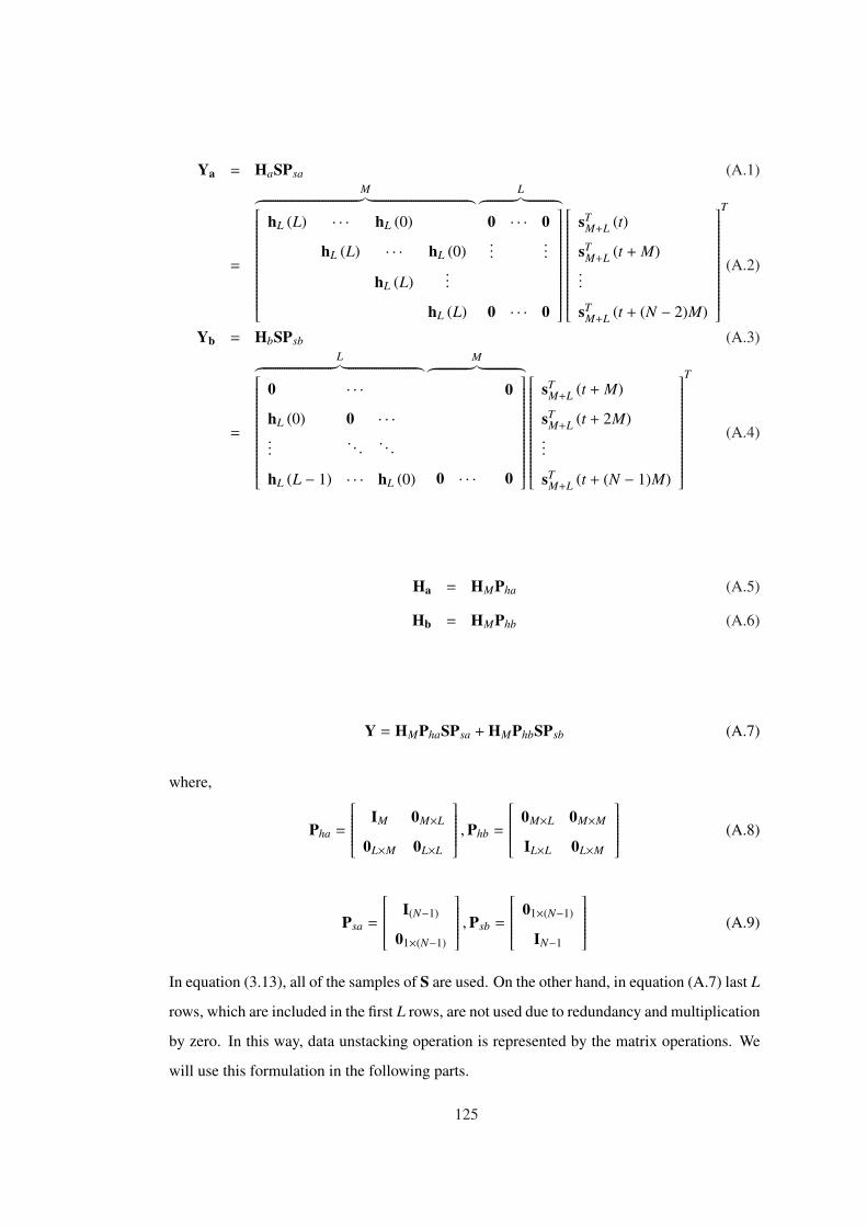
Ya = HaSPsa (A.1)

=

M︷︸︸︷

hL (L) · · · hL (0)

hL (L) · · · hL (0)

hL (L)...

hL (L)

L︷︸︸︷0 · · · 0...

...

0 · · · 0

sTM+L (t)

sTM+L (t + M)...

sTM+L (t + (N − 2)M)

T

(A.2)

Yb = HbSPsb (A.3)

=

L︷︸︸︷

0 · · ·hL (0) 0 · · ·...

. . .. . .

hL (L − 1) · · · hL (0)

M︷︸︸︷0

0 · · · 0

sTM+L (t + M)

sTM+L (t + 2M)...

sTM+L (t + (N − 1)M)

T

(A.4)

Ha = HMPha (A.5)

Hb = HMPhb (A.6)

Y = HMPhaSPsa + HMPhbSPsb (A.7)

where,

Pha =

IM 0M×L

0L×M 0L×L

,Phb =

0M×L 0M×M

IL×L 0L×M

(A.8)

Psa =

I(N−1)

01×(N−1)

,Psb =

01×(N−1)

IN−1

(A.9)

In equation (3.13), all of the samples of S are used. On the other hand, in equation (A.7) last L

rows, which are included in the first L rows, are not used due to redundancy and multiplication

by zero. In this way, data unstacking operation is represented by the matrix operations. We

will use this formulation in the following parts.

125

A.2 Lemma 1

The proof of the lemma is based on Theorem-1 defined in [3]. According to this theorem

smoothing error matrix, El is given by equation A.10 for different channel orders l, when the

true channel order is L.

El =

0 , l < L

Hl(h)

st+l−L|Zl

st|Zl

, L ≤ l

(A.10)

where

Hl(h) =

hL(L)...

. . .

hL(0). . . hL(L). . .

...

hL(0)

︸︷︷︸

l−L+1 columns

(A.11)

When the channel order is known, i.e., l = L, the dimension of column space of El is one and

spanned by the channel vector hL. Therefore, the eigenvector corresponding the maximum

eigenvalue of El can be taken as the solution for channel estimation.

In the case of overestimated channel order, i.e., l = L + m and m > 0, the dimension of the

columns space of El is m + 1 and spanned by the columns of Hl(h).

C {El} = C{Hl(h)} (A.12)

Since the channel order is not known, the overestimated channel order is treated as the true

channel order and the solution used in the case of known channel order is considered. In other

words, the eigenvector corresponding the maximum eigenvalue of El is taken as the solution

when l > L. Let us the channel estimate be hl as a result of this solution. hl is in the range

space of El, which is spanned by the columns of Hl(h).

126

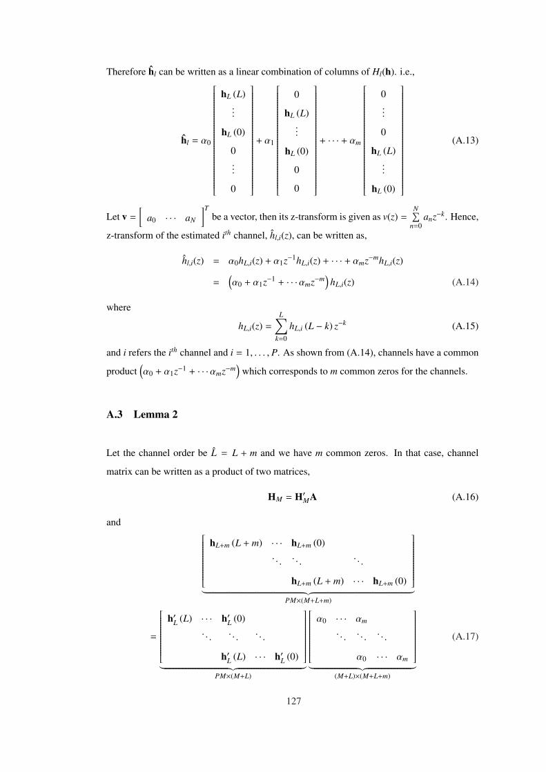
Therefore hl can be written as a linear combination of columns of Hl(h). i.e.,

hl = α0

hL (L)...

hL (0)

0...

0

+ α1

0

hL (L)...

hL (0)

0

0

+ · · · + αm

0...

0

hL (L)...

hL (0)

(A.13)

Let v =

[a0 · · · aN

]Tbe a vector, then its z-transform is given as v(z) =

N∑n=0

anz−k. Hence,

z-transform of the estimated ith channel, hl,i(z), can be written as,

hl,i(z) = α0hL,i(z) + α1z−1hL,i(z) + · · · + αmz−mhL,i(z)

=(α0 + α1z−1 + · · ·αmz−m

)hL,i(z) (A.14)

where

hL,i(z) =

L∑

k=0

hL,i (L − k) z−k (A.15)

and i refers the ith channel and i = 1, . . . , P. As shown from (A.14), channels have a common

product(α0 + α1z−1 + · · ·αmz−m

)which corresponds to m common zeros for the channels.

A.3 Lemma 2

Let the channel order be L = L + m and we have m common zeros. In that case, channel

matrix can be written as a product of two matrices,

HM = H′MA (A.16)

and

hL+m (L + m) · · · hL+m (0). . .

. . .. . .

hL+m (L + m) · · · hL+m (0)

︸︷︷︸

PM×(M+L+m)

=

h′L (L) · · · h′L (0). . .

. . .. . .

h′L (L) · · · h′L (0)

︸︷︷︸

PM×(M+L)

α0 · · · αm

. . .. . .

. . .

α0 · · · αm

︸︷︷︸

(M+L)×(M+L+m)

(A.17)

127

where, the roots of the polynomial, whose coefficients are given as αk, are the common zeros.

Using the property of the rank of the matrix product, following inequality can be written,

rank (HMA) ≤ min {rank (HM) , rank (A)} (A.18)

Rank of the matrices are

rank (HM) ≤ M + L (A.19)

rank (A) ≤ M + L (A.20)

As a result of inequality (A.18), the rank of HM is equal or less than M + L, which is smaller

than the number of columns of HM. Therefore the channel matrix, HM , is not full column

rank.

A.4 Lemma-3

In Lemma-1, it is shown that, hl can be written as a linear combination of the columns of

Hl(h). Consider that l = L + 1 and define h1 and h2 as the two columns of Hl(h). Then,

hl = ah1 + bh2 (A.21)

where,

h1 =

hL(L)...

hL(0)

0

, h2 =

0

hL(L)...

hL(0)

(A.22)

and a + bz−1 is the transfer function of common zero. If |a| = |b|, then the common zero is

located on the unit circle.

Let the eigenvectors spanning the columns of Hl(h) or El be e1 and e2 with corresponding

eigenvalues λ1 > λ2. Since h1 and h2 are also in the column space of El, they can be written

as a linear combination of e1 and e2 as follows.

h1 = α1e1 + β1e2

h2 = α2e1 + β2e2

(A.23)

128

In LSS algorithm, channel estimate for the channel order, l is given as the eigenvector corre-

sponding the maximum eigenvalue of ElEHl . Therefore, h,l = e1 if the scale factor is assumed

to be one. If the equation (A.21) is multiplied by eH1 from left, it is obtained that a = α1.

In the same manner, if the equation (A.21) is multiplied by eH2 from left, it is obtained that

b = α1. Hence if we show that |α1| = |α2|, the proof will be completed.

Hl(h)Hl(h)H can be written in terms of eigenvectors e1 and e2 as follows.

Hl(h)Hl(h)H = λ1e1eH1 + λ2e2eH

2 (A.24)

Another equation can be obtained from the structure of h1 and h2.

‖h1‖ = ‖h2‖ (A.25)

hH1 h1 = hH

2 h2 (A.26)

Replacing (A.23) in (A.26),

|α1|2 + |β1|2 = |α2|2 + |β2|2 (A.27)

Multiplying (A.24) from left by eH1 and from right by e1,

|α1|2 + |α2|2 = λ1 (A.28)


|β1|2 + |β2|2 = λ2 (A.29)


α1

α2= −β1

β2= c (A.30)

As a summary, we have the following equations to be used for the proof of lemma. We want

to show that |α1| = |α2|.

|α1|2 + |β1|2 = |α2|2 + |β2|2 (A.31)

|α1|2 + |α2|2 = λ1 (A.32)

|β1|2 + |β2|2 = λ2 (A.33)α1

α2= −β1

β2= c (A.34)

129

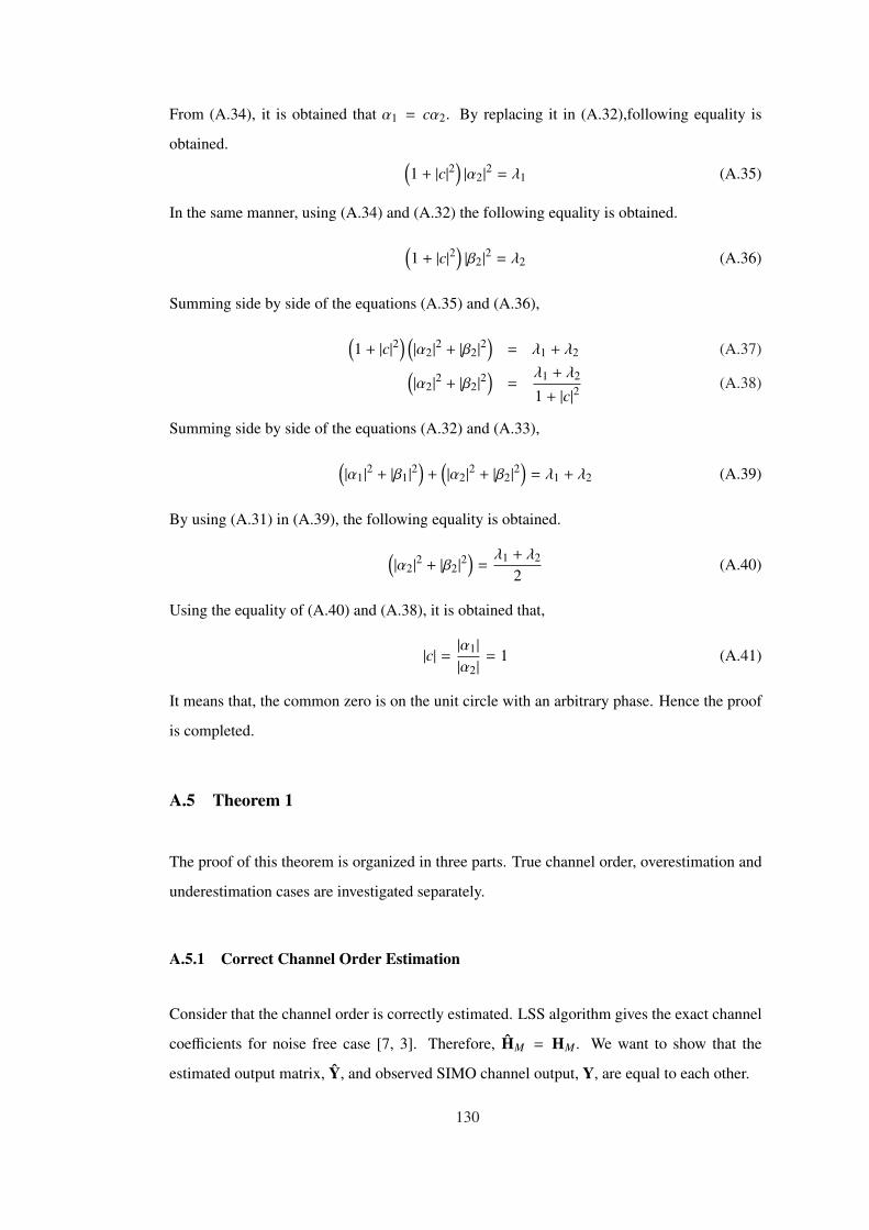
From (A.34), it is obtained that α1 = cα2. By replacing it in (A.32),following equality is

obtained.(1 + |c|2

)|α2|2 = λ1 (A.35)

In the same manner, using (A.34) and (A.32) the following equality is obtained.

(1 + |c|2

)|β2|2 = λ2 (A.36)

Summing side by side of the equations (A.35) and (A.36),

(1 + |c|2

) (|α2|2 + |β2|2

)= λ1 + λ2 (A.37)

(|α2|2 + |β2|2

)=

λ1 + λ2

1 + |c|2 (A.38)

Summing side by side of the equations (A.32) and (A.33),

(|α1|2 + |β1|2

)+

(|α2|2 + |β2|2

)= λ1 + λ2 (A.39)

By using (A.31) in (A.39), the following equality is obtained.

(|α2|2 + |β2|2

)=λ1 + λ2

2(A.40)

Using the equality of (A.40) and (A.38), it is obtained that,

|c| = |α1||α2| = 1 (A.41)

It means that, the common zero is on the unit circle with an arbitrary phase. Hence the proof

is completed.

A.5 Theorem 1

The proof of this theorem is organized in three parts. True channel order, overestimation and

underestimation cases are investigated separately.

A.5.1 Correct Channel Order Estimation

Consider that the channel order is correctly estimated. LSS algorithm gives the exact channel

coefficients for noise free case [7, 3]. Therefore, HM = HM . We want to show that the

estimated output matrix, Y, and observed SIMO channel output, Y, are equal to each other.

130

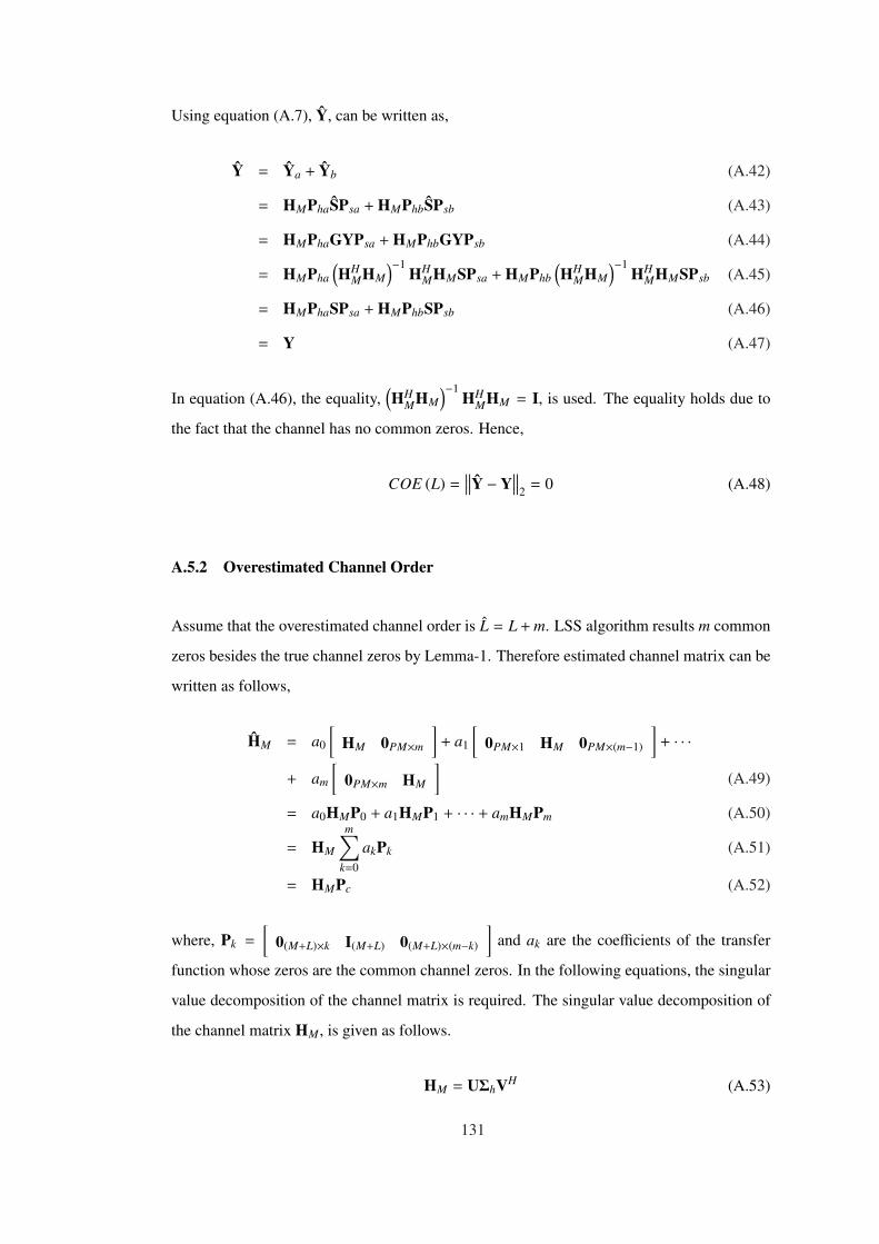
Using equation (A.7), Y, can be written as,

Y = Ya + Yb (A.42)

= HMPhaSPsa + HMPhbSPsb (A.43)

= HMPhaGYPsa + HMPhbGYPsb (A.44)

= HMPha(HH

MHM)−1

HHMHMSPsa + HMPhb

(HH

MHM)−1

HHMHMSPsb (A.45)

= HMPhaSPsa + HMPhbSPsb (A.46)

= Y (A.47)

In equation (A.46), the equality,(HH

MHM)−1

HHMHM = I, is used. The equality holds due to

the fact that the channel has no common zeros. Hence,

COE (L) =∥∥∥Y − Y

∥∥∥2 = 0 (A.48)

A.5.2 Overestimated Channel Order

Assume that the overestimated channel order is L = L + m. LSS algorithm results m common

zeros besides the true channel zeros by Lemma-1. Therefore estimated channel matrix can be

written as follows,

HM = a0

[HM 0PM×m

]+ a1

[0PM×1 HM 0PM×(m−1)

]+ · · ·

+ am

[0PM×m HM

](A.49)

= a0HMP0 + a1HMP1 + · · · + amHMPm (A.50)

= HM

m∑

k=0

akPk (A.51)

= HMPc (A.52)

where, Pk =

[0(M+L)×k I(M+L) 0(M+L)×(m−k)

]and ak are the coefficients of the transfer

function whose zeros are the common channel zeros. In the following equations, the singular

value decomposition of the channel matrix is required. The singular value decomposition of

the channel matrix HM, is given as follows.

HM = UΣhVH (A.53)

131

Since the channel matrix is full column rank due to the assumption A1, Σh has the following

form,

Σh =

λ1. . .

λM+L

0 · · · 0

=

Λh

0

(A.54)

Estimated output signal, Y, is composed of Ya and Yb, which are defined in equations (A.1)

and (A.3) respectively. It will be easier to determine Ya and Yb separately and then compute

Y = Ya + Yb.

Ya = HMPhaSPsa (A.55)

= HMPhaGYPsa (A.56)

= HMPha(HH

MHM)†

HHMHMSPsa (A.57)

= HMPcPha(PH

c HHMHMPc

)†PH

c HHMHMSPsa (A.58)

= HMPcPha

(PH

c VΣHh UHUΣhVHPc

)†PH

c VΣHh UHUΣhVHSPsa (A.59)

= HMPcPha

(PH

c VΛ2hVHPc

)†PH

c VΣHh ΣhVHSPsa (A.60)

= HMPcPha(Pc

)† (VΛ2hVH

)−1 (PH

c

)†PH

c VΛ2hVHSPsa (A.61)

= HMPcPha(Pc

)†VΛ−2h VHVΛ2

hVHSPsa (A.62)

= HMPcPha(Pc

)†VΛ−2h Λ2

hVHSPsa (A.63)

= HMPcPha(Pc

)† SPsa (A.64)

where Pc =m∑

k=0akPk and G =

(HH

MHM)†

HHM. Pha, Phb; and Psa and Psb are the matrices in

equations (A.8) and (A.9) for the channel order, L + m, respectively. In equation (A.61), the

following property of Moore-Penrose pseudoinverse is used. If A is full column rank and B is

full row rank then; (AB)† = B†A†. Note that Pc is a full row rank and VΛ2hVH is a full rank

matrix.

In the same manner Yb can be found as,

Yb = HMPcPhb(Pc

)† SPsb (A.65)

Then the output Y is written as,

Y = Ya + Yb = HMPcPha(Pc

)† SPsa + HMPcPhb(Pc

)† SPsb (A.66)

132

In order to compare Y and Y, equation (A.66) should be modified. In this respect, PcPha(Pc

)†

and PcPhb(Pc

)† in equation (A.66) are written as follows,

PcPha (Pc)† =

IM×M 0M×(L+m)

AL×M BL×(L+m)

(A.67)

PcPhb (Pc)† =

0M×(M+L+m)

C(L+m)×(M+L+m)

(A.68)

where A, B, and C are non-zero and non-identity matrices and m > 0. Furthermore Y, HM,

and S matrices are written in the following form,

S =

Sa

Sb

, Ya =

Ya1

Ya2

, HM =

Hx 0

Hy Hz

(A.69)

where Sa, Sb, Ya1, Ya2, Hx, Hy and Hz are M×N, (L + m)×N, P (M − L − m)×N, P (L + m)×N, P (M − L − m) × M, P (L + m) × M, P (L + m) × L matrices respectively. Output matrix,

Ya, can be written with these matrix formations as follows,

Ya = HMPhaSPsa (A.70)

=

Hx 0

Hy Hz

IM×M 0M×L

0L×M 0L×L

SPsa =

Hx 0

Hy Hz

Sa

0

Psa (A.71)

=

HxSaPsa

HySaPsa

(A.72)

In the same manner, Ya can be written as,

Ya = HM[PcPha (Pc)†

]SPsa (A.73)

=

Hx 0

Hy Hz

IM×M 0M×L

AL×M BL×L

SPsa =

Hx 0

Hy Hz

Sa

ASa + BSb

Psa (A.74)

=

HxSaPsa

HySaPsa + Hz (ASa + BSb) Psa

(A.75)

From equations (A.72) and (A.75), it is seen that, Ya1 = Ya1 and Ya2 , Ya2.

The similar equations can be written for Yb and Yb. Now rearrange the matrices in the fol-

lowing way to write Yb,

S =

Sb

Sc

, Yb =

Yb1

Yb2

(A.76)

133

where Sb, Sc, Yb1, Yb2 are (L + m) × N, M × N, P (M − L − m) × N, P (L + m) × N matrices

respectively. Using these matrix formations, output matrix Yb can be written as,

Yb = HMPhbSPsb (A.77)

=

Hx 0

Hy Hz

0M×L 0M×M

IL×L 0L×M

SPsb =

Hx 0

Hy Hz

0

Sb

Psb (A.78)

=

0(M−L−m)×N

HzSbPsb

(A.79)

In the same manner, Yb can be written as,

Yb = HM[PcPhb (Pc)†

]SPsb =

Hx 0

Hy Hz

0

C

SPsb =

0(M−L−m)×N

HzCSbPsb

(A.80)

From equations (A.79) and (A.80) it is seen that, Yb1 = Yb1 and Yb2 , Yb2.

The result is that, when m > 0, first M− L−m rows of Y are identical with the channel output

Y. When M ≥ L + m, Y samples will be erroneous and the cost function is greater than zero,

i.e.,

COE (L + m) =∥∥∥Y − Y

∥∥∥2 (A.81)

= ‖Hz (ASa + BSb) Psa + Hz (C − I) SbPsb‖2 > 0 (A.82)

A.5.3 Underestimated Channel Order

When the channel order is underestimated, channel coefficients can not be estimated because

of the reason that the smoothing error matrix, El = 0 [3, pg.234, eq.25]. Therefore channel

coefficients are not correctly estimated and there is always a nonzero error. This leads to

nonzero error in channel equalization and∥∥∥Y − Y

∥∥∥2 > 0.

A.6 Theorem-2

For the proof of the theorem, correctly estimated channel order, overestimated channel order

and under estimated channel order cases are studied separately to show that the cost function

defined in (3.24) is zero only when the channel order is correctly estimated in noise free case.

134

A.6.1 Correct Channel Order Estimation

Consider that the channel order is correctly estimated, i.e. L = L. LSS algorithm finds the

true channel coefficients in the noise free case, when the true channel order is given [7, 3].

Therefore, H(L)M = H(L)

M . We want to show that the cost function defined through equation

(3.24) is equal to zero when L = L, i.e. ECMR(L) = 0.

According to Lemma-1, when the channel order is overestimated by one, one common zero

is added to true channel transfer function. In this case, channel matrix H(L+1)M can be written

as the product of the true channel matrix, H(L)M , and the matrix, H(1)

c .

H(L+1)M = H(L)

M H(1)c (A.83)

Since the channel coefficients are estimated exactly for the true channel order, channel matrix,

HLM, is full column rank under assumption that there is no common zeros between SIMO

channels. Therefore,(H(L)

M

)†H(L)

M = I (A.84)

The matrix, A , can be written as follow.

A = F �((

H(L)M

)†H(L+1)

M

)(A.85)

= F �((

H(L)M

)†H(L)

M H(1)c

)(A.86)

= F �(H(1)

c

)(A.87)

= H(1)c (A.88)

Replacing, A, in equation (3.24), the cost function is obtained as follows,

ECMR (L) =∥∥∥∥H(L+1)

M −H(L)M H(1)

c

∥∥∥∥2/∥∥∥∥H(L+1)

M

∥∥∥∥2

(A.89)

=∥∥∥∥H(L+1)

M −H(L+1)M

∥∥∥∥2/∥∥∥∥H(L+1)

M

∥∥∥∥2

(A.90)

= 0

A.6.2 Overestimated Channel Order

Consider that the channel order is overestimated, i.e., L = L + m and m > 0. As noted before,

the function of F is to extract the Toeplitz form from the matrix Bm. If Bm has Toeplitz matrix

135

with first row equal to [bm(0) bm(1) 0 · · · 0] and first column equal to [bm(0) 0 · · · 0]T , then

Am = Bm. If this is the case,

H(L+m)M Am = H(L+m)

M Bm (A.91)

= H(L+m)M

(H(L+m)

M

)†H(L+m+1)

M (A.92)

= H(L)M H(m)

c

(H(L)

M H(m)c

)†H(L+m+1)

M (A.93)

= H(L)M H(m)

c

(H(m)

c

)† (H(L)

M

)†H(L+m+1)

M (A.94)

= H(L)M

(H(L)

M

)†H(L+m+1)

M (A.95)

= H(L)M

(H(L)

M

)†H(L)

M H(m+1)c (A.96)

= H(L)M H(m+1)

c (A.97)

= H(L+m+1)M (A.98)

and ECMR(L) in (3.24) becomes zero. H(m)c and H(L)

M are full row rank and full column rank

matrices respectively. Therefore,(H(L)

M H(m)c

)†=

(H(m)

c

)† (H(L)

M

)†in (A.93) as result of prop-

erties of Moore-Penrose pseoudeinverse. In the same manner, H(m)c

(H(m)

c

)†= I in equation

(A.94) and(H(L)

M

)†H(L)

M = I in equation (A.96). ECMR(L) is different than zero as long as Am

is not equal to Bm or Bm is not a Toeplitz matrix with two coefficients. In this proof, it is

shown that B can not become a Toeplitz matrix for m > 0.

The proof will be by contradiction. So let us first assume that B is Toeplitz matrix with the

formation described in the previous paragraph. In (A.98) it is also shown that H(L+m+1)M =

H(L+m)M Bm. Replacing H(L+m+1)

M in (3.26),

Bm =(H(L+m)

M

)†H(L+m+1)

M (A.99)

=(H(L+m)

M

)†H(L+m)

M Bm (A.100)

= PBm (A.101)

where P =(H(L+m)

M

)†H(L+m)

M , I, because H(L+m)M is not full column rank as a result of Lemma-

1 and Lemma-2. When Bm is a Toeplitz matrix, PBm can not be a Toeplitz matrix with same

formation, i.e. PBm , B. Equality only holds when P = I, which is not the case when m > 0,

because channel matrix is not full column rank. Hence it contradicts with the assumption

about Bm, which states that Bm can not be a Toeplitz matrix with two coefficients. Therefore

ECMR(L + m) > 0 for m > 0.

136

A.6.3 Underestimated Channel Order

When the channel order is underestimated, the channel coefficients are not correctly estimated

[3] and this leads to nonzero cost function for underestimated channel orders.

137

CURRICULUM VITAE

PERSONAL INFORMATION

Surname, Name: Karakutuk, SerkanNationality: Turkish (TC)Date and Place of Birth: 1978 , AnkaraPhone: +90 542 560 71 61email: [email protected]

EDUCATION

Degree Institution Year of GraduationMS METU, Electrical and Electronics Engineering, Ankara 2003BS Gazi University, Electrical and Electronics Engineer-

ing, Ankara2000

High School Arı Science High School, Ankara 1995

WORK EXPERIENCE

Year Place Enrollment2005- MIKES System Engineer2003-2005 Education and Research Foundation of METU Prof. Dr.

Mustafa N. PARLARRD Engineer

2000-2003 Baskent University Research Assistant

FOREIGN LANGUAGES

Advanced English

PUBLICATIONS

1. S. Karakutuk, T. E. Tuncer, Effects of Modulation Type on Blind SIMO CommunicationsSystems, Signal Processing and Communication Applications, 2007. SIU 2007, Vol.15, pp.1 − 4, 11-13 June 2007.2. S. Karakutuk, T. E. Tuncer, Channel output error (COE) for channel order estimation,Signal Processing and Communication Applications, 2009. SIU 2009, pp. 57 − 60, April2009.3. S. Karakutuk, T. E. Tuncer, A new channel order estimation algorithm for FIR SIMOchannels, 17th European Signal Processing Conferece, EUSIPCO-2009, August 2009.

138

blind and semi-blind channel order estimation in simo...

Documents