black economy and demonetisationepu/acegd2018/papers/snehaagrawal.pdf · black economy and...
TRANSCRIPT
Black Economy and Demonetisation∗
Sneha Agrawal †
May, 2018
Abstract
On 8th November 2016, Government of India announced the surprise ‘Demonetisation’of |500 (US $7.70) and |1000 (US $15) bank notes replacing them with new notes. Thegovernment claimed that this action would curtail the shadow economy and crack downthe use of illicit and counterfeit cash to fund illegal activity. The sudden nature of theannouncement and the prolonged cash shortages in the weeks that followed - created sig-nificant disruption throughout the Indian economy. In this paper, we build a theoreticalframework to explain some of the stylised facts of demonetisation in India and characteriseit’s implications on the Stationary monetary equilibrium of the economy. The paper closelyexplains the tradeoff faced by the agents with regards to holding black money and evadingtaxes on one hand and getting heavily penalised if caught by the auditors on the other. Themodel also explains how money laundering naturally emerges when the government compelsagents to reveal their true taxable incomes via demonetisation.
∗Preliminary draft. Thanks to Prof. Ricardo Lagos for his invaluable advice and support. Thanks to AbhishekGaurav for all the discussions, and all the participants at the Macro Student Lunch, NYU for their commentsand suggestions.†New York University
1
1 Introduction
Economies all across the world, have been facing (in varying degrees), the existence of ‘BlackEconomy’/ ‘Shadow Economy’ and taking measures to mitigate the issues it entails - blackmoney, counterfeit currency, terrorism, and tax evasion to name a few. One of the most commonmanifestations of black economy is when individuals underreport their incomes or money holdingsin order to evade taxes. The money that individuals use in transactions and for consumptionbut that is not reported for tax purposes is what we shall define as ‘Black Money’ in this paper.
Historically, many economies have dealt with this issue of black money through different formsof regulations - be it random tax audits, raids by revenue department on rich business firms, hugepenalties for defaulters, or some other non-conventional measures. One such non-conventionalmeasure was taken in India on 8th November 2016 with a sudden/ unexpected announcement of‘Demonetisation’ of it’s 2 highest denomination currency. It meant stripping the |500 (≈ 7.5$)and |1000 (≈ 15$) notes of their status as legal tender and replacing them with newly issued|500 and |2000 notes (on the left and right in Figure 1 respectively).
Figure 1: Old notes and New Notes in India, Demonetisation 2016
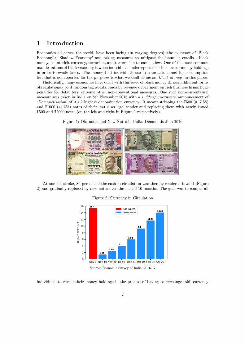
At one fell stroke, 86 percent of the cash in circulation was thereby rendered invalid (Figure2) and gradually replaced by new notes over the next 6-10 months. The goal was to compel all
Figure 2: Currency in Circulation
Source: Economic Survey of India, 2016-17
individuals to reveal their money holdings in the process of having to exchange ‘old’ currency
2
notes for ‘new’ from the government at par value. As a result, all the agents who held blackmoney, had 3 options: (i) Declare their unaccounted wealth and pay taxes at a penalty rate,(ii) Continue to hide it, not converting their old notes and thereby suffering a tax rate of 100%,(iii) or Launder their black money by paying a cost for converting the money into ‘white’ (legalmoney). These notes were to be deposited in the banks by December 30, 2016 after which theywould be rendered valueless in terms of legal tender i.e. the government would not honour themanymore. This goes back to the classic definition of unbacked fiat money - while the papercurrency is not backed by actual physical goods, it is used as a money because it is backed bygovernment/ monetary authority’s promise/ fiat to honour it.
In this paper, we formalise a model to capture all these nuances when demonetisation happensand understand the implications of such a policy on the ‘Black Economy’ and the MonetaryEquilibrium. The model uses a simplified specification of the ‘Lagos and Wright (2005)’ [L]framework with heterogenous agents (in terms of money holdings). It then adds the possibilityof black money in the baseline model. Finally, we incorporate sudden demonetisation into theeconomy with some agents holding black money and see the implications for the MonetaryEquilibrium.
One place where the black economy is predominantly effective in the Indian Economy is theinformal sector - where most of the transactions are made off the books and agents have regulartransactions in cash. We shall try to model the use of money for transactions between buyers andsellers, but potentially not declared for tax returns, as those, which happen in the cash intensiveinformal sector. The other part of the economy would be the more formal one, where agentsproduce and consume in a competitive market and make their inter-temporal money holdingdecisions. They may be required to pay taxes and they get some transfers from the government.
In Section 2, we understand the baseline model with prevalence of black money holders andrandom checks by the government. In Section 3, we expand the model to incorporate a onetime ‘Demonetisation’ policy and understand how the Monetary Equilibrium changes due to thepolicy. Finally, we conclude with some policy implications and assess the success/ failure of thepolicy.
3
2 Baseline Model of Black Money
2.1 Primitives
We consider an infinite horizon discrete time model. Each unit of time consists of 2 sub-periodseach designated to a certain type of good. The first subperiod is for the production and exchangefor the ‘Specialised Goods’ in a ‘Decentralised Market’ (DM) using search and bargaining; whilethe second is for the production and consumption of a ‘General Good’ in a ‘Centralised Market’(CM). Both types of goods are non-storable and perfectly divisible. Specialised goods are het-erogenous and only produced by ‘Specialists/ Sellers’ while general goods are homogeneous andproduced by all the agents. The general good is the numeraire.
There are two categories of agents in the economy depending on their role in the decentralisedmarket - a unit mass of ‘Buyers’ (B) who consume specialised goods and a unit mass of ‘Sellers/Specialists’ (S) who produce these specialised goods. Buyers and Sellers meet each other withprobability α in this market and once they do, seller produces the amount of good the buyerneeds and the buyer pays the cost to the seller using money. Money is the only non-storableperfectly-divisible medium of exchange in this economy. For simplicity, we shall assume that thebuyers have all the bargaining power in this bilateral exchange.
In the centralised market, all the agents are endowed with 1 unit of labor. All agents producethe general good and they can consume it, or sell some of it to take money into the next period.There is perfectly persistent heterogenous productivity among agents i.e. they have differentdisutility from production. For the sellers, there is uniform disutility of 1 from putting ht unitsof labor. On the other hand, buyers are randomly assigned a productivity level at the start oftheir life - with probability πL, they have low productivity i.e. the disutility cost of providing hunits of labor into production of general good is high (h/εL), and with probability πH = 1− πL,they have high productivity i.e. it costs less (h/εH), εH > εL.
Consequently agents maximize the following objective function,
E0
∞∑t=0
βt[u(qbt )− c(qst ) + log ct −
htεt
](1)
where β ∈ (0, 1), qbt and qst are the consumption and production of specialised goods in the firstsubperiod and ct and ht are consumption and hours worked in the second subperiod of time t. εtis the productivity level in the second subperiod ∈ {1, εL, εH} for seller and buyer of each typerespectively. This is how we consider a simplified model from [L] .
We shall assume that u′ > 0, u′′ < 0, c′ > 0, c′′ ≥ 0, u(0) = c(0) = 0 and ∃q, q∗ such thatu(q) = c(q) and u′(q∗) = c′(q∗).
All agents in this economy face an exogenous shock of death with probability δ at the be-ginning of the second subperiod of time t which means that they’ll exit from the economy t+ 1onwards. To ensure a stationary mass of population, a fraction ν of people will be born andexogenously assigned a type {B, εL}, {B, εH} or {S} with probability 0.5πL, 0.5πH , 0.5 respec-tively.
There is a single financial instrument, ‘Fiat Money’. The stock of money at time t is denotedbyMt withM0 ∈ R++. A monetary authority (we might also refer to it as government sometimes)injects or withdraws money via lump sum transfers St in the second subperiod of every periodin order to implement a constant growth of money supply i.e. Mt+1 = µMt with µ > 0. Atthe beginning of life, each agent is therefore endowed with their type - Buyer/ Seller (whichdetermines their labor endowment), perfectly persistent productivity if they are buyer and aportfolio of money.
4
The agents’ type, money holdings and bilateral transactions are common knowledge amongthemselves, but to the government, they are unobservable. The government has a tax-penaltypolicy, (lump sum for now) whereby it imposes a lump sum tax T on more productive agents(who turn out to be the buyers with much higher money holdings i.e. rich agents in the model)and no tax (T = 0) for the low productivity buyers (also the agents with lower money holdings).This tax is required to be paid at the start of the second sub-period in terms of general goods.There are no taxes on Sellers since their type is always known and they are mere facilitators inthis model to support the more interesting side of heterogenous buyers. Since the governmentcannot observe the type of buyers, it imposes the tax based on reported types ε i.e.
T (ε) =
{T if ε = εH
0 otherwise(2)
This is what leads to possible mis-reporting by the agents. In particular, rich/high productivityagents want to misreport themselves as low type in order to evade taxes i.e. they can potentiallyuse money for transaction with sellers and other agents without declaring it for tax purposes. Thisis what leads to ‘Black Money’ in the economy. In order to check this misreporting behavior, thegovernment randomly audits the buyers who report themselves to be low type, with probabilityp. If they are caught under-reporting, it imposes a lump sum penalty in terms of general goodsP(> T) i.e.
P (ε, ε) =
{P if ε = εL 6= ε = εH
0 if ε = εL = ε = εL(3)
In this simple model, the government need not audit the agents who already report to be highproductivity because they are paying taxes honestly anyway. Finally, we shall assume that agentscannot make binding commitments; and trading histories are private in a way that precludes anyborrowing and lending between people. So, all trade - both in the centralised market and thedecentralised markets must be quid pro quo.
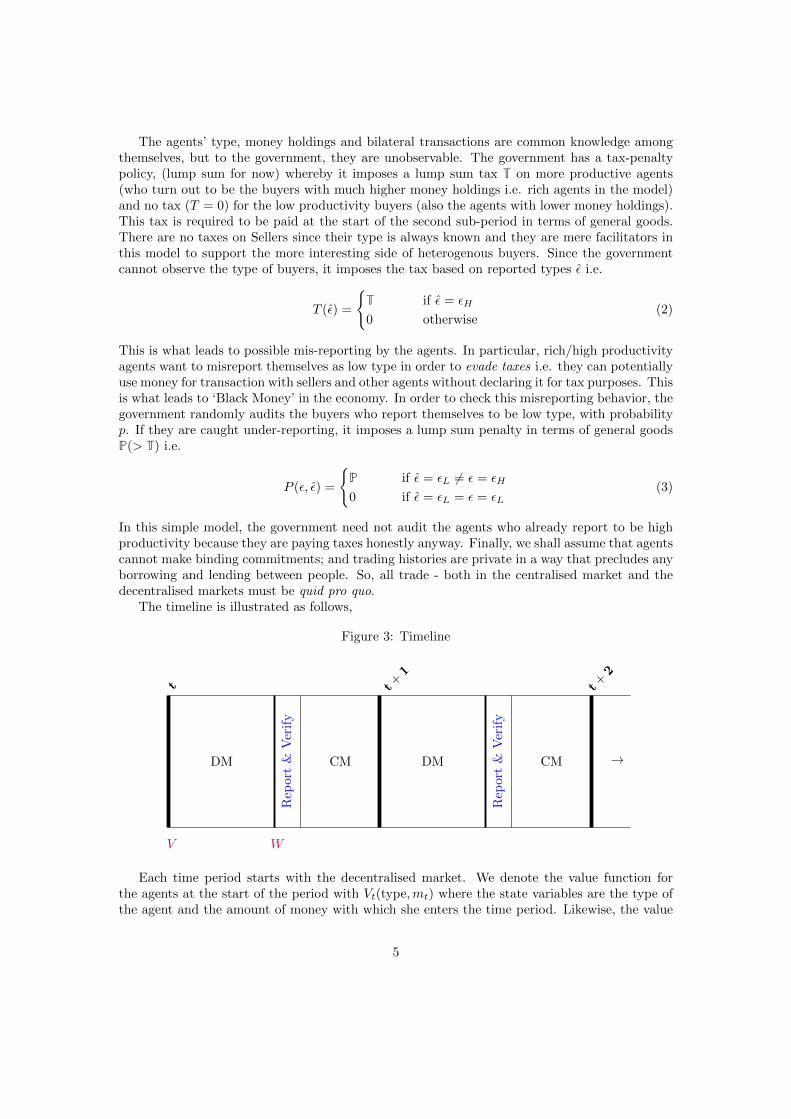
The timeline is illustrated as follows,
Figure 3: Timeline
t
V
DM
W
Rep
ort
&V
erif
y
CM
t +1
Rep
ort
&V
erif
y
DM CM
t +2
→
Each time period starts with the decentralised market. We denote the value function forthe agents at the start of the period with Vt(type,mt) where the state variables are the type ofthe agent and the amount of money with which she enters the time period. Likewise, the value
5
function at the start of the second subperiod is denoted by Wt(type,mt). Conditional on no exit/death shock, the second subperiod starts with the agents reporting their type, the governmentrandomly auditing them, appropriate payment of tax/penalty/nothing, and finally consumptionand saving decision in the centralised market. If the agents face the death shock, they consumewhatever they have in that period and exit the economy.
Let types ∈ {S,L,C,NC} where S denotes the Seller, L are the buyers with Low Productivity,C are the high productivity buyers who either pay the taxes honestly or have been ‘Caught’ inthe past so that their perfectly persistent type is revealed forever, and NC be the high typebuyers who underreport their type and have ‘Not been Caught’ so far. We shall see that thistype space is rich enough to model black money in the economy. We shall denote money holdingsof buyers at time t as mt and that of seller as mt. Let the distribution of money holdings acrossbuyers be F (m) and that for sellers be G(m).
2.2 Value Functions and Optimal Decisions
Given the primitives, we can now solve for the optimal decisions and values for each type ofagent and characterise the Monetary Equilibrium. The details of the derivations are given inthe appendix A.1. Let φt denote the price of money in terms of general goods at time t. Then,the value function at the start of the second subperiod, of each type i of agent who enters withmoney mt denoted by W i
t (mt), is as follows1,
WSt (mt) = −1 + φtm+ φtSt + (1− δ) max
m′
(βV St+1(m′)− φtm′
)(4)
WLt (mt) = log εL − 1 +
φtmt + φtStεL
+ (1− δ) maxm′
[βV Lt+1(m′)− φtm
′
εL
](5)
WCt (mt) = log εH − 1 +
(φtmt − T) + φtStεH
+ (1− δ) maxm′
[βV Ct+1(m′)− φtm
′
εH
](6)
WNCt (mt) = log εH − 1 +
φtmt + φStεH
+ 1ε=εH
[−TεH
+ (1− δ) maxm′
(βV Ct+1(m′)− φm′
εH
)]+
1ε=εL
[p
(−PεH
+ (1− δ) maxm′
[βV Ct+1(m′)− φm′
εH
])+ (1− p)
((1− δ) max
m′
[βV NCt+1 (m′)− φm′
εH
])](7)
The sellers and low type buyers simply come in to the second subperiod and make theiroptimal consumption, labor input, and savings decisions. The high type ‘Caught’ buyers alsohave to pay taxes worth T units of general good each period. The high type ‘Not Caught’ agentsare required to also choose a reporting strategy. If they decide to turn honest from period tonwards, they pay taxes and their value function switches to V Ct+1. If on the other hand theychoose to misreport, they get caught with some probability p, pay a penalty and switch toV Ct+1, else with probability (1− p), they continue to be ‘NC’ type and ‘evade taxes’. These areagents in the economy who shall be rich and potentially holding ‘black money’ for given value ofgovernment audit probability p. Note that the structure of the problem, induces quasi linearityin the value function W w.r.t. m i.e.
W it (mt) =
φtmt
εi+W i
t (0) ∀i ∈ {S,L,C,NC} (8)
which we shall use later when we solve the bargaining problem for the Decentralised market.
1The derivations follow very closely from [L].
6
Having solved for the value functions at the start of second subperiod, we can move backwardsto solve for the value functions V it (mt) at the start of the first subperiod at time t for agent i whoenters the time period with money holdings mt. The buyers and sellers meet each other withprobability α in the DM and enter into Nash Bargaining for exchange of the ‘Specialised Good’.We assume that the buyer has all the bargaining power, and she pays with money d ≤ mt inexchange of the goods qBt she buys. This leads to the following Nash Bargaining problem for thebuyer with money holdings mt, productivity εi who meets a seller with money holdings mt, andhas an outside option of no exchange payoff,
maxqB ,d
ut(qBt (mt, εi, mt)) +W i
t (mt − d(mt, εi, mt))−W it (mt)
subject to − ct(qBt (mt, εi, mt)) +WSt (mt + d(mt, εi, mt))−WS
t (mt) ≥ 0 (9)
The terms of trade for the bargain could in principle depend on buyers type and money holdingsand on the sellers initial money holdings. It turns out that given our assumptions, the buyerexhausts all her money holdings to get as much of the ‘Specialised good’ as she can, and shecompensates the seller enough to break even. The optimal decision is solved in detail in theappendix A.2, and we get the following,
qBt (mt, εi) =
{q∗t (mt, εi) if ct(q
∗t (mt, εi)) ≤ φtmt
{qt|ct(qt(mt, εi)) = φtmt} otherwise(10)
dt(mt, εi) =
ct(q
∗t (mt, εi))
φtif ct(q
∗t (mt, εi)) ≤ φtmt
mt otherwise(11)
This leads to the flow payoff in the Decentralised market for each type of agent, and combiningthat with the continuation values, we get their value function at the start of the first subperiodas follows:
V St (mt) = φtmt +WSt (0) (12)
V Lt (mt) = α
[ut(q
Bt (mt, εL))− ct(q
Bt (mt, εL))
εL
]+φtmt
εL+WL
t (0) (13)
V it (mt) = α
[ut(q
Bt (mt, εH))− ct(q
Bt (mt, εH))
εH
]+φtmt
εH+W i
t (0), i ∈ {C,NC} (14)
Using these value functions, we can go back to the equations in (4)-(7), substitute for theVt+1’s, and get the value of audit probability p, such that the high type not caught agents chooseto misreport their types and hold black money in a stationary monetary equilibrium.
We solve for the threshold value of p using guess and verify. The idea is to start with the guessthat the value of audit probability is such that the High type NC agent chooses to misreporti.e. her value from misreporting is greater than her value from turning honest. Next, under theguess, we can solve for the optimal value of money holdings for each type of agent. Once wehave the solution to all our agents’ optimisation problem under the guess, we can verify thatindeed the probability of audit is such that the optimal decision with subsequent optimal moneyholdings is for the high type agent to misreport her type. This is explained in detail in AppendixA.3 and it leads to the following threshold value of p∗ and reporting strategy for the High typeNC buyers.
7
ε =
{εL if p ≤ T
P ≡ p∗
εH otherwise(15)
Proposition 1. ∃p∗ = TP ∈ (0, 1), such that for all values of p ≤ p∗, rich agents under-report
their money holdings to evade taxes, i.e. ‘Black Money’ exists in the economy.
The proof follows from the above explanation and the derivation of p∗, as derived in theappendix A.3. We assume that the government audits with a probability less than p∗, such thatthe high type agents misreport their type and we have agents holding ‘Black Money’ in thiseconomy. Given all the value functions and the reporting strategy, we can solve for the optimalamount of money holdings for each type of agent, and we get the following stationary real value ofmoney holdings, zi, i ∈ {S,L,C,NC}, for the case when we assume u(q) = log q, and c(q) = cq.We solve for the more general solution to the agents optimisation problem in the appendix A.3.
zS = 0 (16)
zL =βαεL
µ− β(1− α)(17)
zC = zNC =βαεH
µ− β(1− α)(18)
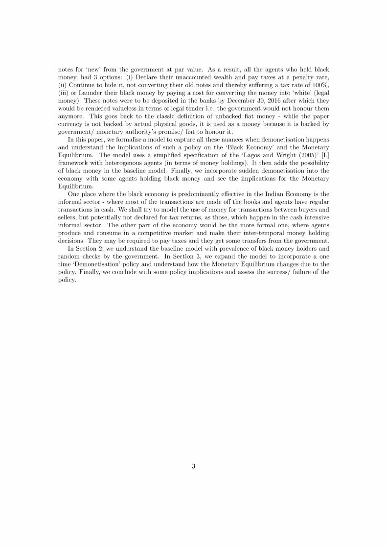
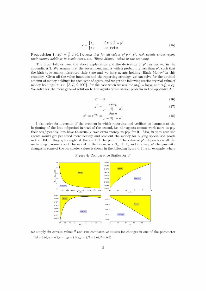
I also solve for a version of the problem in which reporting and verification happens at thebeginning of the first subperiod instead of the second, i.e. the agents cannot work more to paytheir tax/ penalty, but have to actually save extra money to pay for it. Also, in that case theagents would get penalised more heavily and lose out the money for buying specialised goodsin the DM, if they got caught at the start of the period. The value of p∗, depends on all theunderlying parameters of the model in that case, α, ε, β, µ,P,T, and the way p∗ changes withchanges in some of the parameter values is shown in the following figure 4. It is an example, where
Figure 4: Comparative Statics for p∗
we simply fix certain values 2 and run comparative statics for changes in one of the parameter
2β = 0.95, α = 0.5, c = 1, µ = 1.5, εH = 2,T = 0.01,P = 0.02
8

values.Finally, let us look at the laws of motion for the distribution of agents of different types and
impose stationary mass of each type of agent in our stationary monetary equilibrium. Let themeasures be denoted by λ’s. Since, agents of all types die at rate δ and are born at rate ν, weget the following laws of motion for the measure of agents, assuming that 0.5 of the agents areborn as Sellers, 0.5πH as High type Not Caught Buyers and 0.5πL as low type buyers. Also,with probability p, some of the not caught buyers get ‘Caught’. The total measure of buyers andsellers is 1 each respectively.
λS = 0.5ν − δλStλL = 0.5πLν − δλLt
λNC = 0.5πHν − (δ + p)λNC
λC = pλNC − δλCλS = 1, λL + λC + λNC = 1
(19)
Together, we get
λS = 1, λL = πL, λNC =δ
δ + pπH , λC =
p
δ + pπH such that λi = 0,∀i (20)
Also, 0.5ν = δ, so for a given birth/death rate, all the variables are pinned down.
2.3 Stationary Monetary Equilibrium
Given the above model framework, we can now define the Stationary Monetary Equilibrium inthis economy as follows:
Definition 1. Stationary Monetary Equilibrium is the set of perfectly persistent typesof agents i ∈ {S,L,C,NC}, their stationary real money holdings zi, price of money φt > 0,consumption, labor, savings, terms of trade, and reporting choices of the agents; government’smonitoring strategy p, and transfers St, such that :- ∃p∗, and ∀p ≤ p∗, high type agents evadetaxes, all the agents satisfy their value functions (4)-(7) and (12)-(14), terms of trade in DM areas in (10)-(11), all agents choose optimal consumption cit
∗= εi, labor input h∗t , and real money
holdings zi as in (16)-(18), distribution of agents satisfy (19), money market clears as follows,
φt (λLmL + λNCmNC + λCmC) = φtMt = ¯φM (21)
and Government budget equation holds every period, i.e.
φtSt = λCT + λNCpP + φt(Mt+1 −Mt) (22)
This completes our baseline Model with Black Economy, and tax evasion. Next, we wantto consider a ‘surprise announcement’ of Demonetisation at time τ , to an otherwise stationaryequilibrium of this baseline economy, and analyse the best responses of the agents as well theimplications on the monetary equilibrium due to such one time shock.
9

3 Model with Demonetisation
Suppose that at time period τ , the government makes a ‘Sudden Announcement’ that, they aredemonetising all the existing money (which we shall now refer to as ‘Old Money’) and the onlylegal tender from time period τ + 1 onwards, will be the new notes printed by the bank (whichwe shall refer to as ‘New Money’). Also, the agents are given an exchange window at the end ofperiod τ , where they can go and exchange the old notes for new notes, one for one in value. Thisis what we shall refer to as the transition period. From next period, τ + 1, ‘Old Money’ will notlonger be considered legal tender or honoured by the government.
This is like the time period from the announcement of policy in India (Nov 8, 2016), to Dec31, 2018, which was the last day the agents could go to the exchange window and governmentshall convert their old money deposits for new money. Thus, from time period τ , onwards wehave both ‘Old Money’ (denoted by MO) and, ‘New Money’ (denoted by MN ), and hence pricesfor each type of φOτ , and φNτ respectively.
In this model, for what we solve below, we shall assume that, going forward new money ismore valuable in terms of the amount of goods it can buy as compared to old money.
Assumption. φNt+i > φOτ+i ∀i ≥ 1
The timeline with this policy modifies as follows. We basically have the same structure asbefore, but now there is an additional decision to be made at the end of period τ , about howmuch of their old money agents want to exchange for new money at the end of the period. Weshall assume that the agents can only exchange upto their own holdings of old money, i.e. we donot allow for laundering option in this simplified version. Hence, the tradeoff for the agents inthis case is simple, they exchange less valuable old money for more valuable new money, and ifthey try to exchange more money than what their reported type entails, they could get caughtin the process, heavily penalised and their type gets revealed forever.
Figure 5: Timeline with Demonetisation
t Old Money
DM
Rep
ort
&V
erif
y
CM
τ
V
Rep
ort
&V
erif
y
Old + New Money
W
DM CM
τ+
1
Exch
ange
U
→New Money/Old Money/
Both ?
The agents’ problems now comprises of their decisions in the DM and CM, reporting strategy,and also ‘exchange’ strategy. Let V iτ (mO
τ ,mNτ ) and W i
τ (mOτ ,m
Nτ ), be the value functions at the
start of the first and second subperiod respectively, same as before except that both old and newmoney holdings enter their state variable. Further, let us consider value function U iτ (mO
τ ,mNτ )
at the start of the exchange window where the agents chooses how much to exchange, x ≤ mOτ
from her old money holdings. Let the government monitor them based on their reported type
and the amount of money exchanged with probability πi(x), increasing in x (π′(x) > 0). Uponmonitoring the government learns the true type of the agent imposes a fine f i, if the agent
10
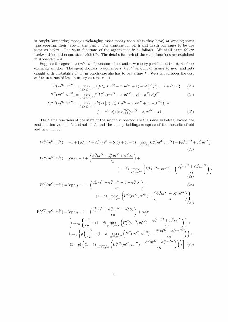
is caught laundering money (exchanging more money than what they have) or evading taxes(misreporting their type in the past). The timeline for birth and death continues to be thesame as before. The value functions of the agents modify as follows. We shall again followbackward induction and start with U ’s. The details for each of the value functions are explainedin Appendix A.4.
Suppose the agent has (m′O,m′N ) amount of old and new money portfolio at the start of theexchange window. The agent chooses to exchange x ≤ m′O amount of money to new, and gets
caught with probability πi(x) in which case she has to pay a fine f i. We shall consider the costof fine in terms of loss in utility at time τ + 1.
U iτ (m′O,m′N ) = max0≤x≤m′O
β[V iτ+1(m′O − x,m′N + x)− πi(x)f i
], i ∈ {S,L} (23)
UCτ (m′O,m′N ) = max0≤x≤m′O
β[V Cτ+1(m′O − x,m′N + x)− πH(x)fC
](24)
UNCτ (m′O,m′N ) = max0≤x≤m′O
πL(x)[β(V Cτ+1(m′O − x,m′N + x)− fNC)
]+
(1− πL(x))[βV NCτ+1 (m′O − x,m′N + x)
](25)
The Value functions at the start of the second subperiod are the same as before, except thecontinuation value is U instead of V , and the money holdings comprise of the portfolio of oldand new money.
WSτ (mO,mN ) = −1 +
(φOτ m
O + φNτ (mN + Sτ ))
+ (1− δ) maxm′O,m′N
USτ (m′O,m′N )−(φOτ m
′O + φNτ m′N)
(26)
WLτ (mO,mN ) = log εL − 1 +
(φOτ m
O + φNτ mN + φNτ Sτ
εL
)+
(1− δ) maxm′O,m′N
{ULτ (m′O,m′N )−
(φOτ m
′O + φNτ m′N
εL
)}(27)
WCτ (mO,mN ) = log εH − 1 +
(φOτ m
O + φNτ mN − T + φNτ SτεH
)+ (28)
(1− δ) maxm′O,m′N
{UCτ (m′O,m′N )−
(φOτ m
′O + φNτ m′N
εH
)}(29)
WNCτ (mO,mN ) = log εH − 1 +
(φOτ m
O + φNτ mN + φNτ Sτ
εH
)+ max
ε[1ε=εH
{−TεH
+ (1− δ) maxm′O,m′N
(UCτ (m′O,m′N )− φOτ m
′O + φNτ m′N
εH
)}+
1ε=εL
{p
(−PεH
+ (1− δ) maxm′O,m′N
(UCτ (m′O,m′N )− φOτ m
′O + φNτ m′N
εH
))+
(1− p)(
(1− δ) maxm′O,m′N
(UNCτ (m′O,m′N )− φOτ m
′O + φNτ m′N
εH
))}](30)
11

For the start of the first subperiod, agents’ value functions are,
V Sτ (mO,mN ) = WSτ (mO,mN ) (31)
V Lτ+1(m′O,m′N ) = αΓLτ+1(m′O,m′N ) +WLτ+1(m′O,m′N ) (32)
V Cτ+1(m′O,m′N ) = αΓHτ+1(m′O,m′N ) +WCτ+1(m′O,m′N ) (33)
V NCτ+1 (m′O,m′N ) = αΓHτ+1(m′O,m′N ) +WNCτ+1(m′O,m′N ) (34)
We solve this model with the above value functions for the optimal amount of money exchangeand savings decisions of each type of agents. Conditional on the amount of old money saved, theagents choose the amount of exchange based on the following tradeoff - higher exchange leads togreater value for money and helps with the gains from more trade in the subsequent Decentralisedmarket, but higher exchange also entails greater probability of getting audited in which case theymight have to pay a fine in case they were holding any amount of black money. We find that fora given audit strategy of the government in the exchange window of the transition period, theagents have a threshold exchange strategy, and the threshold varies depending on agents’ typeand their differential fines. In particular, we get the following optimal Exchange with different,xi, each of them derived in detail in the appendix A.4,
x∗i (m′O,m′N ) = max
{0,min{xi(m′O,m′N ),m′O}
}(35)
where m′O, is the amount of old money the agent has at the start of the Exchange window.We then substitute this optimal exchange strategy into the second period value function andsolve for the optimal money holding decisions (for both old and new notes) for each type ofagent, and consider all the possible exchanges of old money to new for different ranges over theparameter space. The first order conditions are also given in details in the appendix A.4, but theyessentially involve the key tradeoff from savings - the gains from trade in the next decentralisedmarket (same as in the baseline model), the costs of inflation both for a given form of moneyand their relative inflations for old-new money portfolio composition decision, the implication interms of how much of the old money shall be subsequently exchanged and the loss from gettingaudited or having to pay any fines. We consider all the possible sub cases for optimal savings ofold, new notes and optimal exchange. The derivations are given in appendix A.5 for each type ofagents. The final partial equilibrium from the optimisation can be summarised in the followingfigure 6.
In an economy with no demonetisation and 2 possible forms of money, we know that thechoice of money holdings is determined by the relative inflation in the 2 forms, i.e. µNτ ≶ µOτ
3 inour model. This is indicated using the 45◦ line in the figure. The second dimension of decisionmaking for the agents in our model is the tradeoff between getting caught or not, captured bythe threshold strategy x∗i . This decision crucially depends on the probability of monitoring inthe exchange and the threat of fine to be paid when the agents exchange black money. In thefigure, the vertical red line capture this tradeoff, to the left of the line the agent chooses to notexchange any money and too the right, they choose the optimal amount of exchange dependingon their portfolio of old and new money they come into the exchange period with. Finally, themost interesting tradeoff happens to the right of this vertical line and in the case when the oldnotes have higher inflation than the new notes i.e. agents would prefer to hold new money if theywere in the baseline economy. However, with demonetisation and exchange, the tradeoff also getsaffected by the fact that the less valuable old money could be exchanged for more valuable newmoney in the transition period albeit with monitoring. This tilts the tradeoff between old and
3µiτ =φiτφiτ+1
12

Figure 6: Best responses of Type i buyer in Partial equilibrium
µOτ0
µNτ
βεiπifi
∆φτ+1
m′O > xi = 0
m′N = 0
Only OldMoney,No Ex-change
0 < m′O ≤ xim′N = 0
All Old Moneyexchanged to New
m′O = 0,m′N > 0
Only New Money,No Old Moneyto Exchange
Note: The axis of the figures are the inflation in each type of money
new money in favour of old money, which is then exchanged for new money when the fine andprobability of getting caught at the exchange window is sufficiently low. The idea is that theagents can have cheaper old money converted into more valuable new money tomorrow with notmuch risk of getting audited.
The tradeoffs are similar for each type of buyer, but what varies is their costs from gettingcaught in the audit and the amount of money holdings they want to save for the next period.Consequently under the assumption that the agents are punished progressively more from lowtype to the honest high type to the dishonest high type, we get the following partial equilibriumresponses for a given inflation in old and new money and given government regulations.
Assumption. πLfL ≤ πHfC ≤ πLξNC
Thus, the above analysis gives us a complete partial equilibrium of money holdings and ex-change best responses to a given set or prices, and model framework (i.e. government regulations,parameters of the model, money growth etc.)
13

Figure 7: Complete Partial Equilibrium
µOτ0
µNτL
βεLπLfL
∆φτ+1
C
βεHπHfC
∆φτ+1
NC
βεHπLξNC
∆φτ+1
All agents:
Old Money,
No Exchange
Poor:Old → New,
Rich:
Old money,
No exchange
Low, C:Old → New
NC:
Still only
Old money,
No exchange
All types:O → N,
Full exchange
All agents:
Only New Money
Poor: O → N
Full Exchange
Rich:
Only m′N
L, C: O → N
Full Exchange
NC: Only m′N
We interchangeably call the low type buyers as poor agents, and the high type buyers as the rich agents.
4 Monetary Equilibrium
Since, we have already solved and analysed the best responses of each type of agents, we need tonext characterise the general equilibrium in this model, i.e. we need to make sure that the moneymarket clears for both old and new notes and the price for each type of money is determined bytheir relative supply and demand in equilibrium. In particular, we look at each of the sub cases inthe figure and consider the market clearing conditions for old and new money to get equilibriuminflation of each type of money and their exchange rates. So far, we have a preliminary analysisof the kind of equilibrium that emerge. Recall that, we have not allowed for private bilateralmonetary agreements among agents, i.e. we have not allowed for laundering by construction.But since each of the agent faced a different tradeoff in the exchange window, there might beincentives to launder money during the transition whereby rich dishonest agents could bribe thepoor and honest type agents to exchange some money on their behalf.
We analyse each of the possibilities in the above figure 7 in detail in appendix A.6, and theresults on our monetary equilibrium can be summarised as follows,
14

Proposition 2. The Stationary Monetary Equilibrium for a ‘Black Money Economy’ faced withsudden Demonetisation can be of one of the 3 types going forward:
1. Old Money Equilibrium where agents completely ignore the policy announcement andcontinue to hold Old money.
2. Money Laundering Equilibrium where some subset of agents exchange from old notesto new notes, while some would do so if they could launder money. The economy couldcontinue with either both notes existing after the transition period, or only new currency.
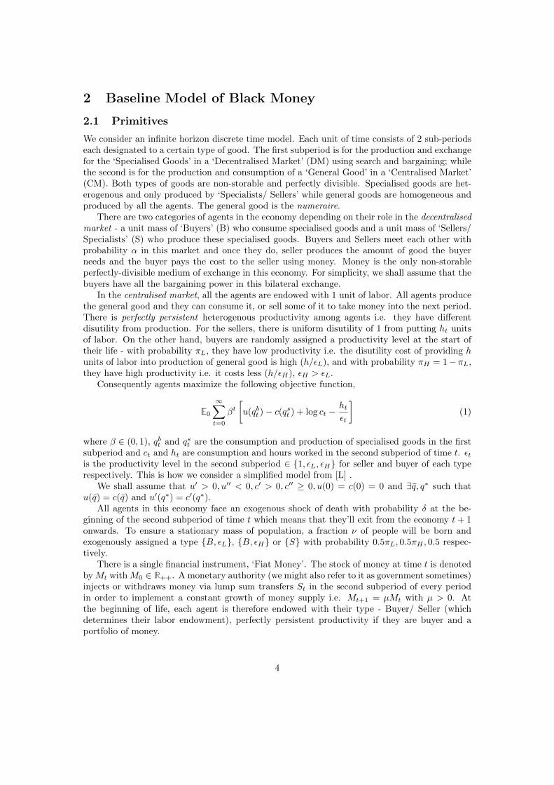
3. New Money Equilibrium where agents discard their old money or simply exchange itall for new money. In former case, demonetisation fails to punish any of the tax evaders,while in the latter the policy is most successful it can be. We call the second case as theDemonetisation Equilibrium.
Figure 8: Monetary Equilibria
µOτ0
µNτL
βεLπLfL
∆φτ+1
C
βεHπHfC
∆φτ+1
NC
βεHπLξNC
∆φτ+1
New MoneyEquilibrium
φOτ+i = 0 ∀i ≥ 0
Old MoneyEquilib-
rium as long
as¯µO, µO ≤ µN
Money LaunderingEquilibrium
DemonetisationEquilibrium
Going forward from time τ + 1, there is only old money in the system under the Old Moneyequilibrium and the new money is simply use to pay for taxes and penalty if we impose thatrequirement. The inflation in old money has to stay less than that of new money for the equi-librium to exist. In that sense, it is a fragile equilibrium because if, say, the Old Notes undergosome amount of wear and tear and consequently some tiny amount of money is lost which causes
15

higher inflation in old money. Then, the economy will transition to the new economy the momentold money’s inflation gets high enough to exceed new money’s inflation.
In case of the New Money Equilibrium (which includes the demonetisation equilibrium) andfor the area below the 45◦ line, we have only new notes going forward from τ + 1. In each ofthese cases φτ+1 = 0. This leads to the limiting case of equilibrium characterisation i.e.
Proposition 3. When the Monetary Equilibrium is such that the economy has only New Notesafter the transition period, we are in the limiting case where value of old money φOτ+i = 0 ∀i ≥ 1.In this case, the equilibrium money holdings of agent i is characterised by the following thresholdstrategy,
x∗i ,m∗Oi ,m′∗Ni s.t.
Exchange all Old money for New if µNτ ≥
βεiπif i
φNτ+1
Discard Old Money if µNτ <βεiπ
if i
φNτ+1
(36)
According to different thresholds for different agents, we have 3 possibilities (1) When allagents discard their old money and start saving in New notes at a very low money supply, highprices equilibrium, (2) When some subset of agents exchange old notes for new, others discard oldnotes. In this case, agents would prefer to launder money if they could. The price of new noteswill be lower than the previous case because the supply of new notes is higher after exchangeby some agents (3) When all the agents exchange their old notes to new, which leads to themaximum possibility of dishonest types getting caught. In this case, the price of the new notesis even lower. In fact, in a stationary equilibrium, the new notes completely replace the newnotes and the economy continues at the same inflation rate as before the transition period, withsimply a change of notes.
Finally, there are the Money Laundering Equilibrium in the red region above the 45◦ linewhere both money could stay in the economy after the transition period. In these cases, some ofthe agents continue to hold Old Notes while some exchange them for new notes. The economywould eventually move to an equilibrium with either of the notes depending on their relativeinflation in the future. This follows from the optimal money holdings decisions of the agentsfrom τ + 1 onwards summarised by the following equation,
ziτ+t =
βαεiµNτ+t − β(1− α)︸ ︷︷ ︸
Only New Notes
if µNτ+t < µOτ+t
βαεiµOτ+t − β(1− α)︸ ︷︷ ︸
Only Old Notes
if µNτ+t > µOτ+t
βαεiµτ+t − β(1− α)︸ ︷︷ ︸
Indeterminate composition
if µNτ+t = µOτ+t = µτ+t
∀t ≥ 1 (37)
In either of the equilibria, the High type dishonest agents always exist in the economy in thestationary equilibrium, the policy does not tackle the problem of ‘tax evasion’ and black moneycompletely. The laws of motion for each type fo the agents is same as before from equation19, with p, replaced by (p+ πL(x∗NC)), and we have all the type of agents still available in thiseconomy. In this sense, we are able to explain the stylised fact observed in the data (figure2). The government undertook the demonetisation policy hoping that out of the |15.4 trillion
16
of old notes, only a fraction would be deposited by the agents for exchange and a lot of richdishonest agents who might be evading tax will be compelled to discard some of their old notesto avoid punishments from getting caught. But we found that almost all of the New moneywas deposited by the agents and the New notes in circulation almost reached the same level asthe Old notes. This is indicative of the Money Laundering Equilibrium with massive amountsof money laundering as in the red area below the 45◦ line in the model. The Indian Economytransitioned to only New Money equilibrium, but with black money not completely removedfrom the system, and we explain that through our model.
5 Policy Implications
Our model of Demonetisation helps us understand the possible equilibria that emerge in theeconomy when such sudden announcements are made to get rid of black money from the system.We see that almost all the equilibria entail survival of the dishonest type of rich agents whochoose to launder money or incur a penalty by discarding new money in order to not revealtheir true taxable money holdings. Thus, a policy like Demonetisation, despite being suddenis not a complete solution to the curb black economy. Even though in our model, the agentstypes got revealed forever (i.e. they could never cheat again once caught), or they were notallowed to launder; we saw that the black money still prevailed in the system. In reality, agentstransition between types and launder money which makes the issue of black money even moregrave instead of solving it. So, there is a need for policies which involve greater direct monitoringof the agents types instead of one time demonetisation which actually cause more inconvenience(during exchange), then the benefits from mitigating the black money from the system. Somepolicies which might be more effective in reducing the size of the black economy, might be increasein p, huge and prolonged penalties to agents who are caught misreporting, and the recent surgeof digitisation which helps to track agent’s money holdings more transparently. Digitisationenforces agents to hold more income as reported, because it reduces the cost of monitoring.
6 Conclusion
In this paper, we solved a theoretical model of Black Money and Demonetisation. We foundmultiplicity of Stationary Monetary Equilibrium and we could explain some of the stylised factsobserved in the data from the Indian Economy’s demonetisation episode of Nov, 2016. Thismodel helps us understand the tradeoffs faced by rich agents in terms of evading taxes andgetting caught in an audit by the administrative authorities. It also allows us to understand theissue of Money Laundering which is prevalent in a lot of economies across the world. The model isextremely broad in its’ possibilities of any economies’ responses to such policies. Demonetisationin India is not a unique episode. Economies across the world have had policies similar to orexactly like demonetisation, eg. Nigeria (1984), Pakistan (2016), North Korea (2010), Ghana(1982) and so on. Some of the economies collapsed in response to such policies, others had aphased transition and some just overruled the policy and agents never followed it. Our model,allows for all these possibilities to emerge after such a policy.
Having understood the implications on the monetary equilibrium, one should not forget thereal economic implications of such policies as well. A sudden demonetisation of 2 of the highestdenominations notes left the Indian Economy with 86% of its’ cash in circulation invalid. It wasa massive economic shock for everyone in the economy. For an economy which has a very largeshare of cash intensive informal sector, the policy led to a huge disruption for the real activityfor the producers and consumers in these sectors. There were adverse implications on the cash
17

intensive agriculture sector, automobiles sector catering to the middle class (eg. Scooters, SmallCars), real estate black money transactions during the transition period. The agents were alsoaffected by a lot of difficulties in having to go the banks in order to deposit their old notes andthere were limits on the amount of new notes they could withdraw in cash while the rest wascredited to their bank accounts. There were long queues of depositors at the exchange windowand the disruptive transition period lasted 2 months. Hence, it would be interesting to look atthe effects of demonetisation in real output and welfare for our economy.
18
References
[LW] Lagos and Wright, JPE (2005): “A Unified Framework for Monetary Theory and PolicyAnalysis”
[EC] Economic Survey of India (2016-17) Chapter3: “Demonetisation: To Deify or Demonize?”
[MM1] Mint Street Memo No 1 (2017), Reserve Bank of India, “Demonetisation and BankDeposit Growth”, Bhupal Singh and Indrajit Roy
[MM2] Mint Street Memo No 2 (2017), Reserve Bank of India, “Financialisation of Savings intoNon-Banking Financial Intermediaries”, Manoranjan Dash, Bhupal Singh, Snehal Herwadkarand Rasmi Ranjan Behera
[MM7] Mint Street Memo No 7 (2017), Reserve Bank of India, “From Cash to Non-cash andCheque to Digital: The Unfolding Revolution in India?s Payment Systems”, Sasanka SekharMaiti
[GK] Mr. Nishant Ravindra Ghuge and CA Dr. Vivek Vasantrao Katdare, International Confer-ence on Global Trends in Engineering, Technology and Management (ICGTETM-2016): “AComparative Study of Tax Structure of India with respect to other countries”
[L] Ricardo Lagos, JPE (2013): “Moneyspots”
19
A Appendix
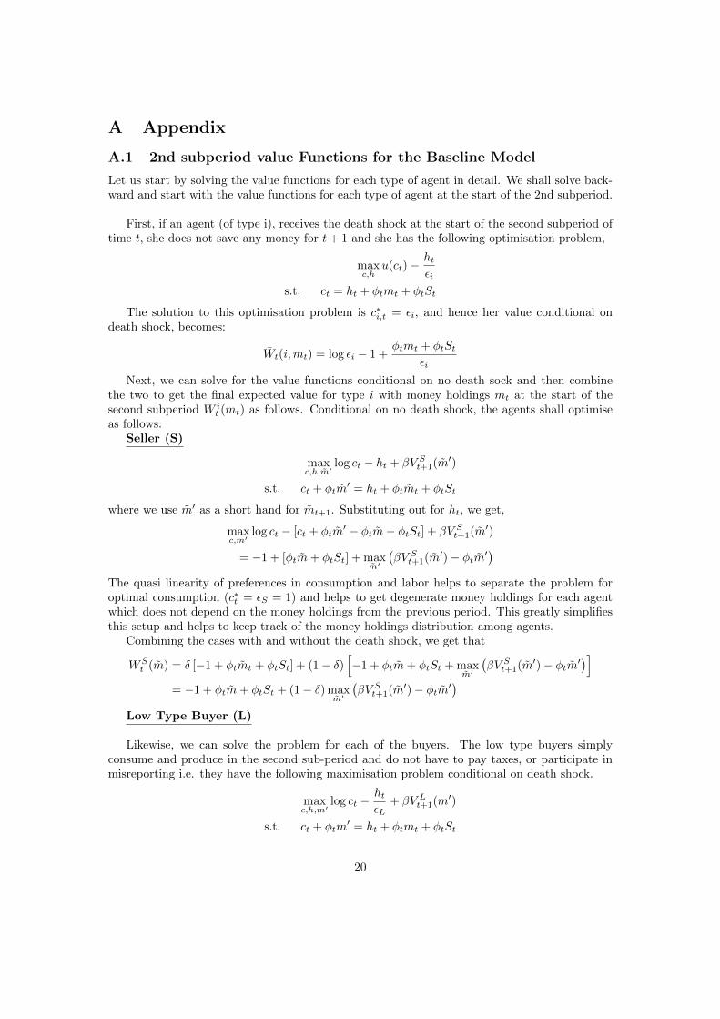
A.1 2nd subperiod value Functions for the Baseline Model
Let us start by solving the value functions for each type of agent in detail. We shall solve back-ward and start with the value functions for each type of agent at the start of the 2nd subperiod.
First, if an agent (of type i), receives the death shock at the start of the second subperiod oftime t, she does not save any money for t+ 1 and she has the following optimisation problem,
maxc,h
u(ct)−htεi
s.t. ct = ht + φtmt + φtSt
The solution to this optimisation problem is c∗i,t = εi, and hence her value conditional ondeath shock, becomes:
Wt(i,mt) = log εi − 1 +φtmt + φtSt
εi
Next, we can solve for the value functions conditional on no death sock and then combinethe two to get the final expected value for type i with money holdings mt at the start of thesecond subperiod W i
t (mt) as follows. Conditional on no death shock, the agents shall optimiseas follows:
Seller (S)
maxc,h,m′
log ct − ht + βV St+1(m′)
s.t. ct + φtm′ = ht + φtmt + φtSt
where we use m′ as a short hand for mt+1. Substituting out for ht, we get,
maxc,m′
log ct − [ct + φtm′ − φtm− φtSt] + βV St+1(m′)
= −1 + [φtm+ φtSt] + maxm′
(βV St+1(m′)− φtm′
)The quasi linearity of preferences in consumption and labor helps to separate the problem foroptimal consumption (c∗t = εS = 1) and helps to get degenerate money holdings for each agentwhich does not depend on the money holdings from the previous period. This greatly simplifiesthis setup and helps to keep track of the money holdings distribution among agents.
Combining the cases with and without the death shock, we get that
WSt (m) = δ [−1 + φtmt + φtSt] + (1− δ)
[−1 + φtm+ φtSt + max
m′
(βV St+1(m′)− φtm′
)]= −1 + φtm+ φtSt + (1− δ) max
m′
(βV St+1(m′)− φtm′
)Low Type Buyer (L)
Likewise, we can solve the problem for each of the buyers. The low type buyers simplyconsume and produce in the second sub-period and do not have to pay taxes, or participate inmisreporting i.e. they have the following maximisation problem conditional on death shock.
maxc,h,m′
log ct −htεL
+ βV Lt+1(m′)
s.t. ct + φtm′ = ht + φtmt + φtSt
20
=⇒ maxc,m′
log ct −1
εL[ct + φtm
′ − φtmt − φtSt] + βV Lt+1(m′)
= log εL − 1 +φtmt + φtSt
εL+ max
m′
[βV Lt+1(m′)− φtm
′
εL
]Combining the cases with and without death shock, we get that
WLt (mt) = log εL − 1 +
φtmt + φtStεL
+ (1− δ) maxm′
[βV Lt+1(m′)− φtm
′
εL
]High type Caught Buyer (C)
The high type ‘Caught’ buyer has a similar problem as that of the low type with no mis-reporting incentive, except she has to pay taxes (either because she chose to be honest in reportingher type or she was caught in some previous time period and her true type is revealed forever).So, she solves the following,
maxc,h,m′
log ct −htεH
+ βV Ct+1(m′)
s.t. ct + φtm′ = ht + φtmt − T + φtSt
=⇒ maxc,m′
log ct −1
εH[ct + φtm
′ − (φtmt − T)− φtSt] + βV Ct+1(m′)
= log εH − 1 +(φtmt − T) + φtSt
εH+ max
m′
[βV Ct+1(m′)− φtm
′
εH
]Combining the cases with and without death shock, we get that
WCt (mt) = log εH − 1 +
(φtmt − T) + φtStεH
+ (1− δ) maxm′
[βV Ct+1(m′)− φtm
′
εH
]High type Not Caught Buyer (NC)
Finally, the high type ‘Not Caught’ buyer has an additional decision to make: whether toreport her true type and pay taxes, or to continue to misreport and take the chances of gettingcaught with some probability (p) of government audit. Hence, her maximisation problem alsoinvolves reporting strategy, and using the same steps as above, simplifies to the following:
=⇒ WNCt (mt) = log εH − 1 +
φm+ φStεH
+ 1ε=εH
[−TεH
+ (1− δ) maxm′
(βV Ct+1(m′)− φm′
εH
)]+
1ε=εL
[p
(−PεH
+ (1− δ) maxm′
[βV Ct+1(m′)− φm′
εH
])+ (1− p)
((1− δ) max
m′
[βV NCt+1 (m′)− φm′
εH
])]
A.2 Nash Bargaining Problem for the Baseline Model
We know that the buyer maximises as follows:
maxqB ,d≤m
ut(qBt (mt, εi, mt)) +W i
t (mt − d(mt, εi, mt))−W it (mt)
subject to − ct(qBt (mt, εi, mt)) +WSt (mt + d(mt, εi, mt))−WS
t (mt) ≥ 0
21
Using the quasi linearity result in 8, we can simplify this as follows,
maxqB ,d≤m
ut(qBt (mt, εi, mt))−
φtd(mt, εi, mt)
εi
subject to − ct(qBt (mt, εi, mt)) + φtd(mt, εi, mt) ≥ 0
Since the buyer has all the bargaining power and her utility is increasing in the quantity ofspecialised good consumed, the seller’s participation constraint binds, i.e. the buyer only paysenough money to the seller to compensate her for the cost of producing the good i.e.
φtd(mt, εi, mt) = ct(qBt (mt, εi, mt))
=⇒ maxqB ,d≤m
ut(qBt (mt, εi, mt))−
ct(qBt (mt, εi, mt))
εi
Define q∗t (m, εi) ={q|u′t(q) =
c′t(q)εi
}, then the optimal decision of the Nash Bargaining is,
qBt (mt, εi) =
{q∗t (mt, εi) if ct(q
∗t (mt, εi)) ≤ φtmt
{qt|ct(qt(mt, εi)) = φtmt} otherwise
and for the payment,
dt(mt, εi) =
ct(q
∗t (mt, εi))
φtif ct(q
∗t (mt, εi)) ≤ φtmt
mt otherwise
Value functions at the start of the 1st subperiod
With the solution to the Nash Bargaining, we now know the flow payoff during the firstsubperiod and we can get the value functions V it (mt) for each type i of the agent as follows:
Seller (S)
With probability απL, the seller meets the low type buyer, produces the good as demanded,and gets the continuation payoff after receiving the payment, with απH , she meets the high typebuyer and with 1−α, she does not meet a counter-party to produce and exchange the specialisedgood.
V St (mt) = απL[−ct(qBt (mt, εL)) +WS
t (mt + d(mt, εL))]
+
απH[−ct(qBt (mt, εH)) +WS
t (mt + d(mt, εH))]
+ (1− α)WSt (mt)
Since, the seller gets no gain from trade in the DM, from the above bargaining solution whereφtdt = ct(q
Bt ) always, we get that her value at the start of the period, is just equal to her payoff
at the start of the second subperiod,
V St (mt) = WSt (mt) = φtmt +WS
t (0)
In this sense, the seller in this model is more like a facilitating agent that supports the moreinteresting side of heterogenous buyers.
22
Low Type Buyers (L)
For the low type buyers, they only get flow payoff in the DM, if they meet a seller withprobability α,
V Lt (mt) = α[ut(q
Bt (mt, εL)) +WL
t (mt − d(mt, εL))]
+ (1− α)WLt (mt)
= α
[ut(q
Bt (mt, εL))− φtd(mt, εL))
εL
]+φtmt
εL+WL
t (0)
= α
[ut(q
Bt (mt, εL))− ct(q
Bt (mt, εL))
εL
]+φtmt
εL+WL
t (0)
High Type Buyers i ∈ {C,NC}
Likewise for the high type buyer whether of not she has been caught in the past, we get thefollowing value functions at the start of the first subperiod,
V it (mt) = = α
[ut(q
Bt (mt, εH))− ct(q
Bt (mt, εH))
εH
]+φtmt
εH+W i
t (0)
A.3 Guess and Verify solution for threshold value of audit probability
We know that the value function at the start of the second subperiod, for the high type NCbuyer, when she decides on her reporting strategy is as follows:
WNCt (mt) = log εH − 1 +
φtmt + φStεH
+ 1ε=εH
[−TεH
+ (1− δ) maxm′
(βV Ct+1(m′)− φm′
εH
)]+
1ε=εL
[p
(−PεH
+ (1− δ) maxm′
βV Ct+1(m′)− φm′
εH
)+ (1− p)
((1− δ) max
m′βV NCt+1 (m′)− φm′
εH
)]We guess that the value of p is such that the agent prefers to misreport than to turn honest
i.e.
p
(−PεH
+ (1− δ) maxm′
βV Ct+1(m′)− φm′
εH
)+ (1− p)
((1− δ) max
m′βV NCt+1 (m′)− φm′
εH
)≥ −TεH
+ (1− δ) maxm′
(βV Ct+1(m′)− φm′
εH
)(38)
Under the guess, we know that her value function is as follows,
WNCt (mt) = log εH − 1 +
φtmt + φStεH
+
[p
(−PεH
+ (1− δ) maxm′
βV Ct+1(m′)− φm′
εH
)+
(1− p)(
(1− δ) maxm′
βV NCt+1 (m′)− φm′
εH
)]Next, we solve for the optimal value of money holdings for each type of agent under the guess.
Let us define
Γit(mt) ≡ ut(qBt (mt, εi))−ct(q
Bt (mt, εi))
εi
23
Also, let us solve for the derivative of Γit(mt) w.r.t. mt as follows:
∂Γit(mt)
∂mt=
(∂Γit(mt)
∂qBt
)∂qBt∂mt
=
[u′t(q
Bt )− c′t(q
Bt )
εi
]∂qBt∂mt
From, 10, we get that
∂Γit(mt)
∂mt=
0 if ct(q∗t (mt, εi)) ≤ φtmt[
u′t(q)−c′t(q)
εi
]∂q
∂mtotherwise
using the definition of q∗ s.t. u′(q∗) = c′(q∗)εi
. Also, using the definition of q, we get that∂q
∂mt=
φtc′t(qt(mt, εi))
. Substituting this in the second case above, we get that
∂Γit(mt)
∂mt=
0 if ct(q∗t (mt, εi)) ≤ φtmt[
u′t(qt(mt, εi))
c′t(qt(mt, εi))− 1
εi
]φt otherwise
With this notation in hand, let us solve for the optimal money holding decision for each typeof agent.
Seller (S)
First for the seller, she faces the following optimisation problem once we substitute for V St+1
into WSt ,
WSt (mt) = −1 + φtm+ φtSt + (1− δ) max
m′
(β(φt+1m
′ +WSt+1(0)
)− φtm′
)This leads to the following first order condition for money holdings,
{m′S} : (1− δ)(βφt+1 − φt)
We shall look at the stationary equilibrium for this economy i.e. φtMt = φt+1Mt+1 in
equilibrium. This implies φtφt+1
= Mt+1
Mt= µ. Moreover, we shall only consider the case when
β ≤ µ, else all agents would want to hold infinite amount of money and that would not besupported by market clearing in equilibrium. Further, we shall look at a stationary equilibrium inwhich all agents hold a constant amount of real money holdings φtm
it = zi over time. Considering
all this, we get from the above FOC for seller, that
β − µ < 0 =⇒ m′S = 0 =⇒ zS = 0
Low Type Buyer (L)
The low type buyer has the following optimisation problem once we substitute for the valuefunction V Lt+1(mt+1) from next period into WL
t (mt) and use the definition of ΓLt+1(mt+1) asfollows,
WLt (mt) = log εL − 1 +
φtmt + φtStεL
+ (1− δ) maxm′
[β
(αΓLt+1(m′) +
φt+1m′
εL+WL
t+1(0)
)− φtm
′
εL
]
24

This implies the following FOC for money holdings. We rule out the case in which∂ΓLt+1(m′)
∂m′=
0, i.e. qBt = q∗, because then we get that the agents choice of money holdings depend onβ − µεL
< 0, i.e. she holds 0 money but consumes optimal amount of specialised good next period
(contradiction). This shows that the buyer is only able to consume less than her optimal levelof specialised good, and she exhausts all her money holdings in doing so, i.e. each buyer shallonly be able to demand q units of specialised good in the DM.
{m′L} : (1− δ)[β
(α∂ΓLt+1(m′)
∂m′+φt+1
εL
)− φtεL
]≤ 0
=⇒ (1− δ)[β
(α
[u′t+1(qt+1(m′, εL))
c′t+1(qt+1(m′, εL))− 1
εL
]φt+1 +
φt+1
εL
)− φtεL
]≤ 0
=⇒ βα
[(u′
c′
)t+1
(qt+1(m′, εL))
]φt+1 +
β(1− α)φt+1
εL− φtεL≤ 0
Assuming that we have an interior solution for money holdings, and using the definition of q,we get the FOC, which leads to some degenerate value of money holdings m′L(φt+1, β, α, εL, µ)depending on the functional form of u, and c, such that zL = φt+1m
′ is constant and solves thefollowing FOC:
{zL} :
{u′c′
}t+1
(c−1t+1(φt+1m
′L︸ ︷︷ ︸zL
)
=µ− β(1− α)
βαεL
=⇒ zL = ct+1
({u′
c′
}−1
t+1
[µ− β(1− α)
βαεL
])
If for example, we have ut(qBt ) = log qBt , and ct(q
Bt ) = cqBt , we get that
zL =βαεL
µ− β(1− α)
High Type Caught Buyer (C)
Using the exact same steps as for the low type, it is easy to show that the money holdingsfor the high type Caught buyer can be solved from the following FOC, which for the case of logutility and linear cost is as follows:
zC = ct+1
({u′
c′
}−1
t+1
[µ− β(1− α)
βαεH
])=⇒ zC =
βαεHµ− β(1− α)
High Type Not Caught Buyer (NC)
For this type, we look at the value function at the start of the second subperiod, and substitutefor the optimal value function after getting caught, and the value function for the NC type V NCt+1
as follows,
25

WNCt (mt) = log εH − 1 +
φtmt − pP + φStεH
+ (1− δ)[p
(βV Ct+1(m′C)− φtm
′C
εH
)+
(1− p)(
maxm′
β
[αΓNCt+1(m′) +
φt+1m′
εH+WNC
t+1 (0)
]− φtm
′
εH
)]
Getting the FOC for money holdings,
{m′NC} : (1− δ)(1− p)(β
[α∂ΓNCt+1(m′)
∂m′+φt+1
εH
]− φtεH
)= (1− δ)(1− p)
(β
[α∂ΓNCt+1(m′)
∂m′+φt+1
εH
]− φtεH
)Using the same steps as before, we get that the high type not caught holds the same amount
of money holdings as the high type caught buyer but works less since she does not have to paytaxes.
zNC = ct+1
({u′
c′
}−1
t+1
[µ− β(1− α)
βαεH
])=⇒ zNC =
βαεHµ− β(1− α)
Having solved for the optimal values of real money holdings under the guess, we can go backto the condition in 38 and verify when the guess is satisfied in equilibrium. From 38, and oursolution,
p
(−PεH
+ (1− δ)[βV Ct+1(m′C)− φtm
′C
εH
])+ (1− p)
((1− δ)
[βV NCt+1 (m′NC)− φtm
′NC
εH
])≥ −TεH
+ (1− δ)[βV Ct+1(m′C)− φtm
′C
εH
]=⇒ p
[PεH
+ (1− δ)[(βV NCt+1 (m′NC)− φtm
′NC
εH
)−(βV Ct+1(m′C)− φtm
′C
εH
)]]≤ TεH
+ (1− δ)[(βV NCt+1 (m′NC)− φtm
′NC
εH
)−(βV Ct+1(m′C)− φtm
′C
εH
)]Since, zC = zNC , we can simplify this to,
p
[PεH
+ (1− δ)β(V NCt+1 (m′NC)− V Ct+1(m′C)
)]≤ TεH
+ (1− δ)β(V NCt+1 (m′NC)− V Ct+1(m′C)
)Next, note that V NCt+1 (m′NC) − V Ct+1(m′C) = WNC
t+1 (0) −WCt+1(0), since they have the same
amount of optimal money holdings, and from (6) - (7), we can substitute that out to get thefollowing within the framework of a stationary equilibrium,
WNCt+1 (0)−WC
t+1(0) =−pP + TεH
+ (1− δ)(1− p)β(WNCt+2 (0)−WC
t+2(0))
=⇒ WNC −WC =−pP + T
[1− (1− δ)(1− p)β]εH
26
Going back, to the inequality, we can substitute this out to get,
p
[PεH
+ (1− δ)β(
−pP + T[1− (1− δ)(1− p)β]εH
)]≤ TεH
+ (1− δ)β(
−pP + T[1− (1− δ)(1− p)β]εH
)=⇒ pP− T
εH≤ (1− p)(1− δ)β
(−pP + T
[1− (1− δ)(1− p)β]εH
)=⇒ 0 ≤ T− pP
εH
[1 +
(1− p)(1− δ)β[1− (1− δ)(1− p)β]
]
=⇒ 0 ≤ T− pPεH
1
[1− (1− δ)(1− p)β]︸ ︷︷ ︸+ve
=⇒ p ≤ T
P≡ p∗
A.4 Value functions for the Model with Demonetisation
First let us simplify the generic second subperiod value function incorporating for the deathshock. The agents again have the same optimisation problem upon death, i.e.
maxc,h
log cτ −hτεi
s.t. cτ = hτ + φOτ mOτ + φNτ m
Nτ + φNτ Sτ
=⇒ W iτ (mO,mN ) = log εi − 1 +
φOτ mOτ + φNτ m
Nτ + φNτ Sτ
εi
In case of no death shock, the agents also have same problem as before with the continuationvalues being U ’S instead of V ’s now.
maxc,h,m′O,m′N
log cτ −hτεi
+ U iτ (m′O,m′N )
s.t. cτ + φOτ m′Oτ + φNτ m
′Nτ = hτ + φOτ m
Oτ + φNτ m
Nτ + φNτ Sτ
= log εi − 1 +φOτ m
Oτ + φNτ m
Nτ + φNτ Sτ
εi+ maxm′O,m′N
U iτ (m′O,m′N )− φOτ m′Oτ + φNτ m
′Nτ
εi
Combining the 2, we get W iτ (mO,mN ) = δ(W i
τ (mO,mN )) + (1 − δ)(above value), which weshall now specify in detail for each type of agents.
Seller (S)
At the start of the exchange period, agents come with certain holdings of new and old money.They choose how much of the old money (0 ≤ x ≤ m′O), should they convert into new money,given they can gain for the higher value of new money but also get caught and penalised if theytry to launder money.
USτ (m′O,m′N ) = max0≤x≤m′O
β[V Sτ+1(m′O − x,m′N + x)− πS(x)fS
]
27

Using the above explanation,
WSτ (mO,mN ) = −1 +
(φOτ m
O + φNτ mN + φNτ Sτ
)+ (1− δ) max
m′O,m′NUSτ (m′O,m′N )−
(φOτ m
′O + φNτ m′N)
=(φOτ m
O + φNτ mN)
+WSτ (0, 0)
Note that the quasi linearity of W still holds and we use it in exactly the same way in solving forthe terms of trade in DM. Also, since the bargaining problem is essentially the same as beforewith φtmt replaced by φOt m
Ot + φNt m
Nt , and the seller got no flow payoff from Nash Bargaining,
we get
V Sτ (mO,mN ) = WSτ (mO,mN )
Solving for the optimal amount of money holdings for the seller, using the above value func-tions, we get
USτ (m′O,m′N ) = max0≤x≤m′O
β[WSτ+1(m′O − x,m′N + x)− πS(x)fS
]FOC for {x} is decreasing in x using the assumption that π′ > 0, we get the following
threshold strategy,
Let xS : β[(φNτ+1 − φOτ+1)− π′S(x)fS
]= 0
=⇒ x∗(m′O) = max{0,min{m′O, xS}}
i.e. the Seller shall exchange all her money holdings upto xS . Next, we substitute this back intothe period before i.e. W , and solve for the optimal amount of money holdings of Old and NewMoney as follows:
WSτ (mO,mN ) = −1 +
(φOτ m
O + φNτ mN + φNτ Sτ
)+ (1− δ) max
m′O,m′N[β[WSτ+1(m′O − x∗(m′O),m′N + x∗(m′O))− πS(x∗(m′O))fS
]]−(φOτ m
′O + φNτ m′N)
FOC for {m′O}, {m′N}:
{m′O} : β
[φOτ+1
(1− ∂x∗(m′O)
∂m′O
)+ φNτ+1
(∂x∗(m′O)
∂m′O
)− π′S(x∗(m′O))
(∂x∗(m′O)
∂m′O
)fS]− φOτ
=
{β[φNτ+1 − π′S(m′O)fS
]− φOτ when m′O ≤ xS
βφOτ+1 − φOτ when xS ≤ m′O
{m′N} : βφNτ+1 − φNτ
Assume that β ≤ µNτ , β ≤ µOτ =⇒
m′OS ∈ [0, xS ] : β[φNτ+1 − π′S(m′OS )fS
]− φOτ = 0
m′NS = 0
This gives us the optimal money holdings decision for the sellers.
28
Low type buyer (L)
We follow the same steps as for the Seller, to get the value functions for the low type buyer.First, she chooses the exchange amount at time τ , she reports i = L, i.e. she is monitored withprobability πL, and if she deposits more money than what she holds, i.e. in order to launder,the punishment kicks in and stops her. Further, her value functions at the start of the first andsecond subperiod are also derived as follows:
ULτ (m′O,m′N ) = max0≤x≤m′O
β[V Lτ+1(m′O − x,m′N + x)− πL(x)fL
]WLτ (mO,mN ) = log εL − 1 +
(φOτ m
O + φNτ mN + φNτ Sτ
εL
)+
(1− δ) maxm′O,m′N
{ULτ (m′O,m′N )−
(φOτ m
′O + φNτ m′N
εL
)}=
(φOτ m
O + φNτ mN
εL
)+WL
τ (0, 0)
V Lτ+1(m′O,m′N ) = α[ΓLτ+1(m′O,m′N )
]+WL
τ+1(m′O,m′N )
where ΓLτ+1(m′O,m′N ) =
[uτ+1(qbτ+1(m′O,m′N , εL))−
cτ+1(qbτ+1(m′O,m′N , εL))
εL
]is the modi-
fied version of Γ with a portfolio of old and new notes.
We start with solving for the optimal amount of exchange for a given value of money holdingsof old notes and new notes by substituting out for the Vτ+1
=⇒ ULτ (m′O,m′N ) = max0≤x≤m′O
β[αΓLτ+1(m′O − x,m′N + x) +WL
τ+1(m′O − x,m′N + x)− πL(x)fL]
FOC for {x} : β
[α∂ΓLτ+1(m′O − x,m′N + x)
∂x+
(φNτ+1 − φOτ+1
εL
)− π′L(x)fL
]We know that, under our utility and cost functions, where in we assumes u(q) = log q, c(q) =
cq,
∂ΓLτ+1(m′O − x,m′N + x)
∂m′O=
[1
φ.m− 1
εL
]φOτ+1,
∂ΓLτ+1(m′O − x,m′N + x)
∂m′N=
[1
φ.m− 1
εL
]φNτ+1
with φ.m = φOτ+1(m′O − x) + φNτ+1(m′N + x), =⇒ the following FOC decreasing in x.Consequently, we shall get a threshold strategy also for the poor buyer. Let xL(m′O,m′N ) besuch that,
β
[α
((φNτ+1 − φOτ+1)
φOτ+1m′O + φNτ+1m
′N + (φNτ+1 − φOτ+1)xL
)+ (1− α)
(φNτ+1 − φOτ+1
εL
)− π′L(xL)fL
]= 0
=⇒ x∗(m′O,m′N ) = max{0,min{m′O, xL(m′O,m′N )}}
Again, once we solve for the optimal value of exchange as a function of money holdings, wecan move back to the value function W at the start of the second subperiod as follows,
29
=⇒ WLτ (mO,mN ) = log εL − 1 +
(φOτ m
O + φNτ mN + φNτ Sτ
εL
)+ (1− δ) max
m′O,m′N
{β[αΓLτ+1(m′O − x∗L,m′N + x∗L)
+WLτ+1(m′O − x∗L,m′N + x∗L)− πL(x∗)fL
]−(φOτ m
′O + φNτ m′N
εL
)}Getting our first order conditions for money holdings,
{m′O} : β
[α
(∂ΓLτ+1(·)∂m′O
{1− ∂x∗(·)
∂m′O
}+∂ΓLτ+1(·)∂m′N
{∂x∗(·)∂m′O
})+φOτ+1
εL
{1− ∂x∗(·)
∂m′O
}+φNτ+1
εL
{∂x∗(·)∂m′O
}−π′L(x∗)
{∂x∗(·)∂m′O
}fL]− φOτεL
{m′N} : β
[α
(∂ΓLτ+1(·)∂m′O
{−∂x
∗(·)∂m′N
}+∂ΓLτ+1(·)∂m′N
{1 +
∂x∗(·)∂m′N
})+φOτ+1
εL
{−∂x
∗(·)∂m′N
}+φNτ+1
εL
{1 +
∂x∗(·)∂m′N
}−π′L(x∗)
{∂x∗(·)∂m′N
}fL]− φNτεL
Simplifying and substituting for the partial derivatives under our example with log utility andconstant marginal cost of production, we get the following,
{m′O} :
β[
αφOτ+1
φOτ+1m′O+φNτ+1m
′N+(φNτ+1−φOτ+1)xL+
(1−α)φOτ+1
εL
]− φOτ
εLif m′O > xL ≥ 0
β[
α(m′N+m′O)
+(1−α)φNτ+1
εL− πLfL
]− φOτ
εLif m′O ≤ xL
{m′N} :
β[
α(m′N+m′O)
+(1−α)φNτ+1
εL
]− φNτ
εLif xL ≥ m′O
β[
αφNτ+1
φOτ+1m′O+φNτ+1m
′N+(φNτ+1−φOτ+1)xL+
(1−α)φNτ+1
εL
]− φNτ
εLif xL ≤ m′O
High type Caught Buyer (C)
The value functions for the high type buyer whose type is already revealed is as follows. Herreposted type is i = H, and the corresponding fine fC .
UCτ (m′O,m′N ) = max0≤x≤m′O
β[V Cτ+1(m′O − x,m′N + x)− πH(x)fC
]WCτ (mO,mN ) = log εH − 1 +
(φOτ m
O + φNτ mN − T + φNτ SτεH
)+
(1− δ) maxm′O,m′N
{UCτ (m′O,m′N )−
(φOτ m
′O + φNτ m′N
εH
)}=
(φOτ m
O + φNτ mN
εH
)+WC
τ (0, 0)
V Cτ+1(m′O,m′N ) = αΓHτ+1(m′O,m′N ) +WCτ+1(m′O,m′N )
where ΓHτ+1(m′O,m′N ) =
[uτ+1(qBτ+1(m′O,m′N , εH))−
cτ+1(qBτ+1(m′O,m′N , εH))
εH
]
30
Substituting for Vτ+1 in Uτ , we get
=⇒ UCτ (m′O,m′N ) = max0≤x≤m′O
β[αΓHτ+1(m′O − x,m′N + x) +WC
τ+1(m′O − x,m′N + x)− πH(x)fC]
This leads to the following First order condition for exchange amount,
{x} : β
[α∂ΓHτ+1(m′O − x,m′N + x)
∂x+
(φNτ+1 − φOτ+1
εH
)− π′H(x)fC
]For out choice of utility and cost functions,
∂ΓHτ+1(m′O − x,m′N + x)
∂m′O=
[1
φ.m− 1
εH
]φOτ+1,
∂ΓLτ+1(m′O − x,m′N + x)
∂m′N=
[1
φ.m− 1
εH
]φNτ+1
with φ.m = φOτ+1(m′O − x) + φNτ+1(m′N + x). =⇒ the following FOC decreasing inx. Consequently, we shall get a threshold strategy also for the high type caught buyer. LetxC(m′O,m′N ) be such that,
β
[α
((φNτ+1 − φOτ+1)
φOτ+1m′O + φNτ+1m
′N + (φNτ+1 − φOτ+1)xC
)+ (1− α)
(φNτ+1 − φOτ+1
εH
)− π′H(xC)fC
]= 0
=⇒ x∗C(m′O,m′N ) = max{0,min{m′O, xC(m′O,m′N )}}
Substituting this back into the value function at the start of the second subperiod,
WCτ (mO,mN ) = log εH − 1 +
(φOτ m
O + φNτ mN − T + φNτ SτεH
)+ (1− δ) max
m′O,m′N{β[αΓHτ+1(m′O − x∗,m′N + x∗) +WC
τ+1(m′O − x∗,m′N + x∗)− πH(x∗)fC]−(φOτ m
′O + φNτ m′N
εH
)}
This leads to the following first order conditions for money holdings,
{m′O} : β
[α
(∂ΓHτ+1(·)∂m′O
{1− ∂x∗(·)
∂m′O
}+∂ΓHτ+1(·)∂m′N
{∂x∗(·)∂m′O
})+φOτ+1
εH
{1− ∂x∗(·)
∂m′O
}+φNτ+1
εH
{∂x∗(·)∂m′O
}−π′H(x∗)
{∂x∗(·)∂m′O
}fC]− φOτεH
{m′N} : β
[α
(∂ΓHτ+1(·)∂m′O
{−∂x
∗(·)∂m′N
}+∂ΓHτ+1(·)∂m′N
{1 +
∂x∗(·)∂m′N
})+φOτ+1
εH
{−∂x
∗(·)∂m′N
}+φNτ+1
εH
{1 +
∂x∗(·)∂m′N
}−π′H(x∗)
{∂x∗(·)∂m′N
}fC]− φNτεH
which can be simplified as follows,
{m′O} : =
β[
α(m′N+m′O)
+(1−α)φNτ+1
εH− π′H(m′O)fC
]− φOτ
εHif 0 ≤ m′O ≤ xC
β[
αφOτ+1
φOτ+1m′O+φNτ+1m
′N+(φNτ+1−φOτ+1)xC+
(1−α)φOτ+1
εH
]− φOτ
εHif xC < m′O
{m′N} : =
β[
α(m′N+m′O)
+(1−α)φNτ+1
εH
]− φNτ
εHif 0 ≤ m′O ≤ xC
β[
αφNτ+1
φOτ+1m′O+φNτ+1m
′N+(φNτ+1−φOτ+1)xC+
(1−α)φNτ+1
εH
]− φNτ
εHif xC < m′O
31
High type Not Caught Buyer (NC)
The high type not caught buyer is the most interesting one, since she faces the tradeoff ofgetting her type revealed in case she is caught exchanging more money than her reported typecould have. The in the event that she gets audited for exchange, her penalty is much higher, andher value function is as follows.
UNCτ (m′O,m′N ) = max0≤x≤m′O
πL(x)[β(V Cτ+1(m′O − x,m′N + x)− fNC)
]+
(1− πL(x))[βV NCτ+1 (m′O − x,m′N + x)
]WNCτ (mO,mN ) = log εH − 1 +
(φOτ m
O + φNτ mN + φNτ Sτ
εH
)+ max
ε[1ε=εH
{−TεH
+ (1− δ) maxm′O,m′N
(UCτ (m′O,m′N )− φOτ m
′O + φNτ m′N
εH
)}+
1ε=εL
{p
(−PεH
+ (1− δ) maxm′O,m′N
(UCτ (m′O,m′N )− φOτ m
′O + φNτ m′N
εH
))+
(1− p)(
(1− δ) maxm′O,m′N
(UNCτ (m′O,m′N )− φOτ m
′O + φNτ m′N
εH
))}]V NCτ+1 (m′O,m′N ) = αΓHτ+1(m′O,m′N ) +WNC
τ+1(m′O,m′N )
where ΓHτ+1(m′O,m′N ) =
[uτ+1(qbτ+1(m′O,m′N , εH))−
cτ+1(qbτ+1(m′O,m′N , εH))
εH
]Substituting, for tomorrow’s value function Vτ+1 into U, and assuming that the agent prefers
to still misreport her type when she is not caught, we get the following,
=⇒ UNCτ (m′O,m′N ) = max0≤x≤m′O
πL(x)β[αΓHτ+1(m′O − x,m′N + x) +WC
τ+1(m′O − x,m′N + x)− fNC]
+(1− πL(x))β[αΓHτ+1(m′O − x,m′N + x) +WNC
τ+1(m′O − x,m′N + x)]
This leads to the following first order condition for {x}:
β
[α∂ΓHτ+1(m′O − x,m′N + x)
∂x+φNτ+1 − φOτ+1
εH
]+
π′L(x)β[WCτ+1(m′O − x,m′N + x)− fNC −WNC
τ+1(m′O − x,m′N + x)]
I solve the baseline model for the case with both old and new money and it is easy to showthat the high type caught and not caught agents hold the same amount of money holdings goingforward from τ + 1 onwards, so we can easily subtract the 2 values as follows:
WCτ+1(m′O,m′N )−WNC
τ+1(m′O,m′N ) =−TεH− p−P
εH+ (1− p)(1− δ)β[WC
τ+2 −WNCτ+2]
=1
1− (1− p)(1− δ)βpP− TεH
32
Substituting this back in the above FOC, we get:
{x} : β
[α
((φNτ+1 − φOτ+1)
φOτ+1m′O + φNτ+1m
′N + (φNτ+1 − φOτ+1)x
)+
(1− α)(φNτ+1 − φOτ+1)
εH
]− π′L(x)β
[1
1− (1− p)βT− pPεH
+ fNC]
Again, this is decreasing in x, which implies a unique threshold value xNC(m′O,m′N ) such that
β
[α
((φNτ+1 − φOτ+1)
φOτ+1m′O + φNτ+1m
′N + (φNτ+1 − φOτ+1)xNC
)+
(1− α)(φNτ+1 − φOτ+1)
εH
]− π′L(xNC)β
[1
1− (1− p)βT− pPεH
+ fNC]
= 0
=⇒ x∗ = max{0,min{m′O, xNC(m′O,m′N )}}
Substituting this back to get the optimal value at the start of the exchange window whichwill also be the continuation value to the second subperiod value function.
=⇒ UNCτ (m′O,m′N ) = πL(x∗)β[αΓHτ+1(m′O − x∗,m′N + x∗) +WC
τ+1(m′O − x∗,m′N + x∗)− fNC]
+(1− πL(x∗))β[αΓHτ+1(m′O − x∗,m′N + x∗) +WNC
τ+1(m′O − x∗,m′N + x∗)]
Next, we want the threshold value of pτ at time τ to be also such that the agent does notwant to reveal her type in the Report and Verify window, i.e. we solve for the threshold value ofp∗ also for time τ ,
{−TεH
+ maxm′O,m′N
(UCτ (m′O,m′N )− φOτ m
′O + φNτ m′N
εH
)}≤{
p
(−PεH
+ maxm′O,m′N
(UCτ (m′O,m′N )− φOτ m
′O + φNτ m′N
εH
))+
(1− p)(
maxm′O,m′N
(UNCτ (m′O,m′N )− φOτ m
′O + φNτ m′N
εH
))}
=⇒ pP− TεH
≤ (1− p){
maxm′O,m′N
(UNCτ (m′O,m′N )− φOτ m
′O + φNτ m′N
εH
)−
maxm′O,m′N
(UCτ (m′O,m′N )− φOτ m
′O + φNτ m′N
εH
)}Now, we know the solution to get UCτ , but we should solve for UNCτ under such guess for
probability of monitoring. This implies, the agent chooses to never reveal her type.
33
Under the guess, we get the following value function at the start of the second subperiod,
WNCτ (mO,mN ) = log εH − 1 +
(φOτ m
O + φNτ mN + φNτ Sτ
εH
)+{
p
(−PεH
+ (1− δ) maxm′O,m′N
(UCτ (m′O,m′N )− φOτ m
′O + φNτ m′N
εH
))+
(1− p)(
(1− δ) maxm′O,m′N
(UNCτ (m′O,m′N )− φOτ m
′O + φNτ m′N
εH
))}= log εH − 1 +
(φOτ m
O + φNτ mN + φNτ Sτ
εH
)+{
p
(−PεH
+ (1− δ)(β[V Cτ+1(m′OC − x∗C ,m′NC + x∗C)− πH(x∗C)fC ]− φOτ m
′OC + φNτ m
′NC
εH
))+ (1− p)(1− δ) max
m′O,m′N
((πL(x∗NC)
[β(V Cτ+1(m′O − x∗NC ,m′N + x∗NC)− fNC)
]+
(1− πL(x∗NC))[βV NCτ+1 (m′O − x∗NC ,m′N + x∗NC)
]− φOτ m
′O + φNτ m′N
εH
))}So, we can get the FOC for the money holdings of the high type not caught buyer in the last
period when exchange is possible, by taking the first order conditions for m′O and m′N in theabove value function.
{m′O} :
(π′L(x∗NC)
∂x∗(·)∂m′O
)β[V Cτ+1(·)− fNC − V NCτ+1 (·)
]+ πL(x∗NC)β
[∂V Cτ+1(·)∂m′O
{1− ∂x∗NC(·)
∂m′O
}+∂V Cτ+1(·)∂m′N
{∂x∗NC(·)∂m′O
}]+ (1− πL(x∗NC))β
[∂V NCτ+1 (·)∂m′O
{1− ∂x∗NC(·)
∂m′O
}+∂V NCτ+1 (·)∂m′N
{∂x∗NC(·)∂m′O
}]− φOτεH
{m′N} :
(π′L(x∗NC)
∂x∗(·)∂m′N
)β[V Cτ+1(·)− fNC − V NCτ+1 (·)
]+ πL(x∗NC)β
[∂V Cτ+1(·)∂m′O
{−∂x
∗NC(·)∂m′N
}+∂V Cτ+1(·)∂m′N
{1 +
∂x∗NC(·)∂m′N
}]+ (1− πL(x∗NC))β
[∂V NCτ+1 (·)∂m′O
{−∂x
∗NC(·)∂m′N
}+∂V NCτ+1 (·)∂m′N
{1 +
∂x∗NC(·)∂m′N
}]− φNτεH
Again, we can solve for each of these things and we get the following final FOC for moneyholdings for the not caught high type agent.
{m′O} :
β[
αm′O+m′N
+(1−α)φNτ+1
εH− π′L(m′O)
(1
1−(1−p)(1−δ)βT−pPεH
+ fNC)]− φOτ
εHif m′O ≤ xNC
β[
αφOτ+1
φOτ+1m′O+φNτ+1m
′N+(φNτ+1−φOτ+1)xNC+
(1−α)φOτ+1
εH
]− φOτ
εHif m′O ≥ xNC
{m′N} :
β[
αm′O+m′N
+(1−α)φNτ+1
εH
]− φNτ
εHif m′O ≤ xNC
β[
αφNτ+1
φOτ+1m′O+φNτ+1m
′N+(φNτ+1−φOτ+1)xNC+
(1−α)φNτ+1
εH
]− φNτ
εHif m′O ≥ xNC
Let ξNC =(
11−(1−p)(1−δ)β
T−pPεH
+ fNC)
34

=⇒ the following FOC’s for the high type not caught buyer in the transition period,
{m′O} :
β[
αm′O+m′N
+(1−α)φNτ+1
εH− π′L(m′O)ξNC
]− φOτ
εHif m′O ≤ xNC
β[
αφOτ+1
φOτ+1m′O+φNτ+1m
′N+(φNτ+1−φOτ+1)xNC+
(1−α)φOτ+1
εH
]− φOτ
εHif m′O ≥ xNC
{m′N} :
β[
αm′O+m′N
+(1−α)φNτ+1
εH
]− φNτ
εHif m′O ≤ xNC
β[
αφNτ+1
φOτ+1m′O+φNτ+1m
′N+(φNτ+1−φOτ+1)xNC+
(1−α)φNτ+1
εH
]− φNτ
εHif m′O ≥ xNC
A.5 Analysing the first order conditions for each type of agent overthe parameter space
We can divide the first order conditions for exchange and money holdings into sub cases, thebasics are the same of reach type of buyer, so i shall go over the low type buyer in detail and itshould be easy to see that we get similar results for each of the high type buyers.
Low type Buyer (L)
To solve the complete system, let us look at all the possible cases and the correspondingrestrictions on the parameter space.
• [Case 1]: No exchange: xL ≤ 0,m′O > xL = 0 =⇒
{x} : β∆φτ+1
[α
φOτ+1m′O + φNτ+1m
′N +(1− α)
εL− πLfL
∆φτ+1
]< 0
{m′O} : βφOτ+1
[α
φOτ+1m′O + φNτ+1m
′N +(1− α)
εL− µOτβεL
]≤ 0
{m′N} : βφNτ+1
[α
φOτ+1m′O + φNτ+1m
′N +(1− α)
εL− µNτβεL
]≤ 0
[ SubCase 1]: µOτ > µNτ =⇒ m′O = 0,m′N ≥ 0, z′N = φNτ+1m′N = αβεL
µNτ −β(1−α),
∆φτ+1µNτ
εL< βπLfL
[ SubCase 2]: µOτ < µNτ =⇒ m′N = 0,m′O ≥ 0, z′O = φOτ+1m′O = αβεL
µOτ −β(1−α),
∆φτ+1µOτ
εL< βπLfL
[ SubCase 3]: µOτ = µNτ =⇒ φNτ+1m′N + φOτ+1m
′O ≥ 0, z′O + z′N = αβεLµNτ −β(1−α)
,
∆φτ+1µNτ
εL< βπLfL
• [Case 2]: Exchange<Old Money Holdings: xL > 0,m′O > xL > 0 i.e. x∗L = xL =⇒
{x} : β∆φτ+1
[α
φOτ+1(m′O − xL) + φNτ+1(m′N + xL)+
(1− α)
εL− πLfL
∆φτ+1
]= 0
{m′O} : βφOτ+1
[α
φOτ+1(m′O − xL) + φNτ+1(m′N + xL)+
(1− α)
εL− µOτβεL
]= βφOτ+1
[πLfL
∆φτ+1− µOτβεL
]{m′N} : βφNτ+1
[α
φOτ+1(m′O − xL) + φNτ+1(m′N + xL)+
(1− α)
εL− µNτβεL
]= βφNτ+1
[πLfL
∆φτ+1− µNτβεL
]
35
[ SubCase 1]: µOτ > µNτ =⇒ m′O = 0 Contradiction
[ SubCase 2]: µOτ < µNτ =⇒ m′N = 0, β[πLfL
∆φτ+1
]=
µOτεL
[ SubCase 3]: µOτ = µNτ , β[πLfL
∆φτ+1
]=
µOτεL
Indeterminate φOτ+1m′O +φNτ+1m
′N but xL and
total money pinned down if π′L(x) function.
• [Case 3]: Exchange Threshold > Old Money Holdings: xL > 0, 0 ≤ m′O ≤ xL =⇒x∗L = m′O =⇒
{x}@xL : β∆φτ+1
[α
φOτ+1(m′O − xL) + φNτ+1(m′N + xL)+
(1− α)
εL− πLfL
∆φτ+1
]= 0
{x}@m′O : β∆φτ+1
[α
φNτ+1(m′N +m′O)+
(1− α)
εL− πLfL
∆φτ+1
]≥ 0
{m′O} : βφNτ+1
[α
φNτ+1(m′N +m′O)+
(1− α)
εL− πLfL
φNτ+1
− φOτβφNτ+1εL
]≤ 0
{m′N} : βφNτ+1
[α
φNτ+1(m′N +m′O)+
(1− α)
εL− µNτβεL
]≤ 0
[SubCase 1]: φNτ − φOτ > βεLπLfL =⇒ m′N = 0,m′O > 0, πLfLβεL ≤ µOτ ∆φτ+1,
m′O =βαεL
φOτ + βεLπLfL − (1− α)βφNτ+1
, z′NL = φNτ+1m′O
[SubCase 2]: φNτ − φOτ < βεLπLfL =⇒ m′O = 0,m′N > 0, πLfLβεL ≤ µNτ ∆φτ+1,
m′N =βαεL
φNτ − (1− α)βφNτ+1
, z′NL = φNτ+1m′N
[SubCase 3]: φNτ − φOτ = βεLπLfL =⇒ m′O +m′N > 0, πLfLβεL ≤ µNτ ∆φτ+1,
m′O +m′N =βαεL
φNτ − (1− α)βφNτ+1
, z′NL = φNτ+1(m′O +m′N )
We summarise the results of the above cases in the following figure 9.
High type Caught Buyer (C)
We can similarly solve for the optimal money holding decisions for the high type caught andthe high type not caught buyers respectively. They have similar sub cases, except the relevantthreshold for the no exchange to optimal exchange on the x-axis changes.
• [Case1]: No exchange i.e. xC = 0,m′O ≥ 0 =⇒ the following FOC’s
{x} : β∆φτ+1
[α
φOτ+1m′O + φNτ+1m
′N +(1− α)
εH− πHfC
∆φτ+1
]< 0
{m′O} : βφOτ+1
[α
φOτ+1m′O + φNτ+1m
′N +(1− α)
εH− µOτβεH
]≤ 0
{m′N} : βφNτ+1
[α
φOτ+1m′O + φNτ+1m
′N +(1− α)
εH− µNτβεH
]≤ 0
36
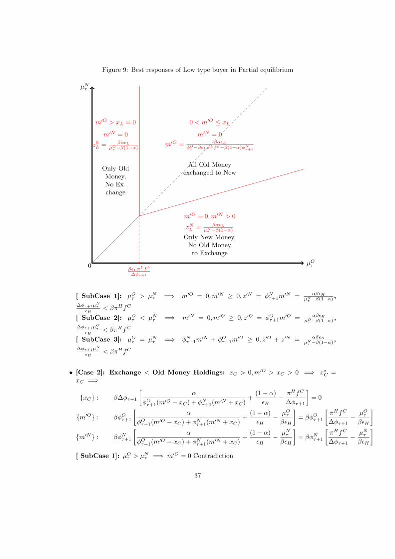
Figure 9: Best responses of Low type buyer in Partial equilibrium
µOτ0
µNτ
βεLπLfL
∆φτ+1
m′O > xL = 0
m′N = 0
Only OldMoney,No Ex-change
z0L = βαεL
µOτ −β(1−α)
0 < m′O ≤ xLm′N = 0
m′O = βαεLφOτ −βεLπLfL−β(1−α)φNτ+1
All Old Moneyexchanged to New
m′O = 0,m′N > 0
zNL = βαεLµNτ −β(1−α)
Only New Money,No Old Moneyto Exchange
[ SubCase 1]: µOτ > µNτ =⇒ m′O = 0,m′N ≥ 0, z′N = φNτ+1m′N = αβεH
µNτ −β(1−α),
∆φτ+1µNτ
εH< βπHfC
[ SubCase 2]: µOτ < µNτ =⇒ m′N = 0,m′O ≥ 0, z′O = φOτ+1m′O = αβεH
µOτ −β(1−α),
∆φτ+1µOτ
εH< βπHfC
[ SubCase 3]: µOτ = µNτ =⇒ φNτ+1m′N + φOτ+1m
′O ≥ 0, z′O + z′N = αβεHµNτ −β(1−α)
,
∆φτ+1µNτ
εH< βπHfC
• [Case 2]: Exchange < Old Money Holdings: xC > 0,m′O > xC > 0 =⇒ x∗C =xC =⇒
{xC} : β∆φτ+1
[α
φOτ+1(m′O − xC) + φNτ+1(m′N + xC)+
(1− α)
εH− πHfC
∆φτ+1
]= 0
{m′O} : βφOτ+1
[α
φOτ+1(m′O − xC) + φNτ+1(m′N + xC)+
(1− α)
εH− µOτβεH
]= βφOτ+1
[πHfC
∆φτ+1− µOτβεH
]{m′N} : βφNτ+1
[α
φOτ+1(m′O − xC) + φNτ+1(m′N + xC)+
(1− α)
εH− µNτβεH
]= βφNτ+1
[πHfC
∆φτ+1− µNτβεH
][ SubCase 1]: µOτ > µNτ =⇒ m′O = 0 Contradiction
37
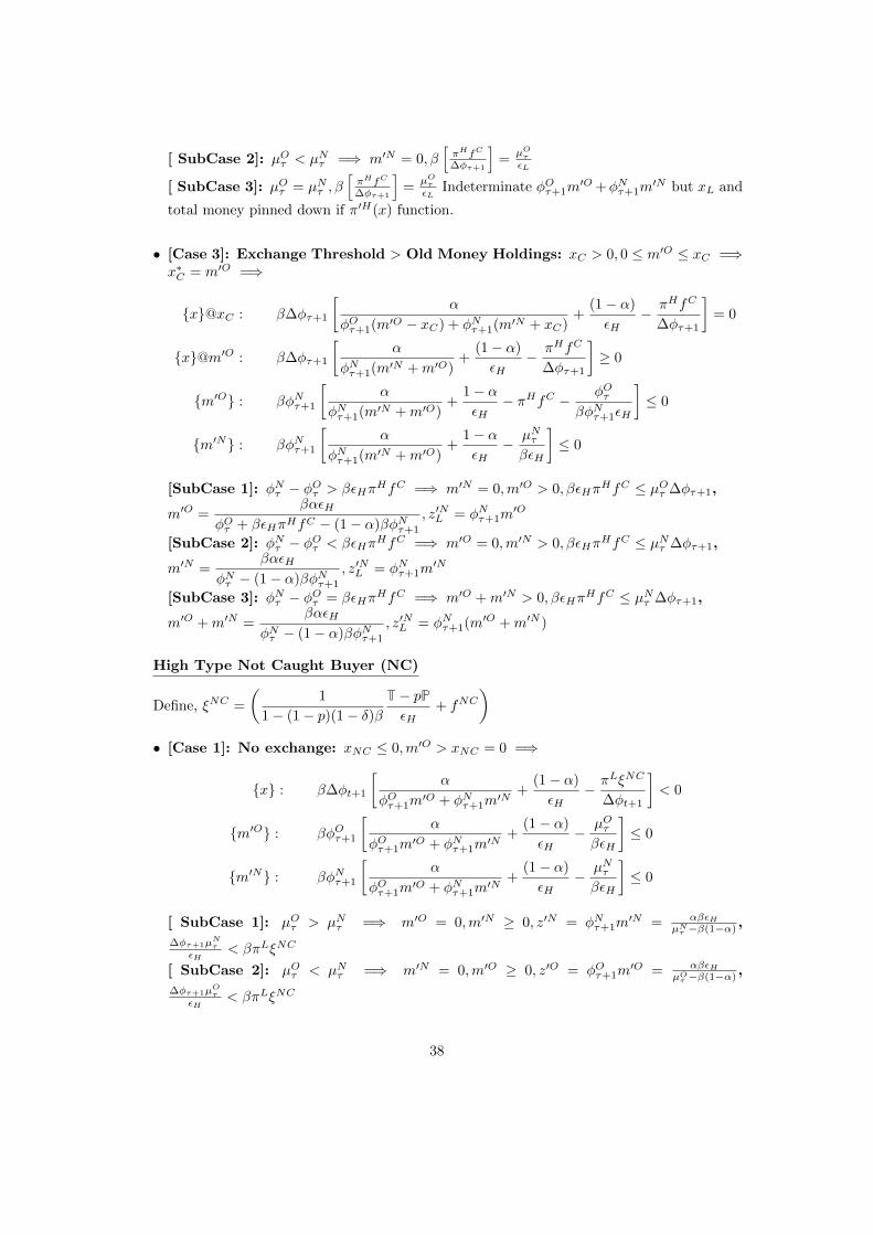
[ SubCase 2]: µOτ < µNτ =⇒ m′N = 0, β[πHfC
∆φτ+1
]=
µOτεL
[ SubCase 3]: µOτ = µNτ , β[πHfC
∆φτ+1
]=
µOτεL
Indeterminate φOτ+1m′O +φNτ+1m
′N but xL and
total money pinned down if π′H(x) function.
• [Case 3]: Exchange Threshold > Old Money Holdings: xC > 0, 0 ≤ m′O ≤ xC =⇒x∗C = m′O =⇒
{x}@xC : β∆φτ+1
[α
φOτ+1(m′O − xC) + φNτ+1(m′N + xC)+
(1− α)
εH− πHfC
∆φτ+1
]= 0
{x}@m′O : β∆φτ+1
[α
φNτ+1(m′N +m′O)+
(1− α)
εH− πHfC
∆φτ+1
]≥ 0
{m′O} : βφNτ+1
[α
φNτ+1(m′N +m′O)+
1− αεH
− πHfC − φOτβφNτ+1εH
]≤ 0
{m′N} : βφNτ+1
[α
φNτ+1(m′N +m′O)+
1− αεH
− µNτβεH
]≤ 0
[SubCase 1]: φNτ − φOτ > βεHπHfC =⇒ m′N = 0,m′O > 0, βεHπ
HfC ≤ µOτ ∆φτ+1,
m′O =βαεH
φOτ + βεHπHfC − (1− α)βφNτ+1
, z′NL = φNτ+1m′O
[SubCase 2]: φNτ − φOτ < βεHπHfC =⇒ m′O = 0,m′N > 0, βεHπ
HfC ≤ µNτ ∆φτ+1,
m′N =βαεH
φNτ − (1− α)βφNτ+1
, z′NL = φNτ+1m′N
[SubCase 3]: φNτ − φOτ = βεHπHfC =⇒ m′O +m′N > 0, βεHπ
HfC ≤ µNτ ∆φτ+1,
m′O +m′N =βαεH
φNτ − (1− α)βφNτ+1
, z′NL = φNτ+1(m′O +m′N )
High Type Not Caught Buyer (NC)
Define, ξNC =
(1
1− (1− p)(1− δ)βT− pPεH
+ fNC)
• [Case 1]: No exchange: xNC ≤ 0,m′O > xNC = 0 =⇒
{x} : β∆φt+1
[α
φOτ+1m′O + φNτ+1m
′N +(1− α)
εH− πLξNC
∆φt+1
]< 0
{m′O} : βφOτ+1
[α
φOτ+1m′O + φNτ+1m
′N +(1− α)
εH− µOτβεH
]≤ 0
{m′N} : βφNτ+1
[α
φOτ+1m′O + φNτ+1m
′N +(1− α)
εH− µNτβεH
]≤ 0
[ SubCase 1]: µOτ > µNτ =⇒ m′O = 0,m′N ≥ 0, z′N = φNτ+1m′N = αβεH
µNτ −β(1−α),
∆φτ+1µNτ
εH< βπLξNC
[ SubCase 2]: µOτ < µNτ =⇒ m′N = 0,m′O ≥ 0, z′O = φOτ+1m′O = αβεH
µOτ −β(1−α),
∆φτ+1µOτ
εH< βπLξNC
38
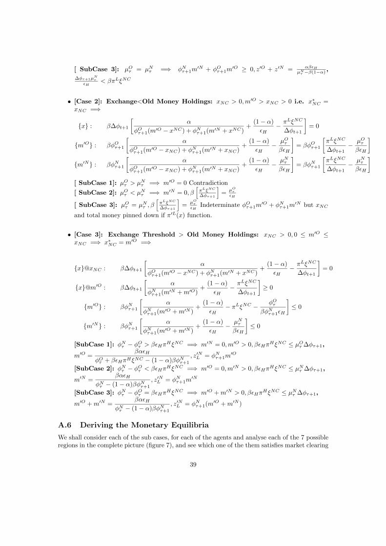
[ SubCase 3]: µOτ = µNτ =⇒ φNτ+1m′N + φOτ+1m
′O ≥ 0, z′O + z′N = αβεHµNτ −β(1−α)
,
∆φτ+1µNτ
εH< βπLξNC
• [Case 2]: Exchange<Old Money Holdings: xNC > 0,m′O > xNC > 0 i.e. x∗NC =xNC =⇒
{x} : β∆φt+1
[α
φOτ+1(m′O − xNC) + φNτ+1(m′N + xNC)+
(1− α)
εH− πLξNC
∆φt+1
]= 0
{m′O} : βφOτ+1
[α
φOτ+1(m′O − xNC) + φNτ+1(m′N + xNC)+
(1− α)
εH− µOτβεH
]= βφOτ+1
[πLξNC
∆φt+1− µOτβεH
]{m′N} : βφNτ+1
[α
φOτ+1(m′O − xNC) + φNτ+1(m′N + xNC)+
(1− α)
εH− µNτβεH
]= βφNτ+1
[πLξNC
∆φt+1− µNτβεH
][ SubCase 1]: µOτ > µNτ =⇒ m′O = 0 Contradiction
[ SubCase 2]: µOτ < µNτ =⇒ m′N = 0, β[πLξNC
∆φτ+1
]=
µOτεH
[ SubCase 3]: µOτ = µNτ , β[πLξNC
∆φτ+1
]=
µOτεH
Indeterminate φOτ+1m′O + φNτ+1m
′N but xNC
and total money pinned down if π′L(x) function.
• [Case 3]: Exchange Threshold > Old Money Holdings: xNC > 0, 0 ≤ m′O ≤xNC =⇒ x∗NC = m′O =⇒
{x}@xNC : β∆φt+1
[α
φOτ+1(m′O − xNC) + φNτ+1(m′N + xNC)+
(1− α)
εH− πLξNC
∆φt+1
]= 0
{x}@m′O : β∆φt+1
[α
φNτ+1(m′N +m′O)+
(1− α)
εH− πLξNC
∆φt+1
]≥ 0
{m′O} : βφNτ+1
[α
φNτ+1(m′O +m′N )+
(1− α)
εH− πLξNC − φOτ
βφNτ+1εH
]≤ 0
{m′N} : βφNτ+1
[α
φNτ+1(m′O +m′N )+
(1− α)
εH− µNτβεH
]≤ 0
[SubCase 1]: φNτ − φOτ > βεHπHξNC =⇒ m′N = 0,m′O > 0, βεHπ
HξNC ≤ µOτ ∆φτ+1,
m′O =βαεH
φOτ + βεHπHξNC − (1− α)βφNτ+1
, z′NL = φNτ+1m′O
[SubCase 2]: φNτ − φOτ < βεHπHξNC =⇒ m′O = 0,m′N > 0, βεHπ
HξNC ≤ µNτ ∆φτ+1,
m′N =βαεH
φNτ − (1− α)βφNτ+1
, z′NL = φNτ+1m′N
[SubCase 3]: φNτ − φOτ = βεHπHξNC =⇒ m′O +m′N > 0, βεHπ
HξNC ≤ µNτ ∆φτ+1,
m′O +m′N =βαεH
φNτ − (1− α)βφNτ+1
, z′NL = φNτ+1(m′O +m′N )
A.6 Deriving the Monetary Equilibria
We shall consider each of the sub cases, for each of the agents and analyse each of the 7 possibleregions in the complete picture (figure 7), and see which one of the them satisfies market clearing
39
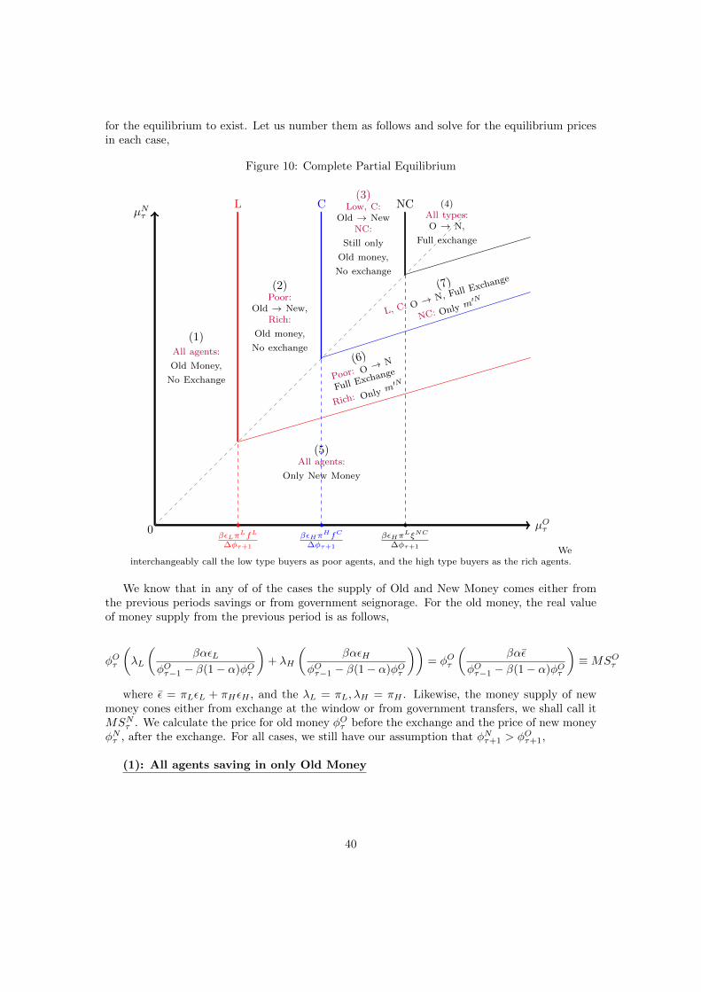
for the equilibrium to exist. Let us number them as follows and solve for the equilibrium pricesin each case,
Figure 10: Complete Partial Equilibrium
µOτ0
µNτL
βεLπLfL
∆φτ+1
C
βεHπHfC
∆φτ+1
NC
βεHπLξNC
∆φτ+1
(1)All agents:
Old Money,
No Exchange
(2)Poor:
Old → New,Rich:
Old money,
No exchange
(3)Low, C:
Old → NewNC:
Still only
Old money,
No exchange
(4)All types:O → N,
Full exchange
(5)All agents:
Only New Money
(6)
Poor: O → N
Full Exchange
Rich: Only m′N
(7)
L, C: O → N, Full Exchange
NC: Only m′N
Weinterchangeably call the low type buyers as poor agents, and the high type buyers as the rich agents.
We know that in any of of the cases the supply of Old and New Money comes either fromthe previous periods savings or from government seignorage. For the old money, the real valueof money supply from the previous period is as follows,
φOτ
(λL
(βαεL
φOτ−1 − β(1− α)φOτ
)+ λH
(βαεH
φOτ−1 − β(1− α)φOτ
))= φOτ
(βαε
φOτ−1 − β(1− α)φOτ
)≡MSOτ
where ε = πLεL + πHεH , and the λL = πL, λH = πH . Likewise, the money supply of newmoney cones either from exchange at the window or from government transfers, we shall call itMSNτ . We calculate the price for old money φOτ before the exchange and the price of new moneyφNτ , after the exchange. For all cases, we still have our assumption that φNτ+1 > φOτ+1,
(1): All agents saving in only Old Money
40
In this case, all the agents have the following demand for real money,
αβε
µOτ − β(1− α)= MDO
τ
Equating this with the money supply, we get that the given equilibrium exists whenever, µOτ <µNτ , and µOt = µ,∀t ≥ τ . For new notes, the only source of supply is government transfers Sτ ,and if we impose that the agents pay their taxes and penalty in terms of new money, we can pindown the new money prices as follows,
φNτ =λCT + λNCpP
Sτ
The prices would be determined for a given level of government transfers. In particular, thegovernment could manipulate and enforce the agents from not staying in this equilibrium bydictating a certain level of inflation using St, but right now, this is an equilibrium. We call itthe ‘Old Money Equilibrium’.
(2): Only poor agents are willing to exchange Old Notes for New
In this case, the agents have the following demand for old money in nominal terms - used forexchange by the poor agents (and hence real value is φNτ+1 ∗ m′O, and for savings to the nextperiod by the rich agents with real value φOτ+1 ∗ m′O, on the LHS and the real money supplyfrom the previous period is as follows
λLβαεL
µOτφOτ+1
φNτ+1− βεLπLfL
φNτ+1− β(1− α)
+ λHβαεH
µOτ − β(1− α)=
βαε
µOτ−1 − β(1− α)
=⇒ µOτ > µOτ−1
Further, we consider the possible cases next period,
1. µNτ+1 > µOτ+1 - in this case, we get that µτ+1+i = µOτ+1 > µOτ > µOτ−1, i.e. the inflation inold money increases as it is scarce in supply when the poor agents exchange it for new, butthen everyone demands only old money next period. In this case the equilibrium breaksdown if the increased inflation in old money surpasses the inflation in new money at anytime.
2. µNτ+1 < µOτ+1 - when old money has higher inflation tomorrow, it is not demanded byanyone, it’s excess supply makes it value less and inflation µOτ actually goes to infinity.This contradicts that the economy is in area 2.
New money prices are determined as in case 1 above. So, the equilibrium either does notexist in region 2, or is extremely fragile to parameters, as any increase in the excess supply ofold money between τ , and τ + 1 can break down the equilibrium. However, this is an interestingequilibrium region because it allows for money laundering and consequent possibility of newmonwy equilibrium as in case (4) below.
(3): Only the Poor agents and Rich honest agents exchange Old Notes for NewThis case is the same as the case 2, except even more fragile. The only possibility of an equi-librium is when the agents continue to hold old money eventually from period τ + 1 onwards,enough such that the inflation in old money is ≤ inflation in new money forever. However if
41

anything like say wear and tear of old notes decreases its money supply, then it’s inflation willincrease and the old money will vanish the moment it’s inflation is greater than that of newmoney. Again, there could be a quick transition to New Money Equilibrium in case the agentscould launder money in period τ.
(4): All agents exchange old money for new - Full Demonetisation
In this case all the agents exchange old money for new, the money market claring conditionin old money is as follows,
λLβαεL
µOτφOτ+1
φNτ+1− βεLπLfL
φNτ+1− β(1− α)
+ λCβαεH
µOτφOτ+1
φNτ+1− βεHπHfC
φNτ+1− β(1− α)
+
λNCβαεH
µOτφOτ+1
φNτ+1− βεHπLξNC
φNτ+1− β(1− α)
=βαε
µOτ−1 − β(1− α)≡MSOτ
and all the new money after exchange which is the new money supply for the next period, isequal to the new money demanded in next period,
λLβαεL
µOτφOτ+1
φNτ+1− βεLπLfL
φNτ+1− β(1− α)
+ λCβαεH
µOτφOτ+1
φNτ+1− βεHπHfC
φNτ+1− β(1− α)
+
λNCβαεH
µOτφOτ+1
φNτ+1− βεHπLξNC
φNτ+1− β(1− α)
=βαε
µNτ+1 − β(1− α)= MDN
τ+1
This puts restrictions on the inflation in new money after transition and inflation in old moneybefore the announcement. Since we are only looking at the stationary equilibrium, we need thatthe new money replaces old money and follows the same path as old money would otherwisehave. The old money completely vanishes from this economy and it is like the φOτ+1 = 0. Isolved for the equilibrium when old money disappears separately, and it appears like the infinitelimit of the x-axis in the complete picture above. i.e. the agents either hold old money andcompletely exchange it for new, when inflation in new money is sufficiently higher than the finethreshold, or they just directly transition to new money and discard all the old money they have(in the absence of laundering) when µNτ , is below the fine threshold. The tilted 45◦, in the partialequilibrium figures, becomes completely horizontal at the threshold values marked on the x- axis.
(5): All agents only hold new money
This is the simplest case of an equilibrium. There is excess supply of Old money, since allthe agents got old money from τ − 1 equal to MSOτ , and no body wants to save in old moneyanymore. This implies that the price of old money goes to 0 immediately and the old moneyseizes to exist. While it may seem that then the equilibrium cannot exist in this area because
µOτ =φOτφOτ+1
, and φOτ ↓ 0, we cannot directly infer this result, because even φOτ+1 = 0. So we move
to the limiting case explained above and all the agents simply hold whatever new money there isin the system with very high price of buying it at τ , and a correspondingly high price of of newmoney tomorrow. So, they are in a high prices high inflation equilibrium for new money, forever(due to stationarity) but the fine in the exchange is sufficiently high for them to want to be in
42

this equilibrium.
MDNτ =
βαε
µNτ − β(1− α)+ λCT + λNCpP = φNτ Sτ = MSNτ
assuming taxes and penalties are to be paid in terms of new money. This is what we shall callthe new money equilibrium. The equilibrium could be made better once all the agents take theone time loss of all their old money in the transition period, if the government decides to givelots of transfers in new money to the agents in the future. But, then the problem of black moneydoes not get mitigated from the system, and none of the agents ever get caught in the exchangewindow imposed by the Demonetisation policy. This equilibrium is the one in which the use ofdemonetisation to curb black money fails miserably.
(6): Honest agents exchange old for new, dishonest agents discard old money
In this equilibrium, all the old money is exchange for new money by the Honest agents (Lowtypes and the High type Caught agents), but the dishonest agents have a huge penalty cost ofkeeping or exchanging old money, so they simply transition to holding new money and discardwhatever old money holdings they had. Again, there is scope for money laundering in this casei.e. the dishonest agents could use their old money and launder if for exchanging to new moneyat a lower cost by giving bribes to the honest agents. In this case, the supply and demand ofnew money is as follows,
MDNτ = λNC
βαεHµNτ − β(1− α)
+ λCT + λNCpP = φNτ Sτ = MSNτ
MSNτ+1 = λLβαεL
µOτφOτ+1
φNτ+1− βεLπLfL
φNτ+1− β(1− α)
+ λCβαεH
µOτφOτ+1
φNτ+1− βεHπHfC
φNτ+1− β(1− α)
+λNCβαεH
µNτ − β(1− α)+ Sτφ
Nτ+1 =
βαε
µNτ+1 − β(1− α)= MDN
τ+1
(7): Poor agents exchange old for new, Rich agents discard old money and save in new
This is the same as the previous case except that the honest agents also choose to take 100%penalty on their old money and directly save in more expensive new money. Again launderingpossibilities will be used by the agents in this case.
43