Black Box Electronics

An Introduction to Applied Electronics for Physicists

5. Pushing the Limits With Spice

University of Toronto

Quantum Optics Group

Alan Stummer, Research Lab TechnologistJune, 2005

2

Spice Programs

• 5 Spice*: Free for non-commercial use with basic version, simple to use, effective, easy to add new models. www.5spice.com

• Linear Technology – LTSpice et al: Free, heavy bias towards Linear Tech’s products, hard to add new models. www.linear.com

• National Semiconductor – WebBench: Free, online only, exclusively National’s components. Limited circuits. www.national.com

• Kemet: Free, exclusively Kemet’s capacitors in frequency domain only but very simple and useful. www.kemet.com

• PSpice: Top price, most features, slightly bloated, need both models and symbols.

* 5 Spice is used in this talk.

3

Common Simulations

• DC Bias: Steady state V and I at t=-0. All capacitors ignored, all inductors shorted. No graphs, tabular results only.

• DC: Same as “DC Bias” except one or more DC sources may be swept through a voltage range.

• AC: Frequency domain. Sweep one or more AC sources through a frequency range.

• Transient: Time domain. Between fixed times. Can also sweep components’ parameter(s).

• Monte Carlo: Time or frequency domain with random selection of any or all component parameters within their specified tolerances. Not available on 5 Spice.

4

Spice Sequence

1. Draw schematic.

2. Select type of simulation.

3. Run simulation.

4. Adjust component values.

5. Repeat with other types of simulation.

5

Adding Components

Move the mouse over the icon to select supplies, click on fixed DC.

6

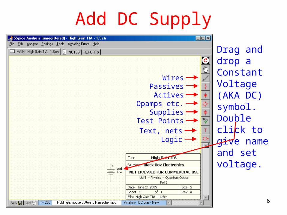
Add DC Supply

Drag and drop a Constant Voltage (AKA DC) symbol. Double click to give name and set voltage.

WiresPassives

ActivesOpamps etc.

SuppliesTest Points

Text, netsLogic

7

Connect Supply

Add ground and supply net, rename net. Right click, move label field to more esthetic location.

8

Add Photodiode Model

Add Current Source and capacitance to simulate a photodiode.

9

Add Generic Opamp

From here…

…add opamp subcircuit symbol. Mirror and rotate for standard orientation.

10

Select LM324

Double click symbol. Set “ref des”, select LM324 model.

This is the model file.

11

Connect Opamp

Add supply and ground. Connect to PD. Add RC feedback.

12

Add Test Point

Monitor this node, call it “Monitor”.

13

DC Bias “Sanity” Check

Select Analysis Dialog (F8), select DC Bias analysis.

Run analysis. Read tabular results or with mouse over node.

14

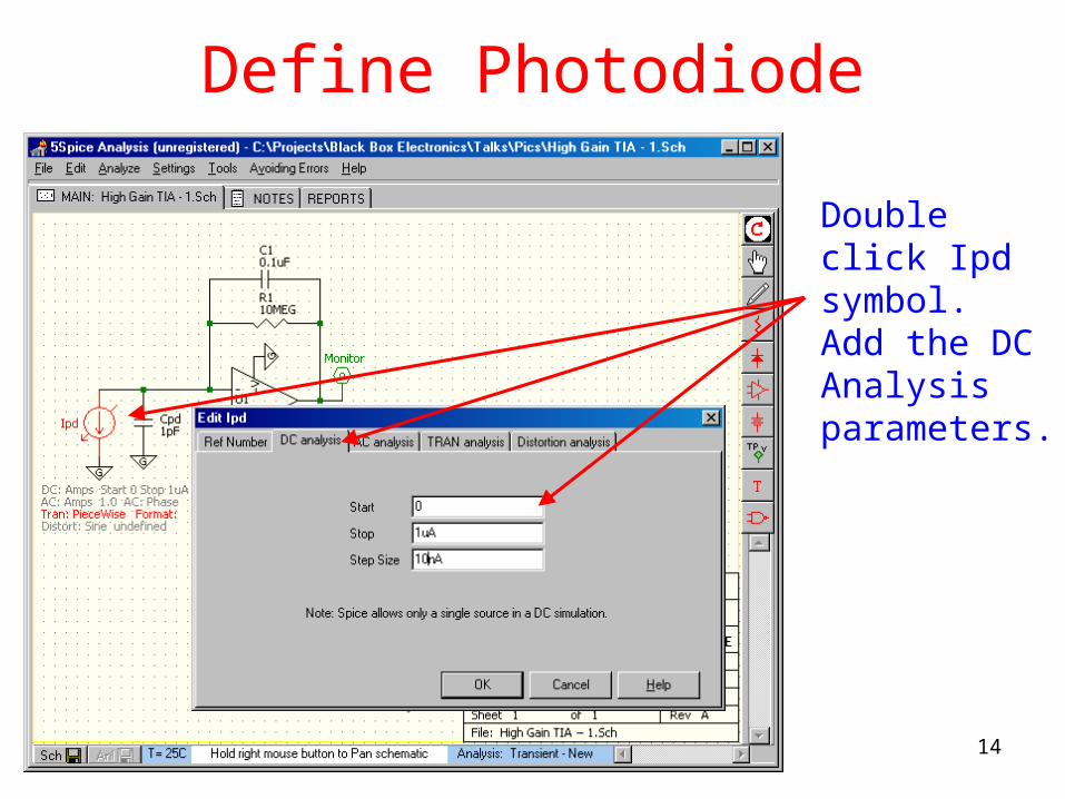
Define Photodiode

Double click Ipd symbol. Add the DC Analysis parameters.

15

Select DC Analysis

Select New Analysis, add DC Analysis, can rename it. Enable Ipd source.

16

Select DC Analysis

On Graph tab, select the Monitor test point and use left axis. Defaults to autoscaling. Hit Enter or Ok and then Run (F9).

17

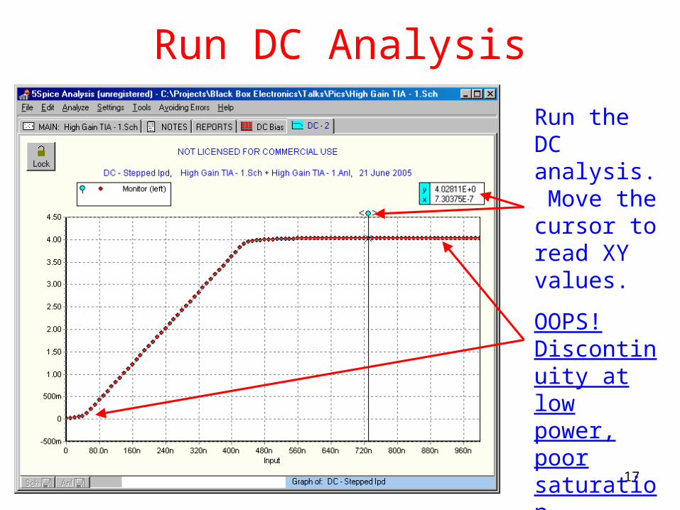
Run DC Analysis

Run the DC analysis. Move the cursor to read XY values.

OOPS! Discontinuity at low power, poor saturation.

18

Try Another Opamp – AD8605

Double click and try another opamp, the AD8605.

19

DC Analysis With AD8605

Note good linearity at low levels and great output saturation.

Keep the AD8605 opamp.

20

Add Second Stage

Copy first stage, paste as second, change ref des on all parts. Rescale Ipd. Second stage voltage gain is +101. Add realistic load.

21

View DC Analysis

Note slight tilt in second stage at low power and output saturation with the added 1KΩ load.

This circuit is acceptable for DC performance!

22

Prepare Transient Analysis

Double click Ipd. Select Transient analysis, Piecewise waveform, define the waveform. Note double 10Sec as 10- and 10+.

23

Transient Analysis

Select Transient analysis. Enable the Ipd source, set start and finish times plus optional step interval time, enable the Helpers, setup the Graph.

24

Run Transient Analysis

Works, but is very very slow, takes 10 seconds to be stable.

Note manual scaling of both Y-axis.

25

Adjust Circuit Timing

Change caps to 100 times smaller, adjust Ipd timing to 100 times faster. Do same to Analysis Dialog, now 0 to 200mS.

26

Final Transient Analysis

Reasonable timing, reasonable gain.

This circuit has been adequately simulated.

27

High Speed Crash

Like before, component values changed for 100 times faster again.

Note step of 1st stage at start, but hidden (damped) by 2nd stage.

Too fast!

28

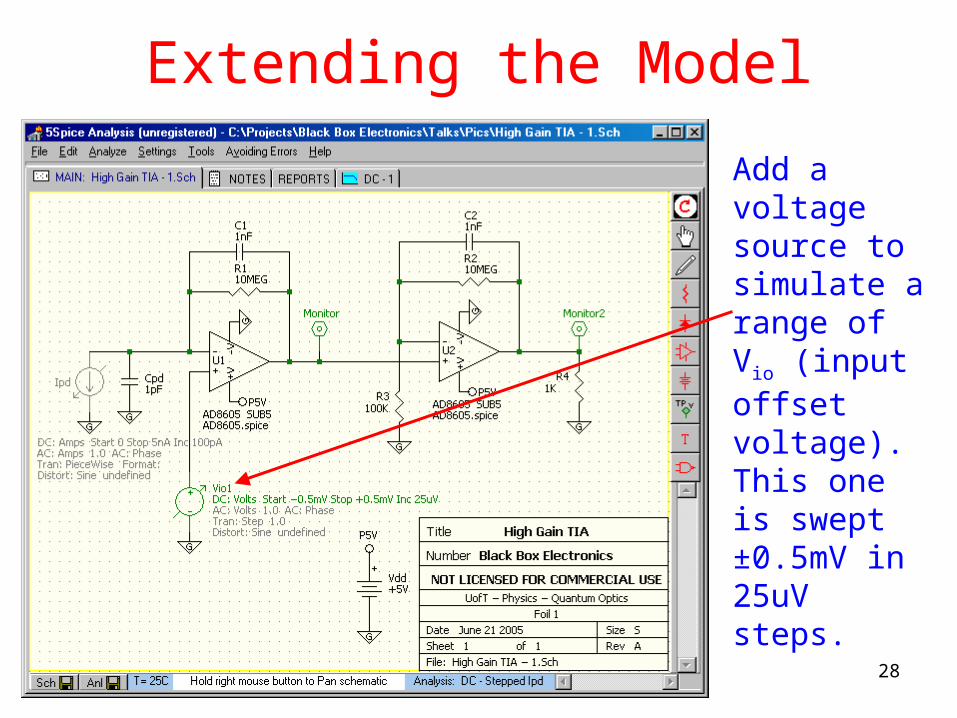
Extending the Model

Add a voltage source to simulate a range of Vio (input offset voltage). This one is swept ±0.5mV in 25uV steps.

29

Extended Model Results

Note how 2nd stage output crosses Y-axis below zero, and how Spice already added some Vio. May want to add an offset to always force above zero or can just ignore.

30

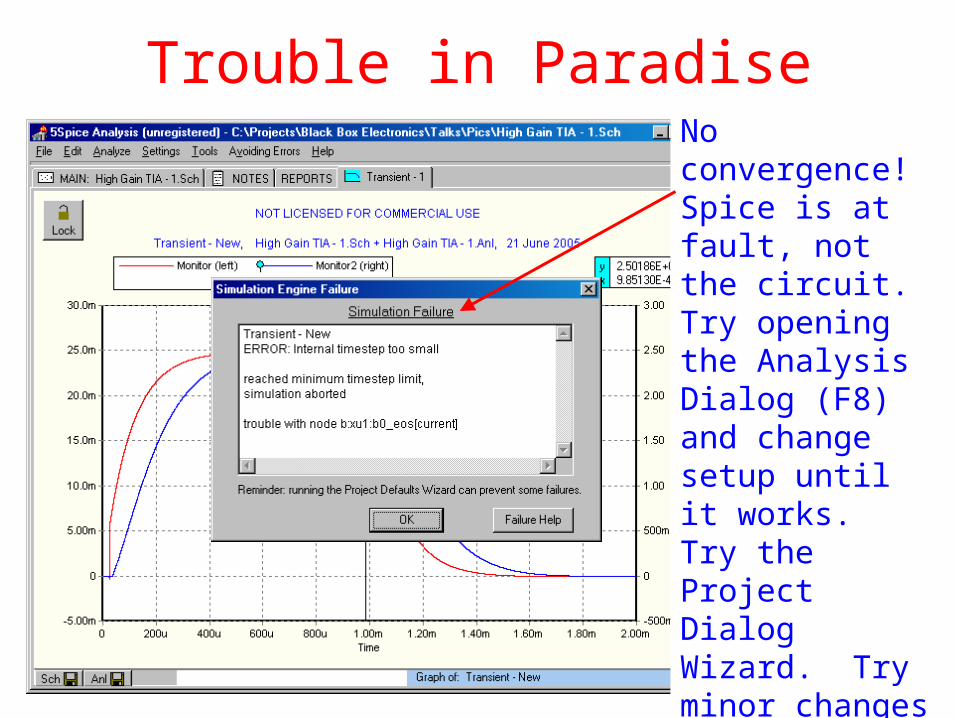
Trouble in ParadiseNo convergence! Spice is at fault, not the circuit. Try opening the Analysis Dialog (F8) and change setup until it works. Try the Project Dialog Wizard. Try minor changes to component values. Good luck!

31

Ω The End Ω

Thanks for coming!

And thanks for the loan of the laptop, Paul!