Bivariate data and cross tabulation

1

Frequency joint distribution

Employee

Director gender

6 M

6 M

10 F

10 F

7 M

3 M

3 M

6 F

4 F

Director gender

M F

3

4

6

7

10

Em

plo

yee

How many shops have 3 employee and a male director? 2

2

How many shops have 3 employee and a female director? 0

0

0

2

1

1

1 0

0 2

2

Frequency joint distribution

Director gender

Tot

M F

3 2 0 2

4 0 1 1

6 2 1 3

7 1 0 1

10 0 2 2

Tot 5 4 9

Em

plo

yee 1 is the joint

distribution corresponding to a shop with 4 employee and a female director

3

Frequency joint distribution

Director gender

Tot

M F

33 22 00 22

44 00 11 11

66 22 11 33

77 11 00 11

1010 00 22 22

Tot 5 4 9

Em

plo

yee

Marginal distribution of director’ gender

Which is the proportion of shop that have a female director?

(44%) 44,094

p

4

Frequency joint distribution

Director gender

Tot

M F

3 22 00 2

4 00 11 1

6 22 11 3

7 11 00 1

10 00 22 2

Tot 55 44 9

Em

plo

yee Marginal distribution of

employee

5

Frequency joint distribution

Director gender

Tot

M F

3 2 00 22

4 0 11 11

6 2 11 33

7 1 00 11

10 0 22 22

Tot 5 44 99

Em

plo

yee

Conditional distribution of the employee for a male director

Which is the mean of the number of employee for shops where the director is a male?

6

Frequency joint distribution

Director gender

Tot

M F

3 22 00 22

4 00 11 11

6 2 1 3

7 11 00 11

10 00 22 22

Tot 55 44 99

Em

plo

yee

Conditional distribution of the director’ gender for shops with 6 employee

If we consider shops with 6 employee, which is the proportion of them with a female director?

7

Frequency joint distributionPlace Shop

on line

city si

suburbs si

Near the city

no

suburbs no

city no

city no

suburbs no

Near the city

no

city si

Shop on line

Tot

si no

city 2 2 4

Near the city

0 2 2

suburbs

1 2 3

Tot 3 6 9P

lace

8

Frequency joint distributionU

bic

azi

on

e

Which is the proportion of shops in the city?

Considering the shops that sell on-line, which is the proportion of shops in the city?

Which is the proportion of shops that sell on-line?

Considering the shops that are in the suburbs, which is the proportion of shops that sell on-line?

9

Shop on line

Tot

si no

city 2 2 4

Near the city

0 2 2

suburbs

1 2 3

Tot 3 6 9

Pla

ce

Frequency joint distributionY Tot

y1 … yj … yK

X

X1 n11 n1j n1k n1.

…

Xi ni1 nij nik ni.

…

xH nH1 nHj nHK nH.

Tot n.1 n.j n.K n

2 marginal distribution

H conditional distribution Y, for each value of X

K conditional distribution X, for each value of Y

10

AssociationThe conditional distributions are the ways of finding out whether there is association between the row and column variables or not. If the row percentages are clearly different in each row, then the conditional distributions of the column variable are varying in each row and we can interpret that there is association between variables, i.e., value of the row variable affects the value of the column variable.

Again completely similarly, if the the column percentages are clearly different in each column, then the conditional distributions of the row variable are varying in each column and we can interpret that there is association between variables, i.e., value of the column variable affects the value of the row variable.

11

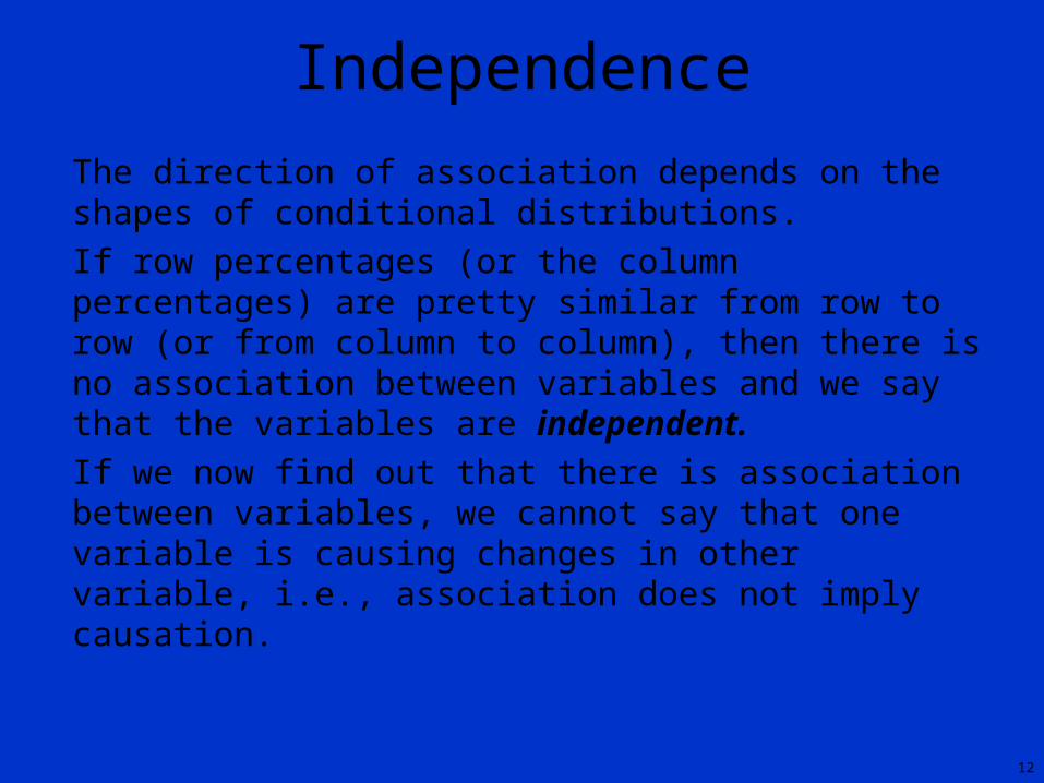
Independence

The direction of association depends on the shapes of conditional distributions.

If row percentages (or the column percentages) are pretty similar from row to row (or from column to column), then there is no association between variables and we say that the variables are independent.

If we now find out that there is association between variables, we cannot say that one variable is causing changes in other variable, i.e., association does not imply causation.

12

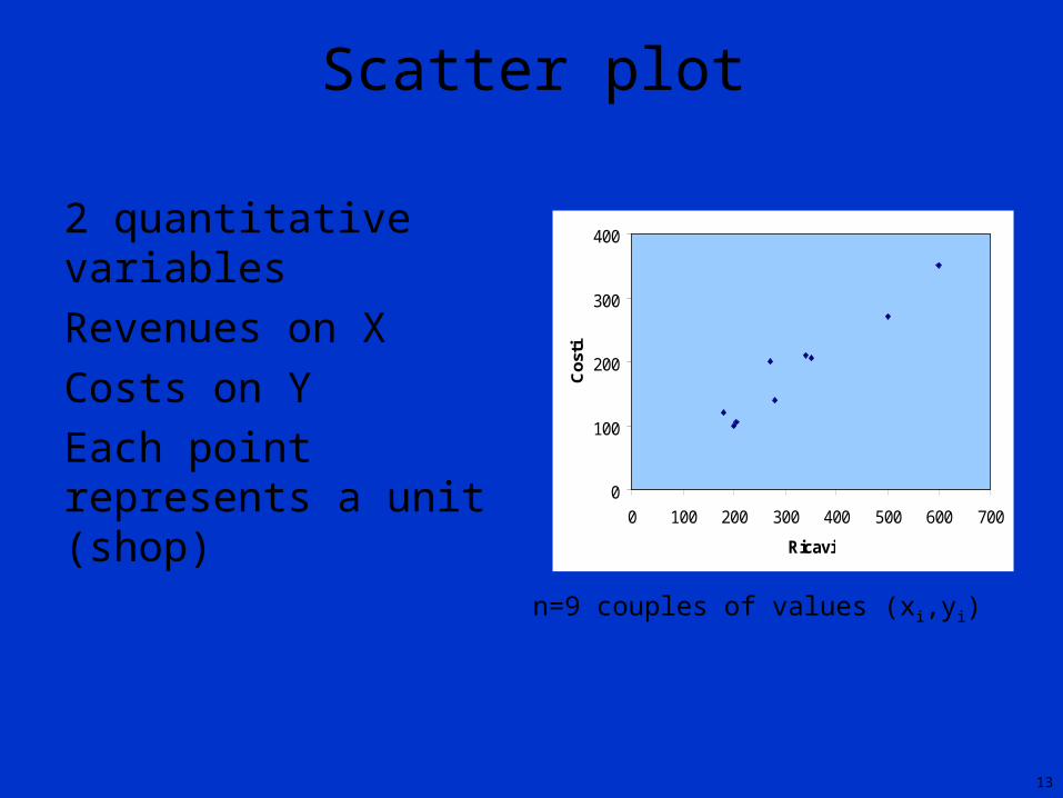
Scatter plot

2 quantitative variablesRevenues on XCosts on YEach point represents a unit (shop) 0

100

200

300

400

0 100 200 300 400 500 600 700

Ricavi

Costi

n=9 couples of values (xi,yi)

13

Grafico di dispersione

We can understand if there is a relation between variablesIn this case…

There is a positive linear realation between revenues and costs.

0

100

200

300

400

0 100 200 300 400 500 600 700

Ricavi

Costi

14

Association between two quantitative variables

Covariance:

Cov > 0 if mostly X and Y move in the same direction.Cov < 0 if mostly X and Y move in opposite directionCov = 0 in absence of any realtion among X and Y

yyxxn1

)Y,X(Cov i

n

1iiXY

15

Cov(X,Y)=0

Null covariance

16

Cov(X,Y)>0

Positive covariance

17

Cov(X,Y)<0

Negative covariance

18

We expect a value of Cov(X,Y) near 0, absence of a linear relationship.

X e Y are NOT independent, but they ave a strong non linear relationship.

Non linear relationship

19

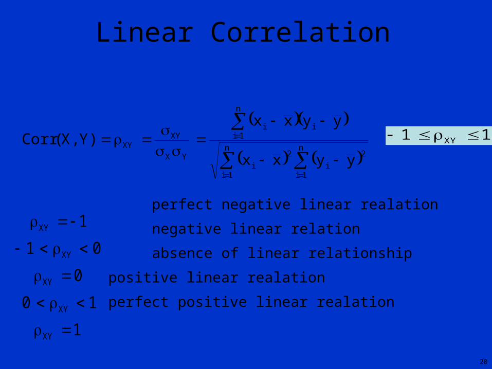
Linear Correlation

perfect negative linear realation

negative linear relation

absence of linear relationship

positive linear realation

perfect positive linear realation

n

1i

2

i

n

1i

2

i

i

n

1ii

YX

XYXY

yyxx

yyxx)Y,X(Corr 11 XY

1XY

01 XY

0XY

10 XY

1XY

20

ρ=1Perfect positive linear relation

ρ=-1Perfect negative linear relation

21

How to calculate covariance(Std. X) x (std. Y)

402,8

11111,1

44305,6

14194,4

-611,1

9988,9

10066,7

316,7

2200,0

Revenue (X)

Costs (Y)

350 205

200 100

600 350

500 270

270 200

180 120

205 105

340 210

280 140

Standard. X

Standard. Y

25 16,11

-125 -88,99

275 161,11

175 81,11

-55 11,11

-145 -68,89

-120 -83,89

15 21,11

-45 -48,89

325 188,89Mean 44,102199

91975)Y,X(Covyyxx

n1

i

n

1ii

22

How to calculate coefficient of correlation

325 188,89

97,048,7866,134

44,10219

YX

XY

Revenue (X)

Costs (Y)

350 205

200 100

600 350

500 270

270 200

180 120

205 105

340 210

280 140

Mean

134,66 78,48Dev std

44,10219)Y,X(Cov

23

We want to invest in the italian stock market and on the one of another country with the aim of diversify our pocket.

Using time siries of the monthly variation of the Morgan Stanley Capital Index (MSCI) for Italy, Germany, France and Singapore we have the following results:

ρ

Italy-France 0.87

Italy-Germany 0.88

Italy-Singapore 0.63

The suggestion is to invest in Italy and Singapore. Why?

24

An application

From the economic theory we know that a relation exists between the variable production (misured with the added value) and the input factors capital and labour. Using the time series (1970-1983) of the 3 variables we have the following scatter plots.

25

Applications

26

The added value has and higher correlation with the input capital (left graph) than with the input labour (right graph).