bischoff auc2008

Advanced Material Modeling in a Virtual Biomechanical Knee

Jeffrey E. Bischoff1, Eik Siggelkow2, Daniel Sieber2, Mariana Kersh3, Heidi Ploeg3, Marc Münchinger2

1Zimmer, Inc., Warsaw, IN

2Zimmer, GmbH, Winterthur, Switzerland

3Department of Mechanical Engineering, University of Wisconsin-Madison, WI

Abstract: For clinicians and medical device manufacturers, in-vitro and in-vivo testing of the knee are important methods for evaluating treatment techniques. However, numerical models that can provide much of the same information will become of more service and are a new focus of the modeling community. A continued effort has centered on specimen-specific anatomical and functional models, in terms of both geometry and mechanical properties of the tissue constituents. Here, a specimen-specific model of the knee is presented that includes the femur, tibia, and four main ligaments (ACL, PCL, MCL, and LCL). Solid models based on CT and MR scans of a human knee joint were meshed in Patran and assembled for solving in Abaqus 6.7-1. Ligaments were modeled using a nonlinear strain energy function which decouples the contributions of the nonlinear, isotropic ground substance (modeled as a neo-Hookean material) and the aligned, nonlinear collagen fibers (modeled using embedded one-dimensional nonlinear springs). Values of the material properties of the ACL were determined using inverse finite element (FE) analysis in which the other three ligaments were resected. Parameter regression was accomplished using the nonlinear local, gradient-based optimization capabilities of both Matlab (Mathworks, Natick, MA) and the optimization software HEEDS (Red Cedar Technology, East Lansing, MI). Analyses for regression assumed a displacement/rotation profile for the femur based on an experimental protocol in development, and optimized against the predicted reaction forces relative to the experimental measurements. Properties of the MCL, LCL, and PCL can be determined sequentially in a similar fashion, thus building up the full knee joint. The ability of the FE model to replicate joint kinematics will be presented, as well as the success of the nonlinear material parameter optimization. Keywords: Biomechanics, Material Optimization, Anisotropic, Soft Tissue, Hyperelasticity

1. Introduction

The knee is the largest and most complex joint within the human body, consisting of both the femoropatellar joint, between the patella and the femur, and the tibiofemoral joint, between the femur and the tibia (Marieb, 2001). Proper motion of the joint relies significantly on the function

2008 Abaqus Users’ Conference 1

of soft tissue constituents including the four ligaments of the tibiofemoral joint: anterior and posterior cruciate ligaments (ACL and PCL, respectively), and medial and lateral collateral ligaments (MCL and LCL, respectively). These ligaments allow primarily flexion/extension and rotation of the joint by enabling the bony constituents (femur and tibia) to translate and rotate relative to each other. In addition to the ligaments, soft cartilage in the joint space permits nearly frictionless contact between the bones. Figure 1 shows a schematic of the tibiofemoral joint including the femur, tibia, fibula, and four ligaments.

Computational modeling of the knee provides a way for better understanding the interplay between the hard and soft tissue constituents of the knee during normal and pathologic function (Li et al, 1999; Donahue et al., 2002). Additionally, properly validated models can be used in the design of knee implant systems by understanding the mechanics of the restored knee including stress and wear of constituent biomaterials (Halloran et al., 2005; Villa et al., 2004; Godest et al., 2002), and guiding optimization of the design in order to more closely replicate the healthy knee.

The overall goal of the work described here is the development of a specimen-specific, validated computational model of the tibiofemoral joint in the human knee. Geometries of the bones and ligaments were derived from CT and MR data and assembled into a computational joint model. Mechanical properties of the constituent ligaments were determined by simulating the response of the model to a rigorous experimental protocol and regressing properties against force/moment versus displacement/rotation data of the experimental model.

This paper is principally concerned with specimen-specific determination of the properties of the ACL, using a realistic constitutive model for the ligament and local optimization techniques. The experimental protocol and overall model framework will initially be described, as both are integral to the parameter estimation process. A fictitious set of experimental data is used here for development of the model and algorithms, which can subsequently be applied to regress parameters against real data. More detail will be devoted to describing and justifying the choice of material models, and detailing the optimization approach and results.

Femur

TibiaFibula

ACL

PCL

LCLMCL

Figure 1. Schematic of the tibiofemoral joint in the human knee.

Femur

TibiaFibula

ACL

PCL

LCLMCL

Figure 1. Schematic of the tibiofemoral joint in the human knee.

2 2008 Abaqus Users’ Conference

2. Methods

The work presented here is one step in constructing a validated specimen-specific finite element (FE) model of the human knee that includes the tibia and femur, as well as the ACL, PCL, MCL, and LCL. Validation of the model will come through an extensive suite of tests on cadaveric knees. In order to establish the numerical approach however, fictitious experimental data were created using specimen-specific geometries of the constituent tissues.

2.1 Experimental Protocol

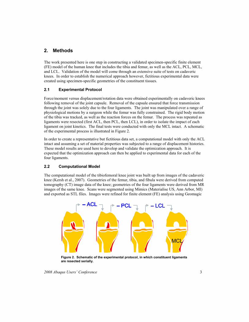
Force/moment versus displacement/rotation data were obtained experimentally on cadaveric knees following removal of the joint capsule. Removal of the capsule ensured that force transmission through the joint was solely due to the four ligaments. The joint was manipulated over a range of physiological motions by a surgeon while the femur was fully constrained. The rigid body motion of the tibia was tracked, as well as the reaction forces on the femur. The process was repeated as ligaments were resected (first ACL, then PCL, then LCL), in order to isolate the impact of each ligament on joint kinetics. The final tests were conducted with only the MCL intact. A schematic of the experimental process is illustrated in Figure 2.

In order to create a representative but fictitious data set, a computational model with only the ACL intact and assuming a set of material properties was subjected to a range of displacement histories. These model results are used here to develop and validate the optimization approach. It is expected that the optimization approach can then be applied to experimental data for each of the four ligaments.

2.2 Computational Model

The computational model of the tibiofemoral knee joint was built up from images of the cadaveric knee (Kersh et al., 2007). Geometries of the femur, tibia, and fibula were derived from computed tomography (CT) image data of the knee; geometries of the four ligaments were derived from MR images of the same knee. Scans were segmented using Mimics (Materialise US, Ann Arbor, MI) and exported as STL files. Images were refined for finite element (FE) analysis using Geomagic

MCL

– ACL – PCL – LCL

Figure 2. Schematic of the experimental protocol, in which constituent ligaments are resected serially.

MCL


MCL


Figure 2. Schematic of the experimental protocol, in which constituent ligaments are resected serially.


(Geomagic, Research Triangle Park, NC). The model was assembled and meshed using Patran (MSC Software, Santa Ana, CA).

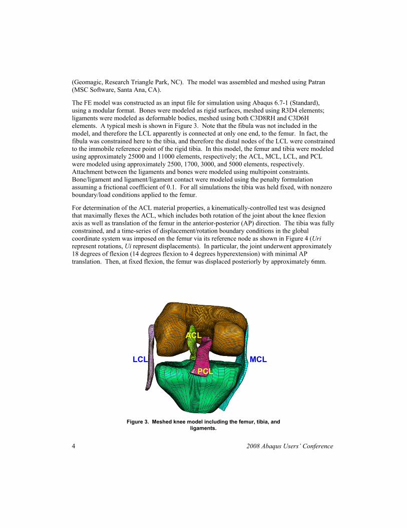
The FE model was constructed as an input file for simulation using Abaqus 6.7-1 (Standard), using a modular format. Bones were modeled as rigid surfaces, meshed using R3D4 elements; ligaments were modeled as deformable bodies, meshed using both C3D8RH and C3D6H elements. A typical mesh is shown in Figure 3. Note that the fibula was not included in the model, and therefore the LCL apparently is connected at only one end, to the femur. In fact, the fibula was constrained here to the tibia, and therefore the distal nodes of the LCL were constrained to the immobile reference point of the rigid tibia. In this model, the femur and tibia were modeled using approximately 25000 and 11000 elements, respectively; the ACL, MCL, LCL, and PCL were modeled using approximately 2500, 1700, 3000, and 5000 elements, respectively. Attachment between the ligaments and bones were modeled using multipoint constraints. Bone/ligament and ligament/ligament contact were modeled using the penalty formulation assuming a frictional coefficient of 0.1. For all simulations the tibia was held fixed, with nonzero boundary/load conditions applied to the femur.

For determination of the ACL material properties, a kinematically-controlled test was designed that maximally flexes the ACL, which includes both rotation of the joint about the knee flexion axis as well as translation of the femur in the anterior-posterior (AP) direction. The tibia was fully constrained, and a time-series of displacement/rotation boundary conditions in the global coordinate system was imposed on the femur via its reference node as shown in Figure 4 (Uri represent rotations, Ui represent displacements). In particular, the joint underwent approximately 18 degrees of flexion (14 degrees flexion to 4 degrees hyperextension) with minimal AP translation. Then, at fixed flexion, the femur was displaced posteriorly by approximately 6mm.

PCL

ACL

MCLLCL

Figure 3. Meshed knee model including the femur, tibia, and ligaments.

PCL

ACL

MCLLCL

Figure 3. Meshed knee model including the femur, tibia, and ligaments.


Figure 4. Boundary conditions imposed on the femur, with the tibia fully constrained, in order to maximally interrogate the properties of the ACL.

(mm)

(rad)

Figure 4. Boundary conditions imposed on the femur, with the tibia fully constrained, in order to maximally interrogate the properties of the ACL.

(mm)

(rad)

2.3 Material Models

Ligaments are composed of highly aligned bundles of collagen fibers, interspersed with cells (fibroblasts) that maintain the extracellular matrix (Woo et al., 2006). Because of this structure, ligaments behave as transversely isotropic materials, with the fiber bundles acting as a single class of fiber reinforcement. Collagen fibers within the bundles are themselves hierarchical in nature, stemming from the base tropocollagen molecule (Fung, 1993). Due to wavy structure within this hierarchy, ligaments can undergo a degree of axial tensile stretch under little load, as the constituents straighten; further load requires distention of the stiff fibers themselves. Thus, the overall response of the ligaments is transversely isotropic and highly nonlinear. Typical ligament response to uniaxial tension along the fiber direction (‘longitudinal’) and transverse to the fiber direction (‘transverse’) is shown in Figure 5, adapted from Quapp and Weiss (1998), illustrating the features of both anisotropy and nonlinearity.

Material modeling of ligaments is normally framed around an additive strain energy function consisting of an isotropic component representing the ground substance of the material and a transversely isotropic component representing the fibrous structure (Holzapfel, 2001). Several such forms have been proposed in the literature (Quapp and Weiss, 1998; Vena et al., 2006), sometimes as the elastic component within the context of more complex viscoelastic material models. Here, the base tissue is modeled using an isotropic (neo-Hookean) strain energy function. Then, several springs are defined that span the ligament between its attachment points. Each spring is assigned nonlinear properties, to reflect the locking behavior seen in ligament tension data. Figure 6 shows the springs within the ACL. In this case, eight springs operated in parallel across the span of the ligament, and eleven springs operated in series over the length of the ligament. End-points of each spring coincided with nodes in the solid model of the ACL, and the spring density was set such that the geometry of the matrix was roughly followed by the springs as deformation occurs.


Figure 5. Typical ligament response to uniaxial tension along the ligament axis ('longitudinal') and transverse to the ligament axis ('transverse').

Figure 5. Typical ligament response to uniaxial tension along the ligament axis ('longitudinal') and transverse to the ligament axis ('transverse').

The force response of each spring is modeled as a three parameter exponential function of displacement

fx ,

( )[ ]{ }1exp 0 −−= xxf βα .

In this model, α correlates with the initial spring stiffness, β affects the degree of nonlinear locking of the spring, and plays the role of ligament prestretch. A set of force versus displacement data is produced based on this relationship and the parameter values; typical implementation is as follows:

0x

Figure 6. Model of the ACL, showing the matrix geometry (left) and the reinforcing, nonlinear springs (right).

Figure 6. Model of the ACL, showing the matrix geometry (left) and the reinforcing, nonlinear springs (right).


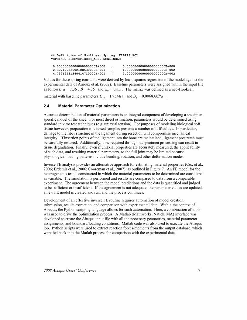
** Definition of Nonlinear Spring: FIBERS_ACL *SPRING, ELSET=FIBERS_ACL, NONLINEAR 0.00000000000000000000E+000 , 0.00000000000000000000E+000 2.30719933692108530000E-001 , 1.00000000000000000000E-002 4.73269131340414710000E-001 , 2.00000000000000000000E-002

Values for these spring constants were derived by least squares regression of the model against the experimental data of Arnoux et al. (2002). Baseline parameters were assigned within the input file as follows: 36.7=α , 35.4=β , and mmx 00 = . The matrix was defined as a neo-Hookean

material with baseline parameters MPaC 95.110 = and . 11 00683.0 −= MPaD

2.4 Material Parameter Optimization

Accurate determination of material parameters is an integral component of developing a specimen-specific model of the knee. For most direct estimation, parameters would be determined using standard in vitro test techniques (e.g. uniaxial tension). For purposes of modeling biological soft tissue however, preparation of excised samples presents a number of difficulties. In particular, damage to the fiber structure in the ligament during resection will compromise mechanical integrity. If insertion points of the ligament into the bone are maintained, ligament prestretch must be carefully restored. Additionally, time required throughout specimen processing can result in tissue degradation. Finally, even if uniaxial properties are accurately measured, the applicability of such data, and resulting material parameters, to the full joint may be limited because physiological loading patterns include bending, rotation, and other deformation modes.

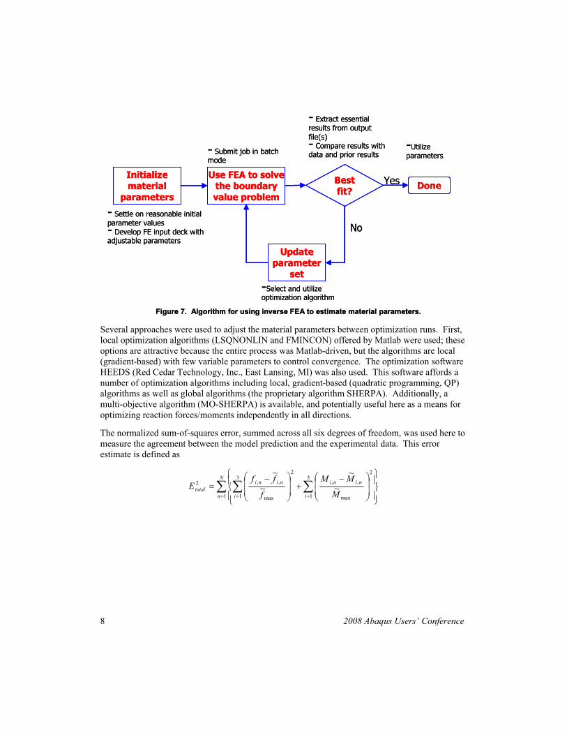
Inverse FE analysis provides an alternative approach for estimating material properties (Cox et al., 2006; Erdemir et al., 2006; Cooreman et al., 2007), as outlined in Figure 7. An FE model for the heterogeneous test is constructed in which the material parameters to be determined are considered as variable. The simulation is performed and results are compared to data from a comparable experiment. The agreement between the model predictions and the data is quantified and judged to be sufficient or insufficient. If the agreement is not adequate, the parameter values are updated, a new FE model is created and run, and the process continues.

Development of an effective inverse FE routine requires automation of model creation, submission, results extraction, and comparison with experimental data. Within the context of Abaqus, the Python scripting language allows for such automation. Here, a combination of tools was used to drive the optimization process. A Matlab (Mathworks, Natick, MA) interface was developed to create the Abaqus input file with all the necessary geometries, material parameter assignments, and boundary/loading conditions. Matlab code was also used to execute the Abaqus job. Python scripts were used to extract reaction forces/moments from the output database, which were fed back into the Matlab process for comparison with the experimental data.


Initialize material

parameters

Use FEA to solve the boundary value problem

Update parameter

set

Best fit? DoneYes

No- Settle on reasonable initial parameter values- Develop FE input deck with adjustable parameters

- Submit job in batch mode

- Extract essential results from output file(s)- Compare results with data and prior results

-Utilize parameters

-Select and utilize optimization algorithm

Figure 7. Algorithm for using inverse FEA to estimate material parameters.

Initialize material

parameters

Use FEA to solve the boundary value problem

Update parameter

set

Best fit? DoneYes

No- Settle on reasonable initial parameter values- Develop FE input deck with adjustable parameters

- Submit job in batch mode

- Extract essential results from output file(s)- Compare results with data and prior results

-Utilize parameters

-Select and utilize optimization algorithm

Figure 7. Algorithm for using inverse FEA to estimate material parameters.

Several approaches were used to adjust the material parameters between optimization runs. First, local optimization algorithms (LSQNONLIN and FMINCON) offered by Matlab were used; these options are attractive because the entire process was Matlab-driven, but the algorithms are local (gradient-based) with few variable parameters to control convergence. The optimization software HEEDS (Red Cedar Technology, Inc., East Lansing, MI) was also used. This software affords a number of optimization algorithms including local, gradient-based (quadratic programming, QP) algorithms as well as global algorithms (the proprietary algorithm SHERPA). Additionally, a multi-objective algorithm (MO-SHERPA) is available, and potentially useful here as a means for optimizing reaction forces/moments independently in all directions.

The normalized sum-of-squares error, summed across all six degrees of freedom, was used here to measure the agreement between the model prediction and the experimental data. This error estimate is defined as

∑ ∑∑= == ⎪⎭

⎪⎬⎫

⎪⎩

⎪⎨⎧

⎟⎟

⎠

⎞

⎜⎜

⎝

⎛ −+

⎟⎟

⎠

⎞

⎜⎜

⎝

⎛ −=

N

n i

nini

i

ninitotal M

MM

f

ffE

1

3

1

2

max

,,3

1

2

max

,,2~

~

~

~


where and represent the model reaction force and moment, respectively, in direction i

at time point n , nif , niM ,

nif ,~

and niM ,~ represent the corresponding experimental values, and

( )nif ,f max~~

max= and ( )niMM ,max~max~

= represent the maximum experimental force and moment across all directions and data points. Note that this error metric therefore does not differentiate between force and moment or between directions.

Prior to optimization, a sensitivity analysis was performed using the spring-reinforced material model. In particular, each of the five material parameters of the ACL were varied in the vicinity of their respective baseline values, and the overall response on model error was calculated. Those parameters which most significantly impacted the model error were optimized, whereas those with minimal effect were held constant during the optimization process.

3. Results

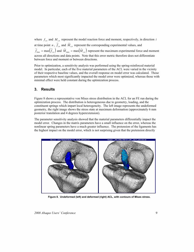
Figure 8 shows a representative von Mises stress distribution in the ACL for an FE run during the optimization process. The distribution is heterogeneous due to geometry, loading, and the constituent springs which impart local heterogeneity. The left image represents the undeformed geometry, the right image shows the stress state at maximum deformation (approximately 6 mm posterior translation and 4 degrees hyperextension).

The parameter sensitivity analysis showed that the material parameters differentially impact the model error. Changes in the matrix parameters have a small influence on the error, whereas the nonlinear spring parameters have a much greater influence. The pretension of the ligaments has the highest impact on the model error, which is not surprising given that the pretension directly

Figure 8. Undeformed (left) and deformed (right) ACL, with contours of Mises stress.


impacts the locking stretch of the springs. However, it was also noted during the sensitivity analysis that varying pretension can impact overall model convergence. Thus, for purposes here the spring parameters α and β and the matrix parameter are optimized. 10C

In comparison to the Matlab local optimization toolbox, the HEEDS optimization software provided a much friendlier optimization environment through its graphical user interface. The effort to implement a comparable user interface in Matlab would be considerable. More importantly, the convergence behavior of the HEEDS quadratic programming algorithm was more stable than the Matlab algorithms. Therefore, the remainder of this study focuses on optimization results using HEEDS.

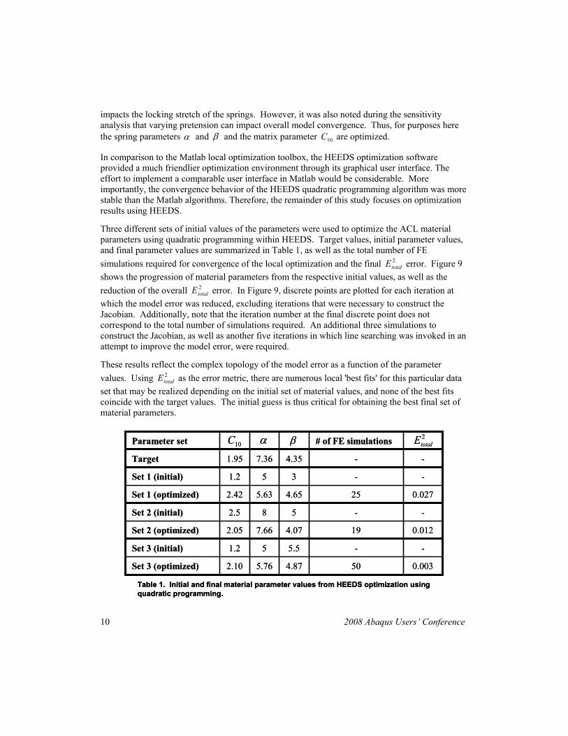
Three different sets of initial values of the parameters were used to optimize the ACL material parameters using quadratic programming within HEEDS. Target values, initial parameter values, and final parameter values are summarized in Table 1, as well as the total number of FE simulations required for convergence of the local optimization and the final error. Figure 9 shows the progression of material parameters from the respective initial values, as well as the reduction of the overall error. In Figure 9, discrete points are plotted for each iteration at which the model error was reduced, excluding iterations that were necessary to construct the Jacobian. Additionally, note that the iteration number at the final discrete point does not correspond to the total number of simulations required. An additional three simulations to construct the Jacobian, as well as another five iterations in which line searching was invoked in an attempt to improve the model error, were required.

2totalE

2totalE

These results reflect the complex topology of the model error as a function of the parameter values. Using as the error metric, there are numerous local 'best fits' for this particular data set that may be realized depending on the initial set of material values, and none of the best fits coincide with the target values. The initial guess is thus critical for obtaining the best final set of material parameters.

2totalE

Table 1. Initial and final material parameter values from HEEDS optimization using quadratic programming.

10C α β 2totalE

0.003504.875.762.10Set 3 (optimized)

--5.551.2Set 3 (initial)

0.012194.077.662.05Set 2 (optimized)

--582.5Set 2 (initial)

0.027254.655.632.42Set 1 (optimized)


--4.357.361.95Target

# of FE simulationsParameter set

Table 1. Initial and final material parameter values from HEEDS optimization using quadratic programming.

10C α β 2totalE

0.003504.875.762.10Set 3 (optimized)

--5.551.2Set 3 (initial)

0.012194.077.662.05Set 2 (optimized)


0.027254.655.632.42Set 1 (optimized)


--4.357.361.95Target

# of FE simulationsParameter set


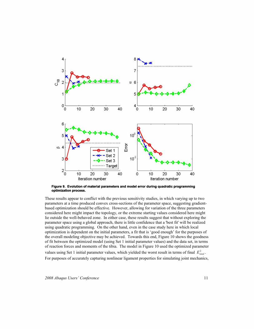
Figure 9. Evolution of material parameters and model error during quadratic programming optimization process.Figure 9. Evolution of material parameters and model error during quadratic programming optimization process.

These results appear to conflict with the previous sensitivity studies, in which varying up to two parameters at a time produced convex cross-sections of the parameter space, suggesting gradient-based optimization should be effective. However, allowing for variation of the three parameters considered here might impact the topology, or the extreme starting values considered here might lie outside the well-behaved zone. In either case, these results suggest that without exploring the parameter space using a global approach, there is little confidence that a 'best fit' will be realized using quadratic programming. On the other hand, even in the case study here in which local optimization is dependent on the initial parameters, a fit that is ‘good enough’ for the purposes of the overall modeling objective may be achieved. Towards this end, Figure 10 shows the goodness of fit between the optimized model (using Set 1 initial parameter values) and the data set, in terms of reaction forces and moments of the tibia. The model in Figure 10 used the optimized parameter values using Set 1 initial parameter values, which yielded the worst result in terms of final . For purposes of accurately capturing nonlinear ligament properties for simulating joint mechanics,

2totalE


Figure 10. Model predictions of tibia reaction force and moment (lines) in comparison to target values (symbols). Forces and moments using the initial set of parameters are plotted using dashed lines; final values are plotted using solid lines, and are nearly coincident with the target values.

Figure 10. Model predictions of tibia reaction force and moment (lines) in comparison to target values (symbols). Forces and moments using the initial set of parameters are plotted using dashed lines; final values are plotted using solid lines, and are nearly coincident with the target values.

and taking into account limitations on the accuracy of the experimental data (including degradation of tissue during the testing process), the goodness of fit is more than sufficient.

4. Discussion

The work presented here is a preliminary study on the use of optimization techniques for material parameter estimation within a computational model of the knee. There are several ongoing areas of study that will expand the utility of the computational model, as follows.

4.1 Ligaments

Optimization of the mechanical properties of the ACL is one step in developing a specimen-specific model of the knee. Inclusion of the other ligaments (PCL, MCL, and LCL), and estimation of the properties of these ligaments based on experiments designed to interrogate their responses, is also required. A similar process as has been outlined here can be used on these ligaments.

4.2 Material Model

The work presented here exclusively used an isotropic hyperelastic continuum model (neo-Hookean) for the ACL, reinforced by several discrete one-dimensional springs. This model is computationally more expensive than an isotropic model, but presumably is more capable in capturing experimental data. On the other hand, this formulation may not be as accurate as anisotropic hyperelastic continuum models that have been developed and validated in the literature for capturing ligament material data (Holzapfel, 2001; Quapp and Weiss, 1998). Accordingly, a


transversely isotropic, nonlinear hyperelastic model has been developed as a user material based on the strain energy function

( )[ ]{ }11exp2

242

2

1 −−+=+= IkkkWWWW NHTINH

This model is a continuum strain energy function appropriate for a material with one family of reinforcing fibers (Holzapfel, 2001), and is based on decoupling the strain energy function into an isotropic (neo-Hookean) component denoted and a transversely isotropic component,

denoted . The anisotropic strain invariant NHW

TIW 4I is defined as ( )CA :4 trI = where is

the material orientation tensor associated with the locally defined fiber orientation ,

aaA ⋅= T

a CC 32−= J is the modified right Cauchy-Green tensor, and and C are the Jacobian and the right Cauchy-Green tensor, respectively.

J

This material model has been incorporated into Abaqus using a UMAT user subroutine. At each integration point, the initial coordinate location is used to identify the fiber orientation, which is mapped to be roughly parallel to the ligament edge throughout the domain. This orientation, along with the material properties and the deformation gradient, are the only required inputs to the subroutine. Components of the Cauchy stress tensor are calculated directly from the strain energy function. Components of the material Jacobian are calculated numerically, using an algorithm similar to that of Mao (2006), whereby the logarithmic strains are perturbed slightly and the effect on the Cauchy stress tensor is evaluated.

Use of this model, in place of the spring-reinforced model used to generate the results presented here, has the advantage of requiring a fewer number of material parameters, and thus the optimization process should proceed more quickly. On the other hand, there is likely still coupling between the stiffness of the neo-Hookean strain energy function ( ) and that of the reinforcing fibers ( ), which can compromise the uniqueness of the parameter set unless the base data are supplemented with data reflecting the transverse material response. Future work will explore these issues.

10C

1k

4.3 Error Calculation

The error calculation used to generate the results here is , as defined previously. While this error estimate reflects average model fit across the entire deformation and all degrees of freedom, it will not reflect potentially large deviations between model prediction and experiment that may occur over short durations, or only at particular flexion angles. Additionally, does not discriminate between moments and forces. Other metrics can thus be defined if average goodness of fit is not sufficient. For example, the maximum normalized error between the model and the data could be used. This error is more sensitive to large errors that may be realized over a short

2totalE

2totalE


duration along a single axis, whereas is more concerned with the average response across all directions and all time points.

2totalE

4.4 Optimization Algorithm

All results used here follow from use of local optimization techniques. However, it has been shown that within the context of this particular data set, use of different initial sets of parameters will affect the optimization results. Use of global techniques is thus warranted, in order to remove the need for a good first guess of material parameters and to have greater confidence that the final set of material parameters is in fact optimized across the parameter space. To achieve this, the proprietary algorithm SHERPA offered within HEEDS can be used, which is a hybrid approach combining local and global features. Additionally, a multi-objective algorithm (MO-SHERPA) is available, and could be used here as a means for optimizing reaction forces/moments independently in all directions. In particular, the error estimate could be resolved into components along each of the six axes, in order to more fully understand the origin of disagreement between model and data, and then to make intelligent optimization decisions that best suit the purposes of the computational model.

2totalE

5. Conclusions

A finite element model of the human knee has been developed that uses specimen-specific geometry and material properties. An inverse FE routine for regressing values of ligament material parameters against trial data sets has been used to contrast various optimization strategies, emphasizing the need for experimental data that fully encapsulates the material response. Uniqueness of this procedure is compromised by coupling between material parameters, which can potentially be addressed by employing alternative error metrics or material models. This approach will assist in developing specimen-specific computational models for use in orthopaedic implant design.

6. References

1. Arnoux, P.J., P. Chabrand, M. Jean, and J. Bonoit, “A Visco-hyperelastic Model With Damage for the Knee Ligaments Under Dynamic Constraints”, Computer Methods in Biomechanics and Biomedical Engineering, 5 (2), 167-174, 2002.

2. Cooreman, S., D. Lecompte, H. Sol, J. Vantomme, and D. Debruyne, “Elasto-plastic material parameter identification by inverse methods: Calculation of the sensitivity matrix”, International Journal of Solids and Structures, 44, 4329-4341, 2007.

3. Cox, M.A.J., N.J.B. Driessen, C.V.C. Bouten, and F.P.T. Baaijens, “Mechanical Characterization of Anisotropic Planar Biological Soft Tissues Using Large Indentation: A Computationl Feasilbitty Study”, Journal of Biomechanical Engineering, 128, 428-436, 2006.


4. Donahue, T.L.H., M.L. Hull, M.M. Rashid, and C.R. Jacobs, “A Finite Element Model of the Human Knee Joint for the Study of Tibio-Femoral Contact”, Journal of Biomechanical Engineering, 124, 273-280, 2002.

5. Erdemir, A., M.L. Viveiros, J.S. Ulbrecht, P.R. Cavanagh, “An inverse finite-element model of heel-pad indentation”, Journal of Biomechanics, 39, 1279-1286, 2006.

6. Fung, Y.C., “Biomechanics: Mechanical Properties of Living Tissues”, Second Edition, Springer-Verlag, New York, 1993.

7. Godest, A.C., M. Beaugonin, E. Haug, M. Taylor, and P.J. Gregson, “Simulation of a knee joint replacement during a gait cycle using explicit finite element analysis”, Journal of Biomechanics, 35, 267-275, 2002.

8. Halloran, J. P., A. J. Petrella, and P. J. Rullkoetter, “Explicit finite element modeling of total knee replacement mechanics”, Journal of Biomechanics, 38, 323-331, 2005.

9. Holzapfel, G. A., “Nonlinear Solid Mechanics: A Continuum Approach for Engineering”, John Wiley & Sons, Ltd., England, 2001.

10. Kersh, M.E., H. Ploeg, R. Burgkart, E. Siggelkow, and M. Münchinger, “Creating a physiological knee model: experimental methods and validation concept”, International Society of Biomechanics Conference, Taipei, Taiwan, 2007.

11. Li, G., J. Gil, A. Kanamori, and S. L.-Y. Woo, “A Validated Three-Dimensional Computational Model of a Human Knee Joint”, Journal of Biomechanical Engineering, 121, 657-662, 1999.

12. Mao, K., “An Effective Numerical Approach in Implementing the Consistent Jacobian Matrix in Material Model Developments Using User Subroutine UMAT in ABAQUS”, 2006 ABAQUS Users’ Conference, West Lafayette, IN, 2006.

13. Marieb, E.N., “Human Anatomy & Physiology”, Fifth Edition, Pearson Education, Inc., San Francisco, 2001.

14. Quapp, K. M. and J. A. Weiss, “Material Characterization of Human Medial Collateral Ligament”, Journal of Biomechanical Engineering, 120, 757-763, 1998.

15. Vena, P., D. Gastaldi, and R. Contro, “A Constituent-Based Model for the Nonlinear Viscoelastic Behavior of Ligaments”, Journal of Biomechanical Engineering, 128, 449-457, 2006.

16. Villa, T., F. Migliavacca, D. Gastaldi, M. Colombo, and R. Pietrabissa, “Contact stresses and fatigue life in a knee prosthesis: comparison between in vitro measurements and computational simulations”, Journal of Biomechanics, 37, 45-53, 2004.

17. Woo, S. L.-Y., S. D. Abramowitch, R. Kilger, and R. Liang, “Biomechanics of knee ligaments: injury, healing, and repair”, Journal of Biomechanics 39, 1-20, 2006.


bischoff auc2008

Documents