birmingham city health and economic impact assessment … executive summary and key results uk100...

Birmingham City Health and Economic Impact Assessment study

For: UK:100

By: David Dajnak, Heather Walton and James David Smith

Final Report

Address: Environmental Research Group, School of Analytical, Environmental and Forensic Sciences , King’s College London, Franklin-Wilkins Building, 150 Stamford Street, London, SE1 9NH, United Kingdom. Tel: +44 207 848 4009, email: [email protected]

Web: https://www.kcl.ac.uk/lsm/research/divisions/aes/research/ERG/index.aspx

London monitoring: http://www.londonair.org.uk/LondonAir/Default.aspx

https://www.kcl.ac.uk/lsm/research/divisions/aes/research/ERG/index.aspx

http://www.londonair.org.uk/LondonAir/Default.aspx

Table of Contents 1.0 Executive Summary and Key results 3

2.0 Introduction 6

3.0 Method 6

3.1 Air Quality data 6

3.2 Health assessment 6

3.3 Economic assessment 7

4.0 Air Quality modelling 9

5.0 Health Estimates of the mortality impact of air pollution and its economic valuation 12

5.1 Mortality impact 12

5.2 Life-expectancy from birth in 2011 17

6.0 Health Estimates of the mortality burden of air pollution 19

6.1 Burden background 19

6.2 Combined estimate for PM2.5 and NO2 using multi pollutant model results 19

6.3 Single pollutant model estimates 21

6.4 Summary of burden results 22

7.0 Discussion 23

8.0 Appendix 26

8.1 Additional tables- method 26

8.2 Additional tables - impact 28

8.3 Additional tables – burden 37

8.4 Additional Health and economic assessment methods 41

9.0 References 45

1.0 Executive Summary and Key results

UK100 commissioned Kings College London (King’s) to produce a health and economic impact assessment associated with current1 and future pollution levels in Birmingham City. In this study, King’s combined the relationships between Defra’s Air Quality modelling concentrations and health outcomes for each parliamentary constituency in Birmingham. King’s has previously carried out similar mortality burden calculations for London and Greater Manchester but to our knowledge this is the first time that the new burden recommendations (COMEAP, 2018a)2 that include a combined PM2.5 and NO2 approach have been applied in practice in a large city area3. The calculations relate to deaths or loss of life expectancy from all causes rather than separately for specific causes or for cases of specific illnesses. Mortality impact (long –term exposure) The population in Birmingham would gain around 440,000 life years over a lifetime to 21344 if air pollution concentrations improved as projected from 2011 to 20305, compared with remaining at 2011 concentrations. The average life expectancy of a child born in Birmingham in 2011 would improve by around 2.5 to 4 months for the same comparison. Taking into account the UK Government’s projected future changes in air pollution concentrations from 2011 to 2030, the population would still be losing between 0.3 to 0.8 million life years after these air pollution changes in Birmingham (a life year is one person living for one year). Put another way, children born in 2011 are still estimated to die 2-7 months early6 on average, if exposed over their lifetimes to the projected future air pollution concentrations in Birmingham. Males are more affected than females. This is due to the fact that men have higher death rates and die earlier than women The report provides figures for both PM2.5 and NO2 separately but then uses one or the other as the best indicator pollutant rather than adding results together to avoid large overestimation (details in the report below). The ‘best indicator’ approach may result in a small underestimate. Economic costs

1 Birmingham air quality annual status report (2018) shows that Birmingham has been in breach of both the national air quality objective for NO2 and the World Health Organization guideline for PM2.5. https://www.birmingham.gov.uk/downloads/file/11938/air_quality_annual_status_report_2018_containing_data_for_2017 2 COMEAP – the Committee on the Medical Effects of Air Pollutants is a national expert Committee advising Government on the health effects of air pollution. Their recommendations for quantification are usually used in Government cost-benefit analysis of policies to reduce air pollution. 3 Mortality burden calculations for the UK, England, Wales, Scotland and Northern Ireland can be found in the COMEAP (2018) report itself. 4 It is not possible to calculate the full result for gains in life expectancy until everyone in the initial population has died (105 years from 2030), necessitating follow-up for a life-time even if the pollution changes are only for the next decade or so. 5 2011 and 2015 concentrations representing current reference years and any future years up to 2030 have been estimated from the 2015 baseline. Note that the government data projections to 2030 were produced before the Birmingham Clean Air Zone was proposed 6 The range is according to whether indicator pollutant is taken as PM2.5 or NO2, whether or not there is a cut-off concentration below which no effects are assumed and gender (Table 4 in report).

https://www.birmingham.gov.uk/downloads/file/11938/air_quality_annual_status_report_2018_containing_data_for_2017


Economists assign monetary values to the health benefits in order to compare the benefits with the real costs of implementing a package of policies. The largest proportion of the monetary value comes from a survey asking 170 members of the public how much they would be willing to pay to reduce their risk of experiencing a loss of one month of life (in good health) due to air pollution. Added up across time, people and the total health effects, this is then used to represent the amount society thinks should be spent to reduce these risks. NHS costs and loss of productivity are not included. The monetized benefits over a lifetime7 of improvements to future anthropogenic PM2.5 and NO2 concentrations, compared with 2011 concentrations remaining unchanged, has been estimated to be up to £240 million on average/year (at 2014 prices). Despite the projected future improvements in air pollution concentrations from 2011 to 2030, the economic health impact costs in Birmingham over a lifetime are still between £190 - £470 million on average per year. These are what is called ‘annualised’ figures - a term for an average per year when the result is not the same every year. They are not actual costs but a measure of the amount of money society believes it would be reasonable to spend on policies to reduce air pollution (for avoiding adverse health effects of the remaining pollution) or was reasonable to have spent on policies that have already reduced air pollution. Mortality burden (long –term exposure) Mortality burden calculations are a simplified calculation at one point in time. They are not suitable for analyzing several years in succession because they do not have a mechanism for allowing the number of deaths the year before to influence the age and population size the following year (lifetables do this, see impact calculations above). Nonetheless, they provide a useful feel for the size of the air pollution problem. In 2011 in Birmingham the equivalent of8 between 570 to 709 deaths are estimated to be attributable to air pollution (anthropogenic PM2.5 and NO2). These deaths occur mostly at older ages, as is typical for deaths in the general population. The results varied by constituency with highest in Erdington and lowest in Hall Green. The ranking by constituency did not fully follow the ranking in pollutant concentrations. This is because the results are also influenced by variations in death rates by constituency, which in turn are driven in part by the proportion of elderly in the population and the level of deprivation. The results for both life years lost after pollution improvements and attributable deaths from 2011 are smaller than the results for Greater Manchester from a 2018 report, primarily due to the smaller population in the smaller area of Birmingham city (around 1 million compared with 2.7 million for Greater Manchester). But they are not as much smaller as the population would predict due to higher pollution concentrations in Birmingham City. This also shows in the fact that the loss of life

7 From 2030, so the total time period was 2011-2134. 8 The original studies were analysed in terms of ‘time to death’ aggregated across the population. Strictly, it is unknown whether this total change in life years was from a smaller number of deaths fully attributable to air pollution or a larger number of deaths to which air pollution partially contributed. The former is used with the phrase ‘equivalent’ to address this issue. See COMEAP (2010) for a fuller discussion.

expectancy (which is independent of population) is greater in Birmingham than in Manchester. Gains in life years are smaller in Birmingham City than in Greater Manchester, again mainly due to population and the similar proportional reduction in pollution concentrations over time. Limitations The main report presents a wider range of uncertainty around the results for the mortality burden, mortality impacts and economic costs than the figures shown here. The study was focused on air pollution changes within the Birmingham city area. Reductions in emissions will also have benefits for air pollution concentrations in the wider region (the West Midlands and beyond). For example, reductions in NOx emissions will reduce nitrate concentrations and thus PM2.5 concentrations in the wider region. The health benefits of this are not reflected here, although they are likely to be smaller than those in the city itself. There will be further impacts from ozone concentrations. The long-term ozone exposure (representative of summer smog ozone concentrations metric) is projected to decrease over time compared with 2011 but less than other pollutants such as NO2 and PM2.5. This study addressed the effect of air pollution on deaths and loss of life-expectancy. This included all causes of death grouped together so covers, for example, respiratory, lung cancer and cardiovascular deaths for which there is good evidence for an effect of air pollution. It does not, however, cover the effect of air pollution on health where this does not result in death. So well established effects (such as respiratory and cardiovascular hospital admissions, effects on asthma, low birth weight etc) and other outcomes more recently potentially linked with air pollution (such as dementia) are not included. Their inclusion would increase the benefit of policies to further reduce air pollution.

2.0 Introduction

UK100 has asked King’s College London (King’s) to help produce an Health Impact assessment (HIA) and economic assessment of Birmingham City (Birmingham) formed of ten parliamentary constituencies (constituencies) (Edgbaston, Erdington, Hall Green, Hodge Hill, Ladywood, Northfield, Perry Barr, Selly Oak, Yardley and Sutton Coldfield). To do this, King’s first downloaded the air quality data in Birmingham, which then, combined with relationships between concentrations and health outcomes, were used to calculate the impacts on health from the air pollution emitted in each constituency.

3.0 Method

3.1 Air Quality data

From 1kmx1km grid data to ward concentration To create maps of annual average air quality (PM2.5 and NO2) for Birmingham, King’s downloaded air quality data from the DEFRA Local Air Quality Management webpages (https://uk-

air.defra.gov.uk/data/laqm-background-maps). Specifically, we downloaded PM2.5 and NO2 data for the regions of 'Midlands' for the year 2011, and for the years 2015 to 2030. The 2011 data were downloaded from the 2011 model predictions, and the 2015 to 2030 data were downloaded from the 2015 model predictions. Using these data of regular 1km by 1km pollutant points we then created a raster layer (for every year and pollutant) in the R statistical analysis package. Mean spatially-weighted concentrations for each Ward were then calculated, using the Ward boundaries from the Governments Open Data portal (http://geoportal.statistics.gov.uk/datasets/wards-december-

2016-generalised-clipped-boundaries-in-the-uk). From ward to population-weighted constituency concentration Population-weighting average concentration (PWAC): Population-weighting was done at Ward level. The ward concentrations were multiplied by the population aged 30 plus for each gender and the resulting population-concentration product summed across all wards in each constituency and then divided by the constituency population. The constituency population-weighted means were then used directly in the health impact calculations across all constituencies. (This process allows one health calculation per constituency rather than calculations in each separate ward). A map of Birmingham parliamentary constituencies can be found in Figure 1.

3.2 Health assessment

It is now well established that adverse health effects, including mortality, are statistically associated with outdoor ambient concentrations of air pollutants. Moreover, toxicological studies of potential mechanisms of damage have added to the evidence such that many organisations (e.g. US Environmental Protection Agency; World Health Organisation, COMEAP) consider the evidence strong enough to infer a causal relationship between the adverse health effects and the air pollution concentrations. The concentration-response functions used and the spatial scales of the input data is given in Table 10, Table 11 and Table 12 in the Appendix. The concentration-response functions are based on

https://uk-air.defra.gov.uk/data/laqm-background-maps

https://uk-air.defra.gov.uk/data/laqm-background-maps

http://geoportal.statistics.gov.uk/datasets/wards-december-2016-generalised-clipped-boundaries-in-the-uk

http://geoportal.statistics.gov.uk/datasets/wards-december-2016-generalised-clipped-boundaries-in-the-uk

the latest advice from the Committee on the Medical Effects of Air Pollutants in 2018 (COMEAP, 2018a). Previously, burden calculations were based only on concentrations of PM2.5 (COMEAP, 2010). The new COMEAP report considers whether there is an additional burden or impact from nitrogen dioxide or other pollutants with which it is closely correlated. Results are given with and without a cut-off9 of 5 µg m-3 for NO2 and 7 µg m-3 for PM2.5. This study uses this epidemiological evidence to estimate the health impacts of the changes in air pollutant concentrations discussed in the air quality modelling section below.

3.3 Economic assessment

Economists assign monetary values to the health benefits in order to compare the benefits with the real costs of implementing a package of policies. The largest proportion of the monetary value comes from a survey asking 170 members of the public how much they would be willing to pay to reduce their risk of experiencing a loss of one month of life (in good health) due to air pollution (Chilton et al, 2004). Added up across time, people and the total health effects, this is then used to represent the amount society thinks should be spent to reduce these risks. NHS costs and loss of productivity are not included. In undertaking a valuation in monetary terms of the mortality impacts described in the previous section, we have used the methods set out in an earlier report from King’s College London on the health impacts of air pollution in London (Walton et al., 2015) and in King’s latest NIHR report (Williams et al., 2018b). This built on previous work by the study team for Defra and the Inter-departmental Group on Costs and Benefits (IGCB) within the UK government. The methods are therefore consistent with those used in government in the UK. Life years lost were valued using values recommended in Defra guidance10, updated to 2014 prices. Consistent with this guidance, values for future life years lost were increased at 2% per annum, then discounted using the declining discount rate scheme in the HMT Green Book.11 The economic impact was then annualised back to 2014, i.e. divided by the total number of years but front-loaded to take into account that benefits accrued sooner are valued more than those accrued later.

9 Cut-off is a term used for the concentration below which it is unclear whether or not epidemiological evidence supports the existence of an effect. This does not mean there is no effect below the cut-off, just that the numbers of data points are too small to be sure one way or the other. 10 Defra (2019) Impact Pathways Approach Guidance for Air Quality Appraisal 11 HM Treasury (2018) The Green Book

Figure 1 Map of Birmingham’s parliamentary constituencies12

12 https://www.birmingham.gov.uk/downloads/file/4604/map_birmingham_constituencies

https://www.birmingham.gov.uk/downloads/file/4604/map_birmingham_constituencies

4.0 Air Quality modelling

2011 and 2015 concentrations representing current reference years and any future years up to 2030 have been estimated from the 2015 baseline13. Birmingham air quality annual status report (2018) shows that Birmingham has been in breach of both the national air quality objective for NO2 and the World Health Organization guideline for PM2.5 (https://www.birmingham.gov.uk/downloads/file/11938/air_quality_annual_status_report_2018_containing_data_fo

r_2017). The reader should refer to the Background Maps User guide (https://laqm.defra.gov.uk/review-

and-assessment/tools/background-maps.html#about) for information on an estimated breakdown of the relative source of pollution and on how pollutant concentrations change over time. A summary of the population-weighted average concentration (PWAC) between 2011 and 2030 in each constituency is shown in Table 1 and Table 2 for anthropogenic PM2.5 and NO2, respectively. Table 1 Anthropogenic PM2.5 PWAC (in μg m-3) (annual) by constituency

Local authority 2011 2015 2020 2025 2030

Edgbaston 12.21 9.35 8.79 8.61 8.56

Erdington 13.58 10.38 9.75 9.55 9.52

Hall Green 12.57 9.61 9.02 8.83 8.79

Hodge Hill 13.41 10.11 9.49 9.31 9.27

Ladywood 14.24 11.02 10.29 10.10 10.08

Northfield 11.60 8.96 8.43 8.25 8.21

Perry Barr 13.58 10.52 9.88 9.69 9.67

Selly Oak 12.00 9.15 8.60 8.42 8.38

Yardley 12.91 9.73 9.13 8.95 8.91

Sutton Coldfield 12.08 9.24 8.70 8.52 8.48

Table 2 NO2 PWAC (in μg m-3) (annual) by constituency

Local authority 2011 2015 2020 2025 2030

Edgbaston 23.34 18.69 15.46 12.66 11.14

Erdington 29.66 23.89 19.67 16.22 14.35

Hall Green 24.87 20.88 17.33 14.49 12.92

Hodge Hill 28.63 23.99 20.04 16.98 15.26

Ladywood 32.54 28.03 23.29 19.60 17.54

Northfield 20.89 16.38 13.59 11.24 9.95

Perry Barr 29.55 23.45 19.11 15.75 13.95

Selly Oak 22.62 18.19 15.16 12.69 11.35

Yardley 26.42 22.00 18.46 15.76 14.21

Sutton Coldfield 22.63 17.82 14.72 12.14 10.71

Maps of PM2.5 and NO2 annual mean concentration by wards are shown in Figure 2 and Figure 3, respectively.

13 Note that the government data projections to 2030 were produced before the Birmingham Clean Air Zone was proposed



https://laqm.defra.gov.uk/review-and-assessment/tools/background-maps.html#about

https://laqm.defra.gov.uk/review-and-assessment/tools/background-maps.html#about

Figure 2 Annual mean PM2.5 concentrations (in μg m-3) by wards between 2011 and 2030

City Centre

Figure 3 Annual mean NO2 concentrations (in μg m-3) by wards between 2011 and 2030

City Centre

5.0 Health Estimates of the mortality impact of air pollution and its

economic valuation

5.1 Mortality impact

Impacts in the next section are all expressed in terms of life years – the most appropriate metric for the health impact of air pollution concentration changes over time. This used a full life-table approach rather than the short-cut method used for burden and the data for these calculations had already been incorporated for previous work (Williams et al., 2018a). Calculations are first given for PM2.5 and NO2 separately. Because air pollutants are correlated with each other, the air pollutant concentrations in the health studies represent both the pollutants themselves but also other air pollutants closely correlated with them. Health impacts from changes in NO2 and PM2.5 represent the health impacts of changes in the air pollution mixture in slightly different ways that overlap i.e. they should not be added. This is discussed further at the end of this section. The results from the life table calculations assuming that the concentration does not reduce from 2011 levels and assuming the predicted concentration between 2011 and 2030 (concentrations were modelled at 2011, 2015, 2020, 2025 and 2030 but also interpolated for the intervening years) are shown in Table 3, for anthropogenic PM2.5 and NO2. Results for each constituency can be found in the Appendix in Table 13 and Table 17 (life table calculations for anthropogenic PM2.5 with and without a cut-off), in Table 14 and Table 18 (life table calculations for NO2 with and without a cut-off) and Table 15 and Table 16 (central and lower/upper CI estimates of annualised economic impact for anthropogenic PM2.5 and NO2 without a cut-off) and Table 19 (central CI estimates of annualised economic impact for anthropogenic PM2.5 and NO2 with a cut-off ). The life years lost gives a large number because the life years (one person living for one year) is summed over the whole population in Birmingham over 124 years. For context, the total life years lived with baseline mortality rates is around 198 million, so these losses of life years involve about 0.5% of total life years lived. If 2011 concentrations of anthropogenic PM2.5 remained unchanged for 124 years, around 0.6 – 1.2 million life years would be lost across Birmingham’s population over that period. This improves to around 0.2 – 0.8 million life years lost with the predicted concentration between 2011 and 2030 changes examined here. Another way of representing the health impacts if air pollution concentrations remained unchanged (in 2011) compared with the projected future changes (2011 to 2030) is provided by the results for NO2. If 2011 concentrations of NO2 remained unchanged for 124 years, around 0.8 – 0.9 million life years would be lost across Birmingham’s population over that period. This improves to around 0.3 – 0.5 million life years lost with the predicted concentration between 2011 and 2030 changes examined here. Summarising these results is not easy. The results should not be added as there is considerable overlap. On the other hand, either result is an underestimate to some extent as it is missing the impacts that are better picked up in the calculations using the other pollutant. COMEAP (2017,

2018a) suggested taking the larger of the two alternatives in the calculation of benefits. We have interpreted this as the larger of the two alternatives in the case of each calculation. Note that this means that the indicator pollutant changes in different circumstances. In the case above, for no cut-off, this is the result for PM2.5 (0.8 vs 0.5 million life years lost for NO2). However, for the cut-off, this is the result for NO2 (0.3 vs 0.2 million life years lost for PM2.5). This is one of the first times these recommendations have been applied in practice, so other interpretations e.g. keeping the same indicator pollutant with and without a cut-off, are possible. All the relevant data are in the tables to enable creation of summaries in a different form. So, the overall summary for the projected future changes in air pollution concentrations from 2011 to 2030 would be around 0.3 to 0.8 million life years lost for the population of Birmingham over 124 years. Table 3 Total life years lost across the Birmingham population for anthropogenic PM2.5 and NO2

and the associated annualised economic impact (central estimate)

Pollutant

Scenario

Life years lost

Central estimate

(without cut-off

with cut-off)

Annualised economic

impact (in 2014 prices)

(without cut-off

with cut-off)

Anthropogenic PM2.5 (representing

the regional air pollution mixture

and some of the local mixture)

Concentration does not

reduce from 2011 levels

1,169,520

562,960

£653,424,492

£313,958,210

Predicted concentration

between 2011 and 2030

831,708

213,344

£467,766,599

£121,993,163

NO2 (representing the local

mixture and the rural air pollution

mixture)



942,827

767,457

£525,828,421

£427,680,084



505,434

328,491

£289,339,663

£190,370,755

For anthropogenic PM2.5 assuming no net migration, with projected new births, 2011-2134, compared with life years lived with baseline mortality rates (incorporating mortality improvements over time) with a relative risk (RR) of 1.06 per

10 μg m-3 of anthropogenic PM2.5 without cut-off and with 7 μg m-3 cut-off14, with lags from the USEPA.

For NO2 assuming no net migration, with projected new births, 2011-2134, compared with life years lived with baseline mortality rates (incorporating mortality improvements over time) with a relative risk (RR) of 1.023 per 10 μg m-3 of NO2 without cut-off and with 5 μg m-3 cut-off, with lags from the USEPA. (Results with cut-offs do not extrapolate beyond the original data, results with no cut-off represent the possibility that there are effects below the cut-off value (it is unknown whether or not this is the case).) Figures in bold are the larger of the alternative estimates using PM2.5 or NO2, as summarized in the headline results.

Table 3 also gives the economic impacts (economic costs). Note that these are derived from applying monetary valuation to the health impacts. The monetary values are derived from surveys

14 It is possible that this cut-off will be defined at a value lower than 7 μg m-3 in the future as this is based on a 2002 study. The concentration-response function and its confidence intervals have been updated using a 2013 meta-analysis (the central estimate happened to remain the same). The cut-off has not so far been updated to reflect the range of the data in the meta-analysis.

of what people are willing to pay to avoid the risk of the relevant health impact. They do not represent the costs of the policies or the costs to the NHS. If 2011 concentrations of anthropogenic PM2.5 remained unchanged for 124 years, the annualised economic cost would be around £310 – 650 million. This improves to around £120 – 470 million with the projected baseline concentration changes examined here. If 2011 concentrations of NO2 remained unchanged for 124 years, the annualised economic cost would be around £430 – 530 million. This improves to around £190 – 290 million with the predicted concentration between 2011 and 2030 changes examined here. The overall summary for the projected baseline would be annualised economic costs of around £190 to 470 million.

Figure 4 Cumulative life years lost for anthropogenic PM2.5 and NO2 if 2011 concentrations

remained unchanged and the baseline (current policies 2011-2030) across the Birmingham

population (no migration), with projected new births, compared with life years lived with baseline

mortality rates (incorporating mortality improvements over time) 2011-2134. RR 1.06 per 10 μg m-

3 for anthropogenic PM2.5 and RR 1.023 per 10 μg m-3 for NO2, EPA lag

* Cut-off results not shown

Figure 4 shows that the cumulative life years lost for the predicted concentration between 2011 and

2030 accumulates more slowly than the constant 2011 concentration results for both anthropogenic PM2.5 and NO2 as a result of the reduced concentrations from 2011 to 2030. It is worth remembering that there is a delay before the full benefits of concentration reductions are achieved. This is not just due to a lag between exposure and effect, but also because the greatest gains occur when mortality rates are highest i.e. in the elderly. Table 4 shows the differences between the predicted concentrations between 2011 and 2030 and both particulate levels and NO2 concentration constant at 2011 levels. Using PM2.5 as an indicator of the regional pollution and some of the local pollution mixture gives an estimate of 340,000 to 350,000 life years gained as a result of the predicted concentration between 2011 and 2030. Using NO2 as an indicator of mostly the local pollution mixture and the rural pollution gives a larger estimate of 440,000 life years gained. This makes sense because the concentration projected (2011 to 2030) suggests more continuous declines in NO2 concentrations (likely to be mostly due to the improvement in NOX emissions of large parts of the road transport sector) than for PM2.5, reflecting the fact that PM reduction from traffic is not larger due to the increasing contribution from non-exhaust emissions and also that the declines in regional PM2.5 are relatively small. Thus, using NO2 rather than PM2.5, as the indicator of changes in the traffic pollution mixture seems more appropriate for future changes as presented here. This is a different indicator compared with the overall impact in terms of life years lost15. Regional pollution is a greater contributor to absolute total concentrations than to future changes so there is also some sense in PM2.5 being the indicator in this case. The overall summary would be that taking into account predicted air pollution concentration changes

between 2011 and 2030, the population in Birmingham would gain around 440,000 life years over a lifetime.

15 This was not the case for the cut-off, where NO2 rather than PM2.5 gives the larger result. But this may be mostly to do with the value of the cut-off.

Table 4 Life years saved (and associated monetised benefits) across Birmingham population of the

predicted concentration between 2011 and 2030 compared with 2011 anthropogenic PM2.5

concentrations and NO2 remaining unchanged

Pollutant Scenario

Total life years saved

compared with 2011

concentrations maintained

(without cut-off

with cut-off)

Monetised benefits

compared with 2011

concentrations maintained

(without cut-off

with cut-off)

Anthropogenic PM2.5

(representing the regional

air pollution mixture and

some of the local mixture)

Predicted

concentration

between 2011

and 2030

337,812 349,616

£185,657,893 £191,965,047

NO2 (representing the local

mixture and the rural air

pollution mixture)

Predicted

concentration

between 2011

and 2030

437,393 438,966

£236,488,758 £237,309,329

Figures in bold are the larger of the alternative estimates using PM2.5 or NO2, as summarized in the headline results.

Table 4 also provides an estimate of the economic impact as a result of the improvements in pollution from 2011 to 2030 versus 2011 pollution remaining unchanged. The annualised monetary benefit of anthropogenic PM2.5 and NO2 improvements has been estimated to be up to £240 million (at 2014 prices).

Figure 5 Life years gained per year from long-term exposure to the improvements in pollution

from 2011 to 2030 of anthropogenic PM2.5 and NO2 relative to 2011 concentrations remaining

unchanged

* Cut-off results not shown

Figure 5 shows the effect of the decrease in PM2.5 and NO2 concentration from 2011 to 2030 (as seen in Table 1 and Table 2).

5.2 Life-expectancy from birth in 2011

Total life years across the population is the most appropriate metric for cost-benefit analysis of policies as it captures effects in the entire population. However, it is a difficult type of metric to communicate as it is difficult to judge what is a ‘small’ answer or a ‘large’ answer. Life-expectancy from birth is a more familiar concept for the general public, although it only captures effects on those born on a particular date. Results for life expectancy from birth are shown in Table 5. Results for each constituency can be found in the Appendix in Table 20 and Table 21 (Loss of life expectancy for anthropogenic PM2.5 and NO2 with and without a cut-off). This shows that the average loss of life expectancy from birth in Birmingham would be about 20 – 41 weeks for male and 17 – 35 weeks for female if 2011 PM2.5 concentrations were unchanged but improves to 7 – 29 weeks for male and 6 – 25 weeks for female for the predicted concentration between 2011 and 2030 (an improvement by about 10-13 weeks). Using NO2, the average loss of life expectancy from birth in Birmingham would be about 27 – 33 weeks for male and 23 – 28 weeks for female if NO2 concentrations were unchanged from 2011 but

improves by about 13-16 weeks to 11 – 17 weeks for male and 9 – 15 weeks for female with projected future changes between 2011 and 2030 included. The overall summary would be that the projected future changes provide an improvement in average life expectancy from birth in 2011 of around 2.5 – 4 months (11 – 17 weeks) but an average loss of life expectancy from birth in 2011 of around 2 to 7 months (9 – 29 weeks) remains even with the reduced concentrations. Males are more affected than females – this is mainly due to the higher mortality rates in men compared with women rather than differences in air pollution exposure. Table 5 Loss of life expectancy by gender across Birmingham from birth in 2011 (followed for 105

years) for anthropogenic PM2.5 and NO2

Pollutant

Scenario

Loss of life expectancy from birth compared with

baseline mortality rates, 2011 birth cohort (in weeks)

(without cut-off

with cut-off)

Male Female

Anthropogenic

PM2.5



40.9

19.8

34.9

17.0



28.8

7.2

24.6

6.2

NO2



33.2

27.1

28.4

23.2



17.0

10.9

14.5

9.3

Figures in bold are the larger of the alternative estimates using PM2.5 or NO2, as summarized in the headline results.

Additional data such as the loss of life expectancy lower and upper estimate and the full range of confidence intervals with and without the counterfactual for both PM2.5 and NO2 are available upon request to the authors.

6.0 Health Estimates of the mortality burden of air pollution

6.1 Burden background

Burden calculations are a snapshot of the burden in one year, assuming that concentrations had been the same for many years beforehand. They are intended as a simpler calculation than the more detailed assessments that are given above (in the mortality impact section). They are not suitable for calculation is several successive years as they do not have a mechanism for allowing the number of deaths the year before to influence the age and population size the following year as the lifetables used in impact calculations do. They are included here as a comparison with similar calculations presented elsewhere (COMEAP, 2010; Walton et al., 2015; Dajnak et al., 2018). The concentration-response functions used for these calculations are evolving over time. Previous recommendations favoured methods similar to the single pollutant model approach presented below. The latest COMEAP (2018a) report shows that a majority of the committee supported a new approach using information from multi pollutant model results but COMEAP (2018a) also recommended using a range to reflect the uncertainty. Single pollutant models relate health effects to just one pollutant at a time, although because pollutants tend to vary together, they may in fact represent the effects of more than one pollutant. Single pollutant models for different pollutants cannot therefore be added together as there may be substantial overlap. Multi-pollutant models aim to disentangle the effects of separate pollutants but this is difficult to do. Despite the best attempts, it may still be the case that some of the effect of one pollutant ‘attaches’ to the effects ascribed to another pollutant, leading to an underestimation of the effects of one pollutant and an overestimation of the effects of another. In this situation, the combined effect across the two pollutants should give a more reliable answer16 than the answers for the individual pollutants that may be over- or under-estimated. This was the basis for the approach described below, including adding results derived from information within each of 4 separate studies first, before combining them as a range. The intention is not to present the individual pollutant results separately as final results, although the calculations are done as intermediate stages towards the overall results. [Burden calculations would normally include accompanying estimates of the burden life years lost17. This would require inputting average loss of life expectancy by age and gender for calculations in each ward. For this small project, it was not possible to do this.] The calculations are based on deaths from all causes including respiratory, lung cancer and cardiovascular deaths, the outcomes for which there is strongest evidence for an effect of air pollution.

6.2 Combined estimate for PM2.5 and NO2 using multi pollutant model results

Using the exploratory new combined method (COMEAP, 2018a) gives an estimate for the 2011 mortality burden in Birmingham of 2011 levels of air pollution (represented by NO2 and anthropogenic PM2.5) to be equivalent to 570 to 709 attributable deaths at typical ages, or a result

16 This is certainly true for estimates based on the interquartile range within an individual study. However, application to situations where the ratio between the interquartile ranges for the two pollutants differs from that in the original study may exaggerate the contribution of one pollutant over another. The views of COMEAP members differed on how important this issue might be in practice, with the majority considering that a recommended approach on the basis of combined multi-pollutant model estimates could still be made provided caveats were given. 17 Burden life years lost represent a snapshot of the burden in one year and are not to be confused with the full calculation of the life years lost for the health impact of air pollution concentration changes over time as presented in the next section.

equivalent to 400 to 430 deaths when cut-offs for each pollutant were implemented. Estimates for individual constituencies are provided in Table 6. The results varied by constituency with highest in Erdington and lowest in Hall Green. The ranking by constituency did not fully follow the ranking in pollutant concentrations (see Table 1 and Table 2). This is because the results are also influenced by variations in death rates by constituency (highest in Erdington, lowest in Ladywood), which in turn are driven in part by the proportion of elderly in the population (highest in Sutton Coldfield, lowest in Ladywood) and the level of deprivation (similar across most constituencies, but better in Sutton Coldfield). Details are given in Table 23 in the Appendix. These results use recommendations from COMEAP, 2018a. For each of the four individual cohort studies that included multi-pollutant model results18, the burden results were estimated separately using mutually adjusted summary coefficients for PM2.5 and NO2 and then the adjusted PM2.5 and NO2 results were summed to give an estimated burden of the air pollution mixture. Example of the calculations for each study for individual constituencies and Birmingham of 2011 levels of NO2 and PM2.5 can be found the appendix in Table 24 and Table 25. The uncertainty of each separate study was not quantified (COMEAP, 2018a) but it is worth noting that each of the individual results also has uncertainty associated with it. Table 6 Estimated burden (from the estimates derived by using information from multi-pollutant

model results from 4 different cohort studies) of effects on annual mortality in 2011 of 2011 levels

of anthropogenic PM2.5 and NO2 (with and without cut-off)

Zone

Anthropogenic PM2.5 and NO2

(without cut-off) Anthropogenic PM2.5 and NO2

(with cut-off)

Attributable deaths (using coefficients

derived from information in 4 studies below*)


derived from information in 4 studies below*) Edgbaston 47 - 59 32 - 34

Erdington 75 - 91 55 - 59

Hall Green 46 - 57 32 - 35

Hodge Hill 69 - 85 50 - 53

Ladywood 50 - 60 38 - 40

Northfield 49 - 64 32 - 34

Perry Barr 56 - 69 42 - 44

Selly Oak 56 - 72 37 - 41

Yardley 65 - 81 46 - 49

Sutton Coldfield 56 - 72 37 - 41

Birmingham 570 -709 400 - 430 *Using COMEAP’s recommended concentration-response coefficient of 1.029, 1.033, 1.053 and 1.019 per 10 μg m-3 of anthropogenic PM2.5 derived by applying to a single pollutant model summary estimate the % reduction in the coefficient on adjustment for nitrogen dioxide from the Jerrett et al (2013), Fischer et al (2015), Beelen et al (2014) and Crouse et al (2015) studies , respectively *Using COMEAP’s recommended concentration-response coefficient of 1.019, 1.016, 1.011 and 1.020 per 10 μg m-3 of NO2 derived by applying to a single pollutant model summary estimate the % reduction in the coefficient on adjustment for PM2.5 from the Jerrett et al (2013), Fischer et al (2015), Beelen et al (2014) and Crouse et al (2015) studies , respectively

18 Some further cohort studies were omitted because of high correlations between pollutants (see COMEAP (2018a)

6.3 Single pollutant model estimates

The previous mortality burden method using single pollutant model estimates would have estimated that Birmingham’s 2011 levels of anthropogenic PM2.5 would lead to effects equivalent to 554 (range19 378 to 724) attributable deaths at typical ages, or results equivalent to 266 (range 180 to 350) deaths when the cut-off was implemented. Estimates for individual constituencies are provided in Table 7. This represents the regional pollution mixture and partial represents the contribution from traffic pollution. These results use recommendations from COMEAP, 2010. Walton et al. (2015) used both COMEAP (2010) recommendations and WHO (2013) recommendations that included recommendations for nitrogen dioxide to provide estimates for London. The results were presented as a range from PM2.5 alone to the sum of the PM2.5 and NO2 results, but the uncertainty of the latter was emphasized. Since then it has become clearer that the overlap is likely to be substantial (COMEAP, 2015). COMEAP (2018a) concluded that the combined adjusted coefficients were similar to, or slightly larger than, the single-pollutant association reported with either pollutant alone. The lower and upper estimates in Table 7 are based on the 95% confidence intervals (1.04 – 1.08) around the pooled summary estimate (1.06) for the increase in risk from Hoek et al (2013). COMEAP recently agreed to use this range (COMEAP, 2018b) rather than the wider ones of 1.01 – 1.12 in the original COMEAP (2010) report. Nonetheless, the wider ones remain reflective of the fact that the uncertainties are wider than just the statistical uncertainty represented by the confidence intervals. We have included results for this wider range of uncertainty in Table 22 of the Appendix but as a rough guide the range goes from around a sixth to around double the central estimate in Table 7. Table 7 Estimated burden (from single-pollutant model summary estimate) of effects on annual

mortality in 2011 of 2011 levels of anthropogenic PM2.5 (with and without cut-off)

Zone

Anthropogenic PM2.5

(without cut-off) Anthropogenic PM2.5

(with cut-off)

Attributable deaths Attributable deaths Central estimate

Lower estimate

Upper estimate

Central estimate

Lower estimate

Upper estimate

Edgbaston 48 32 62 22 15 28

Erdington 70 47 91 36 24 47

Hall Green 45 31 59 21 14 28

Hodge Hill 65 45 85 33 22 43

Ladywood 45 31 58 24 16 31

Northfield 51 35 67 22 15 29

Perry Barr 53 36 69 27 18 35

Selly Oak 57 39 75 26 17 34

Yardley 63 43 83 31 21 40

Sutton Coldfield 57 39 74 26 17 34

Birmingham 554 378 724 266 180 350 Using COMEAP’s recommended concentration-response coefficient of 1.06 per 10 μg m-3 of anthropogenic PM2.5 for the central estimate (lower estimate RR of 1.04 and upper estimate RR 1.08)

In addition to the combined multi-pollutant model derived estimates in the section above, the COMEAP (2018a) report suggests also calculating the burden using the single pollutant model result

19 From the 95% confidence interval around the coefficient.

for NO2 (this may represent the burden of traffic pollution more clearly than that of PM2.5). The results give estimates that Birmingham’s 2011 levels of NO2 lead to effects equivalent to 442 (range20 158 to 694) attributable deaths at typical ages, or results equivalent to 359 (range 128 to 565) deaths when the cut-off was implemented. Estimates for individual constituencies are provided in Table 8. Table 8 Estimated burden (from single pollutant model summary estimate) of effects on annual

mortality in 2011 of 2011 levels of NO2 (with and without cut-off)

Zone

NO2 (without cut-off) NO2 (with cut-off)


Lower estimate

Upper estimate

Central estimate

Lower estimate

Upper estimate

Edgbaston 36 13 56 28 10 44

Erdington 59 21 93 50 18 78

Hall Green 35 13 55 28 10 45

Hodge Hill 54 19 85 45 16 71

Ladywood 40 14 63 34 12 54

Northfield 37 13 58 28 10 44

Perry Barr 45 16 70 37 13 59

Selly Oak 43 15 67 33 12 53

Yardley 51 18 80 41 15 65


Birmingham 442 158 694 359 128 565 Using COMEAP’s recommended concentration-response coefficient of 1.023 per 10 μg m-3 of NO2 for the central estimate (lower estimate RR of 1.008 and upper estimate RR 1.037)

6.4 Summary of burden results

Results without the cut-off give a range of 570-709 attributable deaths using the approach derived from multi-pollutant model results. This compares with around 554 attributable deaths21 using the single-pollutant model estimate for PM2.5 (the previous method) and around 442 attributable deaths using the single-pollutant model estimate for NO2 (a good indicator of traffic pollution). As expected, the estimate combining effects of NO2 and PM2.5 is slightly larger than for either pollutant alone but not by much, reflecting the substantial overlap between the single pollutant model estimates for PM2.5 and NO2. Nonetheless, there are substantial ranges of uncertainty around these estimates so it is not clear cut that there is an additional effect over and above estimates using the previous method. The message from the results with a cut-off is similar with a range of 400-430 attributable deaths using the approach derived from multi-pollutant model results compared with 266 (PM2.5 single-pollutant model) and 359 (NO2 single-pollutant model). In this case, the result for NO2 is larger than that for PM2.5 - probably a reflection of the different cut-offs for NO2 and PM2.5. In developing policy in the face of uncertainty, it is useful to have guidance on the result using the most conservative assumptions and that using approaches using recent trends in evidence and methods that may also be more uncertain. In this case, the ‘conservative assumptions’ result would

20 From the 95% confidence interval around the coefficient. 21 More fully ‘results equivalent to xx attributable deaths at typical ages’.

be 266 attributable deaths (long-established method for PM2.5, avoids the complexities of interpreting multi-pollutant model results) and the ‘exploratory, more up to date, extrapolate beyond the data’ results would be 570-709 attributable deaths (combined NO2 and PM2.5; no cut-off). For messages incorporating most of the uncertainties, the message would be ‘somewhere between about 150 and 700 attributable deaths’.

7.0 Discussion

This study addressed the effect of air pollution on deaths and loss of life-expectancy. This included all causes of death grouped together so covers, for example, respiratory, lung cancer and cardiovascular deaths for which there is good evidence for an effect of air pollution. It does not, however, cover the effect of air pollution on health where this does not result in death. So well established effects (such as respiratory and cardiovascular hospital admissions, effects on asthma, low birth weight etc) and other outcomes more recently potentially linked with air pollution (such as dementia) are not included. Their inclusion would increase the benefit of policies to further reduce air pollution.

Ozone

Study from Williams et al. (2018a and 2018b) shows that ozone concentrations in 2035 and 2050 are projected to increase in winter because the NOx removal process is reduced through reductions in NOx emissions. So-called summer smog ozone concentrations are projected to decrease because of the reductions in emissions of ozone precursors. Williams (2018a and 2018b) study found that the long-term ozone exposure metric recommended by WHO (2013) is projected to decrease over time compared with 2011. This outcome is a relatively small change compared with that for the other pollutants, due to the WHO threshold of 35 parts per billion and the effect being on respiratory mortality, not all cause mortality. Williams et al. (2018a and 2018b) also warned that the increased proportion of ozone in the mixture of oxidant gases, including NO2, is potentially of some concern because ozone has a higher redox potential than does NO2, and so could possibly increase the hazard from oxidative stress, although it is too early to be confident about this theory.

Comparison with results for Greater Manchester

The current authors performed a similar analysis for Greater Manchester in 2018 (Dajnak et al., 2018). This analysis was similar for the impact calculations although the Greater Manchester report predated the multi-pollutant model aspects of the new burden methodology published in COMEAP (2018). Even with the same methodology comparisons for the impact calculations are complex because the results are driven by multiple factors changing over time (not only the pollutant concentrations but also the mortality rates and new births and the changes in population age distribution and size as a result of the pollutant changes). Nonetheless, some approximate comparisons can be made. Life years lost still remaining after pollution improvements: The largest result in both Birmingham and Greater Manchester was for PM2.5 with no cut-off. The result was larger for Greater Manchester

(1.6 million life years lost) with the result for Birmingham city being about half of that at 0.8 million life years lost. The primary driver of this difference is probably the difference in population – the area of Greater Manchester is larger area and has a larger population (2,682,727 people) with the population for Birmingham city being about a third of that (1,073,188). However, there is a higher concentration of PM2.5 in Birmingham than in Manchester (Table 9) which will increase the life years lost in Birmingham relative to Manchester. This probably contributes to the fact that the Birmingham results is only half of that in Manchester rather than a third of it as would (loosely) be predicted by the differences in population. The equivalent results for NO2 with no cut-off is 1 million life years lost in Greater Manchester and 0.5 million life years lost in Birmingham city. This is again around half the life years lost in Birmingham compared with Manchester, with the explanations being similar. The comparison of the results with a cut-off give different messages for NO2 and PM2.5. The comparison for NO2 with a cut-off is similar to the no cut-off results (the result for Birmingham, 0.3 million life years lost, about half that for Manchester, 0.6 million life years lost). For PM2.5, however, the result for Birmingham (0.21 million life years lost) is more similar and, in fact, more than that for Greater Manchester (0.18 million life years lost). This is because the PM2.5 concentrations in Greater Manchester are much closer to the 7 μg m-3 cut-off (and are probably below it in some areas). It is therefore assumed that the particulate pollution has no effect on life-years lost in those areas, reducing the total overall. Table 9 Anthropogenic PM2.5 PWAC (in μg m-3) (annual) and NO2 PWAC (in μg m-3) (annual) for

Birmingham City and Greater Manchester

Pollutant Location 2011 2015 2020 2025 2030

Anthropogenic PM2.5 PWAC*

Birmingham City 12.82 9.81 9.21 9.02 8.99

Greater Manchester 11.39 8.09 7.62 7.47 7.44

NO2 PWAC* Birmingham City 26.12 21.33 17.68 14.75 13.14

Greater Manchester 22.39 18.78 14.94 12.08 10.65 *For Birmingham City: average of the PWAC by constituency from Table 1 and Table 2, above. For Greater Manchester, average of the PWAC by local authority from Table 1 and Table 2 (Dajnak et al., 2018).

Loss of life expectancy still remaining after pollution improvements: The influence of the difference in pollution concentrations between Greater Manchester and Birmingham City can be seen more clearly in the results for loss of life expectancy from birth. This is because it comes from the total life years lost in those exposed for a lifetime divided by the size of that population. So, the difference in population has already been taken into account. The loss of life expectancy using PM2.5 as an indicator without a cut-off was 21/24 weeks (Female/Male) in Greater Manchester and 25/29 weeks (F/M) in Birmingham City, close but somewhat higher in Birmingham as with the concentrations. The comparison was similarly close but higher in Birmingham for life expectancy using NO2 without a cut-off as an indicator (12 – 14 weeks compared with 15-17 weeks in Birmingham). As with the previous discussions of total life years lost, the difference between Greater Manchester and Birmingham City is more marked for PM2.5 with a cut-off than for NO2 with a cut-off because the cut-off of 7 µg m-3 is closer to the general concentrations in Manchester. Gains in life years from pollution improvements: Similar factors influence the comparative results for life years gained between the two cities. As with the life years lost after the pollution improvements, the results for NO2 in Birmingham are about half those in Manchester, driven mainly by the lower population but also partially cancelled out by the higher pollution levels. There are

NO2 reductions in both cities (Table 9), which also influence the answer but proportionately the reductions are quite similar. For PM2.5, there is proportionally a slightly greater reduction in Manchester and this shows in the fact that the gains from PM2.5 in Birmingham are a bit less than half those in Manchester. Mortality burden: The mortality burden in Birmingham city is again smaller in Birmingham city than in Greater Manchester but not by as much as predicted by the smaller population, given the higher pollution levels. In all the cases discussed above, other factors may also be having an influence such as the mortality rates (see discussion of differences across constituencies in section 6.2) Comparisons are more difficult with an earlier report in London (Walton et al 2015) as the methodology has changed to a greater extent and the time periods of the pollution changes are also different. The mortality burden result for the single pollutant model for PM2.5. This was 52,630 life-years lost, equivalent to 3,537 deaths at typical ages for 2010 compared with 554 attributable deaths for Birmingham for 2011. (Due to the short duration of the Birmingham project life years lost was not calculated for mortality burden). Again, this difference is primarily driven by the larger population in London (8 million vs 1 million). In summary, this report shows the gains in life years from the projected pollution improvements but also that adverse health impacts will still remain i.e. there is still justification for further pollution improvements beyond those already made.

8.0 Appendix

8.1 Additional tables- method

Additional data such as the annualised economic impact and the loss of life expectancy lower and upper estimate and the full range of confidence interval with and without counterfactual for both PM2.5 and NO2 are available upon request to the authors. Table 10 Concentration-response functions (CRFs) for long-term exposures and mortality (for

impact calculations of general changes in pollutant concentrations (rather than policies targeting

one pollutant alone) and for the single-pollutant model aspect of burden calculations).

Pollutant Averaging

time

Hazard ratio

per 10 μg m-3

Confidence

interval

Counterfactual Comment/Source

PM2.5 Annual

average

1.06 1.04-1.08

1.01-1.12*

Zero

Or 7 μg m-3

Age 30+, Anthropogenic PM2.5

(Hazard ratio COMEAP (2010)

and COMEAP (2017))

Age 30+, total PM2.5 (cut-off

reference COMEAP (2010))

NO2 Annual

average

1.023 1.008 – 1.037 Zero

or 5 μg m-3

Age 30+ (Hazard ratio COMEAP

(2017), cutoff COMEAP (2016)

*This wider uncertainty is only used as an addition for the single-pollutant model aspect of burden calculations

Table 11 Concentration-response functions (CRFs) for long-term exposures and mortality burden

from the four multi-pollutant model cohort studies including multi-pollutant model estimates

Pollutant Averaging

time

Hazard ratio

per 10 μg m-3

Counterfactual Comment/Source

PM2.5 Annual

average

1.029 (Jerrett)

1.033 (Fischer)

1.053 (Beelen)

1.019 (Crouse)

Zero

Or 7 μg m-3

Age 30+, Anthropogenic PM2.5 (Hazard

ratio COMEAP (2010) and COMEAP

(2017))

Age 30+, total PM2.5 (cut-off reference

COMEAP (2010))

NO2 Annual

average

1.019 (Jerrett)

1.016 (Fischer)

1.011 (Beelen)

1.020 (Crouse)

Zero

or 5 μg m-3

Age 30+ (Hazard ratio COMEAP

(2017), cutoff COMEAP (2016)

*Derived from applying the % reduction on adjustment for the other pollutants in each individual study to the pooled single pollutant summary estimate as in COMEAP (2018a)

Table 12 Geographic scales of health impact calculations

Concentrations Concentration

output for health

impacts

Population by

gender and

age group

Population-

weighting

Mortality

data

Impact

calculations

1km Ward Ward Ward to

parliamentary

constituency

Constituency Sum of

constituency

results

8.2 Additional tables - impact

Table 13 Life years lost by gender across the parliamentary constituencies and Birmingham population for anthropogenic PM2.5 (without cut-off)

Zone Gender Concentration does not reduce from 2011 levels Predicted concentration between 2011 and 2030

Central estimate Lower estimate Upper estimate Central estimate Lower estimate Upper estimate

Edgbaston Female 41,817 28,270 54,993 29,872 20,169 39,336

Edgbaston Male 47,845 32,303 63,000 34,045 22,965 44,871

Erdington Female 56,758 38,352 74,675 40,409 27,272 53,229

Erdington Male 60,739 41,008 79,977 43,186 29,130 56,919

Hall Green Female 53,596 36,236 70,475 38,004 25,660 50,042

Hall Green Male 68,977 46,621 90,729 48,931 33,031 64,444

Hodge Hill Female 73,997 50,018 97,324 51,807 34,972 68,230

Hodge Hill Male 87,589 59,168 115,272 61,301 41,363 80,769

Ladywood Female 77,966 52,704 102,537 55,768 37,650 73,437

Ladywood Male 99,111 67,042 130,260 70,987 47,947 93,437

Northfield Female 44,448 30,043 58,463 32,002 21,604 42,145

Northfield Male 51,005 34,464 67,110 36,709 24,776 48,355

Perry Barr Female 55,567 37,574 73,059 40,121 27,093 52,822

Perry Barr Male 65,961 44,570 86,786 47,612 32,135 62,714

Selly Oak Female 45,213 30,515 59,555 32,035 21,603 42,233

Selly Oak Male 50,440 34,060 66,408 35,745 24,114 47,107

Yardley Female 55,329 37,384 72,802 38,813 26,193 51,132

Yardley Male 63,099 42,626 83,040 44,231 29,846 58,276

Sutton Coldfield Female 34,402 23,232 45,289 24,650 16,630 32,483

Sutton Coldfield Male 35,663 24,054 47,006 25,480 17,175 33,605

Birmingham Female 539,092 364,328 709,172 383,480 258,845 505,089

Birmingham Male 630,428 425,916 829,588 448,228 302,482 590,498

Birmingham Total 1,169,520 790,244 1,538,761 831,708 561,327 1,095,587

Table 14 Life years lost by gender across the parliamentary constituencies and Birmingham population for NO2 (without cut-off)




Edgbaston Male 35,874 12,627 57,076 18,297 6,427 29,170


Erdington Male 51,839 18,258 82,424 26,717 9,387 42,581


Hall Green Male 53,461 18,851 84,915 29,214 10,272 46,529


Hodge Hill Male 73,135 25,778 116,204 40,583 14,266 64,649

Ladywood Female 69,588 24,568 110,396 38,838 13,666 61,812

Ladywood Male 88,585 31,311 140,379 49,940 17,584 79,434


Northfield Male 35,959 12,667 57,169 18,396 6,463 29,320


Perry Barr Male 56,133 19,796 89,142 28,156 9,898 44,850

Selly Oak Female 33,317 11,720 53,038 17,715 6,220 28,249

Selly Oak Male 37,200 13,095 59,179 19,803 6,957 31,567

Yardley Female 44,291 15,613 70,371 25,075 8,816 39,942

Yardley Male 50,530 17,807 80,303 28,576 10,045 45,522




Birmingham Male 508,848 179,374 808,429 273,072 95,998 434,982

Birmingham Total 942,827 332,425 1,497,620 505,434 177,697 805,064

Table 15 Central Annualised economic impact estimate (in 2014 prices) across the parliamentary constituencies and Birmingham population for

anthropogenic PM2.5 and NO2 (without cut-off)

Zone

Anthropogenic PM2.5 NO2

Concentration does not reduce from 2011 levels

Predicted concentration between 2011 and 2030



Central estimate Central estimate Central estimate Central estimate

Edgbaston £51,375,485 £36,887,202 £38,446,958 £20,290,037

Erdington £66,406,816 £47,595,352 £56,668,413 £30,229,656

Hall Green £67,609,835 £48,241,268 £52,377,027 £29,303,571

Hodge Hill £86,585,316 £60,962,701 £72,263,115 £40,997,725

Ladywood £95,542,313 £68,701,219 £85,342,521 £48,816,024

Northfield £54,880,838 £39,801,589 £38,695,791 £20,486,583

Perry Barr £67,720,755 £49,183,873 £57,629,795 £29,752,759

Selly Oak £54,654,167 £39,009,105 £40,289,947 £22,062,293

Yardley £66,258,293 £46,798,522 £53,044,830 £30,799,172

Sutton Coldfield £42,390,673 £30,585,767 £31,070,025 £16,601,844

Birmingham £653,424,492 £467,766,599 £525,828,421 £289,339,663

Table 16 Lower and upper Annualised economic impact estimate (in 2014 prices) across the parliamentary constituencies and Birmingham population

for anthropogenic PM2.5 and NO2 (without cut-off)

Zone


Predicted concentration between 2011 and 2030 Predicted concentration between 2011 and 2030

Lower estimate Upper estimate Lower estimate Upper estimate

Edgbaston £24,891,249 £48,599,024 £7,130,009 £32,333,244

Erdington £32,110,056 £62,719,962 £10,624,270 £48,165,659

Hall Green £32,565,183 £63,534,358 £10,304,365 £46,667,294

Hodge Hill £41,139,787 £80,313,255 £14,415,399 £65,294,631

Ladywood £46,394,151 £90,445,925 £17,185,511 £77,657,261

Northfield £26,862,529 £52,429,746 £7,198,587 £32,648,513

Perry Barr £33,201,158 £64,776,119 £10,462,671 £47,381,022

Selly Oak £26,310,392 £51,419,078 £7,749,165 £35,172,582

Yardley £31,576,843 £61,661,858 £10,826,995 £49,062,531


Birmingham £315,675,261 £616,225,282 £101,726,453 £460,857,417

Table 17 Life years lost by gender across the parliamentary constituencies and Birmingham for PM2.5 (with 7 μg m-3 cut-off)




Edgbaston Male 21,510 14,498 28,373 7,259 4,888 9,583


Erdington Male 30,720 20,709 40,514 12,612 8,495 16,648


Hall Green Male 32,148 21,680 42,382 11,367 7,656 15,004


Hodge Hill Male 43,774 29,516 57,717 16,622 11,196 21,940

Ladywood Female 41,253 27,829 54,367 18,310 12,337 24,161

Ladywood Male 52,465 35,404 69,121 23,345 15,731 30,800


Northfield Male 21,455 14,464 28,293 6,602 4,446 8,715


Perry Barr Male 33,363 22,499 43,982 14,377 9,685 18,974

Selly Oak Female 19,840 13,370 26,175 6,239 4,201 8,237

Selly Oak Male 22,171 14,944 29,244 6,979 4,700 9,214

Yardley Female 26,543 17,898 34,997 9,462 6,373 12,489

Yardley Male 30,287 20,421 39,936 10,785 7,264 14,237




Birmingham Male 303,713 204,791 400,441 115,252 77,632 152,118

Birmingham Total 562,960 379,623 742,207 213,344 143,706 281,581

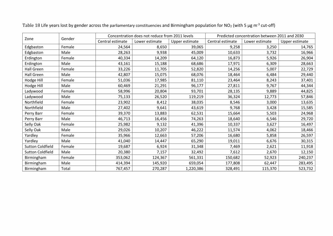
Table 18 Life years lost by gender across the parliamentary constituencies and Birmingham population for NO2 (with 5 μg m-3 cut-off)




Edgbaston Male 28,263 9,938 45,009 10,633 3,732 16,966


Erdington Male 43,161 15,188 68,686 17,971 6,309 28,663


Hall Green Male 42,807 15,075 68,076 18,464 6,484 29,440


Hodge Hill Male 60,469 21,291 96,177 27,811 9,767 44,344

Ladywood Female 58,996 20,804 93,701 28,135 9,889 44,825

Ladywood Male 75,133 26,520 119,219 36,324 12,773 57,846


Northfield Male 27,402 9,641 43,619 9,768 3,428 15,585


Perry Barr Male 46,713 16,456 74,263 18,640 6,546 29,720

Selly Oak Female 25,982 9,132 41,396 10,337 3,627 16,497

Selly Oak Male 29,026 10,207 46,222 11,574 4,062 18,466

Yardley Female 35,966 12,663 57,206 16,680 5,858 26,597

Yardley Male 41,040 14,447 65,290 19,011 6,676 30,315




Birmingham Male 414,394 145,920 659,054 177,808 62,447 283,495

Birmingham Total 767,457 270,287 1,220,386 328,491 115,370 523,732

Table 19 Annualised economic impact (in 2014 prices) across the parliamentary constituencies and Birmingham population for PM2.5 and NO2 (with 7

μg m-3 and 5 μg m-3 cut-off for PM2.5 and NO2, respectively)

Zone






Central estimate Central estimate Central estimate Central estimate

Edgbaston £23,069,783 £8,088,749 £30,264,686 £12,043,928

Erdington £33,592,790 £14,183,538 £47,182,867 £20,666,070

Hall Green £31,502,362 £11,432,109 £41,931,729 £18,766,104

Hodge Hill £43,272,635 £16,804,911 £59,741,837 £28,369,599

Ladywood £50,564,437 £22,806,055 £72,368,899 £35,697,933

Northfield £23,084,994 £7,432,709 £29,488,817 £11,206,998

Perry Barr £34,265,161 £15,084,249 £47,962,747 £19,984,928

Selly Oak £24,001,756 £7,853,300 £31,427,705 £13,147,583

Yardley £31,786,720 £11,689,665 £43,074,754 £20,755,045


Birmingham £313,958,210 £121,993,163 £427,680,084 £190,370,755

Table 20 Loss of life expectancy by gender across the parliamentary constituencies and Birmingham from birth in 2011 for anthropogenic PM2.5

(without cut-off) and NO2 (without cut-off)

Zone Gender Loss of life expectancy from birth compared with baseline mortality rates, 2011 birth cohort followed for 105 years (weeks)

Anthropogenic PM2.5 (without cut-off) NO2 (without cut-off)





Edgbaston Female 31.1 22.0 23.3 11.2

Edgbaston Male 36.7 25.8 27.5 13.2

Erdington Female 39.7 27.9 33.9 16.5

Erdington Male 44.5 31.3 38.0 18.5

Hall Green Female 31.0 21.8 24.0 12.6

Hall Green Male 38.3 26.9 29.7 15.5

Hodge Hill Female 37.5 26.0 31.3 16.8

Hodge Hill Male 44.8 31.1 37.4 20.0

Ladywood Female 40.7 28.9 36.3 19.7

Ladywood Male 48.1 34.2 43.0 23.4

Northfield Female 30.3 21.5 21.4 10.3

Northfield Male 35.9 25.5 25.3 12.1

Perry Barr Female 34.9 25.0 29.7 14.1

Perry Barr Male 42.1 30.1 35.8 17.0

Selly Oak Female 32.4 22.7 23.9 12.1

Selly Oak Male 37.0 26.0 27.3 13.8

Yardley Female 35.5 24.6 28.4 15.4

Yardley Male 39.8 27.6 31.9 17.3

Sutton Coldfield Female 28.4 20.0 20.8 9.9

Sutton Coldfield Male 31.8 22.4 23.4 11.1

Birmingham Female 34.9 24.6 28.4 14.5

Birmingham Male 40.9 28.8 33.2 17.0

Table 21 Loss of life expectancy by gender across the parliamentary constituencies and Birmingham from birth in 2011 for anthropogenic PM2.5 (with 7

μg m-3 cut-off) and NO2 (with 5 μg m-3 cut-off)

Zone Gender Loss of life expectancy from birth compared with baseline mortality rates, 2011 birth cohort followed for 105 years (weeks)

Anthropogenic PM2.5 (with 7 μg m-3 cut-off) NO2 (with 5 μg m-3 cut-off)





Edgbaston Female 14.0 4.4 18.3 6.1

Edgbaston Male 16.5 5.2 21.7 7.3

Erdington Female 20.1 7.9 28.2 10.8

Erdington Male 22.5 8.9 31.6 12.0

Hall Green Female 14.5 4.9 19.2 7.7

Hall Green Male 17.9 6.0 23.8 9.6

Hodge Hill Female 18.8 6.9 25.9 11.3

Hodge Hill Male 22.4 8.2 30.9 13.5

Ladywood Female 21.5 9.4 30.8 14.1

Ladywood Male 25.5 11.1 36.5 16.8

Northfield Female 12.8 3.6 16.3 5.1

Northfield Male 15.1 4.3 19.3 6.1

Perry Barr Female 17.7 7.4 24.8 9.1

Perry Barr Male 21.3 8.9 29.8 10.9

Selly Oak Female 14.3 4.2 18.7 6.8

Selly Oak Male 16.3 4.8 21.4 7.7

Yardley Female 17.0 5.8 23.1 10.0

Yardley Male 19.1 6.5 25.9 11.2

Sutton Coldfield Female 12.7 3.9 16.3 5.3

Sutton Coldfield Male 14.2 4.4 18.2 5.9

Birmingham Female 17.0 6.2 23.2 9.3

Birmingham Male 19.8 7.2 27.1 10.9

8.3 Additional tables – burden

Table 22 Estimated burden (from single-pollutant model summary estimate with wider estimates

of uncertainty) of effects on annual mortality in 2011 of 2011 levels of anthropogenic PM2.5 (with

and without cut-off)

Zone

Anthropogenic PM2.5 (without cut-off) Anthropogenic PM2.5 (with cut-off)


Lower estimate

Upper estimate

Central estimate

Lower estimate

Upper estimate

Edgbaston 48 8 90 22 4 41

Erdington 70 12 130 36 6 68

Hall Green 45 8 86 21 4 41

Hodge Hill 65 12 123 33 6 63

Ladywood 45 8 84 24 4 46

Northfield 51 9 97 22 4 42

Perry Barr 53 9 99 27 5 51

Selly Oak 57 10 108 26 4 49

Yardley 63 11 119 31 5 59


Birmingham 554 98 1,041 266 46 510 Using COMEAP’s recommended concentration-response coefficient of 1.06 per 10 μg m-3 of anthropogenic PM2.5 for the central estimate (lower estimate RR of 1.01 and upper estimate RR 1.12)

Table 23 Estimated burden (from the estimates derived by using information from multi-pollutant model results from 4 different cohort studies) of

effects on annual mortality in 2011 of 2011 levels of anthropogenic PM2.5 and NO2 (with cut-off), total population in each constituency in 2011,

mortality rate (total death age 30 plus divided by total population age 30 plus) in each constituency, ratio of the population age 65 and above over

the total population in each constituency and deprivation index Carstairs quintiles22

Zone


(without cut-off) Total population Mortality rate

(age group 30 plus) Ratio Population above 65 when

compared with total population

Carstairs quintile


derived from information in 4 studies below*)

Edgbaston 47 - 59 96,579 1.29% 14% 4.5

Erdington 75 - 91 97,791 1.62% 14% 5

Hall Green 46 - 57 115,921 1.07% 11% 4.5

Hodge Hill 69 - 85 121,700 1.49% 10% 5

Ladywood 50 - 60 126,713 1.03% 7% 5

Northfield 49 - 64 101,434 1.29% 15% 5

Perry Barr 56 - 69 107,105 1.20% 12% 4.75

Selly Oak 56 - 72 104,078 1.51% 14% 4.5

Yardley 65 - 81 95,115 1.45% 14% 5

Sutton Coldfield 56 - 72 106,753 1.31% 20% 2.25 *Using COMEAP’s recommended concentration-response coefficient of 1.029, 1.033, 1.053 and 1.019 per 10 μg m-3 of anthropogenic PM2.5 derived by applying to a single pollutant model summary estimate the % reduction in the coefficient on adjustment for nitrogen dioxide from the Jerrett et al (2013), Fischer et al (2015), Beelen et al (2014) and Crouse et al (2015) studies , respectively *Using COMEAP’s recommended concentration-response coefficient of 1.019, 1.016, 1.011 and 1.020 per 10 μg m-3 of NO2 derived by applying to a single pollutant model summary estimate the % reduction in the coefficient on adjustment for PM2.5 from the Jerrett et al (2013), Fischer et al (2015), Beelen et al (2014) and Crouse et al (2015) studies , respectively

22 Acknowledgement to Dr Daniela Fecht (Imperial College London) for formatting Carstair Quintiles data by Wards https://www.researchgate.net/publication/6817786_Measuring_deprivation_in_England_and_Wales_using_2001_Carstairs_scores

https://www.researchgate.net/publication/6817786_Measuring_deprivation_in_England_and_Wales_using_2001_Carstairs_scores

Table 24 Estimated burden (from multi pollutant study) of effects on annual mortality in 2011 of 2011 levels of anthropogenic PM2.5 and NO2

(without cut-off)

Zone

Anthropogenic PM2.5

(without cut-off) (not to be used separately)

NO2

(without cut-off) (not to be used separately)


(without cut-off) (combined estimate has less uncertainty)

Attributable deaths Attributable deaths Attributable deaths Jerrett Fischer Beelen Crouse Jerrett Fischer Beelen Crouse Jerrett Fischer Beelen Crouse

Edgbaston 24 27 42 16 30 25 17 31 54 52 59 47

Erdington 35 39 62 23 49 42 29 52 84 81 91 75

Hall Green 23 26 40 15 29 25 17 31 52 51 57 46

Hodge Hill 33 37 58 22 45 38 27 47 78 75 85 69

Ladywood 22 25 40 15 33 28 20 35 55 53 60 50

Northfield 26 29 46 17 31 26 18 32 57 55 64 49

Perry Barr 26 30 47 17 37 32 22 39 63 62 69 56

Selly Oak 29 32 51 19 35 30 21 37 64 62 72 56

Yardley 32 36 56 21 42 36 25 44 74 72 81 65

Sutton Coldfield 28 32 51 19 35 30 21 37 63 62 72 56

Birmingham 277 314 493 184 368 311 216 386 645 625 709 570 Using COMEAP’s recommended concentration-response coefficient of 1.029, 1.033, 1.053 and 1.019 per 10 μg m-3 of anthropogenic PM2.5 derived by applying to a single pollutant model summary estimate the % reduction in the coefficient on adjustment for nitrogen dioxide from the Jerrett et al (2013), Fischer et al (2015), Beelen et al (2014) and Crouse et al (2015) studies , respectively Using COMEAP’s recommended concentration-response coefficient of 1.019, 1.016, 1.011 and 1.020 per 10 μg m-3 of NO2 derived by applying to a single pollutant model summary estimate the % reduction in the coefficient on adjustment for PM2.5 from the Jerrett et al (2013), Fischer et al (2015), Beelen et al (2014) and Crouse et al (2015) studies , respectively

Table 25 Estimated burden (from multi pollutant study) of effects on annual mortality in 2011 of 2011 levels of anthropogenic PM2.5 and NO2 (with

cut-off)

Zone

Anthropogenic PM2.5

(with cut-off) (not to be used separately)

NO2

(with cut-off) (not to be used separately)


(with cut-off)

Attributable deaths Attributable deaths Attributable deaths Jerrett Fischer Beelen Crouse Jerrett Fischer Beelen Crouse Jerrett Fischer Beelen Crouse

Edgbaston 11 12 19 7 23 20 14 25 34 32 33 32

Erdington 18 20 32 12 41 35 24 43 59 55 56 55

Hall Green 11 12 19 7 24 20 14 25 35 32 33 32

Hodge Hill 16 18 29 11 37 32 22 39 53 50 51 50

Ladywood 12 14 21 8 28 24 17 30 40 38 38 38

Northfield 11 12 20 7 23 20 14 25 34 32 34 32

Perry Barr 13 15 24 9 31 26 18 33 44 41 42 42

Selly Oak 13 14 23 8 28 23 16 29 41 37 39 37

Yardley 15 17 27 10 34 29 20 36 49 46 47 46

Sutton Coldfield 13 14 23 8 28 23 16 29 41 37 39 37

Birmingham 132 150 237 87 298 252 175 313 430 402 412 400 Using COMEAP’s recommended concentration-response coefficient of 1.029, 1.033, 1.053 and 1.019 per 10 μg m-3 of anthropogenic PM2.5 derived by applying to a single pollutant model summary estimate the % reduction in the coefficient on adjustment for nitrogen dioxide from the Jerrett et al (2013), Fischer et al (2015), Beelen et al (2014) and Crouse et al (2015) studies , respectively Using COMEAP’s recommended concentration-response coefficient of 1.019, 1.016, 1.011 and 1.020 per 10 μg m-3 of NO2 derived by applying to a single pollutant model summary estimate the % reduction in the coefficient on adjustment for PM2.5 from the Jerrett et al (2013), Fischer et al (2015), Beelen et al (2014) and Crouse et al (2015) studies , respectively

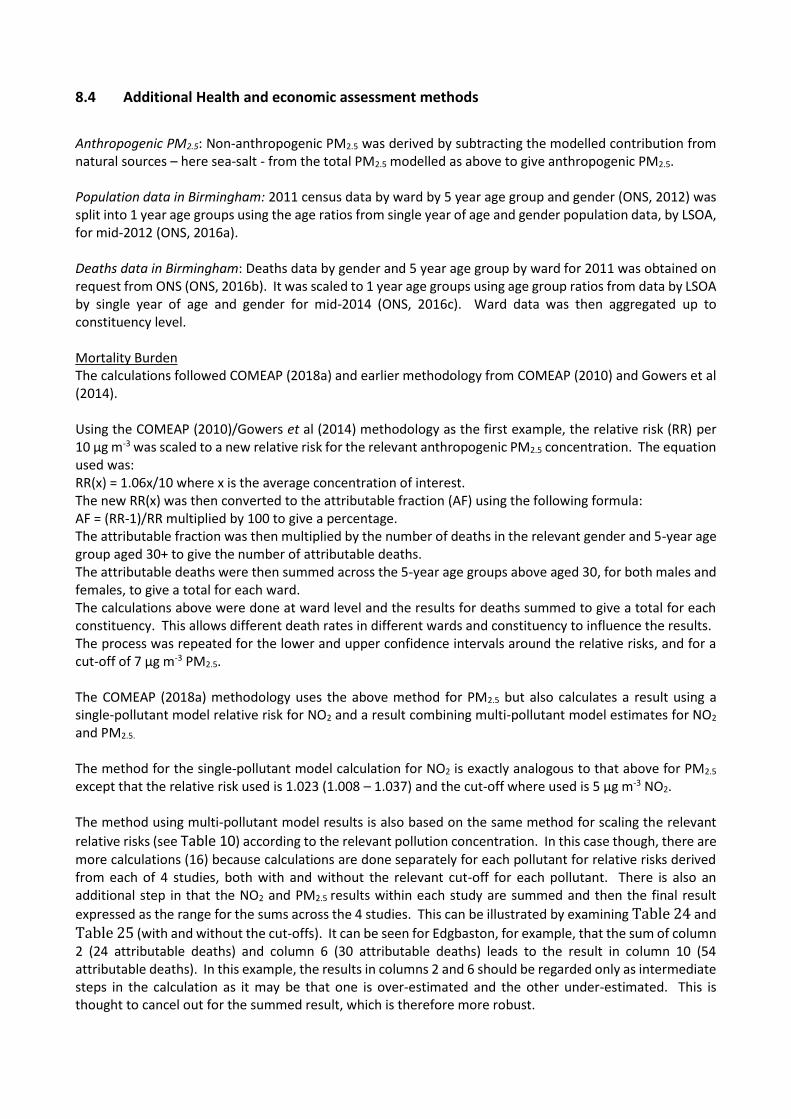
8.4 Additional Health and economic assessment methods

Anthropogenic PM2.5: Non-anthropogenic PM2.5 was derived by subtracting the modelled contribution from natural sources – here sea-salt - from the total PM2.5 modelled as above to give anthropogenic PM2.5. Population data in Birmingham: 2011 census data by ward by 5 year age group and gender (ONS, 2012) was split into 1 year age groups using the age ratios from single year of age and gender population data, by LSOA, for mid-2012 (ONS, 2016a). Deaths data in Birmingham: Deaths data by gender and 5 year age group by ward for 2011 was obtained on request from ONS (ONS, 2016b). It was scaled to 1 year age groups using age group ratios from data by LSOA by single year of age and gender for mid-2014 (ONS, 2016c). Ward data was then aggregated up to constituency level. Mortality Burden The calculations followed COMEAP (2018a) and earlier methodology from COMEAP (2010) and Gowers et al (2014). Using the COMEAP (2010)/Gowers et al (2014) methodology as the first example, the relative risk (RR) per 10 μg m-3 was scaled to a new relative risk for the relevant anthropogenic PM2.5 concentration. The equation used was: RR(x) = 1.06x/10 where x is the average concentration of interest. The new RR(x) was then converted to the attributable fraction (AF) using the following formula: AF = (RR-1)/RR multiplied by 100 to give a percentage. The attributable fraction was then multiplied by the number of deaths in the relevant gender and 5-year age group aged 30+ to give the number of attributable deaths. The attributable deaths were then summed across the 5-year age groups above aged 30, for both males and females, to give a total for each ward. The calculations above were done at ward level and the results for deaths summed to give a total for each constituency. This allows different death rates in different wards and constituency to influence the results. The process was repeated for the lower and upper confidence intervals around the relative risks, and for a cut-off of 7 μg m-3 PM2.5. The COMEAP (2018a) methodology uses the above method for PM2.5 but also calculates a result using a single-pollutant model relative risk for NO2 and a result combining multi-pollutant model estimates for NO2 and PM2.5.

The method for the single-pollutant model calculation for NO2 is exactly analogous to that above for PM2.5 except that the relative risk used is 1.023 (1.008 – 1.037) and the cut-off where used is 5 μg m-3 NO2. The method using multi-pollutant model results is also based on the same method for scaling the relevant

relative risks (see Table 10) according to the relevant pollution concentration. In this case though, there are more calculations (16) because calculations are done separately for each pollutant for relative risks derived from each of 4 studies, both with and without the relevant cut-off for each pollutant. There is also an additional step in that the NO2 and PM2.5 results within each study are summed and then the final result

expressed as the range for the sums across the 4 studies. This can be illustrated by examining Table 24 and

Table 25 (with and without the cut-offs). It can be seen for Edgbaston, for example, that the sum of column 2 (24 attributable deaths) and column 6 (30 attributable deaths) leads to the result in column 10 (54 attributable deaths). In this example, the results in columns 2 and 6 should be regarded only as intermediate steps in the calculation as it may be that one is over-estimated and the other under-estimated. This is thought to cancel out for the summed result, which is therefore more robust.

Mortality Impact Projections for the baseline life tables before applying concentration changes Natural change – current population size, age distributions and mortality rates will generate future changes in population and age structure in any case. We did not add this separately as it is already taken into account in our life table modelling. Changes in births over time – actual data on numbers of births in each local authority was used from 2011-2015 (ONS, 2016d), birth projections by local authority were used from 2016 to 2033 (ONS, 2016e) and the ratio of birth projections to 2039 births for England obtained from national populations projections (ONS, 2015a) was used to scale 2039 births in local authorities to local authority births for 2040 to 2114. No projections were available after 2114 so births were left constant for 2115 to 2134. Changes in births over time by constituency – births in each local authority as above was weighted by the 2011 birth data in each constituency aggregated from the population data in Birmingham by ward using 2011 census data (as above). Mortality rate improvements were applied to the 2011 all cause hazard rates according to the projected % improvements per year provided by ONS. Percentage improvements for different example ages are provided in Office for National Statistics (ONS, 2015b); we requested the full set of percentage improvements from ONS. Migration – predicting migration at the current time post the European referendum is particularly uncertain with both increases and decreases forecast. We did not therefore include this in our first analyses as presented in this report. Over the country as a whole this contribution to overall health impacts is likely to be small. This can be explored further in future work. Lags: The approach allowed for a delay between exposure and effect using the recommended distribution of lags from COMEAP (COMEAP, 2010) i.e. 30% of the effect in the first year, 12.5% in each of years 2-5 and 20% spread over years 5-20. An analogous approach was used for the effects of long-term exposure to NO2. HRAPIE (WHO, 2013) recommended that, in the absence of information on likely lags between long-term exposure to NO2 and mortality, calculations should follow whatever lags are chosen for PM2.5. Calculations

The relative risk (RR) per 10 μg m-3 was scaled to a new relative risk for the appropriate population-weighted

mean for each gender in each parliamentary constituency for each scenario and year. The equation used (for the example coefficient of 1.06) was: RR(x) = 1.06x/10 where x is the concentration of interest (with a negative sign for a reduction). Concentrations were assumed to reduce linearly between the years in which modelled concentrations were available (2011, 2015, 2020, 2025, 2030). The scaled RR was then used to adjust the all cause hazard rates in the life table calculations. For the 5 μg m-3 cut-off for NO2, ward concentrations were interpolated between 2011, 2015, 2020, 2025 and 2030 and 5 μg m-3 was then subtracted from the ward concentrations in each year. Any resulting negative concentrations were then set to zero before all the ward concentrations were population-weighted to local authority level as normal. Life table calculations were programmed in SQL based on the methods used in the standard IOMLIFET spreadsheets 132 with the following amendments:

- Extension to 2134 (105 years after 2030) - Adjustment of the baseline hazard rates over time according to projected mortality rate

improvements - Inclusion of changes in numbers of births over time - IOMLIFET excludes neonatal deaths. We included neonatal deaths and followed the South East Public

Health Observatory life-expectancy calculator23 and Gowers et al. (2014) in taking into account the uneven distribution of deaths over the course of the first year when calculating the survival probability. (The survival probability (the ratio of the number alive at the end of the year to the number alive at the beginning) is derived by the equivalent of adding half the deaths back onto the mid-year population to give the starting population and subtracting half the deaths from the mid-

23 https://webarchive.nationalarchives.gov.uk/20130329125326/http://www.lho.org.uk/viewResource.aspx?id=8943&sUri=http%3a%2f%2fwww.sepho.org.uk%2f

https://webarchive.nationalarchives.gov.uk/20130329125326/http:/www.lho.org.uk/viewResource.aspx?id=8943&sUri=http%3a%2f%2fwww.sepho.org.uk%2f

https://webarchive.nationalarchives.gov.uk/20130329125326/http:/www.lho.org.uk/viewResource.aspx?id=8943&sUri=http%3a%2f%2fwww.sepho.org.uk%2f

year population to give the end population, assuming deaths are distributed evenly across the year. This is not the case in the first year where a weighting factor based on 90% of the deaths occurring in the first half of the year and 10% in the second half is used instead. After rearrangement the actual formula is (1- 0.1 x hazard rate)/(1+ 0.9 x hazard rate) rather than the (1- 0.5 x hazard rate)/(1+ 0.5 x hazard rate) used in other years.)

Results for total and annual life years lost by parliamentary constituency were then summed to

Birmingham level. We also used the life tables to calculate changes in life expectancy. Economic valuation24 The approach taken here is based on the discipline of environmental economics (ExternE, 2005). Environmental economics was developed partly in response to recognition of the externalities, or external costs, posed by various human activities. ‘Externalities’ are unforeseen effects that arise from action that benefits one party generally to the detriment of others, when those effects are external, or not considered, in the decision-making process. Notable examples include the loss of utility from effects of air pollution arising from power generation or transport. The question faced by the economist in this situation is not how to allocate a defined amount of resource (the health service budget), but how much should be spent to mitigate externalities. This requires that health impacts are monetised in order that the benefits of action can be compared directly with the costs in a benefit-cost analysis. Several approaches have been taken to value mortality impacts (the impacts that dominate the assessment made in this report), though all seek to quantify public preference, demonstrating consistency in objective with the health economics work in deriving QALYs for various conditions. The methods used for valuing a death fall into three categories: Wage-risk studies, which consider the additional wage demanded of people working in risky occupations, providing an estimate of willingness to accept (WTA) risk. Consumer market studies, that consider the willingness of individuals to pay (WTP) for equipment that will reduce their risk of death. Several studies were carried out on car safety equipment (air bags, etc.) before they were made mandatory. Contingent valuation (CV) surveys, where individuals are asked for their WTP for treatments that will reduce the risk of a health impact of some kind, or of dying within X years. Early work in this field was affected by various biases. Considerable effort has been taken over the last three decades to identify these biases and refine CV approaches to reduce them, with some success. In the context of health valuation, the underlying calculations are similar whichever of the three methods just mentioned is used. In the case of the wage risk studies, for example, it may be observed that construction workers operating at height will accept an additional risk of death annually of 1 in 1,000 (0.001), for an additional wage of £1000. The value of statistical life (VSL) calculated from these figures would be £1000/0.001 - £1,000,000. A review by OECD gives an averaged VSL for EU Member States of €3million. UK Government, via the Department for Transport, adopts a value that is lower by about 40% of £1.56 million (DfT, 2017). Opinion is divided as to whether valuation of mortality should concern ‘deaths’ or ‘life years lost’. The OECD is firmly committed to use of the VSL (OECD, 2012). UK government, through the Interdepartmental Group on Costs and Benefits, however, values mortality in terms of the loss of life expectancy expressed as the ‘Value of a Life Year’ (VOLY), taking a value of £36,379 in 2014 prices. The basic approach to quantification, however, is the same, with values elicited against a change in the risk of a health outcome, in this case, the loss of a life year. The large difference between the unit values for VSL and VOLY is partly mitigated in subsequent analysis by the number of life years lost being about 10 times higher than the number of deaths. However, the UK government position generates estimates of air pollution damage that are significantly lower than estimates made using the OECD position. Given that the UK government position is followed here, results should be considered to be at the conservative end of plausible ranges. Similar calculations can be made to assess the WTP to avoid ill health more generally, such as development of respiratory or cardiovascular disease. The total impact for morbidity has a number of elements:

24 Much of this section is sourced from text written by Mike Holland in Williams et al (2018b).

WTP to avoid lost utility (being well, and enjoying the opportunities that good health offers) The costs of health care Costs to the marketed economy through lost productivity Costs have been defined for a variety of endpoints of relevance to air pollution in analysis for UK government and also for other bodies, such as the European Commission (Holland, 2014a and 2014b). Adopted values, discounting and uplift The values of most relevance concern acute and chronic mortality, as these have been shown by numerous studies to dominate the CBA. The value of a lost year of life to chronic exposure as applied in the current analysis is £36,379, assuming that it reflects the loss of a year of life in ‘normal health’ taken from the guidance issued by Defra (2019). It is important to factor the time at which impacts occur into the analysis for two reasons. The first is that values should be uplifted for future years to capture the likely effect of (anticipated) growth in incomes on WTP for health protection. The second, opposing effect, concerns the need to discount future values on the basis that money or goods are more valuable now than at some point in the future. There are several reasons for this. One is that resource available now can be used to increase the availability of resource in the future. An obvious example concerns investment in infrastructure projects that facilitate economic development. Along similar lines, investment in health research may lead to the development of cures or treatments for illnesses in the future. Further information can be found in Guidance from Her Majesty’s Treasury in the ‘Green Book’ (HMT, 2018). The Green Book recommends the use of declining discount rates for effects quantified over prolonged periods. However, the impact of using declining discount rates in line with the HMT recommendation, rather than constant discount rates, will be minimal as they apply only after 30 years have passed, by which time values are reduced by two thirds. The impact of the declining rates will clearly increase over time, though

the rate of decline (see Table 26) is so slight this will still make little difference.

Table 26 Schedule of declining long-term discount rates from HMT, 2018

Period of years Discount rate

0 – 30 3.5%

31 – 75 3.0%

76 – 125 2.5%

126 – 200 2.0%

201 – 300 1.5%

301+ 1.0%

The government guidance (HMT, 2019) recommends that future values should be uplifted at 2% per annum given that “It is expected that as people’s incomes rise, so too does their willingness to pay to reduce health risks such as those associated with air pollution.” However, it is unclear whether the uplift of 2% is still appropriate. It is notable that it was first developed before the economic crash of 2008, and so does not account for any change in growth since that time. However, the present analysis is based on a long time-frame, so short-term perturbations to growth seem likely to be factored out in the longer term. Inequality is not factored explicitly into the economic analysis, beyond the acceptance of a national average estimate for mortality valuation (in other words, the values of disadvantaged groups are not down rated to reflect a likely lower WTP linked to reduced ability to pay).

9.0 References

Beelen, R., Raaschou-Nielsen, O., Stafoggia, M., Andersen, Z. J., Weinmayr, G., Hoffmann, B., Wolf, K., Samoli, E., Fischer, P., Nieuwenhuijsen, M., Vineis, P., Xun, W. W., Katsouyanni, K., Dimakopoulou, K., Oudin, A., Forsberg, B., Modig, L., Havulinna, A. S., Lanki, T., Turunen, A., Oftedal, B., Nystad, W., Nafstad, P., De Faire, U., Pedersen, N. L., Ostenson, C. G., Fratiglioni, L., Penell, J., Korek, M., Pershagen, G., Eriksen, K. T., Overvad, K., Ellermann, T., Eeftens, M., Peeters, P. H., Meliefste, K., Wang, M., Bueno-De-Mesquita, B., Sugiri, D., Kramer, U., Heinrich, J., De Hoogh, K., Key, T., Peters, A., Hampel, R., Concin, H., Nagel, G., Ineichen, A., Schaffner, E., ProbstHensch, N., Kunzli, N., Schindler, C., Schikowski, T., Adam, M., Phuleria, H., Vilier, A., Clavel-Chapelon, F., Declercq, C., Grioni, S., Krogh, V., Tsai, M. Y., Ricceri, F., Sacerdote, C., Galassi, C., Migliore, E., Ranzi, A., Cesaroni, G., Badaloni, C., Forastiere, F., Tamayo, I., Amiano, P., Dorronsoro, M., Katsoulis, M., Trichopoulou, A., Brunekreef, B. & Hoek, G. 2014. Effects of long-term exposure to air pollution on natural-cause mortality: an analysis of 22 European cohorts within the multicentre ESCAPE project. The Lancet, 383, 785-95.

Chilton S, Covey J, Jones-Lee M, Loomes G and Metcalf H (2004) Valuation of health benefits associated with reductions in air pollution. Department for Environment, Food and Rural Affairs, London. Available at:

randd.defra.gov.uk/Document.aspx?Document=EP01006_4723_FRP.pdf

COMEAP (Committee on the Medical Effects of Air Pollutants), 2010, The mortality effects of long-term exposure to particulate matter air pollution in the UK, London, UK. Available at http://comeap.org.uk/documents/reports/128-the-mortality-effects-of-long-term-exposure-to-particulate-air-pollution-in-the-uk.html. (Accessed 7 June 2019).

COMEAP (2015) Interim Statement on Quantifying the Association of Long-Term Average Concentrations of Nitrogen Dioxide and Mortality. https://www.gov.uk/government/publications/nitrogen-dioxide-interim-view-on-long-term-average-concentrations-and-mortality. (Accessed 7 June 2019).

COMEAP (2016) Minutes of the meeting held on Wednesday 24th February 2016 COMEAP/2016/MIN/1 ‘Choice of cut-off’ under Item 5. Available from https://www.gov.uk/government/groups/committee-on-the-medical-effects-of-air-pollutants-comeap#minutes. (Accessed 7 June 2019).

COMEAP (2017) Annex A in Technical Report to Department for Environment Food & Rural Affairs (DEFRA). Air quality plan for nitrogen dioxide (NO2) in the UK, 2017, ‘UK Plan for tackling roadside nitrogen dioxide concentrations – technical report’. https://assets.publishing.service.gov.uk/government/uploads/system/uploads/attachment_data/file/632916/air-quality-plan-technical-report.pdf. (Accessed 7 June 2019).

COMEAP (2018a). Associations of long-term average concentrations of nitrogen dioxide with mortality. A report by the Committee on the Medical Effects of Air Pollutants. https://assets.publishing.service.gov.uk/government/uploads/system/uploads/attachment_data/file/734799/COMEAP_NO2_Report.pdf. (Accessed 7 June 2019).

COMEAP (2018b) Statement on quantifying mortality associated with long-term average concentrations of fine particulate matter (PM2.5) Available at: https://www.gov.uk/government/publications/particulate-air-pollution-effects-on-mortality. (Accessed 11 June 2019)

Crouse, D. L., Peters, P. A., Hystad, P., Brook, J. R., Van Donkelaar, A., Martin, R. V., Villeneuve, P. J., Jerrett, M., Goldberg, M. S. & Pope Iii, C. A. 2015a. Ambient PM2. 5, O3, and NO2 exposures and associations with mortality over 16 years of follow-up in the Canadian Census Health and Environment Cohort (CanCHEC). Environmental Health Perspectives, 123, 1180.

Dajnak D, Walton H, Smith J D and Beevers S (June 2018). Greater Manchester Health and Economic Impact Assessment study. This report was produced by King’s College London for IPPR North. ATMOSPHERE TOWARDS A PROPER STRATEGY FOR TACKLING GREATER MANCHESTER’S AIR POLLUTION CRISIS (June 2018). IPPR North; Ed Cox and Dom Goggins. https://www.ippr.org/publications/atmosphere. (Accessed 7 June 2019).

Defra (2019) Impact Pathways Approach Guidance for Air Quality Appraisal. https://assets.publishing.service.gov.uk/government/uploads/system/uploads/attachment_data/file/770649/impact-pathway-approach-guidance.pdf. (Accessed 7 June 2019).

https://eur03.safelinks.protection.outlook.com/?url=http%3A%2F%2Frandd.defra.gov.uk%2FDocument.aspx%3FDocument%3DEP01006_4723_FRP.pdf&data=01%7C01%7Cheather.walton%40kcl.ac.uk%7C64733ee0fe7344ca4ac108d6f621fbca%7C8370cf1416f34c16b83c724071654356%7C0&sdata=cWJ8346F%2Fu%2FTJ2S0E%2F%2F44B3lk0E0vi4aSA592MMu6EM%3D&reserved=0

http://comeap.org.uk/documents/reports/128-the-mortality-effects-of-long-term-exposure-to-particulate-air-pollution-in-the-uk.html

http://comeap.org.uk/documents/reports/128-the-mortality-effects-of-long-term-exposure-to-particulate-air-pollution-in-the-uk.html

https://www.gov.uk/government/publications/nitrogen-dioxide-interim-view-on-long-term-average-concentrations-and-mortality

https://www.gov.uk/government/publications/nitrogen-dioxide-interim-view-on-long-term-average-concentrations-and-mortality

https://www.gov.uk/government/groups/committee-on-the-medical-effects-of-air-pollutants-comeap#minutes

https://www.gov.uk/government/groups/committee-on-the-medical-effects-of-air-pollutants-comeap#minutes

https://assets.publishing.service.gov.uk/government/uploads/system/uploads/attachment_data/file/632916/air-quality-plan-technical-report.pdf

https://assets.publishing.service.gov.uk/government/uploads/system/uploads/attachment_data/file/632916/air-quality-plan-technical-report.pdf

https://assets.publishing.service.gov.uk/government/uploads/system/uploads/attachment_data/file/734799/COMEAP_NO2_Report.pdf

https://assets.publishing.service.gov.uk/government/uploads/system/uploads/attachment_data/file/734799/COMEAP_NO2_Report.pdf

https://www.gov.uk/government/publications/particulate-air-pollution-effects-on-mortality

https://www.gov.uk/government/publications/particulate-air-pollution-effects-on-mortality

https://www.ippr.org/publications/atmosphere

https://assets.publishing.service.gov.uk/government/uploads/system/uploads/attachment_data/file/770649/impact-pathway-approach-guidance.pdf

https://assets.publishing.service.gov.uk/government/uploads/system/uploads/attachment_data/file/770649/impact-pathway-approach-guidance.pdf

DfT (Department for Transport) (2017) Transport Analysis Guidance (TAG), March 2017. https://www.gov.uk/government/uploads/system/uploads/attachment_data/file/603277/webtag-databook-march-2017-release-v1-7.xls. (Accessed 7 June 2019).

ExternE (2005) ExternE – Externalities of Energy, Methodology 2005 update. http://www.externe.info/externe_d7/sites/default/files/methup05a.pdf. (Accessed 7 June 2019).

Fischer, P. H., Marra, M., Ameling, C. B., Hoek, G., Beelen, R., De Hoogh, K., Breugelmans, O., Kruize, H., Janssen, N. A. & Houthuijs, D. 2015. Air Pollution and Mortality in Seven Million Adults: The Dutch Environmental Longitudinal Study (DUELS). Environmental Health Perspectives, 123, 697-704.Fung K and Krewski D 1999. On Associations of long-term average concentrations of nitrogen dioxide with mortality 112 measurement error adjustment methods in poisson regression. Environmetrics 10, 213- 224.

Gowers A, Miller BG, Stedman JR, Estimating the mortality burdens associated with particulate air pollution, Public Health England, Report number PHE-CRCE-010, 2014. https://www.gov.uk/government/uploads/system/uploads/attachment_data/file/332854/PHE_CRCE_010.pdf http://www.hpa.org.uk/Publications/Environment/PHECRCEReportSeries/PHECRCE010/. (Accessed 7 June 2019).

HMT (2019) Valuing impacts on air quality: May 2013 Supplementary Green Book guidance. HM Treasury. https://www.gov.uk/government/publications/the-green-book-appraisal-and-evaluation-in-central-governent. (Accessed 7 June 2019).

HMT (2018). The Green Book: appraisal and evaluation in central government. Published by HMT. https://assets.publishing.service.gov.uk/government/uploads/system/uploads/attachment_data/file/685903/The_Green_Book.pdf. (Accessed 7 June 2019).

Hoek, G., Krishnan, R. M., Beelen, R., Peters, A., Ostro, B., Brunekreef, B. & Kaufman, J. D. 2013. Long-term air pollution exposure and cardio- respiratory mortality: a review. Environ Health, 12, 43.

Holland, M. (2014a) Implementation of the HRAPIE Recommendations for European Air Pollution CBA work. Report to European Commission DG Environment. January 2014.

Holland, M. (2014b) Cost-benefit analysis of final policy scenarios for the EU Clean Air Package. Corresponding to IIASA TSAP report no.11. Report to European Commission DG Environment. March 2014. http://ec.europa.eu/environment/air/pdf/TSAP%20CBA.pdf. (Accessed 7 June 2019).

IOM (2013) IOMLIFET: A Spreadsheet System For Life table Calculations For Health Impact Assessment Available at:

https://www.iom-world.org/research/our-expertise/iomlifet/. (Accessed 7 June 2019). (Accessed 7 June 2019).

Jerrett, M., Burnett, R. T., Beckerman, B. S., Turner, M. C., Krewski, D., Thurston, G., Martin, R. V., Van Donkelaar, A., Hughes, E., Shi, Y., Gapstur, S. M., Thun, M. J. & Pope, C. A., 3rd 2013. Spatial analysis of air pollution and mortality in California. Am J Respir Crit Care Med, 188, 593-9.Kim, J.Y., et al., 2007. Panel discussion review: session two-- interpretation of observed associations between multiple ambient air pollutants and health effects in epidemiologic analyses. J Expo Sci Environ Epidemiol 17 Suppl 2, S83-9. doi: 10.1038/sj.jes.750062

Morgan, O. and A. Baker (2006). "Measuring deprivation in England and Wales using 2001 Carstairs scores." Health Statistics Quarterly 31: 28-33.

OECD (2012) Mortality Risk Valuation in Environment, Health and Transport Policies. OECD, Paris.

ONS (Office for National Statistics) (2012) Dataset(s):2011 Census: Population and Household Estimates for Wards and Output Areas in England and Wales https://www.ons.gov.uk/peoplepopulationandcommunity/populationandmigration/populationestimates/datasets/2011censuspopulationandhouseholdestimatesforwardsandoutputareasinenglandandwales. (Accessed 7 June 2019).

ONS - Office for National Statistics (2015a) All data related to national population projections 2014-based statistical bulletin https://www.ons.gov.uk/peoplepopulationandcommunity/populationandmigration/populationprojections/bulletins/nationalpopulationprojections/2015-10-29/relateddata. (Accessed 7 June 2019).

https://www.gov.uk/government/uploads/system/uploads/attachment_data/file/603277/webtag-databook-march-2017-release-v1-7.xls

https://www.gov.uk/government/uploads/system/uploads/attachment_data/file/603277/webtag-databook-march-2017-release-v1-7.xls

http://www.externe.info/externe_d7/sites/default/files/methup05a.pdf

https://www.gov.uk/government/uploads/system/uploads/attachment_data/file/332854/PHE_CRCE_010.pdf

http://www.hpa.org.uk/Publications/Environment/PHECRCEReportSeries/PHECRCE010/

https://www.gov.uk/government/publications/the-green-book-appraisal-and-evaluation-in-central-governent

https://assets.publishing.service.gov.uk/government/uploads/system/uploads/attachment_data/file/685903/The_Green_Book.pdf

https://assets.publishing.service.gov.uk/government/uploads/system/uploads/attachment_data/file/685903/The_Green_Book.pdf

http://ec.europa.eu/environment/air/pdf/TSAP%20CBA.pdf

https://www.iom-world.org/research/our-expertise/iomlifet/

https://www.ons.gov.uk/peoplepopulationandcommunity/populationandmigration/populationestimates/datasets/2011censuspopulationandhouseholdestimatesforwardsandoutputareasinenglandandwales

https://www.ons.gov.uk/peoplepopulationandcommunity/populationandmigration/populationestimates/datasets/2011censuspopulationandhouseholdestimatesforwardsandoutputareasinenglandandwales

https://www.ons.gov.uk/peoplepopulationandcommunity/populationandmigration/populationprojections/bulletins/nationalpopulationprojections/2015-10-29/relateddata

https://www.ons.gov.uk/peoplepopulationandcommunity/populationandmigration/populationprojections/bulletins/nationalpopulationprojections/2015-10-29/relateddata

ONS - Office for National Statistics (2015b) Compendium: Mortality assumptions (2014-based national population projections) http://www.ons.gov.uk/peoplepopulationandcommunity/populationandmigration/populationprojections/compendium/nationalpopulationprojections/2015-10-29/mortalityassumptions. (Accessed 7 June 2019).

ONS - Office for National Statistics (2016a) Dataset: Lower Super Output Area Mid-Year Population Estimates (supporting information) https://www.ons.gov.uk/peoplepopulationandcommunity/populationandmigration/populationestimates/datasets/lowersuperoutputareamidyearpopulationestimates. (Accessed 7 June 2019). 110 Office for National Statistics (2016b) VS4: Births and Mortality data by ward; 2011 Email to H Walton 5/8/2016.

ONS - Office for National Statistics (2016c) User requested data: Deaths by LSOA, single year of age and sex, England and Wales, 2014 registrations https://www.ons.gov.uk/peoplepopulationandcommunity/birthsdeathsandmarriages/deaths/adhocs/005453deathsbylsoasingleyearofageandsexenglandandwales2014registrations. (Accessed 7 June 2019).

ONS - Office for National Statistics (2016d) Dataset: Births by mothers’ usual area of residence in the UK. https://www.ons.gov.uk/peoplepopulationandcommunity/birthsdeathsandmarriages/livebirths/datasets/birthsbyareaofusualresidenceofmotheruk. (Accessed 7 June 2019).

ONS - Office for National Statistics (2016e) Sub-national population projections, local authorities in England SNPP Z1 – 2014 based https://www.ons.gov.uk/peoplepopulationandcommunity/populationandmigration/populationprojections/datasets/localauthoritiesinenglandz1. (Accessed 7 June 2019).

Walton H, Dajnak D, Beevers SD, Williams ML, Watkiss P, Hunt A, Understanding the Health Impacts of Air Pollution in London, King’s College London 2015 available at: https://www.london.gov.uk/sites/default/files/hiainlondon_kingsreport_14072015_final.pdf. (Accessed 7 June 2019).

Williams ML, Lott MC, Kitwiroon N, Dajnak D, Walton H, Holland M, Pye S, Fecht D, Toledano MB, Beevers SD (2018a) The Lancet Countdown on health benefits from the UK Climate Change Act: a modelling study for Great Britain. Lancet Planetary Health 2 (5): e202-e213

Williams ML, Lott MC, Kitwiroon N, Dajnak D, Walton H, Holland M, Pye S, Fecht D, Toledano MB, Beevers SD (2018b) Public health air pollution impacts of different pathways to meet the UK Climate Change Act commitment to 80% reduction on CO2 and other greenhouse gas emissions by 2050. Full report in press, summary at https://www.journalslibrary.nihr.ac.uk/programmes/phr/11300513/#/. (Accessed 7 June 2019).

World Health Organisation (2013), Health risks of air pollution in Europe-HRAPIE project, WHO Regional office for Europe,. Available at:http://www.euro.who.int/en/health-topics/environment-and-health/air-quality/publications/2013/health-risks-of-air-pollution-in-europe-hrapie-project.-recommendations-for-concentrationresponse-functions-for-costbenefit-analysis-of-particulate-matter,-ozone-and-nitrogen-dioxide. (Accessed 7 June 2019).

https://emea01.safelinks.protection.outlook.com/?url=http%3A%2F%2Fwww.ons.gov.uk%2Fpeoplepopulationandcommunity%2Fpopulationandmigration%2Fpopulationprojections%2Fcompendium%2Fnationalpopulationprojections%2F2015-10-29%2Fmortalityassumptions&data=01%7C01%7Cheather.walton%40kcl.ac.uk%7C82bb8170be61441d74d308d41907170e%7C8370cf1416f34c16b83c724071654356%7C0&sdata=lkpL41nFBUBQqNQu5MK6yPNbdfyXNsJt7BDf1gNS5Xc%3D&reserved=0

https://emea01.safelinks.protection.outlook.com/?url=http%3A%2F%2Fwww.ons.gov.uk%2Fpeoplepopulationandcommunity%2Fpopulationandmigration%2Fpopulationprojections%2Fcompendium%2Fnationalpopulationprojections%2F2015-10-29%2Fmortalityassumptions&data=01%7C01%7Cheather.walton%40kcl.ac.uk%7C82bb8170be61441d74d308d41907170e%7C8370cf1416f34c16b83c724071654356%7C0&sdata=lkpL41nFBUBQqNQu5MK6yPNbdfyXNsJt7BDf1gNS5Xc%3D&reserved=0

https://www.ons.gov.uk/peoplepopulationandcommunity/populationandmigration/populationestimates/datasets/lowersuperoutputareamidyearpopulationestimates

https://www.ons.gov.uk/peoplepopulationandcommunity/populationandmigration/populationestimates/datasets/lowersuperoutputareamidyearpopulationestimates

https://www.ons.gov.uk/peoplepopulationandcommunity/birthsdeathsandmarriages/deaths/adhocs/005453deathsbylsoasingleyearofageandsexenglandandwales2014registrations

https://www.ons.gov.uk/peoplepopulationandcommunity/birthsdeathsandmarriages/deaths/adhocs/005453deathsbylsoasingleyearofageandsexenglandandwales2014registrations

https://www.ons.gov.uk/peoplepopulationandcommunity/birthsdeathsandmarriages/livebirths/datasets/birthsbyareaofusualresidenceofmotheruk

https://www.ons.gov.uk/peoplepopulationandcommunity/birthsdeathsandmarriages/livebirths/datasets/birthsbyareaofusualresidenceofmotheruk

https://www.ons.gov.uk/peoplepopulationandcommunity/populationandmigration/populationprojections/datasets/localauthoritiesinenglandz1

https://www.ons.gov.uk/peoplepopulationandcommunity/populationandmigration/populationprojections/datasets/localauthoritiesinenglandz1

https://www.london.gov.uk/sites/default/files/hiainlondon_kingsreport_14072015_final.pdf

https://kclpure.kcl.ac.uk/portal/martin.williams.html

https://kclpure.kcl.ac.uk/portal/heather.walton.html

https://kclpure.kcl.ac.uk/portal/sean.beevers.html

https://kclpure.kcl.ac.uk/portal/en/journals/lancet-planetary-health(772f4513-b09e-4e4d-8cfe-2bee577cb195).html

https://kclpure.kcl.ac.uk/portal/en/journals/lancet-planetary-health(772f4513-b09e-4e4d-8cfe-2bee577cb195).html

https://kclpure.kcl.ac.uk/portal/martin.williams.html

https://kclpure.kcl.ac.uk/portal/heather.walton.html

https://kclpure.kcl.ac.uk/portal/sean.beevers.html

https://www.journalslibrary.nihr.ac.uk/programmes/phr/11300513/#/

http://www.euro.who.int/en/health-topics/environment-and-health/air-quality/publications/2013/health-risks-of-air-pollution-in-europe-hrapie-project.-recommendations-for-concentrationresponse-functions-for-costbenefit-analysis-of-particulate-matter,-ozone-and-nitrogen-dioxide



birmingham city health and economic impact assessment … executive summary and key results uk100...

Documents