bionet tutorial - bioconductor · october 30, 2018 abstract the rst part of this tutorial exempli...

BioNet Tutorial

Daniela Beisser and Marcus Dittrich

May 2, 2019

Abstract

The first part of this tutorial exemplifies how an integrated networkanalysis can be conducted using the BioNet package. Here we will inte-grate gene expression data from different lymphoma subtypes and clinicalsurvival data with a comprehensive protein-protein interaction (PPI) net-work based on HPRD. This is shown first in a quick start and later in amore detailed analysis. The second part will focus on the integration ofgene expression data from Affymetrix single-channel microarrays with thehuman PPI network.

1 Quick Start

The quick start section gives a short overview of the essential BioNet methodsand their application. A detailed analysis of the same data set of diffuse largeB-cell lymphomas is presented in section 3 .The major aim of the presented integrated network analysis is to identify mod-ules, which are differentially expressed between two different lymphoma sub-types (ABC and GCB) and simultaneously are risk associated (measured by thesurvival analysis).First of all, we load the BioNet package and the required data sets, containing ahuman protein-protein interaction network and p-values derived from differentialexpression and survival analysis.

> library(BioNet)

> library(DLBCL)

> data(dataLym)

> data(interactome)

Then we need to aggregate these two p-values into one p-value.

> pvals <- cbind(t = dataLym$t.pval, s = dataLym$s.pval)

> rownames(pvals) <- dataLym$label

> pval <- aggrPvals(pvals, order = 2, plot = FALSE)

Next a subnetwork of the complete network is derived, containing all the pro-teins which are represented by probesets on the microarray. And self-loops areremoved.

> subnet <- subNetwork(dataLym$label, interactome)

> subnet <- rmSelfLoops(subnet)

> subnet

1

A graphNEL graph with undirected edges

Number of Nodes = 2559

Number of Edges = 7788

To score each node of the network we fit a Beta-uniform mixture model (BUM)[10] to the p-value distribution and subsequently use the parameters of the modelfor the scoring function [5]. A false-discovery rate (FDR) of 0.001 is chosen.

> fb <- fitBumModel(pval, plot = FALSE)

> scores <- scoreNodes(subnet, fb, fdr = 0.001)

Here we use a fast heuristic approach to calculate an approximation to theoptimal scoring subnetwork. An optimal solution can be calculated using theheinz algorithm [5] requiring a commercial CPLEX license, see section 3.4 and6 for installation.

> module <- runFastHeinz(subnet, scores)

> logFC <- dataLym$diff

> names(logFC) <- dataLym$label

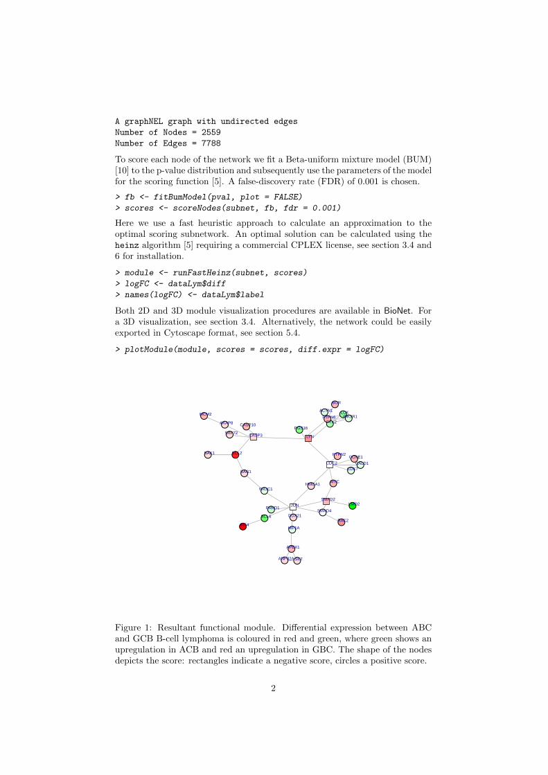
Both 2D and 3D module visualization procedures are available in BioNet. Fora 3D visualization, see section 3.4. Alternatively, the network could be easilyexported in Cytoscape format, see section 5.4.

> plotModule(module, scores = scores, diff.expr = logFC)

●

●

● ●

●

●

●

●

●

●

●

●

●

●

●

●●

●

●

●

●

●

●●

●

●

●

●

●

●●

●

ACTN1

APEX1

BAK1 BCL2

BAG1

BCL6

BCR

CALD1

CASP3

CASP10

CCNE1

CDC2CDK7

NR3C1

HIF1A

HMGA1

JUN

LCK

LMO2

LYN

SMAD2

SMAD4

MCM2

IRF4

MYC

PIK3R1

PRKD1

PTK2PTPN6

RAC2

SET

PTPN2

RGS16

ANP32A

AKAP8

SRP72

DDX21

Figure 1: Resultant functional module. Differential expression between ABCand GCB B-cell lymphoma is coloured in red and green, where green shows anupregulation in ACB and red an upregulation in GBC. The shape of the nodesdepicts the score: rectangles indicate a negative score, circles a positive score.

2

2 Heuristics to Calculate High-scoring Subnet-works

To calculate high-scoring subnetworks without an available CPLEX license aheuristics is included in the BioNet package. The following depicts a shortoutline of the algorithm:

1. In the first step all positive connected nodes are aggregated into meta-nodes.

2. By defining an edge score based on the node’s scores that are on theendpoints of an edge, the node scores are transfered to the edges.

3. On these edge scores a minimum spanning tree (MST) is calculated.

4. All paths between positive meta-nodes are calculated based on the MSTto obtain the negative nodes between the positives.

5. Upon these negative nodes again a MST is calculated from which thepath with the highest score, regarding node scores of negative nodes andthe positive meta-nodes they connect, gives the resulting approximatedmodule.

To validate the performance of the heuristic we simulate artificial signal mod-ules. For this we use the induced subnetwork of the HPRD-network comprisingthe genes present on the hgu133a Affymetrix chip. Within this network weset artificial signal modules of biological relevant sizes of 30 and 150 nodes,respectively; the remaining genes are considered as background noise. For allconsidered genes we simulate microarray data and analyze subsequently the sim-ulated gene expression data analogously to the real expression analysis. We scana large range of FDRs between 0 and 0.8 and evaluate the obtained solutionsin terms of recall (true positive rate) and precision (ratio of true positives toall positively classified), for the optimal solution, our heuristic and a heuristicimplemented in the Cytoscape plugin jActiveModules Ideker et al. [8]. The re-sults of the heuristic implemented in the BioNet package are clearly closer to theoptimal solutions, than the results of the other heuristical approach. Especiallyfor a strong signal with 150 genes, our heuristic yields a good approximation ofthe maximum-scoring subnetwork.

Precision

Rec

all

0.0 0.2 0.4 0.6 0.8 1.0

0.0

0.2

0.4

0.6

0.8

1.0

00.

160.

320.

480.

640.

8

● ●●

●●

●●

●● ●●●●

●●

●●

●

●

●● ●● ●● ●● ●●

●●

●●

●●

●

● ●● ●● ●● ●● ●● ●●

●●

●●

●

Precision

Rec

all

0.0 0.2 0.4 0.6 0.8 1.0

0.0

0.2

0.4

0.6

0.8

1.0

00.

160.

320.

480.

640.

8

● ●●●● ●●

●●●●

●●●●

●●

●●

●●

●

● ●● ●● ●● ●● ●●●●

●●

●●

●●

●●

●

●●● ●● ●● ●● ●●

●●

●●

●●

●●

●●

●

3

Figure 2: Performance validation. Plot of the recall vs. precision of a batchof solutions calculated for a wide range of FDRs (colouring scheme) with threereplications each, for the exact solution and two heuristics. For the algorithm byIdeker et al. [8] we display the 6 convex hulls (triangles) of solutions (solutions 5and 6 partially overlap) obtained by applying it recursively to five independentsimulations. We evaluated two different signal component sizes (30, left plot and150, right plot) with the same procedure. Clearly, the presented exact approach(solid line) captures the signal with high precision and recall over a relativelylarge range of FDRs. The results of the BioNet heuristic algorithm (dotted line)are much closer to the optimal solution over the entire range of FDRs comparedto the jActiveModules heuristic; in particular, in the important region of highrecall and precision.

3 Diffuse Large B-cell Lymphoma Study

Integrated network analysis not only focuses on the structure (topology) ofthe underlying graph but integrates external information in terms of node andedge attributes. Here we exemplify how an integrative network analysis can beperformed using a protein-protein interaction network, microarray and clinical(survival) data, for details see Dittrich et al. [5].

3.1 The data

First, we load the microarray data and interactome data which is available asexpression set and a graph object from the BioNet package. The graph objectscan be either in the graphNEL format, which is used in the package graph andRBGL [1, 2, 6] or in the igraph format from the package igraph [4].

> library(BioNet)

> library(DLBCL)

> data(exprLym)

> data(interactome)

Here we use the published gene expression data set from diffuse large B-celllymphomas (DLBCL) [12]. In particular, gene expression data from 112 tumorswith the germinal center B-like phenotype (GCB DLBCL) and from 82 tumorswith the activated B-like phenotype (ABC DLBCL) are included in this study.The expression data has been precompiled in an ExpressionSet structure.

> exprLym

ExpressionSet (storageMode: lockedEnvironment)

assayData: 3583 features, 194 samples

element names: exprs

protocolData: none

phenoData

sampleNames: Lym432 Lym431 ... Lym274 (194 total)

varLabels: Subgroup IPI ... Status (5 total)

varMetadata: labelDescription

featureData: none

4

experimentData: use 'experimentData(object)'

Annotation:

For the network data we use a data set of literature-curated human protein-protein interactions obtained from HPRD [11]. Altogether the entire networkused here comprises 9386 nodes and 36504 edges.

> interactome




From this we derive a Lymphochip-specific interactome network as the vertex-induced subgraph extracted by the subset of genes for which we have expressiondata on the Lymphochip. This can easily be done, using the subNetwork com-mand.

> network <- subNetwork(featureNames(exprLym), interactome)

> network




Since we want to identify modules as connected subgraphs we focus on thelargest connected component.

> network <- largestComp(network)

> network




So finally we derive a Lymphochip network which comprises 2034 nodes and8399 edges.

3.2 Calculating the p-values

Differential expression In the next step we use rowttest from the pack-age genefilter to analyse differential expression between the ABC and GCBsubtype:

> library(genefilter)

> library(impute)

> expressions <- impute.knn(exprs(exprLym))$data

Cluster size 3583 broken into 2235 1348



Done cluster 478

Done cluster 1297

5

Done cluster 1775

Done cluster 460

Done cluster 2235

Done cluster 1348

> t.test <- rowttests(expressions, fac = exprLym$Subgroup)

> t.test[1:10, ]

The result looks as follows:

statistic dm p.valueMYC(4609) -3.38 -0.41 0.00KIT(3815) 1.37 0.12 0.17

ETS2(2114) 0.51 0.04 0.61TGFBR3(7049) -2.89 -0.43 0.00

CSK(1445) -3.61 -0.26 0.00ISGF3G(10379) -2.94 -0.25 0.00

RELA(5970) -0.95 -0.07 0.34TIAL1(7073) -2.03 -0.09 0.04CCL2(6347) -0.94 -0.16 0.35SELL(6402) -2.18 -0.26 0.03

Survival analysis The survival analysis implemented in the package survivalcan be used to assess the risk association of each gene and calculate the as-sociated p-values. As this will take some time, we here use the precalculatedp-values from the BioNet package.

> data(dataLym)

> ttest.pval <- t.test[, "p.value"]

> surv.pval <- dataLym$s.pval

> names(surv.pval) <- dataLym$label

> pvals <- cbind(ttest.pval, surv.pval)

3.3 Calculation of the score

We have obtained two p-values for each gene, for differential expression andsurvival relevance. Next we aggregate these two p-values for each gene into onep-value of p-values using order statistics. The function aggrPvals calculatesthe second order statistic of the p-values for each gene.

> pval <- aggrPvals(pvals, order = 2, plot = FALSE)

Now we can use the aggregated p-values to fit the Beta-uniform mixture modelto the distribution. The following plot shows the fitted Beta-uniform mixturemodel in a histogram of the p-values.


> fb

Beta-Uniform-Mixture (BUM) model

3583 pvalues fitted

6

Mixture parameter (lambda): 0.537

shape parameter (a): 0.276

log-likelihood: 1651.3

> dev.new(width = 13, height = 7)

> par(mfrow = c(1, 2))

> hist(fb)

> plot(fb)

> dev.off()

null device

1

Histogram of p−values

P−values

Den

sity

0.0 0.2 0.4 0.6 0.8 1.0

02

46

8ππ

0.0 0.2 0.4 0.6 0.8 1.0

0.0

0.2

0.4

0.6

0.8

1.0

QQ−Plot

Estimated p−value

Obs

erve

d p−

valu

e

Figure 3: Histogram of p-values, overlayed by the fitted BUM model colouredin red and the π-upper bound displayed as a blue line. The right plot showsa quantile-quantile plot, indicating a nice fit of the BUM model to the p-valuedistribution.

The quantile-quantile plot indicates that the BUM model fits nicely to the p-value distribution. A plot of the log-likelihood surface can be obtained withplotLLSurface. It shows the mixture parameter λ (x-axis) and the shape pa-rameter a (y-axis) of the Beta-uniform mixture model. The circle in the plotdepicts the maximum-likelihood estimates for λ and a.

> plotLLSurface(pval, fb)

7

0

500

1000

1500

0.1 0.2 0.3 0.4 0.5 0.6 0.7 0.8 0.9

0.1

0.2

0.3

0.4

0.5

0.6

0.7

0.8

0.9

●λ = 0.5366a = 0.2756

Log−Likelihood Surface

λ

a

Figure 4: Log-likelihood surface plot. The range of the colours shows an in-creased log-likelihood from red to white. Additionaly, the optimal parametersλ and a for the BUM model are highlighted.

The nodes of the network are now scored using the fitted BUM model and aFDR of 0.001.

> scores <- scoreNodes(network = network, fb = fb,

+ fdr = 0.001)

In the next step the network with the scores and edges is written to a file andthe heinz algorithm is used to calculate the maximum-scoring subnetwork. Inorder to run heinz self-loops have to be removed from the network.

> network <- rmSelfLoops(network)

> writeHeinzEdges(network = network, file = "lymphoma_edges_001",

+ use.score = FALSE)

[1] TRUE

> writeHeinzNodes(network = network, file = "lymphoma_nodes_001",

+ node.scores = scores)

[1] TRUE

3.4 Calculation of the maximum-scoring subnetwork

In the following the heinz algorithm is started using the heinz.py python script.This starts the integer linear programming optimization and calculates the

8

maximum-scoring subnetwork using CPLEX.

The command is: ”heinz.py -e lymphoma edges 001.txt -nlymphoma nodes 001.txt -N True -E False” or runHeinz on a linux machinewith CPLEX installed.

The output is precalculated in lymphoma_nodes_001.txt.0.hnz andlymphoma_edges_001.txt.0.hnz in the subdirectory ”extdata” of the R BioNetlibrary directory.

> datadir <- file.path(path.package("BioNet"), "extdata")

> dir(datadir)

[1] "ALL_cons_n.txt.0.hnz"

[2] "ALL_edges_001.txt.0.hnz"

[3] "ALL_n_resample.txt.0.hnz"

[4] "ALL_nodes_001.txt.0.hnz"

[5] "cytoscape.sif"

[6] "lymphoma_edges_001.txt.0.hnz"

[7] "lymphoma_nodes_001.txt.0.hnz"

[8] "n.weight.NA"

[9] "weight.EA"

The output is loaded as a graph and plotted with the following commands:

> module <- readHeinzGraph(node.file = file.path(datadir,

+ "lymphoma_nodes_001.txt.0.hnz"), network = network)

> diff <- t.test[, "dm"]

> names(diff) <- rownames(t.test)

> plotModule(module, diff.expr = diff, scores = scores)

9

●

●

● ●

●

●

●

●

●

●

●

●● ●

●

●

●

●

●●

●

●

●●

●

●●●

●

●●

●

●

●

●

●

●

ACTN1

APEX1

BAK1BCL2

BAG1

BCL6

BCR

CALD1

CASP3BIRC2CASP10

CD9

CCNE1CDC2

CDK7

CD36

NR3C1HIF1A

HMGA1

ITGAV

ITGA6

ITGB5

LCK

LMO2

LYN

SMAD2

SMAD4

MCM2

MMP2

JUPIRF4

MYC

PCNA

PIK3R1PTK2

PTPN6

RAC2

SETPTPN2

RGS16

TRAF2

ANP32A

NUMB

AKAP8

SRP72

DNTTIP2

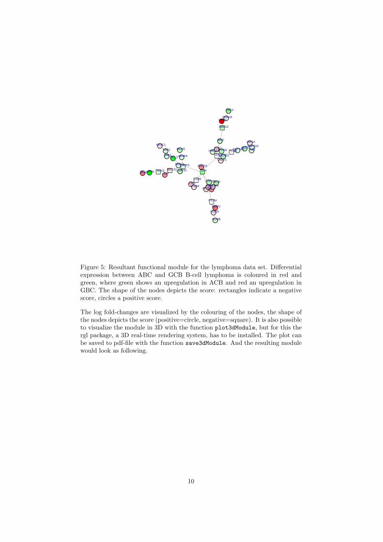
Figure 5: Resultant functional module for the lymphoma data set. Differentialexpression between ABC and GCB B-cell lymphoma is coloured in red andgreen, where green shows an upregulation in ACB and red an upregulation inGBC. The shape of the nodes depicts the score: rectangles indicate a negativescore, circles a positive score.

The log fold-changes are visualized by the colouring of the nodes, the shape ofthe nodes depicts the score (positive=circle, negative=square). It is also possibleto visualize the module in 3D with the function plot3dModule, but for this thergl package, a 3D real-time rendering system, has to be installed. The plot canbe saved to pdf-file with the function save3dModule. And the resulting modulewould look as following.

10

HIF1A

SET ANP32A

APEX1

DNTTIP2

PCNA

CALD1

MYC

RAC2

SMAD4

SMAD2

LMO2

HMGA1

CDC2

PTPN2

CDK7

PTK2

ACTN1CCNE1

ITGAV

ITGB5

MMP2

NUMB

NR3C1

BAG1

BAK1

MCM2

BCL2

AKAP8

BCL6

IRF4

JUP

TRAF2

BIRC2

CASP10

CASP3

RGS16

LYN

SRP72

PIK3R1

PTPN6

LCK

BCR

CD36

ITGA6CD9

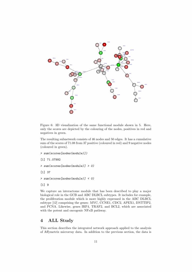
Figure 6: 3D visualization of the same functional module shown in 5. Here,only the scores are depicted by the colouring of the nodes, positives in red andnegatives in green.

The resulting subnetwork consists of 46 nodes and 50 edges. It has a cumulativesum of the scores of 71.08 from 37 positive (coloured in red) and 9 negative nodes(coloured in green).

> sum(scores[nodes(module)])

[1] 71.07992

> sum(scores[nodes(module)] > 0)

[1] 37

> sum(scores[nodes(module)] < 0)

[1] 9

We capture an interactome module that has been described to play a majorbiological role in the GCB and ABC DLBCL subtypes. It includes for example,the proliferation module which is more highly expressed in the ABC DLBCLsubtype [12] comprising the genes: MYC, CCNE1, CDC2, APEX1, DNTTIP2,and PCNA. Likewise, genes IRF4, TRAF2, and BCL2, which are associatedwith the potent and oncogenic NFκB pathway.

4 ALL Study

This section describes the integrated network approach applied to the analysisof Affymetrix microrray data. In addition to the previous section, the data is

11

analysed for differential expression using the package limma [14]. The resultingmodule can be exported in various formats and for example displayed withCytoscape [13].

4.1 The data

First, we load the microarray data and the human interactome data, which isavailable as a graph object from the BioNet package. The popular Acute Lym-phoblastic Leukemia (ALL) data set [3] with 128 arrays is used as an example foran Affymetrix single-channel microarray. This data is available in the packageALL [7] as a normalised ExpressionSet.

> library(BioNet)

> library(DLBCL)

> library(ALL)

> data(ALL)

> data(interactome)

The mircroarray data gives results from 128 samples of patients with T-cellALL or B-cell ALL using Affymetrix hgu95av2 arrays. Aim of the integratedanalysis is to capture significant genes in a functional module, all of whichare potentially involved in acute lymphoblastic leukemia and show a significantdifference in expression between the B- and T-cell samples.

> ALL

ExpressionSet (storageMode: lockedEnvironment)

assayData: 12625 features, 128 samples

element names: exprs

protocolData: none

phenoData

sampleNames: 01005 01010 ... LAL4 (128 total)

varLabels: cod diagnosis ... date last seen (21

total)

varMetadata: labelDescription

featureData: none

experimentData: use 'experimentData(object)'

pubMedIds: 14684422 16243790

Annotation: hgu95av2

For the network data we use a data set of literature-curated human protein-protein interactions that have been obtained from HPRD [11]. Altogether theentire network used here comprises 9386 nodes and 36504 edges.

> interactome




In the next step we have to map the Affymetrix identifiers to the protein iden-tifiers of the PPI network. Since several probesets represent one gene, we have

12

to select one or concatenate them into one gene. One possibility is to use theprobeset with the highest variance for each gene. This is accomplished for theExpressionSet with the mapByVar. It also maps the Affymetrix IDs to the iden-tifiers of the network using the chip annotations and network geneIDs, which areunique, and returns the network names in the expression matrix. This reducesthe expression matrix to the genes which are present in the network. Pleasenote that the number of nodes and edges in the network and resulting modulecan slightly vary depending on the version of chip annotation used.

> mapped.eset <- mapByVar(ALL, network = interactome,

+ attr = "geneID")

> mapped.eset[1:5, 1:5]

01005 01010 03002 04006 04007

MAPK3(5595) 7.597323 7.479445 7.567593 7.384684 7.905312

TIE1(7075) 5.046194 4.932537 4.799294 4.922627 4.844565

CYP2C19(1557) 3.900466 4.208155 3.886169 4.206798 3.416923

BLR1(643) 5.903856 6.169024 5.860459 6.116890 5.687997

DUSP1(1843) 8.570990 10.428299 9.616713 9.937155 9.983809

The data set is reduced to 6133 genes. To find out how many genes are containedin the human interactome we calculate the intersect.

> length(intersect(rownames(mapped.eset), nodes(interactome)))

[1] 6133

Since the human interactome contains 6133 genes from the chip we can eitherextract a subnetwork with the method subNetwork or preceed with the wholenetwork. Automatically the negative expectation value is used later when deriv-ing the scores for the nodes without intensity values. We continue by extractingthe subnetwork. Furthermore, we want to identify modules as connected sub-graphs, therefore we use the largest connected component of the network andremove existing self-loops.

> network <- subNetwork(rownames(mapped.eset), interactome)

> network




> network <- largestComp(network)

> network <- rmSelfLoops(network)

> network




So finally we derive a chip-specific network which comprises 5608 nodes and22770 edges.

13


Differential expression In the next step we use limma [14] to analyse differ-ential expression between the B-cell and T-cell groups.

> library(limma)

> design <- model.matrix(~-1 + factor(c(substr(unlist(ALL$BT),

+ 0, 1))))

> colnames(design) <- c("B", "T")

> contrast.matrix <- makeContrasts(B - T, levels = design)

> contrast.matrix

Contrasts

Levels B - T

B 1

T -1

> fit <- lmFit(mapped.eset, design)

> fit2 <- contrasts.fit(fit, contrast.matrix)

> fit2 <- eBayes(fit2)

We get the corresponding p-values and and calculate the scores thereupon.

> pval <- fit2$p.value[, 1]


We have obtained the p-values for each gene for differential expression. Next,the p-values are used to fit the Beta-uniform mixture model to their distribution[5, 10]. The following plot shows the fitted Beta-uniform mixture model in ahistogram of the p-values. The quantile-quantile plot indicates that the BUMmodel fits to the p-value distribution. Although the data shows a slight deviationfrom the expected values, we continue with the fitted parameters.


> fb

Beta-Uniform-Mixture (BUM) model

6133 pvalues fitted

Mixture parameter (lambda): 0.456

shape parameter (a): 0.143

log-likelihood: 11979.3

> dev.new(width = 13, height = 7)

> par(mfrow = c(1, 2))

> hist(fb)

> plot(fb)

14

Histogram of p−values

P−values

Den

sity

0.0 0.2 0.4 0.6 0.8 1.0

05

1015

ππ

0.0 0.2 0.4 0.6 0.8 1.0

0.0

0.2

0.4

0.6

0.8

1.0

QQ−Plot

Estimated p−valueO

bser

ved

p−va

lue

Figure 7: Histogram of p-values, overlayed by the fitted BUM model in red andthe π-upper bound displayed as a blue line. The right plot shows a quantile-quantile plot, in which the estimated p-values from the model fit deviate slightlyfrom the observed p-values.

The nodes of the network are now scored using the fitted BUM model and aFDR of 1e-14. Such a low FDR was chosen to obtain a small module, whichcan be visualized.

> scores <- scoreNodes(network = network, fb = fb,

+ fdr = 1e-14)

In the next step the network with the scores and edges is written to file and theheinz algorithm is used to calculate the maximum-scoring subnetwork.

> writeHeinzEdges(network = network, file = "ALL_edges_001",


[1] TRUE

> writeHeinzNodes(network = network, file = "ALL_nodes_001",

+ node.scores = scores)

[1] TRUE

4.4 Calculation of the maximum-scoring subnetwork

In the following the heinz algorithm is started using the heinz.py python script.A new implementation Heinz v2.0 is also available at https://software.cwi.nl/software/heinz , with slightly different and additional options. This startsthe integer linear programming optimization and calculates the maximum-scoringsubnetwork using CPLEX.

The command is: ”heinz.py -e ALL edges 001.txt -n ALL nodes 001.txt -N True-E False” or runHeinz on a linux machine with CPLEX installed.

15

The output is precalculated in ALL_nodes_001.txt.0.hnz andALL_edges_001.txt.0.hnz in the R BioNet directory, subdirectory extdata.The output is loaded as a graph with the following commands:


> module <- readHeinzGraph(node.file = file.path(datadir,

+ "ALL_nodes_001.txt.0.hnz"), network = network)

Attributes are added to the module, to depict the difference in expression andthe score later.

> nodeDataDefaults(module, attr = "diff") <- ""

> nodeData(module, n = nodes(module), attr = "diff") <- fit2$coefficients[nodes(module),

+ 1]

> nodeDataDefaults(module, attr = "score") <- ""

> nodeData(module, n = nodes(module), attr = "score") <- scores[nodes(module)]

> nodeData(module)[1]

$`BTK(695)`

$`BTK(695)`$geneID

[1] "695"

$`BTK(695)`$geneSymbol

[1] "BTK"

$`BTK(695)`$diff

[1] 0.919985

$`BTK(695)`$score

[1] -8.866502

We save the module as XGMML file and look at it with the software Cytoscape[13], colouring the node by their ”diff” attribute and changing the node shapeaccording to the ”score”.

> saveNetwork(module, file = "ALL_module", type = "XGMML")

[1] "...adding nodes"

[1] "...adding edges"

[1] "...writing to file"

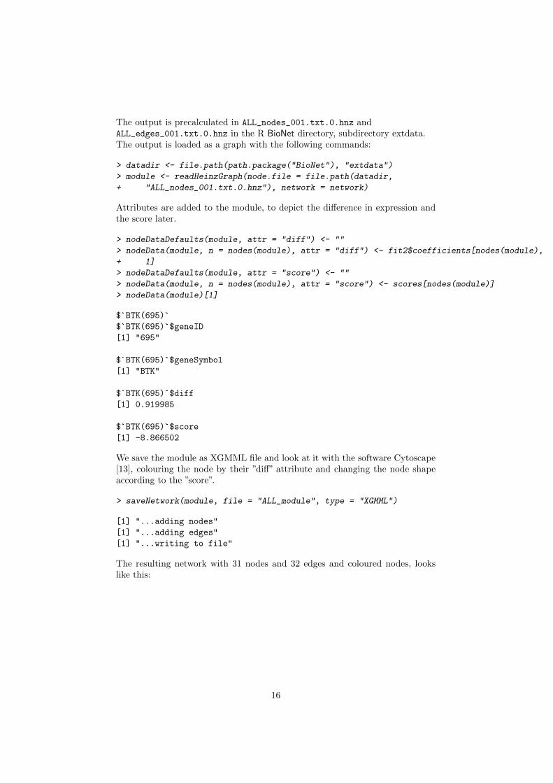
The resulting network with 31 nodes and 32 edges and coloured nodes, lookslike this:

16

Figure 8: Resultant module visualized in Cytoscape. Significantly upregu-lated genes are coloured in red, genes that show significant downregulation arecoloured in green, for the contrast B vs. T cells. The score of the nodes is shownby the shape of the nodes, circles indicate a positive score, diamonds a negativescore.

The module comprises several parts, one part showing a high upregulation in theB-T contrast (CD79A, BLNK, CD19, CD9, CD79B) participates in B cell acti-vation and differentiation and response to stimuli according to their GO anno-tation. While the other large upregulated part is involved in antigen processingand presentation and immune response (HLA-DMA, HLA-DPA1, CD4, HLA-DMB, HLA-DRB5, HLA-DPB1). T cell/leukocyte activating genes (CD3D,CD3G, CD3Z, ENO2, TRAT1, ZAP70) are coloured in green. The lower mid-dle part is involved in negative regulation of apoptosis, developmental processesand programmed cell death. Most of them are involved in overall immune sys-tem processes and as expected, mostly B and T cell specific genes comprise theresulting module, as this contrast was used for the test of differential expression.

5 Consensus modules

To assess the variation inherent in the integrated data, we use a jackknife re-sampling procedure resulting in an ensemble of optimal modules. A consensusapproach summarizes the ensemble into one final module containing maximallyrobust nodes and edges. The resulting consensus module visualizes variable re-gions by assigning support values to nodes and edges. The consensus moduleis calculated using the acute lymphoblastic leukemia data from the previoussection.

17

First, we perform the same steps as explained in 4 and start with the dataobtained up to subsection 4.2. We use the chip-specific network which comprises5608 nodes and 22770 edges and the ALL microarray dataset.


Differential expression We resample the microarrays and calculate p-valuesusing a standard two-sided t-test for the differential expression between the B-cell and T-cell groups. 100 jackknife replicates are created and used to test fordifferential expression.

Depending on the number of resamples the next steps can take a while.

> j.repl <- 100

> resampling.pvals <- list()

> for (i in 1:j.repl) {

+ resampling.result <- resamplingPvalues(exprMat = mapped.eset,

+ groups = factor(c(substr(unlist(ALL$BT),

+ 0, 1))), resampleMat = FALSE, alternative = "two.sided")

+ resampling.pvals[[i]] <- resampling.result$p.values

+ print(i)

+ }

We use the obtained p-values to calculate scores thereupon.


For each jackknife replicate a BUM model is fitted to the p-value distribution,which is used to calculate node scores. The same FDR as before is used.

> fb <- lapply(resampling.pvals, fitBumModel, plot = FALSE,

+ starts = 1)

> resampling.scores <- c()

> for (i in 1:j.repl) {

+ resampling.scores[[i]] <- scoreNodes(network = network,

+ fb = fb[[i]], fdr = 1e-14)

+ }

We create a matrix of scores to calculate the modules. This creates one nodefile as input for the ILP calculation. Alternatively one node file can be createdfor each jackknife resample, which then can be run in parallel on a cluster ormulticore machine. This approach is preferable, due to possibly many jackkniferesamples. For simplification we use the matrix variant here.

> score.mat <- as.data.frame(resampling.scores)

> colnames(score.mat) <- paste("resample", (1:j.repl),

+ sep = "")

The node scores are written to file in the next step. For the edge scores thebinary interactions are written to file with a score of 0.

18

> writeHeinzEdges(network = network, file = "ALL_e_resample",


> writeHeinzNodes(network = network, file = "ALL_n_resample",

+ node.scores = score.mat)

5.3 Calculation of the optimal subnetworks

In the following the heinz algorithm is started using the heinz.py pythonscript. This starts the integer linear programming optimization and calculatesthe maximum-scoring subnetwork using CPLEX. In contrast to previous calcula-tions we define a size the resulting modules should have. We set it with the sizeparameter s to the size of the original module, which was 31. This fixes the sizeof the output modules for a later consensus module calculation.

The command is: ”heinz.py -e ALL e resample.txt -n ALL n resample.txt -NTrue -E False -S 31”

The output is precalculated in ALL_n_resample.txt.0.hnz and ALL_e_resample.txt.0.hnz

in the R BioNet directory, subdirectory extdata. The output is loaded as a listof graphs with the following commands:


> modules <- readHeinzGraph(node.file = file.path(datadir,

+ "ALL_n_resample.txt.0.hnz"), network = network)

5.4 Calculation of the consensus module

We have obtained now 100 modules from the resampled data. These are used tocalculate consensus scores for the nodes and edges of the network and recalcu-late an optimal module. This module, termed consensus module, captures thevariance in the microarray data and depicts the robust solution. Confidence val-ues for the nodes and edges can be visualized by the node size and edge width,allowing to identify stable parts of the module.

We therefore use the modules to calculate consensus scores in the following andrescore the network:

> cons.scores <- consensusScores(modules, network)

> writeHeinz(network = network, file = "ALL_cons",

+ node.scores = cons.scores$N.scores, edge.scores = cons.scores$E.scores)

[1] TRUE

They are run using CPLEX: ”heinz.py -e ALL cons e.txt -n ALL cons n.txt -NTrue -E True -S 31”. Mind to also use the edge scores with -E True.

The results are loaded in R and visualized.


> cons.module <- readHeinzGraph(node.file = file.path(datadir,

+ "ALL_cons_n.txt.0.hnz"), network = network)

19

> cons.edges <- sortedEdgeList(cons.module)

> E.width <- 1 + cons.scores$E.freq[cons.edges] *

+ 10

> N.size <- 1 + cons.scores$N.freq[nodes(cons.module)] *

+ 10

> plotModule(cons.module, edge.width = E.width,

+ vertex.size = N.size, edge.label = cons.scores$E.freq[cons.edges] *

+ 100, edge.label.cex = 0.6)

5024

50

50

4835

48

99100

97

99

93

100

100

29

100100

43

9329100

100100

100

435353

38

4798

100

100

47

43

39

●

●

● ● ●

●●

● ●●

●

●

●

●

●

●

●

●

●

●●

●

●

●

● ●

●

●

●

●

●

BTK

CASP3

CD3DCD3Z

CD4

CD9

CD19

CD44CD74

CD79A

CDKN1A

CTNNA1

CTNNB1

HBEGF

ENO2

CD79B

FOXO1A

HLA−DMB

HLA−DPA1

HLA−DRAIGHM

PLCG2

PRKCQ

PTK2

CD3G TUBA1

ZAP70

BLNK

TRAT1

AJAP1

HLA−DPB1

Figure 9: Resultant consensus module. The size of the nodes and the widthof the edges depict the robustness of this node or edge as calculated from thejackknife replicates.

6 Installation

6.1 The BioNet package

The BioNet package is freely available from Bioconductor athttp://www.bioconductor.org.

6.2 External code to call CPLEX

The algorithm to identify the optimal scoring subnetwork is based on the soft-ware dhea (district heating) from Ljubic et al. [9]. The C++ code was extendedin order to generate suboptimal solutions and is controlled over a Python script.

20

The dhea code uses the commercial CPLEX callable library version 9.030 byILOG, Inc. (Sunnyvale,CA). In order to calculate the optimal solution a CPLEXlibrary is needed. The other routines, the dhea code and heinz.py Python script(current version 1.63) are publicly available for academic and research purposeswithin the heinz (heaviest induced subgraph) package of the open source libraryLiSA (http://www.planet-lisa.net). The dhea code has to be included inthe same folder as heinz.py, in order to call the routine by the Python code. Tocalculate the maximum-scoring subnetwork without an available CPLEX licensea heuristic is included in the BioNet package, see runFastHeinz.The new version of Heinz v2.0 is available at https://software.cwi.

nl/software/heinz.

References

[1] Vince Carey, Li Long, and R. Gentleman. RBGL: An interface tothe BOOST graph library, 2009. URL http://CRAN.R-project.org/

package=RBGL. R package version 1.20.0.

[2] Vincent J Carey, Jeff Gentry, Elizabeth Whalen, and Robert Gentleman.Network structures and algorithms in Bioconductor. Bioinformatics, 21(1):135–136, Jan 2005.

[3] Sabina Chiaretti, Xiaochun Li, Robert Gentleman, Antonella Vitale, MarcoVignetti, Franco Mandelli, Jerome Ritz, and Robin Foa. Gene expressionprofile of adult t-cell acute lymphocytic leukemia identifies distinct subsetsof patients with different response to therapy and survival. Blood, 103(7):2771–2778, Apr 2004.

[4] Gabor Csardi and Tamas Nepusz. The igraph software package for complexnetwork research. InterJournal, Complex Systems:1695, 2006. URL http:

//igraph.sf.net.

[5] Marcus T Dittrich, Gunnar W Klau, Andreas Rosenwald, Thomas Dan-dekar, and Tobias Muller. Identifying functional modules in protein-proteininteraction networks: an integrated exact approach. Bioinformatics, 24(13):i223–i231, Jul 2008.

[6] R. Gentleman, Elizabeth Whalen, W. Huber, and S. Falcon. graph: A pack-age to handle graph data structures, 2009. URL http://CRAN.R-project.

org/package=graph. R package version 1.22.2.

[7] Wolfgang Huber and Robert Gentleman. estrogen: 2x2 factorial designexercise for the Bioconductor short course, 2006. R package version 1.8.2.

[8] Trey Ideker, Owen Ozier, Benno Schwikowski, and Andrew F Siegel. Dis-covering regulatory and signalling circuits in molecular interaction net-works. Bioinformatics, 18 Suppl 1:S233–S240, 2002.

[9] I. Ljubic, R. Weiskircher, U. Pferschy, G. W. Klau, P. Mutzel, and M. Fis-chetti. An Algorithmic Framework for the Exact Solution of the Prize-Collecting Steiner Tree Problem. Math. Program., Ser. B, 105(2-3):427–449, 2006.

21

[10] Stan Pounds and Stephan W Morris. Estimating the occurrence of falsepositives and false negatives in microarray studies by approximating andpartitioning the empirical distribution of p-values. Bioinformatics, 19(10):1236–1242, Jul 2003.

[11] T. S Keshava Prasad, Kumaran Kandasamy, and Akhilesh Pandey. Humanprotein reference database and human proteinpedia as discovery tools forsystems biology. Methods Mol Biol, 577:67–79, 2009.

[12] Andreas Rosenwald, George Wright, Wing C Chan, Joseph M Connors,Elias Campo, Richard I Fisher, Randy D Gascoyne, H. Konrad Muller-Hermelink, Erlend B Smeland, Jena M Giltnane, Elaine M Hurt, HongZhao, Lauren Averett, Liming Yang, Wyndham H Wilson, Elaine S Jaffe,Richard Simon, Richard D Klausner, John Powell, Patricia L Duffey,Dan L Longo, Timothy C Greiner, Dennis D Weisenburger, Warren GSanger, Bhavana J Dave, James C Lynch, Julie Vose, James O Ar-mitage, Emilio Montserrat, Armando Lopez-Guillermo, Thomas M Gro-gan, Thomas P Miller, Michel LeBlanc, German Ott, Stein Kvaloy, JanDelabie, Harald Holte, Peter Krajci, Trond Stokke, Louis M Staudt, andLymphoma/Leukemia Molecular Profiling Project. The use of molecularprofiling to predict survival after chemotherapy for diffuse large-B-cell lym-phoma. N Engl J Med, 346(25):1937–1947, Jun 2002.

[13] Paul Shannon, Andrew Markiel, Owen Ozier, Nitin S Baliga, Jonathan TWang, Daniel Ramage, Nada Amin, Benno Schwikowski, and Trey Ideker.Cytoscape: a software environment for integrated models of biomolecularinteraction networks. Genome Res, 13(11):2498–2504, Nov 2003.

[14] Gordon K. Smyth. Limma: linear models for microarray data. In R. Gen-tleman, V. Carey, S. Dudoit, and W. Huber R. Irizarry, editors, Bioin-formatics and Computational Biology Solutions using R and Bioconductor,pages 397–420. Springer, New York, 2005.

22

bionet tutorial - bioconductor · october 30, 2018 abstract the rst part of this tutorial exempli...

Documents