biomolecular computing – combinatorial algorithms and
TRANSCRIPT
Giuditta Franco
Biomolecular Computing –Combinatorial Algorithms andLaboratory Experiments
Ph.D. Thesis
21st April 2006
Universita degli Studi di Verona
Dipartimento di Informatica

Advisor:prof. Vincenzo Manca
Series N◦: TD-04-06
Universita di VeronaDipartimento di InformaticaStrada le Grazie 15, 37134 VeronaItaly

A mia madre


Contents
Table of Contents . . . . . . . . . . . . . . . . . . . . . . . . . . . . . . . . . . . . . . . . . . . . . . . . . . V
Preface . . . . . . . . . . . . . . . . . . . . . . . . . . . . . . . . . . . . . . . . . . . . . . . . . . . . . . . . . . . . VII
1 Introduction . . . . . . . . . . . . . . . . . . . . . . . . . . . . . . . . . . . . . . . . . . . . . . . . . . . 11.1 Molecular computing . . . . . . . . . . . . . . . . . . . . . . . . . . . . . . . . . . . . . . . . 3
1.1.1 Unconventional computational models . . . . . . . . . . . . . . . . . . . 51.1.2 Why choosing DNA to compute? . . . . . . . . . . . . . . . . . . . . . . . . 7
1.2 DNA computing . . . . . . . . . . . . . . . . . . . . . . . . . . . . . . . . . . . . . . . . . . . . . 81.2.1 Theory and experimentation . . . . . . . . . . . . . . . . . . . . . . . . . . . . 111.2.2 Attacking NP-complete problems . . . . . . . . . . . . . . . . . . . . . . . . 141.2.3 Emerging trends . . . . . . . . . . . . . . . . . . . . . . . . . . . . . . . . . . . . . . 16
1.3 This thesis . . . . . . . . . . . . . . . . . . . . . . . . . . . . . . . . . . . . . . . . . . . . . . . . . . 171.4 Conclusive notes . . . . . . . . . . . . . . . . . . . . . . . . . . . . . . . . . . . . . . . . . . . . 20
2 Floating Strings . . . . . . . . . . . . . . . . . . . . . . . . . . . . . . . . . . . . . . . . . . . . . . . 232.1 DNA structure . . . . . . . . . . . . . . . . . . . . . . . . . . . . . . . . . . . . . . . . . . . . . . 242.2 String duplication algorithms . . . . . . . . . . . . . . . . . . . . . . . . . . . . . . . . . 272.3 DNA pairing . . . . . . . . . . . . . . . . . . . . . . . . . . . . . . . . . . . . . . . . . . . . . . . . 332.4 DNA-like computations . . . . . . . . . . . . . . . . . . . . . . . . . . . . . . . . . . . . . . 382.5 Membrane systems . . . . . . . . . . . . . . . . . . . . . . . . . . . . . . . . . . . . . . . . . . 43
2.5.1 Some variants . . . . . . . . . . . . . . . . . . . . . . . . . . . . . . . . . . . . . . . . . 452.5.2 Applications . . . . . . . . . . . . . . . . . . . . . . . . . . . . . . . . . . . . . . . . . . 49
3 Cross Pairing PCR . . . . . . . . . . . . . . . . . . . . . . . . . . . . . . . . . . . . . . . . . . . . 573.1 PCR . . . . . . . . . . . . . . . . . . . . . . . . . . . . . . . . . . . . . . . . . . . . . . . . . . . . . . . 58
3.1.1 PCR variants . . . . . . . . . . . . . . . . . . . . . . . . . . . . . . . . . . . . . . . . . 653.2 Splicing rules . . . . . . . . . . . . . . . . . . . . . . . . . . . . . . . . . . . . . . . . . . . . . . . 683.3 XPCR procedure . . . . . . . . . . . . . . . . . . . . . . . . . . . . . . . . . . . . . . . . . . . . 703.4 An extraction algorithm . . . . . . . . . . . . . . . . . . . . . . . . . . . . . . . . . . . . . . 733.5 DNA involution codes . . . . . . . . . . . . . . . . . . . . . . . . . . . . . . . . . . . . . . . . 75
VI Contents
4 On Generating Libraries by XPCR . . . . . . . . . . . . . . . . . . . . . . . . . . . . 794.1 A generation algorithm . . . . . . . . . . . . . . . . . . . . . . . . . . . . . . . . . . . . . . . 814.2 Combinatorial properties . . . . . . . . . . . . . . . . . . . . . . . . . . . . . . . . . . . . . 824.3 A couple of special strands . . . . . . . . . . . . . . . . . . . . . . . . . . . . . . . . . . . 854.4 Generalized generation algorithm . . . . . . . . . . . . . . . . . . . . . . . . . . . . . . 884.5 Advantages of XPCR generation . . . . . . . . . . . . . . . . . . . . . . . . . . . . . . 93
5 Applications of XPCR . . . . . . . . . . . . . . . . . . . . . . . . . . . . . . . . . . . . . . . . . 975.1 The satisfiability problem (SAT) . . . . . . . . . . . . . . . . . . . . . . . . . . . . . . 985.2 Restriction enzymes . . . . . . . . . . . . . . . . . . . . . . . . . . . . . . . . . . . . . . . . . 1005.3 An enzyme-based algorithm to solve SAT . . . . . . . . . . . . . . . . . . . . . . . 101
5.3.1 Generation step . . . . . . . . . . . . . . . . . . . . . . . . . . . . . . . . . . . . . . . 1035.3.2 Extraction step . . . . . . . . . . . . . . . . . . . . . . . . . . . . . . . . . . . . . . . 105
5.4 A mutagenesis algorithm . . . . . . . . . . . . . . . . . . . . . . . . . . . . . . . . . . . . . 1075.5 Past and future applications . . . . . . . . . . . . . . . . . . . . . . . . . . . . . . . . . . 109
5.5.1 Support to cancer research . . . . . . . . . . . . . . . . . . . . . . . . . . . . . 1115.5.2 Ethical aspects . . . . . . . . . . . . . . . . . . . . . . . . . . . . . . . . . . . . . . . . 112
6 Laboratory Experiments . . . . . . . . . . . . . . . . . . . . . . . . . . . . . . . . . . . . . . . 1156.1 Melting temperature . . . . . . . . . . . . . . . . . . . . . . . . . . . . . . . . . . . . . . . . . 1166.2 In a laboratory . . . . . . . . . . . . . . . . . . . . . . . . . . . . . . . . . . . . . . . . . . . . . . 118
6.2.1 PCR protocol . . . . . . . . . . . . . . . . . . . . . . . . . . . . . . . . . . . . . . . . . 1196.2.2 Gel-electrophoresis . . . . . . . . . . . . . . . . . . . . . . . . . . . . . . . . . . . . 122
6.3 XPCR-based extractions . . . . . . . . . . . . . . . . . . . . . . . . . . . . . . . . . . . . . 1256.4 XPCR-based generation . . . . . . . . . . . . . . . . . . . . . . . . . . . . . . . . . . . . . . 127
6.4.1 Recombination witnesses . . . . . . . . . . . . . . . . . . . . . . . . . . . . . . . 1306.5 XPCR-based mutagenesis . . . . . . . . . . . . . . . . . . . . . . . . . . . . . . . . . . . . 132
7 A Model for DNA Self-Assembly . . . . . . . . . . . . . . . . . . . . . . . . . . . . . . 1357.1 Forbidding-enforcing systems . . . . . . . . . . . . . . . . . . . . . . . . . . . . . . . . . 1367.2 The model: graphs from paths . . . . . . . . . . . . . . . . . . . . . . . . . . . . . . . . 1387.3 Forbidding-enforcing graphs . . . . . . . . . . . . . . . . . . . . . . . . . . . . . . . . . . 141
7.3.1 Graphs for DNA structures . . . . . . . . . . . . . . . . . . . . . . . . . . . . . 142
8 Conclusions and Ongoing Research . . . . . . . . . . . . . . . . . . . . . . . . . . . . 1478.1 DNA silencing . . . . . . . . . . . . . . . . . . . . . . . . . . . . . . . . . . . . . . . . . . . . . . 1508.2 On modelling knee injuries by membrane systems . . . . . . . . . . . . . . . . 152
8.2.1 The process . . . . . . . . . . . . . . . . . . . . . . . . . . . . . . . . . . . . . . . . . . 1548.2.2 Experiment . . . . . . . . . . . . . . . . . . . . . . . . . . . . . . . . . . . . . . . . . . . 1568.2.3 A membrane system . . . . . . . . . . . . . . . . . . . . . . . . . . . . . . . . . . . 158
References . . . . . . . . . . . . . . . . . . . . . . . . . . . . . . . . . . . . . . . . . . . . . . . . . . . . . . . . . 161
Acknowledgments . . . . . . . . . . . . . . . . . . . . . . . . . . . . . . . . . . . . . . . . . . . . . . . . . 173
Sommario . . . . . . . . . . . . . . . . . . . . . . . . . . . . . . . . . . . . . . . . . . . . . . . . . . . . . . . . . 17710.1 Problemi e risultati principali . . . . . . . . . . . . . . . . . . . . . . . . . . . . . . . . . 17910.2 Conclusione . . . . . . . . . . . . . . . . . . . . . . . . . . . . . . . . . . . . . . . . . . . . . . . . . 181
Preface
I first heard of molecular computing at the Department of Biology in Pisa, whereI was hanging out, as an undergraduate student of mathematics, with the firm in-tent to learn a certain programming language. I ended up in a lecture of ProfessorVincenzo Manca (who would later become the supervisor of this thesis), and itwas amazing. Researchers were trying to compute in a novel manner, by process-ing information stored in biomolecules according to innovative paradigms, and to“decipher” computations taking place in nature, by observing biological processesfrom a mathematical perspective. A speculative investigation which genuinely com-bines an interest in living beings with the logic behind the abstract perfection ofmathematics, seemed to me extremely attractive. Moreover, the chance to analyzean alternative concept of computation inspired by nature stimulated my curiosityand my imagination. I have not learned that programming language as yet, but af-ter that lecture I continued to attend the whole class, thus starting my enthusiasticstudies in molecular computing and (theoretical) computer science.
This thesis collects most of my research in molecular computing, according tothe chronological order in which it was conceived, while some additional contri-butions are briefly mentioned along the way. The original content of the thesishas been almost entirely published or submitted for publication, and the papersare respectively listed at the end of the chapters that are based on them. Thereader may also find some more recent ideas in Chapter 8, where work in progressis outlined. Most of the results presented arose from collaboration, mainly withmy advisor and his group, but also with people coming from other departments(computer science, mathematics) and from medical schools. For this reason, theacademic we is often preferred to I.
After an introduction in Chapter 1, which offers a condensed overview of theliterature and current trends in molecular computing, with more details in DNAcomputing, together with a presentation of the problems faced in this dissertation,we proceed through three research phases.
Firstly, we ponder why the DNA molecule is assembled as a pair of filaments ofopposite directions exhibiting Watson-Crick complementarity between the corre-sponding bases. What differences would we find, if it were differently structured?Why antiparallelism? Why just four bases? Since we did not find any biologicalaccount for these facts, we looked for an explanation in informational or computa-

VIII Preface
tional terms. An algorithmic analysis of DNA molecular features addresses thesequestions in Chapter 2, and the double stranded DNA structure turns out to bea requirement necessary for the efficiency of the DNA autoduplicating process.A DNA-like duplication algorithm is then extended to universal computations ondouble strings, while a general presentation of membrane systems concludes thechapter. In particular, in membrane computing, a different computational perspec-tive is suggested, that shifts the focus of attention from the evolution of individualobjects to that of a population of objects. The same approach is useful for lab-oratory DNA computations, where one is generally unable to know exactly whathappens to an arbitrary single strand, but it is possible to manipulate a poolof strands, in such a way that after a computation the pool satisfies a certainproperty, as was the case in the experiments reported in Chapter 6.
Secondly, we perform computations with DNA strings in vitro (in contrast toin vivo) both in theoretical (dry) and experimental (wet) contexts. A variant of thePolymerase Chain Reaction, which is perhaps the most widely applied technique inmolecular biology, is introduced as an implementation basis for generation, extrac-tion and mutagenesis procedures. Novel applications, which improve methods to befound in the literature, are presented by means of bioalgorithms that are based onpolymerase action. Theoretical investigations of a specifically guided generation ofDNA libraries are described, as well as laboratory experiments that validate thosealgorithms. Namely, Chapter 4 showcases a simple example of how mathematicalresults may be motivated from, and prove significant for, an experiment in DNAcomputing.
Finally, we broaden our interest from linear self-assembly of double strings toa three-dimensional self-assembly process. Recently this has been the subject ofextensive studies, since the construction of complex structures at the nano scale isthe key challenge at the core of the emerging discipline of Nanoscience. The possibleoutcomes of the self-assembly process must comply with constraints which arisefrom the physical and chemical properties of DNA, and are described in Chapter 7by a set of forbidding and enforcing rules. Forbidding-enforcing systems are analternative device to generate formal languages that was inspired by chemicalprocesses. This device was put to work to simulate DNA-based computations, andafterwards it was introduced to the context of membrane computing. A variantof forbidding-enforcing systems for graphs is proposed here, modelling the DNAself-assembly process and suggesting new research directions in graph theory.
The three phases outlined above are put forth as more or less selfcontainedstages of a research journey, the main results being found in the middle one. Ihope this arrangement makes for a smoother access by those readers who areinterested in just some parts of this dissertation.
Verona, March 31, 2006
1
Introduction
Computer Science is no more about computersthan astronomy is about telescopes.
Edsger Wybe Dijkstra
Computer science is a pretty reductive name to connote the discipline of infor-mation processing, unless we take our mind away from the machines populatingour everyday life and we think of a ‘computer’ just as an apparatus performingsome kind of computation. More precisely, the attention should be focused on thenature of computation more than on the device performing computation. On theother hand, concepts as information, processes, computations, algorithms are sowide and pervasive that some context seems necessary to put any problem relatingto the nature of computation in the right focus.
Information is one of the fundamental building blocks of the universe, and acomputation is a process that transforms information. This looks like a nice pre-sentation, but it says all and nothing. I prefer to introduce the idea of informationas an analogue of the well known notion of energy1. Much like energy is expressedby the motion of matter and by its changing of form, analogously information ismanifested by the transformation of data, that is, by the change from a repre-sentation in a certain kind of data into another one, within another kind of data.To give a more evident analogy, as energy also is the potential to perform work,so information also is the potential to rule the performance of work. In fact, theperforming of work releases energy according to some constraints, and informationestablishes such constraints to select some work processes out of all the possibleones.
If we think of information as being numerical, statistical, qualitative, quan-titative, symbolic, biological, genetic, linguistic, artistic, then we realize how theidea of information is deeply related to concepts of action, communication, data,form, representation1. Although it is an abstract entity, we cannot study its ‘being
1 This idea is proposed and widely discussed along with interesting examples in Chap-ter 6 of the book: V. Manca, Metodi Informazionali, Bollati Boringhieri, 2003.

2 1 Introduction
processed’ without taking the physical supports on which it is represented intoaccount. That is to say, we may keep track of the transformation, transmission,conservation, deterioration of information expressed by data represented, for ex-ample, on paper, electronic or magnetic supports, or molecules. Hence, we need toconsider the structure as well as the location in space and the temporal life of suchsupports. Note that this approach assumes the discrete and quantitative nature ofdata, underlying digital information (in contrast to analogical information, givenby continuous measures that are then approximated by discrete quantities).
The processing of information requires a strategy of systematical data trans-formation by means of basic operations called computations. The definition ofsuch basic operations depends on the type of data to which they apply, as wellas on their organization within physical supports. An algorithm is such a strategy(more intuitively, in [9] it is characterized by P. Arrighi as “a recipe to solve amathematical problem”), and a computational process is the procedure composedof the computations running onto a specific system. We shall use the words ‘algo-rithm’ and ‘computational procedure’ indifferently, because it will be clear fromthe context which system do they run on and what kinds of computations do (bio-)algorithms refer to.
The concepts of algorithm and computation emerged even earlier than the ideaof mathematical proof, which was introduced by the ancient Greeks along with theaxiomatic deductive method of Euclidean geometry. Those concepts may alreadybe found in the first documents of ancient civilizations, connected to problems ofmeasurements of land plots or altars2. The Ahmes book (XVII century AC) is arich example, where the algorithmic solutions of eighty problems were elaboratedby Egyptian mathematicians, and comparable works can be retrieved from ancientArabic, Indian and Chinese civilizations3. The idea of computational model, onthe contrary, was only introduced in the past century, along with the Mathemat-ical Logic of the thirties [227], where the concept of computable function arosefrom the computational equivalence of such diverse formalisms as the λ-calculusby Alonzo Church and the computing machine by Alan M. Turing. The von Neu-mann architecture was influenced by Turing (they are computationally equivalentby universality theorem); it is based on the principle of one complex processorthat sequentially performs a single task at any given moment, and has dominatedcomputing technology for the past sixty years. Recently, however, researchers havebegun exploring alternative computational systems inspired by biology and basedon entirely different principles.
Nowadays, are new theories of computation worth the effort of their creation?There are several reasons to believe the effort has been well spent [130]. First ofall, it is important to determine the conditions under which the present theoryof computation holds. Our present notion of effective computability may be un-necessarily limited, namely if other systems subsume the class of general recursivefunctions [221] and an expanded definition is as useful as the current one for ab-stract problems. A more physically and biologically grounded theory would likely
2 A historical excursus regarding algorithmic theory is given in the book: V. Manca,Note di teoria degli algoritmi, Cooperativa Libraria Universitaria Friulana, 1992.
3 B. L. Van Der Waerden. Geometry and Algebra in Ancient Civilizations, Springer-Verlag, Berlin-Heidelberg, 1983.
1.1 Molecular computing 3
stimulate substantial changes in our understanding of computing and in the designof computers. A theory that could enable the design of better algorithms and ofmolecular computers, would distinctly improve the current situation.
First electronic computers date to the end of the forties, when the molec-ular biology discipline was just born. Since then, there have been speculationsabout exploiting molecules as computational devices [166,233], and first molecularcomputational models have been proposed [133, 65, 45, 15, 16, 46]. As an example,C. Bennett in [15] discusses how RNA could be used as a physical medium to im-plement (reversible) computation, by linking the functioning of RNA polymeraseto the one of a Turing machine, whereas in [16] he gives a description of a hy-pothetical computer, using a macromolecule similar to RNA to store information,and imaginary enzymes to catalyze reactions acting upon the macromolecule. As amatter of fact, computer science and molecular biology have as clear as surprisinganalogies in the data structures on which their fundamental processes are based.Only recently, though, biological computation has become a reality, thanks to re-markable developments both in molecular biology and in genetic engineering, nowproven able to sequence the human genome, to measure enormous quantities ofdata accurately, and to synthesize and manipulate considerable amounts of specificmolecules.
The breakthrough was the experiment which Leonard M. Adleman carried outin November 1994, thereby launching a novel, in vitro approach to solve a Hamil-tonian Path Problem (HPP) instance, over a directed graph with seven vertices,by means of DNA molecules and of standard biomolecular operations [1]. Givena graph and a pair of designated ‘initial’ and ‘final’ vertices, the goal of HPP isto determine whether a path exists, starting from the initial vertex and endingup in the final one, such that it goes through each vertex of the graph exactlyonce. While in conventional computers information is stored as binary numbers insilicon-based memories, in this approach he encoded the information by randomDNA sequences of twenty bases. The computation was performed in a fashion ofbiomolecular reactions, involving procedures such as hybridization, denaturation,ligation, polymerase chain reaction, and a biotin-avidin magnetic beads system.The output of computation, in the form of DNA molecules, was read and printedby means of a standard electrophoresis fluorescence process.
This seminal experiment had a tremendous impact onto the information sciencecommunity, in that it stimulated a huge avalanche of new and exciting research,dealing with both experimental and theoretical issues of computing by molecules.A new philosophy promises to deliver new means for doing computation moreefficiently, in terms of speed, cost, power dissipation, information storage, andsolution quality. Simultaneously, it offers the potential of addressing many moreproblems, also coming from the biological world, than it was previously possible,and the results obtained so far hold prospects for a bright future.
1.1 Molecular computing
In the past fifteen years a fast growing research field called molecular computingemerged in the area of natural computing. The general aim of research in this

4 1 Introduction
area, is to investigate computations underlying natural processes, or taking placein nature, as well as to conceive new computational paradigms and more efficientalgorithms inspired by nature. Significant advances in this area have been madethrough neural networks, evolutionary algorithms, and quantum computing, thatare examples of human-designed computing inspired by nature. In particular, in-formation massively encoded in molecules nowadays can be extensively processedby technologies from molecular biology, and a new type of computation has beenactually initiated (“Most importantly, this research has led already to a deeperand broader understanding of the nature of computation”, G. Rozenberg, [201]).
Biological strings can be obviously seen as strings over an alphabet (having foursymbols in the case of DNA and RNA polymers), and some operations can be quitenaturally imported from formal language theory [202]—which is a mathematicaltheory of strings, essentially. It is not so surprising, though, that when movingto the laboratory reality of a test tube, where strings really float and interact,we lose most of the mathematical assumptions behind formal language theory.For example, the operations of concatenating, reading, and writing strings onmolecules require specific bioalgorithms and ad hoc biotechnological protocols, aswell as other simple operations, like computing their length or ‘taking a string froma set to which it belongs’. Universal computations of the Turing machine can besimulated at a molecular level (for a recent reference see [174]), in a different fashionthough, where selective cutting, pasting (concatenating), pairing and elongatingstrings are natural operations, while the moving of a reader along a string is morespecific and limited to the action of some enzymes—quite unlike what happens ona tape. Moreover, nature does not ‘compute’ just by sequence rewriting but also bycrossing-over, annealing, insertion-deletion and so on. Nonetheless, while readingand writing are not so obvious, parallelism of computations and compactness ofinformation storage are given for free by nature, and the limits to miniaturizationof silicon technology do not exist anymore. Interestingly enough, novel algorithmsare thus designed in order to make molecular computations robust, that are basedon different, appropriate kinds of operations.
As it emerged from discussions with Vincenzo Manca, an important new featurewhich is common to molecular and quantum computations is that they can beobserved and captured only at certain moments. In both cases indeed, one cannotcontrol step by step what is the exact effect of the operations, and one alters thesystem when observing the result. The sound way to account for what happensbetween the moment of preparing an initial system and the moment of measuringit is to think of the complex components of the state as amplitudes, or proportions(rather than probabilities). As an example, a quantum coin can be in a state ofboth head and tail, in some proportions, simultaneously, until one measures it.This feature is just a means of exploring several possibilities simultaneously [9].The case of DNA operations is interesting as well, they are performed on pools,identified with multisets (sets with a multiplicity associated to their elements)of strings over a given alphabet, but we do not really know which are the exactmultisets before and/or after the application of the operations. In fact, to thispurpose we would need to estimate how many copies of each different moleculeare present at any given moment, and how many of them are modified by theoperation as expected, but this claim is not realistic at all, because we are only

1.1 Molecular computing 5
able to observe macro-states of the pool. Realistically speaking, the output pool isa mixed population of ‘solutions’ and ‘other outcomes’, and no theory of molecularcomputation may presume a single unambiguous, exact result of computation.
Despite this kind of approximation, that we could say microscopic nondetermi-nation of the computation, bioalgorithms driving system behaviours can be writtensuch that the final pool of molecules contains the desired solution [150]. This factuncovers a different perspective of computing: one does not care what happens ex-actly to each sequence in each test tube, but one knows that an operation appliedto certain data yields a pool of data satisfying a certain property. The individualnondeterminism is left unaffected, while population properties are controlled bymacro-steps. This approach seems to be a best way to really manipulate compu-tations in nature, rather than trying to fit the (mysterious) natural processes intopre-conceived, exact computational models.
Nevertheless, no new model may escape the comparison with traditional com-putational models; and a significant research stream in molecular computing aimedat molecular implementation of classical models of computation. For example,molecular implementation of Turing machines was considered in the articles [15]and [198], where detailed molecular encodings of the transition table of a Turingmachine are given, and further Turing machines with few instructions can be foundin [195]. Molecular implementations of linear context-free grammars [59], Post sys-tems [63], cellular automata [242], and push-down automata [39] were discussed aswell. Maybe more interestingly, new computational models were introduced andextensively investigated, such as aqueous computing, forbidding-enforcing comput-ing, and membrane computing.
1.1.1 Unconventional computational models
Tom Head, in [101], introduced a framework of aqueous computing as a kind ofmolecular computing free from code design, while the first aqueous computationto be completed was done in Leiden by operating on plasmids [104]. This worksolved the problem of computing the cardinal number of a maximal independentsubset of the vertex set of a graph, by dealing with the same instance faced in [175].In general, aqueous computing requires both water-soluble molecules on which aset of identifiable locations can be specified, and a technology for making localalterations and for detecting the condition of molecules. A vast number of suchmolecules are dissolved in the ‘water’ (i.e., an appropriate fluid where the chosenmolecules are soluble), and the initial state of each of the specified locations takesa bit value. At this point one can ‘write on the molecules’ by altering such bitvalues: the first phase of computation always consists of a sequence of writingsteps. After suitable separations and unifications of pools of molecules, the resultof the computation is ‘read’ from the state of the molecules. More recent examplesof aqueous computing can be found in [102,225].
Andrzej Ehrenfeucht, Hendrik Jan Hoogeboom, Grzegorz Rozenberg and Nikevan Vugt, in [55], introduced the forbidding-enforcing model that is inspired bychemical reactions, where the presence of a certain group of molecules impliesthe presence of other specific molecules eventually, while ‘conflicting’ reactantsmay not be present simultaneously in the system. This model was novel both

6 1 Introduction
from the viewpoint of molecular systems and from that of computation theory, inthat it suggested a new way to compute a whole family of outcomes, all of whichobey the forbidding and enforcing constraints of the system [58]. The result ofan evolving computation of the system can be, for example, a possibly infinitefamily of languages, or the result of interactions between DNA molecules, butthe computational model is not restricted to operations on strings. Indeed, it wasapplied to membrane computations [37], and also to describe some processes ofDNA self-assembly as computations on graphs [74]. More details about this modelare reported in Section 7.1.
Gheorghe Paun, in [178], introduced the first class of discrete models directlyinspired by living cell structure and functioning. They were named P-systems, aftertheir “inventor”, or membrane systems, because of their hierarchically arrangedstructure of membranes, all embedded inside one, outermost “skin membrane”.This compartmentalization in regions delimited by (and one by one associated to)membranes is a crucial point of the model, to compute in a parallel and distributedway. Each membrane region is associated to a multiset of objects which evolve ac-cording to the set of rules relating to that region. The evolution of (each regionof) the system is performed in a maximally parallel way, that is by nondetermin-istically assigning objects to the rules until no further assignment is possible. Allcompartments of the system evolve synchronously (a common clock is assumed forall membranes), therefore there are two layers of parallelism: between the objectsinside the membranes and between the membranes inside the system. A com-putation starts from an initial configuration of the system, that is defined by acell-structure with objects and a set of rules for each compartment, and goes on byapplying rules as described above, until it reaches a configuration where no morerules apply to the existing objects. The move from a configuration of the systemto a next one is called transition, and a computation is a sequence of transitions.If such a sequence is finite, then it is a halting computation and, because of thenondeterminism of rule application, we get a set of results (a language or a set ofnumerical vectors), in a designated (output) membrane.
Membrane computing is thus a framework for distributed parallel processingof multisets inspired by cell biochemistry. In the original definition, three types ofmembrane systems were considered: transition, rewriting and splicing, dependingon the kinds of objects and on the way they are processed. However, the gener-ality of this approach is evident; objects can be symbols, strings, trees, and therules can be associated to the regions, or also to the membranes, and can be ofdifferent type, namely, rules of object transformation or communication (whenobjects move through membranes to adjacent compartments), of membrane cre-ation or dissolution. Models inspired by the way cells are organized to form tissuewere considered as well, as a variant of P-systems. More details about membranesystems are recalled in Section 2.5.
From a theoretical point of view, membrane computing is an extension of molec-ular computing, where objects represent molecules and rules represent molecularcomputations. Since the computation proceeds in a distributed, parallel manner,membrane systems model well both in vivo and in vitro molecular computations(“Decentralization, random choices, nondeterminism, loose control, asynchroniza-tion, promoting/inhibiting, control paths are key-words of the ‘natural computing’,

1.1 Molecular computing 7
of the manner the cell preserves its integrity, its life, but they are still long termgoals for computer science in silico, a challenge for computability in general.” Gh.Paun, in [181]).
Usually, biomolecular computations are implemented in vitro, hence outsideof living cells, by manipulating DNA and related molecules moving around testtubes or compartments of a membrane system. However, some attempts in vivohave been made; for example, boolean circuits were simulated in living cells byconducting in vivo evolution of RNA switches by a self-cleaving ribozyme [232],and, more recently, finite-state automata based on a framework which employs theprotein-synthesis mechanism of Escherichia Coli have been implemented in [173].Regarding molecular computations in vitro, although there are interesting exam-ples of RNA-based computing [137, 61], the DNA support has been more widelyexploited and investigated.
1.1.2 Why choosing DNA to compute?
First of all, one should wonder why molecular computing is focused on biomoleculesrather than other kinds of molecules existing in nature4. Certainly, strings areuseful to encode discrete data and to compute, and natural polymers are especiallyapt to this purpose. Besides, by having strings as data structures, one can apply(or at least relate molecular computing to) all the results from formal languagetheory, which underlies the theory of computation, and from information theory.In Section 1.1 the main features of biological strings are described. The reason whyour attention is focused on strings coming from living cells is that, in this case,nature also gives us plenty of tools (enzymes, recognizing systems, interactingsystems) to process them and to perform molecular computations. Moreover, thebiomolecular world is well known, and it may prove more interesting because of thenumerous applications to medicine, thus fascinating us because of the influence on,and the proximity to, our own life. It turns out that, in this context, DNA polymersare usually favorite objects of interest.
As matter of fact, DNA evolved to become the primary carrier of genetic infor-mation thanks to its extraordinary chemical properties. The same properties alsomake DNA an excellent system for the study of biomolecular algorithms, includ-ing self-assembly, which is a wonderful example of self-organization process [155].Intra-molecular interactions between DNA single strings can be precisely predictedby Watson-Crick base pairing, and these interactions are structurally understoodat the atomic level. Given the diversity of DNA sequences, one can easily engineera large number of pairs of DNA molecules that associate with each other in spec-ified sequences and in a well-defined fashion. This property is not common withother molecular systems. Small organic and inorganic molecular pairs can interactwith each other with specificity and in well-defined structures, but the number ofsuch pairs is limited and their chemistry varies greatly. Protein molecules, such asantibody-antigen pairs, have great diversity and high specificity [11]. However, itis extremely difficult, if not impossible, to predict how do proteins interact witheach other. Moreover, DNA sequences have the advantage to be stable (a dry DNAmolecule has a stability of about one billion of years!) and easily manipulable even4 The author thanks her advisor for this stimulating question.
8 1 Introduction
at room temperature, they have convenient modifying enzymes and automatedchemistry, they may be heated without suffering any damage and, when paired,they form an externally readable code [5].
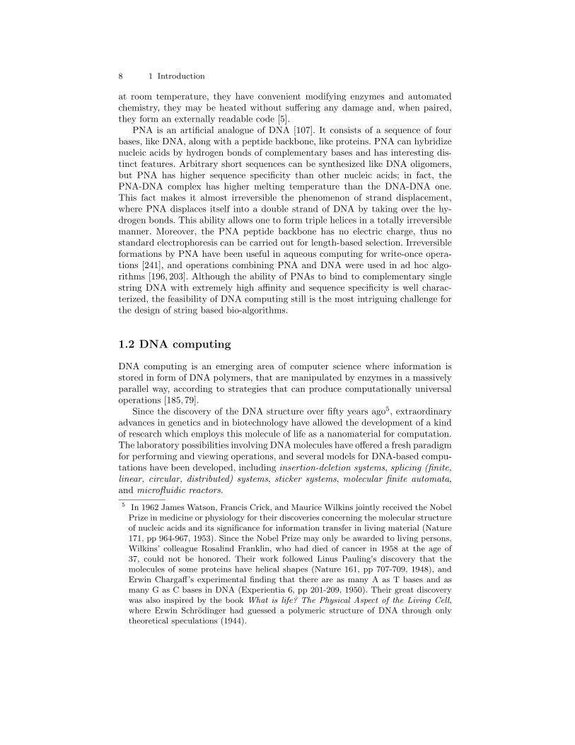
PNA is an artificial analogue of DNA [107]. It consists of a sequence of fourbases, like DNA, along with a peptide backbone, like proteins. PNA can hybridizenucleic acids by hydrogen bonds of complementary bases and has interesting dis-tinct features. Arbitrary short sequences can be synthesized like DNA oligomers,but PNA has higher sequence specificity than other nucleic acids; in fact, thePNA-DNA complex has higher melting temperature than the DNA-DNA one.This fact makes it almost irreversible the phenomenon of strand displacement,where PNA displaces itself into a double strand of DNA by taking over the hy-drogen bonds. This ability allows one to form triple helices in a totally irreversiblemanner. Moreover, the PNA peptide backbone has no electric charge, thus nostandard electrophoresis can be carried out for length-based selection. Irreversibleformations by PNA have been useful in aqueous computing for write-once opera-tions [241], and operations combining PNA and DNA were used in ad hoc algo-rithms [196, 203]. Although the ability of PNAs to bind to complementary singlestring DNA with extremely high affinity and sequence specificity is well charac-terized, the feasibility of DNA computing still is the most intriguing challenge forthe design of string based bio-algorithms.
1.2 DNA computing
DNA computing is an emerging area of computer science where information isstored in form of DNA polymers, that are manipulated by enzymes in a massivelyparallel way, according to strategies that can produce computationally universaloperations [185,79].
Since the discovery of the DNA structure over fifty years ago5, extraordinaryadvances in genetics and in biotechnology have allowed the development of a kindof research which employs this molecule of life as a nanomaterial for computation.The laboratory possibilities involving DNA molecules have offered a fresh paradigmfor performing and viewing operations, and several models for DNA-based compu-tations have been developed, including insertion-deletion systems, splicing (finite,linear, circular, distributed) systems, sticker systems, molecular finite automata,and microfluidic reactors.5 In 1962 James Watson, Francis Crick, and Maurice Wilkins jointly received the Nobel
Prize in medicine or physiology for their discoveries concerning the molecular structureof nucleic acids and its significance for information transfer in living material (Nature171, pp 964-967, 1953). Since the Nobel Prize may only be awarded to living persons,Wilkins’ colleague Rosalind Franklin, who had died of cancer in 1958 at the age of37, could not be honored. Their work followed Linus Pauling’s discovery that themolecules of some proteins have helical shapes (Nature 161, pp 707-709, 1948), andErwin Chargaff’s experimental finding that there are as many A as T bases and asmany G as C bases in DNA (Experientia 6, pp 201-209, 1950). Their great discoverywas also inspired by the book What is life? The Physical Aspect of the Living Cell,where Erwin Schrodinger had guessed a polymeric structure of DNA through onlytheoretical speculations (1944).
1.2 DNA computing 9
Insertion-deletion systems were first considered by Gheorghe Paun in [177],and then by other authors, for example in [126]. They are computational systemsbased on context-sensitive insertion and deletion of symbols or strings. They havebeen studied from a formal language theory viewpoint, initially with motivationsfrom linguistics and then with inspirations from genetics, since both insertingand deleting may be easily seen as operations performed by enzyme action or bymismatching annealing [185]. An experimental counterpart of such systems couldbe the programmed mutagenesis, implemented in [131]. This is a sequence-specificrewriting of DNA molecules, where copies of template molecules are produced thatfeature engineered mutations at sequence-specific locations.
The first achievement by mathematical analysis of biochemical operations ofDNA recombination had resulted in the formulation of splicing systems, introducedby Tom Head in [97]. Roughly speaking, a splicing operation is a new type ofstring rewriting rule on double DNA sequences, inspired by a phenomenon of DNArecombination in vivo which involves restriction enzymes (recognizing a specific‘site’ and cutting the sequence at that position) and ligase enzymes (pasting twomolecular fragments by means of their matching ends). Splicing systems wereproposed to model the mathematical (linguistic) properties of DNA recombinantbehaviour, namely in the paper [98] Tom Head suggested the use of circular (cyclic)strands within splicing systems, but a few years later the H systems were consideredas a theoretical model of DNA based-computation.
Extended splicing models have been proposed to the purpose of enhancing thecomputing capability beyond the regularity bound [146], in the hope to achieveTuring machine universal computability [179], while staying within the realisticframework of only allowing finite sets of axioms and of rules. In [184], for exam-ple, Gheorghe Paun, Grzegorz Rozenberg and Arto Salomaa considered splicingrules controlled by a next-rule mapping, like in programmed grammars, and foundan abstract model where the splicing rules are themselves modified from step tostep by means of pointwise mutations of the one-symbol insertion-deletion type.Although extended H systems with regular sets of rules characterize the familyof recursively enumerable (RE) languages, yet as long as they have finite sets ofaxioms and of rules their language generating power cannot exceed the family ofregular languages [147]. Quite surprising in this context is the result by MatteoCavaliere, Natasa Jonoska and Peter Leupold, who obtained universal computa-tion by using finite splicing systems equipped with simple observing and acceptingdevices that consist of finite state automata [38]. More details on simple H systemsmay be found in Section 3.2.
Splicing systems were extended to tree structures in [208], and the languagefamily generated by tree splicing systems was shown to be the family of context-freelanguages. Universal models based on H systems with permitting and forbiddingcontext, inspired by in vivo promoters and inhibitors respectively, were investigatedas well [179]. Finally, splicing membrane systems concerning membrane computingwith string objects and splicing rules were investigated [178], and structures thatare similar to parallel communicating grammar systems were obtained in the formof distributed H systems [47,49], where different parts of the model work indepen-dently and the computation result is deduced from the partial results produced in

10 1 Introduction
such parts. With three context-free components, one can characterize the familyof RE languages.
Regular simple sticker systems have been introduced in [124], where primitivebalanced and fair computations of dominoes were discussed. They were then ex-tended into bidirectional sticker systems, where the prolongation in both directionswas conceived, so that they appeared in a general form with dominoes of arbitraryshapes corresponding to DNA molecules [182]. A classification of sticker systemsas well as their generative capacity was thoroughly investigated in [185].
The automata counterpart of the sticker systems are the Watson-Crick au-tomata, introduced in [80], which handle data structures different to the cus-tomary ones. Their objects are in fact double strings assumed to be paired bythe Watson-Crick complementarity relation, rather than linear, one-dimensionalstrings of symbols, and automata that (at least in their initial definition) scaneach of the two strands separately, albeit in a correlated manner. Although theseautomata exploit a DNA-like support for computation, they perform operationsin the standard sequential way, thus lacking the massive parallelism of DNA com-putation.
A recent breakthrough in the approaches to using DNA as an autonomousmachine for computation was achieved in Israel by a group leaded by EhudShapiro [14]. The combination of a type of restriction endonuclease enzyme calledFokI, used as a tool to change states in a finite state automaton, and a rather smartencoding of states and symbols, yielded a successful in vitro implementation oftwo-state DNA automata. Three main ideas were exploited: use of the restrictionendonuclease FokI, encoding (state, symbol) pairs with both sequence and lengthof the segment, and consideration of accepting sequences for final readout. Sucha DNA automaton changes its states and reads the input without outside media-tion, solely by the use of the enzyme. The authors demonstrated simulations forseveral automata with two states. In the implementation, a total amount of 1012
automata sharing the same software (‘transition molecules’) run independentlyand in parallel on inputs in 120 µl solution, at room temperature at a combinedrate of 109 transitions per second with a transition fidelity greater than 99.8 %.However, this method encounters certain limitations when trying to extend it tomore than two states.
Takashi Yokomori, Yasubumi Sakakibara and Satoshi Kobayashi, in [244], haveproposed a theoretical framework, using a length-encoding technique, that presentsno limitations in implementing nondeterministic finite automata with any num-ber of states. In order to encode each state transition with DNA single strands,no special design technique for the encoding is required, but only the length ofeach sequence involved is important. A computation process is accomplished byself-assembly of encoded complementary strands, and the acceptance of an in-put string is determined by the detection of a completely hybridized DNA doublestrand. Experiments in vitro to implement such a model are reported in [135].Finite automata ranging from two to six states were tested under several inputs,and in particular one six-state finite automaton executed its computation, recog-nizing a given input string. The result is definitely noteworthy, though a gener-alization would probably present experimental difficulties. Indeed, the imprecisebiotechniques (like extraction by affinity purification) employed in the implemen-

1.2 DNA computing 11
tation risk to jeopardize the result, and so also do the repeated patterns in DNAsequences, that produce several unexpected, redundant PCR products (materialdissipation).
Finally, a (theoretical) way to implement general computing devices with un-bounded memory was suggested in [39], where one may find a procedure to im-plement automata with unbounded stack memory, push-down automata, by usingcircular DNA molecules and a type of restriction enzyme called PsrI. The sameideas are there extended to show a way to implement push-down automata withtwo stacks (i.e., universal computing devices), by using two circular moleculesglued together by means of a DX molecule, and a class of restriction enzymes.
The research related to micro-flow reactors has started in [89] and has the goalto improve the programmability of DNA-based computers. Novel clockable mi-croreactors are connected in various ways, and DNA strings flow through channelswhere programmable operations can be performed [228]. Compared to test tubes,microfluidics may have certain advantages, such as small amount of solution, highreaction speeds, and the possibility of easy automation [229].
1.2.1 Theory and experimentation
Here I would like to portray how the flavour of DNA computing models is changingduring the latest years. Initially they were pretty theoretical, often their imple-mentability was just hypothetical, and usually it was assumed. Models such assticker and splicing systems were widely investigated from a formal language the-ory point of view, and gave us an articulated and abstract understanding of DNAbehaviour. A nice example of this tendency is the paper [152], where the authorsproposed the syntagm ‘DNA computing in info’, as opposed to both in vivo andin vitro, and stressing the fact that they worked in an idealized, mathematicalframework. Actually, they sharply showed that, the abstraction of a DNA com-puting strategy, which was used in several algorithms (for example, in [203]) andexperiments, enables us to compute beyond Turing power, by using devices (finitestate machines) much weaker than Turing machines. Their mathematical assump-tions are comparable to the passage from computers to Turing machines-endowedwith infinite tapes and working an unbounded number of steps, and the claim issimply deduced from the fact that the family of RE languages is not closed undercomplementation.
Autonomous DNA automata and micro-flow reactors, instead, are meant tobecome really implemented as computational devices. The implementation of fi-nite automata with few states is not particularly interesting from the theoreticalviewpoint of formal languages, but it represents a significant advance towards theultimate goal of achieving a biomolecular computer. It has shown that, with propercoding and use of appropriate enzymes, a computational device is possible withoutany outside mediation. This opens up the door to using such devices not just toperform computation, but potentially also in genetics and in medicine.
As it were, the formulation of theoretical models has spurred the production ofactual implementations, favoured by continuous improvements in the underlyingtechnologies; yet no implementation deserves interest per se, rather as long as atheoretical model exists that can provide it with foundations, as well as prove,

12 1 Introduction
generalize, or just confirm the results it yields. The highly and genuinely inter-disciplinary field of molecular computing is an evident example where theory andpractice grow up together, just because of their interchange and complementar-ity, in tight duality, as facets of the same coin [5]. Namely, self-assembly of DNAmolecules has recently inspired models that combine theoretical and experimentalaspects. Let us start with a few basic principles of DNA self-assembly.
Two complementary molecules of single-stranded DNA have paired bases thatbind to each other and form the well known double helix structure (duplex). Alinear molecule can fold on itself, in that case it forms a hairpin structure, which isprovoked by autonomous hybridization between two complementary subsequencesof the single stranded molecule (for a picture see Figure 3.13, which is takenfrom [73]). Two molecules of double-stranded DNA (duplexes) can further gluetogether if they have complementary single-stranded overhangs (sticky ends)—fora picture see left side of Figure 7.7 coming from [73]. A 3-arm branched moleculeconsists of three duplex arms arranged around a center point (for a picture seeFigure 7.8, which is taken from [74]), while a double crossover molecule (DX)consists of two adjacent duplexes with two points of strand exchange. Formallanguage characterizations of the computing power of molecular structures (withmore attention to hairpin formations) are explored in [186].
Erik Winfree pioneered a thorough investigation on models of self-assembly [239,235]. The physical system considered from a formal language theory viewpointin [239] was the following. We synthesize several sequences of DNA, mix themtogether in solution, heat it up and slowly cool it down, allowing complexes ofDNA to form chemically or enzymatically ligate adjacent strands. By denatur-ing the DNA again, in the solution we find new single stranded DNA sequencesformed by a concatenation of the initial ones. In other words, some languagesof {A, T,C,G}? are generated by such a self-assembly system. The result provedin [239] is that the family obtained by admitting i) only duplex formations is thefamily of regular languages, ii) only duplex, hairpins, and 3-armed junctions is thefamily of context-free languages, iii) only duplex and DX molecules is the family ofrecursively enumerable languages. Moreover, in [235], Erik Winfree proposed theDNA block model, and together with Tony Eng and Grzegorz Rozenberg provedthat the self-assembly of DNA tiles (also called two-dimensional self-assembly) iscapable of simulating a universal Turing machine [237], by showing that the foursticky ends in a DX molecule can be considered as four sides of a Wang tile6. Bytiling the plane with Wang tiles one can simulate the dynamics of one-dimensionalcellular automata, whence that of a Turing machine.
From the experimental viewpoint, nanoscale guided constructions of complexstructures are one of the key challenges involving science and technology in thetwenty-first century. One of the first synthesized DNA molecules with a struc-ture deviant from the standard double helix is the stable four-junction molecule(now known as J1), that was designed in the late 80’s in the laboratory of N.C.
6 A Wang tile is a planar unit square whose edges are colored. A tile set is a finite setof Wang tiles. A configuration consists of tiles which are placed on a two-dimensionalinfinite grid. A tiling is a configuration in which two juxtaposed tiles have the samecolor on their common border. These concepts were introduced in: H. Wang. Provingtheorems by pattern recognition II. Bell Systems Technical Journal, 40: 1-41, 1961.
1.2 DNA computing 13
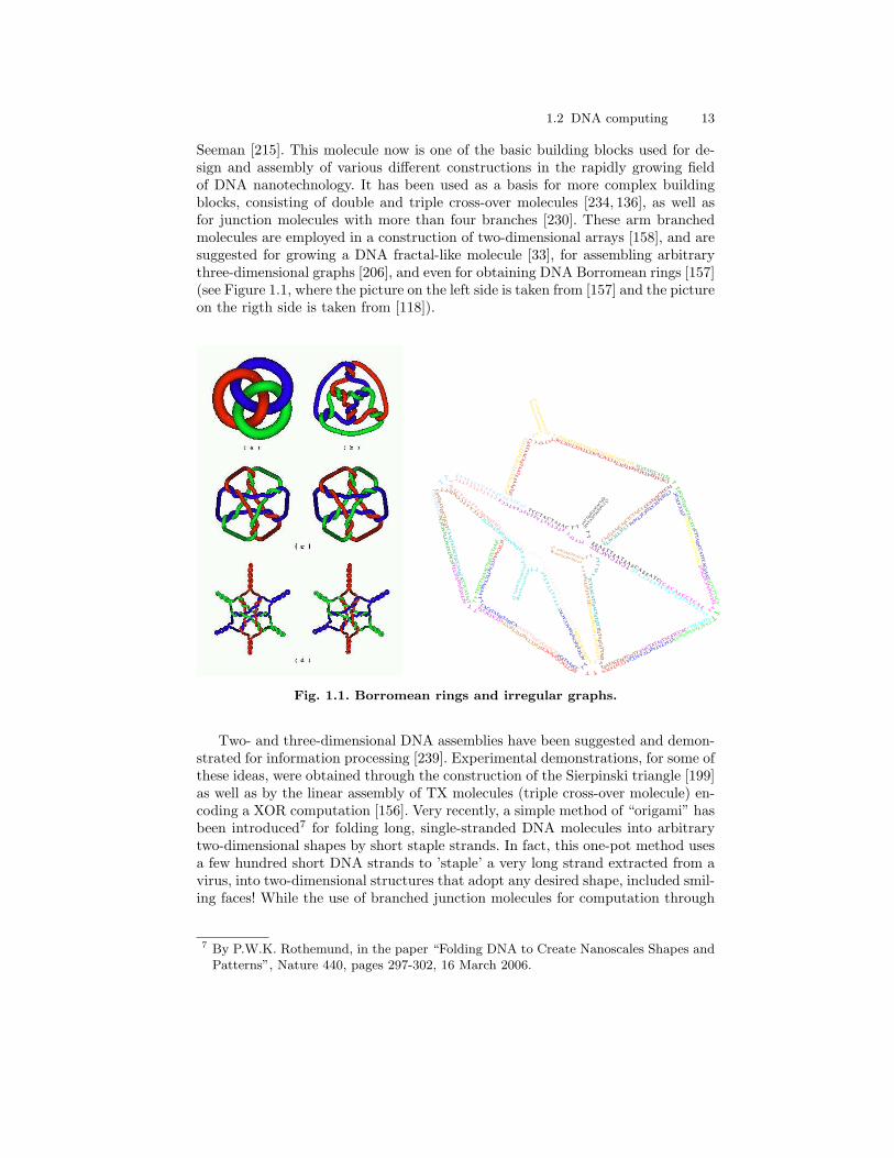
Seeman [215]. This molecule now is one of the basic building blocks used for de-sign and assembly of various different constructions in the rapidly growing fieldof DNA nanotechnology. It has been used as a basis for more complex buildingblocks, consisting of double and triple cross-over molecules [234, 136], as well asfor junction molecules with more than four branches [230]. These arm branchedmolecules are employed in a construction of two-dimensional arrays [158], and aresuggested for growing a DNA fractal-like molecule [33], for assembling arbitrarythree-dimensional graphs [206], and even for obtaining DNA Borromean rings [157](see Figure 1.1, where the picture on the left side is taken from [157] and the pictureon the rigth side is taken from [118]).
g g A g T T g A T g A g C A g g A T C
CCggTATCA
T C C T A C T A g A C
T T ggCTTACgCgAgACT
gTACTATAgCTCAACCgA
CAACTgAAggTggAT
T
T gC
TCTTA
CA
CTTCAgTTg
T T C
T g A g g C T g T g A g A T C C T g CT C A C A g C C T C A g
T T
TgTA
AgA
gCA
TTC
gTgA
ATg
g C
CTA
AgT
ATg
TA
CTTA
ggCC
ATTC
AC
gAA
T
gTC
CA
TCgC
CTggAgTCATggCgCTagAg
gCgA
TggAC
TAC
ATA
T T
CCATgACTCCAg
CTgCTTCACTg
TT
T
TTC
TAA
CA
TTgAC
TgTgTCC
T
gAgCTATAgTACATCCAC
C T
T A
g T
T A
T g
C
T T AC
TAgC
TTAA
gATC
gTT TT
CgA
TCTT
AA
gCTA
gT
T
CgTAgAATCggCgTACCTC
T
TgATACCggTCggTT
T T
gTA
gCgT
TA
ggCC
TAA
CgC
TAC
Agg
AC
AC
Ag
T T
CA
CTgC
AC
gAgTA
CTC
gTgC
AgT
ggA
CC
AC
TC
T
T
gCgTAAgCC
gAACCTAggCgCAgTCTC
gCgCCTAggTTCTgCCTA
CACgTATggTAggCA
T
T
CC
AgTTC
TAggA
A
CC
TCA
TAgT
TTC
CTA
gAA
CTg
gCTC
TgA
gC
T T
CCATACgTgT TA
CTA
TgA
ggTg
CTT
ggC
AgT
ATA
CTT
gAC
gCA
g
CA
AgTA
TAC
TgCC
AA
gCA
CC
ATC
ATC
gT T g A A C g g A C A T A g C g g A T C g C
CgA
TgATggC
TgCgT
T T
C T C A A
T C CAgTC
g A C T g g A T T g AggAggTACg
T T
C T A T g T C C g T T C
g T C T A g T A g g A g C g A T C C g
T
CAgTgTCgACCAATCgAT T
ggTCgA
CACTg
TT TT
T T
T T T
T TT T
T
T CAT CAAC TCC CAgTgAAgCAgCTCTAgCg
T T
gATCgAgCTCCACAC
TTT
g T gTgg AgCTCgATC
T T
TCA
ATg
TTA
gA
Tg C A
T A A
C T A
A g gA
gTggTC
TT
TT T
CCgATTCTACg
T
gCTC
AgA
g
CACATggATACgAgATgTCTg
gTAgATAggTAAg gTCAgTAgCAgACATC TCgTATCCATgTg
CTACTgACCTTACCTATCTACCgA
TAA
CA
gTAA
Tg gAA
gTgCgCA
CTT
CC
ATT
AC
TgTT
ATC
g
T
CTC
ggAC
gTCTC
ATg
TTTT
CA
TgA
gAC
gTC
CgA
g
T TT TT T
T T T
Fig. 1.1. Borromean rings and irregular graphs.
Two- and three-dimensional DNA assemblies have been suggested and demon-strated for information processing [239]. Experimental demonstrations, for some ofthese ideas, were obtained through the construction of the Sierpinski triangle [199]as well as by the linear assembly of TX molecules (triple cross-over molecule) en-coding a XOR computation [156]. Very recently, a simple method of “origami” hasbeen introduced7 for folding long, single-stranded DNA molecules into arbitrarytwo-dimensional shapes by short staple strands. In fact, this one-pot method usesa few hundred short DNA strands to ’staple’ a very long strand extracted from avirus, into two-dimensional structures that adopt any desired shape, included smil-ing faces! While the use of branched junction molecules for computation through
7 By P.W.K. Rothemund, in the paper “Folding DNA to Create Nanoscales Shapes andPatterns”, Nature 440, pages 297-302, 16 March 2006.
14 1 Introduction
assembling three-dimensional structures was suggested in [118], by demonstratinghow NP-complete problems can be solved by one-step assembly.
1.2.2 Attacking NP-complete problems
One of the first aims of DNA computing was the solving of NP-complete problems,since the massive parallelism and the intrinsic nondeterminism make hard prob-lems tractable, even by using brute force search of solutions (“Molecular computingis justifiably exciting, not least for the alluring prospect of biologically-inspired ma-chines nicely handling NP-complete problems”, T. Kazic, [130]). However, the scal-ing up of the proposed models from toy instances to realistic size remains an openproblem, mainly because of the increasing quantity of DNA strands necessary toencode the initial data. For a graph having the modest size of two hundred vertices,with the Adleman’s strategy one would need “DNA material more than the weightof the Earth” (J. Hartmanis, [96]). For this reason, a few algorithms were proposedwhere the potential solutions are not constructed all at once [169,245,118]. The useof linear duplex molecules to solve NP-complete problems has been surperseded byself-assembly of DNA tiles [199], and more generally by graph self-assembly withjunction molecules [230].
The potential of using DNA molecules for solving computationally hard prob-lems has been extensively investigated both from experimental and from theoreti-cal points of view. The satisfiability problem (SAT) was perhaps the most widelystudied NP-complete problem, tricky theoretical solutions of which can be foundin [112, 245, 154, 203], while experimental solutions of small instances of SAT areproposed in [143, 210,209, 29, 28]. An example of a (theoretical) algorithm in vivosolving SAT can be found in [60], where the boolean circuit is genetically encodedinto DNA which is ideally inserted into a cell, and the cell is programmed to selecta random assignment of variables, test for satisfiability, and display a suitable phe-notype when a satisfying assignment is chosen. A theoretical solution of the roadcoloring problem is presented in [110], while an experimental solution of a smallinstance of the maximal clique problem is reported in [175]. DNA has been usedto solve the knapsack problem [188], and even to implement a simplified versionof poker [240].
After Adleman’s experiment where a solution of an instance of HamiltonianPath Problem was found through DNA strands [1], Lipton showed that the satisfi-ability problem can be solved using essentially the same bio-techniques [143]. Theschema of the Adleman-Lipton extract model consists of two main steps: the com-binatorial generation of the solution space (an initial pool containing DNA strandsencoding all the possible solutions) and the extraction of (the strands encoding)the true solutions. Serious limitations about the quantity of DNA necessary toencode the initial pool of the extract model came up soon [96]. Indeed, it shouldbe enough to guarantee the presence of all possible solutions probabilistically, andthat requires an amount of DNA that is (at least) exponential with the size ofthe instance. Nonetheless, implementation of algorithms solving (toy) combinato-rial problems by the extract model is often exploited to improve generation andextraction methods, that are fundamental operations in biology and in genetic re-combination. On the other hand, various enhancements and alternative approachesto the extract model were suggested.

1.2 DNA computing 15
By way of example, we recall a few algorithms that solve the satisfiabilityproblem by skipping the error prone, laborious and expensive extraction phaseof Adleman’s model. They are based on hairpin formation [210, 209, 94], on alength-based method [109], and on mathematical properties of specific sets of nat-ural numbers [84]. Namely, in [209] hairpin formations represented inconsistentassignments of variables and, once detected, they were destroyed by digestion ofan enzyme. Indeed, each string represented a random assignment, where oppositeboolean values were encoded by complementary substrings. In the length-basedmethod [109], costs of paths (in the weighed graph problem) are encoded by thelength of the oligomers in a proportional way. The advantage is that, after aninitial pool generation and amplification, a simple gel-electrophoresis can separatethe respective DNA duplexes according to their length, which directly decodes thesolutions. In [84] the solution can be uniquely detected by length as well, and thetrick lies in the encoding. This was inspired by [154], and it is based on the nicecharacteristic property of unique-sum sets of natural numbers which is defined asfollows. Set S is unique-sum if the only way of obtaining the sum, say s, of itselements as the sum over a multiset M of elements from S, is by taking each ofthem only once, that is, with M = S. Clauses are encoded by oligomers whoselengths are given by numbers out of a unique-sum set S, so that, when the SATinstance is suitably encoded by a graph, a directed path starting from the initialnode and ending up to the final one represents a solution if, and only if, it is oflength s.
Standard bio-operations were also used to break the Data Encryption Standard(DES) [26], one of the cryptographic systems in widest use previously. Approxi-mately one gram of DNA was needed and, by using robotic arms, the breakingof DES was estimated to take five days. A most significant aside of the analysisfor breaking DES, was that the success is quite likely even with a large number oferrors within the laboratory protocols. The DES breaking problem is still used asan example of application of alternative, biologically inspired methods [6].
The theoretical storage potential of DNA molecules is impressive—one gramof dry DNA occupies a volume of approximately one cubic centimeter and it canstore as much information as approximately 2 1021 bits—when compared to thestorage capacity of current technology, that is approximately 109 bits per gram. Asa matter of fact, DNA molecules approximately have an information density of 2bits per cubic nanometer versus 1 bit per 1012 nm3 for current technology. Yet, theactual capacity of DNA oligonucleotides of a given length to store information inthe globally robust and fault-tolerant way that biology requires, seems to be verydifficult to quantify, or even to estimate [87, 189]. Some studies explored the useof DNA databases for storage of information and for its retrieval by search tech-niques, based on query output by bead separation using a fluorescence activatedcell sorter [13,193]. Test databases of increasing diversity were indeed synthesizedand the construction of an extremely large database was completed. Capacity, datasecurity and specificity of chemical reactions were improved through some experi-ments, for example in [129,40]. The way cells and biomaterials store information isone of the most important and enigmatic problems of our times. Encoding informa-tion in biomolecules for processing in vitro has indeed proven to be a challengingproblem for biomolecular computing. Codeword design and, more generally, data

16 1 Introduction
and information representation in DNA receives an increasing interest, not onlyin order to use biomolecules for computation, but also to shed light on a numberof other problems in areas such as bio-informatics, genetics and microbiology.
1.2.3 Emerging trends
The code word design problem requires producing sets of strands that are likelyto bind in desirable hybridizations, while keeping to a minimum the probabil-ity of erroneous hybridizations (such as cross-hybridization of non-complementarystrands, or formation of secondary structures) that may induce false positive orfalse negative outcomes. It turned out that this is quite a complex problem, andseveral authors have concentrated their studies on developing theoretical codingmodels [106, 114, 113] (see also Section 3.5), computer simulations [86, 214], andeven experimental builds of coding libraries [50]. Usually, word sets are carefullydesigned by using computational and information-theoretic methods, so that theresulting long strands behave well with respect to computation. Direct encodingis, however, not very efficient for the storage or processing of massive amountsof data, because of the enormous implicit cost of DNA synthesis to produce theencoding strands. Indirect and more efficient methods have been proposed in [87]using a set of non-cross-hybridizing DNA molecules as basic elements. Therefore,generation of DNA libraries is a crucial point for the effective production of DNAmemories, and the improvement of generation methods appears highly relevant.
Unfortunately, as a matter of fact, several standard biomolecular protocolsdo not ensure the needed precision for computation. Such techniques have to gothrough several adjustments, and sometimes completely new protocols are neces-sary in order to improve their yield. The solution of a 20-variable SAT problemin [28], for example, was obtained by designing protocols for exquisitely sensitiveand error-resistant separation of a small set of molecules. Hence, the search for aDNA solution of such combinatorial problems, even though not computationallysignificant, may prove fruitful in developing new technologies [111]. An attractivetask nowadays is indeed to characterize models within the scope of the given ex-perimental limitations, and to improve or obtain protocols that are sufficientlyreliable, controllable and predictable. This thesis is mostly along this trend, andit has been exciting to see how the algorithmic analysis of a laboratory proce-dure (namely PCR) may suggest new techniques with useful applications. It isconvenient to formulate methods of molecular biology as biomolecular algorithms,and to study the corresponding molecular processes both from combinatoric andexperimental points of view. The goal is to optimize the efficiency of biomolecu-lar methodologies, not only to improve the reliability of computing, but also formedical and biological applications (“Optimization methods should be viewed notas vehicles for solving a problem, but for proposing a plausible hypothesis to beconfirmed or disconfirmed by further experiments”, R. M. Karp, [127]).
A first step towards a better expertise in DNA manipulation is the under-standing of DNA spontaneous behaviour, namely by means of algorithmic andcomputational analysis of its combinatorial aspects. In this respect, the study ofgene assembly in ciliates is an emergent research line of DNA computing [57,190],discovering and modelling biomolecular processes that take place in living cells.

1.3 This thesis 17
Ciliates are indeed unicellular eukariotes (in particular bi-nucleated cells), namedafter their wisp-like covering of cilia, that perform one of the most complex exam-ples of DNA processing known in any organism, the process of gene assembly.
In their micronucleus, coding regions of DNA (named MDS as ‘macronucleardestined sequences’) are dispersed individually or in groups over the long chromo-some, along which they are separated, and in a sense obscured, by the presence ofnon-coding DNA sequences (named IES as ‘internally eliminated sequences’). Dur-ing sexual reproduction, a macronucleus develops from a micronucleus, througha sophisticated rearrangement mechanism called gene assembly, that excises IESsand orders MDSs in a contiguous manner, to form transcriptionally competentmacronuclear genes. Unscrambling is a particular type of IES removal, where theorder of MDSs in the micronucleus is often radically different from the one in themacronucleus. Discovering which are the assembly strategies of ciliates for a givenmicronuclear gene has been a truly fascinating computational task.
Three types of formal systems were investigated at various levels of abstrac-tion: MDS descriptor, string pointer, and graph pointer reduction systems, andas far as assembly strategies are concerned they turned out to be equivalent [54].Three intramolecular operations (‘ld’, ‘hi’, and ‘dlad’) have been postulated forthe gene assembly process, and they provided a uniform explanation for all knownexperimental data. The gene structure and the operations themselves have beenmodeled at three levels of abstraction, respectively based on permutations, strings,and graphs [56]. The computational power of molecular operations used in geneassembly was previously investigated for a model with intra- and inter-molecularoperations in [139]. Meanwhile, more recently, a model was proposed by DavidPrescott, Andrzej Ehrenfeucht and Grzegorz Rozenberg, that is based on recom-bination of DNA strands guided by templates [191], and its computational powerwas studied as well [48].
I like to conclude this section with words of an expert in the field, NatasaJonoska: “Whatever the results, this area of research has brought together theo-reticians (mathematicians and computer scientists) with experimentalists (molecu-lar biologists an biochemists) to a very successful collaboration. Just the exchangeof fresh ideas and discussions among these communities brings excitement, andquite often, provides a new line of development that could not have been possiblewithout the ‘outsiders’ ” [111] .
1.3 This thesis
Theoretical computer science studies the basic mathematical properties and limitsof computation, such as computability (what can we compute?) and complex-ity (how fast can we compute?), by investigating models of computation, suchas artificially built models and natural phenomena. The research area of molecu-lar computing where this thesis finds its place, lives in this context, with majoradherence to DNA computing.
Molecular computing assumes an abstract notion of molecule as a floating entityin a fluid environment. DNA and membrane computing investigate two differentaspects of this idea or, more precisely, the molecule behaviour is analyzed from two
18 1 Introduction
different observation levels. In the context of DNA computing the molecule is a se-quence with recombinant behaviour, while in the context of membrane computingit is an element which transforms and moves from one compartment to another ofa cellular-like system. Of course, the two aspects are linked, and in nature theycorrespond to the interactions between nucleus and cytoplasm of eukariotic cells.These are complementary perspectives risen from a common inspiration, hencein Chapter 2 we present both of them. A presentation of the DNA structure isindeed followed by an excursus in the membrane computing world together withan application of membrane systems to an immunological process.
We start from the concept of string, by presenting a few investigations about thestructure and the interactions of DNA sequences, which are floating strings. Bilin-earity, complementarity and antiparallelism, typical of the double stranded DNAstructure, are proven in an abstract setting, as efficiency requirements on algo-rithms duplicating ‘mobile strings’. Such duplication of strings is then extended tothe following operations on numbers encoded within strings: duplication, triplica-tion and division by six. These operations guarantee the universality of a DNA-likecomputational system based on rules that have a biotechnological interpretation.
As an attempt at looking at our floating strings from a more abstract level,where the strings lose their own structure and become objects moving betweencompartments, we present membrane systems along with an application to describethe selective recruitment of leukocytes. Actually, membrane computing has beenmainly investigated from two different viewpoints: a model as realistic as possibleaccording to the bio-reality, and a computational device as powerful, elegant andefficient as possible. We worked along the first research line; while the secondone studies the equivalence of P systems to Turing machines, even with reducedmembranes, rules, objects, and explores their potential to solve hard problems.In both cases, the cell biochemical system is redesigned so that it more or lessclosely comes to fulfil the assumptions of the theory of computing, and then it isexamined how well does the theory predict its properties, whether computationalor biological ones.
In our speculations on DNA computations, where theoretical issues were sup-ported by experiments, we realized that a special kind of PCR, that we call CrossPairing PCR or shortly XPCR, can be the basis for new algorithms that solve awide class of DNA extraction and recombination problems. In the middle chapterswe describe such a technique as a biotechnological tool to extract strings contain-ing a given substring from a heterogeneous pool, to generate DNA libraries, andto perform mutagenesis. More in detail, the following three tasks are addressed.
1. Generating a combinatorial library of n-bit binary numbers, encoded in DNAstrands X1, Y1, . . . , Xn, Yn, that is, producing the following pool, containing2n different kinds of strings:
{α1 · · ·αn | αi ∈ {Xi, Yi}, i = 1, . . . , n}.
2. Extracting all those strings from a given pool P which include a given substringγ, that is, obtaining a pool that consists of all the strings out of P that containγ as a substring:
{αγβ | αγβ ∈ P}.

1.3 This thesis 19
3. Performing mutagenesis(X,Y ) on a pool P , which means substituting everyoccurrence of X with an occurrence of Y over the strings of P , that is, turningit into the pool:
{αY β | αXβ ∈ P}.
A few bio-algorithms are proposed, mainly based on polymerase action, thathave noteworthy advantages, such as efficiency and feasibility, with respect tomethods from the literature. Mathematical analysis as well as laboratory experi-ments are presented as supporting our work. This includes a study that is linkedto splicing systems, since XPCR suggests a new way to implement a special kindof recombination that is performed in nature by only few enzymes (about thirty).We designed and implemented an algorithm, that produces a DNA library as thestrictly locally testable language generated by a simple splicing system [164]. Froma theoretical point of view, splicing systems started with this model, while an al-gebraic characterization of this type of splicing systems was obtained in [103], thefirst one for any class of splicing systems. From a biological point of view, thisresult is encouraging, in that it reveals a new capacity to manipulate DNA forgenetic recombination and for the creation of a clone library (that is the startingpoint of any physical mapping effort in order to sequence a genome).
The aforementioned technique was applied to extraction and mutagenesis al-gorithms as well. The first application proves interesting in DNA computing, sincethe extraction operation performed by standard protocols is still problematic anderror prone, while both applications seem to enjoy a biological relevance, for ex-ample in the study of genetic mutations.
The powerful molecular recognition of Watson-Crick complementarity em-ployed in DNA base pairing is also used in various models of biomolecular comput-ing and information processing, to guide the assembly of complex DNA structures.In particular, the process where substructures are spontaneously self-ordered intosuperstructures, that is driven by selective affinity of the substructures, is calledself-assembly. In Chapter 7 we present a particular family of graphs as a theoreti-cal model for the generation of self-assembled DNA forms. The model is a variantof the forbidding-enforcing systems, introduced in [55] as a model of chemical re-actions. We extend this original model to the construction of three-dimensionalstructures and, in particular, we concentrate on structures obtained by DNA self-assembly. On the other hand, as a systematic way of describing classes of graphs,our model may be considered as a starting point for developing new ways to in-vestigate graphs in classical graph theory [74].
In conclusion, the thesis presents both theoretical models of molecular com-putations and novel DNA-based algorithms, corresponding to procedures that arerelevant in biological contexts, and bringing the experimental nature of DNA com-putations to the fore. Namely, specific methods for DNA extraction [72], recombi-nation [77], and mutagenesis have been investigated. A schematic overview follows,that summarizes the contributions of this thesis with respect to the topics outlinedin the previous sections.
In the context of theoretical models, we propose:
20 1 Introduction
• A membrane model for leukocyte selective recruitment [75, 43](collaborationwith Vincenzo Manca, Dep’t of Computer Science, University of Verona, Italy).
• A DNA register machine (collaboration with Maurice Margenstern, LITA, Uni-versity of Metz, France; work inspired by ideas from the paper [76]).
• A few forbidding-enforcing conditions on graphs, that describe self-assemblyprocesses [74, 73] (collaboration with Natasa Jonoska, Dep’t of Mathematics,University of South Florida, USA).
In the context of combinatorial and algorithmic investigations on novel DNAmanipulation methods, we put forth (collaboration with Vincenzo Manca):
• the XPCR technique• an XPCR Extraction Algorithm [72]• an XPCR Mutagenesis Algorithm [150]
and, with more autonomous work of mine:
• an XPCR Recombination Algorithm [77,68]• an Enzyme-based Extraction Algorithm [71]
Finally, we exhibit three experiments which were carried out to test all XPCR-based algorithms (collaboration with Vincenzo Manca, together with Cinzia Gi-agulli and Carlo Laudanna from the Dep’t of Pathology, University of Verona,Italy).
The work of interaction, filtering and translating between the theoretical andthe experimental sides of this research has been the most challenging part. Al-though it is not an ‘orthodox’ computer science research, we think it has beenprecious from a scientific point of view, even exciting, because it highlights anexperimental nature of strings and algorithms.
1.4 Conclusive notes
I should like to cite some relevant and comprehensive reference books where allbasic concepts we are dealing with may be found. A standard and very good text-book on molecular biology is [2], whereas the subjects of DNA computing andmembrane computing can be both approached and deeply understood by read-ing [185,5] and [180,43], respectively. Molecular computing bibliography increasescontinuously, though. Main results and open questions about membrane comput-ing can be found at the website http://psystems.disco.unimib.it, whereas the pro-ceedings of the annual workshop on membrane computing (currently at its sixthedition) are the best ongoing reference for following the vivid research productionin this field (WMC7 will be at Universiteit Leiden, in Leiden, The Netherlands,on July 17-21, 2006). Both the website and the workshop are organized underthe auspices of the European Molecular Computing Consortium, EMCC. A prettygood reference for the most up-to-date results, developments and main interestsof DNA computing all over the world are the proceedings of the annual meetings

1.4 Conclusive notes 21
on DNA-based computers, that started in 1995 and are currently at their eleventhedition (DNA12 will be at Seoul National University, in Seoul, South Korea, onJune 5-9, 2006). Finally, as a reference book on Formal Language Theory it isdefinitely suggested [202], whose notation we adopt in this thesis.
Since one of the goals of this chapter is to introduce molecular computing, andespecially DNA computing, to as many people as possible, a few answers to fre-quent questions I was asked by inexperts in the field follow. With the same intent,those who want to just get a general idea about the subjects of this introductionare advised to consult the following recent, comprehensive articles: [243] is a longand detailed manuscript on molecular computing; [111] is a nice to read surveyof some concepts and developments in DNA computing; [181] is an intuitive andinteresting introduction to membrane computing, about which one may find lotsof details in [183].
While attending conferences on different topics, computer scientists often askedme: What do you mean by ‘complexity’? Can biocomputing relieve us from com-plexity? Isn’t hardness an intrinsic feature of the problem? Why was the biggestSAT solving experiment carried out on 20 variables rather than directly on signif-icantly sized instances? How precise are such computations?
Although there exists no well-founded definition of ‘biocomplexity’, yet this isclearly something different from classical complexity [5]. After an initial attemptto characterize complexity of DNA-based algorithms and protocols in terms of thetraditional concepts of time and space, a notion of complexity seemed necessarythat could capture other aspects of the physical-chemical reality (volume, temper-ature, amount of DNA and nucleotides) wherein biocomputation takes place [88].A possible definition considers the number of different sequences as ‘space’ com-plexity of a test tube of DNA [62], and the ‘time’ complexity of an algorithm as thenumber of ‘biosteps’ (elementary physical or chemical steps, such as the changingof temperature or the action of an enzyme), among which the extraction opera-tions should be definitely considered the dominant ones. I should like to concludethat a little bit of experience and common sense is fairly important for estimatingcomplexity of bio-algorithms.
A problem is called ‘hard’ when it belongs to the class NP, i.e., that of problemssolvable in polynomial time by a nondeterministic Turing machine. Intuitivelyspeaking, a problem S is NP-complete if every problem belonging to NP canbe ‘translated’ in polynomial time into an instance of S. Hardness seems to bean intrinsic feature of a problem as far as we consider the Turing machine asreference model for every possible computation. Whenever we go to explore analternative model, and especially a different way to compute, the hardness mightdisappear, and we would thus be ‘saved from complexity’. This seems not to bethe case with DNA computing though—as mentioned earlier, the initial hopesabout solving NP problems have actually fallen beyond, while a different trendhas came up, whereby combinatorial problems are just an expedient to understandnatural phenomena and to improve our ability to manipulate biomolecules. Ina DNA computing experiment, significantly sized problems still require a gooddeal of tasks that cannot be addressed by current technology and bioalgorithms.Research in DNA computing is pushing the barrier of problem size by suggestingand improving methods that may scale up better, but the achievement of solving
22 1 Introduction
realistic problems is really far away. At the present infancy stage, techniques arejust gradually analyzed, tested, and improved.
Although recombinant DNA operations are being automated and robotized,they are still not precise. Many computational steps are based on protocols whichare designed to serve purposes that are particular to molecular biology (henceessentially different from those of DNA computing), and their precision dependstoo much on laboratory conditions that are generally unknown. In each laboratoryprotocol one assumes less than 100% yield, often less than 80%. As yield decreaseswith each additional protocol, it becomes valuable to avail of models and com-putational techniques that require little outside mediation or human interaction.Finding more precise methods, or improving the precision of current techniques,is indeed one of the research trends in DNA computing. In particular, the com-putation error rate is dominated by the error rates of the extract and combinesteps [42].
Errors usually come from two sources: every operation may cause an error, andthe DNA lives a half-life, that is, it decays at a finite rate. If the DNA algorithmexecution takes months, for example, then there is a likely chance that the goodstrands disappear. An error may have huge consequences for biocomputing. Thegoal of bio-algorithms essentially is to keep good strands (encoding a solution ofthe problem) alive and to get rid of bad strands (encoding something else thansolutions). If a good strand is damaged or lost, then the algorithm may fail. Ifbad strands are not removed, there may remain too many bad strands left atthe end of the algorithm execution, and this also may cause failure of the algo-rithm. Right after Adleman’s experiment, the problem of misclassification errorscaused by faulty extracts and strand loss was discussed in detail [62,88,42]. Evenwithout improvements in laboratory techniques, research has shown that solelyalgorithmic methods can reduce error rates significantly [128,200]. In other words,every algorithm for a DNA computer can be mapped to an equivalent one that iscomparatively error-free, admittedly at the cost of increased time and space.
More pragmatic questions used to come from curious friends: How much doesa DNA computing experiment cost? Where does your DNA come from?
The cost of an experiment depends, of course, on the kind of experiment,besides the countries and companies where products are bought from, and it ishard to estimate an average cost. We worked mainly with PCRs and, as a grossindication, a kit of PCR products allowing one to perform 200 PCR reactions of50µl of volume, costs around 200 euros. Actually, the most expensive ingredientturns out to be the polymerase. A good one, able to perform without errors for 1000bases and also auto-correcting, costs up to 1000 euros per vial. The termocycleritself costs between 5000 and 10 000 euros (for real time PCR the cost goes up to20000-30000 euros).
Sequences cost 0.80 euros per base. The kind of DNA that is employed in DNAcomputing experiments usually is synthetic, or “commercially prepared”, includingclones of human proteins or sequences extracted from human genes (that we used,for example, in the experiment reported in Section 6.3). Indeed, the DNA moleculeis known at an atomic level, and it can be perfectly reproduced. The time requiredby current techniques to synthesize a DNA sequence of 100bp in average amountsto approximately ten hours.

2
Floating Strings
Nature uses only the longest threads to weave her patterns,so that each small piece of her fabric
reveals the organization of the entire tapestry.
Richard P. Feynman1
DNA molecules have a structure that satisfies three basic principles: i) they arecomposed of two paired strings, ii) each symbol of a first string corresponds to its‘complementary’ in the second string, iii) these strings are oriented along oppositedirections [85]. These three principles are respectively referred to as: bilinearity,complementarity and antiparallelism. In Section 2.3, we show that they depend ona ‘deep’ logic that is dictated by some informational and computational aspectsof the bilinear duplication algorithm described in Section 2.2. In other words, ifone wants to design an efficient duplication system for strings (finite sequences ofsymbols) represented as mobile polymers (floating in a fluid environment), thenone needs ‘symbol molecules’ asymmetric with respect to the three space directions(as the molecules are from a chemical point of view), and arranged according to thethree principles mentioned above [76]. Moreover, some intrinsic features of DNAmolecules, such as the geometry of the double helix, are proven to be implied bythese principles [148], on which DNA processes are based on.
One of the (first) natural questions to ask about DNA computing concernsits potential to implement arithmetical operations [82]. In Section 2.4 a DNA-like system of rewriting rules on double strings is proposed. This is capable ofuniversal computations, since it performs multiplication by two and by three,and division by six as well. It has been suggested as an extension of the bilinearduplication algorithm, and, it is computationally universal as a consequence of the(universality) results that one can find in [159].
Membrane systems are biologically inspired containers of floating strings. InSection 2.5 a general presentation of membrane systems is given, together with anapplication of them to analyze the immunological process of the selective recruit-
1 The Character of Physical Law, 1965.

24 2 Floating Strings
ment of leukocytes. The approach is that suggested by Gheorghe Paun in [181]: i)one examines a piece of reality, say a particular biological process, ii) one builds aP system modelling it, iii) one writes a program simulating the system2 and per-forms experiments with that program, by turning certain parameters and lookingfor the evolution of the process.
2.1 DNA structure
Nucleotide bases, that are the building blocks of every piece of DNA, are usuallyrepresented by the letters A, C, G, and T, which stand for their chemical names:adenine, cytosine, guanine, and thymine. Yet in 1951 it was clear that the fourbases are not present in the same amount in the organisms, and their relativeproportion widely vary in organisms that are far in the evolution scale. Usuallythough, organisms have all the above four bases, except the virus fago T2 (infectingbacteria) whose DNA has a modified version of the cytosine basis.
Nucleotides have three parts: phosphate group, sugar, and base. The carbonsof sugar are numerated by 1′ through 5′, and those of the base by 1 through 5(for biological details see [85] or [2]). The phosphate group hanging out of the 5′
carbon can join with the hydroxyl group of another nucleotide, at the 3′ carbon,to form a strong (covalent) bond known as phosphodiester bond. As it is displayedin Figure 2.1, which is taken from [85], through this concatenation one obtains onestrand of DNA, i.e., a sequence of nucleotides bonded with phosphodiester bonds.
Fig. 2.1. Concatenation of nucleotides forming DNA strands.
The DNA strands have a natural orientation that is maintained by the con-catenation through the phosphodiester bonds (see right side of Figure 2.1), whilehydrogen bonds anneal two strands with opposite orientation. The A on one strandalways pairs with the T on the other one, and C always pairs with G. Two comple-mentary strands of DNA having opposite orientations thus joint together throughhydrogen bonds, and form a double stranded DNA. The two strands are said tobe Watson-Crick complementary to each other. In the following a double strandedDNA is briefly denoted with dsDNA.
DNA is found within living organisms in the well known double-helix structure,made of two strands wound up around each other. The two strands are antiparallel,2 In my case the program was written by Luca Bianco in [21].

2.1 DNA structure 25
that is, one strand runs 5′ to 3′ while the other one runs 3′ to 5′ (see Figure 2.2,which is taken from [85]). DNA is assembled in the 5′ to 3′ direction and, as aconvention, we read it in the same way. The helix can be virtually of any length;when fully stretched, some DNA molecules are as much as 5 cm long. Nucleotidesproject in towards the axis of the helix, and each one forms hydrogen bonds withthe one directly opposite it, forming base pairs, as displayed in Figure 2.2, whichis taken from [69]. The pairing rules are such that if we read the sequence ofnucleotides on one strand of DNA, we can immediately deduce the complementarysequence on the other strand. They are called the rules of Watson-Crick basepairing, named after the two scientists James Watson and Francis Crick discoveredtheir structural basis in 1951 (for further details see footnote 5 of Chapter 1).
Fig. 2.2. Antiparallel orientation of DNA complementary strands.
One might wonder why adenine never bonds with cytosine, and thymine withguanine. Two purines (A and G) cannot fit within the helix (there is not enoughspace), while two pyrimidines (C and T) cannot get close enough to each other toform hydrogen bonds between them (there is too much space). However, the reason

26 2 Floating Strings
is no longer space, but chemistry: only with the A-T and C-G pairs hydrogen bondscan take place3, and with different strength [2].
Surprisingly enough, a double helix structure with identical angle and lengthproportions can be obtained as a consequence of purely geometrical argumenta-tions as in [148]. The author has investigated the double stranded structure ofDNA molecules in an abstract setting, where the principles on which DNA pro-cesses are based on were formulated in an axiomatic form. A mathematical analysisof interacting ‘monomeric triangles’ yielded to a deeper understanding of the logicinternal to DNA structure, included the formation of major and minor groves inthe double helix (see Figure 2.3, which is taken from [148]). This work was one ofthose cases where an algorithmic and computational investigation of natural pro-cesses can explain molecular structures and phenomena (see Section 1.2.3): “Thepossibility of figuring out mathematical DNA properties, by using general princi-ples and abstract forms, seems to disclose new perspectives in the understandingof this marvelous biological reality” (V. Manca, [148]).
Fig. 2.3. Left side. Form resulting from monomers arranged in a bilinear non-planarstructure. The whole structure is deduced from the values of three angles. Right side.The rotation angle ρ measures the rotation of the single monomer around the axis of thecylinder, the phase angle φ represents the rotation of the cylinder radius correspondingto two monomers that are paired, the torsion angle τ is the angle formed by the ‘head-tailaxis’ of each monomer with the horizontal planes (orthogonal to the cylinder axis).
3 I took this information and an inspiration for the description of the double helix from:R. Mosca, Computational Methods for the Analysis of Genomic Data, PhD thesis,Universita degli Studi di Milano Bicocca, Milan, Italy, 2003.
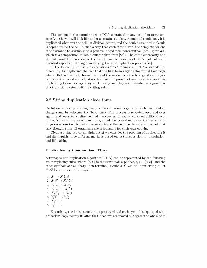
2.2 String duplication algorithms 27
The genome is the complete set of DNA contained in any cell of an organism,specifying how it will look like under a certain set of environmental conditions. It isduplicated whenever the cellular division occurs, and the double stranded moleculeis copied inside the cell in such a way that each strand works as template for oneof the strands to assembly, this process is said ‘semiconservative’ (see Figure 3.1,which is a composition of two pictures taken from [85]). The complementarity andthe antiparallel orientation of the two linear components of DNA molecules areessential aspects of the logic underlying the autoduplication process [76].
In the following we use the expressions ‘DNA strings’ and ‘DNA strands’ in-differently, by neglecting the fact that the first term regards the formal languageswhere DNA is naturally formalized, and the second one the biological and physi-cal context where it actually stays. Next section presents three possible algorithmsduplicating formal strings: they work locally and they are presented as a grammarof a transition system with rewriting rules.
2.2 String duplication algorithms
Evolution works by making many copies of some organisms with few randomchanges and by selecting the ‘best’ ones. The process is repeated over and overagain, and leads to a refinement of the species. In many works on artificial evo-lution, ‘copying’ is always taken for granted, being realized by centralized controlprogram whose task is just to make copies of the genome. In nature it is not thateasy though, since all organisms are responsible for their own copying.
Given a string α over an alphabet ∆ we consider the problem of duplicating itand distinguish three different methods based on: i) transposition, ii) dissolution,and iii) pairing.
Duplication by transposition (TDA)
A transposition duplication algorithm (TDA) can be represented by the followingset of replacing rules, where {a, b} is the (terminal) alphabet, i, j ∈ {a, b}, and theother symbols are auxiliary (non-terminal) symbols. Given an input string α, letSαS′ be an axiom of the system.
1. Si→ XiYiS2. SiS′ → Xi
′ Yi′
3. YiXj → XjYi
4. YiXj′ → Xj
′ Yi
5. XiXj′ → Xi
′j6. YiYj
′ → Yi′j
7. Xi′ → i
8. Yi′ → i
Essentially, the linear structure is preserved and each symbol is equipped witha ‘shadow’ copy nearby it; after that, shadows are moved all together to one side of

28 2 Floating Strings
the structure by keeping their relative positions, so that a shadow copy of the wholeoriginal string is obtained, whence a copy of the original string can be recovered4.
For these replacing rules there is no explicit strategy, but if one wants to ob-tain strings composed of terminal symbols, then the primed symbols have to betransformed into terminals only at the end of the process.
Proposition 2.1. Duplication by transposition performs a number of elementaryrewriting steps that has quadratic order with respect to the length of the initialstring.
Proof. Let n be the length of the string to duplicate. The first step (necessarily)inserts the string between symbols S and S′. Then, the symbol S has to passthrough the first n-1 symbols of the string, and this is done in linear time (n-1steps). For any string and only one time during the process, the third rule must beapplied to eliminate both S and S′. At this point, the first shadow symbol has topass through the last n−1 symbols of the initial string, the second one has to passthrough n − 2 symbols, and so on, the last one does not pass through any othersymbol; therefore n−1+n−2+ . . . 0 = n(n−1)/2 is the number of transpositionsperformed by the algorithm. Finally, 2n steps (one for each symbol of two finalcopies) are necessary to ‘terminalize’ the string.
In conclusion, 1+n− 1+1+n(n− 1)/2+2n steps are necessary (and enough)to duplicate a string of length n, therefore the complexity of TDA is O(n2). ut
Without any change, this algorithm can run in parallel on many strings. Hence,parallel TDA still have a quadratic cost with respect to the length of the longeststring.
We conclude the discussion about TDA with the following example of a rewrit-ing path of the algorithm on the string aba.
1. aba2. SabaS′ (rule 1)3. XaYaSbaS
′ (rule 2)4. XaYaXbYbSaS
′ (rule 2)5. XaYaXbYbXa
′Ya′ (rule 3)
6. XaXbYaYbXa′Ya
′ (rule 4)7. XaXbYaXa
′YbYa′ (rule 5)
4 While referring this dissertation, Gheorghe Paun suggested the following alternativeset of seven (instead of eight) replacing rules. Given an input string α, let SαS′S′′ bean axiom of the system.
1. Si→ iSi′
2. i′ j → j i′
3. i′ S′ → S′ i′
4. i′S′′ → i S′′
5. S S′ → o6. o i→ i o7. o S′′ → λ

2.2 String duplication algorithms 29
8. XaXbXa′YaYbYa
′ (rule 5)9. XaXb
′aYaYbYa′ (rule 6)
10. XaXb′aYaYb
′a (rule 7)11. Xa
′baYaYb′a (rule 6)
12. Xa′baYa
′ba (rule 7)13. abaYa
′ba (rule 8)14. abaaba (rule 9)
Duplication by dissolution (DDA)
Duplication by dissolution was studied in the context of multi-agent systems [153].It dissolves a given string in a solution, while marking the order that any elementhas in the sequence. Then, any element is replicated by a specific agent, and finallythe pieces floating in the solution are recombined (in two copies).
This algorithm is better expressed by rules that transform multisets of strings.Let us fix an alphabet V = T ∪N ∪ {•}, where T is a set of terminal symbols, Na set of numerals, and • a special symbol, and let α, β vary over the strings of T ?,a over the symbols of T , and n,m over N .
The string of T ? that has to be duplicated is put in an initial multiset with aspecial symbol E, standing for an ‘enzyme’, that controls the process. The followingrules yield two copies of the initial string (comma distinguishes the members ofmultisets). Each inference rule replaces a multiset having the form of the premise,with the multiset that is obtained from the conclusion, by assigning to the variablesα, β, a, n,m the same values that were assigned to them in the premise.
• Enzyme binding and marking the first symbol a
E, a α
0 a 1 1 E α(2.1)
• Marking an internal symbol a
α n E a β
α n a n+1 n+1 E β(2.2)
• Releasing the string and the sequence length
α n E
α •, n(2.3)
• Splittingα n n β •
α n • , n β •(2.4)
• Duplicatingn a n+1•
n a n+1 •, n a n+1 •(2.5)
• Recombiningmα n •, n b n+1 •
mα b n+1 •(2.6)
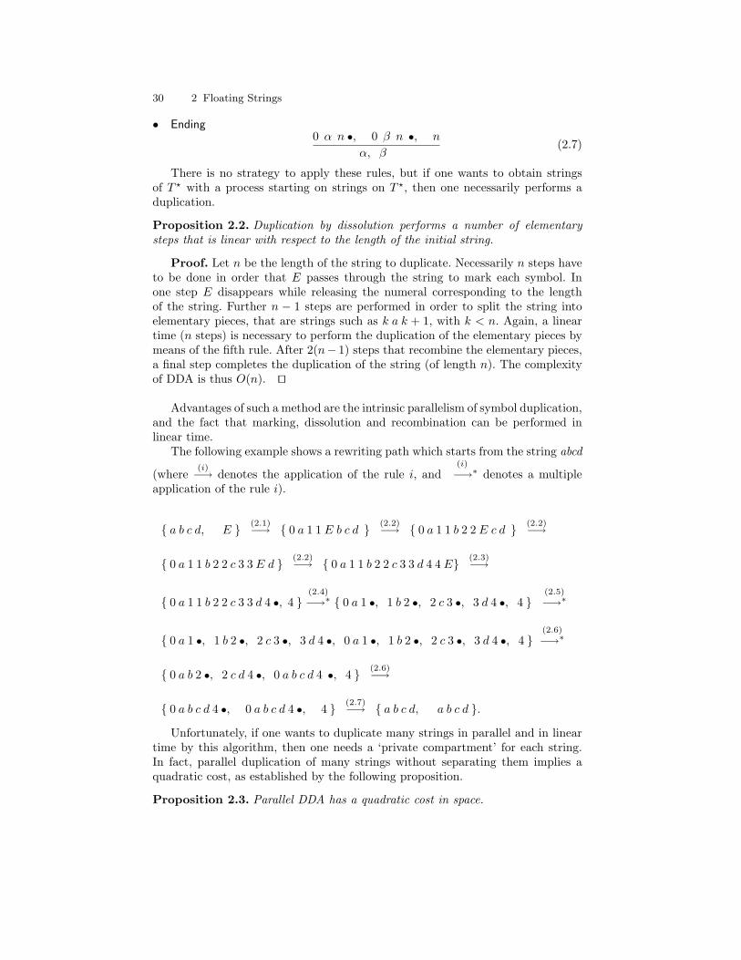
30 2 Floating Strings
• Ending0 α n •, 0 β n •, n
α, β(2.7)
There is no strategy to apply these rules, but if one wants to obtain stringsof T ? with a process starting on strings on T ?, then one necessarily performs aduplication.
Proposition 2.2. Duplication by dissolution performs a number of elementarysteps that is linear with respect to the length of the initial string.
Proof. Let n be the length of the string to duplicate. Necessarily n steps haveto be done in order that E passes through the string to mark each symbol. Inone step E disappears while releasing the numeral corresponding to the lengthof the string. Further n − 1 steps are performed in order to split the string intoelementary pieces, that are strings such as k a k + 1, with k < n. Again, a lineartime (n steps) is necessary to perform the duplication of the elementary pieces bymeans of the fifth rule. After 2(n− 1) steps that recombine the elementary pieces,a final step completes the duplication of the string (of length n). The complexityof DDA is thus O(n). ut
Advantages of such a method are the intrinsic parallelism of symbol duplication,and the fact that marking, dissolution and recombination can be performed inlinear time.
The following example shows a rewriting path which starts from the string abcd
(where(i)−→ denotes the application of the rule i, and
(i)
−→∗ denotes a multipleapplication of the rule i).
{ a b c d, E } (2.1)−→ { 0 a 1 1 E b c d } (2.2)−→ { 0 a 1 1 b 2 2 E c d } (2.2)−→
{ 0 a 1 1 b 2 2 c 3 3 E d } (2.2)−→ { 0 a 1 1 b 2 2 c 3 3 d 4 4 E} (2.3)−→
{ 0 a 1 1 b 2 2 c 3 3 d 4 •, 4 }(2.4)
−→∗ { 0 a 1 •, 1 b 2 •, 2 c 3 •, 3 d 4 •, 4 }(2.5)
−→∗
{ 0 a 1 •, 1 b 2 •, 2 c 3 •, 3 d 4 •, 0 a 1 •, 1 b 2 •, 2 c 3 •, 3 d 4 •, 4 }(2.6)
−→∗
{ 0 a b 2 •, 2 c d 4 •, 0 a b c d 4 •, 4 } (2.6)−→
{ 0 a b c d 4 •, 0 a b c d 4 •, 4 } (2.7)−→ { a b c d, a b c d }.
Unfortunately, if one wants to duplicate many strings in parallel and in lineartime by this algorithm, then one needs a ‘private compartment’ for each string.In fact, parallel duplication of many strings without separating them implies aquadratic cost, as established by the following proposition.
Proposition 2.3. Parallel DDA has a quadratic cost in space.

2.2 String duplication algorithms 31
Proof. In order to duplicate many different strings at the same time, themarking process has to be extended in a such a way that any elementary piece ismarked both with the string to which it belongs and its position inside the string.Since for each of the n symbols of a string we have to store the string itself, thenwe need a O(n2) space capacity of O(n2). ut
Bilinear duplication algorithm (BDA)
If one uses a string as a template and put ‘face-to-face’ to each element a copy ofit, or something that is uniquely associated to it, along a line that goes ‘parallel’to the original one, then one gets an algorithm deeply different from the previousones because it is based on a bilinear structure of strings.
Let V be the alphabet of the string α to duplicate, while • being a meta-symboldescribing the single step of computation. Template driven algorithm or BDA canbe represented by the following rules, where α, β, γ ∈ V ?, λ denotes the emptystring, and the symbol x in V is such that x 6= λ.
1. Starting
α → • αλ
2. Doublingα • x βγ
→ α x • βγ x
3. Separatingα •β→ α, β
A duplication algorithm based on a bilinear structure of strings and determin-istic rewriting rules is thus obtained; in fact, in the last step we have β = α. Inthe case of DNA duplication, in the second step a symbol uniquely associated tox (the complementary) is put ‘face-to-face’ to the template, and finally β resultsto be the Watson Crick complementary string of α.
Proposition 2.4. Parallel BDA has a computational complexity that is linear intime and in space.
Proof. Let n be the length of the string α to duplicate. Apart one initial andone final step, the algorithm performs n doubling steps to copy the symbols of α.Moreover, an amount of space linear with n is occupied during the whole process.ut
Without any change, this algorithm can run in parallel on many strings whilemaintaining a linear complexity.
As an example, we consider a rewriting path of BDA starting from the stringacbdd over the alphabet V = {a, b, c, d} (where −→∗ denotes multiple applicationof a rule).
acbddstarting−→ •acbdd
λ
doubling−→ a•cbdda
doubling−→∗acbdd•acbdd
separating−→ acbdd, acbdd
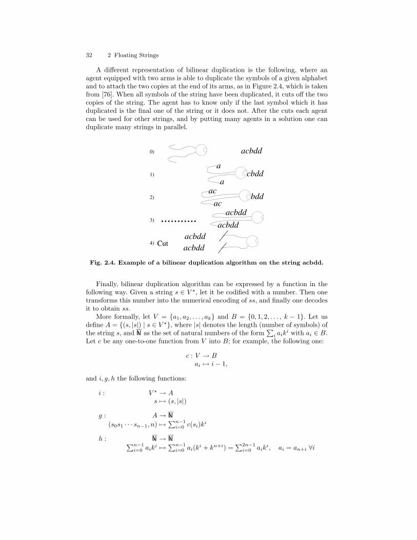
32 2 Floating Strings
A different representation of bilinear duplication is the following, where anagent equipped with two arms is able to duplicate the symbols of a given alphabetand to attach the two copies at the end of its arms, as in Figure 2.4, which is takenfrom [76]. When all symbols of the string have been duplicated, it cuts off the twocopies of the string. The agent has to know only if the last symbol which it hasduplicated is the final one of the string or it does not. After the cuts each agentcan be used for other strings, and by putting many agents in a solution one canduplicate many strings in parallel.
0)
1)
2)
3)
4)
...........
acbdd
cbdd
bdd
a
aac
acbddacbdd
ac
acbddacbddCut
Fig. 2.4. Example of a bilinear duplication algorithm on the string acbdd.
Finally, bilinear duplication algorithm can be expressed by a function in thefollowing way. Given a string s ∈ V ?, let it be codified with a number. Then onetransforms this number into the numerical encoding of ss, and finally one decodesit to obtain ss.
More formally, let V = {a1, a2, . . . , ak} and B = {0, 1, 2, . . . , k − 1}. Let usdefine A = {(s, |s|) | s ∈ V ?}, where |s| denotes the length (number of symbols) ofthe string s, and N as the set of natural numbers of the form
∑i aik
i with ai ∈ B.Let c be any one-to-one function from V into B; for example, the following one:
c : V → Bai 7→ i− 1,
and i, g, h the following functions:
i : V ? → As 7→ (s, |s|)
g : A→ N
(s0s1 · · · sn−1, n) 7→∑n−1
i=0 c(si)ki
h : N → N∑n−1i=0 aik
i 7→∑n−1
i=0 ai(ki + kn+i) =∑2n−1
i=0 aiki, ai = an+i ∀i
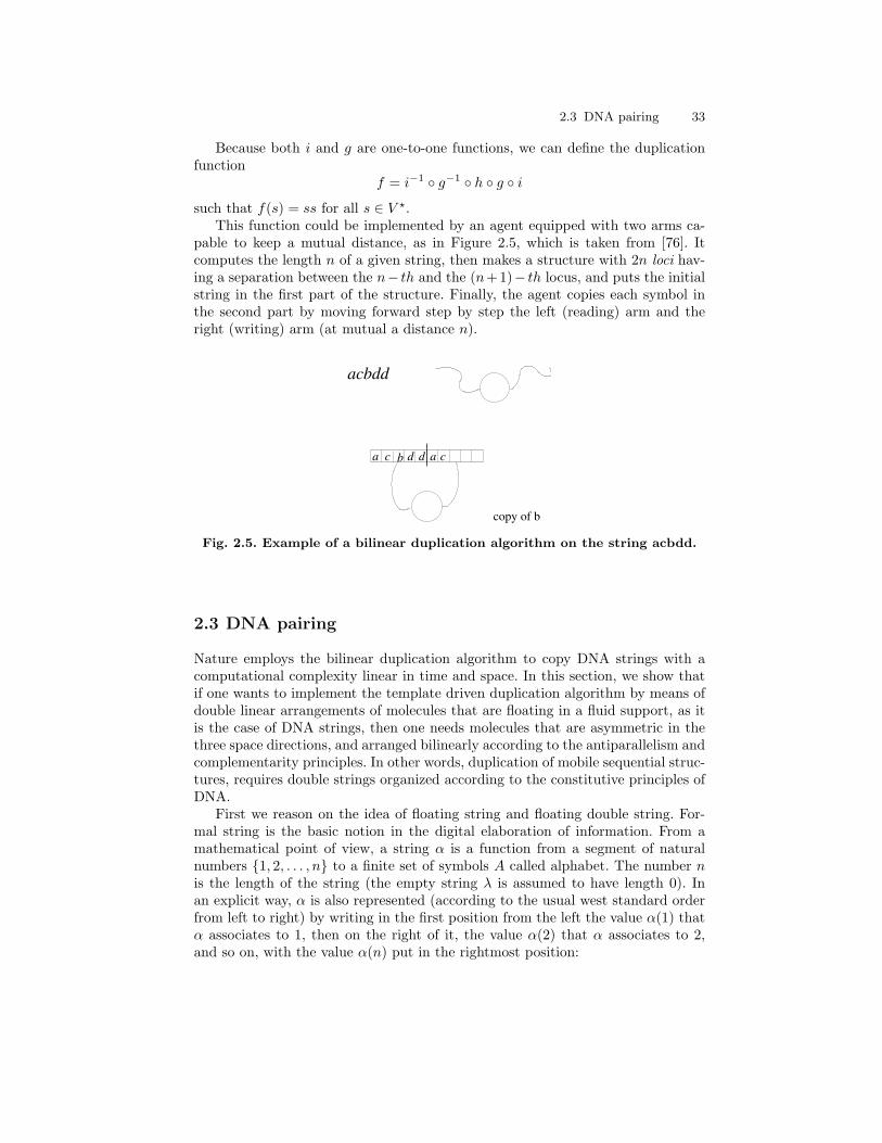
2.3 DNA pairing 33
Because both i and g are one-to-one functions, we can define the duplicationfunction
f = i−1 ◦ g−1 ◦ h ◦ g ◦ i
such that f(s) = ss for all s ∈ V ?.This function could be implemented by an agent equipped with two arms ca-
pable to keep a mutual distance, as in Figure 2.5, which is taken from [76]. Itcomputes the length n of a given string, then makes a structure with 2n loci hav-ing a separation between the n− th and the (n+1)− th locus, and puts the initialstring in the first part of the structure. Finally, the agent copies each symbol inthe second part by moving forward step by step the left (reading) arm and theright (writing) arm (at mutual a distance n).
a c b d d a c
acbdd
copy of b
Fig. 2.5. Example of a bilinear duplication algorithm on the string acbdd.
2.3 DNA pairing
Nature employs the bilinear duplication algorithm to copy DNA strings with acomputational complexity linear in time and space. In this section, we show thatif one wants to implement the template driven duplication algorithm by means ofdouble linear arrangements of molecules that are floating in a fluid support, as itis the case of DNA strings, then one needs molecules that are asymmetric in thethree space directions, and arranged bilinearly according to the antiparallelism andcomplementarity principles. In other words, duplication of mobile sequential struc-tures, requires double strings organized according to the constitutive principles ofDNA.
First we reason on the idea of floating string and floating double string. For-mal string is the basic notion in the digital elaboration of information. From amathematical point of view, a string α is a function from a segment of naturalnumbers {1, 2, . . . , n} to a finite set of symbols A called alphabet. The number nis the length of the string (the empty string λ is assumed to have length 0). Inan explicit way, α is also represented (according to the usual west standard orderfrom left to right) by writing in the first position from the left the value α(1) thatα associates to 1, then on the right of it, the value α(2) that α associates to 2,and so on, with the value α(n) put in the rightmost position:

34 2 Floating Strings
α(1)α(2)α(3) . . . α(n).
But, this notation hides a crucial point5. We can define α in this way because weassume that in writing and in reading the symbols on the paper they remain in theposition they were placed on, and also that the page has a standard orientationwith respect to the eyes of the writer and of the reader. If one is not allowed tomake these assumptions, this notation is useless. Even if all the symbols remaintogether, while leaving unchanged their relative position, one cannot uniquelyestablish what is the sequence associated to the linear arrangement given in thenotation above. In the case of mobile symbols indeed, the only way to recover thelinear order implicit in the notation above is to have an orientation, say left-right,in the symbols, in such a way that given a linear arrangement, we can distinguishthe first symbol of this structure, say the symbol having nothing on the left, fromthe last symbol, having nothing on the right.
Concatenation (usually indicated by juxtaposition) can be applied only be-tween strings oriented in the same way (from a biochemical viewpoint, ligase en-zyme performs the ‘fusion’ only of → or ← links, while working as in Figure 3.7,which is taken from [85]). Indeed, we can assume an axiom regarding the concate-nation direction:
• Concatenation Direction. Mobile strings require that each molecule has tobe asymmetric with respect to a ‘concatenation direction’ and concatenationhas to be performed between strings with the same verse along this direction.
The usual reverse operation on strings rev(a1 . . . an−1an) = anan−1 . . . a1 infact reverses the concatenation verse of a string.
In order to pair oriented strings, mobile symbols that are already oriented alonga direction, say x, need to possess another direction, say y, where two pairingsymbols connect. If we assume that no more than two floating strings can bepaired, then each symbol must have only one pairing link in the direction y andthis implies an asymmetry with respect to this direction.
• Pairing Direction. Bilinearly paired molecule strings require that eachmolecule has to be asymmetric with respect to a pairing direction.
In fact, assume to have two pairing links in the y direction (symbols shaped inthe following way la), in this case we could obtain multiple paired structures ofthe following type:
lαlα′
lαlα′
.
Instead, if one has the strings α = abaa and α′ = a′b′a′a′ in the double structureαα′ , then it must have the following shape:
↓ a ↓ b ↓ a ↓ a↑ a′ ↑ b′ ↑ a′ ↑ a′
5 J. Bennett. The difference between right and left. American Philosophical Quaterly,7:175-191, 1970.

2.3 DNA pairing 35
or in a more compact way:↓ α↑ α′
and the verse along the y direction is essential in order to have a binary pairing.The following alphabets comprise of the symbols from an alphabet V where
concatenation and pairing verses are explicitly indicated.
• ↑ V →def= {↑ w → | w ∈ V }
• ↓ V →def= {↓ w → | w ∈ V }
• ↑ V ←def= {↑ w ← | w ∈ V }
• ↓ V ←def= {↓ w ← | w ∈ V }.
Therefore, we can define the floating or mobile strings as the elements of thefollowing language [76]
W � = (↑ V →)? ∪ (↓ V →)? ∪ (↑ V ←)? ∪ (↓ V ←)?.
Actually, for notational convenience, in this thesis we will not use this termi-nology, but we continue to use the standard implicitly oriented letters to denotesymbols of alphabets. However, these speculations help to be aware of what thereis behind our usual formalizations, and highlight asymmetries of the molecule thatare not just due to chemical reasons but also to informational reasons.
Now we consider briefly the algorithm BDA in the context of the mobile strings,while further and more formal argumentations can be found in [76,148]. We knowfrom the physical implementation of chemical bonds that those acting betweentwo equal molecules are covalent bonds, that are very strong. In fact, for reasonsof symmetry, the common electrons responsible of the bonds are uniformly sharedby the two components. But, as we have seen in the previous section, the pairingduplication is based on the possibility of separating the two components of a doublestructure, in order to ‘recover’ from each of the strings the other one.
This means that the basic step of BDA duplication α • w βγ → α w • β
γ w resultsan oversimplification, and has to be replaced by α • w β
γ → α w • βγ h(w) where h is
a map such that h(x) 6= x for any symbol x, and it is an involution (h2 is equalto the identity) that associates mobile symbols to mobile symbols with opposite ydirection. In fact, when the algorithm starts on a string α and, after the separatingstep, it obtains the couple (α, h(α)), it continues to work on both strings, soobtaining a first couple (α, h(α)) from α, and a second couple (h(α), h2(α)) fromh(α) (and so on). It is clear that the algorithm performs a duplication only ifhk = I for some k > 0, and in this case k steps are necessary for obtaininga second copy of the initial string. Therefore, in order to satisfy the conditionh(x) 6= x the minimum value of k is 2, and the function results to be bijective.
The function h must to be extended to a morphism on the floating strings, westill call it h, in order to express the duplication process of the bilinear duplicationalgorithm, where the lower string is obtained by applying h to each symbol ofthe upper string and then by concatenating the results. More precisely, h(αβ) =h(α)h(β) for all α, β strings of W �.

36 2 Floating Strings
As a consequence of the existence of such a function h, the alphabet of mobilesymbols (on which it is an involution and it is different from the identity for everyargument) must obviously have an even number of elements. Two would be theminimal number for satisfying all the principles on which pairing duplication isbased on, but nature uses four elements. However, since a double linear structureis composed of two single complementary strings, if these strings vary over analphabet with just two symbols, then all the double linear structures with the samelength would be equivalent. In other words, if we use four symbols, then we get theadvantage to have an additional binary code written on the double stranded strings(if 0 expresses the pair bond A-T and 1 the pair bond C-G, then a double strandedDNA molecule identifies a binary string) [76]. It seems reasonable that nature doesnot underestimate this informational advantage. Namely, conformational aspectsseem linked to this second code.
Antiparallelism
We notice that floating symbols need to be asymmetric with respect to a third(with respect to concatenation and pairing) direction, in order that each strand ofthe double structure is the h-image of the other one.
In fact, if mobile symbols were two-dimensional objects or symmetric withrespect to the third space direction, say z, then after turning up-down the verse ofthe z axis, we would get the same shape. In this case only the two directions x andy would be relevant for catenation and pairing (one could avoid to consider the zdirection). This possibility though would allow us to get such kinds of pairings:
y
x
6
-
? ?? ?y
6
� xy
-6
x
y
yyy
yx
xxxx
�
6
----
where, the upper string is paired with two lower strings that cannot be concate-nated because they do not have the same catenation verse. Since any lower stringis the image of the corresponding upper string, under the morphism h from W �
to W �, a string can be paired only along a line ‘parallel’ to the ‘catenation line’and with only a string placed along this line.
Therefore, we can assume to orient the z axis of a molecule in such a waythat the pairing site of the molecule is placed in the region of points with the zcoordinate strictly positive.
• Third direction. Symbols of mobile strings must have a third direction, sayz, and must be asymmetric with to respect to this direction.
Moreover, for biochemical motivations (for example, enzymes read both strandsof molecules from the same side) it is reasonable to suppose that the pairingconnection is established between sites that are located at a ‘minimal distance’.
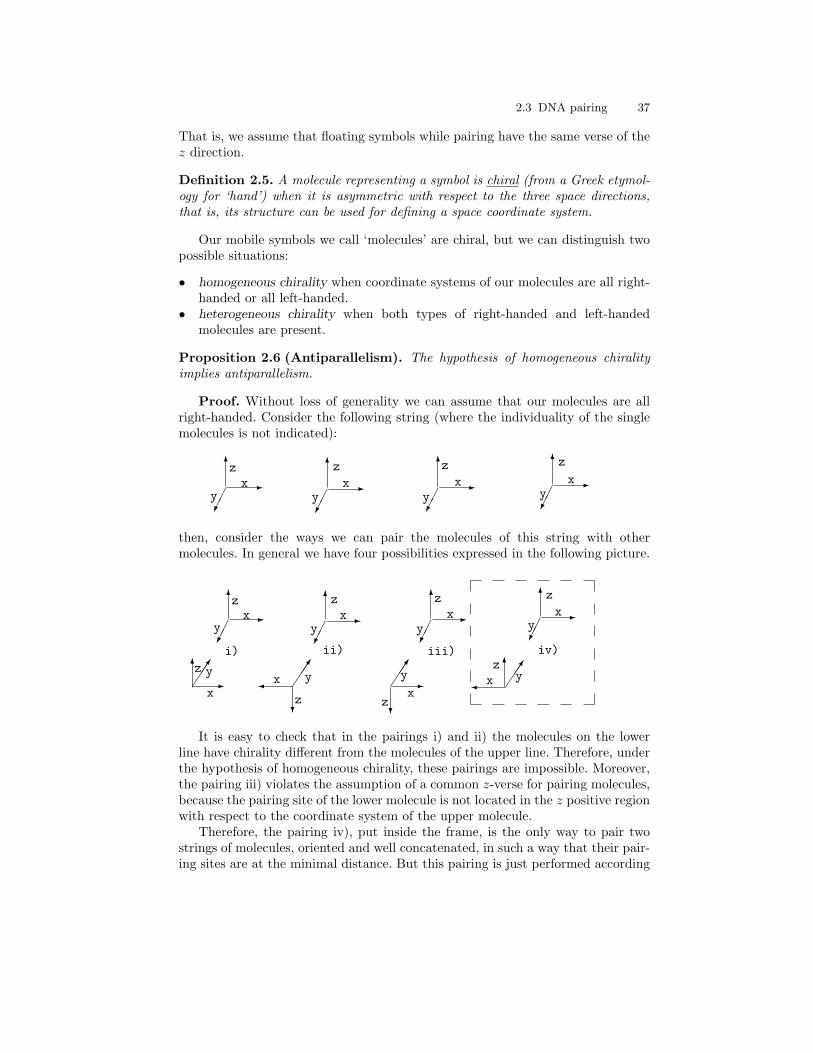
2.3 DNA pairing 37
That is, we assume that floating symbols while pairing have the same verse of thez direction.
Definition 2.5. A molecule representing a symbol is chiral (from a Greek etymol-ogy for ‘hand’) when it is asymmetric with respect to the three space directions,that is, its structure can be used for defining a space coordinate system.
Our mobile symbols we call ‘molecules’ are chiral, but we can distinguish twopossible situations:
• homogeneous chirality when coordinate systems of our molecules are all right-handed or all left-handed.
• heterogeneous chirality when both types of right-handed and left-handedmolecules are present.
Proposition 2.6 (Antiparallelism). The hypothesis of homogeneous chiralityimplies antiparallelism.
Proof. Without loss of generality we can assume that our molecules are allright-handed. Consider the following string (where the individuality of the singlemolecules is not indicated):
-
6
���
���
6
-�
��
6
-�
��
6
-x x x xy y y y
z z z z
then, consider the ways we can pair the molecules of this string with othermolecules. In general we have four possibilities expressed in the following picture.
iv)iii)ii)i)
z z
z
zzzz
z-
?
6
�
�x y-
6
�
x
y
?
�
�x y
yyyy
y
x
xxxx
�
-
6
���
-
6
���
-
6
���
���
6
-
It is easy to check that in the pairings i) and ii) the molecules on the lowerline have chirality different from the molecules of the upper line. Therefore, underthe hypothesis of homogeneous chirality, these pairings are impossible. Moreover,the pairing iii) violates the assumption of a common z-verse for pairing molecules,because the pairing site of the lower molecule is not located in the z positive regionwith respect to the coordinate system of the upper molecule.
Therefore, the pairing iv), put inside the frame, is the only way to pair twostrings of molecules, oriented and well concatenated, in such a way that their pair-ing sites are at the minimal distance. But this pairing is just performed according

38 2 Floating Strings
to the well-known antiparallel concatenation verse. ut
In a very intuitive way, the situation described above is analogous to whathappens in a folk dance where a line of dancers is paired to another line of dancers.The concatenating verse of x is from the left to the right of the body, where handsjoin, the pairing verse of y is from the back to the face of the body, and the zdirection is the vertical axis with the usual verse. The pairing sites are on eyes, sothat each dancer pairs with the opposite dancer by meeting his/her sight. Each linehas a catenation start where there is a dancer with nobody on the left side. Thechirality of human body implies that there is no arrangement different from theantiparallel way for matching the two lines of dancers, in the sound (face-to-face)correspondence [76].
The case of homogeneous chirality corresponds to the real case of DNA, whilein the case of heterogeneous chirality the antiparallelism is replaced by a morecomplex principle:
Proposition 2.7. Under the hypothesis of heterogeneous chirality, a molecule canpair either only with a molecule with different chirality in a parallel way, or onlywith a molecule of the same chirality in an antiparallel way.
In fact, if both right-handed and left-handed molecules can belong to the stringin the (for example) upper line of a double structure, then, from all the aboveassumptions, the possible pairings are reduced to ones in the following picture.
? ?
-6
���
���
-���
-���
6-
�
x xx x
x
y
y yy y
yx� �
?
yx
�6
-yx� �6
?
-z
z
zz
z
z
z z
i)iii)ii)
iv)
Therefore, a molecule can only pair either with a molecule with different chiral-ity in a parallel way, cases i) and ii), or with a molecule of the same chirality in anantiparallel way, cases iii) and iv). If both possibilities are allowed, then we wouldhave molecules with different catenation verses in the lower line of a double stringstructure, that is forbidden by the correctly working of the bilinear duplicationalgorithm.
In this dissertation, as usual, the length of a string α is denoted by |α|, and itspairing (complementary and with opposite concatenation orientation) string by α.
2.4 DNA-like computations
The rules of the bilinear duplication algorithm that are described in Section 11have a clear biotechnological implementation. In fact, the doubling step can beperformed by a polymerase enzyme, and the separating step by a denaturation

2.4 DNA-like computations 39
operation, due to an increase of the temperature. While the first step is just theformal passage from a single string to a string placed into a double structure. Thebiological interpretation of the symbol • is related to the orientation of the string:the computation starts only when it is at the beginning of a string with respectto the concatenation verse, enzymes can recognize this point from the chemicalstructure of the molecule.
In this section we propose a universal (DNA-like) system which computes ondouble structures of mobile strings by means of rewriting rules that have a biotech-nological implementation. Essentially three types of operations are enough in orderto obtain universal computations, as one can see from [160,161,162]; they are du-plication, triplication, and division by six. Our system processes the informationencoded on floating strings by simulating these three operations. It is able to ex-ecute any program of a register machine, since it has also a mechanism to switchfrom one instruction to another one and to perform jump instructions.
This system is an extension of the floating bilinear duplication algorithm. Infact, (from a theoretical point of view) the computation can be implemented onDNA strings; but the crucial difference is the encoding used to represent numericalinformation by a floating string. The output of the bilinear duplication is given bytwo copies of the initial string, and from the same viewpoint, the product of thetriplication would be given by three copies of the initial string and the divisionby six would reduce six copies of the string to one copy. That is, the numericalinformation which is processed by the operations consists of the number of copies ofthe initial string. Here instead, we consider the information as completely carriedby (one copy of) the current string, regardless to the number of copies of sucha string. It is transformed by means of operations in each step of computation,as usually on the tape of a Turing machine. The initial string encodes the givennumerical input, and when one of the operations modifies it, the string encodingthe number obtained after the application of that operation is produced.
Let V be the alphabet with four symbols {1, 2, 3,#}, and n a numerical in-put. The factorization in primes of n can be seen as 2km 3h, with m ∈ N andnon-divisible by 2 or 3. Since every m can be written in unary code, then everynumerical input n can be considered as a particular string over V , with a numberk of 2s as prefix and a number h of 3s as suffix that are uniquely implied by thevalue of n. In particular, we associate n to the string ↓ 2k#m#3h →, and we referto it simply with 2k#m#3h belonging to V ?.
A DNA-like system
We present a formal system based on the double string structure of mobile strings,that is able to duplicate, triplicate, and divide by six a number n (representedby a string encoding as above), and to switch from performing one instruction toanother one of a register machine program. By [159,160,161,162] we know that thissuffices in order to perform universal computations, as all the basic instructionsof a register machine can be reduced to “times 2” or “times 3” or “division by 6”instructions.
With our encoding, in order to duplicate a number it is enough to juxtaposethe symbol 2 at the beginning (with respect to the concatenation verse) of the

40 2 Floating Strings
string encoding the number, and in order to triplicate one has to concatenate thesymbol 3 at the end. The division by six is performed by eliminating the first andthe last symbol of the string if both of them are different from #, otherwise thenumber is not divisible by six.
The system works with deterministic rewriting rules over double string struc-tures, where a special meta-symbol of kind • marks the point of progress of thecomputation. In particular, we consider different pointers corresponding to the pinstructions of the program we want to simulate, they belong to the set Q of point-ers and have an index representing an instruction label, Q = {•1, •2, . . . , •p, . . .}.In the case of instructions which are decrements, that correspond to divisions [159],during the computation we use further (primed) indexes, among {1′, . . . , p′}; how-ever the number of our pointers, that is the cardinality of Q, is bounded by 2p,where p is the number of the instructions of the given program.
In the following, we have three groups of rewriting rules, where λ denotes theempty string (in V ?), α, β, γ, ξ ∈ V ? with β, ξ 6= λ, whereas a, b ∈ V , j ∈ {1, . . . , p}and j′ ∈ {1′, . . . , p′}. We refer to ξ′ to denote the string obtained from ξ afterhaving erased its first symbol.
1. Starting
2k#m#3h −→ •1 2k#m#3h
λ
This step marks the start of the computation, by transforming the input fromsingle string into double string structure. After such a step the first instructionis going to be executed, as required by the presence of the pointer with index 1.
2. This multiple step performs the operation indicated by the jth instruction ofthe program (whenever it can be performed), for j ∈ {1, . . . , p}, that can be aduplication, a triplication, a jump, or a division by six.
a) Doubling (for j belonging to the labels such that the corresponding instruc-tions are duplications)i. •j a α
λ−→ a •j α
2aii.
γ •j a α2γ
−→ γ a •j α2 γ a
b) Tripling (for j belonging to the labels such that the corresponding instruc-tions are triplications)i.
α •j a βα
−→ α a •j βα a
ii.α •j aα
−→ α a •jα a 3
c) Jumping from j to l (if the label j corresponds to an instruction which isa jump to the l-th instruction)

2.4 DNA-like computations 41
•j αλ−→ •l α
λ
d) Dividing by six if possible, otherwise jump from j to l instruction (j be-longing to the labels such that the corresponding instructions are divisionsby six, which can be performed if, and only if, both the first and the lastsymbol of the current string are different from #)i.
•j 2 αλ
−→ 2 •j αλ
ii.•j # α
λ−→ •l # α
λ
iii.ξ •j a βξ′
−→ ξ a •j βξ′ a
iv.ξ •j 3ξ′
−→ ξ 3 •jξ′
v.ξ •j #ξ′
−→ ξ # •j′ξ′ #
vi.ξ •j′ξ′
−→ ξ •j′•l 2 ξ′
3. Switching and Separating
a)α •jβ−→ α •j
•j+1β
b)α •i•j γ
−→ •j γλ
c)•p+1 γ
λ−→ γ
Whenever a string which is preceded by the pointer •p+1 is transformed in asingle string (that is the step 3 part (c) is executed), then the program halts andthe single string encodes the numerical result of the computation.
Given a register machine program, all its basic instructions of increasing by 1,decreasing by 1, and testing if a register contains 0 or not, may be simulated bya program with p labeled instructions that double, triplicate, or divide by six thenumerical information, or represent a jump. In the above system the first step isperformed only at the beginning of the program. Then, whenever the current labelj points to a doubling or a triplicating instruction, the rewriting rules of the step 2,

42 2 Floating Strings
part (a) and part (b) respectively, are applied in a deterministic way. In both thesecases the operation is completed when no other rule related to that operation canbe applied, and a double structure of kind α•
β is finally obtained. If label j refers toa jump, the rule of the step 2 part (c) is applied, so that the operation labeled byl can be performed. If j corresponds to a division by six, then the rewriting rulesof the step 2 part (d) are applied. If the current string begins with the symbol 2and ends with the symbol 3 (that means that it represents a number divisible bysix, and the division can be performed), then the computational process leads toobtain a double structure of kind α•
β . Otherwise, a jump is performed whenever thefirst symbol is equal to #, and a double structure of kind α•
•β is obtained wheneverthe last symbol is equal to #.
The switching and separating rules of step 3 lead deterministically the compu-tation to perform the next operation, or to give out an output. In particular, the(a) rule switches to the next instruction (the (j + 1)th one), after that the oper-ation j has been performed regularly, while the (b) rule allows the correspondinginstruction to start even after an operation of division by 6 which was not per-formed. The (c) rule is applied at the end of the program, and it gives out thecurrent string as output.
Note that we have an alphabet with exactly four symbols and the typical DNAstring double structure. Moreover, the biochemical implementation of the mainstep (the second one) recalls the work of a special polymerase, since symbols arecopied from a template by elongating a primer with concatenation, and the verylast step recalls the annealing process.
In the case of duplication, a translation of the first symbol a into the string 2ahas to be done (i.e., a symbol 2 and a symbol a are juxtaposed as lower string ofthe double structure) before performing the copying of the remaining string, andin the case of triplication, a translation of the last symbol a into the string a3 hasto be done after a usual copying of the string. While in the case of division, thecopying is performed after the elimination of both the first and the last symbol ofthe string.
There are some enzymes called exonuclease (see Section 5.2) with the ability tocut away the extremal symbols of a string. Unfortunately, from an experimentalpoint of view, it is really difficult to control these enzymes in such a way thatonly one letter is removed. At a theoretical level though, in all these cases, thenatural orientation of the DNA strings is a mechanism to recognize which is thefirst symbol and which is the last one of a string, and enzymes as polymerase orexonuclease are able to recognize these points.
The exchange of pointers and the appearing of a pointer in the lower stringcan be seen as indications corresponding respectively to what enzyme is going toread and copy and from where. In DNA computations, the enzymes are chosenby humans, and the point of progress of the computations is given by the naturalorientation of DNA strings.

2.5 Membrane systems 43
2.5 Membrane systems
To achieve the realization of microscopic computers, it is necessary to learn asmuch as possible from the biology of the living cell, that is currently the onlyknown DNA-based molecular computer in existence. Cells were observed for thefirst time about three hundreds years ago, right after the construction of the firstmicroscopes. In the second half of the nineteenth century it was already clear thatthey represent the smallest and irreducible unities of life of which every organ-ism is comprised. Eukaryotic cells keep together the genes, the RNAs with theproteins which they encode, as well as the products of their activities. Cellularcompartmentalization is the key of the organization of biomolecular systems, suchas networks of proteins underlying the main cellular functions, and it is essentialfor the evolution of all living organisms.
Models based on abstract process languages use the ‘compartment-as-process’abstraction. Though the most inherent works, such as Petri Nets [92] or processalgebra [172], do not handle compartments explicitly, with some exceptions, whereabstraction of movement of and between compartments is however either limitedor completely absent [165,192].
In this section membrane systems are proposed as a model to represent var-ious aspects of molecular localization and compartmentalization, including themovement of molecules between compartments, the dynamic rearrangement ofmolecular reactions, and the interaction between molecules in a compartmental-ized setting (for a brief introduction to the model see Section 1.1.1, and for apicture of a membrane structure see Figure 2.6).
There exist similar models motivated by ambient calculus, a process algebrafor the specification of process location and movement through computational do-mains, that have a flavor of biology [192, 34]. Indeed, in this paradigm of mobilecomputation [35], each ambient harbors a collection of processes, that reside andrun directly within it, and the processes inside an ambient control it, by instruct-ing it to move. The biochemistry of the cell works differently though. The natureof each process (which can be a transformation, a duplication or an expelling ofmolecules across cell membranes) is relevant as it changes the environmental condi-tions for the other processes and not only in the same compartment. For example,until DNA has been ‘translated’ into mRNA the corresponding protein cannot besynthesized, because the information is not present yet. Moreover, the organizationof compartments do not depend directly (often at all) on the processes inside them(e.g., the nucleus of a cell is there in any case). Cell membranes can duplicates,can be dissolved and created, and usually it depends on environmental conditions.Finally, an important point of biological relevance is the interest to the molecularreactions themselves rather than only to their distribution and coordination incompartments. Therefore, in this context, considering computational processes aselementary objects would be quite reductive.
Membrane systems, also named P systems, were inspired by cell biology in theirformulation6. Since they were introduced [178], they have been widely investigatedas models and tools of interest for computer science, and although still “dynamic
6 “Membrane computing is a branch of natural computing which abstracts from thestructure and the functioning of living cells”, Gh. Paun, first sentence of the book [180].

44 2 Floating Strings
P systems are not well developed, rendering them limited in their applicabilityto biological systems” (A. Regev, E. M. Panina, W. Silverman, L. Cardelli, andE. Shapiro, [192]), many works have successfully advanced the state of the art inthis direction [43], and the intent to employ membrane systems as a frameworkto study real biological systems is vividly pursued [24,149,12,18,66,25] (“Makinguse of both the theoretical developments and of the existing implementations, MCstarted to be used as a framework for modelling biological processes, especially atthe level of the cell.” Gh. Paun, [181]).
A membrane structure is a string of matching enumerated brackets; such as:
[1 [2 ]2 [3 ]3 [4 [5 ]5 [6 [7 ]7 ]6 ]4 ]1
that can be represented as well by the diagram in Figure 2.6.
1
2
3 46
7
5
membranes regions
Fig. 2.6. Example of a membrane structure, where membranes and regionsare pointed out.
An evolution rule is a string rewriting rule of the form
u→ v
where u is a string over an alphabet O, and v is a string over O × TAR,where TAR = {here, out} ∪ {inj |1 ≤ j ≤ m}. These rules represent the chem-ical reactions residing in the compartments of a cell. For example, the ruleabc → (b, here)(d, out)(c, ink) means that three elements a, b and c react, pro-ducing a copy of b, d, and c. Moreover, b remains in the same region, d is sentoutside of the compartment, into the surrounding region, and c enters the directlyinner membrane labeled with k [181].
A standard definition of membrane system is the following, from [180].
Definition 2.8. A membrane system of degree m, where m ≥ 1, is a structure
Π = (O,µ,w1, . . . , wm, R1, . . . , Rm, io)

2.5 Membrane systems 45
where O is an alphabet, and its elements are called objects, µ is a membranestructure, with the membranes (and hence the regions) labeled by 1, 2, . . . ,m. For1 ≤ i ≤ m, wi and Ri are respectively the multiset of objects and the finite setof evolution rules over O associated to the region i of µ. Finally, io belongs to{1, 2, . . . ,m} and denotes the label of an elementary membrane, called output mem-brane.
Membrane systems are a discrete device (as only discrete quantities are in-volved) which takes explicitly in account the notion of compartments. The wayhow the evolution rules work recalls the computational strategies of formal gram-mars, that traditionally were applied to the analysis of biological structures [142].
Most recently, membrane systems were differently defined in [34], as a notiongrounded in process calculi that assumes concepts of metric and regularity offunctions. “A membrane is a curve in R2 that is closed, non-self-intersecting, andsmooth. A membrane system is a collection of membranes such that no two mem-branes intersect”, L. Cardelli, [34]. In this context, the Jordan’s Curve Theoremis called to assert that any membrane divides the plane into a bounded connectedinside region and an unbounded connected outside region.
If one thinks of chemical reactions that involve the same molecules and happenin parallel inside cytoplasm and nucleus of a cell, topological features of a modelseem to be important to simulate these processes. The concept of distance thoughis not necessary, at least at a certain level of abstraction. Let us explain by anexample: we suppose to have two molecules that interact (namely by transformingeach other) just by contact, instead of sending signals to each other. In this case,having a distance would be important; in fact, we could evaluate their relativedistance in any computational step of the system, and assume that they interactwhen this distance is zero. Such an approach allows even to estimate in how manysteps the two molecules meet each other in the system. On the other hand, in thisway we enter very much in details of processes, by loosing the ability to observethe global properties of the system. It might be better to say that those specificmolecules interact eventually, given that they stay in a same compartment (i.e.,‘close enough’), no matter when and how exactly. These speculations recall theconcepts of microscopic indetermination explained in Section 1.1 and the basicstrategy of forbidding-enforcing systems (see Sections 1.1.1 and 7.1).
Usually biomolecular phenomena are continuous in space and time. Though,in most cases, the information necessary to describe them is inherently discrete(think, for instance, of DNA replication). There are also cases in which a discretecharacterization of this information generates errors, but such errors can be ar-bitrarily reduced or, equivalently, the precision is proportional to the granularitywith which the continuous phenomenon is reproduced by the discrete model.
2.5.1 Some variants
The original model of membrane system was enriched with several other features,usually inspired by biology. We present here very few examples from the numerousvariants that may be found in literature.
A P system is called cooperative if it contains evolution rules with radius greaterthan one, where the radius of a rule u→ v is the length of u. A particular class of

46 2 Floating Strings
cooperative systems is that of catalytic systems, where the rules with radius greaterthan one are activated (i.e., can be applied) by the presence of special ‘catalystobjects’, which are not transformed. This kind of rules formalizes what happens inthe cell when some enzymes catalyze a molecular process that is enzyme enhanced.In the cell there are also chemicals that, while supporting or forbidding certainreactions, can separately evolve, in parallel with the chemicals involved in thereactions. These features were formalized in the context of membrane systems, bymeans of promoters and inhibitors, that are respectively permitting and forbiddingobjects associated to regions [27] (activators are a recent variant of catalysts andpromoters). Other powerful extensions of the membrane formalism are representedby the introduction of a priority relation among the rules from each region, in theform of a partial order relation, and by a polarization (associated to membranes)that controls the activation of some rules with respect to other ones.
The symport/antiport rules introduced in [176] are related to the exchange ofobjects between membranes: each membrane can communicate with other mem-branes by sending out objects that the other membrane can bring inside. A sym-port rule has the form (x, in) or (x, out), and an antiport rule has the form(x, in; y, out). These rules have a weight, which is given by |x| in the fist case,and by max{|x|, |y|} in the second case. Unlike most of the other variants of Psystems, this family has the feature that no objects of a system change during thecomputation; they only change their locations related to membrane label numbersin the system. For different types of P systems with symport/antiport rules it wasfound that there is not difference between the computing power of deterministicand nondeterministic systems. The symport/antiport systems were then extendedby evolution-communication P systems, where the objects are also transformed bymeans of evolution rules.
The symport/antiport rules were generalized by the boundary rules introducedin [19], that are not ‘located’ into regions but properly on the border of the mem-brane. In fact, the boundary rules are not ‘blind’: they are not internal to regionsbut they are able to ‘see’ even externally, that is, they are sensible to what hap-pens around the corresponding membrane. In a sense, membranes with boundaryrules have ‘windows’ to look at the environment. An analogous idea was devel-oped by [78] in another context, in terms of P systems with rules ‘assigned tomembranes’. In such a work, the strings involved in the splicing operation areeither taken from inside or from outside the membrane, and the strings resultingfrom the splicing operation also are able to go inside or outside the membrane.Together with splicing operations, also operations of cutting and recombinationwere used as rules assigned to membranes [78].
Finally, we recall the ‘conformon P systems’ as a simple variant of P systems;they replace the objects with ordered pairs of name (object) and (numerical) value,that is called conformon. They are universal systems introduced in [82] and recentlyimplemented in [83]. In fact, in most cases, membrane systems exhibit Turinguniversality and fast solutions to hard problems. The definition of complexityclasses of P systems is huge matter of investigation, whereas the descriptionalcomplexity measurements are usually given by the number of membranes, the size

2.5 Membrane systems 47
of rules, the number of objects. P systems with active membranes7 and only twopolarizations are universal and even able to solve SAT in linear time. Finally,a universality result has been obtained for systems with only two membranes,using only multiset evolution rules and sending objects out of a membrane whilechanging its polarization [3].
PB systems were proposed as a variant of P systems with boundary rulesin [19]. The authors proved the computational universality for PB systems withthree membranes which regard at most one symbol outside and one symbol in-side a membrane. They also investigated the relationships with the basic model ofP systems by proving an equivalence between P systems without priority, thick-ness or dissolution operator8, and PB systems that use communication rules ofrestricted form. The boundary notation α [i β → α′ [i β′ means that if thei-membrane contains the multiset β and the multiset α is present outside, thenthe multisets α′ and β′ are produced outside and inside the i membrane, respec-tively. The boundary notation can be extended naturally in several directions tocope with typical biological phenomena. Namely, the idea of membrane transportis well simulated by explicitly introducing membranes in the rules, as “boundaryentities” which control inside and outside of the delimited region [19]. In PB sys-tems, communication is allowed by general rules of the form α [i β → α′ [i β′,because if the membrane i contains the multiset β and the multiset α is presentoutside the membrane i, then a “communication” can be established by producingthe multisets α′, β′ outside and inside the membrane i, respectively. Moreover,with respect to [176], transformation rules [i β → [i β′ are allowed in PB systems.
An advantage of boundary notation is a more compact definition of P systems.In fact, according to [180] and to the definition given in the previous section, aP system is a structure Π = (A,µ,w1, . . . , wm, R1, . . . , Rm, io) that is, alphabet,membrane structure, words inside regions, rules relative to regions, and outputmembrane. If we use the boundary notation, we can define a P system in a moreconcise way9 as
Π = (O,µ,R, io)
with O alphabet, µ the whole initial membrane system configuration (includingboth membranes and multisets of objects), R a finite set of boundary rules that(apart the objects which they transform) contain explicitly in their expression alsoon which membrane of the system they work, and io the output membrane. If weare studying the life of the system instead of what language it computes (that is,we are interested only to the evolution of the system from the initial configurationµ), then we can even consider just the structure Π = (O,µ,R).
In [75] we extended the boundary notation to describe new kinds of rule sug-gested by typical phenomena occurring in cells. A first task has been the for-malization of the very important concept of cellular receptors, which are pro-7 They are membranes able to duplicate, or, more in general, membranes with the ability
to dynamically change the membrane structure µ of the system [178].8 ‘Thickness’ and consequent permeability to entrance of objects can be associated to
membranes by means of operators [180].9 As suggested in: G. Franco, V. Manca, String Models and String Dynamics, TR of the
EMCC (European Molecular Computing Consortium) Meeting, p 17, Turku (Finland),May 15-17, 2003.

48 2 Floating Strings
tein three-dimensional forms that recognize and fit with their specific counter-receptors. For example, the immunological process of the selective recruitment ofleukocytes starts when the receptors located on leukocyte cells surface bind withsome ‘counter-receptors’ located on the surface of endothelial cells, and these bondsslow down the initial speed of leukocytes in the blood.
From a membrane computing point of view, the notion of location due to thepresence of compartments needed to be extended. In fact, objects in the membranesystem usually may reside either inside or outside a given compartment. Receptorsinstead reside across a membrane boundary, and in a sense belong to two com-partments, because they can ‘see’ both internal and external regions. In [75] thisparticular phenomenon was studied and a notation in double bracketing fashion[i [i ]i ]i allowed us to deal with ‘receptors’ (that are ‘sensors’ located on the cellsurface in order to capture external signals) as with objects ∗ that can stay onlyinside the interstice of a double membrane [i ∗ [i ]i ∗ ]i.
By extending the boundary rules we have been able to model cellular dynamicswith membranes, because we could modify the topology of a membrane structure.Namely, we model the moving of a membrane with its whole content into anothermembrane, as well as the generation of a ‘tissue’ by adhesion between membraneswith the same label. Also, we modeled typical processes occurring in the cells,such as external signalling for receptor activation, adhesion between membranesby receptor affinity, production of internal signals, internal signalling for receptoractivation, phagocytosis (with diapedesis and opsonization as particular cases),expulsion (as inverse of the phagocytosis), fusion, lysis, and apoptosis as a combi-nation of affinity adhesion and lysis.
An important aspect in modelling biological reactions by rewriting rules is therule application strategy. Nondeterministic maximally parallel way or other math-ematically elegant strategies are not realistic. Percentages of reactivity assignedto rules would seem a better idea, but still several strategies can be performed. Infact, with regards to the BZ oscillator in [224], the same percentage of applicationscan give very different behaviours with rules applied in a different order. It seemedto us that both the order is essential and the reactivity parameters must dependon the concentration of certain objects in some membranes.
In this context, a novel perspective has been recently introduced by V. Manca’sgroup [21, 149]. This is the idea of controlling the evolution of a (membrane) sys-tem by means of rules whose strength and application depend on the objects con-centration. Rules are specified along with dynamical reactivities, called reactionmaps. Every reactivity denotes the ability of the corresponding rule to competeagainst other rules in capturing part of the population on which the reaction is per-formed [23]. By going ahead in this perspective, every reactivity has been identifiedto a map that depends on the state of the system, and a strategy has been addedfor partitioning the objects in the system at every transition, by depending on therelative magnitude of every reactivity [22]. This new strategy of rule applicationwas inspired by real ‘metabolic reactions’, and it seems to lead membrane comput-ing towards interesting simulations of biological processes, such as representationsof signal transduction networks and complex oscillations [24,66,25].

2.5 Membrane systems 49
2.5.2 Applications
P systems as well as any biomolecular computing device, are at an initial devel-opment stage. On one hand, their simplicity does not limit their computationalpower and, in fact, numerous results of universality were proven. On the otherhand, much research has still to be done to get them closer to the world of real(especially, but not only) biomolecular applications.
However, many recent, very promising works in this direction can be found inthe book [43] and in the Proceedings of the first workshop on Theory and Ap-plications of P Systems (TAPS), held in Timisoara in September 2005. Multisetprocessing in the compartmentalized framework provided by cell-like or tissue-likemembrane structures turned out to be a widely applicable modelling techniquein several domains, such as biology (for mechanosensitive channels, respiration inbacteria, photosynthesis), medicine (for immunological processes, signalling path-ways), economics10, linguistics, computer science (computer graphics, cryptog-raphy, approximate solutions to optimization problems). Computationally hardproblems have been investigated through P systems (for example, in [93]), andproblems coming from classical bioinformatics have provoked interest as well. Forexample, in [67] seven algorithms to find the maximum of a set of numbers weresystematically investigated in terms of P systems, on the way to find better solvingmethods for the multiple sequence alignment problem.
In [21] we have focused our effort in addressing some theoretical and practicalissues especially oriented to biomolecular computing—this applicative directionbeing followed also by other groups (see, for example, [7, 18]). There are someaspects, that are crucial in many studies of biomolecular processes, that the tra-ditional formulations of P systems do not take into explicit account:
1. dynamics of biosystems. The dynamical behaviour of biomolecular processeshas a major relevance in the description of the processes themselves. Thismeans that two or more processes that terminate with identical configurationsmay move through completely different transitions. Think to the physiologyof distinct human beings: we know that the biomolecular processes happeninginside them inevitably move towards a well-determined terminal state. Rather,we would be interested in the trajectory followed by these processes, i.e., theset of intermediate states forming each trajectory.
2. process evolution. The halting of a P system tells that a computation hasterminated successfully. For what we have written at the previous point, theterminal state is not a primary object of investigation in many biomolecularexperiments. Rather, one should shift the focus on the computation during its“life”, in the aim to investigate the strategies that a living organism puts intoaction to survive in certain environmental conditions.
3. environmental energy and resources. The resources available in the environ-ment play a major role in the control of a biomolecular process. The existencein the environment of elements, which can act as catalysts or provide the en-ergy needed for the biochemical elements to react, can radically change the
10 Gh. Paun, R. Paun. Membrane Computing as a Framework for Modeling EconomicProcesses. Submitted.
50 2 Floating Strings
nature of a process. In particular, an environment which periodically feedsthe system with resources can transfer properties of periodicity to the systemitself [20].
4. locality of the system control. Biomolecular processes are the result of manyindividual reactions, each one of those being formed by subprocesses whose ex-tension is limited in space and in time. These subprocesses get the informationon what is happening in the whole organism by their respective neighborhood.Though, they often exhibit a surprising overall coordination, and in this sensebiomolecular processes are by all means asynchronous.
Clearly, these aspects are closely related one to the other: shifting the focus onthe system dynamics means that less attention is payed to the final configurationof the system; meanwhile, the continuous control of the resources needed for theprocess to evolve is fundamental to drive the system dynamics along a specifictrajectory. The environment itself has the role of a “supervisor” in the processcontrol, since it becomes responsible of a sort of external input, whose effects inthe system propagate via local reactions.
About the first point, usually P systems are intended to “consume” the avail-able resources in a nondeterministic and maximally parallel way during the rewrit-ing of symbols. In particular, the latter condition prevents the system to accountfor specific evolutions within a transition. In principle, one may try to increase thegranularity of a P system in order to obtain fine-grained sequences of transitions,then consider the trajectories described by these sequences, and this descriptionwould be as accurate as fine the granularity of the P system is. In practice, it islikely that the desired granularity is obtained by adding auxiliary symbols or prior-ity constraints in the system, to form (sometimes complex) priority relationshipsfor the rewriting rules. As a matter of fact, P systems do not provide tools forcontrolling the resolution of the observation of intermediate states; they are bettersuited to model a process as a sequence of “snapshots”, each one being taken whenno more rewriting rules can be applied.
About the second point, there are cases in which a nonterminating process givesmore insight than a terminating one. Nonterminating processes, in particular, areof key importance in the study of periodicity and quasi-periodicity, two aspectswhose detection is important for understanding many biological processes. Fromthis viewpoint, traditional types of P systems do not provide versatile tools tohandle periodicity.
The question of resource availability is unavoidable in the study of biomolec-ular phenomena. P systems, in their native definition, did not take any energeticconstraint into account. It was feasible for them to use indefinitely large amountsof resources to perform a computation, whereas this cannot happen in nature.Further types of P systems have been proposed in which energy is consideredas a constraining factor (see, for example, [187]), although in those systems theenvironment is intended as a place to exchange resources and has not a centralrole.
Finally, P systems are traditionally organized in a way that their evolution issynchronous, i.e., a global clock triggers the production of new symbols inside allmembranes. This aspect, that limits their versatility in modelling asynchronousphenomena, has been recently addressed in [36].

2.5 Membrane systems 51
In [21] we considered a different perspective (for many aspects still in progress)according to which P systems were cast in a dynamical framework. In this perspec-tive, we characterized transitions and space states of a discrete dynamical systemby means of state transition dynamics [151]. Concepts of periodicity and quasi-periodicity of state transition dynamics were applied to P systems with boundaryrules and dynamical environment (PBE systems); in particular, the Brusselator(a famous chemical reaction) was successfully simulated.
Overall, a new way to observe the evolution rules of a system reproducing areaction was proposed. Indeed, since the application of every rule changes the rel-ative amounts of reacting substances, it was imposed that such a relative amountinfluences the reactivity of the rules in a way that their application depends onthe current substances concentration, as it normally happens in biochemical phe-nomena. A simulator applying evolution rules with this strategy (named Psim)was developed and used to simulate some processes [21]. In fact, an applicationof this strategy to problems so far described in terms of differential equations wasproposed, beside a simulation with Psim of mechanisms typical of the leukocyteselective recruitment process activated against an inflammation.
Due to its complex nature and capability to rapidly adapt to the attack ofinfectious agents, the immune system may be considered a typical example ofcomplex adaptive system [216]. A formal description has been developed in [75]about the phenomenon of leukocyte recruitment that plays a critical role in theimmune response. In a next step, the leukocyte selective recruitment has beenmodelled (under some constraints that simplify the dynamics of the system) as adynamical system of interactions between leukocytes and endothelial cells in [21],where an extended version of membrane systems turned out to be a very usefultool in the formal analysis of the recruitment process.
Leukocyte selective recruitment
The first response to an inflammatory process in a given organism activates atissue-specific recruitment of leukocytes that relies on the complex functional in-terplay between the surface molecules that are designed for specialized functions.These molecules are differently expressed on leukocytes circulating in the bloodand on endothelial cells covering the blood vessel (see Figure 2.7, which is takenfrom [75]).
Three major steps have been identified in the process of leukocyte recruitment:i) tethering-rolling of free-flowing white blood cells, ii) activation of them, and iii)arrest of their movement by means of their adherence to endothelial cells. After thisarrest, diapedesis happens, that is, leukocytes from blood pass beyond endothelialcells into the tissue. If we call A the initial state with leukocytes quickly circulatinginto the blood, B the state of rolling, C the state of activation, and D the finalstate of adhesion, then the system has three big phases: A→ B (by means of somereceptor-receptor interactions), B → C (by means of some chemokine-receptorinteractions), and C → D (by means of some receptor-receptor interactions).
Some molecules (called chemokines) are produced by the epithelium and bybacteria that have activated the inflammation process. Chemokines can bind withreceptors expressed on a leukocyte, so producing signals inside it. These signals
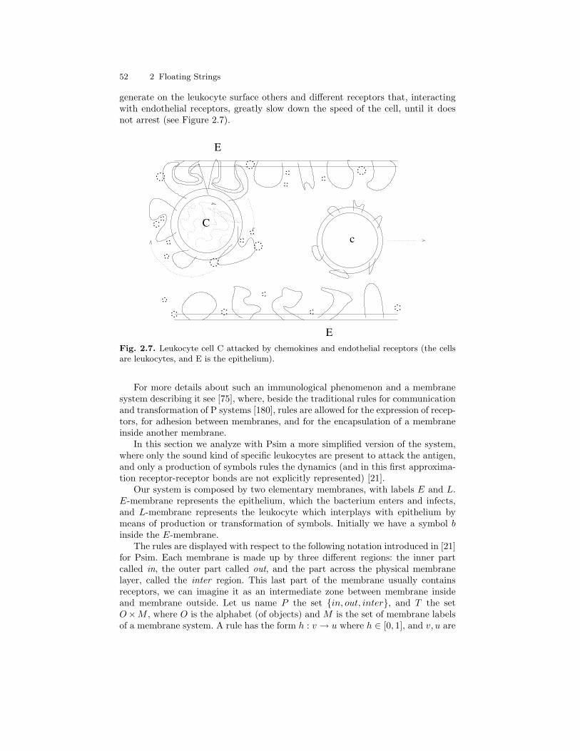
52 2 Floating Strings
generate on the leukocyte surface others and different receptors that, interactingwith endothelial receptors, greatly slow down the speed of the cell, until it doesnot arrest (see Figure 2.7).
E
E
Cc
Fig. 2.7. Leukocyte cell C attacked by chemokines and endothelial receptors (the cellsare leukocytes, and E is the epithelium).
For more details about such an immunological phenomenon and a membranesystem describing it see [75], where, beside the traditional rules for communicationand transformation of P systems [180], rules are allowed for the expression of recep-tors, for adhesion between membranes, and for the encapsulation of a membraneinside another membrane.
In this section we analyze with Psim a more simplified version of the system,where only the sound kind of specific leukocytes are present to attack the antigen,and only a production of symbols rules the dynamics (and in this first approxima-tion receptor-receptor bonds are not explicitly represented) [21].
Our system is composed by two elementary membranes, with labels E and L.E-membrane represents the epithelium, which the bacterium enters and infects,and L-membrane represents the leukocyte which interplays with epithelium bymeans of production or transformation of symbols. Initially we have a symbol binside the E-membrane.
The rules are displayed with respect to the following notation introduced in [21]for Psim. Each membrane is made up by three different regions: the inner partcalled in, the outer part called out, and the part across the physical membranelayer, called the inter region. This last part of the membrane usually containsreceptors, we can imagine it as an intermediate zone between membrane insideand membrane outside. Let us name P the set {in, out, inter}, and T the setO×M , where O is the alphabet (of objects) and M is the set of membrane labelsof a membrane system. A rule has the form h : v → u where h ∈ [0, 1], and v, u are

2.5 Membrane systems 53
strings over T ×P . Namely, k : (o,m, in)→ (o′,m′, out)(o′′,m′′, inter) means thatthe rule with reactivity k (that alters the uniform distribution of probability in theapplication of the rule), replaces the object o that is located inside the membranem, with the object o′ in the region external to the membrane m′ and with o′′ inthe intermediate location of the membrane m′′. In the following, for notationalconvenience, we write the string (cn,m, t) instead of the string (c,m, t)n, wherec ∈ O, m ∈M , t ∈ P , and n ∈ N.
The simple process we model is the following. The antigen inside the epithe-lium produces externally substances called chemokines together with epithelialreceptors, and internally copies of itself. Chemokines transform into internal sig-nals inside the leukocyte (this simulates the activation of the leukocytes). Theseinternal signals transform into leukocyte receptors in two steps. When a sufficientnumber of both epithelial and leukocyte receptors are present in the system, theelimination of bacterium is trigged by the production of a symbol v (this is anabstraction of the diapedesis phenomenon [75]).
We consider the alphabet {b, c, p, q1, q2, s, v}, and initially we have only thesymbol b, representing the replicating bacterium, inside the E-membrane:
k1 : (b, E, in)→ (bb, E, in).
During the process, b produces several symbols c (we fixed a rate of 3 copiesfor each copy of b), representing the chemokines, out of the membrane E, andmore symbols p (2 copies for each b), representing the epithelial receptors, on thesurface of E:
k2 : (b, E, in)→ (c3, E, out)(b, E, in)
k3 : (b, E, in)→ (p2, E, inter)(b, E, in).
The chemokines c out of the membranes transform into symbols s, represent-ing internal signals, inside L-membrane, and s is transformed in q2 (representingleukocyte receptors) ‘slowly’, that is by passing trough a transformation into 5copies of q1:
k4 : (c, E, out)→ (s, L, in)
k5 : (s, L, in)→ (q51 , L, inter)
k6 : (q1, L, inter)→ (q2, L, inter)
Finally, the presence in the system of both p and q2, representing epithelial andleukocyte receptors, actives the production of a symbol v inside the E-membrane,where each copy b is deleted by the presence of v:
k7 : (p,E, inter)(q2, L, inter)→ (v,E, in)
k8 : (b, E, in)(v,E, in)→ (v,E, in).
Given this system, the point was to regulate the values of the reactivitiesk1, . . . , k8 so that the application of the rules is modulated in the sound waywhich allows to neutralize the infection. As one can see in Figures 2.8 and 2.9,both taken from [21], once fixed k1 = 1, k2 = 1, k3 = 0.8, k4 = 0.7, k5 = 1,k6 = 0.2, k7 = 0.8, k8 = 1, the immune response works in a sound way in order todestroy all copies of a replicating b.

54 2 Floating Strings
Fig. 2.8. Patterns of bacterial infection (red) and leukocyte internal signals(blue). Quantities of b inside E and s inside L after 18 applications of the rules andwith a maximum capacity of membranes of 106.
In Figure 2.8 note how the decreasing of the infection (the quantity of b insideE) corresponds just to the increasing of the activation of leukocytes (quantity ofs inside L), as it is well known from immunological studies [216]. Also, when theinfection disappears then the production of s slows down quickly. Moreover, inFigure 2.9 one may see that the production of epithelial receptors is higher thanthe production of chemokines, while their behaviour following the pattern of b(infection) quantity, and this is confirmed from immunological studies as well [216].
For more details about the application strategy of the rules in each computa-tional step of the simulations, see [21].
The content of this chapter may be respectively found along parts of the follow-ing papers, sometimes with more details and sometimes by a different approach:
• G. F., V. Manca, An Algorithmic Analysis of DNA Structure (short version),Gh. Paun, C. Zandron, editors, Preliminary Proceedings of WMC 2002, Curteade Arges, Romania, August 19-23, pp 207–219, 2002.

2.5 Membrane systems 55
Fig. 2.9. Patterns of bacterial infection (red), chemokines (blue), and epithe-lial receptors (black). Respectively b, c, p quantities in: (top) 16 applications of therules and 106 as maximum capacity of membranes, (bottom) 19 applications of the rulesand 107 as maximum capacity of membranes.
• G. F., V. Manca, An Algorithmic Analysis of DNA Structure, Soft Computing,9(10), pp 761–768, October 2005.
56 2 Floating Strings
• G. F., M. Margenstern, Computing by Floating Strings, Proceedings of MeCBIC(Workshop on Membrane Computing and Biologically Inspired Process Cal-culi), Venice, Italy, July 9, 2006, ENTCS (Electronic Notes in TheoreticalComputer Science), submitted.
• G. F., V. Manca, A Membrane System for the Leukocyte Selective Recruitment,C. Martın-Vide, G. Mauri, Gh. Paun, G. Rozenberg, A. Salomaa, editors, Mem-brane Computing, Revised Papers of WMC 2003, LNCS 2933, Springer-Verlag,Heidelberg, Germany, pp 181-190, July 2004.
• L. Bianco, F. Fontana, G. F., V. Manca, P Systems for Biological Dynamics,Chapter 3 (invited) of G. Ciobanu, Gh. Paun, M. J. Perez-Jimenez, editors,Applications of Membrane Computing, Natural Computing Series, Springer,pp 83-128, 2006.

3
Cross Pairing PCR
We can see only a short distance ahead,but we can see plenty there that needs to be done.
Alan Mathison Turing1
The Polymerase Chain Reaction (PCR), which has allowed far more rapidamplification of DNA fragments than conventional molecular cloning, has beendescribed as “being to genes what Gutenberg’s printing press was to the writtenword”. The idea underlying its methodology is simple, but its impact has beenextraordinary. The first publication appeared in December 1985 [207], where thetechnique was used in an analysis of sickle cell anemia; a year later, the promiseimplicit in PCR amplification for large-scale sequencing efforts has been suggestedin [171,211], and every year thereafter, the number of papers on PCR has increasedtremendously [170]. In 1989, Science magazine selected PCR as the ‘major scientificdevelopment’ and Taq DNA Polymerase as the ‘molecule of the year’. In 1993, KaryMullis received the Nobel Prize for chemistry.
Because of PCR, ‘insufficient DNA’ has been no longer a limitation in molecularbiology research or DNA-based diagnostic procedures. In fact, the full benefits ofPCR in the emerging field of molecular diagnostic have yet to be realized [163].Given the low frequency of sequence errors observed in such a technique, thespeed and the sensitivity, several variants have been introduced, also for purposeof computation, such as whiplash PCR, whose idea was introduced in [210], andmore recent quantitative (real time) PCR [121] and emulsion PCR [53].
In Section 3.3 we present a special type of PCR, called Cross Pairing PCR2
(shortly XPCR), which was tested by laboratory experiments in several situations,all reported in Chapter 6. In fact, as the scientific methodology suggests, such atechnique had to pass inevitably through an iterative process involving a closeinteraction between experimentation and computation.
1 Computing machinery and intelligence. Mind, 59:433-460, 1950.2 Invention ‘Cross Pairing Polymerase Chain Reaction’ covered by a U.S. preliminary
patent from Department of Commerce, Docket number: BUCH-001PRV.
58 3 Cross Pairing PCR
As relevance of this method in the context of DNA computing, we show how itwas basic in the biotechnological procedures which implemented an algorithm forgenerating a complete n-bit library (Section 4.1), an algorithm for selecting thestrands containing a given substrand γ from an heterogeneous pool (Section 3.4),and an algorithm performing mutagenesis (Section 5.4). The experiments describedin Chapter 6 confirmed the correctness and completeness of the biomolecular algo-rithms proposed, and their implementation resulted to be convenient with respectto the standard methods, for efficiency, speed and feasibility.
In general and abstract terms, XPCR is a method for performing a transfor-mation on strings, that is essentially the splicing combinatorial mechanism in theoriginal formulation introduced by Tom Head in [97]; more precisely, it implementsa null context splicing rule (Definition 3.2). An analysis of PCR process besidesome notions related to splicing rules are given respectively in the next sectionsas background for the description of XPCR method and XPCR based algorithms.An extraction procedure based on XPCR technique is proposed in Section 3.4,whereas in Section 3.5 one can find both basic concepts about involution codes,and some encoding problems related to the experiments.
All the bio operations we are going to consider are performed in a test tubecontaining many copies of each DNA sequence. In the following we say pool Pthe content of such a test tube; formally it is a multiset of strings, which is a setof strings having positive multiplicity. The union operation P1 ∪P2 (also calledmerge) produces the pool resulting after a mix of the two pools P1 and P2.
There is a natural association between a DNA sequence and the number ofits bases, that number is called the length of the sequence. Electrophoresis is astandard gel-based technique that selects DNA sequences with respect to theirlength. Its precision depends on the kind of gel, and also sequences that differsof one basis can be separated (technical details are reported in Subsection 6.2.2).We denote by Elr(P) the pool obtained from P after an electrophoresis wherethe sequences r long were selected, or, in other words, the pool containing all thesequences of P having length exactly r.
3.1 PCR
The Polymerase Chain Reaction is one of the most important and efficient tool inbiotechnological manipulation and analysis of long DNA molecules. PCR exploitsthe remarkable natural function of the enzymes known as polymerases. These en-zymes are present in all living things, and their job is to copy genetic material.Sometimes referred to as ‘molecular photocopying’, PCR can characterize, ana-lyze, and synthesize any specific piece of DNA or RNA. It works even on extremelycomplicated mixtures, seeking out, identifying, and duplicating a particular bit ofgenetic material from blood, hair, or tissue specimens, from microbes, animals, orplants. The key to the process’s automation has been the Taq polymerase. Taq isa nickname for Thermus Aquaticus, a bacterium that happily survives and repro-duces in an environment that is lethal to other organisms: hot springs. That is whythe organism’s polymerase is perfectly at home in the rapidly fluctuating temper-atures of automated PCR. Unlike other polymerases, the enzyme extracted from

3.1 PCR 59
Taq (and now made in commercial quantities by genetically engineered bacteria)is stable at high temperatures. The microbiologists who found these remarkableorganisms decades ago, and then spent years studying their physiology and bio-chemistry, had no way of knowing how crucial their work would become to humanhealth, to the forensic sciences, and to the economy (Section 5.5). Who wouldhave thought a bacterium hanging out in a hot spring in Yellowstone NationalPark would spark a revolutionary new laboratory technique?
To copy DNA, polymerase requires two other components: a supply of the fournucleotide bases and an oligonucleotide called primer. DNA polymerases, whetherfrom humans, bacteria, or viruses, cannot copy a chain of DNA without a shortsequence of nucleotides to ‘prime’ the process, or get it started. In fact, the cellhas another enzyme called primase that actually makes the first few nucleotidesof the copy. Once the primer is made, the polymerase can take over making therest of the new chain. In fact, starting from the primer, the polymerase can read atemplate strand and match it with complementary nucleotides very quickly. Theresult is two new helices in place of the first, each composed of one of the originalstrands plus its newly assembled complementary strand3, as in Figure 3.1.
Fig. 3.1. Double helix ‘semiconservative’ autoduplication in the cell.
3 In nature, most organisms copy their DNA in the same way. When any cell divides,enzymes called polymerases make a copy of all the DNA in each chromosome. Thefirst step in this process is to ”unzip” the two DNA chains of the double helix. As thetwo strands separate, DNA polymerase makes a copy using each strand as a template(Figure 3.1). The PCR mimics this process, only it does it in a test tube and by usingonly a 5′-3′ writing polymerase.
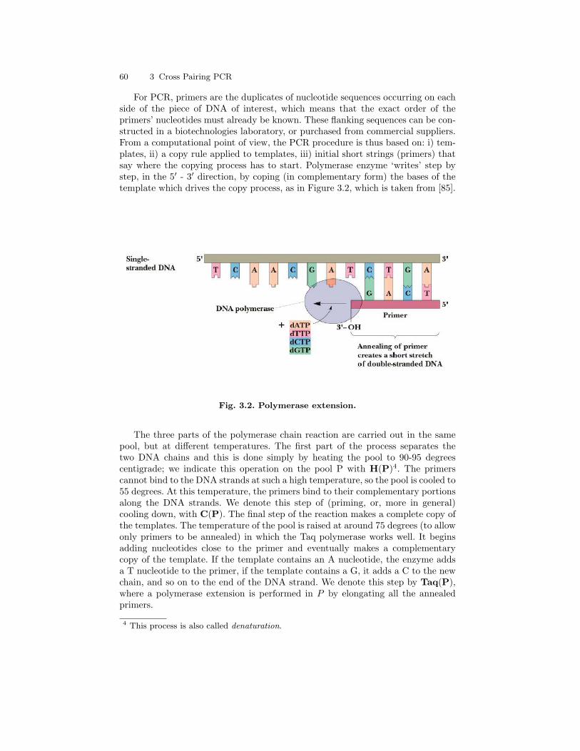
60 3 Cross Pairing PCR
For PCR, primers are the duplicates of nucleotide sequences occurring on eachside of the piece of DNA of interest, which means that the exact order of theprimers’ nucleotides must already be known. These flanking sequences can be con-structed in a biotechnologies laboratory, or purchased from commercial suppliers.From a computational point of view, the PCR procedure is thus based on: i) tem-plates, ii) a copy rule applied to templates, iii) initial short strings (primers) thatsay where the copying process has to start. Polymerase enzyme ‘writes’ step bystep, in the 5′ - 3′ direction, by coping (in complementary form) the bases of thetemplate which drives the copy process, as in Figure 3.2, which is taken from [85].
Fig. 3.2. Polymerase extension.
The three parts of the polymerase chain reaction are carried out in the samepool, but at different temperatures. The first part of the process separates thetwo DNA chains and this is done simply by heating the pool to 90-95 degreescentigrade; we indicate this operation on the pool P with H(P)4. The primerscannot bind to the DNA strands at such a high temperature, so the pool is cooled to55 degrees. At this temperature, the primers bind to their complementary portionsalong the DNA strands. We denote this step of (priming, or, more in general)cooling down, with C(P). The final step of the reaction makes a complete copy ofthe templates. The temperature of the pool is raised at around 75 degrees (to allowonly primers to be annealed) in which the Taq polymerase works well. It beginsadding nucleotides close to the primer and eventually makes a complementarycopy of the template. If the template contains an A nucleotide, the enzyme addsa T nucleotide to the primer, if the template contains a G, it adds a C to the newchain, and so on to the end of the DNA strand. We denote this step by Taq(P),where a polymerase extension is performed in P by elongating all the annealedprimers.
4 This process is also called denaturation.
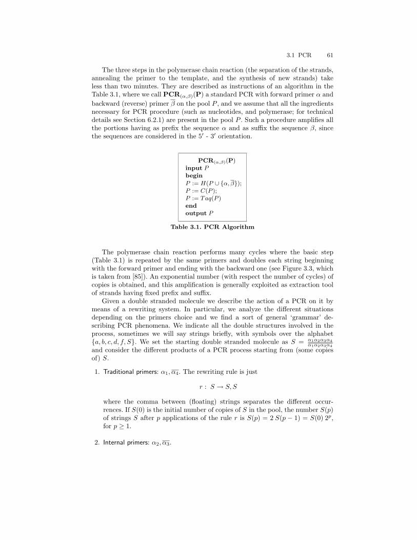
3.1 PCR 61
The three steps in the polymerase chain reaction (the separation of the strands,annealing the primer to the template, and the synthesis of new strands) takeless than two minutes. They are described as instructions of an algorithm in theTable 3.1, where we call PCR(α,β)(P) a standard PCR with forward primer α andbackward (reverse) primer β on the pool P , and we assume that all the ingredientsnecessary for PCR procedure (such as nucleotides, and polymerase; for technicaldetails see Section 6.2.1) are present in the pool P . Such a procedure amplifies allthe portions having as prefix the sequence α and as suffix the sequence β, sincethe sequences are considered in the 5′ - 3′ orientation.
PCR(α,β)(P)input Pbegin
P := H(P ∪ {α, β});P := C(P );P := Taq(P )endoutput P
Table 3.1. PCR Algorithm
The polymerase chain reaction performs many cycles where the basic step(Table 3.1) is repeated by the same primers and doubles each string beginningwith the forward primer and ending with the backward one (see Figure 3.3, whichis taken from [85]). An exponential number (with respect the number of cycles) ofcopies is obtained, and this amplification is generally exploited as extraction toolof strands having fixed prefix and suffix.
Given a double stranded molecule we describe the action of a PCR on it bymeans of a rewriting system. In particular, we analyze the different situationsdepending on the primers choice and we find a sort of general ‘grammar’ de-scribing PCR phenomena. We indicate all the double structures involved in theprocess, sometimes we will say strings briefly, with symbols over the alphabet{a, b, c, d, f, S}. We set the starting double stranded molecule as S = α1α2α3α4
α1α2α3α4and consider the different products of a PCR process starting from (some copiesof) S.
1. Traditional primers: α1, α4. The rewriting rule is just
r : S → S, S
where the comma between (floating) strings separates the different occur-rences. If S(0) is the initial number of copies of S in the pool, the number S(p)of strings S after p applications of the rule r is S(p) = 2 S(p − 1) = S(0) 2p,for p ≥ 1.
2. Internal primers: α2, α3.

62 3 Cross Pairing PCR
Fig. 3.3. PCR amplification.
If we set a = α1α2α3α4α1α2α3
, b = α2α3α1α2α3
, c = α2α3α2α3
, d = α2α3α4α2α3
, f = α2α3α4α1α2α3α4
,then the rewriting rules miming the PCR process with internal primers are
S → a, fa → a, bb → c, bc → c, cd → c, df → f, d.

3.1 PCR 63
We assume that initially in the pool there are only copies of S, that isa(0) = b(0) = c(0) = d(0) = e(0) = f(0) = 0. Note that S disappears as soonas the process starts, the symbols a and f maintain a constant quantity equal toS(0) after their generation in the first step: a(p) = a(1) = S(0) = f(1) = f(p)with p ≥ 1, the amount of symbols b and d increases linearly with the numberof steps: b(p) = (p − 1) a(1) = (p − 1) f(1) = d(p) for p ≥ 1, and the doublestructure c is the amplified product. The increasing of its quantity can be writ-ten recursively as c(p) = b(p− 1) 2 + c(p− 1) 2, where the first term measuresthe production from the symbols b and d present in the previous step, and thesecond term quantifies the production from symbols c themselves.
3. Traditional and internal primers: α1, α3 (the case α2, α4 is analogous: in thesystem rules the symbol f would be replaced by a. Let c = α2α3α4
α2α3α4).
In a sense, it is a simplified version of the previous system, because only fromone (untraditional) primer the linear production is allowed.S → S, a
a → a, cc → c, c
where a = α1α2α3α4α1α2α3
and c = α1α2α3α1α2α3
. As consequence of the traditionalprimer action S(p) = S(0) for p ∈ N, therefore a(p) = S(0) p. Whereasc(p) = a(p− 1) + 2c(p− 1) with p ≥ 1.
4. External primers: α0α1, α4α5, leads a system analogous to the second case (withinternal primers).
S → a, fa → a, bb → c, bc → c, cd → c, df → f, d
where the symbols are analogously set as a = α1α2α3α4α1α2α3α4α5
, b = α0α1α2α3α4α5α1α2α3α4α5
,c = α0α1α2α3α4α5
α0α1α2α3α4α5, d = α0α1α2α3α4
α0α1α2α3α4α5, f = α0α1α2α3α4
α1α2α3α4.
5. Traditional and external primers: α1, α4α5, leads to a system analogous to thethird case.
In conclusion, a general PCR process amplifies portions of double strandedmolecules, even elongating them by means of external primers. When un-tradi-tional primers are used, then exponential amplification starts only after some stepsand linear products are added in the pool. As a consequence, PCR process requiresmore material consumption and space occupation than in the standard case.
From a formal language theory viewpoint, the following system describes thewhole process (see Figure 3.4):

64 3 Cross Pairing PCR
S → a, fa → a, bb → c, bc → c, cd → c, df → f, d
where every rule applies on an element, and replaces it with two elements, but thereis no generation of languages. In fact, during the process the set of string-objectseither remains {S}, by traditional primers, or remains {a, b, c, d, f} after a fist step,where the symbol S has disappeared). Rather, the multiplicity associated to eachobject changes in each step, as often it happens in membrane computing, and thestudy of such dynamics is useful to analyze the amount of desired or redundantPCR products in the pool. This analysis would be useful in DNA computing,where the amount of DNA is a strict limit for the scale-up of many procedures.There exists a recent variant of PCR, called Real Time PCR [121], that measuresthe amount of amplified DNA. By such a method, the quantity of amplificationis detected by a fluorescence added to the primers together with a quencher; itis released during the Taq polymerase extension so that finally the fluorescenceresults proportional to the amplified material.
S
a f
af
b d
c c
cc
cc
b
cc c c c c c
ab b
bc
fd
cc
c c
d
ccc
d
dc
Fig. 3.4. PCR process.
As pointed out in [235], in the algorithms based on PCR one has to keep in mindthat a restricted number of PCR operations are possible before to reach the limitof DNA quantity we can handle in a test tube. In our algorithms and experimentsthis information was considered in any step, and electrophoresis usually selectedparts of previous amplifications.

3.1 PCR 65
3.1.1 PCR variants
In literature there exist many different variants of PCR. As examples we considerWhiplash PCR, that has been used as computational tool in [94,210,236,134,197],and Emulsion PCR [91, 53], that has been exploited for very recent sequencingtechnologies in [219].
Whiplash PCR originally used a single molecule and its hairpin formation toimplement a finite state machine by polymerase extension [94], and then it wascombined with combinatorial assembly PCR to generate structured libraries andto solve several NP-complete problems in a constant number of biosteps [236].WPCR utilizes the facts that a single stranded DNA can anneal to a portion ofitself (by forming a hairpin structure) and that polymerase extension can performa task of reading out data written on the DNA sequence itself. The single strandedmolecule is composed by an input segment on the 5′-end, followed by a µ-formula(a boolean formula with each variable occurring once) segment (program), followedby a spacer, and finally by a ‘head’ on the 3′-end that moves and performs thecomputation. The head anneals to complementary subsequences in the input andformula alternatively, exactly in the same way the transitions were implementedin [210], where the change from a statei to the next state state′i of an automatonwas described as in Figure 3.5.
, ,
,,
, ,
i i j j
i
i i j j
j i
i i j j
jstate
state state state state
state
j = state state state
state state
state state
state state state state
Fig. 3.5. Current statei is attached to form an hairpin structure and its extension isperformed by polymerase action. After denaturation the computation advances with thenew current statej at the 3′-end.
On the experimental front, in [94] was demonstrated how to perform the poly-merization stop reaction, and two successive head transitions of a very simple ver-sion of (very short) self-acting molecule were observed, but little is known aboutthe capability of whiplash to perform computations in practice. In fact, from the

66 3 Cross Pairing PCR
point of view of DNA Computing, Whiplash PCR is a nice model of computationwith the advantage of performing single-tube computation of many programs inparallel, but it faces serious problems and limitations that need to be addressedexperimentally.
An obvious question is how large a single-stranded molecule can be, and howlonger it can grow during the computation without breaking. The answer couldpose limits on the size of problems that the method can handle. A more sever prob-lem would be generated by formations of loops in different parts of the sequence.Another critical problem is the possibility of different molecules interacting. Inparticular, it is necessary to determine at what concentration molecules start tointeract with each other at a significant frequency (forming aggregates observablein the gel) and how these interactions scale with the size and number of moleculesused. Allowable levels of concentration in order to minimize interactions could verylikely be dependent on the size of molecules. They should be investigated so thatthe crucial volume requirements of the method could be determined.
Recent progress in WPCR techniques can be found in [134] where implemen-tation of input/output interface and the multiple transition steps on solid phaseare reported. In fact, in the implementation of WPCR with I/O interface, it is ofgreat importance to keep the independence of each molecular machine, but at thesame time it is also necessary to prevent an intermolecular reaction, and this wasdone by adopting a solid phase method [243].
In PNA-mediated Whiplash PCR (PWPCR) [196], an autonomous molecularcomputation is implemented by the recursive polymerase extension of a mixtureof DNA hairpins. Like other methods based on exhaustive search, however, appli-cation to problem instances of realistic size is prevented by the exponential scalingof the solution space. The tendency of evolving populations to minimize the sam-pling of large, low fitness basins suggests that a DNA-based evolutionary approachmight be an effective alternative to exhaustive search, and in [197] PWPCR hasbeen modified to support the evolution of a population of finite state machines.Moreover, an in vitro algorithm for applying this architecture to evolve approxi-mate solutions to instances of NP-complete problems, such as Hamiltonian Paths,is described in detail.
Together with in situ rolling circle amplification (RCA), bridge polymerasechain reaction [145] and picotiter PCR, Emulsion PCR is a technology performingmultiplex amplification while maintaining spatial clustering of identical moleculesto amplify. An optimized version of it has used to robustly and reproducibly am-plify complex libraries for a new low-cost and rapid DNA sequencing technol-ogy [219]. Such a technique is the actual implementation of a membrane systemwith many elementary membranes (inside the skin membrane representing the testtube) where different PCRs are carried on.
The idea underlying the Emulsion PCR was introduced in [226], and the tech-nique was then improved in [91], where a compartmentalized selfreplication reac-tion (CSR) was suggested as a strategy to isolate individual polymerase variantsin separate compartments, in order to select polymerases with novel and usefulproperties. Provided that in each compartment one has genes and correspondingprimers, each modified polymerase replicates only its own encoding gene to theexclusion of those in other compartments. Consequently, only genes encoding ac-

3.1 PCR 67
tive polymerases are replicated, whereas inactive variants fail to amplify their owngenes. Among differentially active variants, the more active can be expected toproduce proportionally more ‘offspring’. Such reactions took place in individualaqueous compartments of a water-in-oil emulsion that are stable for prolongedperiods at temperatures exceeding 90◦C. A water-in-oil emulsion permits millionsof noninteracting amplifications within a milliliter-scale volume.
Compartments have average diameters of 15 µm and they are proved to beheat-stable. Once formed, they do not permit exchange of macromolecules likeDNA or protein. Presumably, their large molecular weight and electric chargeprevent their diffusion across the droplets surface, even at high temperatures,and the droplets work as microreactors [91]. Small molecules instead, includingthe negatively charged dNTP (free nucleotides necessary to perform PCRs), cancross the surfaces and stay between the compartments during thermocycling. Byincreasing the oil-in-water ratio of the emulsion though, dNTP diffusion could becontrolled [91], and in general, controlled communication between compartmentsoffers prospects for the extension of CSR technology, while the model seeming tofit exactly a membrane system.
Emulsion PCR was used in [53] as extraction method, to detect a certain stringin an initial population of DNA molecules, and to quantify the fraction of somekind of DNA molecules in that population. Such a technique resulted successful toanalyze a large number of molecules independently while retaining a high signal-to-noise ratio. Amplification products of individual compartments in [53, 219] arecaptured via inclusion of 1-µm paramagnetic beads bearing one of the PCR primers(beads having been previously coated with streptavidin and bound to biotinylatedoligonucleotides). Any single bead bears thousands of single-stranded copies ofthe same PCR product, whereas different beads bear the products of differentcompartmentalized PCR reactions (see Figure 3.6, which is taken from [219]).
Increasing template concentration in an emulsion PCR reaction boosts the frac-tion of amplified beads at the cost of greater non-clonality. The beads generated byemulsion PCR have highly desirable characteristics: high signal density, geometricuniformity, strong feature separation, and a size that is small but still resolvableby inexpensive optics.
Fig. 3.6. An aqueous mix containing all the necessary components for PCR plus primer-bound beads and template DNA are stirred together with an oil/detergent mix to createmicroemulsions. The microemulsions are temperature-cycled as in a conventional PCR.If a DNA template and a bead are present together in a single aqueous compartment,the bead-bound oligos act as primers for amplification.
68 3 Cross Pairing PCR
This is a quite sophisticated and still experimental technique, even because theuse of beads requires very specialized instruments and laboratories. In Section 3.3we propose another variant of the PCR technique, but before to get under waylet us review the theoretical context of the splicing rules, since it implements aparticular combinatorial rule called null context splicing.
3.2 Splicing rules
The splicing systems proposed by Head in [97] represent a significant body ofliterature; we recall here some definitions as introduced originally.
Over a finite alphabet A, a rule set R is a set of strings p#q$u#v where p, q, u, vare strings of A? and #, $ special symbols. The combination of an initial languageI contained in A? with a rule set R yields a splicing system G = (A, I,R). Thistriple is regarded as a formal device, inspired by cut and paste phenomena on DNAmolecules under the action of restriction and ligase enzymes, that generates fromI a language L(G) that is defined recursively. L(G) is the smallest language in A?
that contains I and has the following closure property with respect to R: for eachpair of strings wpqx and yuvz in L(G), where w, x, y, z are in A? and p#q$u#v inR, wpvz is also in L(G), and we say that it is obtained by splicing from the twostrings.
Definition 3.1. A language L is said to be a splicing language if there exists asplicing system G = (A, I,R) for which L = L(G).
An element p#q$u#v of the rule set is called splicing rule and it recombinestwo strings along the two different sites p#q and u#v as it follows:
w p q x, y u v z −→ w p v z
A “symmetric” version of such a rule produces both the strings wpvz and yuqxwhen applied on wpqx and yuvz. The symmetric splicing rules model the behaviourof enzymes that cut and glue DNA molecules. In fact, the restriction enzymes willbind to DNA at a specific recognition site and then cleave DNA mostly within, butsometimes outside, of this recognition site, while the ligase enzymes glue togethertwo molecules wherever it finds nicks between symbol-nucleotides, as in Figure 3.7which is taken from [69]. This type of cut and paste activity provides the basis forthe technology of gene splicing [99].
Finite splicing systems are those having only finitely many rules and finitelymany initial strings. Languages generated by such systems are necessarily regular,but not all regular languages can be so generated [146,147]. These systems generatejust a restricted subclass of the class of regular languages [103], for example, theyare not able to generate the regular languages a∗ba∗ba∗ and (aa)∗.
If one considers particular splicing rules p#q$u#v where (namely) p = u andqv = λ, then one obtains the following kind of rule, also called one sided contextbecause tests context on only one side [99].
Definition 3.2. The null context splicing rules are of type
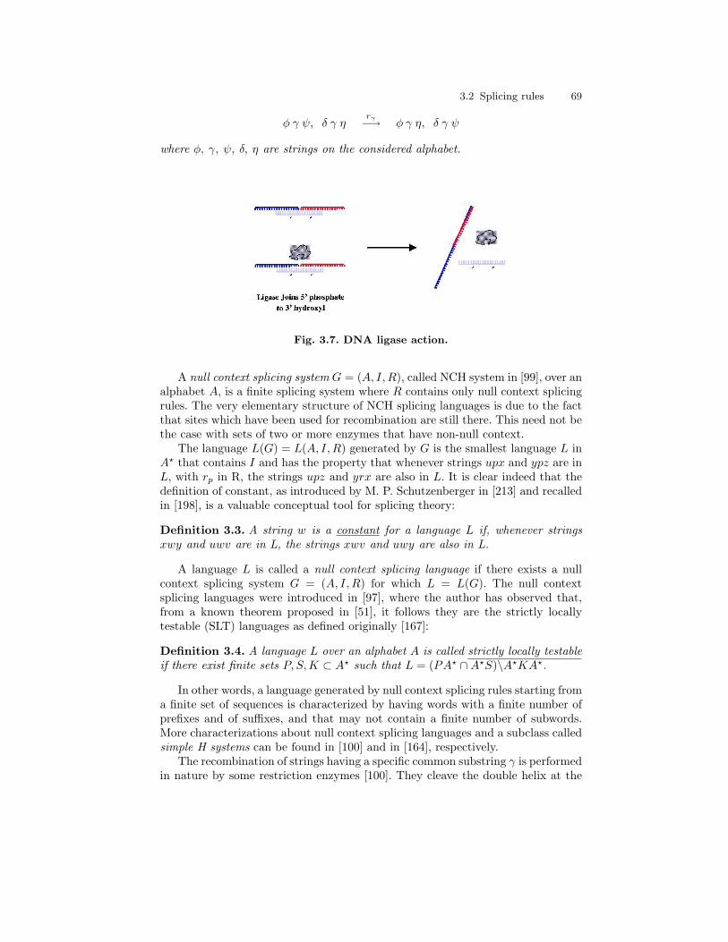
3.2 Splicing rules 69
φ γ ψ, δ γ ηrγ−→ φ γ η, δ γ ψ
where φ, γ, ψ, δ, η are strings on the considered alphabet.
Fig. 3.7. DNA ligase action.
A null context splicing system G = (A, I,R), called NCH system in [99], over analphabet A, is a finite splicing system where R contains only null context splicingrules. The very elementary structure of NCH splicing languages is due to the factthat sites which have been used for recombination are still there. This need not bethe case with sets of two or more enzymes that have non-null context.
The language L(G) = L(A, I,R) generated by G is the smallest language L inA? that contains I and has the property that whenever strings upx and ypz are inL, with rp in R, the strings upz and yrx are also in L. It is clear indeed that thedefinition of constant, as introduced by M. P. Schutzenberger in [213] and recalledin [198], is a valuable conceptual tool for splicing theory:
Definition 3.3. A string w is a constant for a language L if, whenever stringsxwy and uwv are in L, the strings xwv and uwy are also in L.
A language L is called a null context splicing language if there exists a nullcontext splicing system G = (A, I,R) for which L = L(G). The null contextsplicing languages were introduced in [97], where the author has observed that,from a known theorem proposed in [51], it follows they are the strictly locallytestable (SLT) languages as defined originally [167]:
Definition 3.4. A language L over an alphabet A is called strictly locally testableif there exist finite sets P, S,K ⊂ A? such that L = (PA? ∩A?S)\A?KA?.
In other words, a language generated by null context splicing rules starting froma finite set of sequences is characterized by having words with a finite number ofprefixes and of suffixes, and that may not contain a finite number of subwords.More characterizations about null context splicing languages and a subclass calledsimple H systems can be found in [100] and in [164], respectively.
The recombination of strings having a specific common substring γ is performedin nature by some restriction enzymes [100]. They cleave the double helix at the
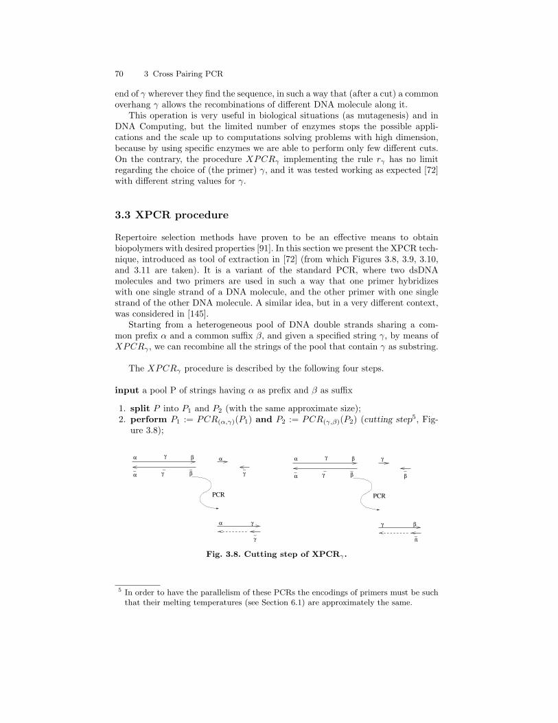
70 3 Cross Pairing PCR
end of γ wherever they find the sequence, in such a way that (after a cut) a commonoverhang γ allows the recombinations of different DNA molecule along it.
This operation is very useful in biological situations (as mutagenesis) and inDNA Computing, but the limited number of enzymes stops the possible appli-cations and the scale up to computations solving problems with high dimension,because by using specific enzymes we are able to perform only few different cuts.On the contrary, the procedure XPCRγ implementing the rule rγ has no limitregarding the choice of (the primer) γ, and it was tested working as expected [72]with different string values for γ.
3.3 XPCR procedure
Repertoire selection methods have proven to be an effective means to obtainbiopolymers with desired properties [91]. In this section we present the XPCR tech-nique, introduced as tool of extraction in [72] (from which Figures 3.8, 3.9, 3.10,and 3.11 are taken). It is a variant of the standard PCR, where two dsDNAmolecules and two primers are used in such a way that one primer hybridizeswith one single strand of a DNA molecule, and the other primer with one singlestrand of the other DNA molecule. A similar idea, but in a very different context,was considered in [145].
Starting from a heterogeneous pool of DNA double strands sharing a com-mon prefix α and a common suffix β, and given a specified string γ, by means ofXPCRγ , we can recombine all the strings of the pool that contain γ as substring.
The XPCRγ procedure is described by the following four steps.
input a pool P of strings having α as prefix and β as suffix
1. split P into P1 and P2 (with the same approximate size);2. perform P1 := PCR(α,γ)(P1) and P2 := PCR(γ,β)(P2) (cutting step5, Fig-
ure 3.8);
PCR
α γ β α
α γ
_ _ _ _
_
α γ β
γ
γ
α γ β
_ _ _ _
_
α γ β
PCR
γ
β
γ β
β
Fig. 3.8. Cutting step of XPCRγ .
5 In order to have the parallelism of these PCRs the encodings of primers must be suchthat their melting temperatures (see Section 6.1) are approximately the same.
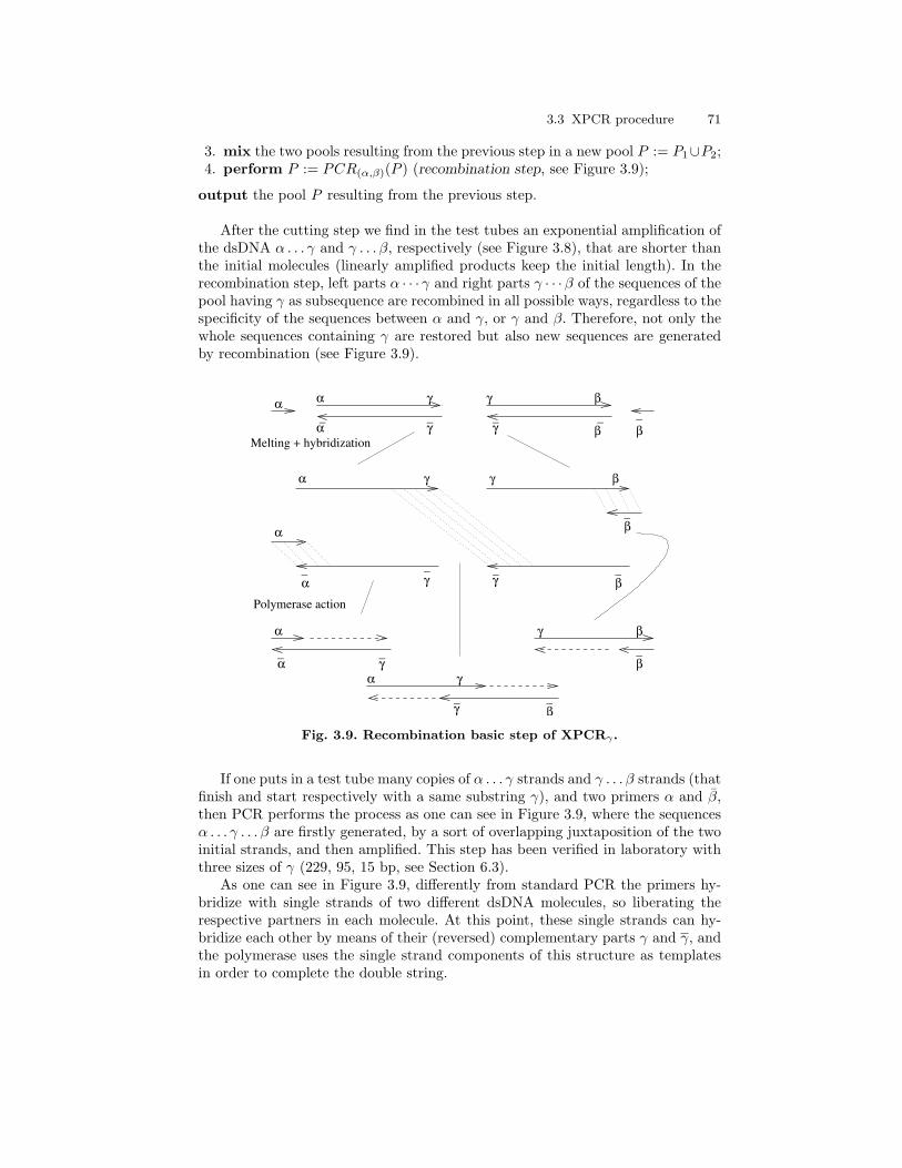
3.3 XPCR procedure 71
3. mix the two pools resulting from the previous step in a new pool P := P1∪P2;4. perform P := PCR(α,β)(P ) (recombination step, see Figure 3.9);
output the pool P resulting from the previous step.
After the cutting step we find in the test tubes an exponential amplification ofthe dsDNA α . . . γ and γ . . . β, respectively (see Figure 3.8), that are shorter thanthe initial molecules (linearly amplified products keep the initial length). In therecombination step, left parts α · · · γ and right parts γ · · ·β of the sequences of thepool having γ as subsequence are recombined in all possible ways, regardless to thespecificity of the sequences between α and γ, or γ and β. Therefore, not only thewhole sequences containing γ are restored but also new sequences are generatedby recombination (see Figure 3.9).
α γ γ βα _β
α
α γ γ β
α γ β
α γ
_ _ _ _
_
_ _ _ _
_ _ _
_ _
α γ γ β
β
α γ γ β
β
γ β
α γ
Melting + hybridization
Polymerase action
Fig. 3.9. Recombination basic step of XPCRγ .
If one puts in a test tube many copies of α . . . γ strands and γ . . . β strands (thatfinish and start respectively with a same substring γ), and two primers α and β,then PCR performs the process as one can see in Figure 3.9, where the sequencesα . . . γ . . . β are firstly generated, by a sort of overlapping juxtaposition of the twoinitial strands, and then amplified. This step has been verified in laboratory withthree sizes of γ (229, 95, 15 bp, see Section 6.3).
As one can see in Figure 3.9, differently from standard PCR the primers hy-bridize with single strands of two different dsDNA molecules, so liberating therespective partners in each molecule. At this point, these single strands can hy-bridize each other by means of their (reversed) complementary parts γ and γ, andthe polymerase uses the single strand components of this structure as templatesin order to complete the double string.
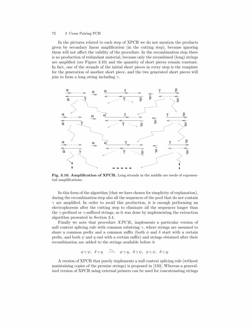
72 3 Cross Pairing PCR
In the pictures related to each step of XPCR we do not mention the productsgiven by secondary linear amplification (in the cutting step), because ignoringthem will not affect the validity of the procedure. In the recombination step thereis no production of redundant material, because only the recombined (long) stringsare amplified (see Figure 3.10) and the quantity of short pieces remain constant.In fact, one of the strands of the initial short pieces in every step is the templatefor the generation of another short piece, and the two generated short pieces willjoin to form a long string including γ.
α
α γ_ _ _
β
α_α γ
α
α_
γ
_
_
α
α γ_γ
_β β
_βγ
_β _
β
β_
β_
_β
γ
γ
β
β_β
_γ
γ_
α γ
α
α α γ
Fig. 3.10. Amplification of XPCR. Long strands in the middle are seeds of exponen-tial amplifications.
In this form of the algorithm (that we have chosen for simplicity of explanation),during the recombination step also all the sequences of the pool that do not containγ are amplified. In order to avoid this production, it is enough performing anelectrophoresis after the cutting step to eliminate all the sequences longer thanthe γ-prefixed or γ-suffixed strings, as it was done by implementing the extractionalgorithm presented in Section 3.4.
Finally we note that procedure XPCRγ implements a particular version ofnull context splicing rule with common substring γ, where strings are assumed toshare a common prefix and a common suffix (both φ and δ start with a certainprefix, and both ψ and η end with a certain suffix) and strings obtained after theirrecombination are added to the strings available before it
φ γ ψ, δ γ ηrγ−→ φ γ η, δ γ ψ, φ γ ψ, δ γ η.
A version of XPCR that purely implements a null context splicing rule (withoutmaintaining copies of the premise strings) is proposed in [150]. Whereas a general-ized version of XPCR using external primers can be used for concatenating strings

3.4 An extraction algorithm 73
in the following way. Suppose to have a pool P1 of strings having prefix α and suffixξ, and a pool P2 of strings having prefix ζ and suffix β. Given a (primer) string γ,we can generate a kind of language concatenation P1γP2 = {δγη | δ ∈ P1, η ∈ P2}with the algorithm in Table 3.2. If ξ = ζ, then P1P2 is obtained simply performingPCR(α,β)(P1 ∪ P2), that is the recombination step of XPCRξ.
P1 := PCR(α,ξγ)(P1) and P2 := PCR(γζ,β)(P2);
P1γP2 := PCR(α,β)(P1 ∪ P2).
Table 3.2. Concatenating by PCR
A differently arranged concatenation of sequences by XPCR was introducedand tested experimentally in [150].
3.4 An extraction algorithm
The extraction of DNA strands including a given sequence of bases is a crucial stepin both DNA computing and biotechnology. The extraction step of the Adleman-Lipton paradigm remains its critical point. The initial methods used membranefilters for separating by Watson-Crick complementarity the strands containinggiven substrands from the other ones. With a similar strategy the biotin-avidinaffinity allowed to select some strands by means of the complementary substrandsbond to beads, and this method had efficiency 88±3% [123]. In particular, as it isreported in [141], if we call p the percentage of sound extractions (extracting eachof the required DNA strands is equally likely) and we assume that for each distinctstring s in a test tube there are 10l (l = 13 proposed by Adleman in [1]) copies ofs, then no matter how large l is and no matter how close to 1 p is, there alwaysexists a class of 3-SAT problems such that DNA computing error must occur.
An alternative extracting method used hairpin formations of single strands astest of inconsistent assignments of variables [209], and this kind of computationwas combined with Whiplash PCR for simulating finite state machine [94]. Morerecently, microfluid devices for separating strands were introduced in [228], andan automated mix of thermocycler and gel-electrophoresis was developed in [28]in order to extract the strands encoding the satisfying assignments of a formulafrom a large pool of molecules. Finally, the idea of using PCR as a “very elegantand effective detection method” to check the existence of a solution was consid-ered in [203], where a theoretic method ‘blocking’ the wrong sequences with PNAstrands is proposed.
We address the following problem: given a specified sequence γ of bases, andan input pool P of different dsDNA molecules with a same length and sharing acommon prefix and suffix, we want to produce an output pool P ′ where only thestrands which include the given sequence γ are represented. Here we present an
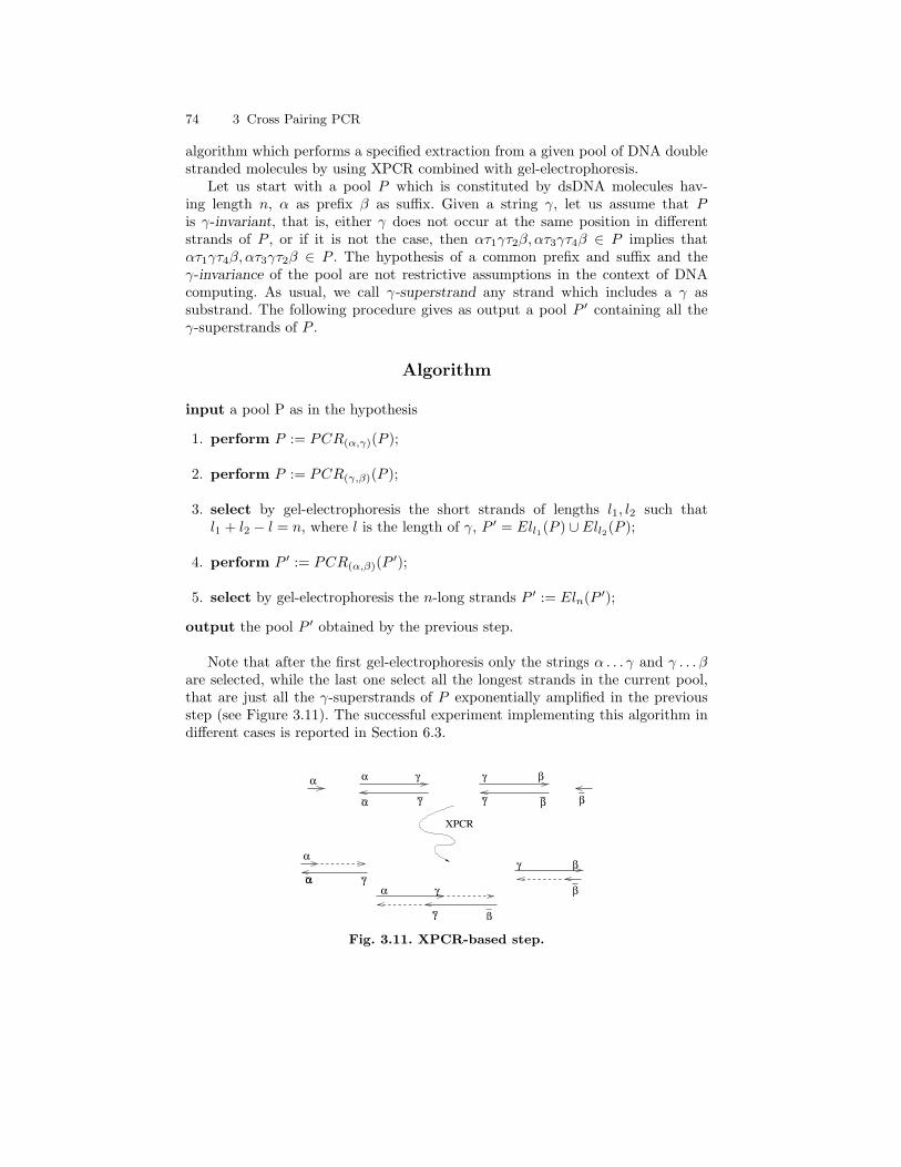
74 3 Cross Pairing PCR
algorithm which performs a specified extraction from a given pool of DNA doublestranded molecules by using XPCR combined with gel-electrophoresis.
Let us start with a pool P which is constituted by dsDNA molecules hav-ing length n, α as prefix β as suffix. Given a string γ, let us assume that Pis γ-invariant, that is, either γ does not occur at the same position in differentstrands of P , or if it is not the case, then ατ1γτ2β, ατ3γτ4β ∈ P implies thatατ1γτ4β, ατ3γτ2β ∈ P . The hypothesis of a common prefix and suffix and theγ-invariance of the pool are not restrictive assumptions in the context of DNAcomputing. As usual, we call γ-superstrand any strand which includes a γ assubstrand. The following procedure gives as output a pool P ′ containing all theγ-superstrands of P .
Algorithm
input a pool P as in the hypothesis
1. perform P := PCR(α,γ)(P );
2. perform P := PCR(γ,β)(P );
3. select by gel-electrophoresis the short strands of lengths l1, l2 such thatl1 + l2 − l = n, where l is the length of γ, P ′ = Ell1(P ) ∪ Ell2(P );
4. perform P ′ := PCR(α,β)(P ′);
5. select by gel-electrophoresis the n-long strands P ′ := Eln(P ′);
output the pool P ′ obtained by the previous step.
Note that after the first gel-electrophoresis only the strings α . . . γ and γ . . . βare selected, while the last one select all the longest strands in the current pool,that are just all the γ-superstrands of P exponentially amplified in the previousstep (see Figure 3.11). The successful experiment implementing this algorithm indifferent cases is reported in Section 6.3.
XPCR
α α γ γ β
α γ
_ _ _ _
_
α γ γ β
γ β
β_γ
_β
_β
_ _γ
α
αα
Fig. 3.11. XPCR-based step.

3.5 DNA involution codes 75
The advantage of XPCR based extraction method with respect to methodsfrom literature is that it is rapid, cheap, and easy to implement. In fact, it re-quires only PCR and electrophoresis techniques, both standard and very efficientmethodologies. On the other hand, as a disadvantage we point out its sensitivity,in the sense that any occasional error would be exponentially amplified. That is,with this procedure it is easier to find false positive than false negative.
In principle, operations as consecutive DNA extraction from a given pool bymeans of XPCR should work correctly, but problems could arise if the encoding isnot robust enough for avoiding unexpected annealing. In order to avoid undesirablehybridizations between words the language involved by the DNA operations hasto satisfy certain coding properties, and this is a requirement to investigate beforeany experiment. In fact, DNA strand design is one of the hardest subdisciplines ofDNA computing.
3.5 DNA involution codes
The computation language of a DNA-based system consists of all the words (DNAstrands) that can appear in any computation step of the system. Common ap-proach to avoid undesired intermolecular and intra-molecular hybridizations hasbeen to use the Hamming distance as a measure for uniqueness of strands [214].Also, theoretical methods for constructing coded DNA languages were investi-gated [114] and decidability of desired properties were addressed as well [106].
We give an overview of the main characterizations of involution codes, as prop-erties which ensure that the words in these languages will not form undesirablebonds when used in DNA computations. Given an involution h : Σ? → Σ? overa finite alphabet Σ, the involution codes h-infix, h-comma-free and h-k-codesintended for avoiding intermolecular hybridizations, and h-subword-k-codes in-tended for avoiding intra-molecular hybridizations, are presented in the following.
An involution h is a mapping such that h2 equals the identity mapping, thus itis bijective and h = h−1. It is called morphic if it is a morphism, and antimorphicwhen h(uv) = h(v)h(u) for any strings u, v on the given alphabet. A code X isa subset of Σ+ satisfying the property that, for every word w ∈ X+, there isa unique sequence v1, v2, . . . , vn of words in X such that w = v1v2 · · · vn. Thefollowing definitions are basic in the study of DNA coded languages, where X isa finite code and h : X? → X? is a morphic or antimorphic involution.
Definition 3.5. X is h-infix if A?h(X)A+ ∩X = ∅ and A?h(X)A+ ∩X = ∅.
In other words, if X is a h-infix involution code, an element of h(X) may not bea proper substring of an other element of X (see Figure 3.12). A stronger conditionfor X is the constraint to be an h-comma-free code.
Definition 3.6. X is h-comma-free if X2 ∩A+h(X)A+ = ∅.
In fact, by contradiction, if an element of h(X) is a proper substring of anotherone in X, then it is going to be an element of X2 ∩A+h(X)A+. Conversely, overthe alphabet {a, b}, the h-infix involution code X = {ab} with h(a) = b is not

76 3 Cross Pairing PCR
h-comma-free. In fact, X2 = {abab} and h(X) = {ba}, therefore the h-comma-freedom is a strictly stronger condition. On the other hand, h-infix codes are closedunder arbitrary concatenation while h-comma-free codes do not.
Intermolecular hybridizations
h−comma−free
h−infix
h−k−codes
Fig. 3.12. Forbidden cases for h-infix, h-comma free, and h-k-codes.
In this chapter we have used languages X with words of a fixed equal length.They are ‘almost’ h-infix, in the sense that it holds X2 ∩ A+h(X2)A+ = ∅ (seeLemma 1 in [113]).
To present a last property avoiding the intermolecular hybridization we recallthat Subk(X) is the set of all the k long subword of words in X.
Definition 3.7. X is h-k-code if for some k > 0 Subk(X) ∩ Subk(h(X)) = ∅.
All the forbidden cases of the above involution codes inspired by the problemsarising from the intermolecular hybridizations are illustrated in Figure 3.12.
The intra-molecular hybridizations generating (undesired) hairpin formationsare not a minor problem for DNA computations, and different versions of involutioncodes were defined to avoid them. The point is bounding in a suitable way thelength of the portions complementary to each other lying on a sequence and theirdistance along the sequence, see Figure 3.13.
Definition 3.8. For all sequences u ∈ A?, X is a
• h-subword-k-code if, for |u| = k and i ≥ 1, A?uAih(u)A? ∩X = ∅• h-subword-k −m-code if, for |u| = k and 1 ≤ i ≤ m, A?uAih(u)A? ∩X = ∅• h(k,m1,m2)-subword-complaint code if, for |u| > k and m1 ≤ m ≤ m2,
A?uAmh(u)A? ∩X = ∅.
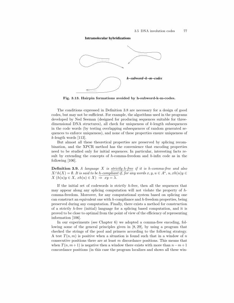
3.5 DNA involution codes 77
Intramolecular hybridizations
h−subword−k−m−codes
Fig. 3.13. Hairpin formations avoided by h-subword-k-m-codes.
The conditions expressed in Definition 3.8 are necessary for a design of goodcodes, but may not be sufficient. For example, the algorithms used in the programsdeveloped by Ned Seeman (designed for producing sequences suitable for three-dimensional DNA structures), all check for uniqueness of k-length subsequencesin the code words (by testing overlapping subsequences of random generated se-quences to enforce uniqueness), and none of these properties ensure uniqueness ofk-length words [113].
But almost all these theoretical properties are preserved by splicing recom-bination, and the XPCR method has the convenience that encoding propertiesneed to be studied only for initial sequences. In particular, interesting facts re-sult by extending the concepts of h-comma-freedom and h-infix code as in thefollowing [106].
Definition 3.9. A language X is strictly h-free if it is h-comma-free and alsoX∩h(X) = ∅. It is said to be h-compliant if, for any words x, y, u ∈ A?, u, xh(u)y ∈X (h(u)y ∈ X, xh(u) ∈ X) ⇒ xy = λ.
If the initial set of codewords is strictly h-free, then all the sequences thatmay appear along any splicing computation will not violate the property of h-comma-freedom. Moreover, for any computational system based on splicing onecan construct an equivalent one with h-compliance and h-freedom properties, beingpreserved during any computation. Finally, there exists a method for constructionof a strictly h-free (initial) language for a splicing based computation, and it isproved to be close to optimal from the point of view of the efficiency of representinginformation [106].
In our experiments (see Chapter 6) we adopted a comma-free encoding, fol-lowing some of the general principles given in [8, 29], by using a program thatchecked the strings of the pool and primers according to the following strategy.A test T (n,m) is positive when a situation is found such that in a window of nconsecutive positions there are at least m discordance positions. This means thatwhen T (n,m+1) is negative then a window there exists with more than n−m+1concordance positions (in this case the program localizes and shows all these win-
78 3 Cross Pairing PCR
dows). Several tests were performed with different values of the parameters n andm related to the size of our primers.
An important caveat was the ‘primer rotation’ phenomenon. When it occurs,a forward primer can play the role of another reverse primer or viceversa. We col-lected the outcomes of many experimental trials that suggested us the values ofparameters that ensure a reliable behaviour of the primers. However, oligos andprimers we used in the experiment do not have common strings of 5 bases long,apart the expected annealing part, where the concordance is total in a windowwith the same length of the primer.
The XPCR technique and the extraction algorithm presented in this chapterwere introduced by the following publications.
• G. F., C. Giagulli, C. Laudanna, V. Manca, DNA Extraction by Cross PairingPCR, C. Ferretti G. Mauri C. Zandron eds, Preliminary Proceedings of 10thInternational Meeting on DNA Computing: DNA 10, University of Milano Bic-occa, Milan, Italy, June 7-10, pp 193-201, 2004.
• G. F., C. Giagulli, C. Laudanna, V. Manca, DNA Extraction by XPCR, C.Ferretti G. Mauri C. Zandron editors, 10th International Workshop on DNAComputing, DNA 10, Milan, Italy, June 2004, Revised Selected Papers, LNCS3384, Springer, pp 104-112, 2005.

4
On Generating Libraries by XPCR
The art of doing mathematics consists in finding that special casewhich contains all the germs of generality.
David Hilbert
Although it is now clear that solution of large scale combinatorial search prob-lems, most probably, will be not the future of DNA based computations, newmethods, models and techniques are described very often through proposals fora solution to such problems [111]. Namely, a typical DNA recombination is theproduction of the solution space of instances of SAT problem (see Section 5.1and, for example, [143, 29, 154]). In fact, combinatorial generation of the solutionspace of an NP problem is the first step of the Adleman-Lipton extract model inDNA computing [1,143]. On the other hand, DNA recombination is a very impor-tant DNA manipulation, having applications that are beyond the combinatorialmathematical problems. In fact, the production of combinatorial libraries is fun-damental to various types of in vitro selection experiments, for selecting new DNAor RNA enzymes (such as ribozymes), or for performing crossover of homologousgenes [223] and mutagenesis [150]. It is very important also to sequence genomesand to produce DNA memories.
In DNA computing the classic two methods for initial pool generation were in-troduced in 1994. The hybridization-ligation method was introduced by Adlemanin [1] for solving a Hamiltonian Path Problem; it links oligonucleotides hybridizedby complementarity and ligase reaction. The other method, called parallel overlapassembly (POA) was introduced by Stemmer [223] to perform DNA shuffling, thatis, crossover between homologous sequences of genes. It has been then broadlyapplied in gene construction [105] and gene reconstruction [52]. Its implemen-tation was based on recursive hybridization of oligos and polymerase extension,and it was applied successfully by Kaplan et al. for solving maximal clique prob-lem [122]. Starting from the same encoding schema of Adleman but dealing withsingle oligonucleotides, the mechanism of POA resembles the Polymerase ChainReaction in that it extends the oligonucleotides by polymerase, by repeating de-naturation, annealing and extension. However, the process is performed without
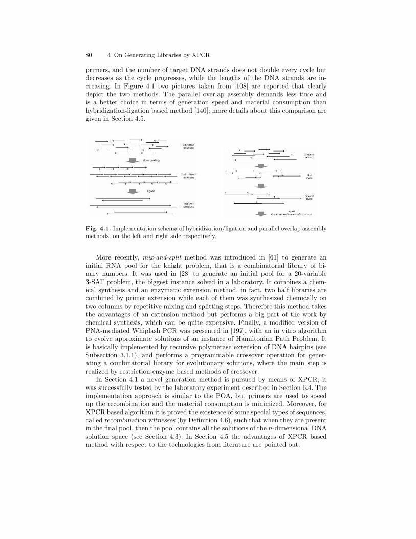
80 4 On Generating Libraries by XPCR
primers, and the number of target DNA strands does not double every cycle butdecreases as the cycle progresses, while the lengths of the DNA strands are in-creasing. In Figure 4.1 two pictures taken from [108] are reported that clearlydepict the two methods. The parallel overlap assembly demands less time andis a better choice in terms of generation speed and material consumption thanhybridization-ligation based method [140]; more details about this comparison aregiven in Section 4.5.
Fig. 4.1. Implementation schema of hybridization/ligation and parallel overlap assemblymethods, on the left and right side respectively.
More recently, mix-and-split method was introduced in [61] to generate aninitial RNA pool for the knight problem, that is a combinatorial library of bi-nary numbers. It was used in [28] to generate an initial pool for a 20-variable3-SAT problem, the biggest instance solved in a laboratory. It combines a chem-ical synthesis and an enzymatic extension method, in fact, two half libraries arecombined by primer extension while each of them was synthesized chemically ontwo columns by repetitive mixing and splitting steps. Therefore this method takesthe advantages of an extension method but performs a big part of the work bychemical synthesis, which can be quite expensive. Finally, a modified version ofPNA-mediated Whiplash PCR was presented in [197], with an in vitro algorithmto evolve approximate solutions of an instance of Hamiltonian Path Problem. Itis basically implemented by recursive polymerase extension of DNA hairpins (seeSubsection 3.1.1), and performs a programmable crossover operation for gener-ating a combinatorial library for evolutionary solutions, where the main step isrealized by restriction-enzyme based methods of crossover.
In Section 4.1 a novel generation method is pursued by means of XPCR; itwas successfully tested by the laboratory experiment described in Section 6.4. Theimplementation approach is similar to the POA, but primers are used to speedup the recombination and the material consumption is minimized. Moreover, forXPCR based algorithm it is proved the existence of some special types of sequences,called recombination witnesses (by Definition 4.6), such that when they are presentin the final pool, then the pool contains all the solutions of the n-dimensional DNAsolution space (see Section 4.3). In Section 4.5 the advantages of XPCR basedmethod with respect to the technologies from literature are pointed out.
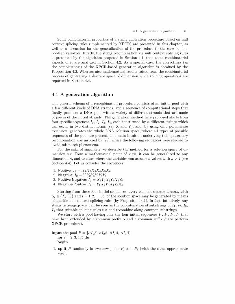
4.1 A generation algorithm 81
Some combinatorial properties of a string generation procedure based on nullcontext splicing rules (implemented by XPCR) are presented in this chapter, aswell as a discussion for the generalization of the procedure to the case of non-boolean variables. Firstly, the string recombination via null context splicing rulesis presented by the algorithm proposed in Section 4.1, then some combinatorialaspects of it are analyzed in Section 4.2. As a special case, the correctness (asthe completeness) of the XPCR-based generation algorithm is obtained by theProposition 4.2. Whereas nice mathematical results raised from the combinatorialprocess of generating a discrete space of dimension n via splicing operations arereported in Section 4.4.
4.1 A generation algorithm
The general schema of a recombination procedure consists of an initial pool witha few different kinds of DNA strands, and a sequence of computational steps thatfinally produces a DNA pool with a variety of different strands that are madeof pieces of the initial strands. The generation method here proposed starts fromfour specific sequences I1, I2, I3, I4, each constituted by n different strings whichcan occur in two distinct forms (say X and Y), and, by using only polymeraseextension, generates the whole DNA solution space, where all types of possiblesequences of the pool are present. The main intuition underlying this quaternaryrecombination was inspired by [28], where the following sequences were studied toavoid mismatch phenomena.
For the sake of simplicity we describe the method for a solution space of di-mension six. From a mathematical point of view, it can be generalized to anydimension n, and to cases where the variables can assume k values with k > 2 (seeSection 4.4). Let us consider the sequences:
1. Positive: I1 = X1X2X3X4X5X6
2. Negative: I2 = Y1Y2Y3Y4Y5Y6
3. Positive-Negative: I3 = X1Y2X3Y4X5Y6
4. Negative-Positive: I4 = Y1X2Y3X4Y5X6
Starting from these four initial sequences, every element α1α2α3α4α5α6, withαi ∈ {Xi, Yi} and i = 1, 2, . . . , 6, of the solution space may be generated by meansof specific null context splicing rules (by Proposition 4.1). In fact, intuitively, anystring α1α2α3α4α5α6 can be seen as the concatenation of substrings of I1, I2, I3,I4 that suitable splicing rules cut and recombine along common substrings.
We start with a pool having only the four initial sequences I1, I2, I3, I4 thathave been extended by a common prefix α and a common suffix β (to performXPCR procedure).
input the pool P = {αI1β, αI2β, αI3β, αI4β}for i = 2, 3, 4, 5 dobegin
1. split P randomly in two new pools P1 and P2 (with the same approximatesize);
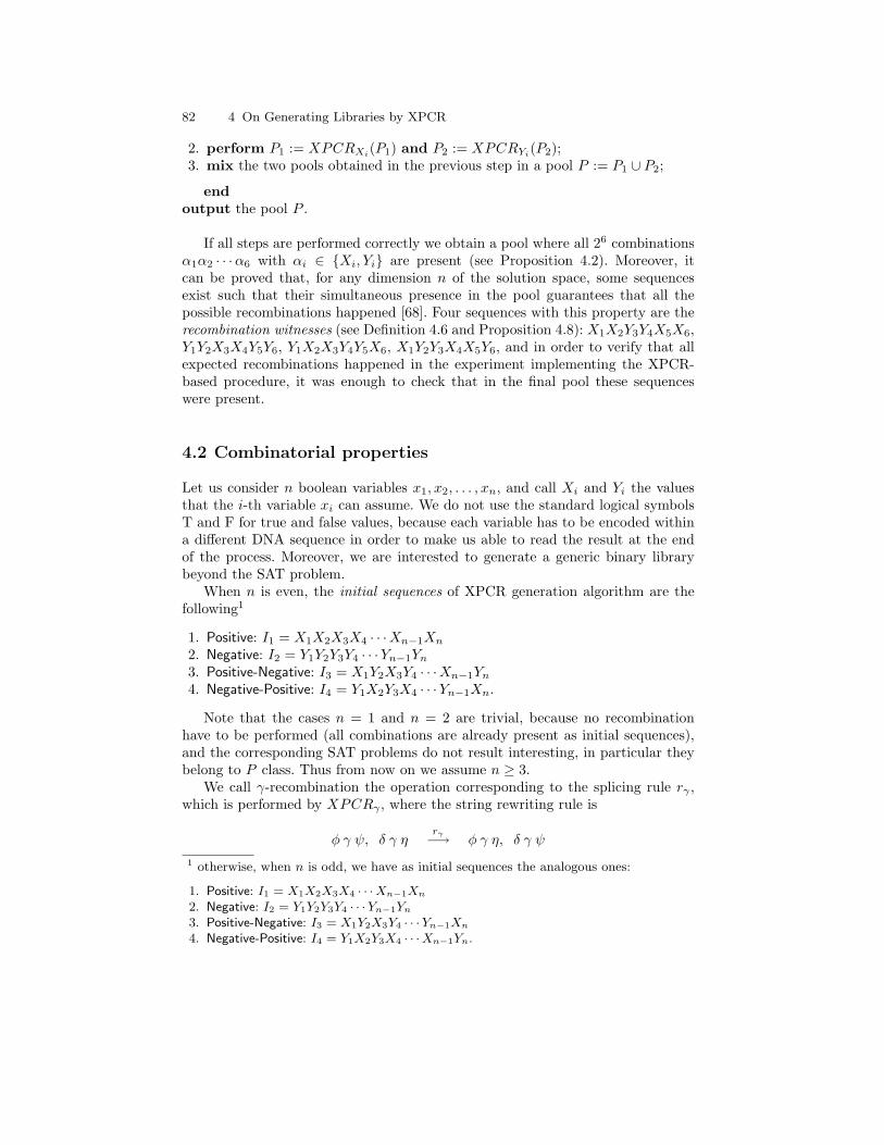
82 4 On Generating Libraries by XPCR
2. perform P1 := XPCRXi(P1) and P2 := XPCRYi
(P2);3. mix the two pools obtained in the previous step in a pool P := P1 ∪ P2;
endoutput the pool P .
If all steps are performed correctly we obtain a pool where all 26 combinationsα1α2 · · ·α6 with αi ∈ {Xi, Yi} are present (see Proposition 4.2). Moreover, itcan be proved that, for any dimension n of the solution space, some sequencesexist such that their simultaneous presence in the pool guarantees that all thepossible recombinations happened [68]. Four sequences with this property are therecombination witnesses (see Definition 4.6 and Proposition 4.8): X1X2Y3Y4X5X6,Y1Y2X3X4Y5Y6, Y1X2X3Y4Y5X6, X1Y2Y3X4X5Y6, and in order to verify that allexpected recombinations happened in the experiment implementing the XPCR-based procedure, it was enough to check that in the final pool these sequenceswere present.
4.2 Combinatorial properties
Let us consider n boolean variables x1, x2, . . . , xn, and call Xi and Yi the valuesthat the i-th variable xi can assume. We do not use the standard logical symbolsT and F for true and false values, because each variable has to be encoded withina different DNA sequence in order to make us able to read the result at the endof the process. Moreover, we are interested to generate a generic binary librarybeyond the SAT problem.
When n is even, the initial sequences of XPCR generation algorithm are thefollowing1
1. Positive: I1 = X1X2X3X4 · · ·Xn−1Xn
2. Negative: I2 = Y1Y2Y3Y4 · · ·Yn−1Yn
3. Positive-Negative: I3 = X1Y2X3Y4 · · ·Xn−1Yn
4. Negative-Positive: I4 = Y1X2Y3X4 · · ·Yn−1Xn.
Note that the cases n = 1 and n = 2 are trivial, because no recombinationhave to be performed (all combinations are already present as initial sequences),and the corresponding SAT problems do not result interesting, in particular theybelong to P class. Thus from now on we assume n ≥ 3.
We call γ-recombination the operation corresponding to the splicing rule rγ ,which is performed by XPCRγ , where the string rewriting rule is
φ γ ψ, δ γ ηrγ−→ φ γ η, δ γ ψ
1 otherwise, when n is odd, we have as initial sequences the analogous ones:
1. Positive: I1 = X1X2X3X4 · · ·Xn−1Xn
2. Negative: I2 = Y1Y2Y3Y4 · · ·Yn−1Yn
3. Positive-Negative: I3 = X1Y2X3Y4 · · ·Yn−1Xn
4. Negative-Positive: I4 = Y1X2Y3X4 · · ·Xn−1Yn.
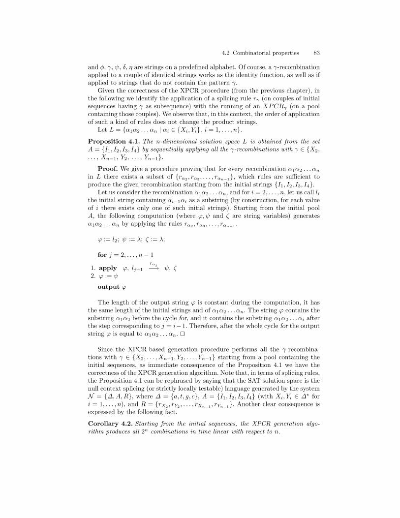
4.2 Combinatorial properties 83
and φ, γ, ψ, δ, η are strings on a predefined alphabet. Of course, a γ-recombinationapplied to a couple of identical strings works as the identity function, as well as ifapplied to strings that do not contain the pattern γ.
Given the correctness of the XPCR procedure (from the previous chapter), inthe following we identify the application of a splicing rule rγ (on couples of initialsequences having γ as subsequence) with the running of an XPCRγ (on a poolcontaining those couples). We observe that, in this context, the order of applicationof such a kind of rules does not change the product strings.
Let L = {α1α2 . . . αn | αi ∈ {Xi, Yi}, i = 1, . . . , n}.
Proposition 4.1. The n-dimensional solution space L is obtained from the setA = {I1, I2, I3, I4} by sequentially applying all the γ-recombinations with γ ∈ {X2,. . . , Xn−1, Y2, . . . , Yn−1}.
Proof. We give a procedure proving that for every recombination α1α2 . . . αn
in L there exists a subset of {rα2 , rα3 , . . . , rαn−1}, which rules are sufficient toproduce the given recombination starting from the initial strings {I1, I2, I3, I4}.
Let us consider the recombination α1α2 . . . αn, and for i = 2, . . . , n, let us call lithe initial string containing αi−1αi as a substring (by construction, for each valueof i there exists only one of such initial strings). Starting from the initial poolA, the following computation (where ϕ,ψ and ζ are string variables) generatesα1α2 . . . αn by applying the rules rα2 , rα3 , . . . , rαn−1 .
ϕ := l2; ψ := λ; ζ := λ;
for j = 2, . . . , n− 1
1. apply ϕ, lj+1
rαj−→ ψ, ζ2. ϕ := ψ
output ϕ
The length of the output string ϕ is constant during the computation, it hasthe same length of the initial strings and of α1α2 . . . αn. The string ϕ contains thesubstring α1α2 before the cycle for, and it contains the substring α1α2 . . . αi afterthe step corresponding to j = i−1. Therefore, after the whole cycle for the outputstring ϕ is equal to α1α2 . . . αn. ut
Since the XPCR-based generation procedure performs all the γ-recombina-tions with γ ∈ {X2, . . . , Xn−1, Y2, . . . , Yn−1} starting from a pool containing theinitial sequences, as immediate consequence of the Proposition 4.1 we have thecorrectness of the XPCR generation algorithm. Note that, in terms of splicing rules,the Proposition 4.1 can be rephrased by saying that the SAT solution space is thenull context splicing (or strictly locally testable) language generated by the systemN = {∆,A,R}, where ∆ = {a, t, g, c}, A = {I1, I2, I3, I4} (with Xi, Yi ∈ ∆? fori = 1, . . . , n), and R = {rX2 , rY2 , . . . , rXn−1 , rYn−1}. Another clear consequence isexpressed by the following fact.
Corollary 4.2. Starting from the initial sequences, the XPCR generation algo-rithm produces all 2n combinations in time linear with respect to n.

84 4 On Generating Libraries by XPCR
Proof. By Proposition 4.1 we claim that if all the possible γ-recombinationshave happened starting from the initial strands (that is XPCR generation al-gorithm was entirely executed), then all the 2n combinations α1α2 . . . αn withαi ∈ {Xi, Yi} have been produced in the final pool.
XPCR generation algorithm by definition performs 2(n− 2) steps by applyingall the splicing rules rγ with γ = X2, . . . , Xn−1, Y2, . . . , Yn−1, that is, it has a linearcomplexity with respect the size of the problem n. ut
Conversely, for any value of n, the presence of only two specific sequences (re-combination witnesses) in the final pool guarantees that all the γ-recombinations,with γ = X2, . . . , Xn−1, Y2, . . . , Yn−1, have been performed starting from a poolcontaining the four initial sequences. Consequently, by Proposition 4.1, such apresence guarantees that any combination in L is present in the final pool, too.
The existence of recombination witnesses is interesting from both theoreticaland experimental points of view, let us explain the theory behind it.
Definition 4.3. Let αi ∈ {Xi, Yi}. We say that αi is positive if it is equal to Xi
and is negative if it is equal to Yi.
We note that, for i = 2, . . . , n − 1 and for any sign (positive or negative) ofξi ∈ {Xi, Yi}, a sequence αi−1 ξi αi+1 has exactly two consecutive variables witha same sign in only two cases:
1. ξi has sign equal to the sign of αi−1 and different from the sign of αi+1 (thatis, αi−1 ξi αi+1 is Xi−1XiYi+1 if ξi = Xi and is Yi−1YiXi+1 if ξi = Yi),
2. ξi has sign equal to the sign of αi+1 and different from the sign of αi−1 (thatis, αi−1 ξi αi+1 is Yi−1XiXi+1 if ξi = Xi and is Xi−1YiYi+1 if ξi = Yi).
Definition 4.4. We call ξi-trio factor any substring αi−1ξiαi+1 where there areexactly two consecutive variables with a same sign, and ξi-target a string whichincludes a ξi-trio factor.
If i 6= j then a ξi-target can be a ξj-target, and in general, for i = 2, . . . , n− 1,the intersections between sets of ξi-target strings are nonempty. While a Xi-targetsequence cannot be a Yi-target sequence, for any value of i, because each string ofthe pool contains either Xi or Yi.
If we assume that the XPCR based generation algorithm has run on a poolcontaining the four initial sequences, then the following result holds.
Lemma 4.5. For any i = 2, . . . , n− 1, the rule rξi has been applied iff in the poolthere is a ξi-target string.
Proof. Let us consider a fixed value of i.
Only if) We show that the application of the rule rξion a (uniquely determined)
couple of initial strings generates (only) strings including a ξi-trio factor.If i is even, then the application of rξi
can be either (case ξi = Xi)
I1, I4rXi−→ φ Xi−1XiYi+1 η, δ Yi−1XiXi+1 ψ
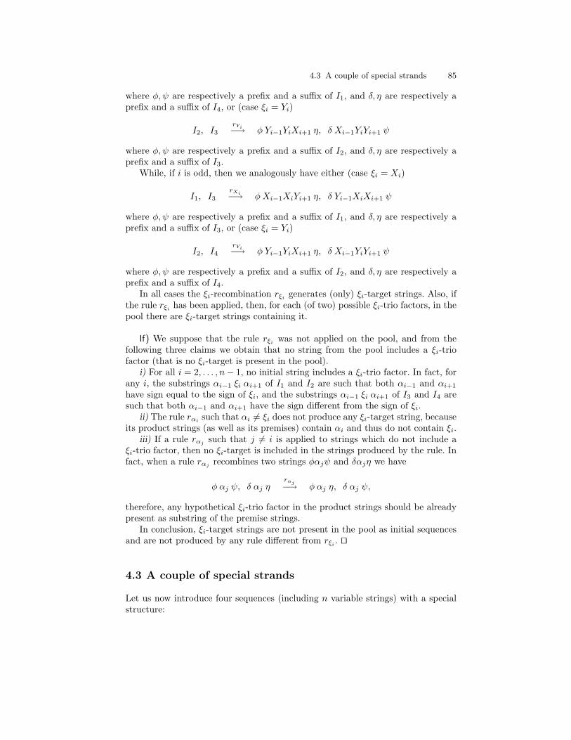
4.3 A couple of special strands 85
where φ, ψ are respectively a prefix and a suffix of I1, and δ, η are respectively aprefix and a suffix of I4, or (case ξi = Yi)
I2, I3rYi−→ φ Yi−1YiXi+1 η, δ Xi−1YiYi+1 ψ
where φ, ψ are respectively a prefix and a suffix of I2, and δ, η are respectively aprefix and a suffix of I3.
While, if i is odd, then we analogously have either (case ξi = Xi)
I1, I3rXi−→ φ Xi−1XiYi+1 η, δ Yi−1XiXi+1 ψ
where φ, ψ are respectively a prefix and a suffix of I1, and δ, η are respectively aprefix and a suffix of I3, or (case ξi = Yi)
I2, I4rYi−→ φ Yi−1YiXi+1 η, δ Xi−1YiYi+1 ψ
where φ, ψ are respectively a prefix and a suffix of I2, and δ, η are respectively aprefix and a suffix of I4.
In all cases the ξi-recombination rξi generates (only) ξi-target strings. Also, ifthe rule rξi
has been applied, then, for each (of two) possible ξi-trio factors, in thepool there are ξi-target strings containing it.
If) We suppose that the rule rξi was not applied on the pool, and from thefollowing three claims we obtain that no string from the pool includes a ξi-triofactor (that is no ξi-target is present in the pool).
i) For all i = 2, . . . , n− 1, no initial string includes a ξi-trio factor. In fact, forany i, the substrings αi−1 ξi αi+1 of I1 and I2 are such that both αi−1 and αi+1
have sign equal to the sign of ξi, and the substrings αi−1 ξi αi+1 of I3 and I4 aresuch that both αi−1 and αi+1 have the sign different from the sign of ξi.
ii) The rule rαi such that αi 6= ξi does not produce any ξi-target string, becauseits product strings (as well as its premises) contain αi and thus do not contain ξi.
iii) If a rule rαjsuch that j 6= i is applied to strings which do not include a
ξi-trio factor, then no ξi-target is included in the strings produced by the rule. Infact, when a rule rαj
recombines two strings φαjψ and δαjη we have
φ αj ψ, δ αj ηrαj−→ φ αj η, δ αj ψ,
therefore, any hypothetical ξi-trio factor in the product strings should be alreadypresent as substring of the premise strings.
In conclusion, ξi-target strings are not present in the pool as initial sequencesand are not produced by any rule different from rξi . ut
4.3 A couple of special strands
Let us now introduce four sequences (including n variable strings) with a specialstructure:
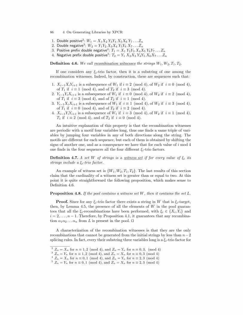
86 4 On Generating Libraries by XPCR
1. Double positive2: W1 = X1X2 Y3Y4 X5X6 Y7 . . . Zn
2. Double negative3: W2 = Y1Y2 X3X4 Y5Y6 X7 . . . Zn
3. Positive prefix double negative4: T1 = X1 Y2Y3 X4X5 Y6Y7 . . . Zn
4. Negative prefix double positive5: T2 = Y1 X2X3 Y4Y5 X6X7 . . . Zn
Definition 4.6. We call recombination witnesses the strings W1,W2, T1, T2.
If one considers any ξi-trio factor, then it is a substring of one among therecombination witnesses. Indeed, by construction, these are sequences such that:
1. Xi−1XiYi+1 is a subsequence of W1 if i ≡ 2 (mod 4), of W2 if i ≡ 0 (mod 4),of T1 if i ≡ 1 (mod 4), and of T2 if i ≡ 3 (mod 4).
2. Yi−1YiXi+1 is a subsequence of W1 if i ≡ 0 (mod 4), of W2 if i ≡ 2 (mod 4),of T1 if i ≡ 3 (mod 4), and of T2 if i ≡ 1 (mod 4).
3. Yi−1XiXi+1 is a subsequence of W1 if i ≡ 1 (mod 4), of W2 if i ≡ 3 (mod 4),of T1 if i ≡ 0 (mod 4), and of T2 if i ≡ 2 (mod 4).
4. Xi−1YiYi+1 is a subsequence of W1 if i ≡ 3 (mod 4), of W2 if i ≡ 1 (mod 4),T1 if i ≡ 2 (mod 4), and of T2 if i ≡ 0 (mod 4).
An intuitive explanation of this property is that the recombination witnessesare periodic with a motif four variables long, thus one finds a same triple of vari-ables by jumping four variables in any of both directions along the string. Themotifs are different for each sequence, but each of them is obtained by shifting thesigns of another one, and as a consequence we have that for each value of i mod 4one finds in the four sequences all the four different ξi-trio factors.
Definition 4.7. A set W of strings is a witness set if for every value of ξi itsstrings include a ξi-trio factor.
An example of witness set is {W1,W2, T1, T2}. The last results of this sectionclaim that the cardinality of a witness set is greater than or equal to two. At thispoint it is quite straightforward the following proposition, which makes sense toDefinition 4.6.
Proposition 4.8. If the pool contains a witness set W , then it contains the set L.
Proof. Since for any ξi-trio factor there exists a string in W that is ξi-target,then, by Lemma 4.5, the presence of all the elements of W in the pool guaran-tees that all the ξi-recombinations have been performed, with ξi ∈ {Xi, Yi} andi = 2, . . . , n− 1. Therefore, by Proposition 4.1, it guarantees that any recombina-tion α1α2 . . . αn from L is present in the pool. ut
A characterization of the recombination witnesses is that they are the onlyrecombinations that cannot be generated from the initial strings by less than n−2splicing rules. In fact, every their substring three variables long is a ξi-trio factor for
2 Zn = Xn for n ≡ 1, 2 (mod 4), and Zn = Yn for n ≡ 0, 3, (mod 4)3 Zn = Yn for n ≡ 1, 2 (mod 4), and Zn = Xn for n ≡ 0, 3 (mod 4)4 Zn = Xn for n ≡ 0, 1 (mod 4), and Zn = Yn for n ≡ 2, 3 (mod 4)5 Zn = Yn for n ≡ 0, 1 (mod 4), and Zn = Xn for n ≡ 2, 3 (mod 4)
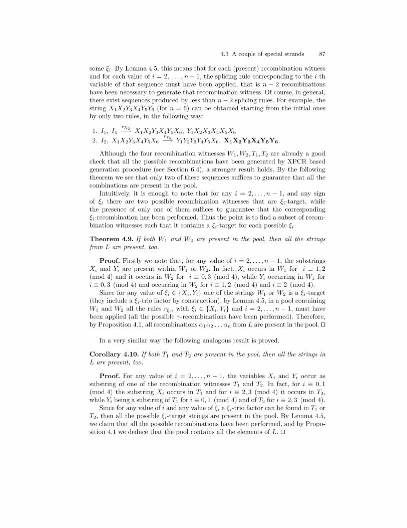
4.3 A couple of special strands 87
some ξi. By Lemma 4.5, this means that for each (present) recombination witnessand for each value of i = 2, . . . , n− 1, the splicing rule corresponding to the i-thvariable of that sequence must have been applied, that is n − 2 recombinationshave been necessary to generate that recombination witness. Of course, in general,there exist sequences produced by less than n− 2 splicing rules. For example, thestring X1X2Y3X4Y5Y6 (for n = 6) can be obtained starting from the initial onesby only two rules, in the following way:
1. I1, I4rX2−→ X1X2Y3X4Y5X6, Y1X2X3X4X5X6
2. I2, X1X2Y3X4Y5X6
rY5−→ Y1Y2Y3Y4Y5X6, X1X2Y3X4Y5Y6.
Although the four recombination witnesses W1,W2, T1, T2 are already a goodcheck that all the possible recombinations have been generated by XPCR basedgeneration procedure (see Section 6.4), a stronger result holds. By the followingtheorem we see that only two of these sequences suffices to guarantee that all thecombinations are present in the pool.
Intuitively, it is enough to note that for any i = 2, . . . , n − 1, and any signof ξi there are two possible recombination witnesses that are ξi-target, whilethe presence of only one of them suffices to guarantee that the correspondingξi-recombination has been performed. Thus the point is to find a subset of recom-bination witnesses such that it contains a ξi-target for each possible ξi.
Theorem 4.9. If both W1 and W2 are present in the pool, then all the stringsfrom L are present, too.
Proof. Firstly we note that, for any value of i = 2, . . . , n − 1, the substringsXi and Yi are present within W1 or W2. In fact, Xi occurs in W1 for i ≡ 1, 2(mod 4) and it occurs in W2 for i ≡ 0, 3 (mod 4), while Yi occurring in W1 fori ≡ 0, 3 (mod 4) and occurring in W2 for i ≡ 1, 2 (mod 4) and i ≡ 2 (mod 4).
Since for any value of ξi ∈ {Xi, Yi} one of the strings W1 or W2 is a ξi-target(they include a ξi-trio factor by construction), by Lemma 4.5, in a pool containingW1 and W2 all the rules rξi
, with ξi ∈ {Xi, Yi} and i = 2, . . . , n − 1, must havebeen applied (all the possible γ-recombinations have been performed). Therefore,by Proposition 4.1, all recombinations α1α2 . . . αn from L are present in the pool. ut
In a very similar way the following analogous result is proved.
Corollary 4.10. If both T1 and T2 are present in the pool, then all the strings inL are present, too.
Proof. For any value of i = 2, . . . , n − 1, the variables Xi and Yi occur assubstring of one of the recombination witnesses T1 and T2. In fact, for i ≡ 0, 1(mod 4) the substring Xi occurs in T1 and for i ≡ 2, 3 (mod 4) it occurs in T2,while Yi being a substring of T1 for i ≡ 0, 1 (mod 4) and of T2 for i ≡ 2, 3 (mod 4).
Since for any value of i and any value of ξi a ξi-trio factor can be found in T1 orT2, then all the possible ξi-target strings are present in the pool. By Lemma 4.5,we claim that all the possible recombinations have been performed, and by Propo-sition 4.1 we deduce that the pool contains all the elements of L. ut

88 4 On Generating Libraries by XPCR
The presence of only a couple of recombinations witnesses suffices to guaranteethat the pool contains all the possible recombinations, but the couple has to be{W1,W2} or {T1, T2}, it cannot contain one between W1 and W2 and the other onebetween T1 and T2. In fact, T1 and W1 can be present in the pool also when, forexample, rX3 , rY5 , rX7 were not applied (in fact both of them do not contain anyX3-trio factor, Y5-trio factor, X7-trio factor), T1 and W2 can be similarly presentalso if rX2 and rY4 were not performed, and the presence of T2 and W1 does notshow anything about the application of rY2 , rX4 or rY6 . Finally, T2 and W2 arepresent also if, for example, only the recombination rX3 was executed with respectto the third variable (i.e., if rY3 was not executed).
An obvious characterization of a ‘sound’ couple of recombination witnesses,that can be {W1,W2} or {T1, T2}, is that the set of splicing rules necessary toproduce its strings cannot be smaller than the set of all the recombination rulesrγ with γ ∈ {X2, . . . , Xn−1, Y1, . . . , Yn−1}. In fact, for each variable αi, one stringof such a witness set must contain Xi and the other one must contain Yi.
Therefore, two is the minimum number of recombination witnesses testing thepresence of the whole solution space L in the pool.
Corollary 4.11. The presence of one recombination witness in the pool does notguarantee that all the recombinations belonging to L are present.
Proof. It is enough to note that in the pool the string W1 can be present evenif all the rules rXi
and rYjwith i ≡ 0, 3 (mod 4) and j ≡ 1, 2 (mod 4) have been
not applied, the string W2 can be present even if all the rules rXiand rYj
withi ≡ 1, 2 (mod 4) and j ≡ 0, 3 (mod 4) have been not applied, the string T1 can bepresent even if all the rules rXi and rYj with i ≡ 2, 3 (mod 4) and j ≡ 0, 1 (mod 4)have been not applied, and the string T4 can be present even if all the rules rXi
and rYjwith i ≡ 0, 1 (mod 4) and j ≡ 2, 3 (mod 4) have been not applied. ut
For the scaling up purpose of DNA computing and for the sake of mathematicalgenerality, we note that all the results here proposed are valid for any value of n.In general, if k (greater than or equal to two) is the number of values that eachvariable can assume, the minimum number of recombination witnesses testingthe presence of the corresponding solution space, as well as the number of initialsequences, depends only on the value of k, as k and k2 respectively.
4.4 Generalized generation algorithm
If the k different values that the i-th variable can assume are denoted by theelements of {Z(1)
i , . . . , Z(k)i }, for i = 1, . . . , n, then we define the following strings6.
• W1 = Z(1)1 Z
(1)2 Z
(2)3 Z
(2)4 Z
(1)5 Z
(1)6 Z
(2)7 Z
(2)8 Z
(1)9 · · ·Z
(p1)n
• W2 = Z(2)1 Z
(2)2 Z
(3)3 Z
(3)4 Z
(2)5 Z
(2)6 Z
(3)7 Z
(3)8 Z
(2)9 · · ·Z
(p2)n
6 If n ≡ 1, 2 (mod 4) then pm = m form = 1, . . . , k. If n ≡ 0, 4 (mod 4) then pm = m+1for m = 1, . . . , k − 1, and pk = 1.

4.4 Generalized generation algorithm 89
• for j = 3, . . . , k − 1Wj = Z
(j)1 Z
(j)2 Z
(j+1)3 Z
(j+1)4 Z
(j)5 Z
(j)6 Z
(j+1)7 Z
(j+1)8 Z
(j)9 · · ·Z
(pj)n
• Wk = Z(k)1 Z
(k)2 Z
(1)3 Z
(1)4 Z
(k)5 Z
(k)6 Z
(1)7 Z
(1)8 Z
(k)9 · · ·Z(pk)
n
Definition 4.12. We call k-recombination witnesses the strings W1,W2, . . . ,Wk.
The analogue of Theorem 4.9 holds also in this general case. Theorem 4.17is proved after the introduction of Lemma 4.16, that is a generalized version ofLemma 4.5. Let Gk = {α1α2 . . . αn | αi ∈ {Z(1)
i , . . . , Z(k)i }, i = 1, . . . , n} for k ≥ 2.
It is a generalization of a binary solution space, in fact G2 = L.All the results of the previous section can be generalized to the general case
of k ∈ N. In fact, the n-dimensional k-solution space Gk formed by all thekn recombinations of n variables assuming k different values can be generatedby applying k(n − 2) splicing rules. From an experimental viewpoint, a XPCR-based generation algorithm performing all the XPCRγ with γ ∈ {Z(1)
2 , . . . , Z(k)2 ,
Z(1)3 , . . . , Z
(k)3 ,. . . , Z(1)
n−1, . . . , Z(k)n−1} on a pool containing the following (initial)
strings produces the solution space Gk in linear time.
The initial sequences I1, . . . , Ik2 are defined by the expression, for i, j = 1, . . . , kand n even7
I(i−1)k+j = Z(i)1 Z
(j)2 Z
(i)3 Z
(j)4 · · ·Z
(i)n−1Z
(j)n
For an example, let us assume n even and k = 3, and suppose that the i-thvariable takes values in {ai, bi, ci}, then the initial sequences are
• (for i = 1 and j = 1, 2, 3)
I1 = a1a2 . . . an, I2 = a1b2a3b4 . . . bn, I3 = a1c2a3c4 . . . cn,
• (for i = 2 and j = 1, 2, 3)
I4 = b1a2b3a4 . . . an, I5 = b1b2 . . . bn, I6 = b1c2b3c4 . . . cn,
• (for i = 3 and j = 1, 2, 3)
I7 = c1a2c3a4 . . . an, I8 = c1b2c3b4 . . . bn, I9 = c1c2 . . . cn.
Note that for any initial sequence I(i−1)k+j , i is ‘the sign’ of the variables withindex odd and j is ‘the sign’ of the variables with index even. The generalizedversion of the XPCR based generation algorithm follows.
input the pool P = {αI1β, αI2β, . . . , αIk2β}
for i = 2, 3, 4, . . . , n− 1 dobegin
1. split P randomly in k new pools P1, P2, . . . , Pk (with the same approximatesize);
7 otherwise, when n is odd, we have the analogous ones, for i, j ∈ {1, 2, . . . , k}I(i−1)k+j = Z
(i)1 Z
(j)2 Z
(i)3 Z
(j)4 · · ·Z(j)
n−1Z(i)n

90 4 On Generating Libraries by XPCR
2. perform Pj := XPCRZ
(j)i
(Pj) for j = 1, . . . , k;3. mix the k pools obtained in the previous step in a pool P := P1∪P2∪· · ·∪Pk;
end
output the pool P .
Proposition 4.13. The n-dimensional k-solution space Gk is obtained from theset A = {I1, I2, . . . , Ik2} of initial sequences by applying all the γ-recombinationsrγ with γ ∈ {Z(1)
2 , . . . , Z(k)2 , Z
(1)3 , . . . , Z
(k)3 ,. . . , Z(1)
n−1, . . . , Z(k)n−1}.
Proof. We give a procedure proving that every recombination α1α2 . . . αn inGk is generated by applying the corresponding splicing rules {rα2 , rα3 , . . . , rαn−1}to couples of initial sequences from {I1, I2, . . . , Ik2}.
Let us consider the recombination α1α2 . . . αn from Gk, and for i = 2, . . . , n,let us call li the initial sequence containing αi−1αi as substring. By construction,for each value of i there exists only one of such an initial string. In fact, if αi isequal to Za
i and αi−1 is equal to Z(b)i−1, then αi−1αi is a subsequence of I(b−1)k+a
if i ≡ 0 (mod 2), and it is a subsequence of I(a−1)k+b if i ≡ 1 (mod 2).The following computation (where ϕ, ψ and ζ are string variables) generates
α1α2 . . . αn by applying the recombinations rα2 , rα3 , . . . , rαn−1 on some initial se-quences from A.
ϕ := l2; ψ := λ; ζ := λ;
for j = 2, . . . , n− 1
1. apply ϕ, lj+1
rαj−→ ψ, ζ2. ϕ := ψ
output ϕ
The length of the output string ϕ is constant during the computation, it hasthe same length of the initial strings and of α1α2 . . . αn. The string ϕ contains thesubstring α1α2 before the cycle for, and it contains the substring α1α2 . . . αi afterthe step corresponding to j = i−1. Therefore, after the whole cycle for the outputstring ϕ is equal to α1α2 . . . αn. ut
Note that any recombination is generated by (at most) n − 2 splicing rules,regardless the number of values that each variable can assume. The generalizationof Lemma 4.5 follows.
Definition 4.14. Let α(u)i , ξ
(v)i ∈ {Z(1)
i , . . . , Z(k)i }. We say that α(u)
i and ξ(v)j
have the same sign if u = v, otherwise we say they have a different sign.
Definition 4.15. We call ξ(h)i -trio factor any substring α(u)
i−1 ξ(h)i α
(v)i+1 where there
are exactly two consecutive variables with a same sign, and ξ(h)i -target a string
which includes a ξ(h)i -trio factor.

4.4 Generalized generation algorithm 91
Let us assume that the XPCR based generation algorithm has run on a poolcontaining the k initial sequences, then
Lemma 4.16. Any rule rξ(h)i
has been applied iff in the pool there is a ξ(h)i -target
string.
Proof. Let us consider a fixed value of i.
Only if) We show that the application of the rule rξ(h)i
on a couple of initial
sequences generates ξ(h)i -target strings. Such a couple is not uniquely determined,
in fact for each value of ξ(h)i there are k different initial sequences that contain
ξ(h)i as substring.
We can apply the rule rξ(h)i
on initial sequences having α(u)i−1ξ
(h)i α
(u)i+1 as sub-
sequence, where either u = h or u 6= h. Since there is only the initial sequenceI(h−1)k+h having (all) adjacent variables with the same sign h, then we distinguishonly two kinds of couples (of initial sequences) by means of the sign of the variablesadjacent to ξ(h)
i : or the couple contains the sequence I(h−1)k+h or it does not.Let us assume that i is even. If the couple of premises contains the sequence
I(h−1)k+h, then the application of rξ(h)i
works as in the following:
I(h−1)k+h, I(u−1)k+h
rξ(h)i−→ φ α
(h)i−1ξ
(h)i α
(u)i+1 η, δ α
(u)i−1ξ
(h)i α
(h)i+1 ψ
where φ, ψ are respectively a prefix and a suffix of I(h−1)k+h, and δ, η are respec-tively a prefix and a suffix of I(u−1)k+h. In the non-trivial case that u 6= h (that isall the times that the rule produces a new recombination), then ξ(h)
i -target stringsare produced.
If the couple of premises does not contain the sequence I(h−1)k+h (case u, v 6=h), then the application of r
ξ(h)i
works as in the following:
I(v−1)k+h, I(u−1)k+h
rξ(h)i−→ φ α
(v)i−1ξ
(h)i α
(u)i+1 η, δ α
(u)i−1ξ
(h)i α
(v)i+1 ψ
where φ, ψ are respectively a prefix and a suffix of I(v−1)k+h, and δ, η are respec-tively a prefix and a suffix of I(u−1)k+h. Note that in this case we do not haveproduction of ξ(h)
i -target strings.Let us assume that i is odd. If I(h−1)k+h is a premise, then the rule r
ξ(h)i
works
as in the following, by producing ξ(h)i -target strings if u 6= h:
I(h−1)k+h, I(u−1)k+h
rξ(h)i−→ φ α
(h)i−1ξ
(h)i α
(u)i+1 η, δ α
(u)i−1ξ
(h)i α
(h)i+1 ψ
where φ, ψ are respectively a prefix and a suffix of I(h−1)k+h, and δ, η are respec-tively a prefix and a suffix of I(u−1)k+h.
Otherwise (case u, v 6= h), we have:
I(h−1)k+v, I(h−1)k+u
rξ(h)i−→ φ α
(v)i−1ξ
(h)i α
(u)i+1 η, δ α
(u)i−1ξ
(h)i α
(v)i+1 ψ

92 4 On Generating Libraries by XPCR
where φ, ψ are respectively a prefix and a suffix of I(h−1)k+v, and δ, η are respec-tively a prefix and a suffix of I(h−1)k+u. Note that in this case we do not haveproduction of any ξ(h)
i -target string.In conclusion, starting from the sequence I(h−1)k+h and any other initial se-
quence containing ξ(h)i , the ξ(h)
i -recombination generates ξ(h)i -target strings. Also,
if the rule rξ(h)i
has been applied, then for each (of the k − 1) possible ξ(h)i -trio
factor, in the pool there are ξ(h)i -target strings containing it.
If) We suppose that the rule rξ(h)i
was not applied on the pool, and from the
following three claims we obtain that no string from the pool includes a ξ(h)i -trio
factor (that is, no ξ(h)i -target is present in the pool).
i) By construction, for every value of i (i = 2, . . . , n − 1) and for every sign h
(h = 1, 2, . . . , k), no initial string includes a ξ(h)i -trio factor. In fact, for any i, and
in each of the k initial sequences containing a ξ(h)i , the substring αi−1 ξ
(h)i αi+1
has both the variables αi−1 and αi+1 having a same sign u (which is equal to hin the sequence I(h−1)k+h and it is different from h in all the other k − 1 initialsequences), thus it is not a ξ(h)
i -trio factor. By definition, we may conclude thatno initial sequence is a ξ(h)
i -target string.ii) The rule r
ξ(v)i
such that v 6= h does not produce any ξ(h)i -target string,
because its product strings (as well as its premises) contain ξ(v)i and thus do not
contain ξ(h)i .
iii) If a rule rαjsuch that j 6= i is applied to strings which do not include a
ξ(h)i -trio factor (for any value of h), then no ξ
(h)i -target strings are produced by
the rule. In fact, when a rule rαjrecombines two strings φαjψ and δαjη we have
φ αj ψ, δ αj ηrαj−→ φ αj η, δ αj ψ
therefore, any hypothetical ξi-trio factor in the product strings should be alreadypresent as substring of the premise strings.
In conclusion, ξ(h)i -target strings are not present in the pool as initial sequences
and are not produced by any rule different from rξ(h)i
. ut
From the above (first part of the) proof we deduce an interesting differencewith respect to the case k = 2. That is, when k > 2 and starting from the initialsequences, the rules rγ generate a set of strings which properly contains the γ-target ones. This observation opens the question whether less than k recombinationwitnesses can be made, with a different structure, in such a way that they testthe presence of the whole solution space. In fact, for k > 2 it seems that alsothe presence of a sequence containing a α
(u)i−1 α
(h)i α
(v)i+1, while u, v, and h being
three different values from the set {1, 2, . . . , k}, could guarantee that r(h)αi has been
applied.However, we conclude this section by proving one of the main results intro-
duced: the presence of k particular sequences in the final pool guarantees that the

4.5 Advantages of XPCR generation 93
whole n-dimensional k-solution space Gk was generated by k(n − 2) null contextsplicing rules starting from the k2 initial sequences.
Theorem 4.17. If the k-recombination witnesses W1,W2, . . . ,Wk are present inthe pool, then all the kn strings of Gk are present, too.
Proof. For any possible value of Z(h)i we may find one k-recombination witness
such that Z(h)i occurs as substring. In particular, it occurs as substring of Wh for
i ≡ 1, 2 (mod 4) and as substring of Wh−1 (or Wk if h = 1) when i ≡ 0, 3 (mod 4).For i = 2, . . . , n − 2, when Z
(h)i is a substring of a k-recombination witness,
the corresponding substring Z(u)i−1Z
(h)i Z
(v)i+1 is a Z(h)
i -trio factor (indeed one valuev or u is equal to h and the other one is different). In other words, for any valueof Z(h)
i there exists a Z(h)i -target string among the k-recombination witnesses.
Therefore, by Lemma 4.16, in a pool containing all the k-recombination wit-nesses all the splicing rules required by the algorithm have been applied. By Propo-sition 4.13, this fact guarantees that the whole k-solution space Gk is present inthe pool. ut
Unless to change the structure of the recombination witnesses, they all needto be present simultaneously in the pool to guarantee the presence of the wholesolution space.
Corollary 4.18. The presence of k-1 k-recombination witnesses in the pool doesnot guarantee that all the recombinations of Gk are present.
Proof. Let j ∈ {1, . . . , k} and i, h ∈ N such that i ≡ 1, 2 (mod 4) andh ≡ 0, 3 (mod 4). By construction, none of the k − 1 recombination witnessesW1, . . . ,Wj−1,Wj+1, . . . ,Wk is a Z
(j)i -target string (and neither a Z
(j+1)h -target
string) because they do not contain Z(j)i (or Z(j+1)
h ). Therefore, by Lemma 4.16,W1, . . . ,Wj−1, Wj+1, . . . ,Wk might be present in a pool where all the splicingrules but r
Z(j)i
and rZ
(j+1)h
were performed, and where, for example, the recombi-
nations of Gk containing Z(j)i are not all present. ut
A future research on the subject of this section could be to study the case (andto find the minimum number of recombination witnesses) where different variablesmay assume a different number of values.
4.5 Advantages of XPCR generation
Apart the mathematical speculations, XPCR-based generation algorithm is a novelmethod to generate DNA libraries, that has several advantages with respect to thetechniques from the DNA computing literature. POA and hybridization/ligationmethods (that are described in the introduction of this chapter) were reviewedin [140] as initial pool generation methods of combinatorial problems. From atheoretical comparison and a few experimental simulations, the conclusion wassuggested that POA is a better choice in terms of generation speed, material
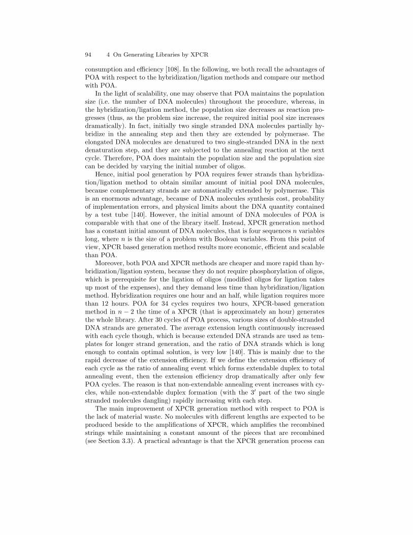
94 4 On Generating Libraries by XPCR
consumption and efficiency [108]. In the following, we both recall the advantages ofPOA with respect to the hybridization/ligation methods and compare our methodwith POA.
In the light of scalability, one may observe that POA maintains the populationsize (i.e. the number of DNA molecules) throughout the procedure, whereas, inthe hybridization/ligation method, the population size decreases as reaction pro-gresses (thus, as the problem size increase, the required initial pool size increasesdramatically). In fact, initially two single stranded DNA molecules partially hy-bridize in the annealing step and then they are extended by polymerase. Theelongated DNA molecules are denatured to two single-stranded DNA in the nextdenaturation step, and they are subjected to the annealing reaction at the nextcycle. Therefore, POA does maintain the population size and the population sizecan be decided by varying the initial number of oligos.
Hence, initial pool generation by POA requires fewer strands than hybridiza-tion/ligation method to obtain similar amount of initial pool DNA molecules,because complementary strands are automatically extended by polymerase. Thisis an enormous advantage, because of DNA molecules synthesis cost, probabilityof implementation errors, and physical limits about the DNA quantity containedby a test tube [140]. However, the initial amount of DNA molecules of POA iscomparable with that one of the library itself. Instead, XPCR generation methodhas a constant initial amount of DNA molecules, that is four sequences n variableslong, where n is the size of a problem with Boolean variables. From this point ofview, XPCR based generation method results more economic, efficient and scalablethan POA.
Moreover, both POA and XPCR methods are cheaper and more rapid than hy-bridization/ligation system, because they do not require phosphorylation of oligos,which is prerequisite for the ligation of oligos (modified oligos for ligation takesup most of the expenses), and they demand less time than hybridization/ligationmethod. Hybridization requires one hour and an half, while ligation requires morethan 12 hours. POA for 34 cycles requires two hours, XPCR-based generationmethod in n − 2 the time of a XPCR (that is approximately an hour) generatesthe whole library. After 30 cycles of POA process, various sizes of double-strandedDNA strands are generated. The average extension length continuously increasedwith each cycle though, which is because extended DNA strands are used as tem-plates for longer strand generation, and the ratio of DNA strands which is longenough to contain optimal solution, is very low [140]. This is mainly due to therapid decrease of the extension efficiency. If we define the extension efficiency ofeach cycle as the ratio of annealing event which forms extendable duplex to totalannealing event, then the extension efficiency drop dramatically after only fewPOA cycles. The reason is that non-extendable annealing event increases with cy-cles, while non-extendable duplex formation (with the 3′ part of the two singlestranded molecules dangling) rapidly increasing with each step.
The main improvement of XPCR generation method with respect to POA isthe lack of material waste. No molecules with different lengths are expected to beproduced beside to the amplifications of XPCR, which amplifies the recombinedstrings while maintaining a constant amount of the pieces that are recombined(see Section 3.3). A practical advantage is that the XPCR generation process can
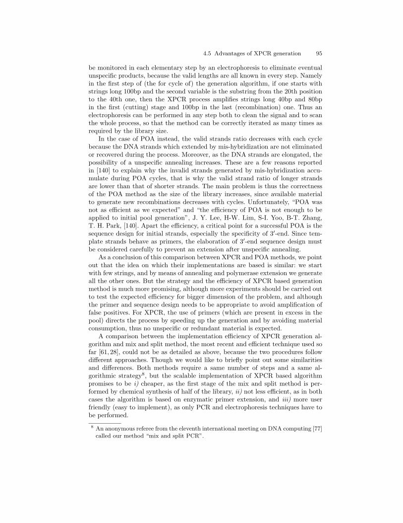
4.5 Advantages of XPCR generation 95
be monitored in each elementary step by an electrophoresis to eliminate eventualunspecific products, because the valid lengths are all known in every step. Namelyin the first step of (the for cycle of) the generation algorithm, if one starts withstrings long 100bp and the second variable is the substring from the 20th positionto the 40th one, then the XPCR process amplifies strings long 40bp and 80bpin the first (cutting) stage and 100bp in the last (recombination) one. Thus anelectrophoresis can be performed in any step both to clean the signal and to scanthe whole process, so that the method can be correctly iterated as many times asrequired by the library size.
In the case of POA instead, the valid strands ratio decreases with each cyclebecause the DNA strands which extended by mis-hybridization are not eliminatedor recovered during the process. Moreover, as the DNA strands are elongated, thepossibility of a unspecific annealing increases. These are a few reasons reportedin [140] to explain why the invalid strands generated by mis-hybridization accu-mulate during POA cycles, that is why the valid strand ratio of longer strandsare lower than that of shorter strands. The main problem is thus the correctnessof the POA method as the size of the library increases, since available materialto generate new recombinations decreases with cycles. Unfortunately, “POA wasnot as efficient as we expected” and “the efficiency of POA is not enough to beapplied to initial pool generation”, J. Y. Lee, H-W. Lim, S-I. Yoo, B-T. Zhang,T. H. Park, [140]. Apart the efficiency, a critical point for a successful POA is thesequence design for initial strands, especially the specificity of 3′-end. Since tem-plate strands behave as primers, the elaboration of 3′-end sequence design mustbe considered carefully to prevent an extension after unspecific annealing.
As a conclusion of this comparison between XPCR and POA methods, we pointout that the idea on which their implementations are based is similar: we startwith few strings, and by means of annealing and polymerase extension we generateall the other ones. But the strategy and the efficiency of XPCR based generationmethod is much more promising, although more experiments should be carried outto test the expected efficiency for bigger dimension of the problem, and althoughthe primer and sequence design needs to be appropriate to avoid amplification offalse positives. For XPCR, the use of primers (which are present in excess in thepool) directs the process by speeding up the generation and by avoiding materialconsumption, thus no unspecific or redundant material is expected.
A comparison between the implementation efficiency of XPCR generation al-gorithm and mix and split method, the most recent and efficient technique used sofar [61, 28], could not be as detailed as above, because the two procedures followdifferent approaches. Though we would like to briefly point out some similaritiesand differences. Both methods require a same number of steps and a same al-gorithmic strategy8, but the scalable implementation of XPCR based algorithmpromises to be i) cheaper, as the first stage of the mix and split method is per-formed by chemical synthesis of half of the library, ii) not less efficient, as in bothcases the algorithm is based on enzymatic primer extension, and iii) more userfriendly (easy to implement), as only PCR and electrophoresis techniques have tobe performed.
8 An anonymous referee from the eleventh international meeting on DNA computing [77]called our method “mix and split PCR”.
96 4 On Generating Libraries by XPCR
On the other hand, the existence of the recombination witnesses (see Sec-tion 4.3) is a check on the experimental iter of our method that represents anactual advantage over all the other existing methods (“The concept of requiringonly two witnesses for the existence of a complete library is a novel and interest-ing one”, anonymous referee8). They provide us with a control of any eventualexperimental error which usually cannot be excluded in any DNA procedure. Theidea here is to give the generation method together with a check (couple of recom-bination witnesses) to control that the method has been implemented correctly,anytime one executes it.
Of course, from a theoretical point of view, we know that the whole libraryis generated because of the correctness of XPCR procedure and XPCR basedgeneration algorithm (i.e., the null context splicing rules required by the algorithmand implemented by XPCR are enough to generate the expected library). But theoperator could possibly wrong or skip some step, or some PCR could not workwell, and unexpected experimental pitfalls could alter the result. If the algorithmwould be automated we would have even less possibilities to check any step withelectrophoresis, and we should trust just the theoretical correctness, as the othermethods usually do. In general, the only way to verify that a library has beenentirely generated is to check each presence experimentally, with an exponentialnumber of steps. Instead, to test the completeness of a library generated by aquaternary recombination of strings via application of null context splicing rules,it is enough to check the presence of two (recombination witnesses) strings. Aswe have seen in the previous sections, this result came up from combinatorialspeculations, while from a biological point of view, we may assume that the XPCRstep, wide experimentally tested, works in parallel and correctly, by involving allthe expected molecules.
However, as a kind of limit of all methods based on PCR, we stress the sensi-tivity of such a reaction: it may be hard to control a process, because unwantedamplification may overcome quite easily, and for any kind of error that should oc-cur, it is amplified with the same rate of the solution. On the other hand, in thosecases where these processes work, they work very well, fast and efficiently. Besides,polymerase chain reaction just resembles in vitro the process of autoduplication ofDNA, thus it is strictly linked to the way cells replicate their genetic code. Also,the aberrant proliferation of a cell very often characterizes its status of tumoredcell, thus in a sense it could be particularly important and interesting to learn tocontrol processes involving DNA replication.
The generation algorithm presented in this chapter, as well as its generalizedform and the combinatorial results, were (respectively) introduced in the papers:
• G. F., V. Manca, C. Giagulli, C. Laudanna, DNA Recombination by XPCR,Revised Selected Paper in A. Carbone, N.A. Pierce Eds: DNA11, June 6-92005, London, Ontario, Canada, LNCS 3892, pp 55-66, 2006.
• G. F., Combinatorial Properties of DNA Libraries Generated via Null ContextSplicing Rules, Discrete Applied Mathematics, submitted.
5
Applications of XPCR
Nature is an infinite sphere of which the center is everywhereand the circumference nowhere.
Blaise Pascal1
The hope of effectively solving NP-problems seems no longer pursued by cur-rent trends of DNA computing. Indeed, after the result proposed in [28], wherea 20 variable instance of SAT was solved in laboratory, researchers have appar-ently abandoned this line of research, and to experimentally progress beyond thisresult seems unlikely. However, the exploration of methods and technologies thatare interesting in itself or useful for something other than solving NP-completeproblems receives wide interest. Although several applications of such proceduresregard genetics and medicine (see Section 5.5), very often NP-complete problemsrepresent a nice way to show that the method or technology works, and severalalgorithms solving combinatorial problems are suggested. This point is faced infurther detail in Chapter 1, along with related references.
In the last two chapters we have presented a method of extraction and one ofgeneration respectively, both implemented on the basis of the XPCR procedure.In this chapter we present more applications of the XPCR technique, such asa theoretical improvement (with a lower complexity) of the XPCR generationmethod in Subsection 5.3.1, and a mutagenesis algorithm (in Section 5.4) that wastested in laboratory by the experiment reported in Section 6.5.
After a presentation of the SAT problem and of its intrinsic complexity inSection 5.1, a polymerase based algorithm for solving an instance of SAT withsignificant size is proposed in Section 5.3. Its extraction step (Subsection 5.3.2)should be implemented by a tricky combination of enzymatic operations, such aspolymerase extension and endonuclease cutting. The aim of Section 5.2 is to brieflyexplain the operations performed by restriction enzymes, since the use of a specificendonuclease is required in the extraction step of the algorithm. Some fascinatingapplications of DNA biotechnologies are outlined in a last section.
1 Pensees, 1670. Quoted in E Maor, To infinity and beyond, Princeton, 1991.

98 5 Applications of XPCR
5.1 The satisfiability problem (SAT)
One of the most intriguing problem to approach by DNA computations is SAT,which has a very simple definition. Given a propositional formula formed by nboolean variables connected by the logical connectives or, and and not, the SATproblem consists in deciding the existence of an assignment of true values to thevariables such that it satisfies the formula. Every instance of a SAT problemcan be written in conjunctive normal form, that is as the conjunction of equationsformed by disjunctions and negations on the variables. A k-SAT (n,m) problem, inparticular, may be seen as a boolean system of m disjunctive equations (clauses)on n variables x1, . . . , xn and their negations ¬x1, . . . ,¬xn (that are all calledliterals li, where i = 1, . . . , n and li ∈ {xi,¬xi}), where each equation contains atmost k literals. If there exists an assignment satisfying the given formula we saythat the formula is satisfiable, and it belongs to the SAT class, otherwise we saythat it is unsatisfiable.
For example, the 3-SAT (2, 2) toy instance (x ∨ y) ∧ (x′ ∨ y′), where x′ is thenegation of x and y′ is the negation of y, was the first to be solved with DNAcomputations, in [143]. There have been huge developments from that experiment(see for example [94,61,154]), and instances of SAT problem up to twenty variableswere solved by encoding data in linear duplex DNA molecules [28]. Recent suc-cessful attempts for solving SAT were done by linear assembly of DNA tiles [237]and by graph self-assembly, where the problem is encoded in duplex and branchedjunction DNA molecules such that the graph can self assemble if and only if thereis a solution to the problem [118].
If k = 1, 2 then a k-SAT problem is solvable with a deterministic Turingmachine in polynomial time, i.e., k-SAT ∈ P . The case k = 1 is trivial, while analgorithm of computational complexity O(n + m) for the 2-SAT (n,m) problemis well known [10]. The case k ≥ 3 is more interesting, because then k-SAT ∈NP . SAT was the first problem shown to be NP-complete (Cook, ’71), and itis nowadays one of most widely studied NP-complete problems. A remarkableconsequence of the theory of NP-completeness is that a large collection of problems(several thousand) from many different fields can be represented as instances of thek-SAT problem. If k ≥ 3 then any instance of k-SAT can be reduced to an instanceof 3-SAT at the cost of linearly increasing the size of the problem, therefore inthe following we will consider only the 3-SAT problem, in order to facilitate theexplanation.
The fastest known heuristic to solve 3-SAT is the Davis-Putnam procedure [90]that is complete and ‘often’ computes in linear time; it performs a backtrack searchthrough the space of possible truth assignments. Although NP-complete problemsare believed to require exponential time to solve in the worst case, the typical-casebehaviour is difficult to characterize. Yet, such typical-case properties are mostrelevant in practical applications.
In terms of what is known theoretically about the probability of satisfiabilityfor random 3-SAT, the threshold conjecture [132] is that there is some specific ratioof clauses to variables above which the probability of satisfiability approaches 1,and below which it approaches 0. The intuitive explanation for this phenomenon isthat at low values of such a ratio we have relatively few clauses and many variables,

5.1 The satisfiability problem (SAT) 99
which means that the formula is relatively easy to satisfy (the problem is under-constrained and a satisfying assignment can be ‘guessed’ quickly). At high values ofthis ratio, the problem is over-constrained and generally no satisfying assignmentexists. The most interesting formulas can be found at the transition from theunder-constrained to the over-constrained area.
In general, NP-complete problems exhibit ‘phase transition’ phenomena, anal-ogous to those in physical systems, while the hardest problems occurring at thephase boundary. Across this phase dramatic changes occur in the computationaldifficulty, and the problems become easier to solve away from the boundary [217]. Amore accurate analysis about the relationship between the computational complex-ity of SAT problems and the phase transition occurring in some physical models asspin glasses [168] was developed in [70], where the application of two methods ofthe statistical mechanics (the annealed estimate and the replica method) to studyk-SAT is discussed.
However, for a 3-SAT (n,m), experimental evidence strongly suggests a thresh-old with m
n ≈ 4.2. In Section 5.3 we consider an algorithm to solve a significantinstance of a random 30-variable 3-SAT problem with 126 clauses, where one hasthe variables x1, x2, . . . , x30, and the clauses C1, C2, . . . , C126, that are the dis-junction of at most three literals.
The crossover point divides the space of satisfiability problems into threeregions: the under-constrained region below the crossover point, the critically-constrained region in the neighborhood of the crossover point, and the over-constrained region above the crossover point. Each of these regions is interest-ing for different reasons. Generally the commercially important satisfiability andconstraint-satisfaction problems are optimization problems: one wants to minimizecosts subject to a given set of constraints. Setting the cost threshold too high re-sults in an under-constrained problem. If instead the cost is set just right oneobtains a critically-constrained problem. Similarly for over-constrained problems.If one has an optimization problem to solve, and one does not have sufficientlypowerful algorithms to solve it in the critically-constrained region (which is usu-ally the case for realistically complex problems), then the only choice is to loosethe cost threshold and to move the problem into the under-constrained region.Thus the under-constrained region is important because in practice it is where op-timization problems are usually ‘solved’. Clearly the critically-constrained regionis important because it is where we must work if we have to solve optimizationproblems exactly. Finally, the over-constrained region is important because show-ing over-constrained problems to be unsolvable corresponds to showing optimalityof solutions to optimization problems.
The location of the crossover point is of both theoretical and practical rele-vance. It is theoretically interesting since, a threshold exists for any value of k, butdetermining the exact location of the threshold remains a difficult open problem,although there has been substantial progress in narrowing the theoretical boundson the transition, and in the case of 3-SAT, the number of constraints required forcrossover appears to be almost (but not exactly) a linear function of the numberof variables in the problem. One reason for the limitations of analytic results isthe complexity of the analysis required. Another is that they are asymptotic withrespect to the number of variables, so they do not necessarily tell us much about

100 5 Applications of XPCR
formulas that have only a modest number of variables (say, up to a few thousand)as encountered in practice. On the other hand, the location of the crossover pointis of practical interest since empirically the hardest problems seem to be foundnear that area, thus it makes sense to test candidate algorithms on these hardproblems. This means that if one knows the location of the crossover point, thenfor random problems (i.e., problems with no structure) the number of clauses canbe used as a predictor of satisfiability.
In order to solve a SAT instance with 30 variables and 126 clauses we aregoing to present a DNA algorithm based simply on enzymatic operations. So far,along this thesis, we have seen the extension action of polymerase enzymes (seeSection 3.1); another class of enzymes very important in nature are the restrictionenzymes, that usually cut molecules.
5.2 Restriction enzymes
The restriction enzymes are known as molecular scalpels because of their cut pre-cision, and they perform DNA computations with an efficiency of 100%. They rec-ognizes specific sequences of nucleotides, called sites, in a double stranded DNAmolecule and cut the molecule by destroying the phosphodiester bonds at thosespecific places of the two strands. Some enzymes perform a blunt cut, that isstraight both strands (no overhang), whereas others leave dangling single-strandedportions (see Figure 5.1 from [69]), called overhangs.
RRESTRICTION ENDONUCLEASES
EcoRI
HindIII
AluII
HaeIII
− OH 3´
5´ P −
− P 5´
3´ OH −
Fig. 5.1. Endonucleases action.

5.3 An enzyme-based algorithm to solve SAT 101
Endonucleases come from different organisms and their names are given ac-cording to their origin. There are about one hundred known and commerciallyavailable restriction enzymes. In Section 5.3 the algorithm proposed requires justone of these enzymes, called SmaI; it is a restriction endonuclease having the re-striction site CCCGGG. SmaI bluntly cuts (only) double stranded molecules, byseparating CCC and GGG without any overhang, as in Figure 5.2 taken from [71].
It means that, when we put this enzyme in a pool P , all the double strands con-taining CCCGGG are cut between the last C and the first G. We refer to SmaIcut(P)as the pool containing the products of SmaI acting on P .
SmaI
GGGCCC CCC
CCCGGG
GGGGGGCCC
CCCCCC
CCCGGGGGG
GGGGGG CCC
Fig. 5.2. Cut operation of enzyme SmaI.
Different enzymes recognize different sites, and even if they have the same site,they may cut the molecule in a different way. For example, the enzyme XmaI hasthe same site of SmaI, but after cutting, XmaI leaves as 5′ overhang CCGG.
5.3 An enzyme-based algorithm to solve SAT
In this section we present a DNA algorithm for solving SAT based on poly-merase extension, enzymatic cuts, and electrophoresis, that are considered stan-dard, cheap, easy to implement, and efficient methods to perform DNA computa-tions (whose notations are given in Chapter 3). It follows the generate-and-searchsche‘ma of the classical extract model suggested by Adleman and Lipton [1, 143].
The generation step of this algorithm is implemented by a optimized applica-tion of the XPCR. In fact, the XPCR generation algorithm proposed in [77] andexplained in the previous chapter starts from four specific DNA sequences and gen-erates the whole SAT solution space of 2n different sequences in linear time, insteadthe generation procedure considered for the following algorithm starts from twospecific DNA sequences and performs dlog2 ne recombinations. The way it worksis detailed in Subsection 5.3.1.
The extraction step is implemented by a suitable combination of enzymaticoperations. In particular it needs a polymerase extension and ‘blunt’ cuts of a

102 5 Applications of XPCR
restriction enzyme, and for example we choose to use SmaI endonuclease. The ideaof this extracting step was inspired by [209], where hairpin formations of singlestrands were used as test of inconsistent assignments of variables and destroyedby a restriction enzyme. However, a really different algorithmic strategy is used,where polymerase extension is an important feature to select the ‘good’ strings.Also, we manipulate a solution space with 2n elements instead of one with 3m
elements, where m is the number of clauses of the considered SAT instance.We outline the algorithm for solving a random instance of a 3-SAT (30, 126)
problem. We encode the variables with the DNA sequences X1, X2, . . . , X30 re-spectively, and their negations ¬x1,¬x2, . . . ,¬x30 with the sequences Y1, Y2, . . . ,Y30 respectively. For the sake of simplicity, we say that the literal li is encoded bythe DNA sequence Li, meaning that, if li = xi then Li = Xi, and if li = ¬xi thenLi = Yi. We consider a sequence γ containing the restriction site of SmaI2, andthe following two initial sequences:
Z1 = αX1γX2γX3 · · · γX30β and Z2 = αY1γY2γY3 · · · γY30β
where α and β are two prefixed sequences (long 18) with a comparable meltingtemperature good to perform PCR procedure (for experimental details see Sub-section 6.2.1). We assume that each Li has length 20, as it is a better choice fora primer length, and may not contain CCCGGG as subsequence. The sequencesencoding the literals have to be ‘very different’ to each other, to avoid mismatchesduring the running of the algorithm.
The main encoding requirements are that the elements of the set {X1, . . . , X30,Y1, . . . , Y30} have no common subwords at least ten long that are complementaryto each other, do not begin with sequences of G and do not end with sequencesof C long more than five. These conditions are enough to avoid mismatches in thepools involved by the operations of the algorithm, since such a kind of propertiesare preserved by concatenation and splicing [113].
The length of the initial sequences Z1 and Z2 is then 1100bp, resulting from thethirty literals twenty long, the twenty nine occurrences of γ, the prefix and suffixeighteen long. Note that the 230 elements (of the solution space) αξ1γ ξ2 · · · γ ξ30βwith ξi ∈ {Xi, Yi} have all length 1100.
Algorithminput P = {Z1, Z2}
1. (Generation step)
for p = 1, . . . , 5 do
begin
P := XPCRγ(P )P := El1100(P )
end
2 As an example, we may take γ = CCCCCCCCGGGGGGGG, having length 16.

5.3 An enzyme-based algorithm to solve SAT 103
2. (Extraction step)
for q = 1, . . . , 126 do
Consider Cq = l(q)i ∨ l(q)j ∨ l(q)k and set Pq := {L(q)
i , L(q)j , L
(q)k }
begin
P := P ∪ Pq
P := H(P )
P := C(P )
P := Taq(P )
P := SmaIcut(P )
P := El1100(P )
P := PCR(α,β)(P )
end
output P
The output pool P contains the solutions, if there exist, otherwise it is empty,meaning that the instance does not belong to the class of SAT problems.
Although the algorithm is described for an instance of fixed size (in order tosuggest a prompt implementation), it can clearly solve instances with any numbern of variables and m of clauses (at least theoretically), as long as the generation(first) step is performed dlog2 ne times and the extraction (second) step m times.In fact, the general form of the algorithm is obtained simply by substituting thevalue 5, counting the steps of the first cycle for, with dlog2 ne, the value 1100, usedto perform electrophoresis, with the length of the initial sequences (in this case,as a first instruction a variable should be set with such a length), and the value126, counting the steps of the second cycle for, with the number m of clauses.
Note that the algorithm consists essentially of enzymatic operations, that resultconvenient with respect to the other methods in terms of efficiency and precision.
5.3.1 Generation step
Firstly we analyze what happens by performing the cycle for of the generation step.All the recombinations along the common substrings γ of Z1 and Z2 are performedby means of the XPCR method applied to the initial pool. In each of the initialstrings there are twenty nine occurrences of γ. The primer γ in the cutting step ofthe XPCRγ anneals with one of these occurrences, chosen randomly. If we denotewith γ1, γ2, . . . , γ29 the occurrences of the same sequence γ, then, after the XPCRcutting step, we obtain from P the two pools P1 and P2 respectively:
{αX1γ1, αY1γ1, αX1γ1X2γ2, αY1γ1Y2γ2, . . . , αX1 · · ·X29γ29, αY1 · · ·Y29γ29}
and
{γ1X2 · · ·X30β, γ1Y2 · · ·Y30β, γ2X3 · · ·X30β, γ2Y3 · · ·Y30β, . . . , γ29X30β, γ29Y30β}

104 5 Applications of XPCR
The recombination step of the XPCRγ procedure (Section 3.3) applied toP1 ∪ P2 produces a pool with sequences of different lengths (the shorter ones be-ing of kind αX1γY30β and the longest ones of kind αY1γ · · ·Y29γX2γX3 · · ·X30β)where only the sequences long 1100 (that is the length of the initial strings) containjust one of each literal (arranged in the sound order).
Therefore, after the selection operation performed by El1100(P ), we have a poolwith sequences that are product of one recombination of the initial sequences, bymeans of the null context splicing rule rγ . Thus the pool includes all the sequencesof the following type
αXγ · · · γXγY γ · · · γY β, αY γ · · · γY γXγ · · · γXβ.
Note that after the first step of the cycle for, all the possible substrings LiγLi+1
with i = 1, . . . , 29 are present in the pool.After the XPCR cutting step of the second iteration, we have analogously two
pools P1 and P2 containing respectively, for i = 1, . . . , 28 and j = 2, . . . , 29:
{αX1γ1, αX1 · · ·XiγiYi+1 · · ·Yjγj , αY1γ1, αY1 · · ·YiγiXi+1 · · ·Xjγj}j>i
and
{γiXi+1 · · ·XjγjYj+1 · · ·Y30β, γ29X30β, γiYi+1 · · ·YjγjXj+1 · · ·X30β, γ29Y30β}j>i
After the corresponding recombination step and the electrophoresis selectingthe molecules 1100 long, all the possible strings of the following type are presentin the pool:
αX · · ·XγY · · ·Y γX · · ·XγY · · ·Y β, αY · · ·Y γX · · ·XγY · · ·Y γX · · ·Xβ
In other words, all the recombinations are generated where, for at most fourdifferent values of i, the ‘crossing points’ XiγiYi+1 or YiγiXi+1 are present assubstrings.
Note that, in the pool resulting after the second step of the cycle for, all thepossible recombinations LiγLi+1γLi+2γLi+3 with i = 1, . . . , 27 are present assubstrings. For example, one obtains the recombination X4Y5X6Y7 as product ofthe first two steps in the following way:
• the first step produces αX1 · · ·X4γ4Y5 · · ·Y30β and αX1 · · ·X6γ6Y7 · · ·Y30β bymeans of XPCRγ application on the initial sequences along the fourth and thesixth occurrences of γ respectively.
• the XPCRγ of second step recombines the sequences of the pool previouslyobtained also with respect to the fifth occurrence of γ:
αX1 · · ·X4γ4Y5γ5Y6 · · ·Y30β, αX1 · · · γ5X6γ6Y7 · · ·Y30β
↓
αX1 · · ·X4γ4Y5γ5X6γ6Y7 · · ·Y30β, . . .
and X4γY5γX6γY7 is obtained as substring of product strings.
At this point it is clear how after the k-th step of cycle for, all the possiblerecombinations of 2k consecutive literals are present in the pool as substrings.Since after the generation step all the possible recombinations of n literals have tobe present, then dlog2 ne steps suffices to produce the solution space.
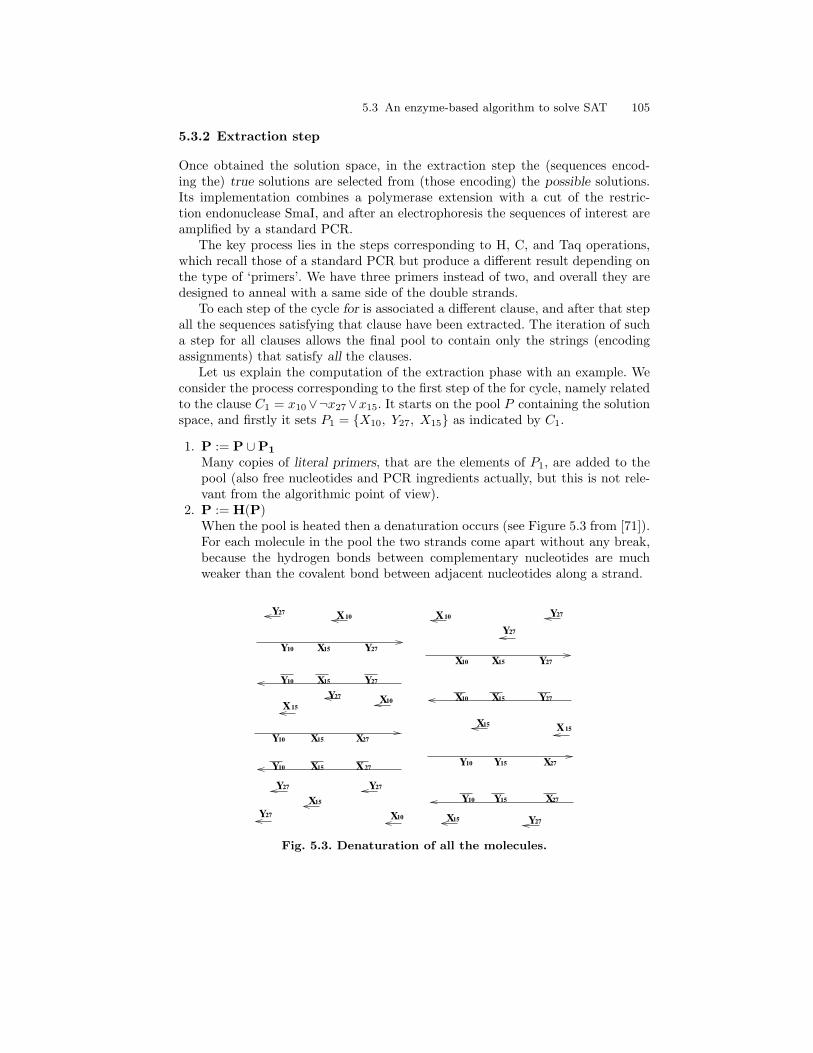
5.3 An enzyme-based algorithm to solve SAT 105
5.3.2 Extraction step
Once obtained the solution space, in the extraction step the (sequences encod-ing the) true solutions are selected from (those encoding) the possible solutions.Its implementation combines a polymerase extension with a cut of the restric-tion endonuclease SmaI, and after an electrophoresis the sequences of interest areamplified by a standard PCR.
The key process lies in the steps corresponding to H, C, and Taq operations,which recall those of a standard PCR but produce a different result depending onthe type of ‘primers’. We have three primers instead of two, and overall they aredesigned to anneal with a same side of the double strands.
To each step of the cycle for is associated a different clause, and after that stepall the sequences satisfying that clause have been extracted. The iteration of sucha step for all clauses allows the final pool to contain only the strings (encodingassignments) that satisfy all the clauses.
Let us explain the computation of the extraction phase with an example. Weconsider the process corresponding to the first step of the for cycle, namely relatedto the clause C1 = x10∨¬x27∨x15. It starts on the pool P containing the solutionspace, and firstly it sets P1 = {X10, Y27, X15} as indicated by C1.
1. P := P ∪P1
Many copies of literal primers, that are the elements of P1, are added to thepool (also free nucleotides and PCR ingredients actually, but this is not rele-vant from the algorithmic point of view).
2. P := H(P)When the pool is heated then a denaturation occurs (see Figure 5.3 from [71]).For each molecule in the pool the two strands come apart without any break,because the hydrogen bonds between complementary nucleotides are muchweaker than the covalent bond between adjacent nucleotides along a strand.
X X
X X
X
X15
1010
15
1510
Y
YY
YY27
27
27
27
27
Y10 X15 X27
Y10 Y15 X27
Y27X15X10
X15
Y10 X15 Y27
X15
YY27
Y10 15X
XY Y15 2710
X27
Y10 X15 27YX10 X15 Y27Y
27
27
X10
Fig. 5.3. Denaturation of all the molecules.

106 5 Applications of XPCR
3. P := C(P)By cooling down the pool, literal primers bind to their complementary strands,as in Figure 5.4 (which is taken from [71]).
10 Y15 X27
Y27X15X10
Y10 X15 Y27
10Y X15 Y27
15X Y27
Y10 X15 X27
X15
Y10 15Y X27
YY10 X15 X27
X10 X15 Y27
X10 X15 Y27
Fig. 5.4. Selecting by literal primers.
4. P := Taq(P)Polymerase extension elongates the double literal primers as in Figure 5.5(taken from [71]), where the resulting single strings are shown in a dots frame.
10 Y15 X27
Y27X15X10
Y10 X15 Y27
10Y X15 Y27
15X Y27
Y10 X15 X27
X15
YY10 X15 X27
X10 X15 Y27
X10 X15 Y27
Y10 Y15 X27
Fig. 5.5. Detecting of the ‘good’ assignments as single strings.

5.4 A mutagenesis algorithm 107
5. P := SmaIcut(P)Since the restriction site of SmaI is included (only) in γ, which is uniformly dis-tributed along the molecules, and since the enzyme cuts only double strandedmolecules, then after this operation only the single strings have length 1100.They encode assignments satisfying the clause C1 because contain at least oneof the literal primers in P1.The algorithm selects these single strings by means of the operation El1100(P),and then amplifies them with a PCR(α,β)(P) which restores their doublestranded form3.
The strings extracted by the first step are then filtered by the second step insuch a way that only those satisfying also the clause C2 are retained, and so onfor all the 126 clauses.
Every solution is present in the final pool, because each primer (given in manycopies) surely binds to some of its complementary regions, thus the algorithm iscomplete. Instead encoding mismatches could cause non-correctness; in fact, if aliteral primer anneals within a wrong location, then that string is selected as goodassignment even if it does not. But each solution is filtered m times, and to have anon-solution assignment in the final pool, mismatch errors should occur (selectingit) for all the clauses which it does not satisfy, and this case is quite rare.
This algorithm has been not yet experimented, thus many pitfalls could arisein the laboratory, that do not appear in the above design. However, a successfulimplementation of the first part of the algorithm just would improve the resultsobtained for the XPCR generation algorithm (presented in Chapter 4). While thelaboratory implementation of the second part could show that the extraction stepcan be performed by using only the principles of polymerase extension and bluntcuts by a restriction enzyme. With respect to [28] for example, the procedure wouldresult simpler, as no chemical synthesis and any ad hoc automated thermocyclerare required.
5.4 A mutagenesis algorithm
Mutagenesis is a very important methodology which substitute any occurrence ofa substring γ with another string δ, within the strings of a given pool. In thespecial case where α = λ we have ‘insertional mutagenesis’, that is used to blockthe expression of a gene because produces ‘mutations with lost of functionality’. Ingeneral, mutagenesis in vitro of cloned genes is the standard tool in the functionalanalysis of polymers as DNA and proteins. It may be ‘casual’ or ‘situ-specific’ (thatis site directed) mutagenesis, the first one generates mutations wherever, it is usedas a first approach to identify a functional region in a given fragment, and thesecond one is used in a second phase to analyze the functionality of a specific regionby altering its sequence. Traditionally the techniques used to perform mutagenesisare restriction enzymes or other kinds of enzymes, oligos synthesize, hybridizationand sequencing.3 From an experimental point of view, it could be better to perform electrophoresis on
double strings. For this case, electrophoresis step can be exchanged with the PCRamplification.

108 5 Applications of XPCR
In the following we present a mutagenesis algorithm based on XPCR procedurethat was introduced by Manca et al. in [150], and was implemented by the experi-ment reported in Section 6.5. Other more or less similar algorithms for mutagenesismay be found in DNA computing context, in [105] and [131] respectively.
Given in input the pool P = {αγβ}, the algorithm replaces any occurrenceof a string γ with an occurrence of the string δ, by producing in output the poolP = {αδβ}. We recall that the factor of a string α occupying from its n-th positionto its m-th position, with m ≥ n (and both smaller than or equal to the length lof α), is usually denoted by α[n,m]. One may refer to the same faction by withnegative indexes as α[n − l,m − l], meaning that we count the positions in thebackward order, from the right side to the left one of the string. Let P = {α γ β}and Q = {α[−18,−1] δ β[1, 20]}.
Mutagenesis(P, γ, δ) Algorithminput P, Q
1. split P into new P1 and P2 (with the same approximate size);
2. perform P1 := PCR(α[1,18],α[−18,−1])(P1) and P2 := PCR(β[1,20],β[−20,−1])(P2);
3. select P1 := El|α|(P1) and P2 := El|β|(P2);
4. mix the first of the obtained pools with Q, that is P1 := P1 ∪Q;
5. perform P1 := PCR(α[1,18],β[1,20])(P1);
6. select P1 := El|α|+|δ|+20(P1);
7. mix P := P1 ∪ P2;
8. perform P := PCR(α[1,18],β[−20,−1])(P );
9. select P := El|α|+|β|+|δ|(P );
output P .
If we call α1, α2 respectively the prefix and the suffix 18bp long of α, and β1, β2
respectively the prefix and the suffix of β with length 20bp, the XPCR MutagenesisAlgorithm may be depicted as in Table 5.1.
The ability to easily alter a DNA sequence allows to modify the structureof the gene products: RNA and proteins. Mutagenesis technology has changedthe way to study molecular biology, by creating the concept of ‘inverse genetics’:first one modifies the genetic sequence and then one analyzes the functionality.A consequence of this approach is the possibility to produce modifications in thenatural genetic products in such a way that they work with a better performance.In fact, protein engineering receives wide interest from the industry, especially fora likely manipulation of antibodies, that are known in detail and have an enormouspotentiality for clinical applications.

5.5 Past and future applications 109
Q := {α2δβ1} P = {αγβ}
| ⇓ split(P )
|| P1 := {αγβ} P2 := {αγβ}|| ⇓ PCR(α1,α2)(P1) ⇓ PCR(β1,β2)(P2)
|| P1 := {α} P2 := {β}
⇓ mix(Q, P1) ||
P1 := {α, α2δβ1} ||
⇓ PCR(α1,β1)(P1) ||
P1 := {αδβ1} |
⇓ mix(P1, P2)
P := {αδβ1, β}
⇓ PCR(α1,β2)(P )
P := {αδβ}
Table 5.1. XPCR Mutagenesis Algorithm transforming a pool {αγβ} into apool {αδβ}, where α = α1 · · ·α2 and β = β1 · · ·β2.
5.5 Past and future applications
In this section I would like to emphasize the impact that PCR and other biotech-nologies (such as cloning) have had in society and in other contexts than DNAcomputing, and to suggest on the way (hypothetical) future applications that PCRbased methods could have. A news article by Jean Marx quite soon documentedthe story of pivotal development of PCR [163]. In the following we report someof its main topics, together with notions and argumentations that may be foundin [231].
Many areas of biomedical and clinical microbiology research depend on theanalysis of uncommon variations in individual genes or transcripts. Modificationsof genetic sequences, such as substitution of a substring with another one, in-sertion or deletion of substrings, are called mutations. The identification and thequantification of rare mutations are objects of wide interest, as well as the studyof variations in gene sequences or transcripts in specific populations or in cellulartissues [53]. Mutations are responsible of hereditary diseases and other diseaseslike cancer, which is just implied by genetic alterations. Namely, the existence ofgenes capable to stop the tumored cells were observed together with chromoso-

110 5 Applications of XPCR
mal deletions, and such observations suggested that cells contain genes suppressorof growth that have to be inactivated before the cancer can develop. Moreover,deletions of esons are exploited for the direct diagnosis of muscular dystrophy ofDuchenne. Since the discovery of PCR, to detect or extract given DNA sequences(such as mutations) is possible and easy.
Mutations are important also because they represent the origin of the phe-notype varieties, on which is based the natural selection leading the evolution.Tissue from Egyptian mummies, or from a woolly mammoth, who last walked theSiberian steppes some 40.000 years ago, would not seem to be a likely source ofDNA for sequence analysis. After all, DNA breaks down very readily, and eventhough the mammoth had been frozen in the Siberian ice until it was chippedout, its DNA had undergone extensive degradation. With the aid of PCR though,researchers were able to produce enough mitochondrial DNA to determine the nu-cleotide sequence, because the DNA to be amplified by PCR does not have to bein good shape. The results showed, not surprisingly, that the mitochondrial DNAof this extinct species is very similar to that of the modern elephant, its closerelative. Variations in DNA structure were also used to trace evolution of humanpopulations. For example, a particular mutation was identified, a 9bp deletion, inhuman mitochondrial DNA that apparently originated in East Asia. It can aid intracking the migrations of ancient peoples, namely, the finding of the 9bp deletionin some American Indians and in New Guineans indicates that migrants form EastAsia contributed to the founding of these populations.
This opened the way to a variety of applications of PCR technique in addi-tion to analyzing ancient DNA samples. One which has advanced very rapidly wasthe forensic use of the technology to identify (or exonerate) suspects in rape andmurder cases. The biological evidence found at the scene of violent crimes, includ-ing bloodstains, semen, and hair, is often of such a poor quantity or quality thatit cannot be analyzed by other forensic techniques. The DNA is thus amplifiedand then compared with the suspected person’s DNA to obtain an identification.Moreover, polymorphic loci exist along the protein polymers that can be uniquelyassociated to a single individual (the test is called DNA fingerprinting).
PCR was also applied in clinical medicine as a gene amplification technique.It is used, for example, to simplify and speed up the prenatal diagnosis of geneticdiseases, including β-thalassemia and sickle cell anemia, to detect viral infections,including AIDS, to do the tissue typing needed for matching the donors and recip-ients of transplanted organs, and to identify the genes that confer susceptibility toautoimmune diseases. These diseases, which are caused by an abnormal attack ofthe immune system on the body’s own tissues, actually are not classified as geneticdiseases. They have a genetic component, however, in that susceptibility to manyof the diseases has been linked to particular variants of a specific class of molecules,that mediate the immune cell interactions necessary for mounting normal immuneresponses. By allowing the rapid amplification and sequencing of genes, the PCRtechnique also facilitated the studies needed for a better understanding of geneticcontributions to autoimmunity.
Still in immunological context, DNA generation methods could be importantto study rearrangements of antibody genes. Some organisms have enzymes thatare able to recombine the ‘ipervariable’ regions of antibodies in such a way that
5.5 Past and future applications 111
cells can defend from an external attack of pharmacies or of virus. This processis crucial to understand how the immunological response works and how cellsdevelop a specific resistance to some pharmacies. Experiments have been carriedout, where substrates generated by artificial recombination were put in cells, suchas fibroblasts and lymphocytes B, then treated with some pharmacy. The survivingcells have been those capable to develop a resistance to the pharmacy. Such aresistance was induced by the enzyme able to recombine the artificial substrate.Finally, from human lymphocyte B was extracted, cloned, and studied, the DNAsegment responsible of such a recombination, and it resulted to contain two specialgenes that cooperate to activate the recombination of antibodies’ portions withhigh efficiency.
XPCR extraction on the other hand, has the potentiality to be really usefulto detect mutant gene segments. For example, in some forms of hereditary cancer,cloned genes may be used to determine whether the components of a family areunder risk to have cancer. An extraction method applied on the DNA from cells ofthe familiars could point out the presence of a specific gene. The high sensitivity ofthe PCR, and the extraction methods based on PCR, also make it well suited fordetecting viruses, especially those viruses that go underground in infected persons,often persisting for several years in a small number of cells before causing obvioussymptoms of disease. Human immunodeficiency virus type I (HIV-1), the AIDSvirus, is a case in point. AIDS has a latent period of several years, and very fewsusceptible cells (perhaps 1 in 10.000) actually carry the virus. Nevertheless PCRis used to amplify HIV-1 gene sequences in the DNA of peripheral blood cells frominfected individuals, thereby allowing the direct detection of the viral presence;it was shown that PCR is able to pick up one to ten copies of viral DNA per 1million of cells!
PCR technique, by making easier the detection of HIV-1, facilitates the epi-demiological studies needed to resolve the issue of whether the virus persists in allantibody-positive individuals, or whether it may sometimes be eliminated by theimmune system. For clinical purposes, it is possible to use PCR to estimate howmuch HIV-1 a person carries. Individuals with the larger virus burdens, who arepresumably at high risk of coming down with AIDS, might then be candidates forearly drug therapy. In addition, the technique might help to determine whether acandidate antiviral drug actually reduces the mount of virus carried by patientsundergoing therapy.
5.5.1 Support to cancer research
The study of recombinant DNA has been essential in the progress for the diagnosisof cancer. PCR is also aiding efforts to track down the cellular changes that playa role in cancer development. For example, the normal genes that control cellgrowth and differentiation may sometimes undergo alterations that convert themto cancer-causing genes, called oncogenes. For some genes, such as ras, a changein a single base pair is sufficient to do this. Determining how frequently ras geneactivation might contribute to the development of human cancers has been difficult.Although ras oncogenes have been found in several types of human cancers, in moststudies, the percentage of tumors carrying the active oncogene was low, 10% or

112 5 Applications of XPCR
less. This figure may have been so low at least partly because identifying pointmutations, such as those causing ras gene activation, could be difficult. While usingPCR, more than a third of human colon cancers was shown carry oncogenic rasmutations. Similar approaches showed that cancer cells from about one quarter ofpatients with acute myelitis leukemia also contain ras oncogenes.
When patients undergo surgery for cancer, samples of the tissue removed areembedded in paraffin blocks. This is done so that thin tissue slices can be madeand then examined by a pathologist to confirm the cancer diagnosis. The blocksof paraffin-embedded tissue are usually kept so that there may be a worldwidecollection of such preserved tissue specimens, with defined pathologies and knownclinical results for the patients. DNA sequences of the human papilloma virus wasdetected in samples of cervical cancer tissue with the aid of the PCR, even thoughthe tissue preparations had been made years ago and the DNA is likely to bedegraded. The most important consequence of this work was that it opened upthe possibility of using the tissue specimen collection for studies aimed at tracingthe contributions of viruses and oncogenes to cancer development.
5.5.2 Ethical aspects
In 1971, while the first genetic cloning experiments were being made, some anxietyarose about the safety of such a kind of experiments. Communities were worriedespecially about the cloning of genomes of tumored virus and the replicating ofthe molecules in bacterial cells such as Escherichia Coli, because of the possibilityto transmit human cancer by means of these bacteria. At that time though, theydid not have the data necessary to evaluate the actual risks4.
The signatories of the 1974 Berg letter to Science5 had made a principled publicappeal for biologists to hold off doing two specific types of recombinant experi-ment and to weigh the possible consequences of others, until the correspondingrisks will have been clearer. Such an evaluation was done in February of 1975 bymore than 100 famous molecular biologists, in the Conference Center of Asilomar,at Monterey, California. The issues at Asilomar were clearer than those that aroselater. They gathered many proposals, and one of them was to use only geneticallyenable bacteria to clone DNA, so that they could grow only in vitro6. These direc-tives were followed and formalized by a special committee nominated by NationalInstitutes of Health (NIH) in USA, that in particular prohibited experiments ongenes from tumored virus. In July 1976 the current indications were rectified by aRecombinant DNA Advisory Committee (RAC) constituted also by non-scientistsand lowers. The European formulation of such a mobilization was the GeneticManipulation Advisory Group (GMGA), in England. More data and further ex-
4 M. Singer and D. Soll. Guidelines for DNA hybrid molecules, Science, 181:1174, 1973.5 P. Berg, D. Baltimore, H. W. Boyer, S. N. Cohen, R. W. Davis, D. S. Hogness, D.
Nathans, R. Roblin, J. D. Watson, S. Weissman, and N. D. Zinder. Potential biohazardsof recombinant DNA molecules. Science. 185(148):303, Jul 26, 1974.
6 P. Berg, D. Baltimore, S. Brenner, R. O. Roblin, and M. F. Singer. Asilomar conferenceon recombinant DNA molecules, Science, 188:991-994, 1975.

5.5 Past and future applications 113
periments convinced the NIH to admit the cloning of tumored virus genes, inJanuary of 19797.
Nowadays research performed by DNA manipulation techniques is extraordi-narily growing. The application to the pharmacy production and vaccines gavebirth to the biotechnological industry. The technological progress about geneticcloning, genetic structure and expression, and human genetics, of the last twentyyears has no comparison with the knowledge we had accumulated in the previoustimes, and PCR was definitely a milestone in such an advancement.
Synthetic proteins are made for facing different pathologies, like cancer, aller-gies, autoimmune diseases, neurological disturbs, cardiopathologies, hematologicalalterations, genetic infections and diseases, production of soap and food! Very in-teresting examples of recombinant pharmacy produced by genetic engineering arethe human insulin, which is the hormone regulating the sugars metabolism, thehuman Growth Hormone, the Hepatitis B vaccine, and a rational projecting ofpharmacies.
Section 5.1 and Section 5.3 include respectively more or less wide parts of thefollowing papers:
• G. F., Hard Instances of SAT, TR of the project ‘Biomolecular algorithms forNP-Complete problems’, Department of Computer Science, University of Pisa,July 2002.
• G. F., A Polymerase Based Algorithm for SAT, M. Coppo and E. Lodi and G.M. Pinna, editors, Theoretical Computer Science, Lecture Notes in ComputerScience 3701, Springer, pp 237-250, October 2005.
7 Department of Health, Education, and Welfare. Legislation, Regulations, or Statutesfor Previous U.S. Bioethics Initiatives, Federal Register, January 11, 1979.

6
Laboratory Experiments
There is no higher or lower knowledge, but one only,flowing out of experimentation.
Leonardo da Vinci
Three laboratory experiments validating respectively the extraction (Sec-tion 3.4), recombination (Section 4.1) and mutagenesis (Section 5.4) algorithmsare reported in the last sections. The first two ones have been designed and di-rected entirely by myself, the third one just partially (at that time I was spendingfew months at University of South Florida). I have not used any design servicefor the encodings, just ad hoc variants of results from the literature (for exam-ple, [8, 29, 114]) and some checking by means of a program, which given a coupleof sequences finds common subsequences having length greater than five. This hasbeen an useful information to avoid mismatches, especially in our cases wherePCRs have been often performed at low (under suggested limits) temperatures.
The trials are presented according to their chronological order, so that thereader can notice as the experimental tricks (about preferred lengths, meltingtemperatures and annealing specificity) and the tested sequences from one experi-ment were rearranged for the next one. The experiments were manually carried onby Cinzia Giagulli, who is a postdoc researcher from the Department of GeneralPathology of University of Verona. Initially I was thinking that the main difficultyto set up an experiment with her would have been to find a common languageto exchange ideas, a simple manner to explain an algorithm and its (theoretical)implementation and to understand the technical ways to perform the required op-erations. But quite soon I have crashed into a totally different reality, and I endedup with as unexpected as practical problems. Section 6.2 reports what I noticedduring my visits in the laboratory. Apart mismatching problems studied in the lit-erature and partially described in Section 3.5, indeed many other (more practical)problems can be avoided by ‘good’ encodings design. One studies on the booksabout the difference between the (weaker) bonds A-T and the (stronger) bondsC-G, but usually he/she does not realize how much this difference influences themelting temperature of the sequences (connected to the percentage of C-G base

116 6 Laboratory Experiments
pairs) and the formation of secondary structures. One studies as well that theagarose gel for electrophoresis can be made more dense in order to discriminatethe shortest strings, but there are not reported the manual difficulties to man-age a 5% gel with respect to a 3% one. These are just examples of the fact thatthere have been a lot of factors hidden behind the passage from the algorithmsexplained in the previous chapters to their laboratory implementation describedin the following.
Firstly, I realized that after the theoretical design of a DNA algorithm andbefore starting to talk about implementation, one has to submit the algorithminto the following constraints:
• Maximum length of (initial) sequences to order from a company has to be150bp. In our case sequences shorter than or equal to 100bp have been finallypreferred, while very long sequences to work with have been extracted fromhuman gene RhoA.
• Lengths of primers (to use during PCRs) have to be from 17 to 30 bp. Currentlywe are doing an experiment with primers 20 long, that’s the best choice.
• Primers should have a balanced distribution of C-G and A-T base pairs. Theyneed to be with no internal secondary structure and with no complementar-ity between their 3′ ends (otherwise they anneal each other, forming ‘primer-dimers’).
• Primers must have comparable melting temperatures (ranging from 55 to 70Celsius degrees), and they should start and end with a C or a G, in order toallow specific annealing.
• All sequences that are separated by electrophoresis should have length at least50bp
The first constraint is related to economic and attendance time reasons, thelast one to the feasibility to work with gel 3%, and the middle ones to biochemicalfactors. In most PCR applications, it is the sequence and the concentration of theprimers that determine the overall assay success. Melting temperature of primersis thus something to take strictly in account during the encoding phase in orderto perform specific PCRs during the experiment. Section 6.1 explains with moredetails how it is calculated.
6.1 Melting temperature
By definition, the temperature at which 50% of a given oligonucleotide is hy-bridized to its complementary strand is called melting temperature, shortly Tm.
The melting temperature characterizes the stability of the double DNA fila-ments formed between an oligonucleotide and its complementary strand. It is veryimportant for determining the optimal temperature at which to use an oligonu-cleotide as a primer in PCR applications (annealing temperature), or in generalas a probe for in situ hybridization.
In the absence of destabilizing agents, like formamide or urea, Tm will dependon three major parameters:

6.1 Melting temperature 117
1. The sequence: a GC-rich sequence has a higher melting temperature.2. The strand concentration: high oligonucleotide concentrations favor paired for-
mation, which results in a higher melting temperature.3. The salt concentration: high ionic strength results in a higher Tm because
cations stabilize the DNA duplexes.
Many methods have been proposed to empirically determine Tm values. Foroligonucleotides s having length at most 20 bases, we used the following classi-cal calculation for melting temperature, according to the Wallace rule for shortoligonucleotides
Tm(s) = 2(|s|A + |s|T ) + 4(|s|G + |s|C)
where |s|N denotes the number of occurrences of the symbol N in the sequence s.In the case of longer DNA fragments, the nearest-neighbor method [30, 212],
which combines solid thermodynamics and experimental data, offers a reliable es-timation of the Tm. In the nearest-neighbor formula, the two parameters affectingthe Tm value are the salt concentration and the concentration of single strandedDNA. These two experimental variables are here chosen in order to optimize DNAamplification by PCR and their values are fixed at 50 mM (millimoles) of salt and250 pM (picomoles) of oligonucleotide, as suggested in [205].
The formula to calculate the Tm by the nearest-neighbor method is
Tm = H(A+ S) +R ln(Ct/4)273.15 + 16.6 log(P ),
where
• H is the sum of the nearest-neighbor enthalpy changes for hybrid formation (itis a negative value, estimated in cal per mole).
• A is a constant for helix initiation. It is equal to -10.8 (cal. per mole) fornon-selfcomplementary sequences and - 12.4 for selfcomplementary sequences.
• S is the sum of the nearest-neighbor entropy changes for paired formation (itis a negative value, estimated in cal per mole).
• R is the molar gas constant (1.987 cal per mole).• Ct is the total molar concentration of strands when oligonucleotides are not
self complementary. It is equal to 4 times this concentration in the case ofselfcomplementary sequences.
• P is the salt concentration.
The Tm value is calculated for phosphodiester oligonucleotides used in DNA-amplification experiments. Even though this calculation does not take into accountany nucleotide modification, like biotin, digoxigenin, fluorescent dyes, it still givesus a good estimate of the starting conditions.
Coming back to our experiments, the melting temperatures of the primersinvolved in each PCR have been made close each other, and the correspondingPCR was then performed by setting the lowest temperature in order to makemore specific the primer annealing step.
118 6 Laboratory Experiments
6.2 In a laboratory
Let us assume for example that we want to implement the following simple algo-rithm, starting from a pool of 1011 molecules, with four kinds of sequences S1, S2,S3, S4 uniformly distributed, having the same length (100bp), the same prefix αand the same suffix β.
1. Take randomly 100 molecules2. Amplify them by PCR(α, β)3. Check the amplification product by electrophoresis.
First of all we have to set up a solution containing 1011 molecules. We have thetest tubes arrived from the company, each of them contains a different sequencefrom {S1, S1, S2, S2, S3, S3, S4, S4}, with a concentration of 100 µmoles (a moleis 106 micromoles) per liter. Since we can take just prefixed quantities of solutionby means of tared pipettes1, some counts are necessary in order to know how totake 1011 and then 100 molecules from a solution.
Since the sequences have to be uniformly distributed we need to take 1011/8=12,5 109 molecules from each test tube. The following proportions (6, 022 1023 isthe Avogadro number) indicate (by X) how many micromoles we have to take ofeach sequence in how many microliters (Y) of solution.
1mole : 6, 022 1023 molecules = X : 12, 5 109moleculesX = 2, 075 10−14 moles = 2, 075 10−8µmoles
100 µmoles : 1L = 2, 075 10−8µmoles : YY = 2, 075 10−10L = 0, 0002075 µl
Y is definitely lower than 0.2 µl, which is the minimum we are able to take witha pipetman. If we put (by a P2 pipette for example) 1 µl of each sequence into100 µl of sterile water, and from this solution we transfer 1 µl into 100 µl of sterilewater, then we can take (by a P10) 2,075µl from the solution that corresponds to12.5 109 molecules of each sequence. Here we have preferred to dilute two times
1 Main tools to handle liquids.
1. Accurate and precise, ideal for molecular biology techniques (PCR, DNA sequencing)• P2 (capturing from 0.2 µl to 2 µl)• P10 (capturing from 1 µl to 10 µl).
2. Suited for small-volume dispensing of aqueous fluids of moderate viscosity and den-sity (molecular biology, immunology)• P20 (capturing from 2 µl to 20 µl)• P100 (capturing from 20 µl to 100 µl)• P200 (capturing from 50 µl to 200 µl)• P1000 (capturing from 200 µl to 1000 µl).
3. Ideal for large-volume dispensing of aqueous fluids of moderate viscosity and density.• P5000 (capturing from 1000 µl to 5000 µl)• P10ml (capturing from 1 ml to 10 ml).
6.2 In a laboratory 119
in 100 µl instead of diluting once in 1000 µl and then taking just the minimumpossible (around 0.2 µl). This is the experimental way to proceed, one has alwaysto be aware that we are dealing with inexact estimations and instruments.
By taking 2,075µl from the solution corresponding to every sequence, we reach16.6 µl of solution which we round by adding 993,4 µl of sterile water. Thus weobtain 1011 molecules uniformly distributed in 1ml of solution. To select randomly100 molecules starting from 1011 molecules in 1000 µl, it is enough to dilute anal-ogously as above, by taking 1 µl from the current solution and putting it into 1000µl of water for two times. Next step is to amplify such 100 molecules (with a sameprefix α and a same suffix β) by polymerase chain reaction.
6.2.1 PCR protocol
PCR is an in vitro method for enzymatically synthesizing defined sequences ofDNA. The reaction uses two oligonucleotide (called primers), that hybridize tothe opposite strands of the DNA which has to be amplified in their terminal parts.The elongation of the primers is catalyzed by Taq enzyme, which is a heat-stableDNA polymerase that is isolated from the thermophiliac eubacterium Thermusaquaticus.
PCR was originally performed with a DNA polymerase from the bacteriumEscherichia Coli, but this enzyme is inactivated by the high temperatures neededfor strand separation, whereas the primary requirements for a polymerase used inthe PCR are good activity at temperatures around 75◦C and ability to retain thatactivity after prolonged incubations at even higher temperatures (95◦C). There areat least three DNA polymerases (Taq, Tth, Pwo) which meet those requirements,but Taq is the most efficient. It has a half life of less than 5 minutes at 100◦C,however, the enzyme retains its activity for much longer times (half life up to40 minutes) at 95◦C. The high processing, absence of exonuclease activity, andtemperature optima of Taq DNA Polymerase make the enzyme useful even forDNA sequencing, especially where the resolution of secondary structures playsa major role. Moreover, this Polymerase has the advantage to accept modifieddeoxyribonucleotide tri-phosphates as substrates, and can be used to label DNAfragments either with radio nucleotides, digoxigenin, biotin, or fluoresce.
A repetitive series of cycles involving template denaturation, primer anneal-ing, and extension of the annealed primers by Taq DNA Polymerase results inexponential accumulation of a specific DNA fragment. In fact, since the primerextension products synthesized in a given cycle can serve as a template in the nextcycle, then the number of DNA copies approximately doubles every cycle: thus,20 cycles of PCR yield about a million copies (220) of defined DNA.
There exist standard protocols to perform PCR, however, in principle, eachphysical and chemical component can be modified to produce a potential increasein yield, specificity or sensitivity, and these factors are not independent of eachother. It follows a description of how a PCR(α, β) was performed in our laboratory.
We have a termocycler to set, an electric vortex to mix solutions, a refrigeratorcontaining the test tubes of the DNA sequences and of the PCR ingredients, and allthe pipettes and differently sized test tubes within easy reach. We start by cleaning
120 6 Laboratory Experiments
the counter carefully, and by wearing fresh gloves. In fact, the ability of the PCR toamplify a single molecule means that trace amounts of DNA contaminants couldserve as templates, resulting in amplification of the wrong template (false positive).
Firstly, the PCR mixture has to be prepared for three2 samples of 50 µl, withthe following ingredients.
• Buffer of PCR (10x, meaning that it is initially 10 times concentrated). It isa transparent liquid having saline concentration and PH such that the phys-iological environment of the cell is simulated, thus the enzyme can work asusual.
• Taq DNA Polymerase. For most assays, the optimum amount of it is between0.5 and 2.5 units (we used 1.25 units). Increased enzyme concentrations some-times lead to decreased specificity.
• dNTP mixtures. If the concentration of the four dNTPs is imbalanced, this canreduce Taq fidelity. We used an amount of 200 µM .
• MgCl2. It is a necessary ingredient to catalyze the enzyme action, and itsoptimal concentration may vary from approximately 0.5 mM to 5 mM, thestandard value is 1.5mM. Magnesium influences enzyme activity, increases theTm of double stranded DNA, and forms soluble complexes with dNTPs toproduce the actual substrate that the polymerase recognizes.
• Primer concentrations between 0.1 and 0.5 µM are generally optimal (we havetaken 0.5 µl of α and 0.5 µl of β). Higher primer concentrations may promotemis-priming and accumulation of unspecific product. Lower primer concentra-tions may be exhausted before the reaction is completed, resulting in loweryields of desired product.
• DNA template. The primer/template ratio strongly influences the specificity ofthe PCR and should be optimized empirically. With a small amount of templatethe primers may not be able to find their complementary sequences, whereastoo much template may lead to an increase in mis-priming events. The purityof template also influences the outcome of the reaction.
We used ice to which insert test tubes during the preparation of such a mixture,in order to avoid unspecific formations, and pipettes instead of vortex to mix thesolution once the Taq was in the solution (otherwise foam could be produced).The PCR program was then set as in the next points.
• Initial denaturation (at temperature 95◦ C).It is very important to denature the template DNA completely. Initial heatingof the PCR mixture for few minutes (we set 4) at 95◦ C is enough to completelydenature complex genomic DNA, so that the primers can anneal to the templateas soon as the reaction mix is cooled. If the template DNA is only partiallydenatured, it will tend to ‘snapback’ very quickly, preventing efficient primerannealing and extension or leading to ‘self-priming’, which can lead to falsepositive results.
2 We take two extra samples called control reactions: the negative one, which containsall reaction components except the primers, and the positive one, which contains allreaction components with a different DNA template. They are useful to check that thereaction components are good and work well, in fact, no amplification is expected forthe negative control, and a different amplification is expected for the positive control.

6.2 In a laboratory 121
The denaturing step is performed (at temperature 95◦C) initially for longertime, and then repeated for some seconds (we set 30) at the beginning of everycycle, to avoid that an incompletely melted DNA snaps back, thus giving noaccess to the primers.
• Primer annealing.Temperature for this step has to be optimized empirically, we have chosen toset the lowest between the melting temperatures of the primers α and β (thatis calculated as explained in Section 6.1) for one minute.The choice of the primer annealing temperature is probably the most criticalfactor in designing a high specificity PCR. If the temperature is too high, noannealing occurs, but if it is too low, unspecific annealed products increasedramatically. If a primer has a 3′ end which anneals to any site on a tem-plate, irrespective of whether it anneals specifically or not, the primer will beelongated from that 3′ end. Also, at low temperatures, primers may hybridizepartially without involving their 3′ end, and such hybrids will not be extended.
• Primer extension.It is normally carried out at temperature 72◦ C, that is ideal for Taq DNAPolymerase working (at 72◦ C it can add 60 bases per second!). Usually a 20second extension is sufficient for fragments shorter than 500bp and a 40 secondextension is sufficient for fragments up to 1.2Kb. However, these times mayvary (for sequences 100 long we set 10 seconds as duration of this step).
• Cycles number.In an optimal reaction, less than 10 template molecules can be amplified inless than 40 cycles to a product that is easily detectable on an ethidium bro-mide stained gel (see Section 6.2.2). Most PCRs should, therefore, include only25 to 35 cycles. As cycle number increases, unspecific products can accumulate.
• Final extension.Usually, after the last cycle, the reaction tubes are held at 72◦ C for 5-15minutes to promote completion of partial extension products and annealing ofsingle stranded complementary products.
From a biotechnological point of view, main limitations of PCR are:
• One only obtains a DNA fragment. To see this DNA at work inside a livingorganism, some type of cloning has to be done.
• Only relatively short sequences can be amplified reliably. Anything more than10,000 base pairs is unlikely to be amplified.
• One needs to know the right primer sequences to use, at both ends of thesequence you want to amplify. If two related genes have the same end sequences,one might amplify the wrong gene.
• The possibility of mis-incorporation of dNTP, which arises from the polymerasecharacteristics, must be taken in consideration.
Let us assume we are at the end of the second step of the algorithm: we justamplified by 35 cycles of PCR(α, β) 100 molecules containing four kinds of se-

122 6 Laboratory Experiments
quences S1, S2, S3, S4 uniformly distributed (having the same length, the sameprefix α and the same suffix β).
Before of carrying on an electrophoresis to verify that the amplification hap-pened correctly (we expect to see amplified sequences all 100 long), we check thatour amount of DNA is enough to be detected by electrophoresis. On an agarosegel, the limit of visibility is 50ng of DNA, and we want to be sure to put, say,100ng of DNA in the gel.
We recall that 100 ng = 10−7gr, and that the number of moles of a substanceis given by the rate of its weight to its molecular weight. The molecular weight ofeach DNA sequence is known, it depends on that of its bases and on its length. Infact, the molecular weights of the four nucleotides are not identical (phosphatesand sugars are a constant but bases have different weights), but in routine work weusually average the molecular weights of all four bases and go with 324.5 Daltonper DNA nucleotide (that means 324.5 grams/mole of individual nucleotides3), anda corresponding base pair weight of 649 Dalton. For our sequences S1, S2, S3, S4,we computed the molecular weight average of 246700 : 4 = 61675 g/m.
10−7g : 61675 g/m = 1, 621403 10−12 moles1mole : 6, 0221023 molecules = 1, 62140310−12 moles : XX = 9, 7640888661011 molecules
These counts allow to know that 100 ng of DNA approximately correspond to9,764088866 1011 molecules. Since after forty cycles of PCR on 100 molecules weshould have about 100 240 = 109.951.162.777.600 molecules in 56 µl of solution(50 from the PCR mix plus 6 of dye), we can easily compute how much solution(Y) is enough to upload to have 100 ng of DNA in the gel.
109.951.162.777.600 molecules : 56µl = 9, 764088866 1011 molecules : YY = 0, 249µl
We usually upload 15 µl of solution in each well of the gel.
6.2.2 Gel-electrophoresis
The gel-electrophoresis technique, that separates DNA molecules by their length,is simple, rapid to perform, and capable of resolving fragments of DNA that cannotbe separated adequately by other procedures. Since the DNA is negatively charged,after being placed in a small well of a gel in an active electric field, it slowly movestowards the positive side. Larger (heavier) molecules move slower and smallermolecules move faster. More precisely, they migrate through gel matrices at ratesthat are inversely proportional to the logarithm (of basis 10) of their length. Largermolecules have greater frictional drag, they worm the way through the pores of thegel less efficiently than smaller molecules. After a while the electric field is stopped,and the portion of the gel that contains molecules with the desired length can becut out of the gel, DNA purified, and then used in subsequent experiments. Besides,the location of DNA within the gel can be determined directly by staining with lowconcentrations of the fluorescent intercalating dye ethidium bromide, and bands3 In other words, a mole of one base weighs approximately 325 g.
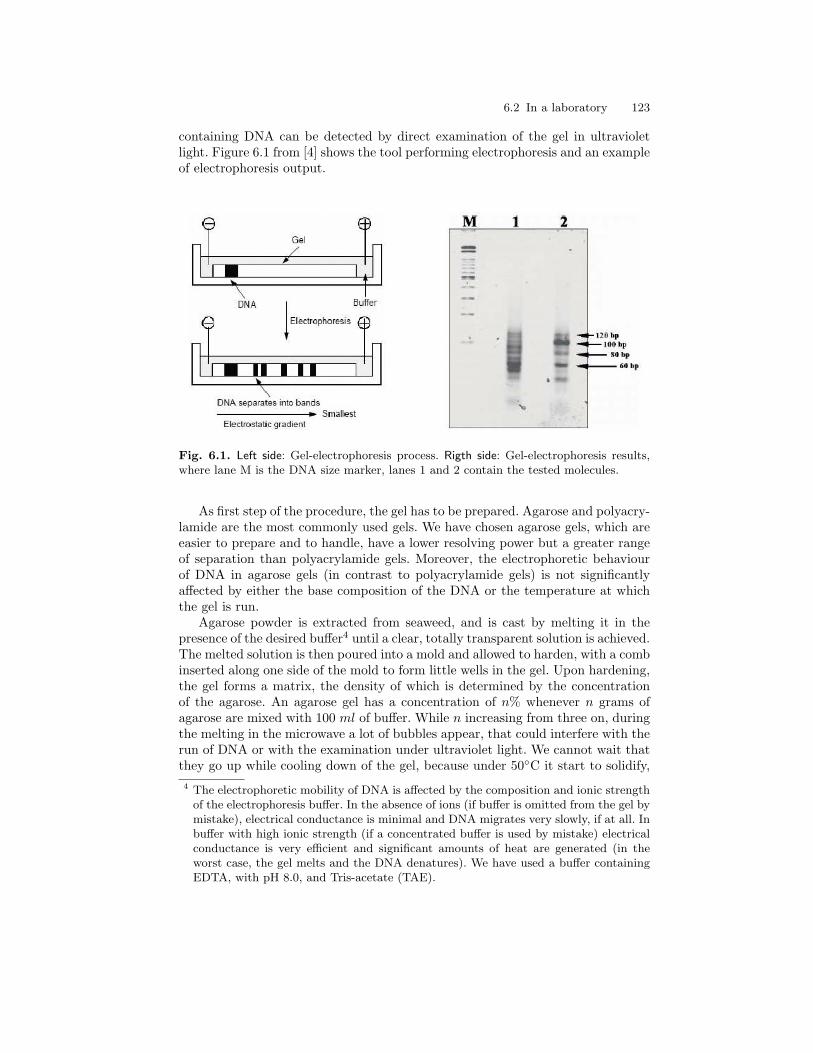
6.2 In a laboratory 123
containing DNA can be detected by direct examination of the gel in ultravioletlight. Figure 6.1 from [4] shows the tool performing electrophoresis and an exampleof electrophoresis output.
Fig. 6.1. Left side: Gel-electrophoresis process. Rigth side: Gel-electrophoresis results,where lane M is the DNA size marker, lanes 1 and 2 contain the tested molecules.
As first step of the procedure, the gel has to be prepared. Agarose and polyacry-lamide are the most commonly used gels. We have chosen agarose gels, which areeasier to prepare and to handle, have a lower resolving power but a greater rangeof separation than polyacrylamide gels. Moreover, the electrophoretic behaviourof DNA in agarose gels (in contrast to polyacrylamide gels) is not significantlyaffected by either the base composition of the DNA or the temperature at whichthe gel is run.
Agarose powder is extracted from seaweed, and is cast by melting it in thepresence of the desired buffer4 until a clear, totally transparent solution is achieved.The melted solution is then poured into a mold and allowed to harden, with a combinserted along one side of the mold to form little wells in the gel. Upon hardening,the gel forms a matrix, the density of which is determined by the concentrationof the agarose. An agarose gel has a concentration of n% whenever n grams ofagarose are mixed with 100 ml of buffer. While n increasing from three on, duringthe melting in the microwave a lot of bubbles appear, that could interfere with therun of DNA or with the examination under ultraviolet light. We cannot wait thatthey go up while cooling down of the gel, because under 50◦C it start to solidify,4 The electrophoretic mobility of DNA is affected by the composition and ionic strength
of the electrophoresis buffer. In the absence of ions (if buffer is omitted from the gel bymistake), electrical conductance is minimal and DNA migrates very slowly, if at all. Inbuffer with high ionic strength (if a concentrated buffer is used by mistake) electricalconductance is very efficient and significant amounts of heat are generated (in theworst case, the gel melts and the DNA denatures). We have used a buffer containingEDTA, with pH 8.0, and Tris-acetate (TAE).

124 6 Laboratory Experiments
therefore such bubbles have to be taken away from the mold manually. Anotherthing to keep in mind is that any next time the gel is melted little part of thebuffer will evaporate, and the concentration of the gel will increase. A linear DNAfragment of a given size migrates at different rates through gels containing differentconcentrations of agarose. There is a linear relationship between the logarithmof the electrophoretic mobility η of DNA and the gel concentration τ , which isdescribed by the equation:
log η = log η0 −Krτ
where η0 is the free electrophoretic mobility of DNA and Kr is the retardationcoefficient, a constant that is related to the properties of the gel and the sizeand shape of the migrating molecules. Approximately, we need a concentration ngreater than 3 for lengths shorter than 100 (n = 4 for lengths 50-100 and n = 5for lengths 20-50).
In order to detect the DNA bands, in the gel it is added 0.5 mg/ml of ethidiumbromide5, a fluorescent dye which intercalates between stacked base pairs. If theconcentration is too high, then under the ultraviolet light the gel will result all overstained. Some loading buffer and colouring is instead added to the DNA solutionrespectively to make it heavier (in order to stay in the well) and visible duringthe run. One should be careful to the cases where sequences run as fast as thecoloring, because the coloring could then cover the signal. A crucial point is toload a marker in a lateral well of the gel. A marker of 25bp for example6 containsfragments of 25, 50, 75, 100 bp and so on until 200 bp. It is used as calibrationpath: different bands on this path mark known lengths, and the location of bandson other paths is compared with this calibration path (see rigth side of Figure 6.1)
At this point the gel is ready and the electric field can be switched on. We set100 volt x 400 milliampere x 20 minutes. This choice is determined by experience(with such tools) and by the Ohm equation. We recall that in an electric fieldthe electricity I is proportional to the difference of potential V by a coefficientdepending on the means resistance R as
I =V
R
The point here is to set V high enough that the field remains uniform during thewhole electrophoresis.
The system has to be stopped approximately when the sequences (visible bythe coloring) reach an half of the maximum distance, by occupying an half of thegel container. In fact, if we stop before, the strings could be not yet separated, andif we stop after, the shortest strings would stay in a portion of gel without ethidiumbromide (which run in the opposite direction of DNA!) and could not be detectedby ultraviolet light. After we switch off the field we can see and photograph thesignal. Imagines are obtained as those reported in the following of this chapter.
5 It is a powerful mutagen, is carcinogen and should be handled with care!6 It could be a marker of 50bp or 10bp, respectively starting from strings long 50, or
100, and going ahead with differences of 25bp.
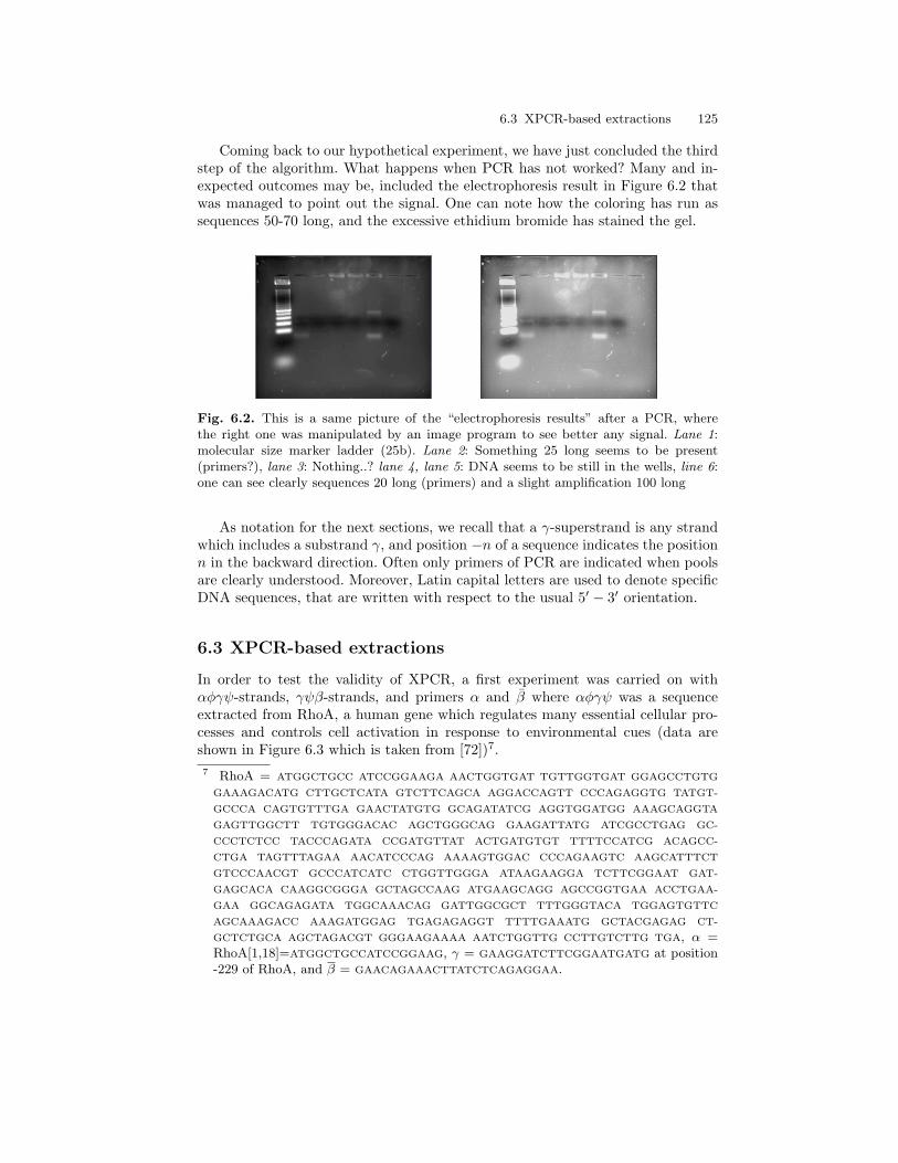
6.3 XPCR-based extractions 125
Coming back to our hypothetical experiment, we have just concluded the thirdstep of the algorithm. What happens when PCR has not worked? Many and in-expected outcomes may be, included the electrophoresis result in Figure 6.2 thatwas managed to point out the signal. One can note how the coloring has run assequences 50-70 long, and the excessive ethidium bromide has stained the gel.
Fig. 6.2. This is a same picture of the “electrophoresis results” after a PCR, wherethe right one was manipulated by an image program to see better any signal. Lane 1:molecular size marker ladder (25b). Lane 2: Something 25 long seems to be present(primers?), lane 3: Nothing..? lane 4, lane 5: DNA seems to be still in the wells, line 6:one can see clearly sequences 20 long (primers) and a slight amplification 100 long
As notation for the next sections, we recall that a γ-superstrand is any strandwhich includes a substrand γ, and position −n of a sequence indicates the positionn in the backward direction. Often only primers of PCR are indicated when poolsare clearly understood. Moreover, Latin capital letters are used to denote specificDNA sequences, that are written with respect to the usual 5′ − 3′ orientation.
6.3 XPCR-based extractions
In order to test the validity of XPCR, a first experiment was carried on withαφγψ-strands, γψβ-strands, and primers α and β where αφγψ was a sequenceextracted from RhoA, a human gene which regulates many essential cellular pro-cesses and controls cell activation in response to environmental cues (data areshown in Figure 6.3 which is taken from [72])7.7 RhoA = ATGGCTGCC ATCCGGAAGA AACTGGTGAT TGTTGGTGAT GGAGCCTGTG
GAAAGACATG CTTGCTCATA GTCTTCAGCA AGGACCAGTT CCCAGAGGTG TATGT-
GCCCA CAGTGTTTGA GAACTATGTG GCAGATATCG AGGTGGATGG AAAGCAGGTA
GAGTTGGCTT TGTGGGACAC AGCTGGGCAG GAAGATTATG ATCGCCTGAG GC-
CCCTCTCC TACCCAGATA CCGATGTTAT ACTGATGTGT TTTTCCATCG ACAGCC-
CTGA TAGTTTAGAA AACATCCCAG AAAAGTGGAC CCCAGAAGTC AAGCATTTCT
GTCCCAACGT GCCCATCATC CTGGTTGGGA ATAAGAAGGA TCTTCGGAAT GAT-
GAGCACA CAAGGCGGGA GCTAGCCAAG ATGAAGCAGG AGCCGGTGAA ACCTGAA-
GAA GGCAGAGATA TGGCAAACAG GATTGGCGCT TTTGGGTACA TGGAGTGTTC
AGCAAAGACC AAAGATGGAG TGAGAGAGGT TTTTGAAATG GCTACGAGAG CT-
GCTCTGCA AGCTAGACGT GGGAAGAAAA AATCTGGTTG CCTTGTCTTG TGA, α =RhoA[1,18]=ATGGCTGCCATCCGGAAG, γ = GAAGGATCTTCGGAATGATG at position-229 of RhoA, and β = GAACAGAAACTTATCTCAGAGGAA.
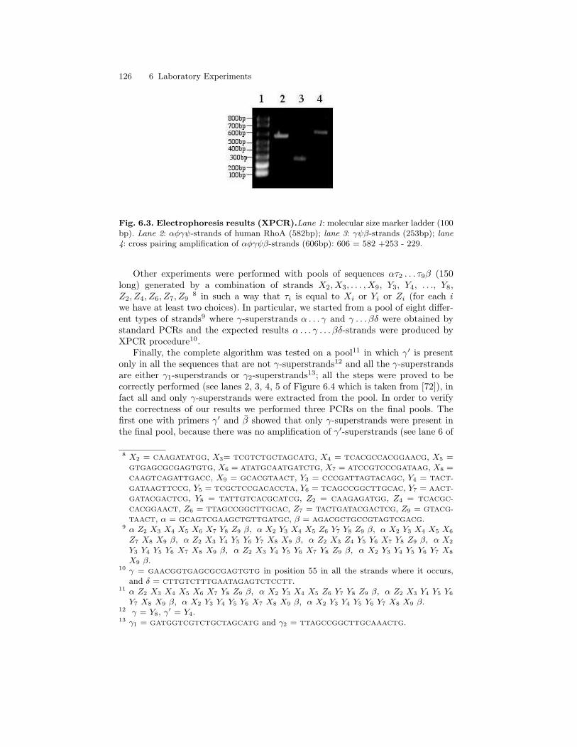
126 6 Laboratory Experiments
Fig. 6.3. Electrophoresis results (XPCR).Lane 1: molecular size marker ladder (100bp). Lane 2: αφγψ-strands of human RhoA (582bp); lane 3: γψβ-strands (253bp); lane4: cross pairing amplification of αφγψβ-strands (606bp): 606 = 582 +253 - 229.
Other experiments were performed with pools of sequences ατ2 . . . τ9β (150long) generated by a combination of strands X2, X3, . . . , X9, Y3, Y4, . . ., Y8,Z2, Z4, Z6, Z7, Z9
8 in such a way that τi is equal to Xi or Yi or Zi (for each iwe have at least two choices). In particular, we started from a pool of eight differ-ent types of strands9 where γ-superstrands α . . . γ and γ . . . βδ were obtained bystandard PCRs and the expected results α . . . γ . . . βδ-strands were produced byXPCR procedure10.
Finally, the complete algorithm was tested on a pool11 in which γ′ is presentonly in all the sequences that are not γ-superstrands12 and all the γ-superstrandsare either γ1-superstrands or γ2-superstrands13; all the steps were proved to becorrectly performed (see lanes 2, 3, 4, 5 of Figure 6.4 which is taken from [72]), infact all and only γ-superstrands were extracted from the pool. In order to verifythe correctness of our results we performed three PCRs on the final pools. Thefirst one with primers γ′ and β showed that only γ-superstrands were present inthe final pool, because there was no amplification of γ′-superstrands (see lane 6 of
8 X2 = CAAGATATGG, X3= TCGTCTGCTAGCATG, X4 = TCACGCCACGGAACG, X5 =GTGAGCGCGAGTGTG, X6 = ATATGCAATGATCTG, X7 = ATCCGTCCCGATAAG, X8 =CAAGTCAGATTGACC, X9 = GCACGTAACT, Y3 = CCCGATTAGTACAGC, Y4 = TACT-
GATAAGTTCCG, Y5 = TCGCTCCGACACCTA, Y6 = TCAGCCGGCTTGCAC, Y7 = AACT-
GATACGACTCG, Y8 = TATTGTCACGCATCG, Z2 = CAAGAGATGG, Z4 = TCACGC-
CACGGAACT, Z6 = TTAGCCGGCTTGCAC, Z7 = TACTGATACGACTCG, Z9 = GTACG-
TAACT, α = GCAGTCGAAGCTGTTGATGC, β = AGACGCTGCCGTAGTCGACG.9 α Z2 X3 X4 X5 X6 X7 Y8 Z9 β, α X2 Y3 X4 X5 Z6 Y7 Y8 Z9 β, α X2 Y3 X4 X5 X6
Z7 X8 X9 β, α Z2 X3 Y4 Y5 Y6 Y7 X8 X9 β, α Z2 X3 Z4 Y5 Y6 X7 Y8 Z9 β, α X2
Y3 Y4 Y5 Y6 X7 X8 X9 β, α Z2 X3 Y4 Y5 Y6 X7 Y8 Z9 β, α X2 Y3 Y4 Y5 Y6 Y7 X8
X9 β.10 γ = GAACGGTGAGCGCGAGTGTG in position 55 in all the strands where it occurs,
and δ = CTTGTCTTTGAATAGAGTCTCCTT.11 α Z2 X3 X4 X5 X6 X7 Y8 Z9 β, α X2 Y3 X4 X5 Z6 Y7 Y8 Z9 β, α Z2 X3 Y4 Y5 Y6
Y7 X8 X9 β, α X2 Y3 Y4 Y5 Y6 X7 X8 X9 β, α X2 Y3 Y4 Y5 Y6 Y7 X8 X9 β.12 γ = Y8, γ
′ = Y4.13 γ1 = GATGGTCGTCTGCTAGCATG and γ2 = TTAGCCGGCTTGCAAACTG.

6.4 XPCR-based generation 127
Fig. 6.4. Electrophoresis results (XPCR).Lane 1: molecular size marker ladder (25bp). Lane 2: amplification of α . . . γ strands (120 bp); lane 3: amplification of γ . . . βstrands (45 bp); lane 4: cross pairing amplification of α . . . γ and γ . . . β (150 bp). Lane5: positive control by PCR(γ, β), with γ at position -45; lane 6: negative control byPCR(γ′, β); lane 7, 8: positive controls by PCR(γ1, β) and PCR(γ2, β) respectively, withγ1 at position -125 and γ2 at position -75.
Figure 6.4). The last two PCRs with primers γ1, β, and γ2, β, respectively showedthat all the initial γ-superstrands were present in the final tube (see lanes 7 and 8of Figure 6.4).
6.4 XPCR-based generation
The following experiment showed that, given any SAT instance with 6 variables,the solution pool with sequences encoding all 64 assignments can be generated bystarting from 4 specific sequences and by using only XPCR and electrophoresis.The success of this experiment is meaningful because it can be scaled up easily toany number n of variables: starting from 4 specific sequences, all 2n combinationscan be generated by XPCR as proved by Proposition 4.1.
The experiment started on an initial pool having the four sequences 150bplong14
S1 = α Wa X1 X2 X3 X4 X5 X6 Za β
S2 = α Wb Y1 Y2 Y3 Y4 Y5 Y6 Zb β
S3 = α Wa X1 Y2 X3 Y4 X5 Y6 Zb β
14 S1 = GCAGTCGAAGCTGTTGATGC CAAGAGATGG TCGTCTGCTAGCATG TCACGC-
CACGGAACG GTGAGCGCGAGTGTG ATATGCAATGATCTG ATCCGTCCCGATAAG
CAAGTCAGATTGACC GCACGTAACT AGACGCTGCCGTAGTCGACG,S2 = GCAGTCGAAGCTGTTGATGC CAAGATATGG CCCGATTAGTACAGC TACT-
GATAAGTTCCG TCGCTCCGACACCTA TCAGCCGGCTTGCAC AACTGATACGACTCG
TATTGTCACGCATCG GTACGTAACT AGACGCTGCCGTAGTCGACG,S3 = GCAGTCGAAGCTGTTGATGC CAAGAGATGG TCGTCTGCTAGCATG TACT-
GATAAGTTCCG GTGAGCGCGAGTGTG TCAGCCGGCTTGCAC ATCCGTCCCGATAAG
TATTGTCACGCATCG GTACGTAACT AGACGCTGCCGTAGTCGACG,S4 = GCAGTCGAAGCTGTTGATGC CAAGATATGG CCCGATTAGTACAGC TCACGC-
CACGGAACG TCGCTCCGACACCTA ATATGCAATGATCTG AACTGATACGACTCG
CAAGTCAGATTGACC GCACGTAACT AGACGCTGCCGTAGTCGACG.
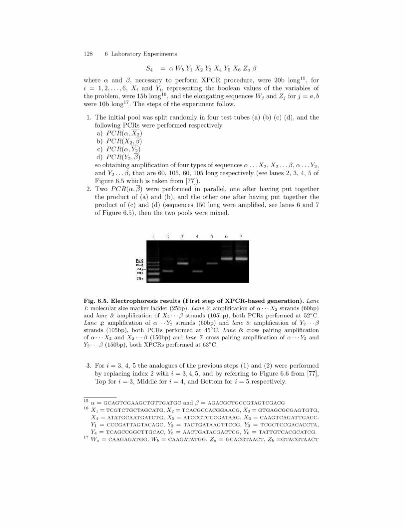
128 6 Laboratory Experiments
S4 = α Wb Y1 X2 Y3 X4 Y5 X6 Za β
where α and β, necessary to perform XPCR procedure, were 20b long15, fori = 1, 2, . . . , 6, Xi and Yi, representing the boolean values of the variables ofthe problem, were 15b long16, and the elongating sequences Wj and Zj for j = a, bwere 10b long17. The steps of the experiment follow.
1. The initial pool was split randomly in four test tubes (a) (b) (c) (d), and thefollowing PCRs were performed respectivelya) PCR(α,X2)b) PCR(X2, β)c) PCR(α, Y2)d) PCR(Y2, β)so obtaining amplification of four types of sequences α . . .X2, X2 . . . β, α . . . Y2,and Y2 . . . β, that are 60, 105, 60, 105 long respectively (see lanes 2, 3, 4, 5 ofFigure 6.5 which is taken from [77]).
2. Two PCR(α, β) were performed in parallel, one after having put togetherthe product of (a) and (b), and the other one after having put together theproduct of (c) and (d) (sequences 150 long were amplified, see lanes 6 and 7of Figure 6.5), then the two pools were mixed.
Fig. 6.5. Electrophoresis results (First step of XPCR-based generation). Lane1: molecular size marker ladder (25bp). Lane 2: amplification of α · · ·X2 strands (60bp)and lane 3: amplification of X2 · · ·β strands (105bp), both PCRs performed at 52◦C.Lane 4: amplification of α · · ·Y2 strands (60bp) and lane 5: amplification of Y2 · · ·βstrands (105bp), both PCRs performed at 45◦C. Lane 6: cross pairing amplificationof α · · ·X2 and X2 · · ·β (150bp) and lane 7: cross pairing amplification of α · · ·Y2 andY2 · · ·β (150bp), both XPCRs performed at 63◦C.
3. For i = 3, 4, 5 the analogues of the previous steps (1) and (2) were performedby replacing index 2 with i = 3, 4, 5, and by referring to Figure 6.6 from [77],Top for i = 3, Middle for i = 4, and Bottom for i = 5 respectively.
15 α = GCAGTCGAAGCTGTTGATGC and β = AGACGCTGCCGTAGTCGACG16 X1 = TCGTCTGCTAGCATG,X2 = TCACGCCACGGAACG,X3 = GTGAGCGCGAGTGTG,X4 = ATATGCAATGATCTG, X5 = ATCCGTCCCGATAAG, X6 = CAAGTCAGATTGACC.Y1 = CCCGATTAGTACAGC, Y2 = TACTGATAAGTTCCG, Y3 = TCGCTCCGACACCTA,Y4 = TCAGCCGGCTTGCAC, Y5 = AACTGATACGACTCG, Y6 = TATTGTCACGCATCG.
17 Wa = CAAGAGATGG, Wb = CAAGATATGG, Za = GCACGTAACT, Zb =GTACGTAACT

6.4 XPCR-based generation 129
4. An electrophoresis was performed to select the sequences 150 long amonglonger ones (generated by unspecific amplification).
Fig. 6.6. Electrophoresis results (Final steps of XPCR-based generation). Lane1: molecular size marker ladder (25bp). Top. Lane 2: amplification of α · · ·X3 strands(75bp), lane 3: amplification of X3 · · ·β strands (90bp), lane 4: amplification of α · · ·Y3
strands (75bp), lane 5: amplification of Y3 · · ·β strands (90bp), all PCRs performed at52◦C. Lane 6: cross pairing amplification of α · · ·X3 and X3 · · ·β (150bp) and lane 7:cross pairing amplification of α · · ·Y3 and Y3 · · ·β (150bp), both XPCRs performed at63◦C. Middle. Lane 2: amplification of α · · ·X4 strands (90bp), lane 3: amplification ofX4 · · ·β strands (75bp), lane 4: amplification of α · · ·Y4 strands (90bp), lane 5: ampli-fication of Y4 · · ·β strands (75bp), all PCRs performed at 42◦C. Lane 6: cross pairingamplification of α · · ·X4 and X4 · · ·β (150bp) and lane 7: cross pairing amplification ofα · · ·Y4 and Y4 · · ·β (150bp), both XPCRs performed at 63◦C. Bottom. Lane 2: am-plification of α · · ·X5 strands (105bp), lane 3: amplification of X5 · · ·β strands (60bp),lane 4: amplification of α · · ·Y5 strands (105bp), lane 5: amplification of Y5 · · ·β strands(60bp), all PCRs performed at 45◦C. Lane 6: cross pairing amplification of α · · ·X5 andX5 · · ·β (150bp) and lane 7: cross pairing amplification of α · · ·Y5 and Y5 · · ·β (150bp),both XPCRs performed at 63◦C.

130 6 Laboratory Experiments
By the electrophoresis results one can note that the sequences 150 long presentin the pool were amplified (in linear or exponential manner) during each step.Although this phenomenon did not disturb the correctness of the ‘computation’,it caused noise and useless occupation of space in a test tube by increasing theunspecific matter, as one can see clearly in Figure 6.6. An improved experimentcould be performed very easily by inserting intermediate electrophoresis steps toclean the signal from the noise caused by these amplifications. For example, elec-trophoresis separations after the cutting steps of each XPCR, could eliminate thestrands 150 long, for decreasing the production of unspecific matter.
6.4.1 Recombination witnesses
The success of the experiment was tested in a first stage by the presence of all the(four) recombination witnesses (see Proposition 4.8), that has been guaranteed bythe amplification of the following PCRs on the final pool (see lanes 2, 3, 4, 5 ofFigure 6.7).
1. PCR(X1X2Y3, Y4X5X6)2. PCR(Y1Y2X3, X4Y5Y6)3. PCR(Y1X2X3, Y4Y5X6)4. PCR(X1Y2Y3, X4X5Y6)
These PCRs were performed with primers 45 long, that are very specific butvery long with respect to primers of a standard PCR (see Section 6.2.1). In thiscase the melting temperature had to be lower than usual, thus one could suspectthat only proper substrings of these primers were annealed with the sequencespresent in the pool and that amplifications above could have been generated bysequences different from W1 = X1X2Y3Y4X5X6, W2 = Y1Y2X3X4Y5Y6, T1 =Y1X2X3Y4Y5X6 and T2 = X1Y2Y3X4X5Y6 (respectively). In order to verify thatit was not the case, two negative controls were performed by PCRs with primers45 long whose only one should not be present in the pool. This primer was asubsequence of βMyc and was extracted from the human gene RhoA.
1. PCR(α, βMyc)2. PCR(X1X2Y3, βMyc)
In both these last PCRs no amplification was obtained, as expected (see lanes6 and 7 of Figure 6.7). However, such proof was not definitively convincing andmore checks seemed necessary.
In the meantime Theorem 4.9 came up, thus checking the presence of just acouple of recombination witnesses in the final pool became enough for the successof the experiment. Thereafter, the presence of W1 and W2 in the final pool wasguaranteed by the amplification of the following PCRs18.
For each sequence the presence of two extremal pieces 1,6 is checked by PCR,then, on the amplification product of this PCR, the presence of pieces 2,4 is18 Thanks to an anonymous referee of the 11th International Meeting on DNA Com-
puting, June 6-9 2005, London, Ontario, for his/her interesting comments and forsuggesting us to find a better procedure checking the complete recombination of thefinal pool.
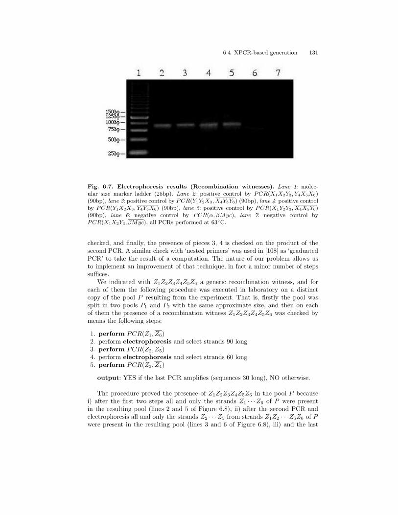
6.4 XPCR-based generation 131
Fig. 6.7. Electrophoresis results (Recombination witnesses). Lane 1: molec-ular size marker ladder (25bp). Lane 2: positive control by PCR(X1X2Y3, Y4X5X6)(90bp), lane 3: positive control by PCR(Y1Y2X3, X4Y5Y6) (90bp), lane 4: positive controlby PCR(Y1X2X3, Y4Y5X6) (90bp), lane 5: positive control by PCR(X1Y2Y3, X4X5Y6)(90bp), lane 6: negative control by PCR(α, βMyc), lane 7: negative control byPCR(X1X2Y3, βMyc), all PCRs performed at 63◦C.
checked, and finally, the presence of pieces 3, 4 is checked on the product of thesecond PCR. A similar check with ‘nested primers’ was used in [108] as ‘graduatedPCR’ to take the result of a computation. The nature of our problem allows usto implement an improvement of that technique, in fact a minor number of stepssuffices.
We indicated with Z1Z2Z3Z4Z5Z6 a generic recombination witness, and foreach of them the following procedure was executed in laboratory on a distinctcopy of the pool P resulting from the experiment. That is, firstly the pool wassplit in two pools P1 and P2 with the same approximate size, and then on eachof them the presence of a recombination witness Z1Z2Z3Z4Z5Z6 was checked bymeans the following steps:
1. perform PCR(Z1, Z6)2. perform electrophoresis and select strands 90 long3. perform PCR(Z2, Z5)4. perform electrophoresis and select strands 60 long5. perform PCR(Z3, Z4)
output: YES if the last PCR amplifies (sequences 30 long), NO otherwise.
The procedure proved the presence of Z1Z2Z3Z4Z5Z6 in the pool P becausei) after the first two steps all and only the strands Z1 · · ·Z6 of P were presentin the resulting pool (lines 2 and 5 of Figure 6.8), ii) after the second PCR andelectrophoresis all and only the strands Z2 · · ·Z5 from strands Z1Z2 · · ·Z5Z6 of Pwere present in the resulting pool (lines 3 and 6 of Figure 6.8), iii) and the last
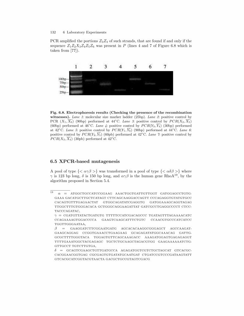
132 6 Laboratory Experiments
PCR amplified the portions Z3Z4 of such strands, that are found if and only if thesequence Z1Z2X3Z4Z5Z6 was present in P (lines 4 and 7 of Figure 6.8 which istaken from [77]).
Fig. 6.8. Electrophoresis results (Checking the presence of the recombinationwitnesses). Lane 1: molecular size marker ladder (25bp). Lane 2: positive control byPCR (X1, X6) (90bp) performed at 44◦C. Lane 3: positive control by PCR(X2, X5)(60bp) performed at 46◦C. Lane 4: positive control by PCR(Y3, Y4) (30bp) performedat 42◦C. Lane 5: positive control by PCR(Y1, Y6) (90bp) performed at 44◦C. Lane 6:positive control by PCR(Y2, Y5) (60pb) performed at 42◦C. Lane 7: positive control byPCR(X3, X4) (30pb) performed at 42◦C.
6.5 XPCR-based mutagenesis
A pool of type {< αγβ >} was transformed in a pool of type {< αδβ >} whereγ is 123 bp long, δ is 150 bp long, and αγβ is the human gene RhoA19, by thealgorithm proposed in Section 5.4.
19 α = ATGGCTGCCATCCGGAAG AAACTGGTGATTGTTGGT GATGGAGCCTGTG-
GAAA GACATGCTTGCTCATAGT CTTCAGCAAGGACCAGTT CCCAGAGGTGTATGTGCC
CACAGTGTTTGAGAACTAT GTGGCAGATATCGAGGTG GATGGAAAGCAGGTAGAG
TTGGCTTTGTGGGACACA GCTGGGCAGGAAGATTAT GATCGCCTGAGGCCCCT CTCC-
TACCCAGATAC,γ = CGATGTTATACTGATGTG TTTTTCCATCGACAGCCC TGATAGTTTAGAAAACATC
CCAGAAAAGTGGACCCCA GAAGTCAAGCATTTCTGTC CCAACGTGCCCATCATCC
TGGTTGGGAATAA,β = GAAGGATCTTCGGAATGATG AGCACACAAGGCGGGAGCT AGCCAAGAT-
GAAGCAGGAG CCGGTGAAACCTGAAGAAG GCAGAGATATGGCAAACAG GATTG-
GCGCTTTTGGGTACA TGGAGTGTTCAGCAAAGACC AAAGATGGAGTGAGAGAGGT
TTTTGAAATGGCTACGAGAGC TGCTCTGCAAGCTAGACGTGG GAAGAAAAAATCTG-
GTTGCCT TGTCTTGTGA,δ = GCAGTCGAAGCTGTTGATGCCA AGAGATGGTCGTCTGCTAGCAT GTCACGC-
CACGGAACGGTGAG CGCGAGTGTGATATGCAATGAT CTGATCCGTCCCGATAAGTATT
GTCACGCATCGGTACGTAACTA GACGCTGCCGTAGTCGACG
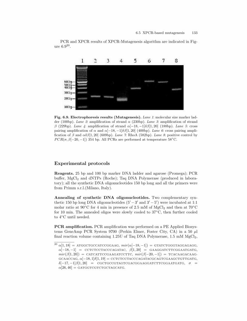
6.5 XPCR-based mutagenesis 133
PCR and XPCR results of XPCR-Mutagenesis algorithm are indicated in Fig-ure 6.920.
Fig. 6.9. Electrophoresis results (Mutagenesis). Lane 1: molecular size marker lad-der (100bp). Lane 2: amplification of strand α (230bp). Lane 3: amplification of strandβ (229bp). Lane 4: amplification of strand α[−18,−1]δβ[1, 20] (188bp). Lane 5: crosspairing amplification of α and α[−18,−1]δβ[1, 20] (400bp). Lane 6: cross pairing ampli-fication of β and αδβ[1, 20] (609bp). Lane 7: RhoA (582bp). Lane 8: positive control byPCR(σ, β[−20,−1]) 354 bp. All PCRs are performed at temperature 58◦C.
Experimental protocols
Reagents. 25 bp and 100 bp marker DNA ladder and agarose (Promega); PCRbuffer, MgCl2 and dNTPs (Roche); Taq DNA Polymerase (produced in labora-tory); all the synthetic DNA oligonucleotides 150 bp long and all the primers werefrom Primm s.r.l.(Milano, Italy).
Annealing of synthetic DNA oligonucleotides. Two complementary syn-thetic 150 bp long DNA oligonucleotides (5′−3′ and 3′−5′) were incubated at 1:1molar ratio at 90◦C for 4 min in presence of 2.5 mM of MgCl2 and then at 70◦Cfor 10 min. The annealed oligos were slowly cooled to 37◦C, then further cooledto 4◦C until needed.
PCR amplification. PCR amplification was performed on a PE Applied Biosys-tems GeneAmp PCR System 9700 (Perkin Elmer, Foster City, CA) in a 50 µlfinal reaction volume containing 1.25U of Taq DNA Polymerase, 1.5 mM MgCl2,
20 α[1, 18] = ATGGCTGCCATCCGGAAG, mir(α[−18,−1]) = GTATCTGGGTAGGAGAGG,α[−18,−1] = CCTCTCCTACCCAGATAC, β[1, 20] = GAAGGATCTTCGGAATGATG,mir(β[1, 20]) = CATCATTCCGAAGATCCTTC, mir(β[−20,−1]) = TCACAAGACAAG-
GCAACCAG, α[−18, 1]δ[1, 19] = CCTCTCCTACCCAGATACGCAGTCGAAGCTGTTGATG,δ[−17,−1]β[1, 20] = CGCTGCCGTAGTCGACGGAAGGATCTTCGGAATGATG, σ =α[26, 46] = GATGGTCGTCTGCTAGCATG.

134 6 Laboratory Experiments
200 µM each dNTP, PCR buffer, 80 ng DNA template, 0.5-1 µM of forward andreverse primers. The reaction mixture was preheated to 95◦C for 5 min. (initialdenaturing), termocycled 30 times: 95◦C for 30 sec (denaturing), different tem-peratures (see figures) for 30 sec. (annealing), 72◦C for 15 sec. (elongation); finalextensions was performed at 72◦C for 5/10 min.
Preparation and running of gels. Gels were prepared in 7 × 7 cm plastic gelcassettes with appropriate combs for well formation. Approximately 20 ml of 4%agarose solutions were poured into the cassettes and allowed to polymerize for10 min. Agarose gels were put in the electrophoresis chamber and electrophoresiswas carried out at 10 volt/cm2, then the bands of the gels are detected by a gelscanner. The DNA bands (final PCR products) of interest were excised from thegel and the DNA was purified from the gel slices by Promega Kit (Wizard SV Geland PCR Clean-Up System).
The experiments reported in this chapter may be found in the following articles.
• G. F., C. Giagulli, C. Laudanna, V. Manca, DNA Extraction by Cross PairingPCR, C. Ferretti G. Mauri C. Zandron eds, Preliminary Proceedings of 10thInternational Meeting on DNA Computing: DNA 10, pp 193-201, Universityof Milano Bicocca, Milan, Italy, June 7-10 2004.
• G. F., C. Giagulli, C. Laudanna, V. Manca, DNA Extraction by XPCR, C.Ferretti G. Mauri C. Zandron eds, 10th International Workshop on DNA Com-puting, DNA 10, Milan, Italy, June 2004, Revised Selected Papers, LNCS 3384,Springer, pp 104-112, 2005.
• G. F., V. Manca, C. Giagulli, C. Laudanna, DNA Recombination by XPCR,Revised Selected Paper in A. Carbone, N.A. Pierce Eds: DNA11, June 6-92005, London, Ontario, Canada, LNCS 3892, pp 55-66, 2006.

7
A Model for DNA Self-Assembly
It is not knowledge, but the act of learning,not possession, but the act of getting there,
which grants the greatest enjoyment.
Carl Friedrich Gauss1
The process in which substructures, driven by their selective affinity, are spon-taneously self-ordered into superstructures, is now widely referred to as self-assembly. DNA can shape itself into many forms to achieve its purpose in life. Thecrystal structure of the junction between two of its forms provides insight into howDNA might accomplish some of these acrobatics [220]. Algorithms and informa-tion, fundamental to technological and biological organization, are also an essentialaspect of DNA self-assembly [199]. The construction of molecular scale structuresis one of the challenge at the core of an emerging discipline of Nanoscience, whichis at a critical stage of development. The powerful molecular recognition systememployed in DNA base pairing is used for constructing experimentally the self-assembly of three dimensional DNA structures (see Figure 7.1 comprising of DNAcube taken from [41] and DNA octahedron taken from [246]).
In nature, DNA appears as linear double stranded molecule (in eukaryotes)or in a circular form (mostly in viruses and bacteria, prokaryotes). Circular DNAmolecules can be obtained also in a laboratory by joining (ligating) the ends of alinear DNA. They have been used in several models of DNA based computers andas building blocks for DNA knots [111]. If one imagines of unravelling the familiarhelix (that is named B-DNA) and then twisting it up the other way around, thenthe result (that is named Z-DNA) is not so visually appealing, and not so stable,but it has some intriguing biology [220]. Left-handed Z-DNA exists in nature asa higher-energy and inherently unstable form of the double helix. In theory, anyknot can be constructed in laboratory by using right-handed B-DNA for negativecrossings and left-handed Z-DNA for positive crossings [111]. The Borromean ringsdisplayed in Figure 1.1 were assembled by using B and Z DNA [157].
1 Letter to Bolyai, 1808.
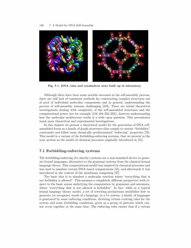
136 7 A Model for DNA Self-Assembly
Fig. 7.1. DNA cube and octahedron were built up in laboratory.
Although there have been some notable successes in the self-assembly process,there are still lack of consistent methods for constructing complex structures outof pool of individual molecular components and in general, understanding theprocess of self-assembly remains challenging [218]. There are initial theoreticalinvestigations dealing with complexity of the self-assembled structures and thecomputational power (see for example [116,194,222,235]), however understandinghow the molecular architecture works is a wide open question. This necessitatesmuch more theoretical and experimental investigations.
In this chapter we present a theoretical model for the generation of DNA self-assembled forms as a family of graph structures that comply to certain “forbidden”constraints and follow some chemically predetermined “enforcing” properties [73].This model is a variant of the forbidding-enforcing systems, that we present in thenext section as the model of chemical processes originally introduced in [55].
7.1 Forbidding-enforcing systems
The forbidding-enforcing (f-e shortly) systems are a non-standard device to gener-ate formal languages, alternative to the grammar systems from the classical formallanguage theory. This computational model was inspired by chemical processes andwas used to simulate certain DNA based computations [55], and afterwards it wasintroduced in the context of the membrane computing [37].
The basic idea is to simulate a molecular reaction where “everything that isnot forbidden is allowed”. This assumes a completely different perspective with re-spect to the basic axiom underlying the computation by grammars and automata,where “everything that is not allowed is forbidden”. In fact, while in a typicalformal language theory model, a set of rewriting productions establishes how togenerate (or recognize) words of a language, in a f-e system, a family of languagesis generated by some enforcing conditions, dictating certain evolving rules for thesystem and some forbidding conditions, given as a group of patterns which can-not occur together at the same time. The enforcing rules ensure that if a certain
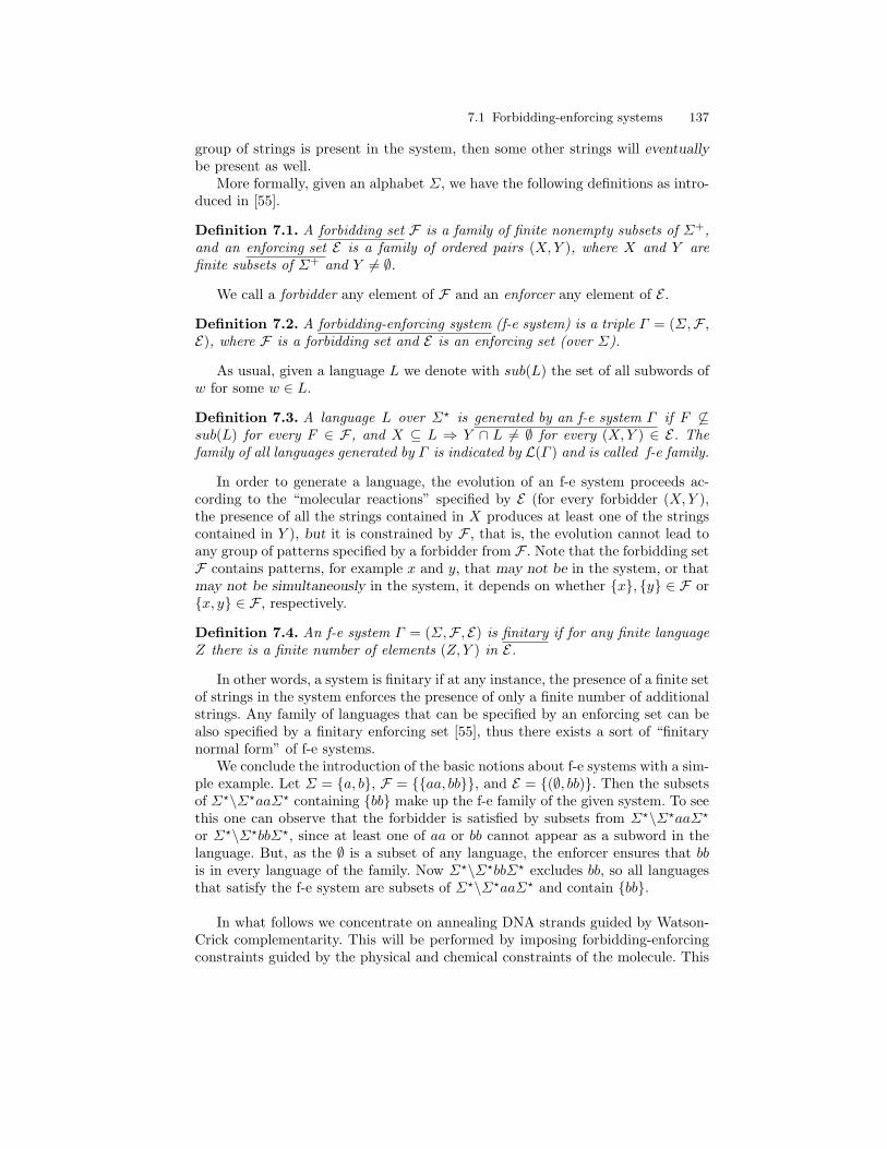
7.1 Forbidding-enforcing systems 137
group of strings is present in the system, then some other strings will eventuallybe present as well.
More formally, given an alphabet Σ, we have the following definitions as intro-duced in [55].
Definition 7.1. A forbidding set F is a family of finite nonempty subsets of Σ+,and an enforcing set E is a family of ordered pairs (X,Y ), where X and Y arefinite subsets of Σ+ and Y 6= ∅.
We call a forbidder any element of F and an enforcer any element of E .
Definition 7.2. A forbidding-enforcing system (f-e system) is a triple Γ = (Σ,F ,E), where F is a forbidding set and E is an enforcing set (over Σ).
As usual, given a language L we denote with sub(L) the set of all subwords ofw for some w ∈ L.
Definition 7.3. A language L over Σ? is generated by an f-e system Γ if F 6⊆sub(L) for every F ∈ F , and X ⊆ L ⇒ Y ∩ L 6= ∅ for every (X,Y ) ∈ E. Thefamily of all languages generated by Γ is indicated by L(Γ ) and is called f-e family.
In order to generate a language, the evolution of an f-e system proceeds ac-cording to the “molecular reactions” specified by E (for every forbidder (X,Y ),the presence of all the strings contained in X produces at least one of the stringscontained in Y ), but it is constrained by F , that is, the evolution cannot lead toany group of patterns specified by a forbidder from F . Note that the forbidding setF contains patterns, for example x and y, that may not be in the system, or thatmay not be simultaneously in the system, it depends on whether {x}, {y} ∈ F or{x, y} ∈ F , respectively.
Definition 7.4. An f-e system Γ = (Σ,F , E) is finitary if for any finite languageZ there is a finite number of elements (Z, Y ) in E.
In other words, a system is finitary if at any instance, the presence of a finite setof strings in the system enforces the presence of only a finite number of additionalstrings. Any family of languages that can be specified by an enforcing set can bealso specified by a finitary enforcing set [55], thus there exists a sort of “finitarynormal form” of f-e systems.
We conclude the introduction of the basic notions about f-e systems with a sim-ple example. Let Σ = {a, b}, F = {{aa, bb}}, and E = {(∅, bb)}. Then the subsetsof Σ?\Σ?aaΣ? containing {bb} make up the f-e family of the given system. To seethis one can observe that the forbidder is satisfied by subsets from Σ?\Σ?aaΣ?
or Σ?\Σ?bbΣ?, since at least one of aa or bb cannot appear as a subword in thelanguage. But, as the ∅ is a subset of any language, the enforcer ensures that bbis in every language of the family. Now Σ?\Σ?bbΣ? excludes bb, so all languagesthat satisfy the f-e system are subsets of Σ?\Σ?aaΣ? and contain {bb}.
In what follows we concentrate on annealing DNA strands guided by Watson-Crick complementarity. This will be performed by imposing forbidding-enforcingconstraints guided by the physical and chemical constraints of the molecule. This
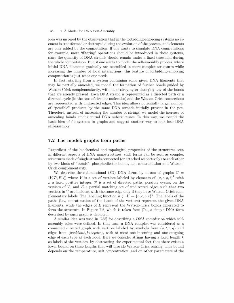
138 7 A Model for DNA Self-Assembly
idea was inspired by the observation that in the forbidding-enforcing systems no el-ement is transformed or destroyed during the evolution of the process, and elementsare only added by the computation. If one wants to simulate DNA computationsfor example, more ‘filtering’ operations should be introduced in these systems,since the quantity of DNA strands should remain under a fixed threshold duringthe whole computation. But, if one wants to model the self-assembly process, whereinitial DNA filaments gradually are assembled in more complex structures whileincreasing the number of local interactions, this feature of forbidding-enforcingcomputation is just what one needs.
In fact, starting from a system containing some given DNA filaments thatmay be partially annealed, we model the formation of further bonds guided byWatson-Crick complementarity, without destroying or changing any of the bondsthat are already present. Each DNA strand is represented as a directed path or adirected cycle (in the case of circular molecules) and the Watson-Crick connectionsare represented with undirected edges. This idea allows potentially larger numberof “possible” products by the same DNA strands initially present in the pot.Therefore, instead of increasing the number of strings, we model the increase ofannealing bonds among initial DNA substructures. In this way, we extend thebasic idea of f-e systems to graphs and suggest another way to look into DNAself-assembly.
7.2 The model: graphs from paths
Regardless of the biochemical and topological properties of the structures seenin different aspects of DNA nanostructures, such forms can be seen as complexstructures made of single strands connected (or attached respectively) to each otherby two kinds of “bonds”: phosphodiester bonds, i.e., concatenation and Watson-Crick complementarity.
We describe three-dimensional (3D) DNA forms by means of graphs G =(V,P, E, ξ) where V is a set of vertices labeled by elements of {a, c, g, t}k withk a fixed positive integer, P is a set of directed paths, possibly cycles, on thevertices of V , and E a partial matching set of undirected edges such that twovertices in V are incident with the same edge only if they have Watson-Crick com-plementary labels. The labelling function is ξ : V → {a, c, g, t}k. The labels of thepaths (i.e., concatenation of the labels of the vertices) represent the given DNAfilaments, while the edges of E represent the Watson-Crick bonds generated toform the structure. In Figure 7.2, which is taken from [74], a simple DNA formdescribed by such graph is depicted.
A similar idea was used in [235] for describing a DNA complex on which self-assembly rules were defined. In that case, a DNA complex was considered as aconnected directed graph with vertices labeled by symbols from {a, t, c, g} andedges from {backbone, basepair}, with at most one incoming and one outgoingedge of each type at each node. Here we consider strings having a fixed length kas labels of the vertices, by abstracting the experimental fact that there exists alower bound on these lengths that will provide Watson-Crick pairing. This bounddepends on the temperature, salt concentration, and on other parameters of the

7.2 The model: graphs from paths 139
β
δ δ
φφ
φ
β
γ
γ η
η
1 2
β 3
β
β 1
2
45 1
2
3
1
21
2
β β
β
β
βφ
φ
φγ
γ
η
η
54
3
2 21
2
2
3
1
1
1
δ 2δ 1
Fig. 7.2. Example of a self-assembled structure. One may note that: δ1 = β4,δ2 = φ1, β3 = φ2, η1 = φ3, γ2 = β2 and η2 = γ1.
experiment. It is quite intuitive that starting from the same filaments the numberof possible self-assembled DNA forms increases as the k value decreases, which inour case represents the (minimum) length of the attached portions. Here we focuson the graph structures corresponding to self-assembled forms, by fixing the valuefor k (for example, k = 5, which is approximatively the length of a half helicalturn) and the complementarity between two strings of length k.
Another possibility that can appear experimentally but is ignored in this expo-sition is the overlapping of strings. Consider the ten symbol string w = actactacta.For k = 5, we can write w = uv with u = actac and v = tacta. However thereare two occurrences of u as a substring of w, i.e., w = act · u · ta. In practice, acomplementary string to u can anneal to both of these occurrences. Our modelassumes that none of the strings representing DNA strands have such labelling.
On the other hand, we suppose that the correspondence from vertices to (la-belling) strings may not necessarily be injective, in fact more than one occurrenceof a string may be located along the filaments forming the structure. Thereforewe consider a labelling function ξ : V → {a, c, g, t}k that assigns a string from{a, t, c, g}k to each vertex from V . Further, in order to keep the model more real-istic, all our graphs are finite graphs, where V and P are (given) finite sets.
The description of a self-assembly structure by means of such a graph simplifiesthe representation and emphasizes the interrelations between the substructures,for example a loop (a cycle with only one undirected edge) corresponds to a hairpinformation [209], and a connected component of the graph corresponds to one DNAstructure.
Consider the triple cross over molecule TX [136] designed in the Ned Seeman’slaboratory (see Figure 7.3 top). This complex structure is made of six strands,although there are examples of similar TX molecules with fewer strands. It canbe presented as a graph in the following way. The length of the molecule is about4.5 helical turns which corresponds to roughly 48 bases. For this, we consider36 vertices, each labeled with a string of length 8. In Figure 7.3, which is takenfrom [73], (a) the TX molecule is simplified by ignoring the helical turns and theWatson-Crick pairing corresponding to 8 consecutive nucleotides is identified with

140 7 A Model for DNA Self-Assembly
a group of five short bars. In Figure 7.3 (b) - (d) the process of obtaining a graphstructure corresponding to the TX molecule is presented. The directed edges followthe 5′ - 3′ direction of the strand, and the undirected edges indicate the sequenceof 8 base pairs.
Fig. 7.3. Triple cross over molecule (TX) as a self-assembly graph.
If size is ignored, theoretically, from a few types of initial pieces, any shapecan be self-assembled by spontaneous local bonding. In fact, the Kolmogorov com-plexity of a shape provides upper and lower bounds for the number of tile typesnecessary to self-assemble a given shape (at some scale) [222]. Nevertheless, to findstrands that generate given structures remains a difficult design problem.
One can consider the converse question, what kind of forms are obtained byadding in a pot some given DNA substructures (or filaments). In other terms,assume a labeled graph structure (V,P, ξ, E) where V is the set of vertices, Pthe set of paths, ξ the labelling function, and E a given partial matching on thevertices. What are the edges that can be added in the (possibly empty) matchingset E such that there exists a DNA structure corresponding to the obtained graph?It is clear that there exist graphs (V,P, ξ, E) that do not represent DNA structures,for example, they do not take in account some physical constraints. Figure 7.4,which is taken from [73], shows an example of two such structures.
Thus, given a collection of directed paths and cycles with vertices labeled bystrings, we are going to consider (in Subsection 7.3.1) a set of valid graphs, where“forbidden” structures are not present. In particular, in order to obtain a graph

7.3 Forbidding-enforcing graphs 141
Fig. 7.4. Examples of graphs that do not correspond to a DNA structure.
which represents a self-assembled DNA structure, the matching set must respectcertain constraints defined by means of a set of forbidden subgraphs which onthe other hand follow physical and chemical restrictions of the DNA molecule.Such restrictions about the interrelations between DNA strings can be formulatedonly locally [119]. Moreover, a set of enforcing structures is considered in orderto describe the parallelism intrinsic to the nature of self-assembly. This includesthe considerations that further pairing of partially annealed molecules is preferredover strands that are far apart.
Molecular self-assembly is an inherently parallel process which begins anywhereit is energetically favored. Here we assume all thermodynamical conditions nec-essary for self-assembly are present such that assembly is obtained wherever it isstructurally possible. Another assumption coming from the chemical structure ofDNA is its inflexibility. For example, for a given k the model forbids formation ofdouble stranded DNA circular molecules with length less than nk nucleotides. Wecan namely assume that nk ≥ 100, in which case n would depend on our choice ofk.
Let us consider in the next section the theoretical model for forbidding-enforcing systems on graphs [73].
7.3 Forbidding-enforcing graphs
Consider graphs of the type G = (V,P, E), where V is a finite set of vertices, P isa set of oriented paths, possibly cycles, on vertices of V , and E is partial matching,that is, a set of undirected edges such that any vertex of V is incident to at mostone other vertex. We denote this family of graphs with G. If p ∈ P we indicatewith A(p) the set of arcs included in the path p, and call A(P) the set ∪p∈PA(p).
Definition 7.5. Given a positive integer m a m-local g-forbidder is a graph(V,P, E) in G with |A(p)| < m for every p ∈ P. A g-enforcer is an ordered pair(X,Y ), where X = (V,P, E) ∈ G and Y = (V ′,P ′, E′) ∈ G are such that V = V ′,P = P ′ and E ( E′.
The constant m is included to ensure that all forbidders act locally, i.e., oneonly needs to concentrate on paths with not more than m vertices. This in generalmay depend on the experimental conditions. In what follows, we assume that mis fixed and all m-local g-forbidders are referred to simply as g-forbidders.
The set F of g-forbidders is called forbidding set, and the set E of g-enforcersis called the enforcing set of a family of graphs.
As in the original definition, a forbidding set may be infinite and the onlyrequirement is that each forbidder is finite [55]. A g-forbidder is finite if it has a

142 7 A Model for DNA Self-Assembly
finite number of arcs and edges. Moreover, regardless of the presence of the otherforbidders, each g-forbidder cannot appear as subgraph of a graph satisfying thatforbidder.
Definition 7.6. A g-f-e system is a structure Γ = (V,P, E,F , E), where V is afinite set of vertices, P is a set of directed paths, possibly cycles, on vertices ofV , E is a partial matching on V , F is a set of g-forbidders and E is a set ofg-enforcers.
Given a graph G = (V,P, E) ∈ G, we call sub(G) the set of all subgraphs(V0,P0, E0) of G, where V0 ⊆ V , every p0 ∈ P0 is a path on vertices from V0 suchthat p0 ⊆ p for some p ∈ P and E0 ⊆ E is a matching set on V0. We write G′ ≤ Gfor G′ ∈ sub(G). Similarly, G′ < G if G′ ≤ G but G′ 6= G.
Definition 7.7. A graph G = (V,P, E?) is generated by the g-f-e system Γ =(V,P, E,F , E) if, E ⊂ E?, F 6∈ sub(G) for every F ∈ F , and for every (X,Y ) ∈ E,if X ∈ sub(G) then there is Y ′ ∈ sub(G) such that X < Y ′ ≤ Y .
The family of all graphs generated by a graph-forbidding-enforcing system Γis indicated by G(Γ ). The elements of G(Γ ) are called assembled graphs.
Similarly as in the original definition of forbidding-enforcing systems, the evo-lution of a g-f-e system proceeds according to the molecular reactions specifiedthrough E by increasing the elements of the matching set E, but not allowingsubgraphs that are forbidden by F .
7.3.1 Graphs for DNA structures
Now we concentrate on the model of g-f-e systems that simulate the self-assemblyprocess of DNA. In this case the vertices of the graphs are labeled by strings fromalphabet {a, g, c, t}k. Hence, all graphs belong to the class of graphs (V,P, E, ξ)where V , P, and E are the same as in the previous section, and ξ : V → {a, g, c, t}kis the labelling of the vertices. All definitions for g-forbidders, g-enforcers and g-f-esystems are transfered to this class of graphs in a straight forward way. We notethat the labelling of the vertices of every subgraph of a graph is preserved.
Consider a g-f-e system G(Γ ) with Γ = (V,P, E, ξ,F , E) where the DNA stringsare associated to the paths P are given by the (finite number of) initial DNAfilaments in the pot, the set E is given by the Watson-Crick bonds present inthe initial DNA substructures. We specify a set of forbidders and enforcers thatensures construction of DNA structures.
The forbidding set F forbids constructions that are “impossible” by the phys-ical and chemical properties of DNA. We list three g-forbidders that are moststraightforward observations and should be included in every g-f-e system thatsimulates DNA self-assembly.
1. proper annealing (a pair of vertices is matched only if they have complementarylabels)
F0 = (V = {v1, v2},P = ∅, E = {e = {v1, v2}} , ξ(v1) = α, ξ(v2) 6= α)
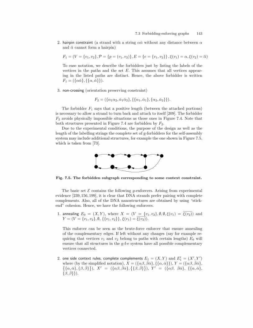
7.3 Forbidding-enforcing graphs 143
2. hairpin constraint (a strand with a string αα without any distance between αand α cannot form a hairpin)
F1 = (V = {v1, v2},P = {p = (v1, v2)}, E = {e = {v1, v2}} , ξ(v1) = α, ξ(v2) = α)
To ease notation, we describe the forbidders just by listing the labels of thevertices in the paths and the set E. This assumes that all vertices appear-ing in the listed paths are distinct. Hence, the above forbidder is writtenF1 = ({αα}, {{α, α}}).
3. non-crossing (orientation preserving constraint)
F2 = ({α1α2, α1α2}, {{α1, α1}, {α2, α2}}).
The forbidder F1 says that a positive length (between the attached portions)is necessary to allow a strand to turn back and attach to itself [209]. The forbidderF2 avoids physically impossible situations as those ones in Figure 7.4. Note thatboth structures presented in Figure 7.4 are forbidden by F2.
Due to the experimental conditions, the purpose of the design as well as thelength of the labelling strings the complete set of g-forbidders for the self-assemblysystem may include additional structures, for example the one shown in Figure 7.5,which is taken from [73].
Fig. 7.5. The forbidden subgraph corresponding to some context constraint.
The basic set E contains the following g-enforcers. Arising from experimentalevidence [239,156,199], it is clear that DNA strands prefer pairing with completecomplements. Also, all of the DNA nanostructures are obtained by using “stick-end” cohesion. Hence, we have the following enforcers.
1. annealing E0 = (X,Y ), where X = (V = {v1, v2}, ∅, ∅, ξ(v1) = ξ(v2)) andY = (V = {v1, v2}, ∅, {{v1, v2}}, ξ(v1) = ξ(v2)).
This enforcer can be seen as the brute-force enforcer that ensure annealingof the complementary edges. If left without any changes (say for example re-quiring that vertices v1 and v2 belong to paths with certain lengths) E0 willensure that all structures in the g-f-e system have all possible complementaryvertices connected.
2. one side context rules, complete complements E1 = (X,Y ) and E′1 = (X ′, Y ′)
where (by the simplified notation), X = ({αβ, βα}, {{α, α}}), Y = ({αβ, βα},{{α, α}, {β, β}
}), X ′ = ({αβ, βα},
{{β, β}
}), Y ′ = ({αβ, βα}, {{α, α},
{β, β}}).

144 7 A Model for DNA Self-Assembly
E′1 is essentially the same as E1 except that the initial hybridization has oc-
curred at the other side of the molecule (one can see the two possibilities inFigure 7.6, which is taken from [74]). The enforcers E1 and E′
1 ensure that fullcomplements of the strands are preferred.
α α
α
α α
α
β β
β
β
β
Fig. 7.6. One side context enforcing rule allowed by E1 and E′1.
3. sticky end cohesion (see Figure 7.7 (a))E2 = (X,Y ) where (by the simplified notation)X = ({αβ, γβ}, {{α, α}, {γ, γ}})Y = ({αβ, γβ},
{{α, α}, {γ, γ}, {β, β}
})
4. joining (see Figure 7.7 (b))E3 = (X,Y ) where (by the simplified notation)X = ({αβγδ, δγ, βα}, ∅)Y = ({αβγδ, δγ, βα},
{{α, α}, {β, β}, {γ, γ}, {δ, δ
})
The enforcers that ensure sticky end cohesion are depicted in Figure 7.7, whichwas drawn by Natasa Jonoska (Mathematics Deptartment, USF, USA) for [73].The left side of the figure is the partial annealing of the molecules and the rightside depicts the graphs corresponding to these two cases. Note that the enforcerE3 adds one, two, three or four new undirected edges. If only one edge is added,there is no guarantee that the full annealing will happen, but by the enforcers E1
and E′1 there will be at least one more edge added.
As an example of enforced graphs we indicate the formation of the structuredjunctions as depicted in the Figure 7.8, which is taken from [74], where one can seesome interactions between three, four, five and six initial paths. These formationsare not present in nature, but they were all made in laboratory by self-assembly.
The sticky-end attachment simulated by the enforcer E2 is basic for the for-mation of self-assembled structures (see Figure 7.8). The well known n-armedbranched molecules, here enforced by E3, were used to assembly polyhedrons,quadrilateral, the cube and the truncated octahedron in Figure 7.1 and seem par-ticularly suitable for DNA graph constructions [118]. Figure 7.8 is quite abstract,in reality the angles between the “arms” are known to be flexible, at least if we
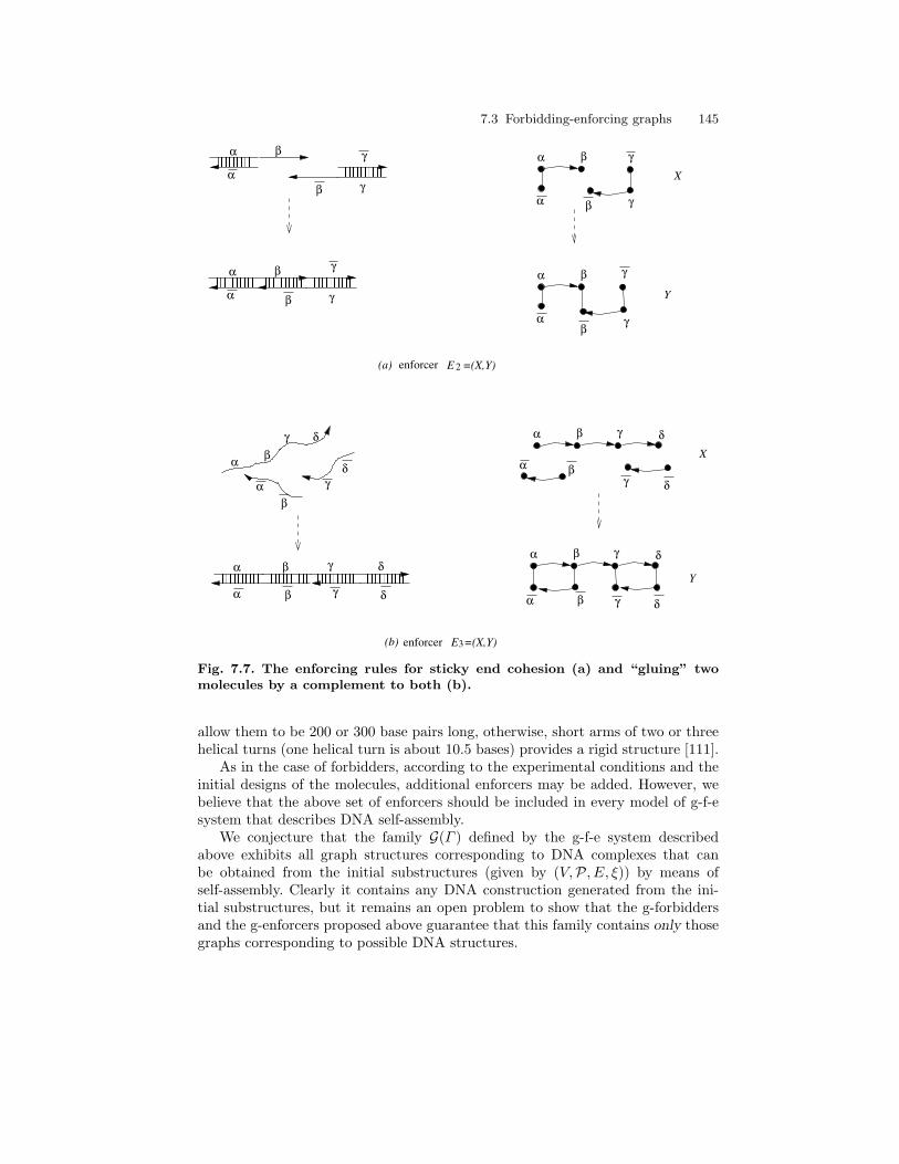
7.3 Forbidding-enforcing graphs 145
������������������
��������������������������������������������
�������������������� ���������������������� ���������
����������������������������������������
� � � � � � � � ������������������������������������������������������
����������������������������������������α β
γ
β
����α
����γ
������δα β
γ δ ����α β
γ
����δ
α β γ δ
����α ��� β
!�!�!"�"γ
#�#$δ
α β γ δ
%�%�%β
&�&γ'�'(
αγ
α β
)�)�)α *�*+β
,�,γα β
γ
α β γ δ
-�-.α /�/�/β γ δ
0�0�0α
γ
1�1�12�2β
α β
γ
X
Y
(a)
X
Y
enforcer
enforcer(b) 3E =(X,Y)
2E =(X,Y)
α 3�34β
5�5γ
Fig. 7.7. The enforcing rules for sticky end cohesion (a) and “gluing” twomolecules by a complement to both (b).
allow them to be 200 or 300 base pairs long, otherwise, short arms of two or threehelical turns (one helical turn is about 10.5 bases) provides a rigid structure [111].
As in the case of forbidders, according to the experimental conditions and theinitial designs of the molecules, additional enforcers may be added. However, webelieve that the above set of enforcers should be included in every model of g-f-esystem that describes DNA self-assembly.
We conjecture that the family G(Γ ) defined by the g-f-e system describedabove exhibits all graph structures corresponding to DNA complexes that canbe obtained from the initial substructures (given by (V,P, E, ξ)) by means ofself-assembly. Clearly it contains any DNA construction generated from the ini-tial substructures, but it remains an open problem to show that the g-forbiddersand the g-enforcers proposed above guarantee that this family contains only thosegraphs corresponding to possible DNA structures.

146 7 A Model for DNA Self-Assembly
Fig. 7.8. Structured junctions starting from three, four, five, six paths ad hocdesigned. The dot line indicates the sticky end rule allowed by E2. Figure on the topleft is a 3-junction. The other ones are structured junctions allowed by E3.
Taking in account that the labels of the vertices are strings over a finite al-phabet, one can consider theoretical questions in the context of formal languagetheory. It may be interesting to investigate the classes of graphs generated by ag-f-e system where the labels of V belong to a given language taken from one ofthe Chomsky classes. On the other hand, considering finite languages and investi-gating how the structure of generated graphs depends on the g-f-e system could beuseful for the study of cellular processes, where for example the function of signaltransduction nets is fairly well understood.
The content of this chapter was entirely published in the following articles.
• G. F., N. Jonoska, Forbidding-Enforcing Conditions in DNA Self-Assembly, J.Chen, N. Jonoska, G. Rozenberg eds: Nanotechnology, Science and Computa-tion, pp 105 - 118, December 2005.
• G. F., N. Jonoska, Forbidding-enforcing graphs for self-assembly, 36th South-eastern International Conference on Combinatorics, Graph Theory, and Com-puting. Congressus Numerantium 177, pp 51 - 63, 2005.
8
Conclusions and Ongoing Research
The important thing is not to stop questioning.Curiosity has its own reason for existing.
Albert Einstein1
The idea of unconventional computing has fired many imaginations, and manyresearchers regard it as a revolution in information processing [31]. In this respect,several directions are addressed in the first chapter of this thesis. An overviewabout molecular computing is given, in terms of state of the art and main problemsfaced, and conclusive notes are proposed along with bibliographical references andcuriosities provoked by a few questions I was asked.
In Chapter 2 algorithmic features of DNA forms are presented from differentviewpoints. The abstract and information-based logic underlying DNA structureseems to be paradigmatic in suggesting a general perspective of investigation,where computational aspects offer research inspirations both to biology and tocomputer science. Three string duplication algorithms are considered and com-pared. In particular, a ‘bilinear duplication algorithm’ is extended to a DNA-likecomputational system based on rewriting rules applied to double strings. Thissystem is just a nice way to show how everything can be computed by suitablycombining the actions of few enzymes on DNA double strings; but it could be astep forward, although on a theoretical level, in the purpose to manipulate naturalprocesses to perform (universal) computations. On the other hand, the relativesimplicity of the biological phenomena we use for this computation, points at thefact that most probably, natural phenomena are much more complex and mayinvolve universal-like computations more often than what we suspect.
Molecular computations are then observed as transformations of objects insideand across the compartments of a membrane system. In this respect, a recentlyintroduced strategy of rule application is recalled, that drops the idea of individualobjects in favour of that of a dynamically controlled evolution of populations. Inthis context, the immunological process of selective leukocyte recruitment is briefly
1 What I Believe, 1930.

148 8 Conclusions and Ongoing Research
described by a membrane system, and then simulated by a program implementingsuch a strategy of membrane rule application.
The middle chapters are essentially the core of the thesis. A variant of thePolymerase Chain Reaction, called XPCR, is introduced to implement null con-text splicing rules on DNA strings. This was experimentally tested in differentsituations, as implementation basis for algorithms of generation, extraction, andmutagenesis, and the laboratory experiments are reported in Chapter 6. The simpletechnology of this approach is interesting in itself, and it has different applicationsin biological contexts, beyond the DNA computing problems that have motivatedit. It takes the advantages and the efficiency of an enzymatic elongation technique,and, it proves convenient with respect to the standard methods in terms of speedand feasibility.
XPCR-based algorithms turned out to be easy-to-implement methods sup-ported by interesting mathematical facts. An analysis of the PCR process is pre-sented in Chapter 3, where a novel extraction method based on XPCR procedure isproposed. This was successfully tested by the experiments described in Section 6.3.Its performance has been then improved, at least at a theoretical level, in [150],where a variant avoiding formations of chimers was introduced, together with theXPCR based mutagenesis algorithm that is described in Chapter 5.
In Chapter 4, we develop a XPCR-based method for implementing parallelsingle-point crossover, in order to generate combinatorial libraries of DNA strands,for DNA computation or other applications needing a similar library of DNAstrands. The method proposed is not the first method for in vitro crossover tobe proposed in DNA-based computing. Namely, parallel overlap assembly (POA)implements hybridization/polymerase extension-based crossover between homolo-gous sequences: a comparison with our method is analyzed in Section 4.5.
A main difference is that, for a mixture of strands, and by employing the usualDNA polymerase, the XPCR method does not suffer of the competition whichaffects POA, because the recombination step of XPCR is defined in such a waythat the two recombining portions have just a codeword in common. Therefore,hybridization between complementary regions (and polymerase extension) maycorrectly occur at only one point. Indeed, if mismatches occur at other points,this can be immediately detected because of a different (from the initial) length ofproduct strings. Our method requires more steps than POA (which requires just1 or 2, while our algorithm requires a linear number of steps) but it proves muchmore convenient from different points of view. Namely, we have less unwanted sideproducts, and we can test the completeness of our library. This is a novelty withrespect to all other generation methods. In this respect, combinatorial propertiesof strings from a pool produced by implementing the XPCR-based quaternaryalgorithm of generation have been proven in Sections 4.2 and 4.3. The algorithmand all the related combinatorial results have been generalized in Section 4.4 tothe generation of non-binary libraries.
The algorithm of ‘quaternary recombination’ is implemented by a polymeraseextension, which is a very efficient enzyme elongation method. This was tested bythe experiment reported in Section 6.4, that showed the potential of the method.However, more experimental results are to be obtained to assess the scalability ofthe algorithm.

8 Conclusions and Ongoing Research 149
The theoretical design of an algorithm to solve an instance of SAT with sig-nificant dimension is described in Chapter 5. It follows the traditional, exhaustivesearch of solutions. Its generation procedure starts from only two strings and re-quires less steps than the quaternary recombination algorithm (log n versus n).Its extraction algorithm is implemented by a combination of polymerase extensionand restriction endonuclease action (cutting operations). This algorithm may havea significant impact in the DNA computing area, because it potentially improvesthe existing methods to perform generating and extracting steps of the traditionalextract model.
Finally, the model for self-assembly which is proposed in Chapter 7 suggestsnew directions both in graph theory and in DNA self-assembly. The general prob-lem here faced is the following: given a set P of paths and cycles, a set F offorbidden structures, and a set E of enforced structures, what are the graphs in-cluded in the set G(Γ ) for Γ = (V,P, E, λ,F , E)? We extend the basic idea ofthe forbidding enforcing systems, that were introduced as unconventional modelof molecular processes in [55], to characterize graphs of (mathematical and biolog-ical) interest.
In particular, the presented model focuses on DNA self-assembly and the setof structures obtained through this process. However, the idea of graph forbiddingenforcing systems can certainly be extended to other self-assembly processes innature as well as in the pure theoretical methods to study mathematical propertiesof graphs. In the case of DNA self-assembly, the evolution process is described ina very natural way as an increase of the cardinality of the matching set betweenvertices with complementary labels. For other types of applications the conceptof g-f-e systems may need to be adjusted in a different way, that would be moresuitable to simulate the evolution in those particular processes.
Coming back to DNA computing, we point out that there has been so far littleprogress towards demonstrating a DNA computation that cannot be trivially per-formed in conventional machines. It is a very important open question to decidewhether DNA computing will at some point reach the level of being useful froma practical point of view. On the other hand, the ultimate goal is not restrictedto the study of realistic systems, implementable today or in the immediate future.The aim rather is to look for plausible computers and for models of them. In fact,progress in technology, whether physical or biochemical, is so rapid (and unpre-dictable) that it would be unwise to limit consideration to knowledge and toolsthat are available today (or tomorrow) [31].
My current research is essentially comprised of two main themes, which are de-scribed in the next sections along their very first results. One is that of looking fora good algorithm to silence genes, what we could call “DNA silencing” (collabora-tion with Vincenzo Manca, University of Verona). The other one is the modelling(by a membrane system) of a particular (unknown enough) phenomenon regardingthe knee arthritis, in order to understand its basic dynamics (collaboration withNatasa Jonoska, USF). Besides, a paper with Vincenzo Manca, Cinzia Giagulliand Carlo Laudanna (University of Verona), has been recently completed [150],where a formal notation and ‘uniformity principles’ are introduced from which theXPCR-based methods follow.
150 8 Conclusions and Ongoing Research
8.1 DNA silencing
In Section 3.4 we faced the following problem. Extracting from a pool P all thestrings including a given substring γ; that is, obtaining a pool composed by all thestrings belonging to P such that contain γ as a substring:
{αγβ | αγβ ∈ P}.
We proposed the XPCR based extraction algorithm that amplifies all the γ-superstrands by means of XPCRγ .
Let us consider now the following ‘complementary’ problem. Given a string γ,extracting all strands from the pool P but γ. In other words, silencing the γ-genefrom a heterogeneous pool of genes, and obtaining a pool composed by all thestrings belonging to P but γ:
P \ {γ}.
Without loss in generality, we can assume that the strings of P have the samelength n. We are looking for a possibly efficient algorithm solving the above ‘silenc-ing problem’, and for example one could think of the following three algorithmicsolutions.
1. By elongation.
Let γ1 and γ2 be the flanking strings of γ, meaning that γ = γ1ξγ2 for somestring ξ. Let δ be a string “sufficiently long”, say 20bp. The γ-genes are canbe detected by performing the following algorithm.a) P := PCR(γ1, γ2δ)(P )b) P := Eln(P )In fact, with a certain number of PCR steps, in (a) all the γ-genes are elongatedby means of a PCR with an external primer (see Section 3.1). Afterwards, theyhave length n+ |δ|, and they can be detected and eliminated from P by lengthselection (an electrophoresis). The idea of elongating all the γ-strings could beperformed also by mutagenesis, by inserting a ‘sufficiently long’ string in somepoint of the sequence γ.
2. By complementarity.
Let γ = γ1ξγ2, with ξ a ‘very short’ string, and let ζ be a ‘very long’ string.The following algorithm detects γ-strings by complementarity, by means of‘bubble’ annealing of them with longer strings (for details on such a kind ofannealing see [235]), that makes them heavier and separable by electrophoresis.A schematic representation of the pool P after the first three steps is displayedin Figure 8.1.a) P := P ∪ {γ1ζγ2}b) P := H(P )c) P := C(P )d) P := Eln(P )

8.1 DNA silencing 151
ζ
γ 1
γ1 γ2
ξ γ 2
γ2
γ1
ξ
γ
γ2
1
χζ
χ=γ ξ=ζ
Fig. 8.1. Silencing by complementarity.
Selection by complementary is not very efficient though [1], and many γ-stringscould remain unattached by the long ones.
3. By blocking PCR.
Let us suppose that all strands of the pool have been previously elongated by aprefix α and a suffix β. Note that they still have the same length n+ |α|+ |β|.Let γ = αγ1ξγ2β, and two corresponding blocking primers η1 = γ1δ, withδ 6= ξ, and η2 = γ2ζ, with ζ 6= ξ.If we perform a special kind of PCR with four primers, two common to all thestrings, and two blocking primers for γ, then all the strings of the pool areamplified but γ. In this case, the algorithm solving the silencing problem isjust the operation:
P := PCR(α, η1, η2, β)
meaning that a PCR with primers α, η1, η2, β is performed. The idea of block-ing primers put at work is depicted in Figure 8.2. One may easily figure outthat the above PCR amplify all the strings but those where η1 and η2 (onlypartially) attach, so blocking the polymerase primer extension.
γ
γ
η
α η
β2
Blocking primers
1
Fig. 8.2. Silencing by blocking.
First experiments have been carried on (during the writing of this thesis) totest the validity of blocking PCR, and quite encouraging results have showed up.

152 8 Conclusions and Ongoing Research
In Figure 8.3 there are the electrophoresis results of tests performed on five pools,four homogeneous (i.e., containing the only string αγβ to silence) called P1, P2,P3, P4, and one heterogeneous called Pt.
In the pool P1 we had S1 as template 2 and we exploited (η1, η2) as cor-responding blocking primers3, in P2 we had S2 as template 4 with (η3, η4) ascorresponding blocking primers5, in P3 we had S3 as template6 having (η5, η6)as blocking primers7, and in P4 there was S4 template8 with (η7, η8) as blockingprimers9. The pool Pt contained S1, S2, S3, S4, and the silencing was performed forall the sequences, by carrying on a blocking PCR with all the regular and blockingprimers (see Figure 8.3). To increase the probability that blocking primers attachfirst than regular primers α and β10, it is enough that they have a higher meltingtemperature (see Section 6.1).
Afterwards, we wondered if the silencing power of the blocking primers coulddepend on the primers concentration. Therefore, more experiments were carriedout on Pt, again with all the blocking primers, but at different concentrations.It seemed to us that no substantial differences can be relieved (see Figure 8.4),thus the method would not depend significantly on primer (and blocking primer)concentrations.
8.2 On modelling knee injuries by membrane systems
We are interested to describe, in abstract and simplified terms, what happens in theknee tissue after an (internal) injury. It is not a well known phenomenon, and wefocus some very recent experimental results that have stimulated our imaginationand our interest. From the experiment described in Section 8.2.2 and carried onat the Medical School of University of South Florida, the interaction between apolymer called hyaluronan and its principal cell receptor seems quite relevant tounderstand some membrane modifications and the cell migration process. Also,at a molecular level, it is not known what is broken by an injury in the system.Therefore, as a starting point to model this phenomenon, in Section 8.2.3 we
2 S1 = GCAGTCGAAGCTGTTGATGCAAGAGATGGTCGTCTGCTAGCATGTCACGAATTAAT-
TAATTAACCACGGAACGGTGAGCGCGAAGACGCTGCCGTAGTCG.3 η1 = CAAGAGATGGTCGTCTGCTAGCATGTCACGCCCCCCCCCCCCCCCCC, η2 =
TCGCGCTCACCGTTCCGTGGCCCCCCCCCCCCCCCCC.4 S2 = GCAGTCGAAGCTGTTGATGCAATGATCTGATCCGTCCCGTTTAAATTTAAATTATA-
AGCAAGTCAGATTGACCGCACGTAACTAGACGCTGCCGTAGTCG.5 η3 = CAATGATCTGATCCGTCCCGCCCCCCCCCCCCCCCCC, η4 = AGTTACGTGCGGT-
CAATCTGACTTGCTTATCCCCCCCCCCCCCCCCC.6 S3 = GCAGTCGAAGCTGTTGATGCAAGATATGGCCCGATTAGTACAGCTACTGAAAATTT-
TAAAATTATAAGTTCCGTCGCTCCGACAGACGCTGCCGTAGTCG.7 η5 = CAAGATATGGCCCGATTAGTACAGCTACTGCCCCCCCCCCCCCCCCC, η6 = GTCG-
GAGCGACGGAACTTATCCCCCCCCCCCCCCCCC.8 S4 = GCAGTCGAAGCTGTTGATGACCTATCAGCCGGCTTGCACAAAAAAAAAAAAAAACT-
CGTATTGTCACGCATCGGTACGTAACTAGACGCTGCCGTAGTCG.9 η7 = ACCTATCAGCCGGCTTGCACCCCCCCCCCCCCCCCCC , η8 = AGTTACGTACCGAT-
GCGTGACAATACGAGTCCCCCCCCCCCCCCCCC.10 α = GCAGTCGAAGCTGTTGATG, β = CGACTACGGCAGCGTCT.
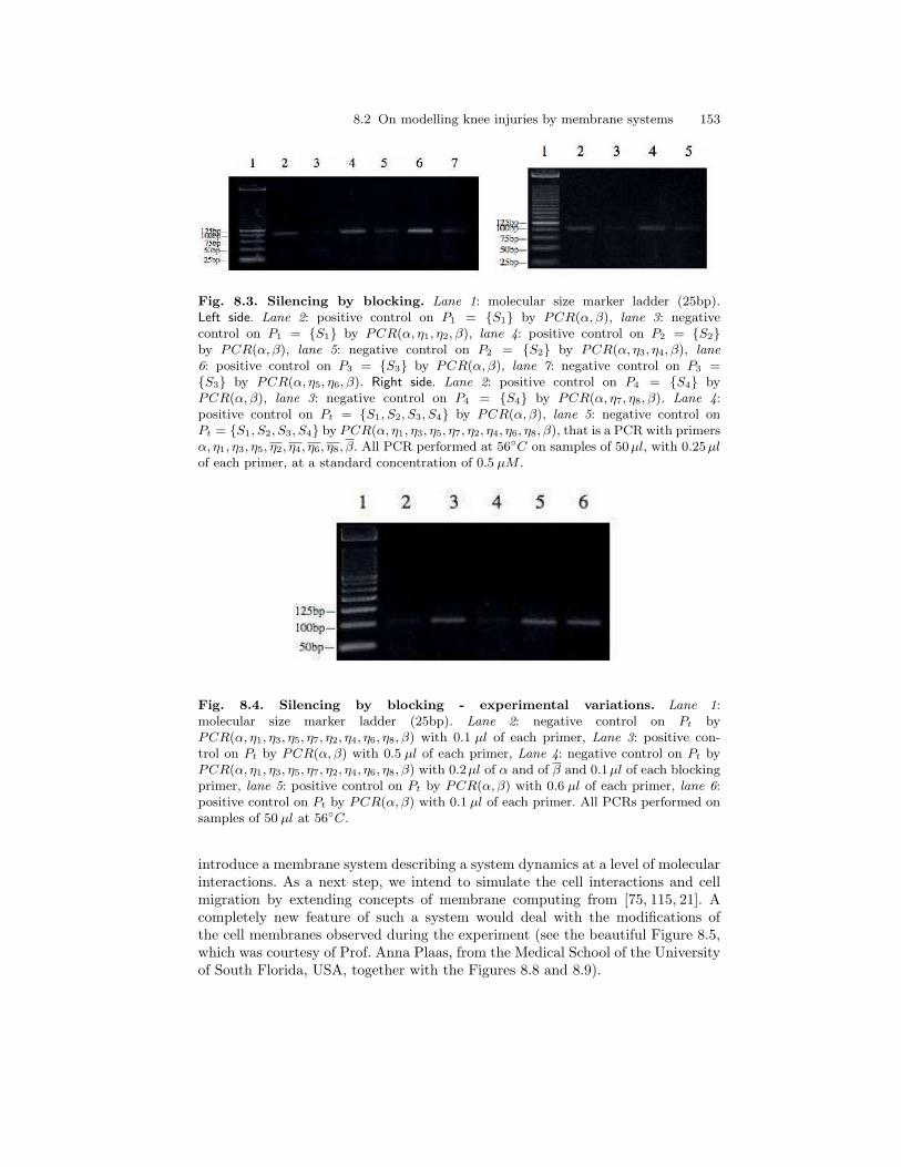
8.2 On modelling knee injuries by membrane systems 153
Fig. 8.3. Silencing by blocking. Lane 1: molecular size marker ladder (25bp).Left side. Lane 2: positive control on P1 = {S1} by PCR(α, β), lane 3: negativecontrol on P1 = {S1} by PCR(α, η1, η2, β), lane 4: positive control on P2 = {S2}by PCR(α, β), lane 5: negative control on P2 = {S2} by PCR(α, η3, η4, β), lane6: positive control on P3 = {S3} by PCR(α, β), lane 7: negative control on P3 ={S3} by PCR(α, η5, η6, β). Right side. Lane 2: positive control on P4 = {S4} byPCR(α, β), lane 3: negative control on P4 = {S4} by PCR(α, η7, η8, β). Lane 4:positive control on Pt = {S1, S2, S3, S4} by PCR(α, β), lane 5: negative control onPt = {S1, S2, S3, S4} by PCR(α, η1, η3, η5, η7, η2, η4, η6, η8, β), that is a PCR with primersα, η1, η3, η5, η2, η4, η6, η8, β. All PCR performed at 56◦C on samples of 50µl, with 0.25µlof each primer, at a standard concentration of 0.5 µM .
Fig. 8.4. Silencing by blocking - experimental variations. Lane 1:molecular size marker ladder (25bp). Lane 2: negative control on Pt byPCR(α, η1, η3, η5, η7, η2, η4, η6, η8, β) with 0.1 µl of each primer, Lane 3: positive con-trol on Pt by PCR(α, β) with 0.5 µl of each primer, Lane 4: negative control on Pt byPCR(α, η1, η3, η5, η7, η2, η4, η6, η8, β) with 0.2µl of α and of β and 0.1µl of each blockingprimer, lane 5: positive control on Pt by PCR(α, β) with 0.6 µl of each primer, lane 6:positive control on Pt by PCR(α, β) with 0.1 µl of each primer. All PCRs performed onsamples of 50 µl at 56◦C.
introduce a membrane system describing a system dynamics at a level of molecularinteractions. As a next step, we intend to simulate the cell interactions and cellmigration by extending concepts of membrane computing from [75, 115, 21]. Acompletely new feature of such a system would deal with the modifications ofthe cell membranes observed during the experiment (see the beautiful Figure 8.5,which was courtesy of Prof. Anna Plaas, from the Medical School of the Universityof South Florida, USA, together with the Figures 8.8 and 8.9).
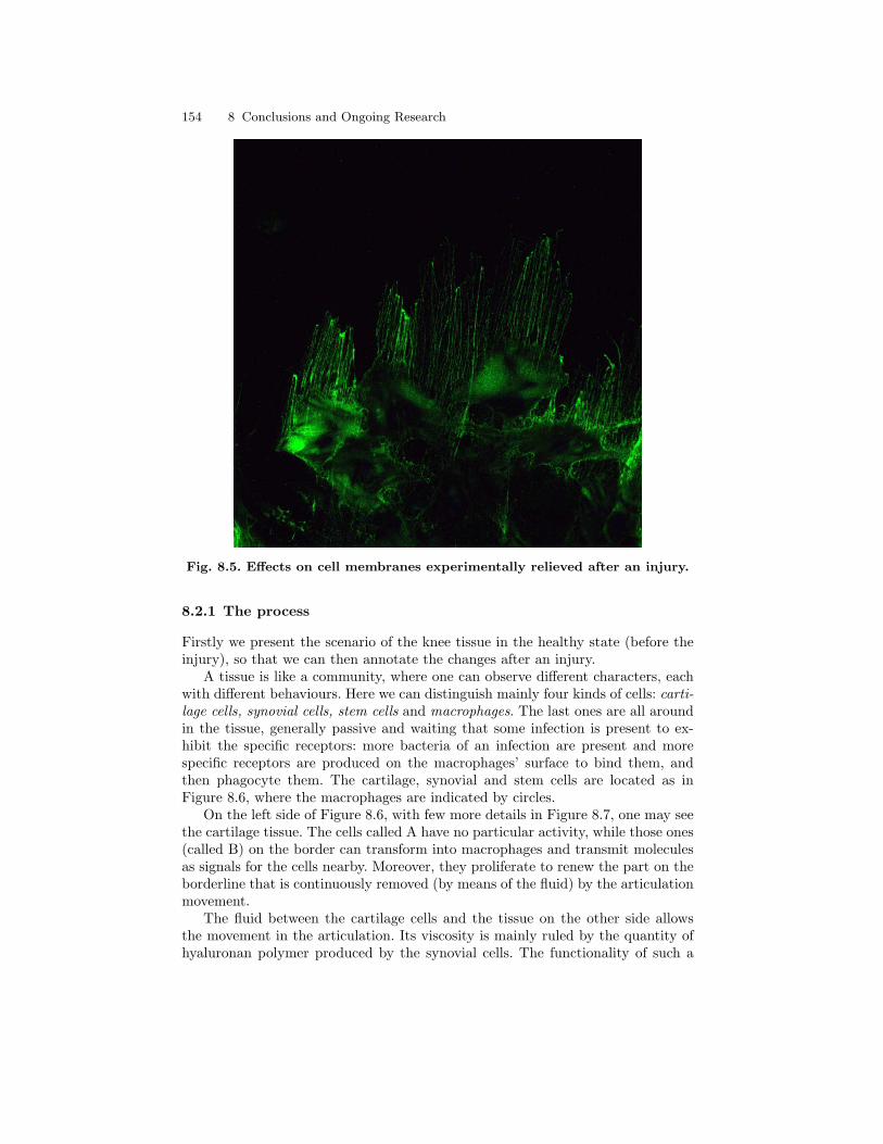
154 8 Conclusions and Ongoing Research
Fig. 8.5. Effects on cell membranes experimentally relieved after an injury.
8.2.1 The process
Firstly we present the scenario of the knee tissue in the healthy state (before theinjury), so that we can then annotate the changes after an injury.
A tissue is like a community, where one can observe different characters, eachwith different behaviours. Here we can distinguish mainly four kinds of cells: carti-lage cells, synovial cells, stem cells and macrophages. The last ones are all aroundin the tissue, generally passive and waiting that some infection is present to ex-hibit the specific receptors: more bacteria of an infection are present and morespecific receptors are produced on the macrophages’ surface to bind them, andthen phagocyte them. The cartilage, synovial and stem cells are located as inFigure 8.6, where the macrophages are indicated by circles.
On the left side of Figure 8.6, with few more details in Figure 8.7, one may seethe cartilage tissue. The cells called A have no particular activity, while those ones(called B) on the border can transform into macrophages and transmit moleculesas signals for the cells nearby. Moreover, they proliferate to renew the part on theborderline that is continuously removed (by means of the fluid) by the articulationmovement.
The fluid between the cartilage cells and the tissue on the other side allowsthe movement in the articulation. Its viscosity is mainly ruled by the quantity ofhyaluronan polymer produced by the synovial cells. The functionality of such a

8.2 On modelling knee injuries by membrane systems 155
cartilagecells
cartilage
cells
fluidcells
stemcells
macrophages
synovial
Fig. 8.6. The knee tissue nearby joints in a healthy state.
viscosity is controversial, especially for its role in tumor progression and metastasis,but in this context we can assume that in the healthy state we have an equilibratedquantity of hyaluronan, enough to hydrate and to feed the neighboring cells andto take away their waste products.
The most intriguing part of this zoom is on the right side of Figure 8.7, wheresynovial and stem cells are located. In a healthy state the stem cells just performtheir turn-over: slightly proliferating and producing collagen, they die by apoptosis(gradual death). The synovium is a thin, weak layer of tissue only a few cells thickwhich lines the joint space. It acts to control the environment within the joint. Itdoes this in two ways: first, it acts as a membrane to determine what can passinto the joint space and what stays outside; second, the cells within the synoviumsecrete substances, such as hyaluronan, which are the components of joint fluid.
After an injury, proliferation rates increase and new processes of cell differen-tiation and migration are activated by molecular signalling.
We can consider the total number of cells involved in this phenomenon un-limited, because they all can proliferate, and generally the cells are not terminallydifferentiated. In particular, a stem cell can transform into a synovial cell and theninto a cartilage cell. The differentiation of cells happens mainly along the directionright-left in Figure 8.7, because the ultimate goal of the process is the reparation ofthe knee articulation. Cell differentiation and migration can be considered simul-taneous, in fact the areas indicated in Figures 8.6 and 8.7 remain approximatelythe same during the whole process. For this reason we will identify such areas withregions of membranes.
New cartilage cells, forming the scar tissue, are thus produced after an injuryand they are finally located all around the old cartilage cells (a similar phase
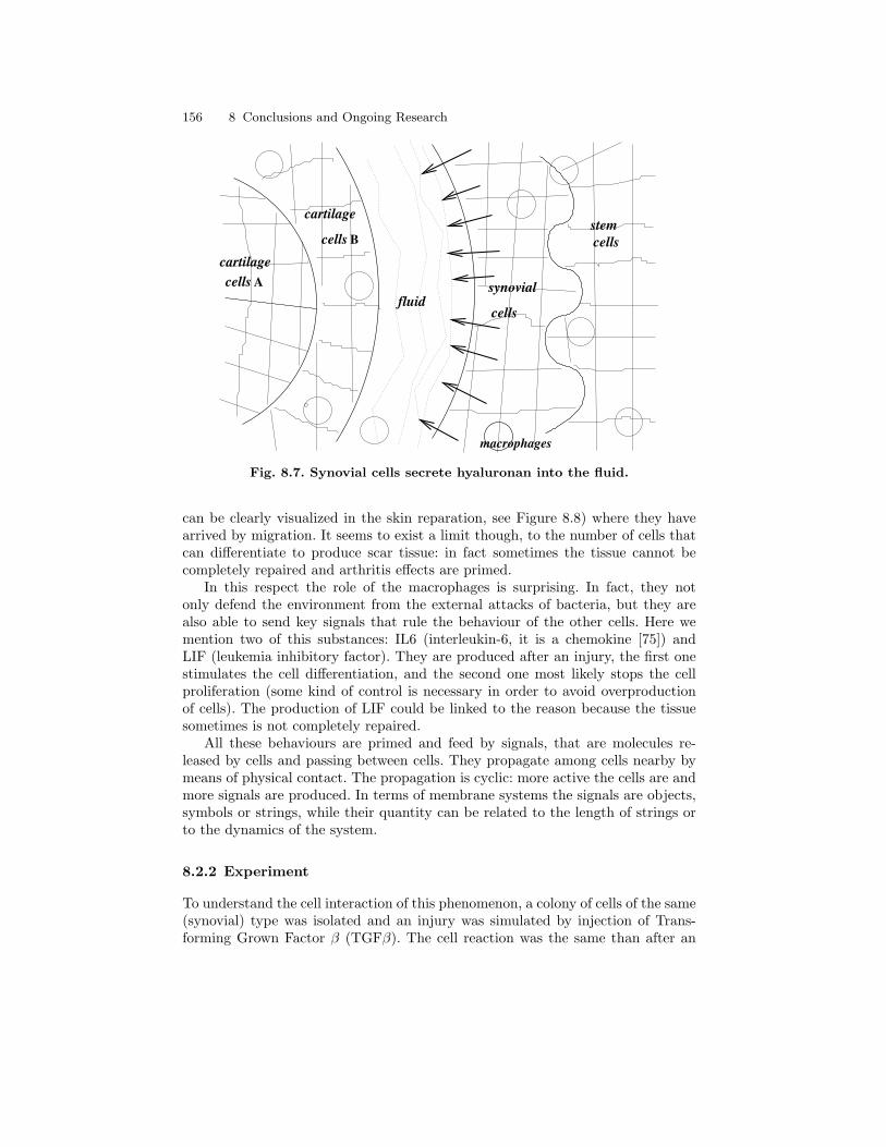
156 8 Conclusions and Ongoing Research
cartilagecells
cartilage
cells
fluidcells
stemcells
macrophages
B
A synovial
Fig. 8.7. Synovial cells secrete hyaluronan into the fluid.
can be clearly visualized in the skin reparation, see Figure 8.8) where they havearrived by migration. It seems to exist a limit though, to the number of cells thatcan differentiate to produce scar tissue: in fact sometimes the tissue cannot becompletely repaired and arthritis effects are primed.
In this respect the role of the macrophages is surprising. In fact, they notonly defend the environment from the external attacks of bacteria, but they arealso able to send key signals that rule the behaviour of the other cells. Here wemention two of this substances: IL6 (interleukin-6, it is a chemokine [75]) andLIF (leukemia inhibitory factor). They are produced after an injury, the first onestimulates the cell differentiation, and the second one most likely stops the cellproliferation (some kind of control is necessary in order to avoid overproductionof cells). The production of LIF could be linked to the reason because the tissuesometimes is not completely repaired.
All these behaviours are primed and feed by signals, that are molecules re-leased by cells and passing between cells. They propagate among cells nearby bymeans of physical contact. The propagation is cyclic: more active the cells are andmore signals are produced. In terms of membrane systems the signals are objects,symbols or strings, while their quantity can be related to the length of strings orto the dynamics of the system.
8.2.2 Experiment
To understand the cell interaction of this phenomenon, a colony of cells of the same(synovial) type was isolated and an injury was simulated by injection of Trans-forming Grown Factor β (TGFβ). The cell reaction was the same than after an

8.2 On modelling knee injuries by membrane systems 157
Fig. 8.8. Reparation by cell differentiation and migration in the bovine skin.
injury. The cells on the tissue surface around an hypothetic injury were stimulatedto line, and the cells reaction was increased by injecting more and more TGFβ.
Some results were a wide production of hyaluronan polymer by the lining cellsand the formation of membrane filaments directed towards the injury side (as inFigure 8.5). Therefore the interruption of the interactions present in the healthystate destabilizes the regular form of the cell surface, but the reason of that is asunknown as appealing. Recent studies11 show that these formations are mainlystimulated and allowed by external environment factors, but they are also pro-duced by the internal pushing of the enzyme producing hyaluronan. Moreover,no differentiation and two kinds of migration processes were relieved during theexperiment, the planar one and the in-deep one, both towards the injury location.
The cellular movement induced by the presence of certain chemicals, towardsthose chemicals, is called chemotaxis. In the culture of the experiment no chemo-tactic locomotion occurred, because the cell migration happened towards the in-jury meanwhile the stimulating substance (TGFβ) was all over. But in the animaltissue, since the TGFβ is produced locally by cells reacting to the injury, a chemo-tactic migration likely happens. Finally, after the ‘injury’ the lining cells in theculture started to proliferate towards the empty space allowed by the injury. Thisreaction could be locally due just to the fact that they found room to proliferate.
An interesting fact to point out here is that the whole role of a cell in a tissueis dictated by external stimulates: what kind of cell it is, its functioning, and itsbehaviour. For example, all the cells have potential to make, bind, and interactwith hyaluronan, but they do it or not depending on the environmental conditions.
In Figure 8.9 one can see the changing form of the cartilage tissue before (onthe left), and after (on the right) the injury, when it needs to be repaired.
The green fluorescence relies the presence of hyaluronan, in fact, in the two fig-ures an increasing production of hyaluronan can be observed. The red fluorescence
11 Kirsi Rilla, Anne Kultti, Andrew Spicer, Raija Tammi and Markku Tammi, Hyaluro-nan synthase and hyaluronan coat on MCF-7 breast cancer cells, Hyaluronan oligosac-charide workshop, Boston, July 17, 2004.

158 8 Conclusions and Ongoing Research
Fig. 8.9. Disposition of the synovial cells before and after the injury.
represents a different substance called lubricin. In a healthy state it is generallyproduced by the cartilage cells and retained by the lining (called B) cells, where wecan observe an accumulation (see left part of Figure 8.9). After the injury some-thing happens in such a way that the lubricin is spread out, maybe the productionis interrupted, or maybe the lining cells release it all around.
In the next section, a membrane system is proposed as initial model. Technicaldetails about the interaction between hyaluronan and its cell receptor would helpto better understand the importance and the complexity underlying the wholephenomenon, but we are going slightly under the way.
8.2.3 A membrane system
The changes of the two main molecular productions observed during the experi-ment, regarding lubricin and hyaluronan, are here presented in a very schematicmanner.
Let us identify the TGFβ with the symbol s (as starting the process after aninjury), the hyaluronan with h, and the lubricin with l. Let us consider the twosides of an injury as nested membranes in which one can simulate the progressiveaction of the substance-symbol s over the cells in the most internal layers. Thequantity of TGFβ is given by the length of the input string. The proper regionof each membrane represents the layer of cells of a certain type, and the quantityof symbols from {a, b, c, d} present in the initial configuration of the system (forexample two in Figure 8.10) is proportional to the activity and production abilityof the cells in the corresponding area. In a first approximation we have chosenthree layers; the idea is to simulate the distribution of lubricin and hyaluronan inFigure 8.9 with the quantity of symbols l and h respectively.
The membrane M in the initial configuration reminds the presence of macro-phage cells, which have a role in the molecular system. In fact, they produce LIFsubstance which stops the proliferation of the lining cells (corresponding to thearea with symbols c), that is primed by the injury.

8.2 On modelling knee injuries by membrane systems 159
M
sssssssss
sssss
c
c
c
c
b
ba
a
b
b
a
a
Fig. 8.10. Initial configuration of the membrane system simulating lubricin and hyaluro-nan production.
We propose the following global rules (i.e., unspecific for any region) on the al-phabet {a, b, c, c′, l, h, s}, that transform and exchange objects between membraneregions. We recall the semantic of the rules: the premises are transformed in theproducts by the rule wherever the premise symbols occur all together, while hereand in indicate the region destination for objects introduced by the evolution rules.In particular, (ξ, in) means that ξ will enter any of the adjacent lower region (ifthere is any), chosen nondeterministically among all adjacent lower regions [180].For example, after the application of the following first rule, a symbol s has enteredone of the two bigger membranes of the system in Figure 8.10.
s s s s→ (s s s, here) (s, in)a→ (a, here) (l, out)b → (b, here) (l, out)b l → (b, here) (l, out)
s s c l → (s s c c′, here) (l, in)s s a→ s ss s b → s s
c→ c hc′ → (c′ h, here) (h h, out)
In this context the structure of string is not relevant, it just means the simul-taneous presence of its elements. The application of the rules is nondeterministicand maximally parallel as usual; for example, if b, b, l are all present in a sameregion, then both the third and fourth rule are applied, and both the symbol l andan extra copy of it are sent out of that membrane.
The first rule simulates the progressive entry of the symbol s into the tissueand then into the most internal membranes. A layer can be passed through by thesubstance when it contains at least three copies of s (for example). The second,third, and fourth rules simulate the production of lubricin from the most internallayers, and its accumulation into the external one of the tissue, as happens duringthe healthy state (left part of Figure 8.9). The fifth rule simulates the releaseof lubricin by the lining cells after an injury, while the sixth and seventh rules
160 8 Conclusions and Ongoing Research
represent the slowing down of lubricin production. The last two rules simulaterespectively the regular and then increasing production of hyaluronan after aninjury.
This system is in a very infantile stage, it still needs to be tested and improved.Moreover, while setting a good molecular system, we should take in account thatmolecular productions are related to proliferation and differentiation processes. Infact, after an injury, the lining cartilage cells start to proliferate (as a consequencethe molecular production of these cells increase tremendously) and to differen-tiate in macrophages, meaning that the number of cells sending signals to stopproliferation and to stimulate differentiation increases as well.
We wonder if the molecular production happening during cell proliferation anddifferentiation can be simulated only by evolution rules of objects. If a cell generatestwo cells producing a copy of the substance p, the quantity of p after n steps is20 + 21 + · · · + 2n = 2n+1 − 1. Moreover, these productions are “auto-ruled”, asdifferentiation can occur, and differentiation in macrophages for example increasesthe production of substances that stop the proliferation.
Next goals for this modelling work are i) to define general rules that simulatethe behaviour of healthy and injured tissue at the same time, ii) once the rulesare established to identify some computational behaviour of the system (such asproduction of languages), iii) to identify good experimental conditions that willhelp to learn more precise rules of the system.
As final remarks, we point out the following observations related to this workwith respect the membrane computing literature. The region of a membrane hererepresents a layer of cells of a certain type. In order to describe some phenomena,the differentiation and the movement (migration) of membranes should be allowedin a membrane system (a recent work in this direction is [17]). The cell membranescan change their form! In fact, as an experimental result, the interruption of theinteractions present in the healthy state destabilizes the regular form of the cellsurface (this is a consequence of the receptor-receptor interaction, a concept al-ready formalized in modelling biological processes by membrane systems [75] andstudied from a computational perspective [17]).
As a future research, I would like to carry on more experiments testing thescalability of the XPCR-based (extraction, generation, mutagenesis) methods in-troduced in Chapters 3, 4, and 6. An implementation in laboratory of the algo-rithm solving SAT proposed in Chapter 5 would be pretty interesting as well.In general, I’m interested in designing models and algorithms involving biologicalstrings interactions—namely by investigating possible applications of the notionof DNA blocking introduced in Chapter 8 or by extending the self-assembly modelpresented in Chapter 7. Finally, as a modelling work, I intend to develop themodel for reparation of knee injuries12 presented in Chapter 8, and to continuethe work [75] with (my advisor) Vincenzo Manca, by investigating immunologi-cal processes both from molecular (for example the genetic recombination of theipervariable regions of antibodies) and cellular viewpoint.
12 supported by the kind collaboration of Natasa Jonoska from Mathematics Department,Barbara Osborn and Anna Plaas from Medical School, of USF, USA.
References
1. L. M. Adleman. Molecular Computation of Solutions to Combinatorial Problems.Science, 266(5187):1021–1024, 1994.
2. B. Alberts, A. Johnson, J. Lewis, M. Raff, K. Roberts, and J. D. Watson. MolecularBiology of the Cell. Garland Science, New York, fourth edition, 2002.
3. A. Alhazov, R. Freund, and Gh. Paun. Computational Completeness of P Sys-tems with Active Membranes and Two Polarizations. In M. Margenstern, editor,Machines, Computations, and Universality, International Conference, MCU 2004,Saint Petersburg, 2004, Revised Selected Papers, volume 3354 of Lecture Notes inComputer Science, pages 82–92. Springer, 2005.
4. M. Amos. DNA Computation. PhD thesis, University of Warwick, UK, Sept 1997.5. M. Amos. Theoretical and Experimental DNA Computation. Natural Computing
Series. Springer, 2005.6. A. Animashree, K. Krithivasan, and A. Choudhary. Breaking DES Using Peptide-
Antibody Interactions. In A. Carbone, M. Daley, L. Kari, I. McQuillan, andN. Pierce, editors, Pre-proceedings of DNA 11:. The 11th International Meetingon DNA Computing, June 6-9 2005, London, Ontario, Canada, page 389, 2005.
7. I. Ardelean, D. Besozzi, M. H. Garzon, G. Mauri, and S. Roy. P System Models forMechanosensitive Channels. In [43], chapter 2, pages 43–82. Springer, 2006.
8. M. Arita. Writing Information into DNA. In [117], pages 23–35, 2004.9. P. Arrighi. Quantum Computation Explained to my Mother. Bulletin of EATCS,
80:134–142, June 2003.10. B. Aspvall, M. F. Plass, and R. E. Tarjan. A Linear-Time Algorithm for Testing
the Truth of Certain Quantified Boolean Formulas. Information Processing Letters,8(3):121–123, 1979.
11. M. S. Balan, K. Krithivasan, and Y. Sivasubramanyam. Peptide Computing - Uni-versality and Complexity. In [120], pages 290–299, 2002.
12. N. Barbacari, A. Profir, and C. Zelinschi. Gene Regulatory Network Modellingby Means of Membrane Systems. In R. Freund, G. Lojka, M. Oswald, and Gh.Paun, editors, Pre-proceedings of the 6th International Workshop on MembraneComputing, July 18-21 2005, Vienna, Austria, pages 162–178, 2005.
13. E. B. Baum. Building an Associative Memory Vastly Larger than the Brain. Science,268(5210):583–585, 1995.
14. Y. Benenson, T. Paz-Elizur, R. Adar, E. Keinan, Z. Livneh, and E. Shapiro. Pro-grammable and Autonomous Computing Machine made of Biomolecules. Nature,414(1):430–434, 2001.
15. C. H. Bennett. Logical Reversibility of Computation. IBM Journal of Research andDevelopment, 17:525–532, 1973.

162 References
16. C. H. Bennett. The Thermodynamics of Computation - a Review. InternationalJournal of Theoretical Physics, 21(12):905–940, 1982.
17. F. Bernardini and M. Gheorghe. Cell Communication in Tissue P Systems: Univer-sality Results. Soft Computing, 9(9):640–649, 2005.
18. F. Bernardini, M. Gheorghe, N. Krasnogor, R. C. Muniyandi, M. J. Perez-Jimenez,and F. J. Romero-Campero. On P Systems as a Modelling Tool for BiologicalSystems. In [81], pages 114–133, 2006.
19. F. Bernardini and V. Manca. P Systems with Boundary Rules. In Gh. Paun,G. Rozenberg, A. Salomaa, and C. Zandron, editors, Membrane Computing: Inter-national Workshop, WMC-CdeA 2002, Curtea de Arges, Romania, August 19-23,2002. Revised Papers, volume 2597 of Lecture Notes in Computer Science, pages107–118. Springer, 2002.
20. F. Bernardini and V. Manca. Dynamical Aspects of P Systems. BioSystems,70(2):85–93, 2003.
21. L. Bianco, F. Fontana, G. Franco, and V. Manca. P Systems for Biological Dynam-ics. In [43], chapter 3, pages 83–128. Springer, 2006.
22. L. Bianco, F. Fontana, and V. Manca. Metabolic Algorithm with Time-VaryingReaction Maps. In Proceedings of the Third Brainstorming Week on MembraneComputing, Sevilla, Spain, pages 43–61, February 2005.
23. L. Bianco, F. Fontana, and V. Manca. P Systems with Reaction Maps. InternationalJournal of Foundations of Computer Science, 17(1):27–48, 2006.
24. L. Bianco and V. Manca. Metabolic Algorithms and Signal Transduction DynamicalNetworks. In First Brainstorming Workshop on Uncertainty in Membrane Comput-ing, Palma de Mallorca, Spain, pages 119–120, November 2004.
25. L. Bianco and V. Manca. Symbolic Generation and Representation of ComplexOscillations. International Journal of Computer Mathematics, to appear(2006).
26. D. Boneh, C. Dunworth, and R. Lipton. Breaking DES Using a Molecular Computer.In [144], pages 37–65, 1995.
27. P. Bottoni, C. Martın-Vide, Gh. Paun, and G. Rozenberg. Membrane Systems withPromoters/Inhibitors. Acta Informatica, 38(10):695–720, 2002.
28. R. S. Braich, N. Chelyapov, C. Johnson, P. W. K. Rothemund, and L. M. Adle-man. Solution of a 20-variable 3-SAT Problem on a DNA Computer. Science,296(5567):499–502, 2002.
29. R. S. Braich, C. Johnson, P. W. K. Rothemund, D. Hwang, N. Chelyapov, and L. M.Adleman. Solution of a Satisfiability Problem on a Gel-Based DNA Computer. In[44], pages 27–41, 2000.
30. K. J. Breslauer, R. Frank, H. Blocker, and L.A. Markey. Predicting DNA DuplexStability from the Base Sequence. Proceedings of the National Academy of Scienceof USA (PNAS), 83(11):3746–3750, 1986.
31. C. S. Calude and Gh. Paun. Computing with Cells and Atoms – An Introductionto Quantum, DNA and Membrane Computing. Taylor and Francis Inc, 2001.
32. A. Carbone and N.A. Pierce, editors. Proceedings of the 11th International Work-shop on DNA Computing: DNA 11, London, Ontario, Canada, June 2005. RevisedSelected Papers, volume 3892 of Lecture Notes in Computer Science. Springer, 2006.
33. A. Carbone and N.C. Seeman. Coding and Geometrical Shapes in Nanostructures:a Fractal DNA-assembly. Natural Computing, 2:133–151, 2003.
34. L. Cardelli. Bitonal Membrane Systems – Interactions of Biological Membranes.Microsoft Research, Cambridge, UK, October 2003.
35. L. Cardelli and A. D. Gordon. Mobile Ambients. Theoretical Computer Science –Special Issue on Coordination, 240(1):177–213, 2000.
36. G. Casiraghi, C. Ferretti, A. Gallini, and G. Mauri. A Membrane Computing SystemMapped on an Asynchronous, Distributed Computational Environment. In [81],pages 159–164, 2006.
References 163
37. M. Cavaliere and N. Jonoska. Forbidding and Enforcing in Membrane Computing.Natural Computing, 2(3):215–228, 2003.
38. M. Cavaliere, N. Jonoska, and P. Leupold. Recognizing DNA Splicing. In [32],pages 12–26, 2006.
39. M. Cavaliere, N. Jonoska, S. Yogev, R. Piran, E. Keinan, and N. C. Seeman.Biomolecular Implementation of Computing Devices with Unbounded Memory. In[64], pages 35–49, 2005.
40. J. Chen, R. Deaton, and Y.-Z. Wang. A DNA-Based Memory with in vitro Learningand Associative Recall. Natural Computing, 4(2):83–101, 2005.
41. J.H. Chen and N.C. Seeman. Synthesis from DNA of a Molecule with the Connec-tivity of a Cube. Nature, 350:631–633, 1991.
42. K. Chen and E. Winfree. Error Correction in DNA Computing: Misclassificationand Strand Loss. In [238], pages 49–62, 2000.
43. G. Ciobanu, Gh. Paun, and M. J. Perez-Jimenez, editors. Applications of MembraneComputing. Natural Computing Series. Springer, 2006.
44. A. Condon and G. Rozenberg, editors. DNA Computing: Proceedings of the 6th In-ternational Workshop on DNA-Based Computers, DNA 2000, Leiden, The Nether-lands, June 13-17, 2000, Revised Papers, volume 2054 of Lecture Notes in ComputerScience. Springer, 2001.
45. M. Conrad. Information Processing in Molecular Systems. Currents in ModernBiology, 5(1):1–14, 1972.
46. M. Conrad. On Design Principles for a Molecular Computer. Communication ofthe ACM, 28:464–480, 1985.
47. E. Csuhaj-Varju, L. Kari, and Gh. Paun. Test Tube Distributed Systems Based onSplicing. Computers and AI, 15(2-3):211–232, 1996.
48. M. Daley and I. McQuillan. On Computational Properties of Template-GuidedDNA Recombination. In [32], pages 27–37, 2006.
49. J. Dassow and V. Mitrana. Splicing Grammar Systems. Computers and AI, 15(2-3):109–122, 1996.
50. R. Deaton, J. Chen, H. Bi, M. Garzon, H. Rubin, and D. H. Wood. A PCR-BasedProtocol for In Vitro Selection of Non-Crosshybridizing Oligonucletides. In [95],pages 196–204, 2002.
51. A. DeLuca and A. Restivo. A Characterization of Strictly Locally Testable andits Application to Subsemigroups of a Free Semigroup. Information and Control,44(3):300–319, 1980.
52. R. DeSalle, M. Barcia, and C. Wray. PCR Jumping in Clones of 30-Million-Year-Old DNA Fragments from Amber Preserved Termites. Experientia, 49(10):906–909,1993.
53. D. Dressman, H. Yan, G. Traverso, K. W. Kinzler, and B. Vogelstein. TransformingSingle DNA Molecules into Fluorescent Magnetic Particles for Detection and Enu-meration of Genetic Variations. Proceedings of the National Academy of Science ofUSA (PNAS), 100(15):8817–8822, 2003.
54. A. Ehrenfeucht, T. Harju, I. Petre, D. M. Prescott, and G. Rozenberg. FormalSystems for Gene Assembly in Ciliates. Theoretical Computer Science, 292:199–219, 2003.
55. A. Ehrenfeucht, H. J. Hoogeboom, G. Rozenberg, and N. van Vugt. Forbidding andEnforcing. In [238], pages 195–206, 2000.
56. A. Ehrenfeucht, I. Petre, D. M. Prescott, and G. Rozenberg. String and Graph Re-duction Systems for Gene Assembly in Ciliates. Mathematical Structures in Com-puter Science – Special Issue: Theory and Applications of Graph Transformations,12:113–134, 2002.
164 References
57. A. Ehrenfeucht, D. M. Prescott, and G. Rozenberg. Computational Aspects of Gene(un)scrambling in Ciliates. Evolution as Computation, pages 216–256, 2001.
58. A. Ehrenfeucht and G. Rozenberg. Forbidding-Enforcing Systems. Theoretical Com-puter Science, 292(3):611–638, 2003.
59. T. L. Eng. Linear DNA Self-Assembly with Hairpins Generate the Equivalent ofLinear Context-Free Grammars. In [204], pages 296–301, 1998.
60. T. L. Eng. On Solving 3CNF-satisfiability with an in vivo Algorithm. [125], pages135–141, 1999.
61. D. Faulhammer, A. R. Cukras, R. J. Lipton, and L. F. Landweber. Molecular Com-putation: RNA Solution to Chess Problems. Proceedings of the National Academyof Science of USA (PNAS), 98(4):1385–1389, 2000.
62. D. Faulhammer, R. J. Lipton, and L. F. Landweber. Counting DNA: Estimatingthe Complexity of a Test Tube of DNA. [125], pages 193–196, 1999.
63. C. Ferretti, S. Kobayashi, and T. Yokomori. DNA Splicing Systems and Post Sys-tems. In L. Hunter and T. E. Klein, editors, First Annual Pacific Conference onBiocomputing, pages 288–299. World Scientific, 1996.
64. C. Ferretti, G. Mauri, and C. Zandron, editors. Proceedings of the 10th InternationalWorkshop on DNA Computing: DNA 10, Milan, Italy, June 2004. Revised SelectedPapers, volume 3384 of Lecture Notes in Computer Science. Springer, 2005.
65. R. P. Feynman. Miniaturization. In D. H. Gilbert, editor, Reinhold, pages 282–296.New York, 1961.
66. F. Fontana, L. Bianco, and V. Manca. P Systems and the Modeling of BiochemicalOscillations. In [81], pages 199–208, 2006.
67. F. Fontana and G. Franco. Finding the Maximum Element Using P Systems. Jour-nal of Universal Computer Science, 10(5):567– 580, 2004.
68. G. Franco. Combinatorial Properties of DNA Libraries Generated via Null ContextSplicing Rules. Submitted.
69. G. Franco. Algoritmi DNA per la Soddisfacibilita Proposizionale. Master’s thesis,Dipartimento di Matematica, Universita degli Studi di Pisa, November 2001.
70. G. Franco. Hard Instances of SAT. TR project ‘Biomolecular Algorithms for NP-Complete roblems’, Department of Computer Science, University of Pisa, July 2002.
71. G. Franco. A Polymerase Based Algorithm for SAT. In M. Coppo, E. Lodi, andG. M. Pinna, editors, Theoretical Computer Science, volume 3701 of Lecture Notesin Computer Science, pages 237–250. Springer, 2005.
72. G. Franco, C. Giagulli, C. Laudanna, and V. Manca. DNA Extraction by XPCR.In [64], pages 104–112, 2005.
73. G. Franco and N. Jonoska. Forbidding - Enforcing Conditions in DNA Self-Assembly. In J. Chen, N. Jonoska, and G. Rozenberg, editors, Nanotechnology,Science and Computation, pages 105–118, 2005.
74. G. Franco and N. Jonoska. Forbidding-Enforcing Graphs for Self-Assembly. Con-gressus Numerantium, 177:51–63, 2005.
75. G. Franco and V. Manca. A Membrane System for the Leukocyte Selective Recruit-ment. In C. Martın-Vide, G. Mauri, Gh. Paun, G. Rozenberg, and A. Salomaa,editors, Membrane Computing, Revised Papers of WMC 2003, Tarragona, Spain,volume 2933 of Lecture Notes in Computer Science, pages 181–190. Springer, 2004.
76. G. Franco and V. Manca. An Algorithmic Analysis of DNA Structure. Soft Com-puting, 9(10):761–768, 2005.
77. G. Franco, V. Manca, C. Giagulli, and C. Laudanna. DNA Recombination byXPCR. In [32], pages 55–66, 2006.
78. F. Freund, R. Freund, M. Oswald, M. Margenstern, Y. Rogozhin, and S. Verlan. PSystems with Cutting/Recombination Rules Assigned to Membranes. In C. Martın-Vide, G. Mauri, Gh. Paun, G. Rozenberg, and A. Salomaa, editors, Membrane
References 165
Computing, volume 2933 of Lecture Notes in Computer Science, pages 191–202.Springer, 2004.
79. R. Freund, L. Kari, and Gh. Paun. DNA Computing Based on Splicing: The Exis-tence of Universal Computers. Theory of Computing Systems, 32(1):69–112, 1999.
80. R. Freund, Gh. Paun, G. Rozenberg, and A. Salomaa. Watson-Crick Automata.Techn. Report 97-13, Dept of Computer Science, Leiden University, 1997.
81. R. Freund, Gh. Paun, G. Rozenberg, and A. Salomaa, editors. Membrane Comput-ing, International Workshop, WMC6, Vienna, Austria, 2005, Revised Selected andInvited Papers, volume 3850 of Lecture Notes in Computer Science. Springer, 2006.
82. P. Frisco. Theory of Molecular Computing - Splicing and Membrane Systems.PhD thesis, Leiden Institute of Advanced Computer Science (LIACS), Leiden, TheNetherlands, June 2004.
83. P. Frisco and R. T. Gibson. A Simulator and an Evolution Program for Conformon-PSystems. In Seventh International Symposium on Symbolic and Numeric Algorithmsfor Scientific Computing, pages 427–430. IEEE Computer Society Press, 2005.
84. P. Frisco, C. Henkel, and S. Tengely. An Algorithm for SAT without an ExtractionPhase. In [32], pages 67–80, 2006.
85. R. H. Garrett and C. M. Grisham. Biochemistry. Saunders College Publishing,Harcourt, 1997.
86. M. Garzon, R. Deaton, and D. Reanult. Virtual Test Tubes: A New Methodology forComputing. In Seventh International Symposium String Processing and Informationretrieval, A Coruna, Spain, pages 116–121. IEEE Computing Society Press, 2000.
87. M. H. Garzon, K. V. Bobba, and B. P. Hyde. Digital Information Encoding onDNA. In [117], pages 152–166, 2004.
88. M. H. Garzon, N. Jonoska, and S. A. Karl. The Bounded Complexity of DNAComputing. [125], pages 63–72, 1999.
89. A. Gehani and J. Reif. Micro Flow Bio-molecular Computation. [125], pages 197–216, 1999.
90. I. P. Gent and T. Walsh. The Satisfiability Constraint Gap. Artificial Intelligence,81:59–80, 1996.
91. F. J. Ghadessy, J. L. Ong, and P. Holliger. Directed Evolution of Polymerase Func-tion by Compartmentalized Self-Replication. Proceedings of the National Academyof Science of USA (PNAS), 98(8):4552–4557, 2001.
92. P. J. E. Goss and J. Peccoud. Quantitative Modeling of Stochastic Systems inMolecular Biology by Using Stochastic Petri Nets. Proceedings of the NationalAcademy of Sciences of USA (PNAS), 95(12):6750–6755, 1998.
93. M. A. Gutierrez-Naranjo, M. J. Perez-Jimenez, A. Riscos-Nunez, and F. J. Romero-Campero. On the Power of Dissolution in P Systems with Active Membranes. In[81], pages 224–240, 2006.
94. M. Hagiya, M. Arita, D Kiga, K. Sakamoto, and S. Yokoyama. Towards ParallelEvaluation and Learning of Boolean µ-Formulas with Molecules. In [204], pages57–72, 1998.
95. M. Hagiya and A. Ohuchi, editors. DNA Computing: 8th International Workshop onDNA-Based Computers, DNA8 Sapporo, Japan, June 10-13, 2002. Revised papers,volume 2568 of Lecture Notes in Computer Science. Springer, 2003.
96. J. Hartmanis. On the weight of computation. Bulletin of the EATCS, 55:136–138,February 1995.
97. T. Head. Formal Language Theory and DNA: An Analysis of the Generative Capac-ity of Specific Recombinant Behaviors. Bulletin of Mathematical Biology, 49:737–759, 1987.
98. T. Head. Splicing Schemes and DNA. In Lindenmayer Systems, Impacts on The-oretical Computer Science and Developmental Biology, pages 371–383. Springer,1992.

166 References
99. T. Head. Splicing languages generated with one sided contexts. In Gh.Paun, editor,Biomolecular Computing - Theory and Experiments. Springer, 1998.
100. T. Head. Splicing Representations of Strictly Locally Testable Languages. DiscreteApplied Mathematics, 87:139–147, 1998.
101. T. Head. Circular Suggestions for DNA Computing. Pattern Formation in Biology,Vision and Dynamics, pages 325–335, 2000.
102. T. Head, X. Chen, M. J. Nichols, M. Yamamura, and S. Gal. Aqueous Solutionsof Algorithmic Problems: Emphasizing Knights on a 3X3. In [120], pages 191–202,2002.
103. T. Head, D. Pixton, and E. Goode. Splicing Systems: Regularity and Below. In[95], pages 262–268, 2003.
104. T. Head, G. Rozenberg, R. S. Bladergroen, C. K. D. Breek, P. H. M. Lommerse,and H. P. Spaink. Computing with DNA by Operating on Plasmids. BioSystems,57:87–93, 2000.
105. S. N. Ho, H. D. Hunt, R. M. Horton, J. K. Pullen, and L. R. Pease. Site-DirectedMutagenesis by Overlap Extension Using the Polymerase Chain Reaction. Gene,77(1):51–59, 1989.
106. S. Hussini, L. Kari, and S. Konstantinidis. Coding Properties of DNA Languages.In [120], pages 57–69, 2002.
107. B. Hyrup and P. E. Nielsen. Peptide Nucleic Acids (PNA): Synthesis, Propertiesand Potential Applications. Bioorganic and Medical Chemistry, 4(1):5–23, 1996.
108. Z. Ibrahim. Towards Solving Weighted Graph Problems by Direct-ProportionalLength-Based DNA Computing. Research report, Walter J Karplus Summer Re-search Grant, IEEE Computational Intelligence Society (CIS), September 2004.
109. Z. Ibrahim, Y. Tsuboi, and O. Ono. Direct-Proportional Length-Based DNA Com-puting for Shortest Path Problem. International Journal of Computer Science andApplications, 1(1):46–60, 2004.
110. J. Jonoska and S. A. Karl. A Molecular Computation of the Road Coloring Problem.In [138], pages 87–96, 1996.
111. N. Jonoska. Trends in Computing with DNA. Journal of Computer Science andTechnology, 19(1):98–113, 2004.
112. N. Jonoska, S. A. Karl, and M. Saito. Three Dimensional DNA Structures in Com-puting. [125], pages 143–153, 1999.
113. N. Jonoska and K. Mahalingam. Languages of DNA Based Code Words. In J Chenand J. Reif, editors, DNA Computing, Proceedings of the 9th International Workshopon DNA Based Computers, volume 2943 of Lecture Notes in Computer Science,pages 61–73. Springer, 2004.
114. N. Jonoska and K. Mahalingam. Methods for Constructing Coded DNA Languages.In [117], pages 241–253, 2004.
115. N. Jonoska and M. Margenstern. Tree Operations in P Systems and Lambda-Calculus. Fundamenta Informaticae, 59(1):67–90, 2004.
116. N. Jonoska and G.L. McColm. A Computational Model for Self-Assembling Flex-ible Tiles. In C. S. Calude, M. J. Dinneen, Gh. Paun, M. J. Perez-Jimenez, andG. Rozenberg, editors, Unconventional Computation (4th International Conference,Sevilla, Spain, October 2005, proceedings), volume 3699 of Lecture Notes in Com-puter Science, pages 142–156. Springer, 2005.
117. N. Jonoska, Gh. Paun, and G. Rozenberg, editors. Aspects of Molecular Computing:Essays Dedicated to Tom Head, on the Occasion of His 70th Birthday, volume 2950of Lecture Notes in Computer Science. Springer, 2004.
118. N. Jonoska, P. Sa-Ardyen, and N.C. Seeman. Computation by Self-Assembly ofDNA Graphs. Journal of Genetic Programming and Evolvable Machines, 4(2):123–137, 2003.

References 167
119. N. Jonoska and M. Saito. Boundary Components of Thickened Graphs. In [120],pages 70–81, 2002.
120. N. Jonoska and N. C. Seeman, editors. DNA Computing. 7th International Work-shop on DNA-Based Computers, DNA 7. Tampa, FL, USA, June 2001. RevisedPapers, volume 2340 of Lecture Notes in Computer Science. Springer, 2002.
121. R. Jung, K. Soondrum, and M. Neumaier. Quantitative PCR. Clin Chem Lab Med,38(9):833–836, 2000. Paper presented at the International IFCC-Roche Conferencein Kyoto, Japan, April 2000.
122. P. D. Kaplan, Q. O. Ouyang, D. S. Thaler, and A. Libchaber. Parallel OverlapAssembly for the Construction of Computational DNA Libraries. Journal of Theo-retical Biology, 188(3):333–341, 1997.
123. L. Kari. DNA Computing: the Arrival of Biological Mathematics. The MathematicalIntelligencer, 19(2):9–22, 1997.
124. L. Kari, Gh. Paun, G. Rozenberg, A. Salomaa, and S. Yu. DNA Computing, StickerSystems, and Universality. Acta Informatica, 35(5):401–420, 1998.
125. L. Kari, H. Rubin, and D. H. Rubin, editors. Bio Systems - Special Issue: Proceedingsof The Fourth International Meeting on DNA based Computers, volume 52, 1999.
126. L. Kari and G. Thierrin. Contextual Insertions/Deletions and Computability. In-formation and Computation, 131(1):47–61, 1996.
127. R. M. Karp. Mapping the Genome: Some Combinatorial Problems Arising in Molec-ular Biology. In Proceedings of 25th Annual Symposium on the Theory of Comput-ing, San Diego, CA, USA, May 16-18, New York, NY, USA: ACM, pages 278–285,1993.
128. R. M. Karp, C. Kenyon, and O. Waarts. Error-resilient DNA Computation. InProceedings of the Seventh Annual ACM-SIAM Symposium on Discrete Algorithms,Providence, RI, AMS/SIAM, pages 458–467, 1996.
129. S. Kashiwamamura, M. Yamamoto, A. Kameda, T. Shiba, and A. Ohuchi. Hierar-chical DNA Memory Based on Nested PCR. In [95], pages 112–123, 2004.
130. T. Kazic. Elements of a More Comprehensive Theory of Computing. [125], pages111–122, 1999.
131. J. Khodor and D. K. Gifford. Design and Implementation of Computational SystemsBased on Programmed Mutagenesis. [125], pages 93–97, 1999.
132. S. Kirkpatrick and B. Selman. Critical Behaviour in the Satisfiability of RandomBoolean Expressions. Science, 264(5163):1297–1301, 1994.
133. S. C. Kleene. Representation of Events in Nerve Nets and Finite Automata. InAutomata Studies, pages 3–42. Princeton University Press, Princeton, NJ, 1956.
134. K. Komiya, K. Sakamoto, H. Gouzu, S. Yokoyama, M. Arita, A. Nishikawa, andM. Hagiya. Successive State Transitions with I/O Interface by Molecules. In [44],pages 17–26, 2001.
135. J. Kuramochi and Y. Sakakibara. Intensive in vitro Experiments of Implementingand Executing Finite Automata in Test Tube. In [32], pages 193–202, 2006.
136. T. H. LaBean, H. Yan, J. Kopatsch, F. Liu, E. Winfree, J. H. Reif, and N. C. See-man. Construction, Analysis, Ligation, and Self-Assembly of DNA Triple CrossoverComplexes. Journal of the American Chemical Society, 122(9):1848–1860, 2000.
137. L. Landweber. RNA Based Computing: Some Examples from RNA Catalysis andRNA Editing. In [138], pages 181–189, 1996.
138. L. F. Landweber and E. B. Baum, editors. DNA Based Computers II, volume 44 ofDIMACS Series AMS, 1996.
139. L. F. Landweber and L. Kari. The Evolution of Cellular Computing: Nature’sSolution to a Computational Problem. [125], pages 3–13, 1999.
140. J. Y. Lee, H-W. Lim, S-I. Yoo, B-T. Zhang, and T. H. Park. Efficient Initial PoolGeneration for Weighted Graph Problems Using Parallel Overlap Assembly. In [64],pages 215–223, 2005.

168 References
141. D. Li. Is DNA Computing Viable for 3-SAT Problems? Theoretical ComputerScience, 290(3):2095–2107, 2003.
142. A. Lindenmayer. Mathematical Models for Cellular Interaction in Development.Part I and Part II. Journal of Theoretical Biology, 18(3):280–315, 1968.
143. R. J. Lipton. DNA Solutions of Hard Computational Problems. Science,268(5210):542–545, 1995.
144. R. J. Lipton and E. B. Baum, editors. DNA Based Computers, volume 27 of DI-MACS Series AMS, 1995.
145. S. Liu, D. S. Thaler, and A. Libchaber. Signal and Noise in Bridging PCR. BMCBiotechnology, 2(13), 2002.
146. V. Manca. On Some Forms of Splicing. In Where Mathematics, Computer Science,Linguistics and Biology meet, pages 387–398. Kluwer Academic Publishers, 2001.
147. V. Manca. A Proof of Regularity for Finite Splicing. In [117], pages 309–318, 2004.148. V. Manca. On the Logic and Geometry of Bilinear Forms. Fundamenta Informati-
cae, 64:257–269, 2005.149. V. Manca, L. Bianco, and F. Fontana. Evolution and Oscillation of P systems:
Applications to Biological Phenomena. In G. Mauri, Gh. Paun, M. J. Perez-Jimenez,G. Rozenberg, and A. Salomaa, editors, Membrane Computing, 5th InternationalWorkshop, WMC 2004, volume 3365 of Lecture Notes in Computer Science, pages63–84. Springer, 2005.
150. V. Manca and G. Franco. Computing by Polymerase Chain Reaction. Submitted.151. V. Manca, G. Franco, and G. Scollo. State Transition Dynamics – Basic Concepts
and Molecular Computing Perspectives. In M. Gheorghe, editor, Molecular Compu-tational Models - Unconventional Approaches, chapter 2, pages 32–55. Idea Group,2005.
152. V. Manca, C. Martin-Vide, and Gh. Paun. New Computing Paradigms Suggestedby DNA Computing: Computing by Carving. [125], pages 47–54, 1999.
153. V. Manca and M. D. Martino. From String Rewriting to Logical Metabolic Systems.In Gh. Paun and A. Salomaa, editors, Grammatical Models of Multi-agent Systems,pages 297–315. Gordon and Breach Science Publishers, London, 1999.
154. V. Manca and C. Zandron. A Clause String DNA Algorithm for SAT. In [120],pages 172–181, 2002.
155. C. Mao. The Emergence of Complexity: Lessons from DNA. PLoS Biology,2(12):e431, 2004.
156. C. Mao, T. LaBean, J.H. Reif, and N.C. Seeman. Logical Computation UsingAlgorithmic Self-Assembly of DNA Triple Crossover Molecules. Nature, 407:493–496, 2000.
157. C. Mao, W. Sun, and N.C. Seeman. Assembly of Borromean Rings from DNA.Nature, 386:137–138, 1997.
158. C. Mao, W. Sun, and N.C. Seeman. Designed Two-dimensional Holliday JunctionArrays Visualized by Atomic Force Microscopy. Journal of the American ChemicalSociety, 121:5437–5443, 1999.
159. M. Margenstern. Une Machine de Turing Universelle Non-effacante a ExactementTrois Instructions Gauches, pages 101–106. Serie I. C. R. Acad. Sci. Paris t. 320,1995.
160. M. Margenstern. On Quasi-Unilateral Universal Turing Machines. Theoretical Com-puter Science, 257(1-2):153–166, 2001.
161. M. Margenstern and L. Pavlotskaıa. Deux Machines de Turing Universelles a auPlus Deux Instructions Gauches, pages 1395–1400. Serie I. C. R. Acad. Sci. Paris,t.320, 1995.
162. M. Margenstern and L. Pavlotskaıa. On the Optimal Number of Instructions forUniversal Turing Machines Connected with a Finite Automaton. In M. Kutrib and
References 169
T. Worsch, editors, Pre-proceedings of Cellular Automata Workshop, March 25-271996, Schloss Rauischholzhausen, Germany, 1996.
163. J. L. Marx. Multiplying Genes by Leaps and Bounds. Science, 240(4858):1408–1410,1988.
164. A. Mateescu, Gh. Paun, G. Rozenberg, and A. Salomaa. Simple Splicing Systems.Discrete Applied Mathematics, 84(1-3):145–163, 1998.
165. H. Matsuno, R. Murakani, R. Yamane, N. Yamasaki, S. Fujita, J. Yoshimori, andS. Miyano. Boundary Formation by Notch Signaling in Drosophila MulticellularSystems: Experimental Observations and Gene Network Modeling by Genomic Ob-ject Net. In R. Bl. Altman, A. K. Dunker, L. Hunter, and T. E. Klein, editors,Pacific Symposium on Biocomputing, Singapore, pages 152–163. World ScientificPress, 2003.
166. W. S. McCulloch and W. H. Pitts. A Logical Calculus of the Ideas Immanent inNervous Activity. Bulletin of Mathematical Biophysics, 5(4):115–133, 1943.
167. R. McNaughton and S. Papert. Counter-Free Automata. MIT Press, Cambridge,Massachusetts, 1971.
168. R. Monasson, R. Zecchina, S. Kirkpatrick, B. Selman, and L. Troyansky. Determin-ing Computational Complexity from Characteristic ‘Phase Transitions’. Nature,400:133–137, 1999.
169. N. Morimoto, M. Arita, and A. Suyama. Solid Phase DNA Solution to the Hamil-tonian Path Problem. In [204], pages 193–206, 1998.
170. K. Mullis and F. Faloona. Specific Synthesis of DNA in vitro via a Polymerase-Catalyzed Chain Reaction. Methods Enzymol, 155:335–350, 1987.
171. K. Mullis, F. Faloona, S. Scharf, R. Saiki, G. Horn, and H. Erlich. Specific EnzymaticAmplification of DNA in vitro: the Polymerase Chain Reaction. Cold Spring HarborSymposium Quantitative Biology, 51:263–273, 1986.
172. M. Nagasaki, S. Onami, S. Miyano, and H. Kitano. Bio-calculus: Its Concept andMolecular Interaction. In Genome Informatics Workshop, December 14-15, Tokyo,Japan, volume 10, pages 133–143, 1999.
173. H. Nakagawa, K. Sakamoto, and Y. Sakakibara. Development of an in vivo Com-puter Based on Escherichia Coli. In [32], pages 203–212, 2006.
174. K. Onodera and T. Yokomori. Linearizer and Doubler: Two mappings to UnifyMolecular Computing Models Based on DNA Complementarity. In [32], pages224–235, 2006.
175. Q. Ouyang, P. D. Kaplan, S. Liu, and A. Libchaber. DNA Solution of the MaximalClique Problem. Science, 278:446–449, 1997.
176. A. Paun and Gh. Paun. The Power of Communication: P Systems with Sym-port/Antiport. New Generation Computing, 20(3):295–306, 2002.
177. Gh. Paun. On Semicontextual Grammars. Bull. Math. Soc. Sci. Math. Roumanie,28(76):63–68, 1984.
178. Gh. Paun. Computing with Membranes. Journal of Computer and System Sci-ences, 61(1):108–143, 2000. Turku Center for Computer Science-TUCS Report 208,November 1998, www.tucs.fi.
179. Gh. Paun. DNA Computing Based on Splicing: Universality Results. TheoreticalComputer Science, 231(2):275–296, 2000.
180. Gh. Paun. Membrane Computing. An Introduction. Springer, 2002.181. Gh. Paun. From Cells to Computers: Membrane Computing - A Quick Overview.
In [64], pages 268–289, 2005.182. Gh. Paun and G. Rozenberg. Sticker Systems. Theoretical Computer Science,
204(1):183–203, 1998.183. Gh. Paun and G. Rozenberg. A Guide to Membrane Computing. Theoretical
Computer Science, 287:73–100, 2002.

170 References
184. Gh. Paun, G. Rozenberg, and A. Salomaa. Computing by Splicing: Programmedand Evolving Splicing Systems. In IEEE International Conference on EvolutionaryComputation. Special Session on DNA Based Computation, pages 273–277. IndianaUniversity, Purdue University, Indianapolis, Illinois, USA, 1997.
185. Gh. Paun, G. Rozenberg, and A. Salomaa. DNA Computing. New ComputingParadigms. Springer, 1998.
186. Gh. Paun, G. Rozenberg, and T. Yokomori. Hairpin Languages. InternationalJournal of Foundations of Computer Science, 12(6):837–847, 2001.
187. Gh. Paun, Y. Suzuki, and H. Tanaka. P Systems with Energy Accounting. Inter-national Journal of Computer Mathematics, 78(3):343–364, 2001.
188. M. J. Perez-Jimenez and F. Sancho-Caparrini. Solving Knapsack Problems in aSticker Based Model. In [120], pages 161–171, 2002.
189. V. Phan and M. H. Garzon. The Capacity of DNA for Information Encoding. In[64], pages 281–292, 2005.
190. D. M. Prescott, A. Ehrenfeucht, and G. Rozenberg. Molecular Operations for DNAProcessing in Hypotrichous Ciliates. European Journal of Protistology, 37:241–260,2001.
191. D. M. Prescott, A. Ehrenfeucht, and G. Rozenberg. Template-guided Recombinationfor IES Elimination and Unscrambling of Genes in Stichotrichous Ciliates. Journalof Theoretical Biology, 222(3):323–330, 2003.
192. A. Regev, E. M. Panina, W. Silverman, L. Cardelli, and E. Shapiro. BioAmbi-ents: An Abstraction for Biological Compartments. Theoretical Computer Science– Special Issue on Computation Methods in Systems Biology, 325(1):141–167, 2004.
193. J. H. Reif, T. H. LaBean, M. Pirrung, V. S. Rana, B. Guo, C. Kingsford, and G. S.Wickham. Experimental Construction of Very Large Scale DNA Databases withAssociative Search Capability. In [120], pages 231–247, 2002.
194. J. H. Reif, S. Sahu, and P. Yin. Complexity of Graph Self-Assembly in AccretiveSystems and Self-Destructive Systems. In [32], pages 257–274, 2006.
195. Y. Rogozhin. Small Universal Turing Machines. Theoretical Computer Science,168:215–240, 1996.
196. J. A. Rose, R. J. Deaton, M. Hagiya, and A. Suyama. PNA-Mediated WhiplashPCR. In N. Jonoska and N. C. Seeman, editors, [120], pages 104–116, 2002.
197. J. A. Rose, M. Hagiya, R. J. Deaton, and A. Suyama. A DNA-based in VitroGenetic Program. Journal of Biological Physics, 28(3):493–498, 2002.
198. P. W. K. Rothemund. A DNA and Restriction Enzyme Implementation of TuringMachines. In [144], pages 75–120, 1995.
199. P. W. K. Rothemund, N. Papadakis, and E. Winfree. Algorithmic Self-Assembly ofDNA Sierpinski Triangles. PLoS Biology, 2(12):2041–2053, 2004.
200. S. Roweis and E. Winfree. On the Reduction of Errors in DNA Computation.Journal of Computational Biology, 6(1):65–75, 1999.
201. G. Rozenberg. Computer Science, Informatics, and Natural Computing. Bulletinof the EATCS, 85:133–134, February 2005.
202. G. Rozenberg and A. Salomaa, editors. Handbook of Formal Languages. 3 volumes.Springer, 1997.
203. G. Rozenberg and H. Spaink. DNA Computing by Blocking. Theoretical ComputerScience, 292:653–665, 2003.
204. H. Rubin and D. H. Wood, editors. DNA Based Computers III. University ofPennsylvania, June 23-25, volume 48 of DIMACS Series AMS, 1997.
205. W. Rychlik, W.J. Spencer, and R.E. Rhoads. Optimization of the Annealing Tem-perature for DNA Amplification in vitro. Nucleic Acids Research, 18(21):6409–6412,1990.
References 171
206. P. Sa-Ardyen, N. Jonoska, and N. C. Seeman. Self-Assembly of Graphs Representedby DNA Helix Axis Topology. Journal of American Chemical Society, 126(21):6648–6657, 2004.
207. R. K. Saiki, S. Scharf, F. Faloona, K. B. Mullis, G. T. Horn, H. A. Erlich, andN. Arnheim. Enzymatic Amplification of β-Globin Genomic Sequences and Re-striction Site Analysis for Diagnosis of Sickle Cell Anemia. Science, 230:1350–1354,1985.
208. Y. Sakakibara and C. Ferretti. Splicing on Tree-like Structures. In [204], pages348–358, 1997.
209. K. Sakamoto, H. Gouzu, K. Komiya, D. Kiga, S. Yokoyama, T. Yokomori, andM. Hagiya. Molecular Computation by DNA Hairpin Formation. Science,288(5469):1223–1226, 2000.
210. K. Sakamoto, D. Kiga, K. Komiya, H. Gouzu, S. Yokoyama, S. Ikeda, H. Sugiyama,and M. Hagiya. State Transitions by Molecules. [125], pages 81–91, 1999.
211. S. J. Scharf, G. T. Horn, and H. A. Erlich. Direct Cloning and Sequence Analysis ofEnzymatically Amplified Genomic Sequences. Science, 233(4768):1076–1078, 1986.
212. C. Schildkraut and S. Lifson. Dependence of the Melting Temperature of DNA onSalt Concentration. Biopolymers, 3(2):195–208, 1965.
213. M. P. Schutzenberger. Sur Certaines Operations de Fermeture dans les LanguagesRationels. Symposium Mathematica, 15:245–253, 1975.
214. N. C. Seeman. De Novo Design of Sequences for Nucleic Acid Structural Engineer-ing. Journal of Biomolecular Structure and Dynamics, 8(3):573–581, 1990.
215. N. C. Seeman, J. H. Chen, and N. R. Kallenbach. Gel Electrophoretic Analysis ofDNA Branched Junctions. Electrophoresis, 10:345–354, 1989.
216. L.A. Segel and I.R. Cohen. Design Principles for the Immune System and OtherDistributed Autonomous Systems. Santa Fe Institute Studies in the Sciences ofComplexity, Oxford University Press, 2001.
217. B. Selman, D. G. Mitchell, and H. J. Levesque. Generating Hard SatisfiabilityProblems. Artificial Intelligence, 81:17–29, 1996.
218. R. F. Service. How Far Can We Push Chemical Self-Assembly. Science – SpecialIssue: What don’t we know?, 309(5731):95, 2005.
219. J. Shendure, G. J. Porreca, N. B. Reppas, X. Lin, J. P. McCutcheon, A. M. Rosen-baum, M. D. Wang, K. Zhang, R. D. Mitra, and G. M. Church. Accurate MultiplexPolony Sequencing of an Evolved Bacterial Genome. Science, 309(5741):1728–1732,2005.
220. R. R. Sinden. Molecular Biology: DNA Twists and Flips. Nature, 437:1097–1098,2005.
221. W. D. Smith. Church’s Thesis Meets the N-Body Problem. Technical Report, NECResearch Institute, March 1999.
222. D. Soloveichik and E. Winfree. Complexity of Self-Assembled Shapes. In [64], pages344–354, 2005.
223. W.P.C. Stemmer. DNA Shuffling by Random Fragmentation and Reassembly: Invitro Recombination for Molecular Evolution. Proceedings of the National Academyof Science of USA (PNAS), 91:10747–10751, 1994.
224. Y. Suzuki, Y. Fujiwara, H. Tanaka, and J. Takabayashi. Artificial Life Applicationsof a Class of P Systems: Abstract Rewriting Systems on Multisets. In C.S. Calude,Gh. Paun, G. Rozenberg, and A. Salomaa, editors, Multiset Processing. Mathemat-ical, Computer Science, and Molecular Computing Points of View, volume 2235 ofLecture Notes in Computer Science, pages 299–346. Springer, 2001.
225. N. Takahashi, A. Kameda, M. Yamamoto, and A. Ohuchi. Aqueous Computingwith DNA Hairpin-Based RAM. In [64], pages 355–364, 2005.
172 References
226. D. S. Tawfik and A. D. Griffiths. Man-made Cell-like Compartments for MolecularEvolution. Nature Biotechnology, 16:652–656, 1998.
227. A. M. Turing. On Computable Real Numbers, with an Application to the Entschei-dungsproblem. Proc. London Math. Soc., 2(42):230–265, 1936.
228. D. van Noort, F. Gast, and J. S. McCaskill. DNA Computing in Microreactors. In[120], pages 33–45, 2002.
229. D. van Noort, Z.-L. Tang, and L. F. Landweber. Fully Controllable Microfluidicsfor Molecular Computers. Journal of the Association for Laboratory Automation(JALA), 9(5), 2004.
230. Y. Wang, J.E. Mueller, B. Kemper, and N.C. Seeman. The Assembly and Charac-terization of 5-arm and 6-arm DNA Junctions. Biochemistry, 30:5667–5674, 1991.
231. J. D. Watson, M. Gilman, J. A. Witowski, and M. Zoller. Recombinant DNA. W.H. Freeman and Company, New York and Oxford, second edition, 1992.
232. R. Weiss, S. Basu, S. Hooshangi, A. Kalmbach, D. Karig, R. Mehreja, and I. Ne-travali. Genetic Circuit Building Blocks for Cellular Computation, Communications,and Signal Processing. Natural Computing, 2(1):43–84, 2003.
233. N. Wiener. Cybernetics: or Control and Communication in the Animal and theMachine. MIT Press, Massachusetts, second edition, 1965.
234. E. Winfee, F. Liu, L. Wenzler, and N. C. Seeman. Design of Self-Assembly ofTwo-dimensional Crystals. Nature, 494:539–544, 1998.
235. E. Winfree. Algorithmic Self-Assembly of DNA. PhD thesis, California Institute ofTechnology, Pasadena, California, May 1998.
236. E. Winfree. Whiplash PCR for O(1) Computing. Technical Report, CaliforniaInstitute of Technology, May 1998.
237. E. Winfree, T. Eng, and G. Rozenberg. String Tile Models for DNA Computing bySelf-Assembly. In [44], pages 63–88, 2001.
238. E. Winfree and D. K. Gifford, editors. DNA Based Computers V, Fifth AnnualMeeting on DNA Based Computers held at MIT, volume 54 of DIMACS SeriesAMS, 2000.
239. E. Winfree, X. Yang, and N. Seeman. Universal Computation via Self-Assembly ofDNA: Some Theory and Experiments. In [138], pages 191–213, 1996.
240. D. H. Wood, H. Bi, S. O. Kimbrough, D.-J. Wu, and J. Chen. DNA Starts to LearnPoker. In [120], pages 92–103, 2002.
241. M. Yamamura, Y. Hiroto, and T. Matoba. Another Realization of Aqueous Com-puting with Peptide Nucleic Acid. In [120], pages 213–222, 2002.
242. P. Yin, S. Sahu, A. J. Turberfield, and J. H. Reif. Design of Autonomous DNACellular Automata. In [32], pages 399–416, 2006.
243. T. Yokomori. Molecular Computing Paradigm - Toward Freedom from Turing’sCharm. Natural Computing, 1:333–390, 2002.
244. T. Yokomori, Y. Sakakibara, and S. Kobayashi. A Magic Pot: Self-Assembly Com-putation Revisited. In W. Brauer, H. Ehrig, J. Karhumki, and A. Salomaa, editors,Formal and Natural Computing. Essays dedicated to Grzegorz Rozenberg, volume2300 of Lecture Notes in Computer Science, pages 418–429. Springer, 2002.
245. H. Yoshida and A. Suyama. Solution to 3-SAT by Breath First Search. In [238],pages 9–22, 2000.
246. Y. Zhang and N.C. Seeman. The Construction of a DNA Truncated Octahedron.Journal of the American Chemical Society, 116:1661–1669, 1994.

9
Acknowledgments
Everything that is written merely to please the author is worthless.
Blaise Pascal1
I did my best to make this dissertation as interesting and pleasant to read aspossible. As I was writing, I was spurred on by the challenge to write somethingnew and satisfactory for my advisor, the hope that the reading of the thesis wouldnot be boring for my eminent referees (and thus for any reader) and the ambitionthat this work might become a reference for undergraduate students interested inmolecular computing. However, I could not even have dreamt of achieving any ofthese goals without a considerable amount of research work, which was only madepossible by extensive collaboration with others, and by the support of some peoplewho bolstered my strength during these past four years.
First of all, this work was conceived and realized thanks to the encouragement,the teaching, the inspiration, the notable scientific contribution, and the funds frommy advisor Vincenzo Manca, who is able to bring out the best of my capabilitiesand to appropriately channel my different interests. In the eyes of his collaborators,Vincenzo represents a constant example of deep interest for research, combinedwith solid values and a respect for human relationships. In my case, he has also beena good and generous teacher with an exceptional breadth of knowledge, an intuitiveand passionate researcher, a continuous source of inspiration and enthusiasm formy whole research, a wise friend and a strong leader at the same time. We evenfought on some occasions, as having different points of view, but most of thetime his strictness turned out to be good to discipline my temperament and mymaturing as a researcher. I would like to thank Vincenzo very much for all thediscussions we had, and for his way of supervising the research leading to thewriting of this dissertation; his ‘well-done’ was the first important gratification ofmy work. Above all, I will not forget that he has always believed in me, even beforeI myself did, and sometimes in spite of my own skepticism.
1 Quoted in W H Auden and L Kronenberger, The Viking Book of Aphorisms, NewYork, 1966.
174 9 Acknowledgments
By looking through the introductory chapter of this thesis, or simply by takinga look at the bibliography, one can see what an honour it was for me to haveGheorghe Paun and Grzegorz Rozenberg as referees of my work. It was also apleasure, and I am grateful to both of them for reading the whole manuscriptcarefully (see for example footnote 4 of Chapter 2) and writing helpful, generous,and encouraging comments; their detailed and accurate reports have carried hugegratification for my efforts and will represent a significant step of my scientificjourney. I do not know Prof. Rozenberg personally, but I thank him very muchfor the flattering accolade he wrote about my work, it will make me happy fora long time. On the contrary, I met George Paun several times, and, on thisoccasion, I like to express my gratitude also for his welcome to the membranecomputing community (the first time in Curtea de Arges), for his scientific support(the article [67], for example, arose from a personal communication with him),for his ‘promoting behaviour’ towards young researchers, and for his passionateexplanation of the event during the Romanian Revolution of 1989, when regimesoldiers refused to shoot at the universities.
The model for DNA self-assembly proposed in Chapter 7 is “an elegant pieceof work”2 developed with Natasa Jonoska during my visit at the University ofSouth Florida. That was a very important experience for my research and my life,and during that stay I wrote the greater part of this dissertation. I am grate-ful to Natasha for giving me this opportunity by kindly agreeing to be my host.Working with her was really stimulating, we collaborated on two articles [74, 73],and we started another collaboration with Anna Plaas and Barbara Osborn fromthe Medical School of USF on the subject described in Section 8.2. I would like tothank them as well, for the time together, and to kindly show us their experimentalresults (see Figure 8.5). Natasha wrote some pieces of text which I put together inChapter 7, and she suggested the nice style I adopted for the definitions, in whichthe concepts are underlined. I learned a lot of things in her office, about scientificliterature and research directions, art, English language, American culture. I ap-preciated as well the Japanese and Indian restaurants where she used to take me! Iam also grateful to Gregory McColm for officially inviting me to give a talk at theDepartment of Mathematics of USF, where the practical arrangements concerningmy stay were all taken care of by means of the efficient work of Natasha and hercollaborators, Ayako, Beverly, Mary Ann and Nancy.
I am also indebted to a lot of people in the United States who helped me over-come any difficulty I might encounter in everyday life with their warm and helpfulpresence. Ana Staninska was to me the best person one can hope to find whengoing to a foreign country, extremely friendly and helpful all the time. I am leftwith very good memories from the conferences held in Florida Atlantic Univer-sity (The Thirty-Sixth Southeastern International Conference on Combinatorics,Graph Theory, and Computing) and in University of Western Ontario (The 11thInternational Meeting on DNA Computing), where I went with Natasha and Ana.Besides, I would like to thank Mintie and Sasha, for showing me how so differ-ent cultures (Indian, American and Macedonian) can successfully mix in a couple,Angela and Envar, for their very first and really kind welcome and for being anexample of strength and simplicity, Ferenc, for his being so solid and good, Djibi,2 As written by one of my referees.

9 Acknowledgments 175
for explaining to me a few details of Muslim culture, Matt and Hannah for bringingthe culture from Texas and Colorado to my eyes, and Ron and Jeanne as well asElka and Mende, for concretely showing me that chronological age has nothing todo with having fresh and youthful thoughts. Finally, I like to thank my affectionatecousins in the States (Emilia, Roberto, Sandra, Adriano..) for their kind support,and all my flatmates for their patience during the writing of this thesis, Anna andLucia in Verona, Sara, Sarah and Mohini in Tampa.
My level of spoken English required a lot of patience from all these people,whereas the level of my written English in this dissertation was definitively raisedby the remarkable work of Matthias Rath, Giuseppe Scollo, and Antoine Vella,who corrected and polished the text passages of all the introductory parts. Theydid a kind of magic transformation, by putting all my ideas into a fluent and goodEnglish text, while completely maintaining my own way to present them. I wish Ihad the appropriate words to thank them, both for their actual work on this thesisand for all the other support they promptly gave me.
During the last years of PhD, Matthias made me have a regular life rhythm bytaking me into his world of beautiful music, of pure interest for art and reading,of enchanting pictures, of delicious dinners. I am really grateful, for all the timeswhen he kept me up with his strength and his brilliant irony, for his unfaltering andconvincing way of believing in me, and for what I learned, even about myself, byhis impressive personality. Giuseppe (shortly ‘Pippo’) was extremely nice duringthe entire course of my PhD studies, and very helpful for my work right at thedeadlines related to the dissertation. With Vincenzo Manca and Roberto Segalahe was a member of the committee following the development of my thesis, and Ithank all of them. Roberto was good to suggest the selection of just some topics,among my research interests, for the dissertation; Pippo and Vincenzo suggestedeven the title; they all were very careful and encouraging throughout the threeyears of work. I had the opportunity to collaborate with Pippo on concepts ofdiscrete dynamics such as recurrence and attractors [151], and it was an educativeexperience to me; he showed me that it is really possible to stay focused and patienteven after many many hours of work! Antoine is my favourite English teacher, buthe is also one of the kindest people I ever met. I would like to thank him foropening my mind, for showing me how spontaneous research can be (we werestudying together “superior analysis”..), for his help to make good decisions, suchas that regarding my PhD, for all the times he supported me by his extraordinarysensibility, and for his being such a gentleman in every occasion.
The experiments reported in Chapter 6 were carried out at the laboratoriesof the Department of Pathology at the University of Verona, in the course of acollaborative work with Cinzia Giagulli and Carlo Laudanna. I thank Cinzia for thepleasant working together and for her patiently explaining me some tricks, comingfrom experience, that are hidden behind the practical execution of experiments;I thank Carlo for supervising our experiments, and for explaining us in layman’sterms the leukocyte selective recruitment process, which prompted the work [75].
Federico Fontana and Luca Bianco in the last years enriched the molecularcomputing group in Verona. We fruitfully collaborated on maximum search al-gorithms for membrane systems [67] and on modelling biological processes withmembrane systems [21]. I thank them for the experiences together and for being
176 9 Acknowledgments
a constant example of hard and determined work; in particular I am grateful toLuca for writing the program that allowed us to check the primers involved inthe first experiments (in the way described in Section 3.5). I also wish to thanksome anonymous referees for their extensive comments and suggestions for im-provements on my work (see for example Section 6.4.1), and all those people withwhom I had stimulating discussions: Daniela Besozzi (on biological aspects ofmembranes), Eshel Ben-Jacob (on bacteria organization), Matteo Cavaliere (ondifferent ways to see computation), Pierluigi Frisco (on P-conformons), DanielaGenova (on enforcing-forbidding systems), Marian Gheorghe (on applications ofmembrane computing to cell populations), Maurice Margenstern (on DNA dupli-cation and computationally universal systems), Fernando Sancho-Caparrini (onself-assembly and membranes), Ned Seeman (on art and self-assembly) and Clau-dio Zandron (on self-assembly and parallel computations). A special ‘thank you’goes to Gyorgy Vaszil, who was very helpful during my whole stay in Hungary, onthe occasion of the conferences DLT7 and DCFS.
My affiliation is the Department of Computer Science of the University ofVerona, where I could comfortably develop my research in good working conditions,owing to the efforts of the departmental staff. For this support, I would like tothank our dear director Vittorio Murino and our sweet and efficient secretaries,Anna Bruttomesso and Aurora Miorelli. I’m grateful as well to both RobertoGiacobazzi and Paolo Fiorini for their friendly first welcome, to Andrea Masini forhis suggestions and the financial support to send this dissertation to Spain, to theNetherlands and to Colorado, to Maria Paola Bonacina for our nice conversationsafter work, to Fausto Spoto for giving me the first technical explanations of basicprogramming, and to Massimo Merro for his nice way of supporting me withwisdom and sincere friendship.
My doctorate progressed smoothly also thanks to the first advice of DeboraBotturi and Isabella Mastroeni (with whom I shared the bizarre experience of at-tending departmental meetings..), and to the teamwork with my colleagues (Dami-ano, Marco, Rosalba, . . . ) all the times we shared exams or deadlines. Among myPhD colleagues, particular places are occupied by Roberto Bonato, since we nicelyspent many hours in the same office while writing our dissertation, and AmaliaDegotzen, who is a good friend of mine. She is a rare combination of strength andtenderness; we shared more than work stuff and I feel lucky for this. Another goodfriend with whom I happily share the office is Francesca Mantese, who is alwaysfull of energy and good humour. I am grateful to both of them for making me feelat home all the times we are together.
Finally, my gratitude goes doubtless to my old friends and to my family. Chiara,Claudio and Pietro are always in my life, and it is important to know that theyare still there for any kind of support I might need. My auntie Antonella greatlyencouraged me to start a PhD, she is a very sweet and special person, enthusiasticof all my ‘academic successes’. My parents and my brother are always in myheart, wherever I go, they represent a point of reference and a concrete example ofhonesty and strength to which I often turn. I thank very much especially my mumfor her generosity, without which I likely could never have been a PhD student,and writing this dissertation would not have been possible.
10
Sommario
Finito questo, l’alta corte santarisono per le spere un “Dio laudamo”
ne la melode che la su si canta.
Dante Alighieri 1
Questa tesi raccoglie i risultati della mia ricerca nell’ambito del calcolo moleco-lare, e li presenta in un ordine che rispetta quello cronologico in cui sono staticonseguiti. La maggior parte dei contenuti originali, che vengono proposti nei seicapitoli centrali, sono gia stati pubblicati o sono in attesa di pubblicazione, in arti-coli di cui vengono riportati gli estremi alla fine dei capitoli corrispondenti. Segueun sommario delle idee che sono state sviluppate nella tesi, generalmente frutto dicollaborazioni con il relatore ed il suo gruppo, ma anche con gruppi afferenti adaltri dipartimenti (di informatica, matematica, o medicina).
Il primo capitolo e di introduzione all’area di ricerca e allo stato dell’arte, siadel calcolo molecolare che in particolare del calcolo DNA. I problemi affrontatinella tesi sono inseriti nel quadro generale del calcolo col DNA, di cui vengonoevidenziate le tendenze piu recenti. Il paragrafo conclusivo dell’introduzione sug-gerisce sia qualche riferimento bibliografico a chi volesse approfondire le conoscenzenel campo, che alcune risposte a curiosita che sono emerse da domande di amicio colleghi nel corso dei miei studi (per esempio, “come si definisce la complessitadi un algoritmo biologico?”, “quanto costa un esperimento di DNA computing?”,“da dove viene il DNA utilizzato negli esperimenti?”).
Nel secondo capitolo vengono individuate delle proprieta algoritmiche e com-putazionali delle molecole DNA, che indicano una nuova prospettiva di specu-lazione, con ispirazioni di ricerca sia in biologia che in informatica. Si partedall’analizzare la struttura e l’interazione di stringhe fluttuanti in un supportofluido, quali sono quelle biologiche. La bilinearita (del doppio filamento che cos-tituisce la molecola di DNA) la complementarieta (di Watson-Crick tra le basiappaiate lungo i due filamenti) e l’antiparallelismo (dato dalla direzione opposta
1 vv. 112-114, Paradiso XXIV, Divina Commedia, 1320.

178 10 Sommario
dei due filamenti DNA) risultano requisiti necessari per la realizzazione di un al-goritmo efficiente di duplicazione di stringhe fluttuanti, quale quello implementatonel nucleo delle cellule per duplicare il corredo cromosomico. Tale algoritmo diduplicazione viene formalizzato, confrontato in complessita con altri tre, ed estesoad un sistema computazionale basato su regole di riscrittura definite su doppiestringhe e aventi una possibile implementazione biotecnologica. L’universalita diquesto sistema dimostra ancora una volta come tutto il calcolabile possa essereottenuto dalla combinazione di poche operazioni (enzimatiche) su doppie stringhedi DNA. A concludere il capitolo troviamo una presentazione generale dei sis-temi a membrana, un modello di calcolo molecolare proposto in [178], di cui vienerichiamata una strategia di applicazione delle regole di evoluzione, formulata re-centemente [23, 21, 149], che sostituisce il concetto di trasformazione di oggettiindividuali con quello di evoluzione dinamicamente controllata di popolazioni dioggetti. In questo contesto, viene brevemente descritto un sistema a membranache modella il processo immunologico del reclutamento selettivo di leucociti.
I quattro capitoli centrali costituiscono il cuore della tesi. Nelle nostre ricerchesulle computazioni DNA, dove i risultati teorici hanno trovato riscontro negli es-perimenti di laboratorio, abbiamo realizzato una variante della PCR (‘PolymeraseChain Reaction’: una delle piu famose e usate tecniche di biologia molecolare),chiamata XPCR, che implementa regole splicing di tipo “null context” [97], eche costituisce una base implementativa per nuove procedure di manipolazione diDNA: sia di generazione, che di estrazione, che di mutagenesi. La tecnica XPCRe stata testata in diverse situazioni, e gli esperimenti di laboratorio che l’hannovalidata sono tutti riportati nel Capitolo 6. La tecnologia semplice che e stata in-trodotta con questo approccio e risultata interessante di per se, e ha trovato diverseapplicazioni in contesti biologici, che vanno al di la dei problemi di DNA comput-ing che ne hanno motivato la ricerca. La XPCR ha i vantaggi e l’efficienza di unatecnica di estensione enzimatica, e nello stesso tempo si e dimostrata convenienterispetto ad altri metodi in letteratura in termini di velocita e realizzabilita.
I bio-algoritmi basati su XPCR sia hanno interessanti proprieta combina-toriche, e sia hanno dato origine a procedure biotecnologiche facili da imple-mentare. Nel Capitolo 3, dopo un’analisi del processo PCR, e stato proposto unnuovo metodo di estrazione DNA che si avvale principalmente dell’azione dellapolimerasi. La sua complessita computazionale e stata successivamente ridimen-sionata, in [71], e il suo rendimento e stato migliorato, almeno a livello teorico,in [150], dove se ne trova una variante che evita le chimere, assieme all’algoritmodi mutagenesi che e descritto nel Capitolo 5. Nel Capitolo 4 abbiamo sviluppatoun nuovo metodo per implementare in vitro il ‘cross-over’ parallelo rispetto aduna sottosequenza, con la specifica di generare librerie combinatoriche di stringhe,utili sia per il calcolo DNA che per studi di interesse biologico. Il confronto con laletteratura si puo ridurre a quello presentato nella Sezione 4.5 rispetto al metodo“parallel overlap assembly (POA)” [223], che implementa un cross-over tra se-quenze omologhe guidato da ripetuti cicli di ibridizzazione ed estensione tramitepolimerasi. Nel Capitolo 5 viene presentato un bio-algoritmo (non ancora conva-lidato sperimentalmente) per risolvere un’istanza del famoso problema SAT condimensioni significative. L’approccio e essenzialmente quello classico della forzabruta, ma questo algoritmo potenzialmente migliora i metodi esistenti, sia nella

10.1 Problemi e risultati principali 179
fase di generazione, che richiede solo due sequenze iniziali ed ha una complessitalogaritmica, che in quella di estrazione, implementata da una combinazione di op-erazioni di taglio (azione di un’endonucleasi di restrizione) ed estensione di stringhe(azione di polimerasi).
Infine, abbiamo esteso il nostro interesse dall’aggregazione (nel seguito “self-assembly”) lineare di stringhe DNA al processo di self-assembly tridimension-ale di molecole DNA. Con l’espressione self-assembly s’intende un processo incui delle sottostrutture si aggregano spontaneamente in sovrastrutture, secondoun’affinita propria delle sottostrutture. Nel caso del DNA l’affinita e quella det-tata dall’appaiamento Watson-Crick di sequenze, e le strutture che si formanodevono soddisfare vincoli fisici e chimici, formalizzati nel Capitolo 7 da un insiemedi regole di tipo “forbidding and enforcing” [55]. In particolare, una famiglia digrafi viene proposta come variante estensionale dei sistemi “forbidding-enforcing”(ispirati dall’osservazione di processi chimici e applicati sia al calcolo DNA cheal calcolo a membrane [37]), per modellare il processo di generazione spontaneadi forme DNA tridimensionali. Un modello che nel contesto della teoria dei grafipotrebbe essere un punto di partenza per lo studio di una particolare classe digrafi che risulta interessante dal punto di vista biologico [74].
L’ultimo capitolo delinea alcune idee in corso di elaborazione, che ci si proponedi sviluppare in seguito. In particolare, nelle prime sezioni sono presi in esame deipossibili algoritmi per silenziare geni specifici, mostrando qualche risultato inizialedi laboratorio, mentre nelle ultime ci si concentra su un modello a membrane delprocesso di rimarginazione del tessuto del ginocchio soggetto ad un taglio internoche puo provocare artrite cronica.
10.1 Problemi e risultati principali
Nei capitoli centrali della tesi una variante della PCR viene proposta come stru-mento biotecnologico, sia per estrarre da un “pool” eterogeneo di stringhe DNAcontenenti una data sottostringa, sia per generare librerie DNA, che per effettuareoperazioni di mutagenesi.
Piu nel dettaglio, sono stati affrontati i problemi con le seguenti specifiche:
1. Generare una libreria combinatorica di numeri binari di n-bit, codificati in se-quenzeX1, Y1, . . . , Xn, Yn di DNA, ovvero produrre il seguente pool contenente2n diversi tipi di stringhe:
{α1 · · ·αn | αi ∈ {Xi, Yi}, i = 1, . . . , n}.
2. Estrarre da un dato pool P tutte le stringhe che includono una data sot-tostringa γ, ovvero ottenere un pool che consiste di tutte le stringhe di P checontengono γ come sottostringa:
{αγβ | αγβ ∈ P}.
3. Effettuare mutagenesi (X,Y ) su un pool P , ovvero sostituire nelle stringhe diP ogni eventuale occorrenza di X con un’occorrenza di Y , trasformando P nelseguente pool:
{αY β | αXβ ∈ P}.
180 10 Sommario
Sono stati presentati alcuni bioalgoritmi, principalmente basati sull’azione dellapolimerasi, che rivelano notevoli vantaggi in termini di efficienza e realizzabilitarispetto ai metodi in letteratura. Il lavoro e stato supportato da analisi matem-atiche e da esperimenti di laboratorio. Questo ha incluso uno studio collegato aisistemi di splicing (“splicing systems”), dato che la XPCR offre un nuovo modo diimplementare una ricombinazione particolare che in natura e realizzata da pochitipi di enzimi.
Abbiamo disegnato e implementato un algoritmo che produce una libreria DNAcome un linguaggio testabile in modo strettamente locale (“strictly locally testablelanguage”) con un particolare sistema di splicing detto semplice (“simple splicingsystem”) [164]. In letteratura, i sistemi di splicing partirono proprio da questomodello, mentre una caratterizzazione algebrica di questo tipo di sistemi splicingfu data in [103], la prima per qualsiasi classe di sistemi splicing. Abbiamo chiamatoil nostro algoritmo di ricombinazione quaternaria, in quanto genera l’intera libreriaa partire da quattro sequenze. Esso realizza in modo molto efficiente la produzionedi librerie di cloni, che risultano fondamentali dal punto di vista biologico, per varitipi di esperimenti di selezione in vitro: come individuazione di nuove sequenzeDNA o di enzimi RNA, per effettuare cross-over di geni omologhi, o per produrrememorie DNA. Il risultato e incoraggiante, in quanto rivela una nuova capacita dimanipolare DNA per ottenere ricombinazioni genetiche, ma per stabilire la scal-abilita dell’algoritmo saranno necessari ulteriori risultati sperimentali. La tecnicaXPCR e stata applicata anche ad algoritmi di estrazione e mutagenesi, che sonointeressanti sia nelle computazioni DNA, dove l’operazione di estrazione effettuatadai protocolli standard e ancora problematica in quanto fortemente soggetta aderrori, e sia nella biologia, per esempio negli studi di mutazioni genetiche.
Infine, il modello per il self-assembly DNA proposto nel Capitolo 7 suggeriscenuove direzioni di ricerca, sia in teoria dei grafi che nel calcolo di forme DNA. Ilproblema lı affrontato puo essere posto nei seguenti termini:
4. Dato un insieme P di cammini e di cicli, un insieme F di strutture “vietate”(forbidden), ed un insieme E di strutture “forzate” (enforced), caratterizzare igrafi inclusi nell’insieme G(Γ ) per Γ = (V,P, E, λ,F , E).
Essenzialmente abbiamo esteso l’idea dei sistemi forbidding-enforcing per carat-terizzare una famiglia di grafi di interesse matematico e biologico. Nel caso diself-assembly DNA, il processo di evoluzione e stato descritto in modo naturaledall’aumento della cardinalita del “matching set”, ovvero dell’insieme di archi travertici le cui etichette sono complementari. Per altri tipi di applicazioni il concettodi grafi forbidding-enforcing potrebbe dover essere adattato ai particolari processidi cui si vuole studiare l’evoluzione.
In conclusione, la tesi presenta sia modelli teorici di computazioni molecolariche nuovi algoritmi DNA, corrispondenti a procedure di una certa rilevanza bi-ologica. In particolare, sono stati individuati specifici metodi di estrazione DNA[72], di ricombinazione DNA [77], e di mutagenesi [150].
Segue una lista dei principali risultati conseguiti.
10.2 Conclusione 181
Nel contesto dei modelli teorici, troviamo:
• un modello a membrana per il reclutamento selettivo dei leucociti [75, 43] -collaborazione con Vincenzo Manca, Dipartimento di Informatica, Universitadi Verona, Italia.
• una macchina a registri DNA - collaborazione con Maurice Margenstern, LITA,Universita di Metz, Francia; lavoro ispirato dall’articolo [76] con VincenzoManca.
• un insieme di vincoli di tipo “forbidding-enforcing” su grafi, che descrivonoprocessi di self-assembly [74,73] - collaborazione con Natasa Jonoska, Diparti-mento di Matematica, Universita della Florida del Sud, Stati Uniti d’America.
Nel contesto delle speculazioni combinatoriche e algoritmiche su nuovi metodidi manipolazione DNA, troviamo (collaborazione con Vincenzo Manca):
• la tecnica XPCR• un algoritmo di estrazione basato su XPCR [72]• un algoritmo di mutagenesi basato su XPCR [150]
e come frutto di un lavoro maggiormente autonomo:
• un algoritmo di ricombinazione basato su XPCR [77,68]• un algoritmo di estrazione basato su operazioni enzimatiche [71]
Infine, sono stati condotti tre tipi di esperimenti per testare tutti gli algoritmibasati su XPCR - collaborazione con Vincenzo Manca, insieme a Cinzia Giagullie Carlo Laudanna del Dipartimento di Patologia, Universita di Verona, Italia.
10.2 Conclusione
Un aspetto saliente della tesi puo essere ricercato nel lavoro di interazione, filtrag-gio, e traduzione, tra il lato teorico e quello sperimentale della ricerca presentata.Sebbene non la si possa considerare ricerca informatica “ortodossa”, si direbbe unlavoro prezioso dal punto di vista scientifico, senz’altro esaltante, in quanto mettein luce una natura sperimentale delle stringhe (biologiche, modellate da quelleformali) e degli algoritmi. Il Capitolo 4 e un semplice esempio di come specu-lazioni del tutto teoriche, quali quei risultati di combinatorica, possano essere daun lato motivati e ispirati da, ma dall’altro anche molto utili e significativi per,un esperimento di calcolo col DNA in un laboratorio di biologia molecolare.
Abbandonando il lavoro di questa tesi e andando a quello che la comunita inter-nazionale sta portando avanti col calcolo DNA, e doveroso far presente che finoraci sono stati pochi progressi nel dimostrare concretamente che le computazioniDNA sono capaci di risolvere problemi che non possano essere risolti banalmenteda computer convenzionali. Rimane dunque un problema aperto quello di deciderese il calcolo col DNA sara mai “utile” all’informatica da un punto di vista pratico.Ma la scienza ben supera le restrizioni dettate dai sistemi implementabili oggi odomani, ponendosi come obiettivo quello di studiare computer plausibili e i modellidi calcolo da essi ispirati. D’altra parte, il progresso nella tecnologia, che sia fisicao biochimica, e talmente rapido e imprevedibile che sarebbe anche poco saggiolimitare i propri studi alle conoscenze e agli strumenti utilizzabili oggi o domani.