biomodelengineering: the...

School of Informa-on Systems, Compu-ng & Mathema-cs Centre for Systems & Synthe-c Biology

BioModel Engineering: The Mul1Scale challenge

David Gilbert

[email protected] 1

natural biosystem

observed behaviour

wetlab experiments

model (knowledge)

Formalising understanding

model-‐based experiment design

predicted behaviour analysis

Systems biology

[email protected] 2

BioModel Engineering •  Takes place at the interface of compu-ng science,

mathema-cs, engineering and biology. •  A systema-c approach for designing, construc1ng and

analyzing computa-onal models of biological systems. •  Some inspira-on from efficient soMware engineering

strategies.

•  Not engineering biological systems per se, but –  describes their structure and behaviour, –  in par-cular at the level of intracellular molecular processes, –  using computa-onal tools and techniques in a principled way.

[email protected]

Rainer Breitling, David Gilbert, Monika Heiner, Richard Orton (2008). A structured approach for the engineering of biochemical network models, illustrated for signalling pathways. Briefings in Bioinforma-cs

David Gilbert, Rainer Breitling, Monika Heiner, and Robin Donaldson (2009). An introduc-on to BioModel Engineering, illustrated for signal transduc-on pathways, 9th Interna-onal Workshop, WMC 2008, Edinburgh, UK LNCS Volume 539, pp13-‐28 Rainer Breitling, Robin Donaldson, David Gilbert, Monika Heiner (2010): Biomodel Engineering -‐ From Structure to Behavior; : Trans. Comp Systems Biology XII, Springer LNBI 5945, pp. 1-‐12

3

Biomodel engineering

1.  Problem iden-fica-on 2.  Construc-on 3.  Simula-on

4.  Analysis & interpreta-on

5.  Management & development

[email protected] 4

Biomodel engineering

[email protected] 5

1.  Problem iden-fica-on 2.   Construc1on 3.   Simula1on

4.   Analysis & interpreta1on

5.  Management & development

Qualitative

Stochastic Continuous

Approxima-on

Molecules/Levels CTL, LTL

Markov chain Molecules/Levels Stochastic rates CSL

ODES Concentrations Deterministic rates LTLc

Approxima-on

DiscreteState Space Continuous State Space

Time-free Timed, Quantitative

Gilbert, Heiner and Lehrack. ``A Unifying Framework for Modelling and Analysing Biochemical Pathways Using Petri Nets.” Proc CMSB 2007

€

d[A]dt

= −k1 × [A]

Monika Heiner

[email protected] 6

What is a biochemical network model?

1.  Structure graph QUALITATIVE

2.  Kine-cs (if you can) reac-on rates d[Raf1*]/dt = k1*m1*m2 + k2*m3 + k5*m4 QUANTITATIVE k1 = 0.53; k2 = 0.0072; k5 = 0.0315

3. Ini-al condi-ons marking , concentra-ons [Raf1*]t=0= 2 µMolar QUANTITATIVE

[email protected] 7

[email protected] 8

Petri nets

Simple enzyma-c reac-on

[email protected] 9

[email protected] 10

MA3 model

€

A+Ek2

← # #

k1# → # A | Ek6

← # #

k3# → # B | Ek 5← # #

k4# → # B +E

The Raf-‐1/RKIP/ERK pathway


k1 k2

k3 k4

k5 k6 k7

k8

k9 k10

k11

m1 Raf-‐1*

m3 Raf-‐1*/RKIP

m2 RKIP

m4 Raf-‐1*/RKIP/ERK-‐PP

m9 ERK-‐PP

m5 ERK

m8 MEK-‐PP/ERK

m7 MEK-‐PP m6

RKIP-‐P m10

RP

m11 RKIP-‐P/RP


k1 k2

k3 k4

k5 k6 k7

k8

k9 k10

k11

m1 Raf-‐1*

m3 Raf-‐1*/RKIP

m2 RKIP


m9 ERK-‐PP

m5 ERK

m8 MEK-‐PP/ERK

m7 MEK-‐PP m6

RKIP-‐P m10

RP

m11 RKIP-‐P/RP

dm3/dt =


k1 k2

k3 k4

k5 k6 k7

k8

k9 k10

k11

m1 Raf-‐1*

m3 Raf-‐1*/RKIP

m2 RKIP


m9 ERK-‐PP

m5 ERK

m8 MEK-‐PP/ERK

m7 MEK-‐PP m6

RKIP-‐P m10

RP

m11 RKIP-‐P/RP

dm3/dt = + r1 + r4 -‐ r2 -‐ r3


k1 k2

k3 k4

k5 k6 k7

k8

k9 k10

k11

m1 Raf-‐1*

m3 Raf-‐1*/RKIP

m2 RKIP


m9 ERK-‐PP

m5 ERK

m8 MEK-‐PP/ERK

m7 MEK-‐PP m6

RKIP-‐P m10

RP

m11 RKIP-‐P/RP

dm3/dt = + k1*m1*m2 + r4 -‐ r2 -‐ r3


k1 k2

k3 k4

k5 k6 k7

k8

k9 k10

k11

m1 Raf-‐1*

m3 Raf-‐1*/RKIP

m2 RKIP


m9 ERK-‐PP

m5 ERK

m8 MEK-‐PP/ERK

m7 MEK-‐PP m6

RKIP-‐P m10

RP

m11 RKIP-‐P/RP

dm3/dt = + k1*m1*m2 + k4*m4 -‐ k2*m3 -‐ k3*m3*m9


Phosphoryla-on -‐ dephosphoryla-on step Mass ac-on

•  R: unphosphorylated form •  Rp: phosphorylated form •  S: kinase •  P: phosphotase •  R|S unphosphorylated+kinase complex •  R|P unphosphorylated+phosphotase complex

R Rp

S

P

€

R+Sk2

← ⎯ ⎯

k1⎯ → ⎯ R | S k3⎯ → ⎯ Rp + S

R+P kr3← ⎯ ⎯ Rp | Pkr2

⎯ → ⎯

kr1← ⎯ ⎯ Rp +PBreitling, Gilbert, Heiner & Orton “A structured approach for the engineering of biochemical models, illustrated for signalling pathways”. Briefings in Bioinforma-cs, 2008


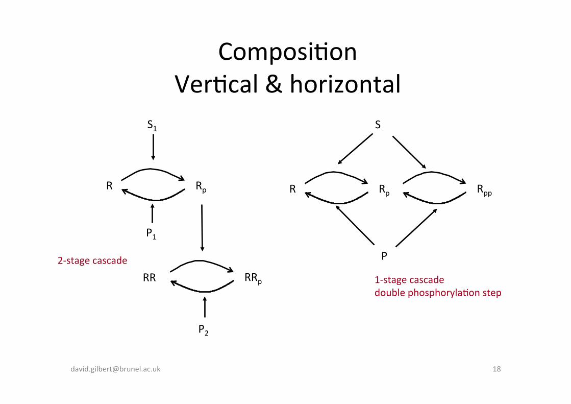
Composi-on Ver-cal & horizontal

Rp R

S1

RRp RR

P1

P2

Rp R

S

Rpp

P 2-‐stage cascade

1-‐stage cascade double phosphoryla-on step


Networks •  Gene regula-on

•  Metabolic

•  Signalling

•  Protein-‐protein interac-on

•  Developmental


What about scaling up?


Mul-scale modelling challenges •  Repe$$on – mul-ple cells witha similar defini-ons

•  Varia$on – mutants.

•  Organisa$on -‐ regular or irregular paterns over spa-al networks in one, two or three dimensions.

•  Communica$on – between neighbours constrained by neighbour rela-on, and the posi-on in spa-al network.

•  Hierarchical organisa$on –cells containing compartments. Enables abstrac-on over level of detail of components.


Mul-scale from signalling to organs

Pam Gao, David Tree

Planar Cell Polarity


Joint work Brunel: •  Pam Gao

•  David Tree

CoObus: •  Monika Heiner

•  Fei Liu


Planar Cell Polarity

A patch of cells (1ssue)

Wing (Organ)

•  Drosophila wing hairs point distally virtually error free. •  Hexagonally packed, planar (300,000) •  PCP: the polariza-on of a field of cells within the plane of a cell sheet. •  Human pathology:

 Cochlear hair cells  Spina bifida  Oncogenic Wnt pathway


Planar Cell Polarity •  The orienta-on of cells within the

plane of the epithelium, orthogonal to the apical-‐basal polarity of the cells.

•  This polarisa-on is required for many developmental events in both vertebrates and non-‐ vertebrates.

•  Defects in PCP in vertebrates underlie developmental abnormali-es in mul-ple -ssues including the neural tube, the kidney and the inner ear


Biological Model •  A core machinery mediates a compe--on between the proximal and distal proteins on adjacent surfaces of neighboring cells and amplifies small differences to result in a highly asymmetric distribu1on of Frizzled (Fz) and Vang. •  As a result of the above machinery, Fz accumulates on the distal side of the cell, designa-ng it as the future site for prehair forma$on, while Vang accumulates on the proximal side of the neighbouring cell. •  There are feedback loops func-oning as well. A consequence of these feedback loops is that cells tent to align their polarity such that each cell accumulates high levels of Fz on the same side of the cell and high levels of Vang on the opposite side.

Symmetric distribu-on of protein complexes

Asymmetric distribu-on of protein complexes

Prehair forma-on [email protected] 27

Biological Model •  An intracellular signalling cascade func-ons downstream of the core machinery, coupling signaling from the core proteins to the cell-‐type specific responses required to generate PCP in the individual -ssues. •  PCP proteins Frizzled (Fz), Dishevelled (Dsh), Prickle (Pk), Flamingo (Fmi) and Van-‐Gogh (Vang)


Biological Model •  At ini-a-on of PCP signalling: Fmi, Fz, Dsh, Vang and Pk are all present symmetrically at

the cell membrane. •  At the conclusion of PCP signalling: Fmi is found at both the proximal and distal cell

membrane, Fz and Dsh are found exclusively at the distal cell membrane and Vang and Pk are found exclusively at the proximal cell membrane.

•  Communica-on between these proteins at cell boundaries. Distally localised Fmi, Fz and Dsh recruit Fmi, Vang and Pk to the proximal cell boundary and vice versa.


ODEs

•  Current model –  Inter-‐cellular signalling: 25 molecular species and 23 reac-ons

–  Kine-c laws: mass ac-on


Parameter Es-ma-on

Simulated Annealing


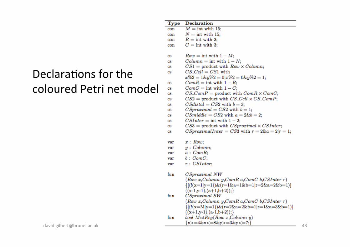
Coloured Petri nets •  Tokens dis-nguished via their colours. •  Each place gets a colour set, specifying the kind of tokens

which can reside on the place. •  Each transi-on gets a guard, specifying which coloured

tokens are required for firing. •  Each arc gets an arc inscrip-on specifying the kind of

tokens flowing through it

•  Allows for the discrimina-on of species (molecules, metabolites, proteins, secondary substances, genes, etc.).

•  Colours can be used to dis-nguish between sub-‐popula-ons of a species in different loca-ons (cytosol, nucleus and so on).


Coloured Petri net •  A coloured Petri net is a tuple N = [P,T,F,Σ,c,g,f,m0], where: •  P is a finite, non-‐empty set of places. •  T is a finite, non-‐empty set of transi-ons. •  F is a finite, non-‐empty set of directed arcs. •  Σ is a finite, non-‐empty set of colour sets. •  c : P → Σ is a colour func-on that assigns to each place p∈P a

colourset c(p)∈Σ. •  g : T → EXP is a guard func-on that assigns to each transi-on t ∈ T

a guard expression of Boolean type. •  f : F → EXP is an arc func-on that assigns to each arc a ∈ F an arc

expression of a mul-set type c(p)MS, where p is the place connected to the arc a.

•  m0 : P → EXP is an ini-alisa-on func-on that assigns to each place p ∈ P an ini-alisa-on expression of a mul-set type c(p)MS.


Coloured Petri net folding


Monika Heiner & Fei Liu

++ mul-set addi-on (+x) successor [x=2] guard

[x=1](x++(+x))++ [x=2]x

Grid constraints (rectangular) neighbour1D(X, A, D1):-‐ (A=X; A = X+1; A = X-‐1), not(A=X), A <= D1, A >= 1. neighbour2D((X,Y), (A,B), (D1,D2)):-‐ (A=X; A = X+1; A = X-‐1), (B=Y; B = Y+1; B = Y-‐1), not((A=X,B=Y)), A <= D1, B <= D2, A >= 1, B >= 1.

neighbour3D((X,Y,Z), (A,B,C), (D1,D2,D3)):-‐ (A=X; A = X+1; A = X-‐1), (B=Y; B = Y+1; B = Y-‐1), (C=Z; C = Z+1; C = Z-‐1), not((A=X,B=Y,C=Z)), A <= D1, B <= D2, C <= D3, A >= 1, B >= 1, C >= 1.


Single cell Abstract level

(Labelled colours not about CPN colour sets)


DBD_left

C

A

E_left

r3

r4

r1

transport proximalcommunication distal

CPN model for cells linked in a pipeline.

C

CS

B

CS

A3

1‘all()CS

D

CSE

CS

r4

r1 r3

x

x

[x>1]−x

x

x

x

x x


colourset CS = int with 1−N, variable x: CS. The arc expression [x > 1]−x indicates that the first cell is not linked to the last.

Spa-al organisa-on & colours

•  Reflect organisa-on by colour structure


(1,1) (1,2) (1,3) (1,4)

(2,1) (2,2) (2,3) (2,4)

(3,1) (3,2) (3,3) (3,4)

(4,1) (4,2) (4,3) (4,4)

Colourset = {(1,1),(1,2),(1,3),(1,4),(2,1),(2,2),(2,3),(2,4), (3,1), (3,2), (3,3), (3,4), (4,1), (4,2), (4,3), (4,4) }

Hierarchical organisa-on

•  Hierarchically coloured


(1,1) (1,2) (1,3) (1,4)

(2,1) (2,2) (2,3) (2,4)

(3,1) (3,2) (3,3) (3,4)

(4,1) (4,2) (4,3) (4,4)

Colourset = {…, {((2,2)(1,1)), ((2,2)(1,2)), ((2,2)(1,3)),……((2,2)(3,3))}, …

(2,2)(1,1) (2,2)(1,2) (2,2)(1,3) (2,2)(2,1) (2,2)(2,2) (2,2)(2,3) (2,2)(3,1) (2,2)(3,2) (2,2)(3,3)

Wing -ssue -ssue: Cells with logical compartments


Petri net model for single cell


CPN model of cells with seven compartments in a 2-‐D matrix.

C CSproximal

E

CSdistal

D

CSdistal

D

CSdistal

B

CSproximal

A

12

1‘all()

CSmiddler1r4 r3NW(x,y,a,b,r) ++

SW(x,y,a,b,r)

((x,y),(a,b))

((x,y),(a,b))

((x,y),(a,b))NW(x,y,a,b,r) ++

SW(x,y,a,b,r)

((x,y),(a,b))

((x,y),(2,2))

((x,y),(2,2))


•  4 spa-al regions: communica-on, proximal, transport and distal

•  Seven virtual compartments ((1, 1), (2, 1),..., (3,3)).

•  Each place or transi-on belongs to a specific compartment.

•  NW and SW denote two leM neighbours of the current cell.

Declara-ons for the coloured Petri net model


CPN model of PCP signalling

FzFmi_FmiVang

CSproximalInter

Fmi_p1‘all()

CSproximal

336

Vang_p

1‘all()

CSproximal

336

FmiVang_p

CSproximal

Pk_p

1‘all()

CSproximal

336

FFDFVP_p

CSproximal

Fz_p

1‘all()

CSproximal

336

Ld_p

1‘all()

CSproximal

336

FFD_p

CSproximal

Dsh_p

1‘all()

CSproximal

336

FzFmi_act_p

CSproximal

FzFmi_pCSproximal

FVP_p

CSproximal

poll2‘all()CSmiddle

224

FFD_dCSdistalFFD_d

CSdistal

Vang_d

1‘all()CSdistal 336

FmiVang_d

CSdistal

Pk_d

1‘all()CSdistal 336

FVP_d

CSdistal

FFDFVP_d

CSdistal

Ld_d

1‘all()

CSdistal

336

Fz_d

1‘all()

CSdistal

336

Fmi_d

1‘all()

CSdistal

336

FzFmi_d

CSdistal

Dsh_d

1‘all()

CSdistal

336

Dsh_d1‘all()

CSdistal

336

FzFmi_act_d

CSdistal

FzFmi_act_d

CSdistal

ri3

[r=2&a=2|r=1]

ri1

[r=2&a=2|r=1]

rp1

rp2

rp5

rp4

rp3

rp9rp8

rp6

rp7

ri2[r=2&a=2|r=1]

rt2

rd11

rd9

rd6

rd7

rd8

rd10

rd1

rd2

rd3

rd5rd4

rt1

rt3

rt6

rt7

rt8rt4

rt9rt5

rt10 P_set1

(((x,y),(a,b)),r)

(((x,y),(a,b)),r)

((x,y),(a,b))

((x,y),(a,b))

((x,y),(a,b))

((x,y),(a,b)) ((x,y),(a,b))

((x,y),(a,b))

((x,y),(a,b))

((x,y),(a,b))

((x,y),(a,b))

((x,y),(a,b))

((x,y),(a,b))

((x,y),(a,b))

((x,y),(a,b))

((x,y),(a,b))

((x,y),(a,b))((x,y),(a,b))((x,y),(a,b))

((x,y),(a,b))

((x,y),(a,b))

((x,y),(a,b))

((x,y),(a,b))

((x,y),(a,b))

((x,y),(a,b))((x,y),(a,b))

((x,y),(a,b))

((x,y),(a,b))

((x,y),(a,b))

((x,y),(a,b))

((x,y),(a,b))

((x,y),(a,b))

((x,y),(a,b))

((x,y),(a,b))

(((x,y),(a,b)),r)

((x,y),(a,b))

((x,y),(1,1))++

((x,y),(2,1))++

((x,y),(3,1))

((x,y),(a,b))

((x,y),(a,b))

((x,y),(a,b))

((x,y),(a,b))

((x,y),(a,b))

((x,y),(a,b))

((x,y),(a,b))

((x,y),(a,b))

((x,y),(a,b))

((x,y),(a,b))

((x,y),(a,b))

((x,y),(a,b))

((x,y),(a,b))

((x,y),(a,b))

((x,y),(a,b))

((x,y),(a,b))

((x,y),(a,b))

((x,y),(a,b)) ((x,y),(a,b))

((x,y),(a,b))

((x,y),(a,b))

((x,y),(a,b))((x,y),(a,b))

((x,y),(a,b))

((x,y),(a,b))

((x,y),(a,b))

((x,y),(a,b))((x,y),(a,b))

((x,y),(a,b))

((x,y),(a,b))

((x,y),(a,b))((x,y),(a,b))

((x,y),(a,b))

((x,y),(1,1))++

((x,y),(2,1))++

((x,y),(3,1))

((x,y),(1,1))++

((x,y),(2,1))++

((x,y),(3,1)) ((x,y),(1,3))++

((x,y),(2,3))++

((x,y),(3,3))

((x,y),(1,3))++

((x,y),(2,3))++

((x,y),(3,3))

((x,y),(1,3))++

((x,y),(2,3))++

((x,y),(3,3))

((x,y),(1,3))++

((x,y),(2,3))++

((x,y),(3,3))

((x,y),(1,1))++

((x,y),(2,1))++

((x,y),(3,1))

((x,y),(1,1))++

((x,y),(2,1))++

((x,y),(3,1))

((x,y),(a,b))

((x,y),(a,b))

((x,y),(1,3))++

((x,y),(2,3))++

((x,y),(3,3))

NW(x,y,a,b,r)++

SW(x,y,a,b,r)

NW(x,y,a,b,r)++

SW(x,y,a,b,r)

NW(x,y,a,b,r)++

SW(x,y,a,b,r)

1((x,y),(2,2))

1

((x,y),(2,2))

1

((x,y),(2,2))1((x,y),(2,2))1((x,y),(2,2))

1

((x,y),(2,2))1((x,y),(2,2)) 1

((x,y),(2,2))

1

((x,y),(2,2))

1

((x,y),(2,2))

Proximal DistalTransportCommunication


FFD in one cell (3,4) Con-nuous simula-on

0

0.1

0.2

0.3

0.4

0.5

0.6

0.7

0.8

0 20 40 60 80 100 120 140 160 180

Con

cent

ratio

n

time

FFD_d_((3,4),(1,3))FFD_d_((3,4),(2,3))FFD_d_((3,4),(3,3))FFD_p_((3,4),(1,3))FFD_p_((3,4),(2,3))FFD_p_((3,4),(3,3))


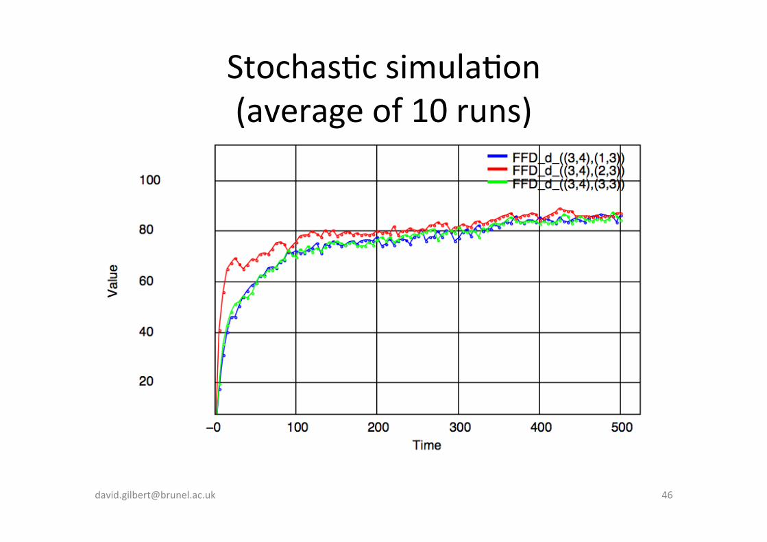
FFD accumulates at the distal edge of the cell rather than the proximal edge at the end of signalling.

Stochas-c simula-on (average of 10 runs)


Some sta-s-cs Size Time (seconds)

Grid(M⇥ N) Cells Places Transitions Unfolding Unfolding/Cells Simulation Simulation/Cells

5⇥ 5 12 924 984 0.99 0.0825 13.34 1.1117

10⇥ 10 50 3,850 4,100 3.46 0.0692 235.81 4.7162

15⇥ 15 112 8,624 9,184 8.04 0.0718 1,366.24 12.1986

20⇥ 20 200 15,400 16,400 15.52 0.0776 - -

50⇥ 50 1,250 96,250 102,500 161.48 0.1292 - -


Size Time (seconds)


5⇥ 5 12 924 984 0.99 0.0825 13.34 1.1117

10⇥ 10 50 3,850 4,100 3.46 0.0692 235.81 4.7162

15⇥ 15 112 8,624 9,184 8.04 0.0718 1,366.24 12.1986

20⇥ 20 200 15,400 16,400 15.52 0.0776 - -

50⇥ 50 1,250 96,250 102,500 161.48 0.1292 - -

Size Time (seconds)


5⇥ 5 12 924 984 0.99 0.0825 13.34 1.1117

10⇥ 10 50 3,850 4,100 3.46 0.0692 235.81 4.7162

15⇥ 15 112 8,624 9,184 8.04 0.0718 1,366.24 12.1986

20⇥ 20 200 15,400 16,400 15.52 0.0776 - -

50⇥ 50 1,250 96,250 102,500 161.48 0.1292 - -

Model Checking Biochemical Pathways

Pathway Model

Property Eg, “Order of peaks is; RafP, MEKPP, ERKPP Model Checker

Yes/no or probability

predicted behaviour

model (knowledge)

observed behaviour

natural biosystem

wetlab experiments

Formalising understanding

model-‐based experiment design

analysis


Simula-on-‐based Model Checking Biochemical Pathways

Model Checker

Model

Property Eg, “Order of peaks is RafP, MEKPP, ERKPP” Yes/no or

probability

Lab Model

Behaviour Checker

Time series data

predicted behaviour

model (blueprint)

observed behaviour

synthe-c biosystem

design construc-on

valida-on

valida-on

desired behaviour

verifica-on


PLTL language •  Behaviours to be checked against a model is expressed in temporal

logic

•  We chose: Probabilis-c logic called Probabilis-c Linear-‐-me Temporal Logic (PLTL)

•  Main PLTL operators: G (P) – P always happens F (P) – P happens at some -me X (P) – P happens in the next -me point (P1) U (P2) – P1 happens un-l P2 happens P1 { P2 } – P1 happens from the first -me P2 happens


Range of expressivity in PLTL •  Qualita1ve:

Protein rises then falls P=? [ ( d(Protein) > 0 ) U ( G( d(Protein) < 0 ) ) ]

•  Semi-‐qualita1ve: Protein rises then falls to less than 50% of peak concentra-on P=? [ ( d(Protein) > 0 ) U ( G( d(Protein) < 0 ) ∧ F ( [Protein] < 0.5 ∗ max[Protein] ) ) ]

•  Semi-‐quan1ta1ve: Protein rises then falls to less than 50% of peak concentra-on by 60 minutes P=? [ ( d(Protein) > 0 ) U ( G( d(Protein) < 0 ) ∧ F ( -me = 60 ∧ Protein < 0.5 ∗ max(Protein) ) ) ]

•  Quan1ta1ve: Protein rises then falls to less than 100µMol by 60 minutes P=? [ ( d(Protein) > 0 ) U ( G( d(Protein) < 0 ) ∧ F ( -me = 60 ∧ Protein < 100 ) ) ]


Model searching Peaks at least once (rises then falls below 50% max concentra-on) P>=1[ ErkPP <= 0.50*max(ErkPP) ∧ d(ErkPP) > 0 U ( ErkPP = max(ErkPP) ∧

F( ErkPP <= 0.50*max(ErkPP) ) ) ]

•  Brown •  Kholodenko •  Schoeberl

Rises and remains constant (99% max concentra-on) P>=1[ErkPP <= 0.50*max(ErkPP) ∧ ( d(ErkPP) > 0 ) U ( G(ErkPP >=

0.99*max(ErkPP)) ) ]

•  Levchenko

Oscillates at least 4 1mes P>=1[ F( d(ErkPP) > 0 ∧ F( d(ErkPP) < 0 ∧ … ) ) ]

•  Kholodenko


Model checking

For each cell (x,y) in the honeycomb: AMer some ini-alisa-on phase, FFD in the middle distal logical compartment (2,3) is always greater than in the other distal compartments (1,3) and (3,3), and will remain so:

P =? [G(-me > init → ([(2,3)] > [(1,3)]&[(3,3)] > [C]))] 15*15 honeycomb grid: 112 cells in total Query holds for all these cells except the cells in the last column,

cells (2,15) to (14,15).


0 50 100 150 200−0.0

0.2

0.4

0.6

0.8

1.0FFD_d_((3,4),(1,3))FFD_d_((3,4),(2,3))FFD_d_((3,4),(3,3))

Continuous Result: continuousCPN_detailedModel_3.colcontped

Time

Valu

e

0 50 100 150 200−0.0

0.2

0.4

0.6

0.8

1.0FFD_d_((2,15),(1,3))FFD_d_((2,15),(2,3))FFD_d_((2,15),(3,3))

Continuous Result: continuousCPN_detailedModel_3.colcontped

Time

Valu

e

Model checking For FFD in each distal compartment of each cell, how many peaks exist in

their traces?

P =?[F ((d[x(2,3)] > 0)&F ((d[x(2,3)] < 0)&F ((d[x(2,3)] > 0))))] P =?[F ((d[x(2,3)] > 0)&F ((d[x(2,3)] < 0)))] P =?[F ((d[x(2,3)] > 0))]

P=?[F( (d[FFD:(3,4),(1,3)] > 0) & F( (d[FFD:(3,4),(1,3)] < 0)))]; Probability: 0.0 P=?[F( (d[FFD:(3,4),(2,3)] > 0) & F( (d[FFD:(3,4),(2,3)] < 0)))]; Probability: 1.0 P=?[F( (d[FFD:(3,4),(3,3)] > 0) & F( (d[FFD:(3,4),(3,3)] < 0)))]; Probability: 0.0

•  No (2,3) peak in cells in Row 1, Row 15 and Column 15 •  Except these boundary cells, other cells have only one peak •  For FFD in other distal compartments, there are no peaks.


Fz clone in WT background


1

Cell position Wild-type Fz- Clone

Row Column Distal Proximal Distal Proximal

3 6 1.72 0.00⇤ 0.37 0.99

4 3 1.72 0.00⇤ 0.37 0.00⇤4 5 2.27 0.00⇤ 0.00 0.00

4 7 1.72 0.00⇤ 0.37 0.99

5 4 2.28 0.00⇤ 0.00 0.00

5 6 2.28 0.00⇤ 0.00 0.00

6 3 1.72 0.00⇤ 0.37 0.00⇤6 5 2.28 0.00⇤ 0.00 0.00

6 7 1.72 0.00⇤ 0.37 1.99

7 4 2.28 0.00⇤ 0.00 0.00

7 6 2.28 0.00⇤ 0.00 0.00

8 3 1.72 0.00⇤ 0.37 0.00⇤8 5 2.28 0.00⇤ 0.00 0.00

8 7 1.72 0.00⇤ 0.37 0.99

9 4 1.72 0.00⇤ 0.37 0.00⇤9 6 1.71 0.00⇤ 0.37 0.99

Acknowledgements Brunel: Pam Gao David Tree

CoObus: Monika Heiner Fei Liu


PhD posi1ons available! [email protected]

biomodelengineering: the...

Documents