biomedical image processing with morphology and …7)/za27227244.pdf · american journal of...

American Journal of Engineering Research (AJER) 2013

w w w . a j e r . o r g

Page 227

American Journal of Engineering Research (AJER)

e-ISSN : 2320-0847 p-ISSN : 2320-0936

Volume-02, Issue-07, pp-227-244

www.ajer.org

Research Paper Open Access

Biomedical Image Processing with Morphology and Segmentation

Methods for Medical Image Analysis

Joyjit Patra1, Himadri Nath Moulick

2, Arun Kanti Manna

3

1(C.S.E, Aryabhatta Institute Of Engineering And Management,Durgapur,West Bengal,India) 2(C.S.E, Aryabhatta Institute Of Engineering And Management,Durgapur,West Bengal,India)

3(C.S.E,Modern Institue Of Engineering & Technology,Bandel,Hoogly,West Best Bengal,India)

Abstract: - Modern three-dimensional (3-D) medical imaging offers the potential and promise for major

advances in science and medicine as higher fidelity images are produced.It has developed into one of the most

important fields within scientific imaging due to the rapid and continuing progress in computerized medical

image visualization and advances in analysis methods and computer-aided diagnosis[1],and is now,for

example,a vital part of the early detection,diagnosis, and treatment of cancer.The challenge is to effectively

process and analyze the images in order to effectively extract, quantify,and interpret this information to gain

understanding and insight into the structure and function of the organs being imaged.The general goal is to

understand the information and put it to practical use.A multitude of diagnostic medical imaging systems are

used to probe the human body.They comprise both microscopic (viz. cellular level) and macroscopic (viz.organ

and systems level) modalities.Interpretation of the resulting images requires sophisticated image processing methods that enhance visual interpretation and image analysis methods that provide automated or semi-

automated tissue detection,measurement, and characterization [2–4].In general,multiple transformations will be

needed in order to extract the data of interest from an image,and a hierarchy in the processing steps will be

evident, e.g., enhancement will precede restoration,which will precede analysis,feature extraction,and

classification[5].Often,these are performed sequentially, but more sophisticated tasks will require feedback of

parameters to preceding steps so that the processing includes a number of iterative loops.Segmentation is one of

the key tools in medical image analysis.The objective of segmentation is to provide reliable, fast, and effective

organ delineation.While traditionally, particularly in computer vision, segmentation is seen as an early vision

tool used for subsequent recognition, in medical imaging the opposite is often true. Recognition can be

performed interactively by clinicians or automatically using robust techniques, while the objective of

segmentation is to precisely delineate contours and surfaces. This can lead to effective techniques known as “intelligent scissors” in 2D and their equivalent in 3D. This paper divided as follows. starts off with a more

“philosophical” section setting the background for this study. We argue for a segmentation context where high-

level knowledge, object information, and segmentation method are all separate. we survey in some detail a

number of segmentation methods that are well-suited to image analysis, in particular of medical images.We

illustrate this, make some comparisons and some recommendations. we introduce very recent methods that unify

many popular discrete segmentation methods and we introduce a new technique. we give some remarks about

recent advances in seeded, globally optimal active contour methods that are of interest for this study. we

compare all presented methods qualitatively. We then conclude and give some indications for future work.

Nonlinear filtering techniques are becoming increasingly important in image processing applications, and are

often better than linear filters at removing noise without distorting image features. However, design and

analysis of nonlinear filters are much more difficult than for linear filters. One structure for designing nonlinear

filters is mathematical morphology, which creates filters based on shape and size characteristics. Morphological filters are limited to minimum and maximum operations that introduce bias into images. This

precludes the use of morphological filters in applications where accurate estimation of the true gray level is

necessary.

This work develops two new filtering structures based on mathematical morphology that overcome the

limitations of morphological filters while retaining their emphasis on shape. The linear combinations of

morphological filters eliminate the bias of the standard filters, while the value-and-criterion filters allow a



28

variety of linear and nonlinear operations to be used in the geometric structure of morphology. One important

value-and-criterion filter is the Mean of Least Variance (MLV) filter, which sharpens edges and provides noise

smoothing equivalent to linear filtering. To help understand the behavior of the new filters, the deterministic

and statistical properties of the filters are derived and compared to the properties of the standard

morphological filters. In addition, new analysis techniques for nonlinear filters are introduced that describe the

behavior of filters in the presence of rapidly fluctuating signals, impulsive noise, and corners. The corner

response analysis is especially informative because it quantifies the degree to which a filter preserves corners of all angles.Examples of the new nonlinear filtering techniques are given for a variety of medical images,

including thermographic, magnetic resonance, and ultrasound images. The results of the filter analyses are

important in deciding which filter to use for a particular application. For thermography, accurate gray level

estimation is required, so linear combinations of morphological operators are appropriate. In magnetic

resonance imaging (MRI), noise reduction and contrast enhancement are desired. The MLV filter performs

these tasks well on MR images. The new filters perform as well or better than previously established techniques

for biomedical image enhancement in these applications.

Keywords: - Spatial Filter, Image Denoising, Median Filter, Midrange Filter, Pseudomedian Filter, Random

Walkers.

I. INTRODUCTION

The major strength in the application of computers to medical imaging lies in the use of image

processing techniques for quantitative analysis. Medical images are primarily visual in nature; however, visual

analysis by human observers is usually associated with limitations caused by interobserver variations and errors due to

fatigue, distractions, and limited experience. While the interpretation of an image by an expert draws

from his/her experience and expertise, there is almost always a subjective element. Computer analysis, if

performed with the appropriate care and logic, can potentially add objective strength to the interpretation of the

expert. Thus,it becomes possible to improve the diagnostic accuracy and confidence of even an expert with

many years of experience.Imaging science has expanded primarily along three distinct but related lines of

investigation: segmentation, registration and visualization [6]. Segmentation, particularly in three dimensions,

remains the holy grail of imaging science. It is the important yet elusive capability to accurately recognize and

delineate all the individual objects in an image scene. Registration involves finding the transformation that

brings different images of the same object into strict spatial (and/or temporal) congruence.And visualization

involves the display, manipulation, and measurement of image data. A common theme throughout this book is

the differentiation and integration of images. On the one hand, automatic segmentation and classification of tissues provide the required differentiation, and on the other the fusion of complementary images provides the

integration required to advance our understanding of life processes and disease. Measurement of both form and

function, of the whole image and at the individual pixel level, and the ways to display and manipulate digital

images are the keys to extracting the clinical information contained in biomedical images.The need for new

techniques becomes more pressing as improvements in imaging technologies enable more complex objects to be

imaged and simulated.

The approach required is primarily that of problem solving. However, the understanding of the problem

can often require a significant amount of preparatory work.The applications chosen for this book are typical of

those in medical imaging; they are meant to be exemplary, not exclusive. Indeed, it is hoped that many of the

solutions presented will be transferable to other problems. Each application begins with a statement of the

problem, and includes illustrations with real-life images. Image processing techniques are presented, starting with relatively simple genericmethods, followed bymore sophisticated approaches directed at that specific

problem.The benefits and challenges in the transition from research to clinical solution are also

addressed.Biomedical imaging is primarily an applied science, where the principles of imaging science are

applied to diagnose and treat disease, and to gain basic insights into the processes of life.The development of

such capabilities in the research.laboratory is a time-honored tradition. The challenge is to make new techniques

available outside the specific laboratory that developed them, so that others can use and adapt them to different

applications. The ideas, skills and talents of specific developers can then be shared with a wider community and

this will hopefully facilitate the transition of successful research technique into routine clinical use.Nonlinear

methods in signal and image processing have become increasingly popular over the past thirty years.There are

two general families of nonlinear filters: the homomorphic and polynomial filters, and the order statistic and

morphological filters [1]. Homomorphic filters were developed during the 1970's and obey a generalization of

the superposition principle [2]. The polynomial filters are based on traditional nonlinear system theory and use Volterra series. Analysis and design of homomorphic and polynomial filters resemble traditional methods used



Page 229

for linear systems and filters in many ways.The order statistic and morphological filters, on the other hand,

cannot be analyzed efficiently using generalizations of linear techniques.The median filter is an example of an

order statistic filter, and is probably the oldest [3, 4] and most widely used order statistic filter. Morphological

filters are based on a form of set algebra known as mathematical morphology. Most morphological filters use

extreme order statistics (minimum and maximum values) within a filter window, so they are closely related to

order statistic filters [5, 6].While homomorphic and polynomial filters are designed and analyzed by the

techniques used to define them, order statistic filters are often chosen by more heuristic methods. As a result, the behavior of the median filter and other related filters was poorly understood for many years. In the early 1980's,

important results on the statistical behavior of the median filter were presented [7], and a new technique was

developed that defined the class of signals invariant to median filtering, the root signals [8, 9]. Morphological

filters are derived from a more rigorous mathematical background [10-12], which provides an excellent basis for

design but few tools for analysis. Statistical and deterministic analyses for the basic morphological filters were

not published until 1987 [5, 6, 13].The understanding of the filters’ behavior achieved by these analyses is not

complete, however, so further study may help determine when morphological filters are best applied.

II. MEDIAN FILTER ROOT SIGNALS

The median filter is an order statistic (stack) filter that replaces the center value in the filter window

with the median of the values in the window. If the values in the window are updated as the filter acts on the

signal, it is called a recursive median filter. Non-recursive median filtering, which is far more common than

recursive median filtering, always acts on the original values in the signal. For a signal f(x) and a filter window

W, the non-recursive median filter is denoted as shown in equation (1) below:

..................(1)

Repeated application of the median filter is denoted by a superscript; for example, med3(f; W) denotes the result of three iterations of the non-recursive median filter with window W over the signal f. The root signal

set of the 1-D median filter for finite-length signals consists only of signals that are everywhere locally

monotonic of length n + 2, where W is 2n+1 points long W = 2n(+1)[8, 9]. This means that any section of a

finite-length median root signal of at least n + 2 points is monotonic (nonincreasing or nondecreasing). This

result assumes the signal is padded appropriately with constant regions to obtain the filter output near the ends,

as described previously. Gallagher and Wise [9] stated the same result slightly differently: a finite-length

median root signal consists only of constant neighborhoods and edges. A constant neighborhood is an area of

constant value of at least length n + 1 (just over half the length of W) and an edge is a monotonic region of any

length between two constant neighborhoods.This root signal set indicates that the median filter preserves slowly

varying regions and sharp edges, but alters impulses and rapid oscillations. For infinite-length signals, Tyan [8]

showed that another type of root signal exists for the non-recursive median filter. These root signals, the ―fastfluctuating‖ roots, consist solely of rapid oscillations between two values. Nowhere in these signals is there

even one monotonic region of length n + 1. For example, the infinite-length signal ..., 1, 0, 1, 0, 1, 0, 1, 0, ... is a

root of the nonrecursive median filter with a window width of 4k+1, where k is any positive integer. Although

this type of signal is seldom encountered in practical applications, sections of a finite-length signal that fluctuate

quickly (even if they are not bi-valued) are often passed by the median filter without much smoothing. An

example of this situation is shown in Figure 1. The original signal has an oscillation in it, and when filtered by a

5-wide median filter only the first and last two peaks in the oscillation are smoothed.

Figure 1. Oscillatory signal filtered by a 5-wide non-recursive median filter.



Page 230

Gallagher and Wise [9] showed that repeated iteration of the non-recursive median filter on a signal of

length L reduces the signal to a root signal in at most (L–2)/2 passes. This result comes from the observation that

on the first pass, the first and last values must be unchanged; on succeeding passes, the area at the beginning and

end of the signal that is unchanged by filtering is at least one point longer. Figure 1 also illustrates how

oscillatory signals are reduced to a root a few points at a time from either end. The root signal resulting from

repeated iteration of the non-recursive median filter is denoted med∞(f; W). Although the number of passes

required to reduce most signals to a median root is fairly small, in some instances the number of passes required is very large.The recursive median filter yields a root signal from any input signal in a single pass; however, the

resulting root is usually not as good a representation of the original signal as med∞(f; W). This is because the

recursive filter allows signal values to propagate along the signal sequence, so that the output value at any point

is not necessarily related to the values currently in the filter window.The recursive median filter is rarely used in

practice for this reason. Figure 2 is an example of 5-wide recursive median filtering on the same signal as in

Figure1. The result is a root signal, but it is very different from the result of nonrecursive median filtering.

Figure 2. Oscillatory signal filtered by a 5-wide recursive median filter.

III. INEAR COMBINATIONS OF MORPHOLOGICAL OPERATORS

Since the complementary morphological operators (OC and CO; opening and closing; erosion and

dilation) are equally and oppositely biased, an obvious way to try to remove the bias is by simply taking the

average of the two operators. For symmetric input noise distributions, an evenly weighted average clearly

should give an unbiased result; however, for asymmetric distributions an unequally weighted average of the two

operators may work better for removing the bias.This chapter describes the various types of linear combinations

of morphological operators and illustrates how they alleviate some of the bias problems of standard

morphological filters. Theorems describing the root signal sets of these linear combinations are presented, and

approximations for the statistical properties of the filters are also given and compared to the properties of the

standard morphological filters.

Midrange Filter

The midrange filter is defined as the average of the maximum and the minimum values in a filter window, the midpoint of the range of values in the window. Since the erosion is a sliding minimum operation acting over the

window N and dilation is a sliding maximum operation acting over the same window, another form of the

midrange filter is the average of the two basic morphological operators, erosion and dilation. The midrange filter

is a wellknown estimator in the order statistics literature; see, for example, [25-27]. The midrange filter is

optimal in the mean square sense among all filters that are linear combinations of order statistics for removing

uniformly distributed noise from a constant signal [26]. The midrange filter is also the maximum likelihood

estimator for uniformly distributed noise [26].The notation for the midrange filter is given in equation (9) below.

…………(2)



Page 231

Pseudomedian Filter

The pseudomedian filter was originally defined in 1985 by Pratt, Cooper, and Kabir [28]. They defined

the filter in one dimension to be the average of the maximum of the minima of n+1 subwindows within an

overall window and the minimum of the maxima of the same subwindows. Each subwindow is n+1 points long,

and is within an overall window of length 2n+1. This structure corresponds to that of morphological opening

and closing: the subwindows are the structuring elements N, and the overall window is W. Pratt recast the

definition of the pseudomedian filter in his 1991 text [29] by forming the ―maximin‖ and ―minimax‖ functions, which he averages to find the pseudomedian. The maximin and minimax functions are equivalent to

morphological opening and closing. The 1-D pseudomedian filter is therefore the average of the opening and

closing, as noted previously by this author [30]. Pratt defined a two-dimensional pseudomedian filter in a

manner that does not correspond to 2-D opening and closing; however, other work by the author [31, 32]

generalized the pseudomedian filter to two dimensions in a manner corresponding to the definition of the

pseudomedian as the average of opening and closing. The notation for pseudomedian filter is given in equation

(10)

below.

…………..(3)

Pseudomedian Filter

The deterministic behavior of the pseudomedian filter is quite different from that of the midrange filter.

Theorem 3.15 below proves that the root signal set of the pseudomedian filter for bounded signals includes only

signals that consist entirely of constant neighborhoods and edges.

Theorem 3.15: A bounded root signal of the pseudomedian filter consists only of constant neighborhoods and edges.

Proof: Suppose f(x) is a root signal of the pseudomedian filter with structuring element N of length |N| = n+1;

that is, f(x) = pmed(f(x); N).

This proof will proceed by defining three possible cases for the root signals. The opening and closing of the

signal may be equal at all points, or may be unequal at all points, or may be equal at some points and unequal at

others. The case where opening and closing are equal at all points corresponds to the root signals consisting of

constant neighborhoods and edges. The other two cases show that there are not roots where the opening and

closing are unequal at all points or where opening and closing are equal at some points and unequal at other

points.

Together, the definition of the pseudomedian filter and the above assumption imply that

for all x.

f(x) of the pseudomedian filter is everywhere LOMO(n+2); that is, f(x) consists only of constant neighborhoods

and edges. Case II: fN(x) ≠f N(x) for all x.

First, assume that there exists a point x1 such that . By Theorem 6, fN(x1) = f(x1).

Then, by the definition of the pseudomedian filter, fN(x1) = f N(x1), which is a contradiction. Similarly, if there

is a point x2 such that then f N(x2) = f(x2). Again, fN(x2) = f N(x2), which is a contradiction. Therefore, for Case II there can be no point x where f(x) is equal to the erosion, dilation, opening,

or closing at x. fN(x) and f N(x) are then infinitely long and n-monotonic everywhere.f N(x) ≥ fN(x), so the

closing and opening must be both increasing or both decreasing, since any infinite n-monotonic increasing

signal must be greater than any infinite n-monotonic decreasing signal as x+∞and less than any infinite n-

monotonic decreasing signal as x–∞.The average of two signals that are n-monotonic and either both increasing or both decreasing is a signal that is n-monotonic. Therefore, the pseudomedian of a signal f(x) that

satisfies fN(x)≠f N(x) for all x is an nmonotonic signal. However, if f(x) is n-monotonic, then fN(x) = f(x) = f

N(x), which is a contradiction of fN(x)≠f N(x). Therefore, there exist no root signals of the pseudomedian filter

that satisfy Case II.



Page 232

Seed-Driven Segmentation

Segmentation is a fundamental operation in computer vision and image analysis. It consists of

identifying regions of interests in images that are semantically consistent.Practically, this may mean finding

individual white blood cells amongst red blood cells; identifying tumors in lungs; computing the 4D hyper-

surface of a beating heart, and so on. Applications of segmentation methods are numerous. Being able to

reliably and readily characterize organs and objects allows practitioners to measure them, count them and

identify them. Many images analysis problems begin by a segmentation step, and so this step conditions the quality of the end results. Speed and ease of use are essential to clinical practice. This has been known for quite

some time, and so numerous segmentation methods have been proposed in the literature [57]. However,

segmentation is a difficult problem. It usually requires high-level knowledge about the objects under study. In

fact, semantically consistent, high-quality segmentation, in general, is a problem that is indistinguishable from

strong Artificial Intelligence and has probably no exact or even generally agreeable solution. In medical

imaging, experts often disagree amongst themselves on the placement of the 2D contours of normal organs, not

to mention lesions. In 3D, obtaining expert opinion is typically difficult, and almost impossible if the object

under study is thin, noisy and convoluted, such as in the case of vascular systems. At any rate, segmentation is,

even for humans, a difficult, time-consuming and error-prone procedure.

Image Analysis and Computer Vision

Segmentation can be studied from many angles. In computer vision, the segmentation task is often seen as a low-level operation, which consists of separating an arbitrary scene into reasonably alike components (such

as regions that are consistent in terms of color, texture and so on). The task of grouping such component into

semantic objects is considered a different task altogether. In contrast, in image analysis, segmentation is a high-

level task that embeds high-level knowledge about the object. This methodological difference is due to the

application field. In computer vision, the objective of segmentation (and grouping) is to recognize objects in an

arbitrary scene, such as persons, walls, doors, sky, etc. This is obviously extremely difficult for a computer,

because of the generality of the context, although humans do generally manage it quite well. In contrast, in

image analysis, the task is often to precisely delineate some objects sought in a particular setting known in

advance. It might be for instance to find the contours of lungs in an X-ray photograph. The segmentation task in

image analysis is still a difficult problem, but not to the same extent as in the general vision case. In contrast to

the vision case, experts might agree that a lesion is present on a person’s skin, but may disagree on its exact contours [45]. Here, the problem is that the boundary between normal skin and lesion might be objectively

difficult to specify. In addition, sometimes there does exist an object with a definite physical contour (such as

the inner volume of the left ventricle of the heart). However, imaging modalities may be corrupted by noise and

partial volume effects to an extent that delineating the precise contours of this physical object in an image is also

objectively difficult.

Objects Are Semantically Consistent

However, in spite of these difficulty, we may assume that, up to some level of ambiguity, an object

(organ, lesion, etc) may still be specified somehow. This means that semantically, an object possess some

consistency.When we point at a particular area on an image, we expect to be, again with some fuzziness, either

inside or outside the object This leads us to the realize that there must exist some mathematical indicator

function, that denotes whether we are inside or outside of the object with high probability. This indicator function can be considered like a series of constraints, or labels. They are sometimes called seeds or markers, as

they provide starting points for segmentation procedures, and they mark where objects are and are not. In

addition, a metric that expresses the consistency of the object is likely to exist. A gradient on this metric may

therefore provide object contour information. Contours may be weak in places where there is some uncertainty,

but we assume they are not weak everywhere (else we have an ambiguity problem, and our segmentation cannot

be precise). The metric may simply be the image intensity or color, but it may express other information like

consistency of texture for instance. Even though this metric may contain many descriptive elements (as a vector

of descriptors for instance), we assume that we are still able to compute a gradient on this metric [61]. This is

the reason why many segmentation methods focus on contours, which are essentially discontinuities in the

metric. Those that focus on regions do so by defining and utilizing some consistency metric, which is the same

problem expressed differently. The next and final step for segmentation is the actual contour placement, which is equivalent to object delineation. This step can be considered as an optimization problem, and this is the step

on which segmentation methods in the literature focus the most. We will say more about this in Sect. 3.2 listing

some image segmentation categories.



Page 233

Desirable Properties of Seeded Segmentation Methods

We come to the first conclusion that to provide reliable and accurate results, we must rely on a

segmentation procedure and not just an operator. Object identification and constraints analysis will set us in

good stead to achieve our results, but not all segmentation operators are equivalent.We can list here some

desirable properties of interactive segmentation operators. • It is useful if the operator can be expressed in an

energy or cost optimization formulation. It is then amenable to existing optimizationmethods, and this entails a

number of benefits. Lowering the cost or the energy of the formulation can be done in several ways (e.g. continuous or discrete optimization), which results in different characteristics and compromises, say between

memory resources and time. Optimizationmethods improve all the time through the work of researchers,and so

our formulations will benefit too.

• It is desirable if the optimization formulation can provide a solution that is at least locally optimal, and if

possible globally optimal, otherwise noise will almost certainly corrupt the result.

• The operator should be fast, and provide guaranteed convergence, because it will be most likely restarted

several times, in order to adjust parameters. Together with this requirement, the ability to segment many objects

at once is also desirable, otherwise the operator will need to be restarted as many time as there are objects in the

image. This may not be a big problem if objects do not overlap and if bounding boxes can be drawn around

them, because the operator can then be run only within the bounding box, but this is not the general case.

• The operator should be bias-free: e.g. with respect to objects size or to the discretization grid or with respect to

initialization. • The operator should be flexible: it is useful if it can be coupled with topology information for instance, or with

multi-scale information.

• It should be generic, not tied to particular data or image types.

• It should be easy to use. This in practice means possessing as few parameters as possible. Of course one can

view constraints setting as an enormous parameter list, but this is the reason why we consider this step as

separate. Such a method certainly does not yet exist to our knowledge, although some might be considered to

come close. We describe some of them in the next section.

Pixel Selection

Pixel selection is likely the oldest segmentation method. It consists of selecting pixels solely based on

their values and irrespective of their spatial neighborhood. The simplest pixel selection method is humble thresholding, where we select pixels that have a gray-level value greater or smaller than some threshold value.

This particular method is of course very crude, but is used frequently nonetheless. Multiple thresholding uses

several values instead of a single value; color and multispectral thresholding using vectors of values and not just

scalars. By definition all histogram-based methods for finding the parameters of the thresholding, including

those that optimize a metric to achieve this [54], are pixel selection methods.Statistical methods (e.g. spectral

classification methods) that include no spatial regularization fall into this category as well. This is therefore a

veritable plethora of methods that we are including here, and research is still active in this domain. Of course,

thresholding and related methods are usually very fast and easily made interactive, which is why they are still

used so much. By properly pre-processing noisy, unevenly illuminated images, or by other transforms, it is

surprising how many problems can be solved by interactive or automated thresholding. However, this is of

course not always the case, hence the need for more sophisticated methods.

Contour Tracking

It was realized early on that (1) human vision is sensitive to contours and (2) there is a duality between

simple closed contours and objects. A simple closed contour (or surface) is one that is closed and does not self-

intersect. By the Jordan theorem, in the Euclidean space, any such contour or surface delineates a single object

of finite extent. There are some classical difficulties with the Jordan theorem in the discrete setting [52], but

they can be solved by selecting proper object/background connectivities, or by using a suitable graph, for

instance, the 6-connected hexagonal grid or the Khalimsky topology [22, 40]. A contour can be defined locally

(it is a frontier separating two objects (or an object and its background in the binary case)), while an object

usually cannot (an object can have an arbitrary extent). A gradient (first derivative) or a Laplacian (second

derivative) operator can be used to define an object border in many cases, and gradients are less sensitive to

illumination conditions than pixel values. As a result, contour detection through the use of gradient or Laplacian operators became popular, and eventually led to the Marr–Hildreth theory [44]. Given this, it is only natural that

most segmentation method use contour information directly in some ways, and we will revisit this shortly. Early

methods used only this information to detect contours and then tried to combine them in some way. By far the

most popular and successful version of this approach is the Canny edge detector [9]. In his classical paper,

Canny proposed a closed-form optimal 1D edge detector assuming the presence of additive white Gaussian



Page 234

noise, and successfully proposed a 2D extension involving edge tracking using non-maxima suppression with

hysteresis.One problem with this approach is that there is no optimality condition in 2D, no topology or

connectivity constraints and no way to impose markers in the final result. All we get is a series of contours,

which may or may not be helpful. Finding a suitable combination of detected contours (which can be

incomplete) to define objects is then a combinatorial problem of high complexity. Finally, this approach extends

even less to 3D.Overall, in practical terms, these contour tracking methods have been superseded by more recent

methods and should not be used without good reasons. For instance, more recent minimal-path methods can be applied to contour tracking methods, although they are much more sophisticated in principle [3, 14]. In this class

of methods belongs also the ―intelligent scissors‖ types. There were many attempts in previous decades to

provide automated delineating tools in various image processing software packages, but a useful contribution

was provided relatively recently by Mortensen [48]. This method is strictly interactive, in the sense that it is

designed for human interaction and feedback. ―Intelligent scissor‖ methods are useful to clinicians for providing

ground truth data for instance. Such methods are still strictly 2D. As far as we know, no really satisfying 3D

live-wire/intelligent scissor method is in broad use today [5]. However, minimal surfaces methods, which we

will describe, in some ways do perform this extension to nD [30].

Continuous Optimization Methods

In the late 1980s, it was realized that contour tracking methods were too limited for practical use.

Indeed, getting closed contours around objects were difficult to obtain with contour tracking. This meant that detecting actual objects was difficult except in the simplest cases.

Active Contours

Researchers, therefore, proposed to start from already-closed loops, and to make them evolve in such a

way that they would converge towards the true contours of the image. Thus were introduced active contours, or

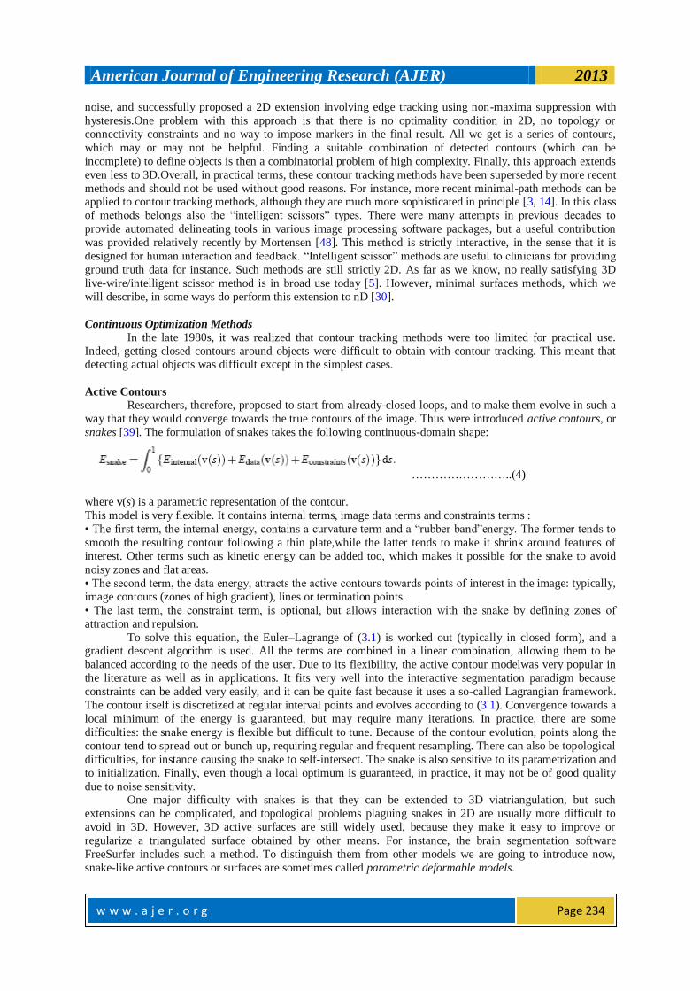
snakes [39]. The formulation of snakes takes the following continuous-domain shape:

……………………..(4)

where v(s) is a parametric representation of the contour.

This model is very flexible. It contains internal terms, image data terms and constraints terms :

• The first term, the internal energy, contains a curvature term and a ―rubber band‖energy. The former tends to

smooth the resulting contour following a thin plate,while the latter tends to make it shrink around features of

interest. Other terms such as kinetic energy can be added too, which makes it possible for the snake to avoid

noisy zones and flat areas.

• The second term, the data energy, attracts the active contours towards points of interest in the image: typically,

image contours (zones of high gradient), lines or termination points.

• The last term, the constraint term, is optional, but allows interaction with the snake by defining zones of

attraction and repulsion.

To solve this equation, the Euler–Lagrange of (3.1) is worked out (typically in closed form), and a gradient descent algorithm is used. All the terms are combined in a linear combination, allowing them to be

balanced according to the needs of the user. Due to its flexibility, the active contour modelwas very popular in

the literature as well as in applications. It fits very well into the interactive segmentation paradigm because

constraints can be added very easily, and it can be quite fast because it uses a so-called Lagrangian framework.

The contour itself is discretized at regular interval points and evolves according to (3.1). Convergence towards a

local minimum of the energy is guaranteed, but may require many iterations. In practice, there are some

difficulties: the snake energy is flexible but difficult to tune. Because of the contour evolution, points along the

contour tend to spread out or bunch up, requiring regular and frequent resampling. There can also be topological

difficulties, for instance causing the snake to self-intersect. The snake is also sensitive to its parametrization and

to initialization. Finally, even though a local optimum is guaranteed, in practice, it may not be of good quality

due to noise sensitivity. One major difficulty with snakes is that they can be extended to 3D viatriangulation, but such

extensions can be complicated, and topological problems plaguing snakes in 2D are usually more difficult to

avoid in 3D. However, 3D active surfaces are still widely used, because they make it easy to improve or

regularize a triangulated surface obtained by other means. For instance, the brain segmentation software

FreeSurfer includes such a method. To distinguish them from other models we are going to introduce now,

snake-like active contours or surfaces are sometimes called parametric deformable models.



Page 235

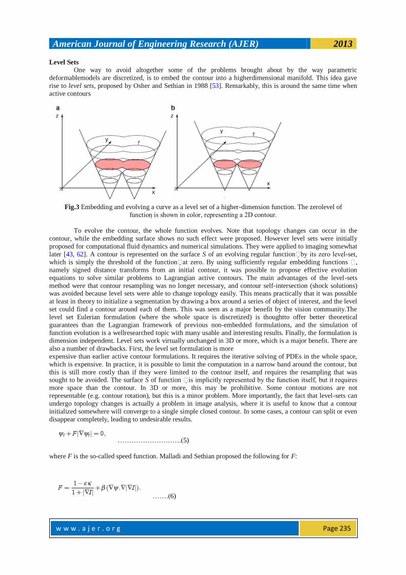
Level Sets

One way to avoid altogether some of the problems brought about by the way parametric

deformablemodels are discretized, is to embed the contour into a higherdimensional manifold. This idea gave

rise to level sets, proposed by Osher and Sethian in 1988 [53]. Remarkably, this is around the same time when

active contours

Fig.3 Embedding and evolving a curve as a level set of a higher-dimension function. The zerolevel of

function is shown in color, representing a 2D contour.

To evolve the contour, the whole function evolves. Note that topology changes can occur in the

contour, while the embedding surface shows no such effect were proposed. However level sets were initially

proposed for computational fluid dynamics and numerical simulations. They were applied to imaging somewhat

later [43, 62]. A contour is represented on the surface S of an evolving regular functionby its zero level-set,

which is simply the threshold of the functionat zero. By using sufficiently regular embedding functions ,

namely signed distance transforms from an initial contour, it was possible to propose effective evolution

equations to solve similar problems to Lagrangian active contours. The main advantages of the level-sets

method were that contour resampling was no longer necessary, and contour self-intersection (shock solutions) was avoided because level sets were able to change topology easily. This means practically that it was possible

at least in theory to initialize a segmentation by drawing a box around a series of object of interest, and the level

set could find a contour around each of them. This was seen as a major benefit by the vision community.The

level set Eulerian formulation (where the whole space is discretized) is thoughtto offer better theoretical

guarantees than the Lagrangian framework of previous non-embedded formulations, and the simulation of

function evolution is a wellresearched topic with many usable and interesting results. Finally, the formulation is

dimension independent. Level sets work virtually unchanged in 3D or more, which is a major benefit. There are

also a number of drawbacks. First, the level set formulation is more

expensive than earlier active contour formulations. It requires the iterative solving of PDEs in the whole space,

which is expensive. In practice, it is possible to limit the computation in a narrow band around the contour, but

this is still more costly than if they were limited to the contour itself, and requires the resampling that was sought to be avoided. The surface S of function is implicitly represented by the function itself, but it requires

more space than the contour. In 3D or more, this may be prohibitive. Some contour motions are not

representable (e.g. contour rotation), but this is a minor problem. More importantly, the fact that level-sets can

undergo topology changes is actually a problem in image analysis, where it is useful to know that a contour

initialized somewhere will converge to a single simple closed contour. In some cases, a contour can split or even

disappear completely, leading to undesirable results.

……………………….(5)

where F is the so-called speed function. Malladi and Sethian proposed the following for F:

…….(6)



Page 236

The first part of the equation is a term driving the embedding function towards contours of the

image with some regularity and smoothing controlled by the curvature . The amount of smoothing is

controlled by the parameter ∑. The second term is a ―balloon‖ force that tends to expand the contour. It is

expected that the contour initially be placed inside the object of interest, and that this balloon force should be

reduced or eliminated after some iterations, controlled by the parameter .We see here that even though this model is relatively simple for a level-set one, it already has a few parameters that are not obvious to set or

optimize.

Geodesic Active Contours An interesting attempt to solve some of the problems posed by overly general level sets was to go back

and simplify the problem, arguing for consistency and a geometric interpretation of the contour obtained. The

result was the geodesic active contour (GAC), proposed by Caselles et al. in 1997 [10]. The level set

formulation is the following:

…….(7)

This equation is virtually parameter-free, with only a g function required. This function is a metric and

has a simple interpretation: it defines at point x the cost of a contour going through x. This metric is expected to be positive definite, and in most cases is set to be a scalar functional with values in R+. In other words, the

GAC equation finds the solution of:

……(8)

where C is a closed contour or surface. This is the minimal closed path or minimal closed surface

problem, i.e. finding the closed contour (or surface) with minimum weight defined by g. In addition to

simplified understanding and improved consistency, (3.4) has the required form for Weickert’s PDE operator splitting [28, 68],allowed PDEs to be solved using separated semi-implicit schemes for improved efficiency.

These advances made GAC a reference method for segmentation, which is now widely used and implemented in

many software packages such as ITK. The GAC is an important interactive segmentation method due to the

importance of initial contour placement, as with all level-sets methods. Constraints such as forbidden or

attracting zones can all be set through the control of function g, which has an easy interpretation. As an

example, to attract the GAC towards zones of actual image contours, we could set

……..(9)

With p = 1 or 2. We see that for this function, g is small (costs little) for zones where the gradient is

high. Many other functions, monotonically decreasing for increasing values for can be used instead. One

point to note, is that GAC has a so-called shrinking bias, due to the fact that the globally optimal solution for (3.5) is simply the null contour (the energy is then zero). In practice, this can be avoided with balloon forces but

the model is again non-geometric. Because GAC can only find a local optimum, this is not a serious problem,

but this does mean that contours are biased towards smaller solutions.

RandomWalkers

In order to correct some of the problems inherent to graph cuts, Grady introduced the RandomWalker

(RW) in 2004 [29,32].We set ourselves in the same framework as in the Graph Cuts case with a weighted graph,

but we consider from the start a multilabel problem, and, without loss of generality, we assume that the

edgeweights are all normalized between 0 and 1. This way, they represent the probability that a random particle

may cross a particular edge to move from a vertex to a neighboring one. Given a set of starting points on this

graph for each label, the algorithm considers the probability for a particle moving freely and randomly on this

weighted graph to reach any arbitrary unlabelled vertex in the graph before any other coming from the other



Page 237

labels. A vector of probabilities, one for each label, is therefore computed at each unlabeled vertex. The

algorithm considers the computed probabilities at each vertex and assigns the label of the highest probability to

that vertex. Intuitively, if close to a label starting point the edge weights are close to 1, then its corresponding

―random walker‖ will indeed walk around freely, and the probability to encounter it will be high. So the label is

likely to spread unless some other labels are nearby. Conversely, if somewhere edge weights are low, then the

RW will have trouble crossing these edges. To relate these observations to segmentation, let us assume that edge

weights are high within objects and low near edge boundaries. Furthermore, suppose that a label starting point is set within an object of interest while some other labels are set outside of it. In this situation, the RW is likely to

assign the same label to the entire object and no further, because it spreads quickly within the object but is

essentially stopped a the boundary. Conversely, the RW spreads the other labels outside the object, which are

also stopped at the boundary. Eventually, the whole image is labeled with the object of interest consistently

labeled with a single value.

Watershed

While there are many variations on discrete segmentationmethods, we will consider one last method:

the Watershed Transform (WT). It was introduced in 1979 by Beucher and Lantu´ejoul [6] by analogy to the

topography feature in geography. It can be explained intuitively in the following manner: consider a gray-level

image to be a 3D topographical surface or terrain. A drop of water falling onto this surface would follow a

descending path towards a local minimum of the terrain.The set of points, such that drops falling onto them would flow into the same minimum, is called a catchment basin. The set of points that separate catchment

basins form the watershed line. Finally, the transform that takes an image as input and produces its set of

watershed lines is called the Watershed Transform. To use

Fig. 4 Watershed segmentation: (a) anMRI image of the heart, (b) its smoothed gradient, (c) the gradient seen as

a topographic surface, (d) Watershed of the gradient, and (e) topographical view of the watershed

this transform in practical segmentation settings, we must reverse the point of view somewhat. Assume

now that labels are represented by lakes on this terrain and that by some flooding process, the water level rises

evenly. The set of points that are such that waters from different lakes meet is also called the watershed line.

Now this watershed line is more constrained, because there are only as many lines as necessary to separate all

the lakes. This intuitive presentation is useful but does not explain why theWT is useful for segmentation. As

the ―terrain‖, it is useful to consider the magnitude of the gradient of the image. On this gradient image, interior

objects will have values close to zero and will be surrounded by zones of high values: the contours of the

objects. They can therefore be assimilated to catchment basins, and the WT can delineate them well (see Fig. 4).The WT is a seeded segmentation method, and has many interesting interpretations.If we consider the image

again as a graph as in the GC setting, then on this graph the set of watershed lines from the WT form a graph

cut. The edges of this tree can be weighted with a functional derived from a gradient exactly as in the GC case.

Computing the WT can be performed in many efficient ways [46, 67], but an interesting one is to consider the

Maximum Spanning Forest (MSF) algorithm [19]. In this algorithm, the classical graph algorithm for maximum



Page 238

spanning tree (MST) is run on the graph of the image, following for instance Kruskal’s algorithm [41,59], with

the following difference: when an edge selected by the MST algorithm is connected with a seed, then all vertices

that are connected with it become also labeled with this seed, and so on recursively. However, when an edge

selected by the MST algorithm would be connecting two different seeds, the connection is simply not

performed. It is easy to show that (1) eventually all edges of the graph are labeled with this algorithm; (2) the set

of edge that are left connected form a graph cut separating all the seeds; and (3) the labels are connected to the

seeds by subtrees. The result is a MSF, and the set of unconnected edges form a watershed line. The MSF algorithm can be run in quasi-linear time [20].

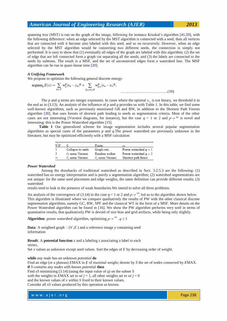
A Unifying Framework

We propose to optimize the following general discrete energy:

……………………………….(10)

The p and q terms are integer exponents. In cases where the optimal x_ is not binary, we threshold it in

the end as in (3.13). An analysis of the influence of p and q provides us with Table 1. In this table, we find some

well-known algorithms, such as previously mentioned GR and RW, in addition to the Shortest Path Forests

algorithm [20], that uses forests of shortest path leading to seeds as segmentation criteria. Most of the other

cases are not interesting (Voronoi diagrams, for instance), but the case q = 1 or 2 and p→ is novel and

interesting: this is the Power Watershed algorithm [15]. Table 1 Our generalized scheme for image segmentation includes several popular segmentation

algorithms as special cases of the parameters p and q.The power watershed are previously unknown in the

literature, but may be optimized efficiently with a MSF calculation

Power Watershed

Among the drawbacks of traditional watershed as described in Sect. 3.2.5.3 are the following: (1) watershed has no energy interpretation and is purely a segmentation algorithm; (2) watershed segmentations are

not unique: for the same seed placement and edge weights, the same definition can provide different results; (3)

watershed

results tend to leak in the presence of weak boundaries.We intend to solve all three problems.

An analysis of the convergence of (3.14) in the case q = 1 or 2 and p→ led us to the algorithm shown below.

This algorithm is illustrated where we compare qualitatively the results of PW with the other classical discrete

segmentation algorithms, namely GC, RW, SPF and the classical WT in the form of a MSF. More details on the Power Watershed algorithm can be found in [16]. We show the PW algorithm performs very well in terms of

quantitative results, that qualitatively PW is devoid of size bias and grid artifacts, while being only slightly.

Algorithm: power watershed algorithm, optimizing p→ ,q ≥ 1

Data: A weighted graph (V ,E ) and a reference image y containing seed

information

Result: A potential function x and a labeling s associating a label to each

vertex.

Set x values as unknown except seed values. Sort the edges of E by decreasing order of weight.

while any node has an unknown potential do

Find an edge (or a plateau) EMAX in E of maximal weight; denote by S the set of nodes connected by EMAX.

if S contains any nodes with known potential then

Find xS minimizing (3.14) (using the input value of q) on the subset S

with the weights in EMAX set to wi j = 1, all other weights set to wi j = 0

and the known values of x within S fixed to their known values.

Consider all xS values produced by this operation as known.



Page 239

else

Merge all of the nodes in S into a single node, such that when the value of x for this merged node becomes

known, all merged nodes are assigned the same value of x and considered known. Set si = 1 if xi ≥ 12 and si = 0

otherwise.

Fig. 5. Illustration of the different steps for Algorithm in the case q = 2. The values on the nodes correspond to x, their color to s. The bold edges represents edges belonging to a Maximum Spanning Forest. (a) A weighted

graph with two seeds, all maxima of the weight function are seeded, (b) First step, the edges of maximum

weight are added to the forest, (c) After several steps,the next largest edge set belongs to a plateau connected to

two labeled trees, (d) Minimize (3.14) on the subset (considering the merged nodes as a unique node) with q = 2

(i.e., solution of the Random Walker problem), (e) Another plateau connected to three labeled vertices is

encountered, and (f) Final solutions x and s obtained after few more steps. The q-cut, which is also an MSF cut,

is represented in dashed lines

slower than standard watershed and much faster than either GC or RW, particularly in 3D. The PW algorithm

provides a unique unambiguous result, and an energy interpretation for watershed, which allows it to be used in

wider contexts as a solver, for instance in filtering [17] and surface reconstruction. One chief advantage of PW with respect with GC for instance, is its ability to compute a globally optimal result in the presence of multiple

labels. When segmenting multiple objects this can be important.

Fig. 6. Slides of a 3D lung segmentation. The foreground seed used for this image is a small rectangle in one

slice of each lung, and the background seed is the frame of the image (a) GC (b) RW(c) SPF (d) MSF (e) PW

IV. RESULTS

Comparisons of four different filters at α= 0 and at α= 45° are shown in Figures 8 and 9, respectively.

The four filters are the square-shaped median, LOCO, and averaging filters and the plus-shaped median filter.

Significant differences among the responses of these filters are easily observed. The corner ―passband‖ and

―stopband‖ information for these filters are collected in Table below. The ―perfect rejection‖ and ―perfect

preservation‖ bands correspond to regions of where r(,α) = 0 and r(,α) = 1 respectively.



Page 240

Figure 7. Comparison of fractional corner preservation of square-shaped median, LOCO, and averaging filters

and the plus-shaped median filter at corner rotations α= 0.

Figure 8. Comparison of fractional corner preservation of square-shaped median, LOCO, and averaging filters

and the plus-shaped median filter at corner rotations α= 45°.



Page 241

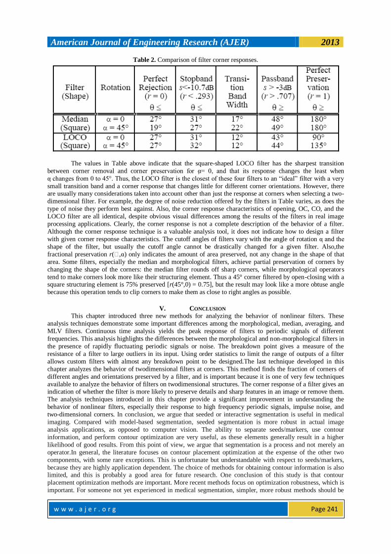
Table 2. Comparison of filter corner responses.

The values in Table above indicate that the square-shaped LOCO filter has the sharpest transition

between corner removal and corner preservation for α= 0, and that its response changes the least when

α changes from 0 to 45°. Thus, the LOCO filter is the closest of these four filters to an ―ideal‖ filter with a very

small transition band and a corner response that changes little for different corner orientations. However, there are usually many considerations taken into account other than just the response at corners when selecting a two-

dimensional filter. For example, the degree of noise reduction offered by the filters in Table varies, as does the

type of noise they perform best against. Also, the corner response characteristics of opening, OC, CO, and the

LOCO filter are all identical, despite obvious visual differences among the results of the filters in real image

processing applications. Clearly, the corner response is not a complete description of the behavior of a filter.

Although the corner response technique is a valuable analysis tool, it does not indicate how to design a filter

with given corner response characteristics. The cutoff angles of filters vary with the angle of rotation α and the

shape of the filter, but usually the cutoff angle cannot be drastically changed for a given filter. Also,the

fractional preservation r(,α) only indicates the amount of area preserved, not any change in the shape of that

area. Some filters, especially the median and morphological filters, achieve partial preservation of corners by

changing the shape of the corners: the median filter rounds off sharp corners, while morphological operators

tend to make corners look more like their structuring element. Thus a 45° corner filtered by open-closing with a square structuring element is 75% preserved [r(45°,0) = 0.75], but the result may look like a more obtuse angle

because this operation tends to clip corners to make them as close to right angles as possible.

V. CONCLUSION

This chapter introduced three new methods for analyzing the behavior of nonlinear filters. These

analysis techniques demonstrate some important differences among the morphological, median, averaging, and

MLV filters. Continuous time analysis yields the peak response of filters to periodic signals of different

frequencies. This analysis highlights the differences between the morphological and non-morphological filters in

the presence of rapidly fluctuating periodic signals or noise. The breakdown point gives a measure of the

resistance of a filter to large outliers in its input. Using order statistics to limit the range of outputs of a filter

allows custom filters with almost any breakdown point to be designed.The last technique developed in this

chapter analyzes the behavior of twodimensional filters at corners. This method finds the fraction of corners of

different angles and orientations preserved by a filter, and is important because it is one of very few techniques

available to analyze the behavior of filters on twodimensional structures. The corner response of a filter gives an indication of whether the filter is more likely to preserve details and sharp features in an image or remove them.

The analysis techniques introduced in this chapter provide a significant improvement in understanding the

behavior of nonlinear filters, especially their response to high frequency periodic signals, impulse noise, and

two-dimensional corners. In conclusion, we argue that seeded or interactive segmentation is useful in medical

imaging. Compared with model-based segmentation, seeded segmentation is more robust in actual image

analysis applications, as opposed to computer vision. The ability to separate seeds/markers, use contour

information, and perform contour optimization are very useful, as these elements generally result in a higher

likelihood of good results. From this point of view, we argue that segmentation is a process and not merely an

operator.In general, the literature focuses on contour placement optimization at the expense of the other two

components, with some rare exceptions. This is unfortunate but understandable with respect to seeds/markers,

because they are highly application dependent. The choice of methods for obtaining contour information is also limited, and this is probably a good area for future research. One conclusion of this study is that contour

placement optimization methods are important. More recent methods focus on optimization robustness, which is

important. For someone not yet experienced in medical segmentation, simpler, more robust methods should be



Page 242

preferred over complex ones. Among those, power-watershed is a good candidate because of its combination of

speed, relative robustness, ability to cope with multiple labels, absence of bias and availability (the code is

easily available online). The random walker is also a very good solution, but is not generally and freely

available. We have not surveyed or compared methods that encompass shape constraints.We recognize that this

is important in some medical segmentation methods, but this would require another study altogether.

REFERENCES

[1] Adams, R., Bischof, L.: Seeded region growing. IEEE Trans. Pattern Anal. Mach. Intell. 16(6), 641–647

(1994)

[2] Appleton, B.: Globally minimal contours and surfaces for image segmentation. Ph.D. thesis, University

of Queensland (2004). Http://espace.library.uq.edu.au/eserv/UQ:9759/ba thesis.pdf

[3] Appleton, B., Sun, C.: Circular shortest paths by branch and bound. Pattern Recognit. 36(11), 2513–2520 (2003)

[4] Appleton, B., Talbot, H.: Globally optimal geodesic active contours. J. Math. Imaging Vis. 23, 67–86

(2005)

[5] Ardon, R., Cohen, L.: Fast constrained surface extraction by minimal paths. Int. J. Comput. Vis. 69(1),

127–136 (2006)

[6] Beucher, S., Lantu´ejoul, C.: Use of watersheds in contour detection. In: International Workshop on

Image Processing. CCETT/IRISA, Rennes, France (1979)

[7] Boykov, Y., Kolmogorov, V.: An experimental comparison of min-cut/max- flow algorithms for energy

minimization in vision. PAMI 26(9), 1124–1137 (2004)

[8] Boykov, Y., Veksler, O., Zabih, R.: Fast approximate energy minimization via graph cuts. IEEE Trans.

Pattern Anal. Mach. Intell. 23(11), 1222–1239 (2001) [9] Canny, J.: A computational approach to edge detection. IEEE Trans. Pattern Anal.Mach. Intell. 8(6),

679–698 (1986)

[10] Caselles, V., Kimmel, R., Sapiro, G.: Geodesic active contours. Int. J. Comput. Vis. 22(1), 61–79 (1997)

[11] Chambolle, A.: An algorithm for total variation minimization and applications. J. Math. Imaging Vis.

20(1–2), 89–97 (2004)

[12] Chan, T., Bresson, X.: Continuous convex relaxation methods for image processing. In: Proceedings of

ICIP 2010 (2010). Keynote talk, http://www.icip2010.org/file/Keynote/ICIP

[13] Chan, T., Vese, L.: Active contours without edges. IEEE Trans. Image Process. 10(2), 266–277 (2001)

[14] Cohen, L.D., Kimmel, R.: Global minimum for active contour models: A minimal path approach. Int. J.

Comput. Vis. 24(1), 57–78 (1997). URL citeseer.nj.nec.com/cohen97global. html

[15] Couprie, C., Grady, L., Najman, L., Talbot, H.: Power watersheds: A new image segmentation

framework extending graph cuts, random walker and optimal spanning forest. In: Proceedings of ICCV 2009, pp. 731–738. IEEE, Kyoto, Japan (2009)

[16] Couprie, C., Grady, L., Najman, L., Talbot, H.: Power watersheds: A unifying graph-based optimization

framework. IEEE Transactions on Pattern Analysis and Machine Intelligence, 33(7), 1384–1399 (2011)

[17] Couprie, C., Grady, L., Talbot, H., Najman, L.: Anisotropic diffusion using power watersheds. In:

Proceedings of the International Conference on Image Processing (ICIP), pp. 4153–4156. Honk-Kong

(2010)

[18] Couprie, C., Grady, L., Talbot, H., Najman, L.: Combinatorial continuous maximum flows. SIAM J.

Imaging Sci. (2010). URL http://arxiv.org/abs/1010.2733. In revision

[19] Cousty, J., Bertrand, G., Najman, L., Couprie, M.:Watershed cuts: Minimum spanning forests and the

drop of water principle. In: IEEE Transactions on Pattern Analysis and Machine Intelligence, pp. 1362–

1374. (2008) [20] Cousty, J., Bertrand, G., Najman, L., Couprie, M.: Watershed cuts: Thinnings, shortest-path forests and

topological watersheds. IEEE Trans. Pattern Anal. Mach. Intell. 32(5), 925–939 (2010)

[21] Cserti, J.: Application of the lattice Green’s function for calculating the resistance of an infinite network

of resistors. Am. J. Phys. 68, 896 (2000)

[22] Daragon, X., Couprie, M., Bertrand, G.: Marching chains algorithm for Alexandroff- Khalimsky spaces.

In: SPIE Vision Geometry XI, vol. 4794, pp. 51–62 (2002)

[23] Dougherty, E., Lotufo, R.: Hands-on Morphological Image Processing. SPIE press, Bellingham (2003)

[24] Doyle, P., Snell, J.: Random Walks and Electric Networks. Carus Mathematical Monographs, vol. 22, p.

52. Mathematical Association of America, Washington, DC (1984)

[25] Ford, J.L.R., Fulkerson, D.R.: Flows in Networks. Princeton University Press, Princeton, NJ (1962)

[26] Geman, S., Geman, D.: Stochastic relaxation, gibbs distributions, and the bayesian restoration of images.

PAMI 6, 721–741 (1984)



Page 243

[27] Goldberg, A., Tarjan, R.: A new approach to the maximum-flow problem. J. ACM 35, 921–940 (1988)

[28] Goldenberg, R., Kimmel, R., Rivlin, E., Rudzsky, M.: Fast geodesic active contours. IEEE Trans. Image

Process. 10(10), 1467–1475 (2001)

[29] Grady, L.: Multilabel random walker image segmentation using prior models. In: Computer Vision and

Pattern Recognition, IEEE Computer Society Conference, vol. 1, pp. 763–770 (2005). DOI

http://doi.ieeecomputersociety.org/10.1109/CVPR.2005.239

[30] Grady, L.: Computing exact discrete minimal surfaces: Extending and solving the shortest path problem in 3D with application to segmentation. In: Computer Vision and Pattern Recognition, 2006 IEEE

Computer Society Conference, vol. 1, pp. 69–78. IEEE (2006)

[31] Grady, L.: Random walks for image segmentation. IEEE Trans. Pattern Anal. Mach. Intell. 28(11), 1768–

1783 (2006)

[32] Grady, L., Funka-Lea, G.: Multi-label image segmentation for medical applications based on graph-

theoretic electrical potentials. In: Computer Vision and Mathematical Methods in Medical and

Biomedical Image Analysis, pp. 230–245. (2004)

[33] Grady, L., Polimeni, J.: Discrete Calculus: Applied Analysis on Graphs for Computational Science.

Springer Publishing Company, Incorporated, New York (2010)

[34] Grady, L., Schwartz, E.: Isoperimetric graph partitioning for image segmentation. Pattern Anal. Mach.

Intell. IEEE Trans. 28(3), 469–475 (2006)

[35] Guigues, L., Cocquerez, J., Le Men, H.: Scale-sets image analysis. Int. J. Comput. Vis. 68(3), 289–317 (2006)

[36] Horowitz, S., Pavlidis, T.: Picture segmentation by a directed split-and-merge procedure. In: Proceedings

of the Second International Joint Conference on Pattern Recognition, vol. 424, p. 433 (1974)

[37] Iri, M.: Survey of Mathematical Programming. North-Holland, Amsterdam (1979)

[38] Kakutani, S.: Markov processes and the Dirichlet problem. In: Proceedings of the Japan Academy, vol.

21, pp. 227–233 (1945)

[39] Kass, M., Witkin, A., Terzopoulos, D.: Snakes: Active contour models. Int. J. Comput. Vis. 1, 321–331

(1988)

[40] Khalimsky, E., Kopperman, R., Meyer, P.: Computer graphics and connected topologies on finite ordered

sets. Topol. Appl. 36(1), 1–17 (1990)

[41] Kruskal, J.J.: On the shortest spanning subtree of a graph and the travelling salesman problem. Proc. AMS 7(1) (1956)

[42] Levinshtein, A., Stere, A., Kutulakos, K., Fleet, D., Dickinson, S., Siddiqi, K.: Turbopixels: Fast

superpixels using geometric flows. Pattern Anal. Mach. Intell. IEEE Trans. 31(12), 2290–2297 (2009)

[43] Malladi, R., Sethian, J., Vemuri, B.: Shape modelling with front propagation: A level set approach. IEEE

Trans. Pattern Anal. Mach. Intell. 17(2), 158–175 (1995)

[44] I. Pitas and A. N. Venetsanopoulos, Nonlinear Digital Filters: Principles and Applications. Boston:

Kluwer Academic, 1990.

[45] A. V. Oppenheim and R. W. Schafer, Discrete-Time Signal Processing. Englewood Cliffs, New Jersey:

Prentice Hall, 1989.

[46] J. W. Tukey, Exploratory Data Analysis. Reading, Massachusetts: Addison-Wesley, 1971.

[47] R. P. Borda and J. D. Frost, Jr., ―Error reduction in small sample averaging through the use of the median

rather than the mean,‖ Electroencephalography and Clinical Neurophysiology, vol. 25, pp. 391- 392, 1968.

[48] P. Maragos and R. W. Schafer, ―Morphological filters—Part I: Their settheoretic analysis and relations to

linear shift-invariant filters,‖ IEEE Trans. Acoust., Speech, Signal Process., vol. 35, no. 8, pp. 1153-1169,

[49] 1987.P. Maragos and R. W. Schafer, ―Morphological filters—Part II: Their relations to median, order-

statistic, and stack filters,‖ IEEE Trans. Acoust., Speech, Signal Process., vol. 35, no. 8, pp. 1170-1184,

1987.

[50] B. I. Justusson, ―Median filtering: Statistical properties,‖ in Two- Dimensional Digital Signal Processing

II: Transforms and Median Filtering, T. S. Huang, Editor. Berlin: Springer-Verlag, 1981. pp. 161- 196.

[51] S. G. Tyan, ―Median filtering: Deterministic properties,‖ in Two- Dimensional Digital Signal Processing

II: Transforms and Median Filtering, T. S. Huang, Editor. Berlin: Springer-Verlag, 1981. pp. 197- 217.

[52] N. C. Gallagher, Jr. and G. L. Wise, ―A theoretical analysis of the properties of the median filter,‖ IEEE Trans. Acoust., Speech, Signal Process., vol. 29, no. 6, pp. 1136-1141, 1981.

[53] G. Matheron, Random Sets and Integral Geometry. New York: Wiley, 1974. 53. J. Serra, Image Analysis

and Mathematical Morphology, Vol. 1. London: Academic, 1982.

[54] J. Serra, Editor. Image Analysis and Mathematical Morphology, Vol. 2: Theoretical Advances. London:

Academic, 1988.



Page 244

[55] R. L. Stevenson and G. R. Arce, ―Morphological filters: Statistics and further syntactic properties,‖ IEEE

Trans. Circuits Syst., vol. 34, no. 11, pp. 1292-1305, 1987.

[56] G. Gerig, O. Kübler, R. Kikinis, and F. A. Jolesz, ―Nonlinear anisotropic filtering of MRI data,‖ IEEE

Trans. Med. Imag., vol. 11, no. 2, pp. 221- 232, 1992.

[57] 57. S. R. Sternberg, ―Biomedical image processing,‖ IEEE Computer, vol. 16, no. 1, pp. 22-34, 1983.

[58] S. R. Sternberg, ―Grayscale morphology,‖ Comp. Vision, Graphics, Image Process., vol. 35, pp. 333-355,

1986. [59] P. D. Wendt, E. J. Coyle, and N. C. Gallagher, ―Stack filters,‖ IEEE Trans. Acoust., Speech, Signal

Process., vol. 34, no. 4, pp. 898-911, 1986.

[60] J. P. Fitch, E. J. Coyle, and N. C. Gallagher, ―Median filtering by threshold decomposition,‖ IEEE Trans.

Acoust., Speech, Signal Process., vol. 32, pp. 1183-1188, 1984.

[61] J. P. Fitch, E. J. Coyle, and N. C. Gallagher, ―Threshold decomposition of multidimensional ranked order

operations,‖ IEEE Trans. Circuits Syst., vol. 32, pp. 445-450, 1985.

[62] E. J. Coyle and J.-H. Lin, ―Stack filters and the mean absolute error criterion,‖ IEEE Trans. Acoust.,

Speech, Signal Process., vol. 36, no. 8, pp. 1244-1254, 1988.

[63] H. A. David, Order Statistics, 1st ed. New York: Wiley, 1970.

[64] R. V. Hogg and A. T. Craig, Introduction to Mathematical Statistics. 4th ed. New York: Macmillan, 1978.

[65] L. Koskinen, J. Astola, and Y. Neuvo, ―Morphological filtering of noisy images,‖ in Visual

Communications and Image Processing „90, M. Kunt, Editor, Proc. SPIE, vol. 1360, pp. 155-165, 1990. [66] J. Astola, L. Koskinen, and Y. Neuvo, ―Statistical properties of discrete morphological filters,‖ in

Mathematical Morphology in Image Processing, E. R. Dougherty, Editor. New York: Marcel Dekker,

1993. pp. 93-120.

biomedical image processing with morphology and …7)/za27227244.pdf · american journal of...

Documents