biomass accumulation model - globe.gov

GLOBE® 2017 Biomass Accumulation Model - 1 Biosphere

Appendix

Welcom

eIntroduction

ProtocolsLearning A

ctivitiesBiomass Accumulation Model Predicting Net Primary Productivity and Biomass using Temperature, Precipitaion and Biomes

!?

Purpose• To experience using a computer model• To understand how a simple model

can describe emergent properties of a complex system

• To draw conclusions about how variations in model parameters affect the resulting predictions.

• To recognize the utility and limitations of a simple model

OverviewIn this activity, students will learn to use a simple model which uses annual temperature and precipitation, to predict net primary productivity (net plant growth), and then adds in turnover rate approximated from biome type to calculate biomass, and carbon storage. This model has been used in both science and education, and can help introduce students to not only modeling concepts, but can allow them to hypothesize about the behavior of ecosystems.

Student OutcomesStudents will be able to:• Use a simple computer model to conduct

research investigations• Identify the effects of each model variable

through isolation testing• Describe activity results by correctly using

modeling concepts• Discuss limitations and assumptions of

this model• Relate their work on this model to other

topics

QuestionsEssential• How are models useful in understanding

the Science?Unit• See Unit Assessment section for unit

question ideas. Content• How are temperature and precipitation

used to predict NPP?• How was turnover rate determined for

this model?• Where does this model fit within the global

carbon cycle?• What are the model’s limitations and as-

sumptions?

Science ConceptsGrades 5-8Scientific Inquiry• Design and conduct a scientific investiga-

tion.• Use appropriate tools and techniques to

gather, analyze, and interpret data.• Develop descriptions, explanations, pre-

dictions, and models using evidence.• Think critically and logically to make the

relationships between evidence and ex-planations.

• Communicate scientific procedures and explanations.

History and Nature of Science• Scientists formulate and test their ex-

planations of nature using observation, experiments, and theoretical and math-ematical models.

Grades 9-12Scientific Inquiry• Design and conduct a scientific investiga-

tion.• Use technology and mathematics to im-

prove investigations and communicationsScience and Technology• Science often advances with the intro-

duction of new technologies. Solving technological problems often results in new scientific knowledge.

Science in Personal and Social Perspectives• Science and technology can only indicate

what can happen, not what should hap-pen.

History and Nature of Science• Individuals and teams have contributed

and will continue to contribute to the sci-entific enterprise.

• Because all scientific ideas depend on experimental and observation confirma-tion, all scientific knowledge is, in prin-ciple, subject to change as new evidence becomes available.


BackgroundScientists use computer models to help them understand the behavior of complex systems and to predict outcomes that cannot be measured directly. Models can be written at many levels of detail, from the very simple to the very complex. Not surprisingly, there is often a tradeoff between the ease with which a model can be understood and used and the number of properties that can be reliably predicted. The biomass accumulation model is very simple in that it only responds to variation in these two climate variables and all forms of aboveg-round biomass (leaves, stems, branches and bark) are lumped into a single box, known as the biomass pool, or standing stock.The model is based on the work of H. Leith and R. Whittaker (1975) who realized that, de-spite the high degree of local variability that can be exhibited by ecosystems, at broader spa-

Earth Science• The earth is a system…each element on

earth moves among reservoirs in the solid earth, oceans, atmosphere, and organ-isms as part of geochemical cycles

NGSS (Black- covered directly, gray-ad-dressed, but not directly covered)

• Disciplinary Core Ideas ◦ Gr.6-8: LS2.C, ESS3.A, ETS1.B, ETS.C, LS2.A, LS2.B, ESS3.C

◦ Gr.9-12: LS2.B, LS2.C, LS2.A ESS3.A, ESS3.C, ETS1.B, ETS.C

• Science and Engineering Practices ◦ Asking Questions ◦ Developing and using models ◦ Planning and carrying out investigations ◦ Analyzing and interpreting data ◦ Using mathematics and computational thinking

◦ Constructing explanations ◦ Obtaining, Evaluating, and Communi-cating Information

• Crosscutting Concepts: ◦ Patterns ◦ Cause and Effect ◦ Scale, Proportion, and Quantity ◦ Systems and System Models ◦ Stability and Change

Time/Frequency 160 minutes, additional time for extensions

LevelSecondary (Middle & High School)

Materials and Tools• Computers (one per student pair)• Access to online Biomass Accumulation

Model hosted by the isee Exchange (https://exchange.iseesystems.com/public/globeprogam/biomass-accumulation-model)

• Biomass Accumulation Model Student Worksheets 1 and 2 (one per student)

• Graph paper (2 sheets per student)• Sketch of Biomass Accumulation Model

box - arrow diagram on the board.• Biome Figures (class copies-LCD,

overhead, or laminated handouts)

Prerequisites• Ability to use an online computer model.

Review the Paperclip Tutorial Model if necessary. (https://exchange.iseesystems.com/public/globeprogam/paperclip-tutorial-model)

• Basic knowledge of modeling or systems dynamics (see Paperclip Tutorial Model).

• Biomass Units activity (optional). • Ability to make a variety of unit conver-

sions: Fahrenheit to Celsius, inches to millimeters, pounds to kilograms, fractions and their reciprocals.

• Basic knowledge of the carbon cycle (see Global Carbon Cycle Introduction).

Preparation• Review modeling terms: stock, pool, res-

ervoir, flux, proportional rate, equilibrium, steady state, turnover rate.

• Optional: review the Carbon Cycle Modeling eTraining (https://www.globe.gov/get-trained/protocol-etraining/etraining-modules/16867717/3099387)

• Make appropriate copies• Set up computers• Write essential, unit, and content ques-

tions somewhere visible in the classroom.• Write essential, unit, and content ques-

tions somewhere visible in the classroom.

https://exchange.iseesystems.com/public/globeprogam/biomass-accumulation-model

https://exchange.iseesystems.com/public/globeprogam/biomass-accumulation-model

https://exchange.iseesystems.com/public/globeprogam/paperclip-tutorial-model



https://www.globe.gov/get-trained/protocol-etraining/etraining-modules/16867717/3099387




Appendix

Welcom

eIntroduction

ProtocolsLearning A

ctivitiestial scales, biome distribution and rates of productivity fol-low predictable patterns with mean annual temperature and mean annual rainfall. Simple mathematical equa-tions describing these pat-terns form the basis of the model used here. Although there are other important factors the model does not include (e.g. nutrients, soil type, insect pests, seasonal climate variation), it provides a firm foundation for examin-ing one important part of the global carbon cycle.

Biomass is the total mass of living material, usually expressed in units of mass per unit land area (grams per meter squared [g/m2] or kilograms per hectare [kg/ha]). Because a large fraction of living biomass consists of water and because the percentage of water can vary widely through time and from species to species, biomass is expressed as a dry weight. Dry weight is determined after all water has been removed from sample plant material in a drying oven. Total biomass is found by summing the dry weight biomass of all individuals in a given land area. About 50% of all biomass by dry weight is carbon. It is important to understand the distinctions between biomass, biomass production (or growth), and biomass accumula-tion. The concept of biomass itself is straightforward and is usually easily grasped because it is simply the standing stock of material. Biomass production, or growth, is the rate at which biomass is produced per unit time. The production of new biomass is typically referred to as net primary production (NPP), which can be thought of as the total rate of growth of all plant tissues over a specific time period (NPP is reported usually in units of g/m2 yr or kg/ha yr). Biomass accumulation is the net change in standing biomass from one time to another (g/m2). This is often confused with growth or NPP because the accumulation of biomass is a direct result of growth. But how biomass actually changes from one time to another is the net difference between how much is added from growth and how much is lost from death (death of whole plants as well as twigs, branches, etc.).

In a young forest, for example, biomass can accumulate rapidly because the rate of growth is typically much greater than the rate of litter production (plant death) (Figure 1). But as for-ests age, the growth rate changes relatively little, while the rate of litter production increases (because the turnover rate—the fraction of biomass that dies each year—applies to a larger and larger biomass pool as time goes on). As this happens, the accumulation of biomass slows and eventually reaches zero. Zero net accumulation occurs when the average annual death rate equals the average annual growth rate, preventing any further accumulation. At this point, the forest has reached a condition of steady state, or equilibrium. Based on this description, we see that the maximum amount of biomass that can occur in any ecosystem at steady-state is a function of both the growth rate (NPP) and the death rate (the turnover rate).

Finally, because we assume that the carbon content of all biomass remains constant at 50% (which is a close approximation of reality), any of the above terms (biomass, NPP, or biomass accumulation) can be expressed as a mass of dry biomass or as a mass of carbon. This means that NPP kg (biomass)/ha yr times 0.50 equals NPP in kgC/ha yr. Biomass in g/m2 yr times 0.50 equals what we refer to as carbon storage, gC/m2 yr.

Figure 1. Biomass Accumulation slows as the ecosystem reaches equilibrium


Climate Variables: NPP in the world’s ecosystems can be in-fluenced by a wide variety of factors including climate (tem-perature and precipitation), so-lar radiation, soil type, nutrient availability, and disturbance from fire, herbivores (e.g. insects and grazing animals), and human management. Because a model that included the effects of all of these factors would be compli-cated and difficult to obtain input data for, the model used in this exercise focuses on the effects of the two most important climate variables; temperature and pre-cipitation. Some degree of vari-ation between predicted growth rates and those observed at a given field site is expected given the influence of other factors the model doesn’t include. The global-scale pattern of how NPP and biome distribution varies with mean annual temper-ature (MAT) and mean annual precipitation (MAP) was first defined in 1975 by the research of H. Leith and R. Whittaker and form the basis of the model (Figure 3). To run the model you will need to enter your biome type along with values for average annual temperature and precipitation for a given location. Note from the curves in Figure 3 that temperature and pre-cipitation will each produce a unique estimate of NPP. In the mode, these are referred to as NPP-T for the temperature-based estimate and NPP-P for the precipitation-based estimate. For each location, the model compares these NPP values and chooses the smaller of the two as its estimated rate of NPP. If NPP-T is smaller than NPP-P, we can assume that growth rates are limited by temperature and that no additional amount of rainfall will cause a growth increase. Conversely, a lower value of NPP-P implies a water limitation. As in many of the world’s regions, higher temperatures do not produce higher growth rates when water is the limiting resource.Find your local Climate Variables: There are many ways to obtain estimates of MAT and MAP for your sites. A few suggestions are listed below.

Figure 2. The global distribution of major ecosystems with respect to mean annual temperature and mean annual precipitation. From Ollinger 2002, modified from Whittaker, 1975.

Figure 3. The relationship between net primary production and (a) annual temperature and (b) annual precipitation for ecosystems around the world. From Leith 1975.


Appendix

Welcom

eIntroduction

ProtocolsLearning A

ctivities

1. Climate and Biome Resource Page. https://www.globe.gov/documents/355050/41927208/Biomass+Accumulation+Model+Resources. This resource page contains multiple tools and directions for finding your local biome, annual temperature and precipitation. The page is also available from the Biomass Accumulation Model by clicking on the ‘Climate Data’ button from the Model Variables page.

2. Local weather station. In this case you will want a 30-year average of annual tempera-ture in degrees C and total annual rainfall in millimeters. These data and other climate variables can be accessed through the web sites of several climate data networks. A few examples are: the U.S. National Climate Data Center (http://www.ncdc.noaa.gov/), the World Meteorological Organization (http://www.wmo.int) and the United Nations Food and Agricultural Organization (http://www.fao.org).

3. Your data. If your site has had a weather station operating for 10 years or more (over all seasons) you can calculate the long-term average temperature and precipitation for your site.

Turnover Rate: The turnover rate is the rate at which living plant material dies and becomes plant litter (dead leaves, wood, roots, etc. which later become incorporated into soils). This is usually determined as the ratio of the amount of dead plant litter produced in a given year to the total amount of plant biomass present (the “standing stock” or “pool size” of plant bio-mass). In some cases, plants only live for one year or less (plants known as “annuals”). For these plants, their entire biomass dies each year, so the turnover rate is 1. In other words, 100% of their total biomass “turns over” each year. For plants that live more than a year (called “perennials”), the turnover rate will usually be some number between 0 and 1. For example, for many grasses, the aboveground portion of the plant dies each year, but the roots can persist from one year to the next. Hence, the turnover rate for grasslands might be closer to 0.5, meaning that 50% of total biomass dies each year. For much larger and longer-lived plants like trees (some of which can live for hundreds or even thousands of years!), plant litter produced each year (twigs and branches that die and fall to the ground) is often a small fraction of the total biomass. The turnover rate in forests can be as low as 0.02 (2 % of standing live biomass dies each year). Because turnover rate is so closely tied to vegetation type, in this model we use biome classifications to consider typical turnover rates around the world. Turnover rates in this model come largely from global ecosystem studies by Amthor et al (1998), and additional rates come from Aber and Mellilo (2001).

As a final note, an approximation of turnover rate can be estimated even in situations where death rate has not been independently calculated. This is possible if the amount of dead plant litter produced each year is equal to the amount of new plant biomass that is grown. This occurs when an ecosystem has matured and is no longer accumulating biomass, such as in an old-growth forest. In these cases, the turnover rate can be estimated using the growth rate divided into the total biomass because this will yield the same number as the death rate divided into the total biomass. (See the Systems & Modeling Introduction on the GLOBE Carbon Cycle webpage Resources section for more information.)

Find your local Turnover Rate: In order to complete this exercise, you’ll need to know the turnover rate for your site of interest. Listed below are several ways you can find this infor-mation.

1. Model Table. Within the model (From the Model Variables page, click on ‘Turnover Rate’) the legend provided under the biome map gives average turnover rates for the major world biomes (note that these are only averages and may differ somewhat from the true value at your site). Read further if you do not know your biome:a. Gridded Database. Use the latitude and longitude lookup function discussed in

the MAT/MAP section above to determine the biome type. Click on ‘Table of 30 year Averages’ to see your biome. This is also available from the Biomass Accumulation

https://www.globe.gov/documents/355050/41927208/Biomass+Accumulation+Model+Resources

https://www.globe.gov/documents/355050/41927208/Biomass+Accumulation+Model+Resources


Model by clicking on the ‘Climate Data’ button from the Model Variables page.b. Map and Descriptions: See the biome map with expanded descriptions here:

https://www.globe.gov/documents/355050/41927208/Global+Biome+Descriptions/589a4250-9980-4b29-899c-68f9ba561dfb

a. Zoomable map. Use this online map to find your biome: https://ecoregions2017.ap-pspot.com. Click ‘Biome’ at the top of the screen and use the slider bar to adjust the map transparency.

ENGAGE Grouping: Class Time: 10 Minutes

• Use a formative assessment technique (i.e. Frayer Model, KWL) to establish student prior knowledge about systems, modeling, and/or biomass.

• If necessary, demonstrate for students how to open the Biomass Accumulation Model and get started in their investigations.

• View Biomass Accumulation Model Screencast Tutorial available from the GLOBE Car-bon Cycle website Learning Activities Modeling section, or from the Carbon Cycle Modeling eTraining (https://www.globe.gov/get-trained/protocol-etraining/etraining-mod-ules/16867717/3099387)

What To Do and How To Do It

EXPLORE Grouping: Pairs Time: 45 Minutes

• Students follow the instructions in Student Worksheet 1. Students should read the model “story”, record important concepts, respond to comprehension questions, and add to the model diagram of this system based on their reading and prior knowledge of the global carbon cycle.

EXPLAIN Grouping: Class Time: 15 Minutes

• Record and review new terms and concepts on an overhead or whiteboard. • Ask several students to share their expanded model diagrams, be sure that all students

understand what variables are contributing to the model results and how this model study relates to the bigger picture.

• Discuss: What are the limitations of this model? What variables are not included?

ELABORATE Grouping: Pairs Time: 40 Minutes

• Students follow the instructions in Student Worksheet 2: Using the Biomass Accumulation Model to Understand Your Biome to conduct a model investigation that looks at their own biome under altered turnover rate, temperature, and precipitation.

◦ Begin with a class demonstration using an LCD projector. Demonstrate an example model run following the directions in Student Worksheet 2. Show students where to find model variable input values, how to view the different graph pages and read graph results, and how to use the data table of model results.

Ø You may also want to review how to create scatter plot graphs. Ø To provide additional guidance for students complete “Activity 1” of Student Work-

sheet 2 as a class. ◦ Students work in partners to complete Student Worksheet 2. ◦ To share the workload students can pair with another group to perform “Activity 3”.



https://ecoregions2017.appspot.com

https://ecoregions2017.appspot.com




Appendix

Welcom

eIntroduction

ProtocolsLearning A

ctivities

EVALUATE Grouping: Class Time: 15 Minutes

• As a class, discuss students’ responses to Student Worksheet 2. • Help students make connections between the exercise they completed and other related

topics (global carbon cycle, field work, and climate change).• Let students know what else they could do with the model (See Extensions).

Assessment• Students should be graded on the thought-

fulness and thoroughness of their writ-ten responses and their ideas/questions shared during class discussions.

• Extension assessment: ideas are listed under each separate extension.

Unit Assessments• After completion of some or all of the

global Biomass Accumulation Model Ac-tivities and Extensions, students will have a range of knowledge (models, NPP, bio-mass, carbon storage, turnover rate, etc.). Below is a variety of questions that could be part of a unit assessment. Based on the exercises students complete and your teaching goals, select the questions that are most appropriate. (See the Appendix for Teacher Answers: Unit Assessment Questions.)

1. What is the pattern in which biomass and carbon storage increases over time?

2. What determines the upper limit of bio-mass and carbon storage in a given ecosystem?

3. If ecosystems continue to grow, why doesn’t the biomass pool increase in-definitely?

4. What do the terms biomass and Net Pri-mary Productivity mean with regard to the carbon cycle?

5. Ecosystems are often seen as a partial solution to climate change because of their capacity to take up CO2. Based on your work, do you think this is real-istic? Can this represent a long-term solution?

6. What does the model tell us about future rates of growth under climate change? Do you think ecosystems will store more

or less carbon? Will this accentuate or offset climate change?

7. After review of the global carbon cycle diagram, which global pool is the bio-mass pool most similar to? Describe what you learned about this pool.

8. What other pools might one add to the Biomass Accumulation Model to create a more complete model of carbon cy-cling? (Use this to go on to Global Car-bon Cycle models.)

Adaptations• For shorter class periods:

◦ Pre-assignment – Have students look up latitude, longitude, temperature, precipitation and biome before class.

◦ Homework – Have students complete thought questions at home. Students can discuss their answers using on-line technology such as Google docs, Moodle, discussion forums, wikis, etc.

• To differentiate learning: ◦ Modify the worksheet directions. Break the directions into smaller blocks, add screen shots from the model to make the directions more clear, or add helpful hint boxes to the page that remind stu-dents how to read the model graphs, make their own graphs, etc.

◦ Provide a pre-reading that helps put additional context around the model. Ollinger, S.V. 2002. Forest Ecosys-tems. In: Encyclopedia of Life Scienc-es. Nature Publishing Group, London.

Extensions - Increasing InquiryThe options below extend the modeling ex-perience. Each option also increases the level of inquiry from a very teacher-directed activity to a more student-directed activity. Students will have extensive opportunities to practice and improve their scientific re-

One group can perform temperature runs and the other can run precipitation changes. Each group should share their data so they can discuss the questions together.


search skills throughout the progression. • Extension 1: Compare fieldwork carbon

storage values to model values. ◦ *Pre-requisite: Collection and analy-sis of schoolyard data on biomass and carbon storage through the GLOBE Carbon Cycle Protocols.

◦ Pose this research question to stu-dents: How does the modeled carbon storage for your biome compare to the carbon storage you calculated during your fieldwork?

◦ Revisit carbon field data. If you up-loaded your data to the GLOBE web-site, you can find it using the GLOBE Visualization System (https://vis.globe.gov).

◦ As a class, design and investigation plan to answer the research question (based on making model runs and the available field data).

◦ Students work in pairs to conduct the investigation, including recording data and performing a basic analysis of their results. Were they able to answer the research question? How do model results compare to field data? Suggest reasons for any differences between model results and field data.

◦ Further discuss model results as a class.

• Extension 2: NPP, biomass, and carbon storage predictions for biomes around the world.

◦ *Pre-requisite: Some study of world bi-omes.

◦ Students pose their own research question, on the topic of comparing dif-ferent biome’s NPP, biomass, and car-bon storage.

◦ Students work in partners to develop an investigation plan and design a data table to record data.

◦ Students then conduct their investiga-tion and analyze model results in rela-tion to their research question. Analy-sis should include data tables, graphs, and a brief summary of their findings.

◦ Student pairs share their findings with the class through a 5-7min presenta-tion of their research.

◦ Each pair should also identify one new research question that came about

from their results. ◦ To see an animation of the Biomass Accumulation Model run for the en-tire globe under both current and fu-ture climate conditions, please visit: http://studentclimatedata.unh.edu/anima-tions.shtml and follow the links under the ‘Biomass Accumulation Animation’ heading.

• Extension 3: Predicted NPP under chang-ing climate conditions.

◦ *Pre-requisite: knowledge on climate change (temperature, precipitation, and the carbon cycle).

◦ Students complete Student Worksheet 3 -Extension: Using the Biomass Ac-cumulation Model to Explore Climate Change to explore how changes in temperature and precipitation, predict-ed to occur with climate change might influence NPP, biomass and carbon storage in one or multiple biomes.

◦ Students pose a research question, develop an investigation plan (by using the “Advanced Inputs” - climate change variable dials in the model) then inves-tigate and analyze results.

Ø Climate change data: The Stu-dent Climate Data website (http://studentclimatedata.unh.edu) provides resources for students to develop their own research projects in Student Worksheet 3. From the home page, navigate to the ‘Data Resources’ tab to find current and future climate maps, animations of changes in climate over time, climate data for a spe-cific location, etc.

◦ Students may want to connect their findings with the most recent climate change reports (local, regional, nation-al, international – IPCC) and/or write a more formal report of their findings (with data and graphs), which includes possible ecological implications to that biome if those changes occurred and identifies new research questions.

• Extension 4: Small group research. ◦ Students work in groups of 3-4 to pose a research question answerable, in part, by using results from the Biomass Model. (And perhaps other developed

https://vis.globe.gov

https://vis.globe.gov

http://studentclimatedata.unh.edu


Appendix

Welcom

eIntroduction

ProtocolsLearning A

ctivitiesmodels such as the Global Carbon Cy-cle Models). The project should also include additional research (field work, journal articles, technical reports).

◦ Students write a research report to be turned in for peer review by each of the members of one other group.

◦ Students share their final results with the class through an oral presentation that includes the use of multi-media tools.

References• Aber, J. D. and Mellilo, J. A. 2001. Terres-

trial Ecosystems.• Amthor, J.S. and members of the Eco-

systems Working Group. 1998. Terrestrial Ecosystem Responses to Global Change: a research strategy. ORNL Technical Memorandum 1998/27. Oak Ridge Na-tional Laboratory, Oak Ridge, Tennessee. 37 pp.

• Leith, H. and Whittaker, R.B. 1975. In: Pri-mary Productivity of the Biosphere, eds Leith, H. and Whittaker, R.B. (Springer, New York), pp 237–263.

• Ollinger, S.V. 2002. Forest Ecosystems. In: Encyclopedia of Life Sciences. Nature Publishing Group, London.

• Whittaker, R,H. 1975. Communities and Ecosystems. Macmillan Publishers, New York.

• World Wildlife Fund. http://www.worldwild-life.org/science/ecoregions/item1267.html

• http://www.worldwildlife.org/science/ecore-gions/delineation.html

Resources• GLOBE Carbon Cycle Modeling

eTraining: https://www.globe.gov/get-trained/protocol-etraining/etraining-mod-ules/16867717/3099387

• isee systems exchange: http://exchange.is-eesystems.com

• Cao, M. and Woodward, F.I. 1998. Net primary and ecosystem production and carbon stocks of terrestrial ecosystems and their responses to climate change. Global Change Biology, 4, 185-198.

• Climate Wizard – The Nature Conservan-cy: http://www.climatewizard.org/

• Intergovernmental Panel on Climate Change: http://www.ipcc.ch/

• Student Climate Data: http://studentclimatedata.unh.edu




http://exchange.iseesystems.com

http://exchange.iseesystems.com


TEACHER VERSION

(Suggested student responses included)

Unit Assessment Questions

1. What is the pattern in which biomass and carbon storage increases over time? Biomass accumulates quickly at first (steep line), and then accumulation slows, eventually reaching a maximum where model inputs equal model outputs (flat line). This happens because, while the inputs are constant, the outputs grow as the size of the biomass pool grows. Carbon follows the same pattern because it is simply calculated as 50% of the biomass value in any given year. This pattern is driven by growth rate, litterfall and turnover rate.

2. What determines the upper limit of biomass and carbon storage in a given ecosys-tem?

The upper limit of biomass and carbon storage is ultimately dependent on the growth rate (NPP) and turnover rate of the ecosystem. A change in either of these values will result in a change in the upper limit of biomass.

In this model, either temperature or precipitation will limit the amount of growth that can occur. In general however, there is always a limiting factor to growth. It could be a lack of available mineral nutrients in the soil, water, sunlight (strength, day length, number of growing degree days), carbon dioxide (CO2) in the sur-rounding atmosphere, or the presence of damaging factors such as insects or excessive concentrations of ozone (O3).

Although not dealt with in this activity, changes in turnover can also occur. These may be a result from changes in the lifespan or mortality rate of the biomass (i.e. plants).

3. If ecosystems continue to grow, why doesn’t the biomass pool increase indefinitely? If the growth rate (NPP) is constant and the amount of litterfall each year is calcu-lated as a fraction of the total biomass in the pool (turnover rate multiplied by pool size), as the biomass pool increases so will the amount of litter being lost. Even-tually, litterfall outputs will grow to the point where they equal NPP inputs. This is the point at which equilibrium has been reached.

4. What do the terms biomass and Net Primary Productivity mean with regard to the carbon cycle?

Biomass is the total mass of living things measured as dry weight. Carbon stor-age in an ecosystem is calculated as approximately 50% of the biomass. Bio-mass is the pool where carbon is stored.

NPP (growth) is the production of new plant biomass achieved in a given period of time. As with biomass, carbon uptake via plant growth is determined as being 50% of NPP. NPP is the flux of carbon from the atmosphere into the plant bio-mass pool.

5. Ecosystems are often seen as a partial solution to climate change because of their capacity to take up CO2. Based on your work, do you think this is realistic? Can this represent a long-term solution?

Terrestrial ecosystems do indeed take up a lot of CO2 through the process of photosynthesis. However, approximately half of the photosynthesis that occurs is offset by losses of CO2 back to the atmosphere due to plant respiration. On top of that, while plants continue to store carbon (as a sink) while they are alive and


growing, eventually all plants die and decompose or burn. During the decomposi-tion and combustion processes any carbon stored in the plants will be released back to the atmosphere, resulting in a zero net storage of carbon over the com-plete life cycle of an individual plant.

The only ways in which terrestrial ecosystems can represent a long-term carbon storage solution, as opposed to a temporary one, are under circumstances where plants are being used to permanently reclaim areas that were either previously vegetated, such as abandoned city lots, building rooftops, denuded agricultural ar-eas, etc or if the upper limit of biomass in a particular ecosystem can be increased (e.g. planting trees in grasslands). The process of re-vegetation acts by increas-ing the total amount of land area that contains carbon stored in ecosystems, this basically counteracts the original loss of carbon during deforestation and land-use change practices (currently 1.1Pg of carbon loss to the atmosphere per year). Some studies are also exploring whether the maximum biomass of existing eco-systems can increase from fertilization by atmospheric CO2 (from fossil fuel burn-ing) or soil nitrogen (N) (from wet and dry N-deposition).

6. What does the model tell us about future rates of growth under climate change? Do you think ecosystems will store more or less carbon? Will this accentuate or offset climate change?

The answer to this question depends on the climate scenarios that students choose. You may want to suggest the use of realistic scenarios such as those found in the IPCC reports. As an example if students looked at a Banff National Park in Canada, a temperate coniferous forest, they would find that if temperature increased only 2.6dg C and there were no change in precipitation the ecosystem would become precipitation limited. This would result in no drastic increase in the amount of carbon that could be stored at that site. However, if precipitation were also to increase (by 200mm) over the same 200-year time period the carbon stor-age is expected to increase by approximately 1700gC/m2, and the ecosystem has not yet reached equilibrium. This type of response would constitute a negative feedback, in that, increased warming and precipitation due to rising CO2 would in-crease biomass accumulation and carbon storage, ultimately removing additional CO2 from the atmosphere and reducing additional warming.

7. After review of the global carbon cycle diagram, which global pool is the biomass pool most similar to? Describe what you learned about this pool.

The biomass pool in the Biomass Accumulation Model is the plant pool on the global carbon cycle diagram, except that in the 1-box model we are only looking that the plant biomass for one location, whereas in the global model we are look-ing at the plant biomass of all terrestrial ecosystems on the globe.

The biomass pool is determined by the input, NPP, which is the total production of new biomass (equivalent to photosynthesis minus losses from plant respiration) and the output, litterfall (based on the biome’s turnover rate and current pool size). The amount of biomass in a plant or ecosystem is used to calculate the amount of carbon being stored there.

8. What other pools might one add to the Biomass Accumulation Model to create a more complete model of carbon cycling? (Use this to go on to Global Carbon Cycle models.)

In the one-box biomass model, you’ll note that the inputs are not drawn from an-other pool and the outputs are not added to another pool. These simply appear and disappear, making this what we could call an open model. In reality, carbon taken up by plants is drawn from the atmosphere. Hence, adding an atmosphere pool might be a logical place to start. In doing so, we would see that any increase in the plant C pool would cause a corresponding decrease in the atmosphere C


pool.

Similarly, carbon losses from living plants are normally added to soils (with the exception of fire, harvesting by humans, etc.). Addition of a soil pool would be a good choice for the growing model. Carrying this a bit further, we might also real-ize that losses from the soil result largely from decomposition, which puts C back in the atmosphere. Making that connection (atmosphere plant soil atmo-sphere) would complete the loop and give us a closed model.

Once underway, this process could result in the addition of many pools, including oceans, rivers, rocks and sediments. With these ideas in mind, students may start filling in the blanks through brainstorming to come up with the remaining pools and fluxes and a more realistic picture of the carbon cycle. (Use the Global Car-bon Cycle Diagram and Global Carbon Cycle Introductory Learning Activities as a guide.)


TEACHER VERSION


Student Worksheet 1:Learning the science behind the Biomass Accumulation Model

Task

In this exercise, you will learn about the science used to build the GLOBE Carbon Cycle Biomass Accumulation model. You should follow the instructions below to record new vocabulary and answer quick questions based on your prior knowledge and understandings gained during the model “story”.

Instructions 1. Open the Biomass Accumulation Model.

2. To learn about the science of the model, click and read the story. While you read: a. Summarize the definitions of new vocabulary in your own words. Be sure to record

all units.b. Answer quick questions to the best of your ability, you will be assessed on your

thought process.

Activity

Vocabulary 1: Carbon StorageCarbon storage is the total amount of carbon in plant tissues at a given time, which include various organic compounds: e.g. sugars including cellulose, starch, proteins, wood components such as lignin, and many others (units: grams of C per square meter).

Vocabulary 2: Carbon UptakeCarbon uptake is the amount of carbon taken out of the atmosphere in the form of carbon dioxide and used in photosynthesis resulting in plant growth over a given unit of time (units: grams of C per square meter per year).

Vocabulary 3: BiomassBiomass is the total mass of living things measured as dry weight. Typical units of biomass are grams per meter squared of land area.

How is biomass related to carbon storage?Carbon storage is calculated as approximately 50% of biomass in all living things.

Vocabulary 4: Net Primary Productivity (NPP) (also referred to as productivity)NPP (growth) is the increase of biomass minus losses that occur primarily due to respiration in a given year. NPP is measured in units of grams per meter squared per


year.How is NPP related to carbon uptake?

To calculate how much carbon plants take up during growth scientists multiply NPP by 50%.

Quick Question 1: What factors influence ecosystem vegetation growth? Locally? Globally?Your answer:

Example: Light, water, carbon dioxide, and mineral nutrients determine each plant’s growth (I know this from the Plant-a-Plant experiments). At the larger scale, such as forests worldwide I think temperature plays an important role.

How does your answer compare to the provided answer?Example: Vegetation growth is influenced by all of the things that I said but I did not consider all of the larger scale patterns of the environment: climate- temperature & precipitation, solar radiation, soil type, nutrient availability, and disturbance from many factors including fire, herbivores (insects and animals) and human land management.

In this model only the climate variables, temperature and precipitation are used to determine ecosystem growth. While this is overly simplistic and would not work for a small area such as one field site or the school yard these two variables are the most reliable when trying to predict NPP at the global scale. There is a well-defined global relationship between temperature and productivity as well as precipitation and productivity, this means that even when data is not available for a specific location we can use the data created equations (as seen in this model) to provide us with a best estimate of NPP. At small scales, specific soil type or exact sunlight availability may play a much larger role in growth differences because the whole area has received the same amount of precipitation and has the same mean annual temperature.

Quick Question 2: Brainstorm where/how you might be able to obtain mean annual temperature and precipitation data. Suggest at least two possible ideas.

Climate data can be obtained from a global database, where scientists have compiled data from many studies, such as the one developed by Legates and Willmott (used in the Biomass Accumulation Model Climate Data look-up for Student Worksheet 2: Using the Global Biomass Accumulation Model to Understand Your Biome).Climate data can come from a local weather station. They typically have 10-year averages that have been developed after making measurements consecutively over months and years.Climate data collected by students can be used as long as it has been collected over the entire year (including summer months). Several year averages would be better for model inputs, but are not 100% necessary.

Quick Question 3: In this model example, which climatic factor (temperature or precipitation) is limiting vegetation growth?

TemperatureHow did you determine your answer?

In this model run we are looking at whether the equation using temperature or the equation using precipitation resulted in lower net primary productivity (NPP). From the graph it is clear to see that NPP-P in blue (NPP produced by the global precipitation equation) is greater than NPP-T in pink (NPP produced by the global temperature equation). Because the temperature equation produced a lower NPP this means that temperature is the limitng factor to growth in this example. The green line is the NPP that the model selected (the maximum NPP possible under the given climate conditons). With just a quick glance you can determine the limitng


factor to growth by observing which line (pink or blue) coincides with maximum possible NPP (green line).

Vocabulary 5: LitterLitter is a dry weight measure of the roots, fallen leaves/needles and branches or whole trees that may die in a year and return to the soil.

Quick Question 4: What factors do you think determine ecosystem litterfall?Example: Seasonality (winter, dry season = loss of leaves), wind and other storms.

Litterfall and vegetation mortality can be affected by many of the same factors that effect growth, including insects and grazing animals, lack of available nutrients, and both large and small scale disturbance from ice storms and wind downdrafts to forest fires and hurricanes.

What factors are used to determine litterfall in this model?Current vegetation pool size and...Biome (vegetation type).

Vocabulary 6: Turnover Rate Turnover rate is the rate at which living plant material dies and becomes plant litter. This is determined as the ratio of dead plant litter produced in a given year to the total amount of plant biomass present.Turnover rates typically vary between 0 and 1, where 1 means 100% of the biomass was “turned over” in a year. Plants that live for more than one year have a turnover less than 1, such as the trees in our temperate forest example, which have a turnover 0.05 or 5% per year.

Quick Question 5: Based on your current knowledge, what do you think the turnover rate is for your biome? Provide a range (example: 0.02 - 0.1 or 2% - 10% per year) and explain your reasoning.

Example: Since we live on the northern edge of the temperate deciduous forest and there are more evergreen trees than the temperate deciduous example of 0.05, which lose their leaves less frequently I think our forest’s turnover rate is 0.01-0.04 per year.

Record the turnover rate for your biome.Example: Temperate Coniferous, 0.05 Keep in mind that these turnover rates are estimated averages for the global biome classes. Turnover rate may vary locally if there is greater storm frequency, a persistent insect problem or simply a different composition of trees that have different growth/death patterns.

Quick Question 6: If a turnover rate of 1 means 100% of vegetation turns over in a year, what does a turnover rate of more than 1 mean? When might this be the case?

A turnover rate of greater than 1 means that more than 100% of the vegetation is turned over in a year. The only way this can happen is if there are two or more growing seasons. For example, one type of vegetation may grow during the wet season and then die completely during the dry season, but then different vegetation sprouts and persists throughout the dry season. Another example of a system with a turnover rate of greater than 1 would be an agricultural system that has more than one complete harvest during the year, i.e. corn is planted in the spring and harvested in the summer and wheat is planted in the summer and harvested in the fall, this would be a turnover rate of 2.0. Be sure to go over this answer with students so they clearly understand turnover rate. (More information on turnover rate is available in the Introductory Learming Mini-Activity: Turnover Rate & Residence Time, as well as in Teacher Preparation: Systems


& Modeling Introduction.)

Activity Summary

Do you have any questions about the model or the system that you are modeling? Develop a testable research question. (How could this model be used to investigate, your biome, a comparison between biomes, or a connection to field collected data?

The Biomass Accumulation Model shows how carbon moves to and from the plant pool. To put your work in the context of the global carbon cycle, draw and label the model you are using in this activity. Then add and label two pools to show where carbon comes from and where it goes to after leaving biomass.

If students are struggling, suggest that they refer to a global carbon cycle diagram.


TEACHER VERSION


Student Worksheet 2:Using the Biomass Accumulation Model to understand your biome

Task

In this exercise, you will run the GLOBE Carbon Cycle Biomass Accumulation Model for your own location and then conduct a series of runs with altered inputs for temperature, precipitation, and turnover.

Instructions

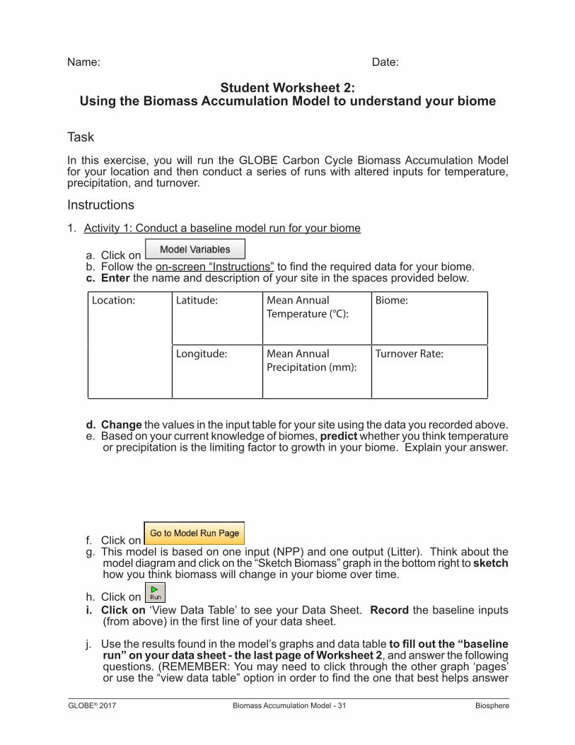
1. Activity 1: Conduct a baseline model run for your biome

a. Click on b. Follow the on-screen “Instructions” to find the required data for your biome.c. Enter the name and description of your site in the spaces provided below.

d. Change the values in the input table for your site using the data you recorded above.e. Based on your current knowledge of biomes, predict whether you think temperature

or precipitation is the limiting factor to growth in your biome. Explain your answer.

I think temperature is the limiting factor to growth in my biome because it gets really cold here in the winter. Because it gets cold many of the trees shed their leaves. I also know that we get precipitation during all of our seasons in New Hampshire.

f. Click on g. This model is based on one input (NPP) and one output (Litter). Think about the

model diagram and click on the “Sketch Biomass” graph in the bottom right to sketch how you think biomass will change in your biome over time.

h. Click on i. Click on ‘View Data Table’ to see your Data Sheet. Record the baseline inputs

(from above) in the first line of your data sheet.

j. Use the results found in the model’s graphs and data table to fill out the “baseline run” on your data sheet, and answer the following questions. (REMEMBER: You may need to click through the other graph ‘pages’ or use the “view data table” option

Location:

MacDonald Lot,Durham, NH

Latitude: 43.13 Mean Annual Temperature (°C):

8.0 °C

Biome: Temperate Broadleaf and Mixed Forest

Longitude: -70.93

Mean Annual Precipitation (mm):

1070.6mm

Turnover Rate: 0.05


in order to find the one that best helps answer the question.)

i. When does vegetation biomass reach equilibrium (aka. year of equilibrium) for the scenario you conducted?

150 years after the start of the simulation

(NOTE: You may need to estimate the time to equilibrium if the model doesn’t run long enough to reach equilibrium on the first try.)

ii. What is the total biomass (g/m2) at the time of equilibrium?

24610g/m2

iii. Earlier you sketched annual biomass accumulation, which is defined as the increase in biomass that occurs in a given year. How does your sketch compare to what actually happened? In general, did biomass increase, decrease or stay the same? What do you think caused this pattern in biomass?

I sketched biomass increasing over the entire 200-year period that the model ran. While biomass did increase initially, the accumulation of biomass slowed down over time and eventually leveled off. The fact that eventually biomass leveled off means that the ecosystem has reached equilibrium. By definition this means that system inputs must equal system outputs. Because in this model we have a constant input (NPP determined by either temperature or precipitation) we must consider how litterfall changed over time in order to understand equilibrium. On page 2 of the upper graph litterfall is shown to have increased from 0 at the start of the simulation to 1231g/m2 by the end of the simulation. Litterfall is tied to the biomass pool, so as the biomass increased, so did the amount of litter produced each year, which explains why the shape of the curves are the same.

This acts like a real system: As an ecosystem matures and the gaps of space between trees were filled in by other trees, shade tolerate trees take hold beneath taller canopies and where some trees die others sprout in their place. Eventually, barring no major disturbance such as logging, insect defoliation, fire, etc., the ecosystem’s death per year will equal its growth.

2. Activity 2: Understand turnover rate

a. Keep precipitation and temperature at baseline values for your site and conduct 4 model runs with altered values of the turnover rate. Select two reasonable values that are lower than your site and two values that are higher. Reasonable values are values you would still expect to occur in your biome, i.e. turnover rate for a temperate biome is 0.05, a reasonable value would be 0.04. Record your results, making sure to also record the inputs you used (record on your data sheet).

*NOTE: you will find a completed data sheet for activities 2 & 3, including graphs in the Biomass Accumulation Worksheet 2 Example Data Sheet (xls available from GLOBE Carbon Cycle webpage).

b. Graph your data from the baseline run (1) and runs 2-5, where precipitation and temperature remained the same but turnover rate was varied. Remember that the variable you are testing (turnover rate in this case) is your independent variable


(x-axis).

i. Graph 1. Turnover rate (x-axis) vs. # of Years to Equilibrium (y-axis)ii. Graph 2. Turnover rate (x-axis) vs. Biomass at Equilibrium (y-axis)

c. What does your data mean? Answer the following questions.

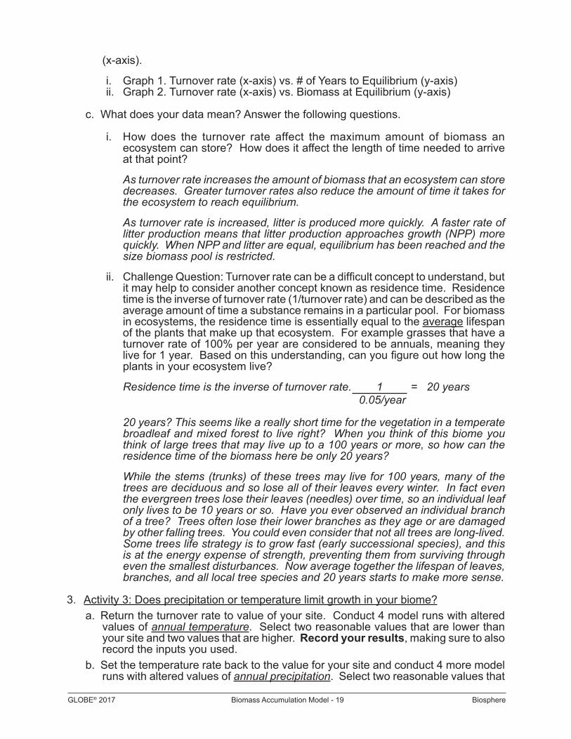
i. How does the turnover rate affect the maximum amount of biomass an ecosystem can store? How does it affect the length of time needed to arrive at that point?

As turnover rate increases the amount of biomass that an ecosystem can store decreases. Greater turnover rates also reduce the amount of time it takes for the ecosystem to reach equilibrium.

As turnover rate is increased, litter is produced more quickly. A faster rate of litter production means that litter production approaches growth (NPP) more quickly. When NPP and litter are equal, equilibrium has been reached and the size biomass pool is restricted.

ii. Challenge Question: Turnover rate can be a difficult concept to understand, but it may help to consider another concept known as residence time. Residence time is the inverse of turnover rate (1/turnover rate) and can be described as the average amount of time a substance remains in a particular pool. For biomass in ecosystems, the residence time is essentially equal to the average lifespan of the plants that make up that ecosystem. For example grasses that have a turnover rate of 100% per year are considered to be annuals, meaning they live for 1 year. Based on this understanding, can you figure out how long the plants in your ecosystem live?

Residence time is the inverse of turnover rate. 1 = 20 years 0.05/year

20 years? This seems like a really short time for the vegetation in a temperate broadleaf and mixed forest to live right? When you think of this biome you think of large trees that may live up to a 100 years or more, so how can the residence time of the biomass here be only 20 years?

While the stems (trunks) of these trees may live for 100 years, many of the trees are deciduous and so lose all of their leaves every winter. In fact even the evergreen trees lose their leaves (needles) over time, so an individual leaf only lives to be 10 years or so. Have you ever observed an individual branch of a tree? Trees often lose their lower branches as they age or are damaged by other falling trees. You could even consider that not all trees are long-lived. Some trees life strategy is to grow fast (early successional species), and this is at the energy expense of strength, preventing them from surviving through even the smallest disturbances. Now average together the lifespan of leaves, branches, and all local tree species and 20 years starts to make more sense.

3. Activity 3: Does precipitation or temperature limit growth in your biome?a. Return the turnover rate to value of your site. Conduct 4 model runs with altered

values of annual temperature. Select two reasonable values that are lower than your site and two values that are higher. Record your results, making sure to also record the inputs you used.

b. Set the temperature rate back to the value for your site and conduct 4 more model runs with altered values of annual precipitation. Select two reasonable values that


are lower than your site and two values that are higher. Record your results, making sure to also record the inputs you used.

c. Graph your data from the baseline run (1) and runs 6-13, where precipitation and temperature were varied and turnover rate remained the same. Remember that the variable you are testing is your independent variable (x-axis).i. Graph 3. Temperature (x-axis) vs. # of Years to Equilibrium (y-axis)ii. Graph 4. Precipitation (x-axis) vs. # of Years to Equilibrium (y-axis)iii. Graph 5. Temperature (x-axis) vs. Biomass at Equilibrium (y-axis)iv. Graph 6. Precipitation (x-axis) vs. Biomass at Equilibrium (y-axis)v. Graph 7. NPP (x-axis) vs. Biomass at Equilibrium (y-axis)vi. Graph 8. # of Years to Equilibrium (x-axis) vs. Biomass at Equilibrium (y-axis)

d. What does your data mean? Answer the following questions using the model’s graphs and table, as well as your own graphs and data sheet.i. How does the time until equilibrium and the biomass at equilibrium change as

temperature and precipitation change?In this biome, a temperate broadleaf and mixed forest, if temperature is altered by a reasonable amount (MAT 6-10°C) both the # of years until equilibrium and the biomass at equilibrium increase with increasing temperature.This was different than the effect of precipitation. As precipitation was altered, neither an increase nor decrease in precipitation from the MAP caused a change in the amount of time the biomass took to reach equilibrium or the maximum amount of biomass at equilibrium.

ii. Which climate variable was predicted by the model to be limiting growth at your site, temperature or precipitation? How do you know this? Was it consistent across trials?Temperature was the limiting factor to growth in my biome and was consistent across all trials of altered temperature and precipitation. I know this for two reasons:1. Because precipitation never affected the number of years to equilibrium

or the maximum biomass at equilibrium during my model runs, and all reasonable values of temperature for my biome did result in different biomass values I can conclude that temperature is the limiting factor to growth in this biome.

2. Because for all trials of altered precipitation and temperature the “model selected NPP” (the NPP chosen by the model to carry out the rest of the model calculations) was the same as the “NPPT” (the NPP predicted using the given temperature). Even using smaller precipitation values the lowest NPPP was greater than the NPPT produced using the greater reasonable temperature values for the biome.

e. Now conduct additional runs using more extreme values of temperature and precipitation. Design your runs to answer the following questions. i. Briefly describe the runs you conducted.ii. How did your limiting factor change under extreme conditions?

Using temperatures significantly lower than those found in my biome resulted in lower NPPT and temperature continued to be the limiting factor to growth.When I used temperatures at least 4 degrees greater than the MAT for my biome I found that the limiting factor changed from temperature to precipitation. Any temperature change greater than that resulted in the same maximum biomass


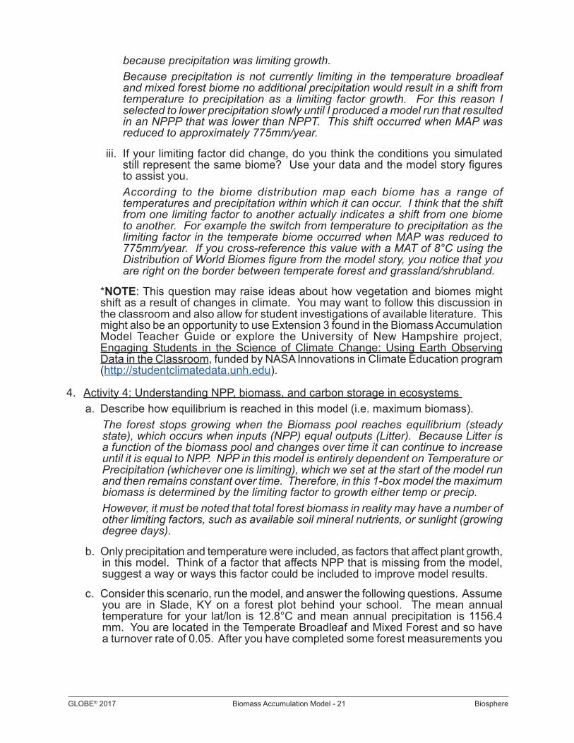
because precipitation was limiting growth.Because precipitation is not currently limiting in the temperature broadleaf and mixed forest biome no additional precipitation would result in a shift from temperature to precipitation as a limiting factor growth. For this reason I selected to lower precipitation slowly until I produced a model run that resulted in an NPPP that was lower than NPPT. This shift occurred when MAP was reduced to approximately 775mm/year.

iii. If your limiting factor did change, do you think the conditions you simulated still represent the same biome? Use your data and the model story figures to assist you. According to the biome distribution map each biome has a range of temperatures and precipitation within which it can occur. I think that the shift from one limiting factor to another actually indicates a shift from one biome to another. For example the switch from temperature to precipitation as the limiting factor in the temperate biome occurred when MAP was reduced to 775mm/year. If you cross-reference this value with a MAT of 8°C using the Distribution of World Biomes figure from the model story, you notice that you are right on the border between temperate forest and grassland/shrubland.

*NOTE: This question may raise ideas about how vegetation and biomes might shift as a result of changes in climate. You may want to follow this discussion in the classroom and also allow for student investigations of available literature. This might also be an opportunity to use Extension 3 found in the Biomass Accumulation Model Teacher Guide or explore the University of New Hampshire project, Engaging Students in the Science of Climate Change: Using Earth Observing Data in the Classroom, funded by NASA Innovations in Climate Education program (http://studentclimatedata.unh.edu).

4. Activity 4: Understanding NPP, biomass, and carbon storage in ecosystems a. Describe how equilibrium is reached in this model (i.e. maximum biomass).

The forest stops growing when the Biomass pool reaches equilibrium (steady state), which occurs when inputs (NPP) equal outputs (Litter). Because Litter is a function of the biomass pool and changes over time it can continue to increase until it is equal to NPP. NPP in this model is entirely dependent on Temperature or Precipitation (whichever one is limiting), which we set at the start of the model run and then remains constant over time. Therefore, in this 1-box model the maximum biomass is determined by the limiting factor to growth either temp or precip. However, it must be noted that total forest biomass in reality may have a number of other limiting factors, such as available soil mineral nutrients, or sunlight (growing degree days).

b. Only precipitation and temperature were included, as factors that affect plant growth, in this model. Think of a factor that affects NPP that is missing from the model, suggest a way or ways this factor could be included to improve model results.

c. Consider this scenario, run the model, and answer the following questions. Assume you are in Slade, KY on a forest plot behind your school. The mean annual temperature for your lat/lon is 12.8°C and mean annual precipitation is 1156.4 mm. You are located in the Temperate Broadleaf and Mixed Forest and so have a turnover rate of 0.05. After you have completed some forest measurements you

http://studentclimatedata.unh.edu


know your current biomass is approximately 22,750g/m2. i. How old is your forest at this time?

24 years oldii. Has your forest reached equilibrium at this time?

No, biomass is still accumulating. Ecosystem growth (NPP) is greater than death (Litter).

iii. Is your forest currently a carbon source to or a carbon sink from the atmosphere? Explain your answer.

Carbon Sink: A carbon reservoir that takes in and stores (sequesters) more carbon than it releases. Carbon sinks can serve to partially offset greenhouse gas emissions. Live trees and plants, for example, absorb carbon dioxide through photosynthesis, release the oxygen and store the carbon. Carbon Source: A reservoir or component of the carbon cycle that releases more carbon than it absorbs. Anthropogenic (human caused) emissions are a source of carbon. Dead trees and plants can also release more carbon than they store, as they decompose and release carbon dioxide back to the atmosphere instead of taking it up through photosynthesis.

Because biomass has not reached equilibrium we know that the forest is continuing to take up carbon through photosynthesis (NPP) and adding it to the total carbon storage. This process indicates that our forest is currently a sink of carbon from the atmosphere.

iv. If your forest has not yet reached equilibrium, how much more carbon could it store than it does now?Current carbon storage: 11,385gC/m2 - Maximum carbon storage: 16,075gC/m2

4,690 more grams of carbon per meter squared could be stored in our forest than what is currently here.

v. How many more years will it take before your forest achieves maximum carbon storage? Current year: 24 - Equilibrium year: 156It will take 132 years from now for this forest to achieve maximum carbon storage barring no change in forest variables.

vi. Brainstorm an example of how your forest might switch from a carbon sink to a carbon source.Even though this modeled forest has no mechanism to switch from a carbon sink or a steady state of carbon flux there are many ways that a real forest could be a source of carbon. A forest would be a source of carbon to the atmosphere in any situation where litter production exceeded growth in a year (i.e. logging harvest, insect outbreak, a major storm-hurricane, ice, flood).


TEACHER VERSION


Student Worksheet 3:Using the Biomass Accumulation Model to Explore Climate Change

*** NOTE: We have provided example answers below. However, student answers to this worksheet are going to vary considerably depending on the biome, climate scenarios, and climate variables they choose to investigate. ***

Task

In this activity you will explore how changes in temperature and precipitation, predicted to occur with climate change, might influence NPP, biomass and/or carbon storage in one or multiple biomes. You will pose a research question, develop an investigation plan, and investigate and analyze model results.

Instructions

1. Activity 1: Develop your research question and hypothesisa. Spend 5-10 minutes exploring the climate maps, animations, and/or the biome

mapper on the Student Climate Data website to identify what location you are interested in investigating.

b. What biome(s) did you select to study?I chose to study the Boreal forests of Canada.

c. Using the temperature and precipitation maps or animations as a resource, how will temperature and precipitation change in the next 100 years in this location?Both temperature and precipitation will increase in this location over the next 100 years

d. Pose a research question that focuses on changes in temperature and precipitation and can be answered using the Biomass Accumulation Model.How does climate change affect biomass accumulation in boreal ecosystems?

e. Write a hypothesis statement that will either be supported or not supported by the model output data. State your hypothesis:As temperature and precipitation increase (due to climate change) in boreal Canada, the biomass accumulation will also increase.

2. Activity 2: Find model inputsa. Open the Biomass Accumulation Model.

b. Click on and then click

c. Follow the instructions to find the latitude/longitude and use the Climate Data tool to find annual climate data for your location of study. Record all values in Table 1.

d. Once you have entered the lat/lon in the Climate Data tool, and the page has finished loading, click ’Table of 30 Year Averages” and select the CO2 climate emission scenario (high, mid, or low) that you are interested in investigating. Record the temperature and precipitation values for that scenario in the table below. (Or create


new tables that better suit your investigation.)

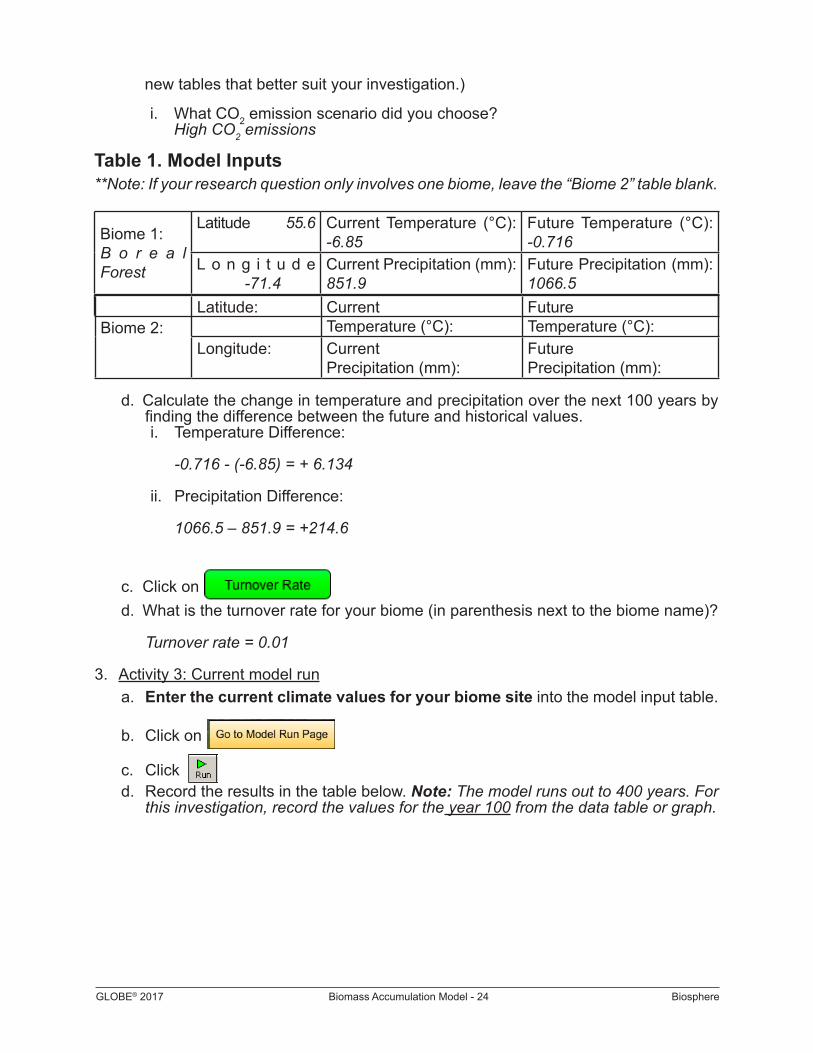
i. What CO2 emission scenario did you choose?High CO2 emissions

Table 1. Model Inputs**Note: If your research question only involves one biome, leave the “Biome 2” table blank.

Biome 1:B o r e a l Forest

Latitude 55.6 Current Temperature (°C): -6.85

Future Temperature (°C): -0.716

L o n g i t u d e -71.4

Current Precipitation (mm): 851.9

Future Precipitation (mm): 1066.5

Biome 2:Latitude: Current

Temperature (°C):Future Temperature (°C):

Longitude: Current Precipitation (mm):

Future Precipitation (mm):

d. Calculate the change in temperature and precipitation over the next 100 years by finding the difference between the future and historical values.i. Temperature Difference:

-0.716 - (-6.85) = + 6.134

ii. Precipitation Difference:

1066.5 – 851.9 = +214.6

c. Click on d. What is the turnover rate for your biome (in parenthesis next to the biome name)?

Turnover rate = 0.01

3. Activity 3: Current model runa. Enter the current climate values for your biome site into the model input table.

b. Click on

c. Click d. Record the results in the table below. Note: The model runs out to 400 years. For

this investigation, record the values for the year 100 from the data table or graph.


BiomePredicted

NPP-T(g/m2yr)

Predicted NPP-P(g/m2yr)

Model Selected

NPP(g/m2yr)

Year of Equilibrium

Biomass at Equilibrium

(g/m2)

Carbon Storage at Equilibrium

BorealForest 326.49 1,296.05 326 N o t

Reached 20,667 10,333.5

Biome

Predicted Final

NPP-T(g/m2yr)

Predicted Final

NPP-P(g/m2yr)

Model Selected

Final NPP(g/m2yr)

Year of Equilibrium


(g/m2)

Carbon Storage at Equilibrium

BorealForest 592.85 1,517.82 590 N o t

Reached 29,767 14,883.5

Table 2. Model Results: Current Run**Note: If equilibrium is not reached in your model run, record the final biomass and carbon storage

4. Activity 4: Future model runa. Do not change the values in the model input table!

b. Click on c. Use the dials to increase or decrease the temperature and precipitation values

using your calculated changes above.d. Run the model and record the results in the table below

Table 3. Model Results: Future Run**Note: If equilibrium is not reached in your model run, record the final biomass and carbon storage

5. Activity 5: Analysis and discussiona. Over the 100-year current model run did biomass reach equilibrium? Did this change

when the model was run under future conditions? If so, how?The model did not reach equilibrium in the current model run or the future model run. In both cases the biomass was still changing at 100 years.

b. What was the difference in total biomass at year 100 between the current and future model runs? At year 100, the biomass was greater in the future run than in current run. Biomass in boreal Canada was 9100 g/m2 greater when the model was run under future


climate conditions than under current climate conditions.

c. Was your hypothesis supported by the data from your model runs? Why or why not?My hypothesis was supported by the data. I hypothesized that biomass accumulation would increase as temperature and precipitation increased with climate change, and the data from the model runs suggest that the biomass was greater when the model was run under future conditions (i.e., increased temperature and precipitation) than when the model was run under current conditions.

d. Develop two new research questions you have after viewing your model results. (These can be beyond the scope of the model.)1. If temperature and precipitation increase in the boreal regions of Canada, will

species composition also change? 2. How would a change in species composition affect the biomass accumulation

in the boreal regions of Canada?

c. What data or information would you need to answer these new questions?For the first research question, I would need information about the species that inhabit boreal Canada, and any information about predicted changes in species composition with climate change. I could use the Tree and Bird Atlases I saw on the Student Climate Data website to get some of this information. For the second research question I could run the biomass accumulation model with the same temperature and precipitation data, but change the turnover rates (i.e. change the biome). In order to choose an appropriate new biome and turnover rate, I would need to get an idea of how the species composition might change in this region (see above) and I would need to find information about the species composition of other biomes.


Name: Date:

Student Worksheet 1:Learning the science behind the Biomass Accumulation Model

Task

In this exercise, you will learn about the science used to build the GLOBE Carbon Cycle Biomass Accumulation model. You should follow the instructions below to record new vocabulary and answer quick questions based on your prior knowledge and understandings gained during the model “story”.

Instructions 1. Open the Biomass Accumulation Model. (In some cases the iSeePlayer needs to be

open first.)

2. To learn about the science of the model, click and read the story. While you read: a. Summarize the definitions of new vocabulary in your own words. Be sure to record

all units.b. Answer quick questions to the best of your ability, you will be assessed on your

thought process.

Activity

Vocabulary 1: Carbon Storage

Vocabulary 2: Carbon Uptake

Vocabulary 3: Biomass

How is biomass related to carbon storage?


Vocabulary 4: Net Primary Productivity (NPP) (also referred to as productivity)

How is NPP related to carbon uptake?

Quick Question 1: What factors influence ecosystem vegetation growth? Locally? Globally?Your answer:

How does your answer compare to the provided answer?

Quick Question 2: Brainstorm where/how you might be able to obtain mean annual temperature and precipitation data. Suggest at least two possible ideas

Quick Question 3: In this model example, which climatic factor (temperature or precipitation) is limiting vegetation growth?

How did you determine your answer?


Vocabulary 5: Litter

Quick Question 4: What factors do you think determine ecosystem litterfall?

What factors are used to determine litterfall in this model?

Vocabulary 6: Turnover Rate

Quick Question 5: Based on your current knowledge, what do you think the turnover rate is for your biome? Provide a range (example: 0.02 - 0.1 or 2% - 10% per year) and explain your reasoning.

Record the turnover rate for your biome.

Quick Question 6: If a turnover rate of 1 means 100% of vegetation turns over in a year, what does a turnover rate of more than 1 mean? When might this be the case?


Activity Summary

Do you have any questions about the model or the system that you are modeling?

Develop a testable research question. (How could this model be used to investigate, your biome, a comparison between biomes, or a connection to field collected data)?

The Biomass Accumulation Model shows how carbon moves to and from the plant pool. To put your work in the context of the global carbon cycle, draw and label the model you are using in this activity. Then add and label two pools to show where carbon comes from and where it goes to after leaving biomass.


Name: Date:

Student Worksheet 2:Using the Biomass Accumulation Model to understand your biome

Task

In this exercise, you will run the GLOBE Carbon Cycle Biomass Accumulation Model for your location and then conduct a series of runs with altered inputs for temperature, precipitation, and turnover.

Instructions

1. Activity 1: Conduct a baseline model run for your biome

a. Click on b. Follow the on-screen “Instructions” to find the required data for your biome.c. Enter the name and description of your site in the spaces provided below.

d. Change the values in the input table for your site using the data you recorded above.e. Based on your current knowledge of biomes, predict whether you think temperature

or precipitation is the limiting factor to growth in your biome. Explain your answer.

f. Click on g. This model is based on one input (NPP) and one output (Litter). Think about the

model diagram and click on the “Sketch Biomass” graph in the bottom right to sketch how you think biomass will change in your biome over time.

h. Click on i. Click on ‘View Data Table’ to see your Data Sheet. Record the baseline inputs

(from above) in the first line of your data sheet.

j. Use the results found in the model’s graphs and data table to fill out the “baseline run” on your data sheet - the last page of Worksheet 2, and answer the following questions. (REMEMBER: You may need to click through the other graph ‘pages’ or use the “view data table” option in order to find the one that best helps answer

Location: Latitude: Mean Annual Temperature (°C):

Biome:

Longitude: Mean Annual Precipitation (mm):

Turnover Rate:


the question.) i. When does vegetation biomass reach equilibrium (aka. year of equilibrium)

for the scenario you conducted? (NOTE: You may need to estimate the time to equilibrium if the model doesn’t run long enough to reach equilibrium on the first try.)

ii. What is the total biomass (g/m2) at the time of equilibrium?

iii. Earlier you sketched annual biomass accumulation, which is defined as the increase in biomass that occurs in a given year. How does your sketch compare to what actually happened? In general, did biomass increase, decrease or stay the same? What do you think caused this pattern in biomass?

2. Activity 2: Understand turnover rate

a. Keep precipitation and temperature at baseline values for your site and conduct 4 model runs with altered values of the turnover rate. Select two reasonable values that are lower than your site and two values that are higher. Reasonable values are values you would still expect to occur in your biome, i.e. turnover rate for a temperate biome is 0.05, a reasonable value would be 0.04. Record your results, making sure to also record the inputs you used (record on your data sheet).

b. On separate paper or in a spreadsheet, graph your data from the baseline run (1) and runs 2-5, where precipitation and temperature remained the same but turnover rate was varied. Remember that the variable you are testing (turnover rate in this case) is your independent variable (x-axis).

i. Graph 1. Turnover rate (x-axis) vs. # of Years to Equilibrium (y-axis)ii. Graph 2. Turnover rate (x-axis) vs. Biomass at Equilibrium (y-axis)

c. What does your data mean? Answer the following questions.

i. How does the turnover rate affect the maximum amount of biomass an ecosystem can store? How does it affect the length of time needed to arrive at that point?

ii. Challenge Question: Turnover rate can be a difficult concept to understand, but it may help to consider another concept known as residence time. Residence time is the inverse of turnover rate (1/turnover rate) and can be described as the average amount of time a substance remains in a particular pool. For biomass in ecosystems, the residence time is essentially equal to the average lifespan of the plants that make up that ecosystem. For example grasses that have a turnover rate of 100% per year are considered to be annuals, meaning


they live for 1 year. Based on this understanding, can you figure out how long the plants in your ecosystem live?

Residence time is the inverse of turnover rate. Ex: 1 = 20 years 0.05/year

3. Activity 3: Does precipitation or temperature limit growth in your biome?a. Return the turnover rate to value of your site. Conduct 4 model runs with altered

values of annual temperature. Select two reasonable values that are lower than your site and two values that are higher. Record your results, making sure to also record the inputs you used.

b. Set the temperature rate back to the value for your site and conduct 4 more model runs with altered values of annual precipitation. Select two reasonable values that are lower than your site and two values that are higher. Record your results, making sure to also record the inputs you used.

c. Graph your data from the baseline run (1) and runs 6-13, where precipitation and temperature were varied and turnover rate remained the same. Remember that the variable you are testing is your independent variable (x-axis).i. Graph 3. Temperature (x-axis) vs. # of Years to Equilibrium (y-axis)ii. Graph 4. Precipitation (x-axis) vs. # of Years to Equilibrium (y-axis)iii. Graph 5. Temperature (x-axis) vs. Biomass at Equilibrium (y-axis)iv. Graph 6. Precipitation (x-axis) vs. Biomass at Equilibrium (y-axis)v. Graph 7. NPP (x-axis) vs. Biomass at Equilibrium (y-axis)vi. Graph 8. # of Years to Equilibrium (x-axis) vs. Biomass at Equilibrium (y-axis)

d. What does your data mean? Answer the following questions using the model’s graphs and table, as well as your own graphs and data sheet.

i. How does the time until equilibrium and the biomass at equilibrium change as temperature and precipitation change?

ii. Which climate variable was predicted by the model to be limiting growth at your site, temperature or precipitation? How do you know this? Was it consistent across trials?


e. Now conduct additional runs using more extreme values of temperature and precipitation. Design your runs to answer the following questions. i. Briefly describe the runs you conducted.

ii. How did your limiting factor change under extreme conditions?

iii. If your limiting factor did change, do you think the conditions you simulated still represent the same biome? Use your data and the model story figures to assist you.

4. Activity 4: Understanding NPP, biomass, and carbon storage in ecosystems a. Describe how equilibrium is reached in this model (i.e. maximum biomass).b. Only precipitation and temperature were included, as factors that affect plant growth,

in this model. Think of a factor that affects NPP that is missing from the model, suggest a way or ways this factor could be included to improve model results.

c. Consider this scenario, run the model, and answer the following questions. Assume you are in Slade, KY on a forest plot behind your school. The mean annual temperature for your lat/lon is 12.8°C and mean annual precipitation is 1156.4mm. You are located in the Temperate Broadleaf and Mixed Forest and so have a turnover rate of 0.05. After you have completed some forest measurements you know your current biomass is approximately 22,750g/m2.

i. How old is your forest at this time?


current biomass is approximately 22,750g/m2. iv. Has your forest reached equilibrium at this time?

v. Two vocabulary terms scientists often use when discussing carbon in ecosystems are sink and source:

Carbon Sink: A carbon reservoir that takes in and stores (sequesters) more carbon than it releases. Carbon sinks can serve to partially offset greenhouse gas emissions. Live trees and plants, for example, absorb carbon dioxide through photosynthesis, release the oxygen and store the carbon. Carbon Source: A reservoir or component of the carbon cycle that releases more carbon than it absorbs. Anthropogenic (human caused) emissions are a source of carbon. Dead trees and plants can also release more carbon than they store, as they decompose and release carbon dioxide back to the atmosphere instead of taking it up through photosynthesis.

In this scenario, is your forest currently a carbon source to or a carbon sink from the atmosphere? Explain your answer.

vi. If your forest has not yet reached equilibrium, how much more carbon could it store than it does now?

vii. How many more years will it take before your forest achieves maximum carbon storage?

viii. Brainstorm an example of how your forest might switch from a carbon sink to a carbon source.


# Altered Variable

MeanAnnualTemp

(Celsius)

MeanAnnualPrecip.(mm)

TurnoverRate (per

year)

PredictedNPP-T

(g/m2y)

PredictedNPP-P

(g/m2y)

Model Selected

NPP(g/m2y)

Years to Equilibrium


(g/m2)

1 Baseline Run

2 Turnover Rate

3 Turnover Rate

4 Turnover Rate

5 Turnover Rate

6 Baseline Run

7 Temp

8 Temp

9 Temp

10 Temp

11 Baseline Run

12 Precip

13 Precip

14 Precip

15 Precip

16

17

18

19

20

21

22


Name: Date:

Student Worksheet 3 Extension:Using the Biomass Accumulation Model to Explore Climate Change

Task

In this activity you will explore how changes in temperature and precipitation, predicted to occur with climate change, might influence NPP, biomass and/or carbon storage in one or multiple biomes. You will pose a research question, develop an investigation plan, and investigate and analyze model results.

Instructions

1. Activity 1: Develop your research question and hypothesisa. Spend 5-10 minutes exploring the climate maps, animations, and/or the biome

mapper on the Student Climate Data website to identify what location you are interested in investigating.

b. What biome(s) did you select to study?

c. Using the temperature and precipitation maps or animations as a resource, how will temperature and precipitation change in the next 100 years in this location?

d. Pose a research question that focuses on changes in temperature and precipitation and can be answered using the Biomass Accumulation Model.

e. Write a hypothesis statement that will either be supported or not supported by the model output data. State your hypothesis:

2. Activity 2: Find model inputsa. Open the Biomass Accumulation Model.

b. Click on and then click

c. Follow the instructions to find the latitude/longitude and use the Climate Data tool to find annual climate date for your location of study. Record all values in Table 1.

d. Once you have entered the lat/lon in the Climate Data tool, and the page has finished


loading, click ’Table of 30 Year Averages” and select the CO2 climate emission scenario (high, mid, or low) that you are interested in investigating. Record the temperature and precipitation values for that scenario in the table below. (Or create new tables that better suit your investigation.)

i. What CO2 emission scenario did you choose?

Table 1. Model Inputs**Note: If your research question only involves one biome, leave the “Biome 2” table blank.

Biome 1:Latitude: Current Temperature (°C): Future Temperature (°C):

Longitude: Current Precipitation (mm): Future Precipitation (mm):

Biome 2:Latitude: Current

Temperature (°C):Future Temperature (°C):

Longitude: Current Precipitation (mm):

Future Precipitation (mm):

d. Calculate the change in temperature and precipitation over the next 100 years by finding the difference between the future and historical values.i. Temperature Difference:

ii. Precipitation Difference:

c. Click on d. What is the turnover rate for your biome (in parenthesis next to the biome name)?

3. Activity 3: Current model runa. Enter the current climate values for your biome site into the model input table.

b. Click on

c. Click

d. Record the results in Table 2. Note: The model runs out to 400 years. For this investigation, record the values for the year 100 from the data table or graph.


Table 2. Model Results: Current Run**Note: If equilibrium is not reached in your model run, record the final biomass and carbon storage

BiomePredicted

NPP-T(g/m2yr)

Predicted NPP-P

(g/m2yr)

Model Selected

NPP(g/m2yr)

Year of Equilibrium


(g/m2)

Carbon Storage at

Equilibrium

4. Activity 4: Future model runa. Do not change the values in the model input table!

b. Click on

c. Use the dials to increase or decrease the temperature and precipitation values using your calculated changes on the previous page.

d. Run the model and record the results in Table 3.

Table 3. Model Results: Future Run**Note: If equilibrium is not reached in your model run, record the final biomass and carbon storage

BiomePredicted

Final NPP-T(g/m2yr)

Predicted Final NPP-P

(g/m2yr)

Model Selected Final NPP(g/m2yr)

Year of Equilibrium


(g/m2)

Carbon Storage at

Equilibrium

5. Activity 5: Analysis and discussiona. Over the 100-year ‘current’ model run did biomass reach equilibrium? Did this

change when the model was run under future conditions? If so, how?


b. What was the difference in total biomass at year 100 between the current and future model runs?

c. Was your hypothesis supported by the data from your model runs? Why or why not?

d. Develop two new research questions you have after viewing your model results. (These can be beyond the scope of the model.)

e. What data or information would you need to answer these new questions?

biomass accumulation model - globe.gov

Documents