BIOLOGICALLY INSPIRED APPROACH FOR ROBOT DESIGN AND CONTROL

By

Jianguo Zhao

A DISSERTATION

Submitted toMichigan State University

in partial fulfillment of the requirementsfor the degree of

Electrical Engineering - Doctor of Philosophy

2015

ABSTRACT

BIOLOGICALLY INSPIRED APPROACH FOR ROBOT DESIGN AND CONTROL

By

Jianguo Zhao

Robots will transform our daily lives in the near future by moving from controlled in-

dustrial lines to unstructured and uncertain environments such as home, offices, or outdoors

with various applications from healthcare, service, to defense. Nevertheless, two fundamen-

tal problems remain unsolved for robots to work in such environments. On one hand, how

to design robots, especially meso-scale ones with sizes of a few centimeters, with multiple

locomotion abilities to travel in the unstructured environment is still a daunting task. On

the other hand, how to control such robots to dynamically interact with the uncertain envi-

ronment for agile and robust locomotion also requires tremendous efforts. This dissertation

tries to tackle these two problems in the framework of biologically inspired robotics.

On the design aspect, it will be shown how biologically principles found in nature can be

used to build efficient meso-scale robots with various locomotion abilities such as jumping,

wheeling, and aerial maneuvering. Specifically, a robot (MSU Jumper) with continuous

jumping ability will be presented. The robot can achieve the following three performances

simultaneously. First, it can perform continuous steerable jumping based on the self-righting

and the steering capabilities. Second, the robot only requires a single actuator to perform all

the functions. Third, the robot has a light weight (23.5 g) to reduce the damage from landing

impacts. Based on the MSU Jumper, a robot (MSU Tailbot) with multiple locomotion

abilities is discussed. This robot can not only wheel on the ground but also jump up to

overcome obstacles. Once leaping into the air, it can also control its body angle using an

active tail to dynamically maneuver in mid-air for safe landings.

On the control aspect, a novel non-vector space control method that formulates the

problem in the space of sets is presented. This method can be easily applied to vision based

control by considering images as sets. The advantage of such a method is that there is no

need to extract and track features during the control process, which is required by traditional

methods. Based on the non-vector space approach, the compressive feedback is proposed to

increase the feedback rate and reduce the computation time. This method is ideal for the

control of meso-scale robots with limited sensing and computation ability.

The bio-inspired design illustrated by the MSU Jumper and MSU Tailbot in this disser-

tation can be applied to other robot designs. Meanwhile, the non-vector space control with

compressive feedbacks lays the foundation for the control of high dynamic meso-scale robots.

Together, the biologically inspired method for the design and control of meso-scale robots

will pave the way for next generation bio-inspired, low cost, and agile robots.

ACKNOWLEDGMENTS

First and foremost, I would like to thank and express my great appreciation and gratitude

to my advisor Dr. Ning Xi. Without his support, I would not be able to initiate my PhD

study in US. Moreover, without his guidance, it was impossible for me to finish the research

presented this dissertation. His insightful vision and high standard for research also made

me a qualified researcher.

I would like to thank my dissertation committee members: Dr. Xiaobo Tan, Dr. Matt

W Mutka, Dr. Li Xiao, and Dr. Hassan Khalil. I greatly appreciate their valuable feedback

and discussions throughout my entire PhD process.

My many thanks go to my lab members: Dr. Yunyi Jia, Yu Cheng, Bo Song, Liangliang

Chen, Dr. Ruiguo Yang, Dr. Erick Nieves, Dr. Hongzhi Chen, Dr. Chi Zhang, Dr. Yong

Liu, Dr. Bingtuan Gao, Dr. Jing Xu, Dr. King W.C. Lai, Dr. Carmen K.M. Fung, and

Dr. Yongliang Yang. I was fortunate to collaborate with many of them for various projects

which widely broadened my view. Many professors spent their time as visiting scholars in

our lab in the past few years. I want to thank them for many extracurricular activities,

which provide many joys besides research.

I would also like to thank undergraduate students who worked with me on various parts

of this dissertation. Among them are Tianyu Zhao, Chenli Yuan, Weihan Yan, Hongyi Shen,

and Zach Farmer. By working with them, I also gained experiences on how to supervise

students for various projects.

Finally, I thank my parents and my wife for their endurance and support for such a long

commitment for the PhD study.

iv

TABLE OF CONTENTS

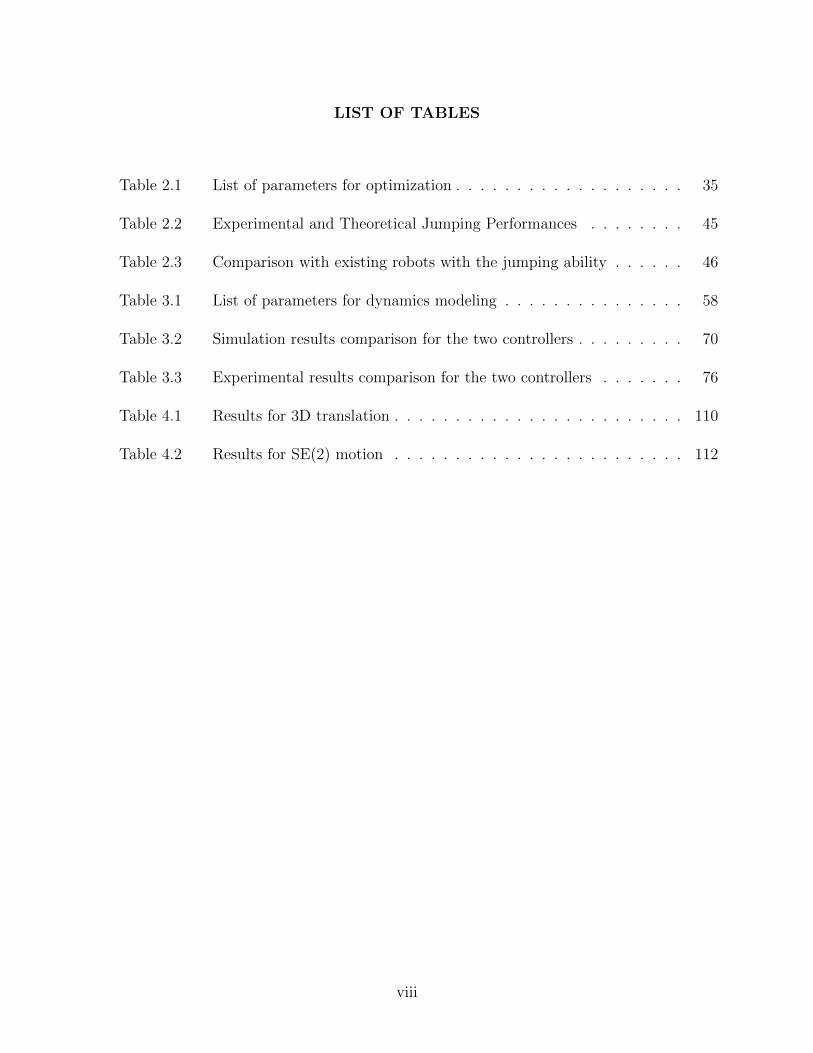
LIST OF TABLES . . . . . . . . . . . . . . . . . . . . . . . . . . . . . . . . . . . . viii

LIST OF FIGURES . . . . . . . . . . . . . . . . . . . . . . . . . . . . . . . . . . . ix

Chapter 1 Introduction . . . . . . . . . . . . . . . . . . . . . . . . . . . . . . . 11.1 Background . . . . . . . . . . . . . . . . . . . . . . . . . . . . . . . . . . . . 11.2 Challenges and Objectives . . . . . . . . . . . . . . . . . . . . . . . . . . . . 31.3 Literature Review . . . . . . . . . . . . . . . . . . . . . . . . . . . . . . . . . 6

1.3.1 Biological Inspired Robot Locomotion . . . . . . . . . . . . . . . . . 61.3.2 Biological Inspired Robot Control . . . . . . . . . . . . . . . . . . . . 10

1.4 Contributions . . . . . . . . . . . . . . . . . . . . . . . . . . . . . . . . . . . 121.5 Outline of This Dissertation . . . . . . . . . . . . . . . . . . . . . . . . . . . 14

Chapter 2 MSU Jumper: A Biologically Inspired Jumping Robot . . . . . 162.1 Introduction . . . . . . . . . . . . . . . . . . . . . . . . . . . . . . . . . . . . 162.2 Modeling of the Jumping Process . . . . . . . . . . . . . . . . . . . . . . . . 202.3 Mechanical Design and Analysis . . . . . . . . . . . . . . . . . . . . . . . . . 24

2.3.1 Jumping Mechanism . . . . . . . . . . . . . . . . . . . . . . . . . . . 242.3.2 Energy Mechanism . . . . . . . . . . . . . . . . . . . . . . . . . . . . 282.3.3 Self-righting Mechanism . . . . . . . . . . . . . . . . . . . . . . . . . 312.3.4 Steering Mechanism . . . . . . . . . . . . . . . . . . . . . . . . . . . 33

2.4 Design Optimization . . . . . . . . . . . . . . . . . . . . . . . . . . . . . . . 342.4.1 Jumping Mechanism and Energy Mechanism . . . . . . . . . . . . . . 352.4.2 Self-righting Mechanism . . . . . . . . . . . . . . . . . . . . . . . . . 39

2.5 Fabrication and Experimental Results . . . . . . . . . . . . . . . . . . . . . . 412.5.1 Fabrication and Development . . . . . . . . . . . . . . . . . . . . . . 412.5.2 Experimental Results . . . . . . . . . . . . . . . . . . . . . . . . . . . 432.5.3 Comparison with Other Robots . . . . . . . . . . . . . . . . . . . . . 47

2.6 Conclusions . . . . . . . . . . . . . . . . . . . . . . . . . . . . . . . . . . . . 49

Chapter 3 MSU Tailbot: A Biologically Inspired Tailed Robot . . . . . . . 503.1 Introduction . . . . . . . . . . . . . . . . . . . . . . . . . . . . . . . . . . . . 503.2 Robot Design . . . . . . . . . . . . . . . . . . . . . . . . . . . . . . . . . . . 52

3.2.1 Mechanical Design . . . . . . . . . . . . . . . . . . . . . . . . . . . . 523.2.2 Electrical Design . . . . . . . . . . . . . . . . . . . . . . . . . . . . . 55

3.3 Dynamics Model and Tail Optimization . . . . . . . . . . . . . . . . . . . . . 573.3.1 Dynamics Model . . . . . . . . . . . . . . . . . . . . . . . . . . . . . 573.3.2 Tail Optimization . . . . . . . . . . . . . . . . . . . . . . . . . . . . . 63

3.4 Controller Design . . . . . . . . . . . . . . . . . . . . . . . . . . . . . . . . . 65

v

3.4.1 Sliding Mode Controller . . . . . . . . . . . . . . . . . . . . . . . . . 663.4.2 Proportional-Derivative (PD) Controller . . . . . . . . . . . . . . . . 68

3.5 Testing Results . . . . . . . . . . . . . . . . . . . . . . . . . . . . . . . . . . 693.5.1 Simulation Results for Aerial Maneuvering . . . . . . . . . . . . . . . 693.5.2 Experimental Results for Aerial Maneuvering . . . . . . . . . . . . . 71

3.5.2.1 Jumping without Tail Actuation . . . . . . . . . . . . . . . 723.5.2.2 Aerial Maneuvering with the PD Controller . . . . . . . . . 733.5.2.3 Aerial Maneuvering with the Sliding Mode Controller . . . . 753.5.2.4 Comparison of the Two Controllers . . . . . . . . . . . . . . 76

3.5.3 Tail Assisted Mode Transition . . . . . . . . . . . . . . . . . . . . . . 763.5.3.1 Wheeling and Turning . . . . . . . . . . . . . . . . . . . . . 77

3.6 Conclusions . . . . . . . . . . . . . . . . . . . . . . . . . . . . . . . . . . . . 78

Chapter 4 Non-vector Space Control: A Biologically Inspired ControlApproach . . . . . . . . . . . . . . . . . . . . . . . . . . . . . . . . . . 85

4.1 Introduction . . . . . . . . . . . . . . . . . . . . . . . . . . . . . . . . . . . . 854.2 Dynamics in the Non-vector Space . . . . . . . . . . . . . . . . . . . . . . . 89

4.2.1 Transitions . . . . . . . . . . . . . . . . . . . . . . . . . . . . . . . . 914.2.2 Mutation Equations . . . . . . . . . . . . . . . . . . . . . . . . . . . 93

4.3 Stabilization Control in the Non-vector Space . . . . . . . . . . . . . . . . . 954.3.1 Stabilization Problem . . . . . . . . . . . . . . . . . . . . . . . . . . . 964.3.2 Lyapunov Function Based Stability Analysis . . . . . . . . . . . . . . 974.3.3 Stabilizing Controller Design . . . . . . . . . . . . . . . . . . . . . . . 100

4.4 Application to Visual Servoing . . . . . . . . . . . . . . . . . . . . . . . . . . 1024.4.1 3D Translation . . . . . . . . . . . . . . . . . . . . . . . . . . . . . . 1044.4.2 SE(2) Motion . . . . . . . . . . . . . . . . . . . . . . . . . . . . . . . 105

4.5 Testing Results . . . . . . . . . . . . . . . . . . . . . . . . . . . . . . . . . . 1054.5.1 3D Translational Motion . . . . . . . . . . . . . . . . . . . . . . . . . 1094.5.2 SE(2) Motion . . . . . . . . . . . . . . . . . . . . . . . . . . . . . . . 111

4.6 Conclusions . . . . . . . . . . . . . . . . . . . . . . . . . . . . . . . . . . . . 112

Chapter 5 Compressive Feedback based Non-vector Space Control . . . . 1135.1 Introduction . . . . . . . . . . . . . . . . . . . . . . . . . . . . . . . . . . . . 1135.2 Mathematical Preliminaries . . . . . . . . . . . . . . . . . . . . . . . . . . . 1155.3 Stabilizing Controller Design . . . . . . . . . . . . . . . . . . . . . . . . . . . 118

5.3.1 Controller Design with Full Feedback . . . . . . . . . . . . . . . . . . 1185.3.2 Controller Design with Compressive Feedback . . . . . . . . . . . . . 119

5.4 Stability Analysis with Compressive Feedback . . . . . . . . . . . . . . . . . 1225.4.1 Stability for Sparse Feedback . . . . . . . . . . . . . . . . . . . . . . 1225.4.2 Stability for Approximate Sparse Feedback . . . . . . . . . . . . . . . 124

5.5 Testing Results . . . . . . . . . . . . . . . . . . . . . . . . . . . . . . . . . . 1275.5.1 3D Translational Motion . . . . . . . . . . . . . . . . . . . . . . . . . 1285.5.2 SE(2) Motion . . . . . . . . . . . . . . . . . . . . . . . . . . . . . . . 129

5.6 Conclusions . . . . . . . . . . . . . . . . . . . . . . . . . . . . . . . . . . . . 131

vi

Chapter 6 Non-vector Space Landing Control for MSU Tailbot . . . . . . 1326.1 Introduction . . . . . . . . . . . . . . . . . . . . . . . . . . . . . . . . . . . . 1326.2 System Description . . . . . . . . . . . . . . . . . . . . . . . . . . . . . . . . 1336.3 Experimental Setup and Results . . . . . . . . . . . . . . . . . . . . . . . . . 1376.4 Conclusions . . . . . . . . . . . . . . . . . . . . . . . . . . . . . . . . . . . . 142

Chapter 7 Conclusions and Future Work . . . . . . . . . . . . . . . . . . . . 1437.1 Conclusions . . . . . . . . . . . . . . . . . . . . . . . . . . . . . . . . . . . . 1437.2 Future Research Work . . . . . . . . . . . . . . . . . . . . . . . . . . . . . . 144

REFERENCES . . . . . . . . . . . . . . . . . . . . . . . . . . . . . . . . 147

vii

LIST OF TABLES

Table 2.1 List of parameters for optimization . . . . . . . . . . . . . . . . . . . 35

Table 2.2 Experimental and Theoretical Jumping Performances . . . . . . . . 45

Table 2.3 Comparison with existing robots with the jumping ability . . . . . . 46

Table 3.1 List of parameters for dynamics modeling . . . . . . . . . . . . . . . 58

Table 3.2 Simulation results comparison for the two controllers . . . . . . . . . 70

Table 3.3 Experimental results comparison for the two controllers . . . . . . . 76

Table 4.1 Results for 3D translation . . . . . . . . . . . . . . . . . . . . . . . . 110

Table 4.2 Results for SE(2) motion . . . . . . . . . . . . . . . . . . . . . . . . 112

viii

LIST OF FIGURES

Figure 1.1 Existing jumping robots based on traditional springs: (a) the firstgeneration of frogbot [1]; (b) the second generation of frogbot [1]; (c)the old surveillance robot [2]; (d) the new surveillance robot [3]; (e)the intermittent hopping robot [4]; (f) the MiniWhegs [5]; (g) theold Grillo robot [6]; (h) the new Grillo robot [7]; (i) the wheel-basedstair-climbing robot [8]; (j) the EPFL jumper V1 [9]; (k) the EPFLjumper V2 [10]; (l) the EPFL jumper V3 [11]; (m) the multimodalrobot [12]; (n) the first generation MSU jumper [13]; (o) the secondgeneration MSU jumper [14]. . . . . . . . . . . . . . . . . . . . . . 8

Figure 1.2 Existing jumping robots based on customized springs: (a) the scoutrobot [15]; (b) the compact jumping robot [16]; (c) the MIT mi-crobot [17]; (d) the Jollbot [18]; (e) the deformable robot [19]; (f) theflea robot [20]. . . . . . . . . . . . . . . . . . . . . . . . . . . . . . 9

Figure 1.3 Existing jumping robots based on compressed air: (a) the old rescuerobot [21]; (b) the new rescue robot [22]; (c) the patrol robot [23];(d) the quadruped Airhopper [24]; (e) the Mowgli robot [25]. . . . . 9

Figure 1.4 Other existing jumping robots: (a) the pendulum jumping machine [26];(b) the old sand flea [27]; (c) the new sand flea [28]; (d) the jumpingmicrorobot [29]; (e) the voice coil based jumper [30]. . . . . . . . . 9

Figure 2.1 MSU jumper: (a) prototype; (b) solid model. . . . . . . . . . . . . . 18

Figure 2.2 Jumping motion sequence with the corresponding motor rotation di-rections. . . . . . . . . . . . . . . . . . . . . . . . . . . . . . . . . . 18

Figure 2.3 Jumping principle for spring based jumping robots. . . . . . . . . . 21

Figure 2.4 Theoretical jumping trajectories for different take-off angles. . . . . 23

Figure 2.5 Jumping mechanism synthesis. . . . . . . . . . . . . . . . . . . . . . 25

Figure 2.6 Schematic of the jumping mechanism: (a) jumping mechanism; (b)static analysis for the right side part. . . . . . . . . . . . . . . . . . 26

Figure 2.7 Illustration of the energy mechanism: (a) intermediate position dur-ing the charge of energy; (b) critical position; (c) intermediate posi-tion during the release of energy. . . . . . . . . . . . . . . . . . . . . 29

ix

Figure 2.8 Statics for the energy mechanism. . . . . . . . . . . . . . . . . . . . 30

Figure 2.9 Illustration of the self-righting mechanism: (a) initial position afterthe robot lands on the ground; (b) final position when the robotstands up. . . . . . . . . . . . . . . . . . . . . . . . . . . . . . . . . 32

Figure 2.10 Details of the self-righting mechanism. . . . . . . . . . . . . . . . . . 32

Figure 2.11 Illustration of the steering mechanism: (a) front view; (b) side view. 34

Figure 2.12 Objective function varies with optimization variables: (a) variationof g(lb, ld, l2, l3) with fixed l2 and l3; (b) variation of g(lb, ld, l2, l3)with fixed lb and ld. . . . . . . . . . . . . . . . . . . . . . . . . . . . 38

Figure 2.13 Torque profile with the optimal dimensions. . . . . . . . . . . . . . . 38

Figure 2.14 Dimension design of the self-righting mechanism: (a) mechanism withinitial and final positions for both self-righting legs; (b) simplificationof the mechanism to determine the length for link AC. . . . . . . . . 40

Figure 2.15 Solid model for each mechanism (a) jumping mechanism (principleshown in Fig. 2.6(a)); (b) energy mechanism (principle shown inFig. 2.7); (c) self-righting mechanism (principle shown in Fig. 2.10);(d) steering mechanism (principle shown in Fig. 2.11). . . . . . . . . 41

Figure 2.16 Jumping experimental results: average trajectories for three sets ofexperiments. . . . . . . . . . . . . . . . . . . . . . . . . . . . . . . . 44

Figure 2.17 Self-righting experimental result: six individual frames extracted froma self-righting video. . . . . . . . . . . . . . . . . . . . . . . . . . . . 45

Figure 2.18 Steering experimental result: four individual frames extracted froma steering video. . . . . . . . . . . . . . . . . . . . . . . . . . . . . . 47

Figure 3.1 The robot motion cycle with the robot prototype in the center. . . . 51

Figure 3.2 Mechanical design of the tailbot: (a) Left view with height and width,and the robot is divided into the body and tail part encircled by tworectangles; (b) Front view with length, and two major parts encircledby two rectangles are shown in (c) and (d), respectively; (c) Sectionview of the tail part; (d) Section view of the gear train part for theenergy mechanism; (e) Working principle of the jumping mechanism;(f) Working principle of the energy mechanism. . . . . . . . . . . . 54

Figure 3.3 The architecture of the embedded control system. . . . . . . . . . . 56

x

Figure 3.4 The schematic of the tailbot in mid-air for dynamics modeling, wherethe body and the tail are connected by a revolute joint at point C(Fig. 3.2(a) shows the tail and body part with solid models). . . . . 58

Figure 3.5 Aerial maneuvering results from video frames show the robot trajec-tory in a single image for three cases. A schematic view for each robotin all the three images is added for illustration purposes. The dashedlines represent the tail, while the solid lines represent the body. (a)the tail is not actuated; (b) the tail is controlled by the PD controller;(c) the tail is controlled by the sliding mode controller. Note that therobot jumps from right to left in the figure. . . . . . . . . . . . . . . 69

Figure 3.6 Simulation results for the PD controller and the sliding mode con-troller. Each curve shows the trajectory for θb with resect to time foreach controller. . . . . . . . . . . . . . . . . . . . . . . . . . . . . . . 71

Figure 3.7 Experimental results for aerial maneuvering when the tail is not actu-ated: (a) the body’s pitch angle with respect to time; (b) the body’sroll angle with respect to time; (c) the body’s yaw angle with respectto time. . . . . . . . . . . . . . . . . . . . . . . . . . . . . . . . . . . 80

Figure 3.8 Experimental results for aerial maneuvering when the tail is con-trolled by the PD controller: (a) the body’s pitch angle with respectto time; (b) the body’s roll angle with respect to time; (c) the body’syaw angle with respect to time. . . . . . . . . . . . . . . . . . . . . . 81

Figure 3.9 Experimental results for aerial maneuvering when the tail is con-trolled by the sliding mode controller: (a) the body’s pitch anglewith respect to time; (b) the body’s roll angle with respect to time;(c) the body’s yaw angle with respect to time. . . . . . . . . . . . . 82

Figure 3.10 Experimental results comparison for the PD controller and the slid-ing mode controller. The two curves are obtained by averaging thetrajectories of five jumps for each controller. . . . . . . . . . . . . . 83

Figure 3.11 Experimental results for transition from wheeling mode to jumpingmode. . . . . . . . . . . . . . . . . . . . . . . . . . . . . . . . . . . . 83

Figure 3.12 Experimental results for transition from jumping mode to wheelingmode. . . . . . . . . . . . . . . . . . . . . . . . . . . . . . . . . . . . 83

Figure 3.13 Running and turning experiments: (a) running experimental resultsand (b) turning experimental results. . . . . . . . . . . . . . . . . . 84

xi

Figure 4.1 Motivation for vision based robot control: (a) bees can land on anarbitrary surface using vision feedback; (b) how can robots, withsimilar feedback mechanism, achieve the same feat? . . . . . . . . . 86

Figure 4.2 Schematic for non-vector space control with the tailbot as an example 88

Figure 4.3 Illustration of the transition set . . . . . . . . . . . . . . . . . . . . 92

Figure 4.4 The implementation framework to verify the non-vector space controller106

Figure 4.5 Experimental setup to verify the non-vector space controller . . . . . 109

Figure 4.6 Initial and desired image for the 3D translation . . . . . . . . . . . . 110

Figure 4.7 Experimental results for the 3D translation . . . . . . . . . . . . . . 110

Figure 4.8 Initial and desired image for the SE(2) motion . . . . . . . . . . . . 111

Figure 4.9 Experimental results for the SE(2) motion . . . . . . . . . . . . . . 111

Figure 5.1 Schematic for non-vector space control with compressive feedback . 114

Figure 5.2 The initial and goal images for the three dimensional translationalmotion experiment. . . . . . . . . . . . . . . . . . . . . . . . . . . . 128

Figure 5.3 Task space errors for the three dimensional translational motion ex-periment. . . . . . . . . . . . . . . . . . . . . . . . . . . . . . . . . . 129

Figure 5.4 The initial and goal images for the SE(2) motion experiment. . . . . 130

Figure 5.5 Task space errors for the SE(2) motion experiment. . . . . . . . . . 131

Figure 6.1 The robot prototype for experiments . . . . . . . . . . . . . . . . . . 133

Figure 6.2 The schematic of the embedded control system . . . . . . . . . . . . 134

Figure 6.3 The illustrated experimental setup of the tailed robot system . . . . 136

Figure 6.4 The experimental setup for implementing the non-vector space con-trol on the tailed robot system . . . . . . . . . . . . . . . . . . . . . 140

Figure 6.5 Images for the landing control experiment: (a) 1st image; (b) 2ndimage; (c) 3rd image; (d) 4th image, (e) 5th image; (f) desired image. 141

xii

Figure 6.6 The value for the Lyapunov function decreases during the controlprocess. . . . . . . . . . . . . . . . . . . . . . . . . . . . . . . . . . . 142

xiii

Chapter 1

Introduction

1.1 Background

Animals employ various methods to move in different environments. On land, worms and

snakes can crawl or burrow, frogs and flea can hop or jump, horses and cheetah can walk or

run. In addition, squirrels can climb on vertical tree trunks, while geckoes can even run on

ceilings. In the air, birds can glide without flapping their wings or soar for sustained gliding

with the use of air movements. Many insects such as bees and hummingbirds can hover to

stay stationary. And of course birds and insects can fly elegantly by flapping their wings.

In water, most fish can swim by undulation. Some of them such as scallops and squids can

swim by jet propulsion. Besides, some insects such as water striders and fish spiders can

move on the surface of water by surface tension force [31].

Recently, many robotic systems have been built based on how animals move, which is

termed as biologically inspired robots [32, 33]. Such robots have similar locomotion abilities

found in animals such as climbing robots, fish robots, flying robots, walking robots, and

jumping robots. Among them, meso-scale robots with sizes of a few centimeters are very

attractive because they have several advantages compared with large size bio-inspired robots.

First, due to their small size, they only have a small number of components. Therefore, they

can be built with a low cost by using current fabrication technology such as 3D printing.

Second, they can access narrow environments where large robots cannot go. Third, also due

1

to their small sizes, they are not noticeable which makes them ideal platforms for applications

such as military surveillance.

With the advantages for meso-scale robots, they can be used for many applications. A

particular example is search and rescue. In natural disasters such as earthquakes, many

victims are trapped under the disaster site. However, it would be dangerous to directly send

humans to search those survivors. In this case, many low cost small robots can be thrown into

the area from aerial or terrestrial vehicles. With multiple locomotion capabilities, they can

move around in the area. With various sensors such as cameras, they can also cooperatively

search the area and locate the position of survivors. Based on the information provided by

them, we can rescue those survivors more effectively and safely.

Besides search and rescue, many other applications also exist. These small robots can

be used for mobile sensor nodes to form mobile sensor networks, which can be used for

environmental monitoring and surveillance. They are especially suitable platforms to verify

and study cooperative control of many robots due to their low costs. With their repeatable

locomotion capability, they can also be used for experiments to test fundamental biological

hypothesis when it is impossible or not reliable to use animals for those experiments. For ex-

ample, Chen, Zhang, and Goldman used small legged robots to investigate how small animals

can locomote in granular media such as sands and proposed the theory of terradynamics [34].

Due to their advantages and applications, many meso-scale robots have been built in the

last decade. For example, the Biomimimetic Millisystems Lab has built several meso-scale

terrestrial robots. DASH is a 16 gram hexapedal robot that can run fast and still work after

fall from a 10m height [35]. MEDIC, also a hexapedal robot, can overcome obstacles [36].

OctoRoACH can use a tail for dynamic and fast turning [37]. VelociRoACH can run at a

very fast speed (2.7 m/s) by considering the aerodynamic effect [38].

2

Besides the meso-scale terrestrial robots, many other robots of similar sizes have been

built as well. The robobee built by the Microrobotics group at Harvard University is a

particular example [39]. The 100 mg robot that can fly with an external power supply [40] is

fabricated by a novel manufacturing method called pop-up book MEMS [41]. Small robots

that are used to study the swarm behavior of many robots are also developed such as the

Kilobot which is a low cost robot system [42].

1.2 Challenges and Objectives

Centimeter scale robots discussed in the previous section will locomote in natural environ-

ments. Since natural environments are unstructured and uncertain, these robots should

satisfy two basic requirements in order for successful locomotion in such environments. On

one hand, due to their small size, there is no single universal and energy efficient locomo-

tion method for unstructured environments. Therefore, these robots should have multiple

locomotion methods or multi-mode locomotion. On the other hand, they should be able

to dynamically interact with uncertain environments to respond to different situations. In

this case, real time onboard control with sensing, computation, and control capabilities is

necessary for those meso-scale robots.

To address these two basic requirements, two challenges exist. First, with a small size,

there is only a limited design space, and we can only used a limited number of actuators.

Therefore, it is difficult to achieve the multi-mode locomotion within a small size. Second,

with a small size, the robot can only have limited computation power and limited sensing

capability using embedded systems. As a result, it is difficult to achieve real time onboard

control within a small size.

3

The objectives for the research presented in this dissertation are to investigate how bi-

ological principles can be used to address the previous two challenges, i.e., how biological

inspirations can be employed for the design and control for meso-scale robots so that they can

achieve multi-mode locomotion with real time onboard control to travel and interact with

unstructured and uncertain environments. The specific focuses on the design and control

are briefly described in the following.

On the design side, we first focus on how can meso-scale robots jump efficiently with bio-

logical inspirations. The detailed requirements can be summarized in three aspects. First, to

make jumping a valid locomotion method, the robot should be able to perform continuous

steerable jumping. Towards this goal, the robot should have multiple functions includ-

ing jumping, self-righting from the landing position, and changing the jumping direction—

steering. Second, we aim to accomplish the multiple functions with the minimum number of

actuators. Minimum actuator design can reduce the robot’s weight, thereby improving the

robot’s jumping performance. Third, the robot’s weight should be small. Specifically, the

mass should be less than 30 grams. With a light weight, each jump consumes less energy for

the same jumping height, which can increase the jumping times due to the robot’s limited

energy supply. Moreover, a lightweight robot is less susceptible to the damage from the

landing impact.

The second focus on the design side is to achieve the aerial maneuvering capability once

the robot jumps into the air. Although a robot that satisfies the previous objective can

jump repetitively, it cannot control its mid-air orientation. Orientation control, however,

can ensure a safe landing posture for the robot to protect it from damage, especially for

landing on hard surfaces. Moreover, as a sensing platform, we need to control the mid-air

orientation for airborne communication towards a desired direction [43]. Based on these

4

two reasons, it is critical that the robot’s mid-air orientation can be controlled effectively.

Additionally, it is more energy efficient to use wheeled locomotion when no obstacle exists.

Therefore, we further require the robot to be able to wheel on the ground.

On the control side, we focus on the vision based control for meso-scale robots since

vision is adopted by almost all insects or animals for dynamic interaction with uncertain

environment. For example, a bee can use vision to land on arbitrary surfaces without knowing

its distance to that surface and its current speed [44].

Nevertheless, traditional vision based control approaches need to extract features and

track those features during the control process. Feature extraction and tracking are difficult,

especially for natural environments. Therefore, we use a control approach that considers

sets as the state of the system as apposed to traditional control which considers vectors as

the state. Since the linear structure of the vector space is not available in this space, this

method is called the non-vector space control in this dissertation. It can be readily applied

to vision based control by considering images as sets.

Moreover, since miniature robots, with limited computation power, cannot deal with

the large amount of information from images, we propose the idea of compressive feedback:

instead of feedback the whole image for feedback control, only an essential portion of the

image is used for feedback. This method is incorporated to the non-vector space approach,

which can increase the feedback rate and decrease the computation time, making vision

based control possible for meso-scale robot with a limited computation power.

5

1.3 Literature Review

1.3.1 Biological Inspired Robot Locomotion

In recent years, roboticists build many robots that can mimic the locomotion abilities found

in animals. Due to the large amount of existing literature, a comprehensive review is impos-

sible. Therefore, we focus on the review of robots that have jumping ability, which is the

main focus of the research presented in this dissertation.

Many robots with the jumping ability have been built in the past decade, and there exist

several doctoral dissertations for this topic [45, 46, 47]. All of the existing designs accomplish

jumping by an instant release of the energy stored in the robot. As a result, we can classify

all of the robots with the jumping ability by their energy storage methods.

The most popular method to store energy is based on traditional springs such as com-

pression, extension, or torsion springs. The frogbot stores and releases the energy in an

extension spring through a geared six bar mechanism [1]. The old surveillance robot has a

jumping mechanism similar to the frogbot [2], while the new one switches to a torsion spring

actuated four bar mechanism [3]. The intermittent hopping robot also employs a geared

six bar mechanism for jumping [4]. The mini-whegs utilizes a slip gear system to store and

release the energy in an extension spring via a four bar mechanism [5]. With torsion springs,

a jumping robot for Mars exploration is designed with a novel cylindrical scissor mechanis-

m [48]. The old Grillo robot employs a motor driven eccentric cam to charge a torsion spring

that actuates the rear legs [49]; the new prototype switches to two extension harmonic-wire

springs [6, 7]. The wheel-based stair-climbing robot with a soft landing ability is based on

four compression springs [8]. The EPFL jumper V1 can achieve a jumping height about 1.4

meter with torsion springs charged and released by a motor driven cam system [9]. This

6

robot is later improved to add the self-recovery capability [10] and the jumping direction

changing ability [11]. The multimodal robot can jump up to 1.7 meter based on two sym-

metrical extension spring actuated four bar mechanisms [12]. Our first generation jumping

robot relies on compression springs [13], and the second one employs torsion springs [14].

The elastic elements, or customized special springs, are the second method for energy

storage. The scout robot employs a motor driven winch to charge a single bending plate

spring and release it to directly strike the ground for jumping [15]. The compact jumping

robot utilizes an elastic strip to form closed elastica actuated by two revolute joints [50, 16].

The MIT microbot charges the energy to two symmetrical carbon fiber strips with dielectric

elastomer actuators (DEA) [51, 17]. The Jollbot, with a spherical structure formed by several

metal semi-circular hoops, deforms the spherical shape to store energy [18]. A similar idea

is utilized in the deformable robot, but the hoop material is replaced by shape memory

alloy (SMA) [19, 52]. The flea robot also uses SMA to actuate a four bar mechanism

for jumping [20]. The mesoscale jumping robot employs the SMA as a special spring to

implement the jumping mechanism as well [53].

The third method to store energy for jumping is based on compressed air. In this method,

the robot carries an air tank and a pneumatic cylinder. The sudden release of air in the

tank forces the cylinder to extend. The rescue robot [21, 22] and the patrol robot [23]

employ the cylinder’s extension to strike the ground for jumping. Instead of striking the

ground, the quadruped Airhopper accomplishes jumping with several cylinder actuated four

bar mechanisms [54, 24]. With a biped structure, the Mowgli robot—different from other

pneumatic-based jumping robots—uses several pneumatic artificial muscles for jumping [25].

In addition to the above three methods, several other approaches exist. The pendulum

jumping machine generates energy for jumping from the swing of arms [26]. The jumping

7

(a) (b) (c) (d) (e)

(f) (g) (h) (i) (j)

(k) (l) (m) (n) (o)

Figure 1.1 Existing jumping robots based on traditional springs: (a) the first generation offrogbot [1]; (b) the second generation of frogbot [1]; (c) the old surveillance robot [2]; (d)the new surveillance robot [3]; (e) the intermittent hopping robot [4]; (f) the MiniWhegs [5];(g) the old Grillo robot [6]; (h) the new Grillo robot [7]; (i) the wheel-based stair-climbingrobot [8]; (j) the EPFL jumper V1 [9]; (k) the EPFL jumper V2 [10]; (l) the EPFL jumperV3 [11]; (m) the multimodal robot [12]; (n) the first generation MSU jumper [13]; (o) thesecond generation MSU jumper [14].

robot developed by the Sandia National Labs [27] and recently improved by Boston Dynam-

ics [28] uses the energy from hydrocarbon fuels and can achieve the largest jumping height to

date. The robot based on microelectromechanical technology is the smallest jumping robot

in literature [55, 29]. The voice coil actuator based robot charges energy into an electrical

capacitor instead of a mechanical structure [30].

Although jumping is effective in overcoming obstacles, when no obstacle exists, the

wheeled locomotion is the most energy efficient method [56]. Therefore, researchers have

built hybrid wheeled and jumping robots as well. Examples include the scout robot [57], the

mini-whegs [5], the rescue robot [21], the scoutbot [23], the stair climbing robot [8], and the

8

(a) (b) (c) (d) (e) (f)

Figure 1.2 Existing jumping robots based on customized springs: (a) the scout robot [15];(b) the compact jumping robot [16]; (c) the MIT microbot [17]; (d) the Jollbot [18]; (e) thedeformable robot [19]; (f) the flea robot [20].

(a) (b) (c) (d) (e)

Figure 1.3 Existing jumping robots based on compressed air: (a) the old rescue robot [21];(b) the new rescue robot [22]; (c) the patrol robot [23]; (d) the quadruped Airhopper [24];(e) the Mowgli robot [25].

(a) (b) (c) (d) (e)

Figure 1.4 Other existing jumping robots: (a) the pendulum jumping machine [26]; (b) theold sand flea [27]; (c) the new sand flea [28]; (d) the jumping microrobot [29]; (e) the voicecoil based jumper [30].

9

recent sand flea robot [28]. Note that some of the robots listed here are already discussed

before for robots with jumping capability.

Besides the hybrid wheeled and jumping locomotion, the mid-air orientation control or

aerial maneuvering ability can make the robot land on the ground with a desired safe posture.

Many animals are able to perform aerial maneuvering for various purposes. For example,

a cat can always land on the ground with its foot whatever initial posture it may have by

twisting its body in mid-air [58]. Recently, researchers find that geckoes can use tails to

maneuver their postures during free fall [59]. Moreover, the tails can assist the rapid vertical

climbing and gliding process. Also with the tails, a lizard can actively control its pitch angle

after leaping into the air [60]. In fact, lizards without tails tend to rotate in the air much

more than those with tails [61].

In recent years, inspired by the tail’s functions in animals [59, 60], researchers built robots

to investigate the merits of tails for dynamic and rapid maneuvering. Chang-Siu et al. added

a tail to a wheeled robot to control the robot’s pitch angle during free fall [62]. Johnson et

al. also appended a tail to a legged robot to control the robot’s pitch angle for safe landing

from some height [63]. Demir et al. found that an appendage added to a quadrotor could

enhance the flight stabilization [64]. Briggs et al. added a tail to a cheetah robot for rapid

dynamic running and disturbance rejection [65]. Kohut et al. studied the dynamic turning

of a miniature legged robot using a tail on the ground [66]. Casarez et al. also performed

similar study for small legged robots [67].

1.3.2 Biological Inspired Robot Control

Biological inspirations are also used to control robots since animals can dynamically interact

with the environment in elegant ways. A comprehensive review for bio-inspired robot control

10

is also impossible. Therefore, we focus on the vision based control since vision is the most

sophisticated and universal feedback mechanism in insects or animals.

In biological society, researchers try to unravel how small insects such as fruit flies or

honeybees use vision as a perception method to achieve marvelous aerial maneuvering such

as landing control or obstacle avoidance. Breugel and Dickinson used a high speed 3D

tracking system to record the landing process for fruit flies and found the landing process

could be divided into three steps [68]. Later, they proposed a distance estimation algorithm

that might be used by insects during the landing process [69]. However, Baird et al. found

a universal landing strategy for bees without knowing the current distance to the landing

surface from extensive experiments [44]. Different from landing, Fuller et al. found that flying

Drosophila combined vision feedback with antennae sensor to stabilize its flight motion and

was robust to perturbations [70]. Muijres et al. also studied how flies would escape from

potential predators or evasive maneuvers using vision as feedback [71].

Recently, to create robots that can achieve similar feats found in such insects or small

flying animals, researchers performed extensive research in both hardware and algorithms for

biologically inspired vision based control of miniature robots. On the hardware side, various

bio-inspired vision sensors that have large field of view have been built. A biomimetic

compound eye system is engineered with a hemispherical field of view for fast panoramic

motion perception [72]. An arthropod-inspired camera is fabricated by combining elastomeric

optical elements with deformable arrays of silicon photodetectors [73].

On the algorithm side, many researchers studied the vision based control using the tra-

ditional optical flow approach. For example, the optical flow algorithm is utilized to avoid

obstacles [74]. Nonlinear controllers are designed with the optical flow information to land a

unmanned aerial vehicle on a moving platform [75]. The optical flow algorithm is implement-

11

ed to control the altitude of a 101mg flapping-wing microrobot on a linear guide [76]. Besides

the methods based on optical flow, extensively studies are performed on how bees exploited

visual information to avoid obstacle, regulate flight speed, and perform smooth landings.

Moreover, these observations are verified on terrestrial and airborne robotic vehicles [77].

Vision based control belongs to a general problem called visual servoing, where the visual

information is used to control the motion of a mechanical system [78]. In recent years,

different from traditional visual servoing approach with feature extraction and tracking,

researchers also tried to use all the intensities or illuminance from an image to perform

the so called featureless visual servoing. This approach eliminates the feature extraction

and tracking, and is especially suitable for embedded applications with limited computation

power. The image moments are used as a generalized feature to perform visual servoing [79].

A featureless servoing method is created by applying a Gaussian function to the image, and

then define the error in the transformed domain [80]. Each illuminance is directly used as a

feature point to derive the control law [81]. The mutual information between two images is

utilized to formulate the servoing problem [82]. All the intensities in an image are also used

to devise a bio-plausible method to study the hovering problem for small helicopters [83] .

1.4 Contributions

The contributions for this dissertation can be summarized into two aspects: design and

control. For the design aspect, the bio-inspired design approach can be applied to other

meso-scale robot designs. On the control aspect, the non-vector space approach can used for

any control system where the state can be considered as a set.

Based on biological inspirations, the designed MSU Jumper can achieve the following

12

three performances simultaneously, which distinguishes it from the other existing jumping

robots. First, it can perform continuous steerable jumping based on the self-righting and

the steering capabilities. Second, the robot only requires a single actuator to perform all the

functions. Third, the robot has a light weight (23.5 grams) to reduce the damage resulting

from the landing impact. Experimental results show that, with a 75 take-off angle, the

robot can jump up to 87cm in vertical height and 90cm in horizontal distance. The latest

generation can jump up to 150cm in height [84].

Based on the jumping robot, the MSU tailbot can not only wheel on the ground but

also jump up to overcome obstacles. Once leaping into the air, it can control its body

angle using an active tail to dynamically maneuver in mid-air for safe landings. We derive

the mid-air dynamics equation and design controllers, such as a sliding mode controller, to

stabilize the body at desired angles. To the best of our knowledge, this is the first miniature

(maximum size 7.5 cm) and lightweight (26.5 g) robot that can wheel on the ground, jump to

overcome obstacles, and maneuver in mid-air. Furthermore, this robot is equipped with on-

board energy, sensing, control, and wireless communication capabilities, enabling tetherless

or autonomous operations.

On the control side, this dissertation presents a non-vector space control approach that

can be applied to vision based control. Considering images obtained from image sensors as

sets, the dynamics of the system can be formulated in the space of sets. With the dynamics

in the non-vector space, we formulate the stabilization problem and design the controller.

The stabilization controller is tested with a redundant robotic manipulator, and the results

verify the proposed theory. The non-vector space method, unlike the traditional image based

control method, we do not need to extract features from images and track them during the

control process. The approach presented can also be applied to other systems where the

13

states can be represented as sets.

Based on the non-vector space controller, compressive feedback is proposed to address

the large amount of data from the image. Instead of feedback the full image, only a com-

pressed image set is employed for feedback. To the best of our knowledge, directly using

the compressive feedback for control without recovery has never been studied before. The

compressive feedback is applied to the non-vector space control for visual servoing. With the

compressive feedback, the amount of data for control can be reduced. The stability for the

compressive feedback based non-vector space control is investigated. Moreover, experimental

results using the redundant manipulator verify the theoretical results.

1.5 Outline of This Dissertation

The dissertation is divided into two parts: design and control. Chapter 2 and 3 discuss

the bio-inspired design, while Chapter 4 and 5 present the bio-inspired control. Chapter 6

discusses the preliminary experimental results to verify the bio-inspired control using the

MSU tailbot. Chapter 7 concludes the dissertation and outlines future research work. The

specific contents for each chapter are discussed as follows.

Chapter 2 presents the design of MSU Jumper. The mathematical model of the jumping

process will be firstly discussed. After that, the mechanical design for the four mechanisms

will be elaborated. Then an optimal design is performed to obtain the best mechanism

dimensions. Finally, we present the implementation details, experimental results, and com-

parison with existing jumping robots.

Chapter 3 discusses the design of MSU tailbot. First, the detailed robot design is present-

ed. Then, the dynamics modeling for aerial maneuvering is elaborated and the problem is

14

formulated in the standard nonlinear control form. Based on the dynamics model, a sliding

mode controller is designed. Finally, we present experimental results for aerial maneuvering

and demonstrate the multi-modal locomotion abilities of the robot.

Chapter 4 introduces the non-vector space control. First of all, the dynamics in the non-

vector space is introduced with tools from mutation analysis. After that, the stabilization

problem in the non-vector space is introduced, where the stabilizing controller is designed.

Finally, the experimental results using a redundant manipulator are given to validate the

theory.

Chapter 5 discusses the idea of compressive back. First of all, the basics of compressive

sensing are reviewed. After that, the stabilizing controller design based on full feedback

and compressive feedback are discussed. With the designed controller, the stability analysis

is performed for sparse and approximate sparse feedback. Then, the theory is applied to

vision based control. Finally, we present the testing results using the redundant robotic

manipulator.

Chapter 6 shows the experimental setup to validate the non-vector space theory using the

tailbot. It also shows the preliminary experimental results by letting the robot fall from some

height, and use the vision feedback from a miniature camera to control its body orientation.

Chapter 7 summarizes the dissertation and outlines future works.

15

Chapter 2

MSU Jumper: A Biologically Inspired

Jumping Robot

2.1 Introduction

In nature, many small animals or insects such as frog, grasshopper, or flee use jumping

to travel in environments with obstacles. With the jumping ability, they can easily clear

obstacles much larger than their sizes. For instance, a froghopper can jump up to 700

mm—more than one hundred times its size (about 6.1 mm) [85].

There are three reasons to employ jumping as a locomotion method for mobile robots.

First, jumping enables a robot to overcome a large obstacle in comparison to its size. In

fact, the ratio between the jumping height and the robot size can be 30 [20]. In contrast,

wheeled locomotion on land cannot overcome obstacles larger than the wheel diameter.

For example, the Mars rover, even with a special rocker-bogie suspension system, can only

overcome obstacles with sizes at most 1.5 times the wheel diameter [1]. Second, jumping

provides the best tradeoff between the locomotion efficacy (height per gait) and the energy

efficiency (energy per meter) among various locomotion methods such as walking, running,

or wheeled locomotion [86]. Third, the wireless transmission range increases when a robot

jumps into the air [87]. As shown in [43], when one robot is elevated one meter above the

ground, the communication range is about six times the range when both robots are placed

16

on the ground. Based on the above reasons, we investigate how to equip robots with the

jumping ability in this chapter.

The design requirements of our robot are summarized in three aspects. First, to make

jumping a valid locomotion method, the robot should be able to perform continuous steerable

jumping. Towards this goal, the robot should have multiple functions including jumping, self-

righting from the landing position, and changing the jumping direction—steering. Second,

we aim to accomplish the multiple functions with the minimum number of actuators. Mini-

mum actuator design can reduce the robot’s weight, thereby improving the robot’s jumping

performance. Third, the robot’s weight should be small. Specifically, the mass should be

less than 30 grams. With a light weight, each jump consumes less energy for the same jump-

ing height, which can increase the jumping times due to the robot’s limited energy supply.

Moreover, a lightweight robot is less susceptible to the damage from the landing impact.

Initially, we chose good jumping performances as a design priority instead of the mini-

mum number of actuators. After further investigation, however, we switched to minimizing

the number of actuators as a priority because it will lead to better jumping performances.

Suppose the design for each mechanism in the robot is fixed. Compared with the case of

actuating each mechanism with one motor, the robot’s weight decreases if a single motor is

employed to actuate all of the mechanisms. As a result, the jumping performance improves.

The robot in this chapter—with the prototype and solid model shown in Fig. 2.1—can

fulfill the three design goals. First, it can perform continuous steerable jumping with four

mechanisms for four functions. In fact, the robot can achieve the motion sequence shown

in the upper row of Fig. 2.2. After the robot lands on the ground, it steers to the desired

jumping direction. Then it charges the energy and performs the self-righting at the same

time. After the energy is fully charged, the robot releases the energy and leaps into the

17

(a)

(b)

Figure 2.1 MSU jumper: (a) prototype; (b) solid model.

air. Second, a single motor is employed to achieve the motion sequence in Fig. 2.2. The

motor’s two direction rotations (clockwise (CW) and counter clockwise (CCW)) actuate

different functions as shown in the bottom row of Fig. 2.2. Third, the goal of small weight

is accomplished with the robot having a mass 23.5 grams.

M

Landing on the ground

Motor stop

Changinjumpidirect

Motor C

g the ing ion c

CCW

Self‐righting &charging ener

M

& rgy

Reenta

otor CW

leasing ergy & ake‐off

Jumping into the air

Motor sto

r

op

Figure 2.2 Jumping motion sequence with the corresponding motor rotation directions.

The most relevant research in existing jumping robots is the frogbot [1] for celestial

exploration. It can achieve continuous steerable jumping with a single motor. Moreover,

the robot has impressive jumping performances: 90cm in height and 200cm in distance.

Nevertheless, the major difference between the frogbot and our robot is the different targeting

18

weight ranges. The frogbot has a mass 1300 grams, while our robot is designed to be less

than 30 grams. The smaller weight constrains the mechanism design for each function;

consequently, the designs for all of the mechanisms are different. We will discuss such

differences for each mechanism in detail in section 2.3.

The EPFL jumper V3 is another close research [11]. It can perform continuous steerable

jumping with a small mass: 14.33 grams. With the light weight, good jumping performances

can still be achieved: 62cm in height and 46cm in distance. The major difference between

our robot and the EPFL jumper V3 is that the minimum actuation strategy is pursued in our

robot, leading to different designs for each mechanism that will be discussed in section 2.3

as well.

The robot in this chapter is based on our previous design in [88], but it is improved in

all of the four mechanisms. For the jumping mechanism, we minimize the required torque

to obtain the optimal link lengths. For the energy mechanism, we redesign the gear train

to provide enough torque for the energy charge. For the self-righting mechanism, the two

legs are relocated close to the gear train to protect them from damage. We also redesign

the steering mechanism to increase the steering speed from 2/s to 36/s. Besides the

above improvements, this chapter also surveys existing jumping robot designs and models

the jumping process.

The major contribution of this chapter is the design and development of a new jumping

robot satisfying the three design requirements: continuous steerable jumping, minimum

actuation, and light weight. Although some robots can fulfill two of the three requirements,

no robot can satisfy all of the three requirements to the best of our knowledge.

The rest of this chapter is organized as follows. We discuss the mathematical model

of the jumping process in section 2.2. After that, we elaborate the mechanical design for

19

the four mechanisms in section 2.3. Then we perform the optimal design to obtain the

best mechanism dimensions in section 2.4. Finally, we present the implementation details,

experimental results, and comparison with existing jumping robots in section 2.5.

2.2 Modeling of the Jumping Process

Animals with the jumping ability utilize the same jumping principle. At first, their bodies

accelerate upward while their feet remain on the ground. Once the bodies reach some height,

they bring the feet to leave the ground, and the animals thrust into the air [31]. With the

same principle, a simplified robotic model can be established as shown in Fig. 2.3(a). The

robot contains an upper part and a lower part connected by an energy storage medium

shown as a spring in the figure. In this section, the theoretical jumping performance will be

analyzed based on this model.

With the simplified model, the jumping process can be divided into two steps as shown in

Fig. 2.3. The first step, spanning from (a) to (b), starts once the energy stored in the spring

is released and ends before the robot leaves the ground. In this step, the upper part first

accelerates upward due to the spring force, while the lower part remains stationary. Once

the upper part moves to a specific height, a perfect inelastic collision happens between the

two parts if the spring constant is large [13]. After the collision, both parts have the same

velocity, which is the robot’s take-off velocity.

Let the mass for the upper and lower part be m2 and m1, respectively. In the ideal case,

all the energy E0 stored in the spring is converted to the kinetic energy of the upper part.

Therefore, the speed of the upper part before the inelastic collision is v2 =√

2E0/m2. Let

the take-off velocity be v0, we have m2v2 = (m1 +m2)v0 by the conservation of momentum,

20

and v0 can be solved as:

v0 =m2

m1 +m2v2 =

√2m2E0

m1 +m2(2.1)

Thus, the kinetic energy at take-off is:

E =1

2(m1 +m2)v2

0 =m2

m1 +m2E0 =

1

r + 1E0

where r = m1/m2 is the mass ratio between the lower and upper part.

m2

y

x

θ

m1

upper part

spring

lower part

(a)

y

x

(b)

x

y

o

(c)

Figure 2.3 Jumping principle for spring based jumping robots.

The second step, spanning from Fig.2.3(b) to 2.3(c), begins when the robot leaves the

ground with the take-off speed v0 and ends when it lands on the ground. The robot in

the air will be subject to the gravitational force and the air resistance. If the latter is

negligible, then the robot performs a projectile motion. We establish a coordinate frame

with the origin at the take-off point, x axis along the horizontal direction, and y axis along

the vertical direction, then the robot’s trajectory is:

x(t) = v0t cos θ, y(t) = v0t sin θ − 1

2gt2 (2.2)

21

where θ is the take-off angle and g is the gravitational constant. Based on the trajectory,

the jumping height h and distance d can be obtained as:

h =v2

0

2gsin2 θ =

E0 sin2 θ

(1 + r)mg(2.3)

d =v2

0

gsin 2θ =

2E0 sin 2θ

(1 + r)mg(2.4)

where m = m1 + m2 is the robot’s total mass. From these equations, we see that in order

to maximize the jumping height and distance, the mass ratio r and the total mass m should

be minimized, while the stored energy E0 should be maximized. In addition, the jumping

height and distance vary with the take-off angle.

If the air resistance is not negligible, then an additional drag force should be considered.

The drag force for a rigid body moving with velocity v and frontal area A is: Fdrag =

CdρAv2/2, where Cd is the drag coefficient related to the robot’s shape, and ρ is the air

density [89]. Therefore, the equation of motion for the robot is:

mx(t) +1

2CdρAx(t)x(t)2 = 0 (2.5)

my(t) +1

2CdρAy(t)y(t)2 +mg = 0 (2.6)

where Ax(t) and Ay(t) are the frontal areas perpendicular to the x and y axis, respectively.

Ax(t) and Ay(t) vary with time since the robot may change its orientation in the air. The

detailed investigation of such a change, however, is quite complicated because it depends

on the robot’s unknown angular momentum during take-off [90]. For simplicity, we assume

Ax(t) = Ax and Ay(t) = Ay are constants, which will not affect the final results much since

the drag force is usually very small.

22

Given the initial condition as x(0) = 0, y(0) = 0, x(0) = v0 cos θ, and y(0) = v0 sin θ, the

robot’s trajectory is governed by the solution to Eqs. (2.5) and (2.6) as follows [45]:

x(t) =1

Mln(1 + v0Mt cos θ) (2.7)

y(t) =1

Nln[cos(

√Ngt) + L sin(

√Ngt)] (2.8)

where M = CdρAx/(2m), N = CdρAy/(2m), and L = v0 sin θ√N/g. The jumping perfor-

mance with the air resistance can be derived from x(t) and y(t) as [45]:

h =1

Nln(√

1 + L2) (2.9)

d =1

Mln[1 + v0 cos θ

M√Ng

arccos(1− L2

1 + L2)] (2.10)

0 0.5 1 1.5 2 2.50

0.5

1

1.5

Distance (m)

Hei

ght (

m)

Without Air ResistanceWith Air Resistance

45°

60°75°

Figure 2.4 Theoretical jumping trajectories for different take-off angles.

Based on the above analysis, theoretical jumping performances without and with the air

resistance can be obtained. According to our previous design [88], the following parameters

23

are used for calculation: E0 = 0.3J, m1 = 5g, m2 = 15g, Cd = 1.58, ρ = 1.2kg/m3, and

Ax = Ay = 2000mm2 for three different take-off angles: 75, 60, and 45. Cd is chosen as

the maximum value for the insect experiment in [91] to obtain a conservative result. With

the above parameters, the theoretical jumping trajectories for the three take-off angles are

obtained and plotted in Fig. 2.4. The angle 75 is chosen as the take-off angle for our robot

because the jumping distance and height at this angle are approximately the same. In this

case, the robot can overcome obstacles as large as possible without sacrificing the horizontal

locomotion ability.

The jumping model presented in this section will also be used to derive the theoretical

performance for the robot prototype to compare with the experimental results in section 2.5.

2.3 Mechanical Design and Analysis

Four mechanisms realize the jumping motion sequence in Fig. 2.2. First, the jumping mech-

anism transforms the stored energy into the robot’s kinetic energy for take-off. Second,

the energy mechanism charges the energy and releases it instantly. Third, the self-righting

mechanism can have the robot stand up after it lands on the ground. Fourth, the steering

mechanism changes the robot’s jumping direction. The four mechanisms will be described

and analyzed in detail in this section.

2.3.1 Jumping Mechanism

For the jumping mechanism, we choose springs as the energy storage medium since (1) they

can be implemented with a small weight; (2) they can be obtained easily at a low cost since

they are off-the-shelf components; (3) good jumping performances can be achieved [9, 12].

24

To accomplish jumping with springs, some robots directly strike the ground using springs

such as the scout robot [15] and the MIT microbot [17]. This method, however, may lead

to the robot’s premature take-off from the ground before the energy stored in springs is

fully released. Other robots employ spring actuated four or six bar mechanisms to achieve

jumping such as the EPFL jumper V1 [9] and the frogbot [1], which can solve the premature

take-off problem.

shank

thigh

fixed base

foot

body moving platform

Figure 2.5 Jumping mechanism synthesis.

Various animals with the jumping ability—such as humans, frogs, locusts, or fleas—

achieve jumping by extending a pair of legs. The vertical jumping can be modeled as shown

on the left of Fig. 2.5, where the leg is divided into three parts: the upper leg (thigh), the

lower leg (shank), and the foot [92]. We assume each pair of adjacent parts is connected by

a revolute joint since they can rotate relative to each other. Moreover, since both feet stay

on the ground before take-off, they can be considered as one part. Therefore, jumping can

be emulated by a planar parallel mechanism with two feet as the fixed base, the body as the

moving platform, and the two legs as the kinematic chains connecting the platform to the

base. This mechanism, shown on the right of Fig. 2.5, is chosen as the jumping mechanism

for our robot.

25

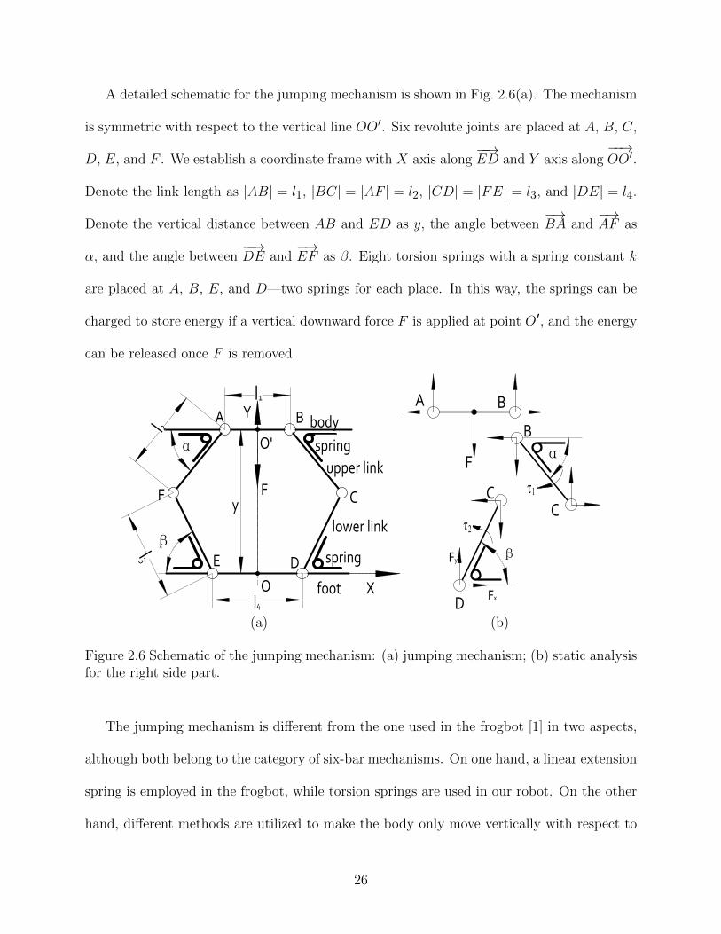
A detailed schematic for the jumping mechanism is shown in Fig. 2.6(a). The mechanism

is symmetric with respect to the vertical line OO′. Six revolute joints are placed at A, B, C,

D, E, and F . We establish a coordinate frame with X axis along−−→ED and Y axis along

−−→OO′.

Denote the link length as |AB| = l1, |BC| = |AF | = l2, |CD| = |FE| = l3, and |DE| = l4.

Denote the vertical distance between AB and ED as y, the angle between−→BA and

−→AF as

α, and the angle between−−→DE and

−→EF as β. Eight torsion springs with a spring constant k

are placed at A, B, E, and D—two springs for each place. In this way, the springs can be

charged to store energy if a vertical downward force F is applied at point O′, and the energy

can be released once F is removed.

B

X

F

O'

Y

O

A

y

body

l1

F C

lower link

spring

α

βl3

springupper link

l2

l4

DE

foot

(a)

A

F

B

C

D

βFy

Fx

τ2

Bα

τ1C

(b)

Figure 2.6 Schematic of the jumping mechanism: (a) jumping mechanism; (b) static analysisfor the right side part.

The jumping mechanism is different from the one used in the frogbot [1] in two aspects,

although both belong to the category of six-bar mechanisms. On one hand, a linear extension

spring is employed in the frogbot, while torsion springs are used in our robot. On the other

hand, different methods are utilized to make the body only move vertically with respect to

26

the foot. The frogbot employs two pairs of gears at both the body and the foot, while our

robot relies on the symmetric placement of torsion springs.

For the mechanism optimization in section 2.4, we analyze the statics for the required

force F—which varies with distance y—to charge the energy. Since the mechanism is sym-

metric with respect to OO′, analysis for the right side part is sufficient. Fig. 2.6(b) shows

the free body diagrams for links AB, BC, and CD, where all forces are decomposed along

the coordinate frame axes. The component forces along the same axis, except F , have the

same quantity, although the directions may be opposite. Denote the same quantity as Fx

and Fy along the x axis and y axis, respectively. From the figure, the static equations for

the three links are:

F = 2Fy

τ1 = 2k(π

2− α) = Fxl2 sinα + Fyl2 cosα

τ2 = 2k(π

2− β) = −Fxl3 sin β + Fyl3 cos β

where τ1 and τ2 are the torques generated by the springs. From the above equations, F can

be solved as:

F =2kl3(π − 2α) sin β + 2kl2(π − 2β) sinα

l2l3 sin(α + β)(2.11)

Note that α and β are functions of y and point C’s vertical coordinates yC . Point C is the

intersection point of two circles with centers at B : (l1/2, y) and D : (l4/2, 0); therefore, yC

can be solved as:

yC =y

2−y(l22 − l

23)

2e+ld4e

√[(l2 + l3)2 − e][e− (l2 − l3)2] (2.12)

27

where e = l2d/4 + y2 with ld = l4 − l1. In fact, there are two intersection points for those

two circles, but the point corresponding to the configuration shown in Fig. 2.6(a) is unique.

Once yC is obtained, we can solve α and β as:

α = arcsiny − yCl2

, β = arcsinyCl3

(2.13)

Substituting Eqs. (2.12) and (2.13) into (2.11), we can express F as a function of y by

eliminating α, β, and yC .

To facilitate the optimization in section 2.4, let ymax and ymin be the maximum and

minimum value of y. The largest value for ymax is√

(l2 + l3)2 − l2d/4 when AF and FE,

BC and CD are collinear. However, we cannot achieve this value because it corresponds to

the singular configuration which we should stay clear. Meanwhile, ymax should be as large

as possible so that the energy stored in the spring can be released thoroughly. To simplify

the design process, we empirically let:

ymax = 0.95√

(l2 + l3)2 − l2d/4 (2.14)

2.3.2 Energy Mechanism

For the jumping mechanism, another energy mechanism is required to store energy and

release it when necessary. Generally, this can be achieved in two ways. The first approach

rotates the motor in one direction to charge energy and in the other direction to release

energy. Examples include the scout robot [15] and our second robot [14]. The second

approach rotates the motor in a single direction for energy charge and release, leading to a

short cycle time. This can be achieved by a slip-gear system [2, 5], an eccentric cam [49, 9],

28

F

body

rotation link

foot

cablepulley

(a) (b) (c)

Figure 2.7 Illustration of the energy mechanism: (a) intermediate position during the chargeof energy; (b) critical position; (c) intermediate position during the release of energy.

or a variable length crank mechanism [18]. To obtain a short cycle time, we propose a new

energy mechanism belonging to the second approach. The key element in this mechanism is

a one way bearing.

Fig. 2.7 illustrates the energy mechanism. A rotation link is connected to the output

shaft of a speed reduction system via a one way bearing not shown in the figure. Due to the

one way bearing, the rotation link can only rotate in the counterclockwise direction. A cable,

guided by two pulleys, connects the end of rotation link to the robot’s foot. If the rotation link

rotates from the bottom vertical initial position, the cable forces the body to move towards

the foot (Fig. 2.7(a)). The rotation link’s top vertical position (Fig. 2.7(b)) is a critical

position since the torque resulted from the cable will switch its direction. Once the link

passes this position, the energy is released, and the body accelerates upward (Fig. 2.7(c)).

The body and foot in Fig. 2.7 are the same parts in the jumping mechanism shown in

Fig. 2.6(a), but the links are not shown for a clear view.

29

φ

F

O T

lbl a

pulleyFigure 2.8 Statics for the energy mechanism.

With such a mechanism, the force F in Fig. 2.6(a) can be applied for energy charge. For

the optimization in section 2.4, we perform the static analysis for the rotation link to relate

this force to the torque generated by the speed reduction system. As shown in Fig. 2.8, la

is the length of the rotation link, and lb is the vertical distance from the end of the rotation

link to the pulley’s center. If the link is rotated to a new position shown as the dashed line

in the figure with a rotation angle φ ∈ [0, π], then the required torque T is equal to the

torque generated by F with respect to pivot point O:

T =Fla(la + lb) sinφ√

l2a + (la + lb)2 − 2la(la + lb) cosφ

(2.15)

For the optimization in section 2.4, we also represent the vertical distance y between the

body and the foot shown in Fig. 2.6(a) as:

y = ymax − (√l2a + (la + lb)

2 − 2la(la + lb) cosφ− lb) (2.16)

30

2.3.3 Self-righting Mechanism

With the jumping and energy mechanisms, the robot can jump if it initially stands on

the ground with its foot. This case, however, seldom happens due to the landing impact.

Therefore, a self-righting mechanism is needed to make the robot recover from possible

landing postures.

In general, there are two methods for self-righting. The first one is the passive recovery

based on the center of gravity (CoG). The robot will stand up if the CoG is sufficiently

close to the foot. Examples include the EPFL jumper V3 [11], the Jollbot [18], and our

first robot [13]. The second method, widely used in animals, is the active recovery with

actuated parts. For instance, the beetles employ their legs for self-righting [93], while the

turtles utilize the head because of their short legs [94]. The active recovery is implemented

in the frogbot [1] and the new surveillance robot [3]. For our robot, we adopt the active

self-righting to achieve a small robot size.

Fig. 2.9 illustrates the working principle for our self-righting mechanism. The robot has

a rectangular shape with two surfaces significantly larger than the other four. As a result,

the robot will contact the ground with one of these two large surfaces most of the time after

landing. Without loss of generality, we assume a landing posture as shown in Fig. 2.9(a).

Two self-righting legs on the body are initially parallel to the two large surfaces. Once

actuated, they can rotate simultaneously in opposite directions. After a certain amount of

rotation, the robot can stand up for the next jump. The final position when both legs are

fully extended is shown in Fig 2.9(b).

The detailed mechanism is shown in Fig. 2.10, where the whole mechanism is shown on

the left and a partial enlargement is shown on the right. Note that the foot is not shown for

31

footleft leg

right legbody

(a)

left leg right leg

(b)

Figure 2.9 Illustration of the self-righting mechanism: (a) initial position after the robotlands on the ground; (b) final position when the robot stands up.

B

C

A

spring

body

right legleft leg upward force

pin

Figure 2.10 Details of the self-righting mechanism.

a clear view. A revolute joint connects each leg to the body. A pin (shown as a solid circle

in the enlargement) fixed to the left leg can slide along a groove in the right leg. In this way,

if we apply an upward force on the pin, both legs will rotate, but in opposite directions. A

small torsion spring—with one end fixed to the body and the other end attached to the left

leg—will make both legs return to their original positions if the upward force is removed.

We apply the upward force in Fig. 2.10 using the same actuator for energy charge. In

fact, the body moves towards the foot during the energy charge process. With this motion, if

a protrusion is attached to the foot and beneath the pin, the upward force will be generated

once the protrusion contacts the pin. If the energy is released, the body will move away from

32

the foot; consequently, the upward force is removed when the body is a certain distance away

from the foot.

From the above discussions, the energy charge and the self-righting can be performed

simultaneously, leading to a short cycle time. Furthermore, all the motion can be accom-

plished with the motor’s one directional rotation. Note that the frogbot also employs a

single motor for the energy charge and the self-righting. The self-righting process, however,

is divided to two phases due to the shape of the robot [1].

2.3.4 Steering Mechanism

The final mechanism to realize the motion sequence in Fig. 2.2 is the steering mechanism,

which can change the jumping direction. A review of steering methods for jumping robot

can be found in [11]. Based on our robot’s rectangular shape, we propose a steering method

without extra actuators.

The steering mechanism is illustrated in Fig. 2.11. Two steering gears are placed sym-

metrically about the motor gear. Both gears are a certain distance away from the robot’s

centerline. Since the robot contacts the ground with one of its two large surfaces after land-

ing, one of the two steering gears will touch the ground. Therefore, if the motor rotates, the

robot will change its heading direction.

The same motor for the other three mechanisms actuates the steering mechanism. In

fact, the steering mechanism is driven by the motor’s one directional rotation, while the

other three mechanisms are actuated by the other directional rotation. One steering gear

is also used in the speed reduction system for energy charge. If the motor rotates in one

direction, this gear is used for energy charge. If the motor rotates in the other direction, the

rotation link in Fig. 2.7 will not rotate due to the one-way bearing. In this case, this gear

33

center line

foot foot

(a)

steering gear

foot steering gear

motor gear

(b)

Figure 2.11 Illustration of the steering mechanism: (a) front view; (b) side view.

can steer the robot.

The steering mechanism is improved from our previous design in [88], where a single large

gear at the end of speed reduction system is the steering gear. Due to its large diameter,

the gear can touch the ground no matter which large surface of the robot contacts the

ground. This method, although simpler, has a slow steering speed due to the large gear’s

small angular velocity. The new design increases the speed because the two steering gears

are next to the motor gear, resulting in a large angular velocity.

2.4 Design Optimization

Based on the analysis in section 2.3, the mechanism dimensions can be determined through

optimization. In this section, we optimize the jumping mechanism together with the energy

mechanism to obtain the smallest peak torque for energy charge. After that, the dimensions

of the self-righting mechanism are derived based on practical requirements. The steering

mechanism is not discussed because it is determined by the energy mechanism.

34

Table 2.1 List of parameters for optimization

l2 length of the upper link (Fig. 2.6(a))l3 length of the lower link (Fig. 2.6(a))ld difference between the body link l1 and the foot link l4la length of the rotation link (Fig. 2.8)lb vertical distance from the rotation link to the pulley (Fig. 2.8)y vertical distance between the body and the foot (Fig. 2.6(a))α angle between the body link and the upper link (Fig. 2.6(a))β angle between the foot link and the lower link (Fig. 2.6(a))φ angle between the rotation link and the vertical line (Fig. 2.8)E0 total energy stored in the springk torsion spring constant

2.4.1 Jumping Mechanism and Energy Mechanism

With the jumping and energy mechanisms, if the same energy can be charged with a small

peak value of torque T generated by the speed reduction system, then the weight and size

for the robot can be reduced. Therefore, optimization is needed to minimize the peak value

of T .

In the following, we perform the optimal design in four steps: identifying the optimization

variables, formulating the objective function, obtaining the constraints, and solving the con-

strained optimization problem. For easy reference, the parameters used in the optimization

are listed in Table 2.1.

To identify the optimization variables, we substitute the force equation (2.11) into the

torque equation (2.15):

T =2kla(la + lb) sinφ[l3(π − 2α) sin β + l2(π − 2β) sinα]

l2l3 sin(α + β)√l2a + (la + lb)

2 − 2la(la + lb) cosφ(2.17)

from which there are eight parameters: k, la, lb, α, β, l2, l3, and φ. Since α and β can be

written as a function of y, l2, l3, and ld by substituting Eq. (2.12) into Eq. (2.13), the true

35

parameters are k, la, lb, y, l2, l3, ld, and φ.

Among the eight parameters, the variables will be only lb, l2, l3, ld, and φ because k, la,

and y are either constants or dependents on the variables. First, according to our previous

design [88], the torsion springs are chosen to have a constant k = 58.98Nmm/rad. Second,

la can be obtained from l2, l3, and ld. In fact, from the geometrical relation of the energy

mechanism, we have la = (ymax − ymin)/2. If l2, l3, and ld are given, ymax can be derived

using Eq. (2.14). With ymax known, ymin can also be determined to ensure a desired initial

energy E0 can be stored in the springs. Third, once ymax and la are known, y can also

be derived through Eq. (2.16) based on lb and φ. From the above arguments, T is only a

function of lb, l2, l3, ld, and φ, and we denote it as T (lb, l2, l3, ld, φ). The optimization

variables are only lb, l2, l3, and ld because φ will run from 0 to π during each energy charge

cycle.

The initial energy E0 is determined based on the simulations in section 2.2. To achieve

one meter jumping height with a 75 take-off angle, the initial energy should be 0.3J. But

to leave enough margin, we let E0 = 0.4J. In addition, the zero energy configuration for the

jumping mechanism corresponds to the configuration when y = ymax. The α and β angles

for such a configuration depend on the link lengths and can be derived using Eqs. (2.12) and

(2.13).

Having identified the optimization variables, we formulate the objective function. Given

lb, l2, l3, and ld, a torque curve as φ running from 0 to π can be plotted. The goal is to find

the optimal lb, l2, l3, and ld such that the peak torque in the curve is the minimum among

all possible curves. Therefore, the objective function is the peak torque in the curve:

g(lb, l2, l3, ld) = maxφ∈[0, π]

T (lb, l2, l3, ld, φ) (2.18)

36

The next step is to obtain the constraints for the optimization variables. The lengths

of l2 and l3 should be large enough to hold the torsion springs. But they cannot be too

large due to the size limit of the robot. Therefore, with practical considerations, assume

15mm ≤ l2, l3 ≤ 20mm. With similar implementation reasons, we can have other linear

constraints for lb and ld, and the optimization can be formulated as:

minimize g(lb, ld, l2, l3)

subject to 7 ≤ lb ≤ 12, −5 ≤ ld ≤ 5,

15 ≤ l2 ≤ 20, 15 ≤ l3 ≤ 20 (2.19)

where the omitted length unit is millimeter.

To solve the constrained optimization problem, we apply the numerical method because

the analytical expression for g(lb, ld, l2, l3) cannot be obtained. The optimization is realized

by a dense discretization of φ and value evaluations at the resulting points [95]. The con-

strained nonlinear multivariable function in the Optimization Toolbox of Matlab is employed

to find the optimal value. Since the method can only obtain the local minimum, we choose

various random initial points to run the optimization. The smallest objective function a-

mong these local minima is the optimal value, and the optimal dimensions are lb = 7mm,

ld = 1.2mm, l2 = 15mm, and l3 = 20mm. The other parameters can be calculated accord-

ingly: ymax = 33.3mm, ymin = 11.7mm, and la = 10.8mm. To avoid interference between

the two revolute joints at the foot, let l1 = 18mm, then l4 = l1 + ld = 19.2mm.

To investigate how the variables affect the objective function, we plot the graphs showing

the objective function and the variables. Since it is impossible to include the four variables

into one graph, we divide them into two groups: lb and ld, l2 and l3. Fig. 2.12(a) shows how

37

−5

0

5

68

1012

175

180

185

190

195

ld (mm)l

b (mm)

T (

Nm

m)

(a)

1416

1820

1416

1820

175

180

185

190

195

l2 (mm)l

3 (mm)

T (

Nm

m)

(b)

Figure 2.12 Objective function varies with optimization variables: (a) variation ofg(lb, ld, l2, l3) with fixed l2 and l3; (b) variation of g(lb, ld, l2, l3) with fixed lb and ld.

the objective function changes with respect to lb and ld by fixing l2 and l3 to the optimal

value. As seen in the figure, the minimum value happens when lb is the smallest and ld is in

the middle part. Fig. 2.12(b) shows how the objective function varies with respect to l2 and

l3 by fixing lb and ld to the optimal value. In this figure, the minimum value happens at the

left corner. From these two figures, we see that the optimal dimensions obtained from the

optimization are correct.

0 50 100 150 2000

50

100

150

200

φ (degree)

T (

Nm

m)

Figure 2.13 Torque profile with the optimal dimensions.

38

With the optimal design, we can obtain the torque curve with respect to the angle φ

as shown in Fig. 2.13. From the figure, the torque profile is nonlinear with the peak value

happening at φ = 66. Furthermore, the torque is zero when the energy is about to be

released (φ = 180), which means the release of the energy requires the minimal torque.

With the small torque during the release, the mechanism can reduce the probability of

premature take-off [1]; consequently, it is highly possible that all the energy stored in the

spring can be converted to the kinetic energy for take-off.

2.4.2 Self-righting Mechanism

The dimensions for the self-righting mechanism are critical for successful recovery from possi-

ble landing postures. The design variables include the leg length and the range of leg rotation

angle. The initial and final positions for both recovery legs are shown in Fig. 2.14(a). The

initial positions, AM and BN , are parallel to the body, and the final positions, AM ′ and

BN ′, contact the ground with leg ends M ′ and N ′. The ranges of leg rotation angle are

denoted by µ and ν for the left and right leg, respectively. O is the middle point for AB.

Moreover, we have AB ⊥ OD and ∠ODN ′ = θ = 75, which is the robot take-off angle.

The relation between the leg length and the range of leg rotation angle can be obtained using

the law of sines in 4AM ′E and 4BN ′F :

|AM ′|sin(π − θ)

=|OD|+ |AO| tan(π/2− θ)

sin(µ− π + θ)(2.20)

|BN ′|sin θ

=|OD| − |BO| tan(π/2− θ)

sin(ν − θ)(2.21)

39

footE D F

B

A

left leg

right legbody

Oμ

ν

MN

M' N'

C'

C

(a)

C1

BA

C2

C4

C5

OC3

(b)

Figure 2.14 Dimension design of the self-righting mechanism: (a) mechanism with initial andfinal positions for both self-righting legs; (b) simplification of the mechanism to determinethe length for link AC.

From Eqs. (2.20) and (2.21), if µ or ν is large, then the leg length AM ′ or BN ′ can be small.

To simplify the design, we fix µ = 135 and ν = 105 to let µ−∠ODM ′ = ν−∠ODN ′ = 30.

With µ and ν fixed, |AM ′| and |BN ′| can be solved from Eqs. (2.20) and (2.21) given

|AO| = |BO| and |OD|, which are determined from the implementation.

The next step is to design the length of AC shown in Fig. 2.14(a) to achieve the desired

angle ranges. Without the body, the foot, the part AM in the left leg, and the part BN

in the right leg, the mechanism can be simplified as shown in Fig. 2.14(b). In the figure,

C1 to C5 are different locations for the end point C of link AC. C1 and C5, symmetric

with respect to AB, are the limit position for link AC; therefore, ∠C1AC5 = µ = 135.

C2 and C4, symmetric with respect to AB as well, are the tangent points from point B

to the circle formed by link AC. Since BC2 and BC4 are the limit positions for link BC,

∠C2BC4 = ν = 105. From right-angled 4ABC4, we have |AC| = |AB| sin(ν/2). The

parameters for the right leg can also be derived accordingly.

40

lower Link

upper Link springs

foot

body

(a)

motor

body

cable

pulley

rotation link

gear train

(b)

pusher

left leg

right leg

pin

spring

body

(c)

steering gear

steering gearmotor gear

(d)

Figure 2.15 Solid model for each mechanism (a) jumping mechanism (principle shown inFig. 2.6(a)); (b) energy mechanism (principle shown in Fig. 2.7); (c) self-righting mechanism(principle shown in Fig. 2.10); (d) steering mechanism (principle shown in Fig. 2.11).

2.5 Fabrication and Experimental Results

2.5.1 Fabrication and Development

The solid model for the robot is shown in Fig. 2.1(b), and the individual mechanisms are

shown from Fig. 2.15(a) to Fig. 2.15(d). Some parts appear in multiple figures because they

are used in different mechanisms. We elaborate the implementation for each mechanism in

this sub section.

For the jumping mechanism shown in Fig. 2.15(a), both the left-hand (9287K77 from

McMaster-Carr) and the right-hand (9287K26 from McMaster-Carr) torsion springs are re-

quired. We use a pin-hole structure to implement the revolute joints. The torsion springs

are held in place by the pins of the revolute joints. The bottom of the foot is designed with

a tilted angle 15 to provide the 75 take-off angle.

The major part of the energy mechanism, shown in Fig. 2.15(b), is the motor actuated

gear train or speed reduction system. The gear train has three stages consisting of a motor

gear (8 teeth), a compound gear (28/8 teeth), another compound gear (28/9 teeth), and

a spur gear (35 teeth). Therefore, the total speed reduction ratio is 47.6. Based on this

41

ratio and the required peak torque (178Nmm) in Fig. 2.13, the motor (GH810136V3 from

Gizmoszone) with a stall torque 8Nmm is chosen. For this motor, a sufficient margin has

been left to overcome the friction in the gear train. The one-way bearing (kit8637 from VXB

bearings) cannot be shown in Fig. 2.15(b) because it is inside the rotation link.

Fig. 2.15(c) shows a section view of the self-righting mechanism. The revolute joints

connecting the two legs to the body are achieved by the pin-hole structure as well. The

pusher attached to the foot—not shown in Fig. 2.15(c)—can provide the upward force in

Fig. 2.10. The small torsion spring (9287K12 from McMaster-Carr) is held in placed by the

pin in the left revolute joint.

The steering mechanism, shown in Fig. 2.15(d), comes from the energy mechanism. All

of the gears in the gear train of Fig. 2.15(b) are shown in Fig. 2.15(d). Only the right steering

gear does not belong to the energy mechanism, and the left steering gear is part of the gear

train to charge energy.

We obtain the robot parts from three sources. First, some parts are off-the-shelf compo-

nents such as springs and bearings. Second, most of the other parts are fabricated using the

selective laser sintering with the DuraForm HST material. It has a density only 1.20g/cm3,

yet it can be used for functional prototypes. Third, the aluminum shafts in the gear train

are manufactured using traditional machining methods.

The robot is powered by a FullRiver 50mAh LiPo battery with an average 3.7V voltage

output. Since the energy mechanism is placed on the right side of the body, the battery—

shown in Fig. 2.1(b)—is placed on the left side to balance the robot’s weight.

Depending on the obstacle size the robot needs to overcome, we can adjust the robot’s

parameters in two ways to achieve different jumping performances. First, the take-off angle

can be modified by using feet with different tilted angles. In this way, the ratio between the

42

jumping height and distance varies according to Eqs. (2.3) and (2.4). Second, the torsion

springs in the jumping mechanism can be replaced by those with smaller constants. In this

case, the initial stored energy in the robot can be changed, leading to different jumping

performances.

For the robot, the mass and the initial stored energy are needed to obtain the theoretical

performances. The lower part of the robot contains the components below the revolute joint

connecting the lower link to the upper link, while the upper part includes all of the other

components above that joint. The mass for each part is m1 = 5.4g and m2 = 18.1g. The

initial energy E0 is designed to be 0.4J, but the true energy cannot be this much because

the minimum distance ymin for y cannot be the designed value due to the cable’s elasticity.

Therefore, the true ymin is measured to calculate the energy stored in the spring. In fact,

ymin = 14mm and the resulting E0 = 0.34J.

2.5.2 Experimental Results

Jumping experiments are conducted to determine the jumping performances. To eliminate

the slippage during the robot’s take-off, we place the robot on a high coefficient of friction

surface (fine grained sand paper with a grit designation 320). To obtain the performances, we

also place the robot in front of a board with small holes. The distance between neighboring

holes, either horizontal or vertical, is one inch (2.54cm). When the robot jumps, a video is

recorded by a Casio Exilim EX-FH25 high speed camera with a frame rate 240 frame-per-

second. After that, the jumping height is obtained off-line from the video by comparing the

robot’s highest position with the vertical holes, while the jumping distance is obtained by

comparing the landing position with the horizontal holes.

Five jumps are carried out to obtain the average jumping performance. The average

43

jumping trajectory for these five jumps is plotted with the solid line in Fig. 2.16. Note that

the robot jumps from the right to the left, and only half of the trajectory is shown due to the

symmetry of the trajectory. The average performance is listed in Table 2.2, where the robot

can jump 87.2cm in height and 89.8cm in distance. The standard deviations for these jumps

are 2.2cm and 4.0cm for the height and distance, respectively. The take-off velocity can also

be obtained as 4.3m/s. Therefore, the jumping efficiency—defined as the ratio between the

kinetic energy before robot’s take-off E and the initial stored energy E0—is 63.0%.

0204060800

10

20

30

40

50

60

70

80

90

Horizontal Distance (cm)

Ver

tical

Dis

tanc

e (c

m)

Without extra weightWith 4g extra weightWith 8g extra weight

Figure 2.16 Jumping experimental results: average trajectories for three sets of experiments.

The sensor network application requires the robot to be able to carry payloads for extra

sensors. Therefore, experiments are conducted to investigate the jumping performance with

an extra weight. The extra weight is placed on the opposite side of gear train to balance

the robot’s weight. The average performances for five jumps are listed in Table 2.2 as well,

and the average trajectories are also shown in Fig. 2.16. For an extra four gram mass, the

average jumping height and distance are 82.1cm and 80.6cm, respectively. If an extra eight

gram mass is added, the average jumping height and distance become 69.5cm and 67.8cm,

44

Table 2.2 Experimental and Theoretical Jumping Performances

ExtraWeight

ExperimentalHeight (cm)

ExperimentalDistance (cm)

EstimatedHeight (cm)

EstimatedDistance (cm)

0g 87.2± 2.2 89.8± 4.0 97.9 103.44g 82.1± 1.2 80.6± 1.6 88.9 94.28g 69.5± 2.2 67.8± 2.8 81.1 86.1

respectively. The small decreases in both the jumping height and distance are not large

indicates the robot can carry some payloads without degrading its performance significantly.

The theoretical performances with the air resistance are also listed in Table 2.2. From

the table, the experimental results are worse than the theoretical calculations. The major

reason for such a discrepancy is the friction in the jumping mechanism. In particular, the

friction exists in all of the revolute joints since they are built using the pin-hole structure.

Due to the friction, only part of the stored energy is converted to the kinetic energy for

take-off. Additionally, some energy is also transformed to the robot’s rotation energy in the

air. This energy loss, however, is negligible because of the robot’s small moment of inertia

and angular velocity.

t=0s t=1s t=2s t=3s t=4s t=5s

Figure 2.17 Self-righting experimental result: six individual frames extracted from a self-righting video.

45

46

Table 2.3 Comparison with existing robots with the jumping ability

Robot Name Mass[g]

Size[cm]

Chargetime[s]

Jumpheight[cm]

Jumpdistance[cm]

Normalizedjumpheight [cm]

Height permass and size[10·cm·/(g·cm)]

Self-right

Steer Onboardenergy

Actuator

Flea robot [20] 1.1 2 15 64 70 68.8 312.73 no no no 3 SMAFrogbot [1] 1300 15 30 90 200 117.8 0.06 yes yes yes 1 motorSurveillance robot[3]

150 12.2 60 105 60 107.1 0.59 yes no yes 2 motors

Grillo III [7] 22 5 8 10 20 12.5 1.14 no no yes 1 motorEPFL jumper V1[9]

6.98 5 3.5 138 79 140.8 40.34 no no yes 1 motor

EPFL jumper V2[10]

9.8 12 3.5 76 81 81.4 6.92 yes no yes 1 motor

EPFL jumper V3[11]

14.33 18 3.5 62 46 64.1 2.49 yes yes yes 2 motors

Multimodal robot[12]

72 × × 170 0 170 × no no yes ×

Compact jumpingrobot [16]

18 11 0.3 15 95 52.6 2.66 no no no 2 motors

MIT microbot [17] 46 10 × 38 0 38 0.83 no no no 1 DEAJollbot [18] 465 30 1.44 18.4 0 18.4 0.01 yes yes yes 2 motorsDeformable robot[19]

5 9 45 18 0 18 4 yes no no 4 SMA

MSU jumper 23.5 6.5 10 87.2 89.8 93.0 6.09 yes yes yes 1 motor

× Data are not available from the reference

46

The self-righting experiments are also carried out. One of the results is shown in Fig. 2.17,

where six frames from a video recording the self-righting process are presented. The robot

needs five seconds for self-righting as seen from the time under each picture. Since the self-

righting process is performed simultaneously with the energy charge process, the cycle time

does not increase.

The steering experiments are performed on the ground as well. Four frames from a

video are shown in Fig. 2.18. In this experiment, the robot changes its direction in the

counterclockwise direction. From the video, the robot can rotate 360 in about 10 seconds;

therefore, the rotation speed is about 36/s, which is much faster than the 2/s for our

previous design [88].

t=0s t=1s t=2s t=3s

Figure 2.18 Steering experimental result: four individual frames extracted from a steeringvideo.

2.5.3 Comparison with Other Robots

Comparisons with other jumping robots are listed in Table 2.3. Since robots with different

energy storage methods have different characteristics, only the robots based on traditional

and customized springs are listed. Furthermore, some robots are not included because they

use wheels as the primary locomotion method such as the mini-whegs [5], the stair climbing

robot [8], and the scout robot [15].

47

To make the comparison fair, appropriate indices should be chosen. The mass, size,

jumping height, and jumping distance are usually selected for comparison [18]. In Table 2.3,

these four indices are listed in column two, three, five, and six, respectively. Note that the

size is the maximum dimension among the length, width, and height. For spring based

robots, the charge time—fourth column in the table—is also an important index since more

energy can be stored with a longer charge time provided the other conditions are the same.

Since the jumping height and distance vary with take-off angles, the normalized jumping

height with a 90 take-off angle is calculated from the jumping height and distance using

Eqs. (2.3) and (2.4). This index is the seventh column in the table. To compare the obstacle

height the robot can overcome given its size and weight [47], the height per mass and size

is listed in the eighth column. It is obtained from dividing the normalized jumping height

by the mass and the size. The subsequent three columns indicate whether the robot has

self-righting, steering, and onboard energy, respectively. Finally, the type and the number

of actuators are listed in the last column.

Compared with the robots in Table 2.3, the MSU jumper has a good overall performance

among those robots with continuous steerable jumping ability. The overall performance is

indicated by the height per mass and size index (the eighth column in Table 2.3). Besides the

good overall jumping performance, the MSU jumper employs a single motor for continuous

steerable jumping. Except the frogbot and those robots with different actuation methods,

all of the other robots need extra motor to achieve either self-righting or steering as indicated

in the last column of Table 2.3.

Compared with the MSU jumper, the other jumping robots have their own merits as

well. First, the robots with wheels can run faster if no obstacle exists [5, 15]. Second, the

robots with a sphere structure for self-righting can roll passively on the ground. Moreover,

48

the enclosed sphere protects the robot from damage [10, 11, 18]. Third, some robots have

the embedded sensing, control, and communication system [1, 3]. With such a system, the

control, navigation, and motion planning can be investigated for the jumping locomotion [96].

2.6 Conclusions

To facilitate the locomotion for mobile sensors in environments with obstacles, this chapter

presents the mechanical design of a miniature steerable jumping robot. Different from exist-

ing designs, the robot can satisfy three design requirements: continuous steerable jumping,

minimum actuation, and light weight. Moreover, optimal design is performed to obtain the

best mechanism dimensions. Experimental results show that the robot has a good overall

jumping performance compared with existing jumping robots. The jumping robot in this

chapter can be potentially used in mobile sensor networks for various applications. Further-

more, the design method presented in this chapter may also be applied to other miniature

robot designs.

49

Chapter 3

MSU Tailbot: A Biologically Inspired

Tailed Robot

3.1 Introduction

Many animals use multiple locomotion methods to travel in natural environments under

different situations [31]. For example, a lizard can rapidly jump up to seize small insects or

escape from predators; it can also walk slowly in other non-emergent situations. Further,

once leaping into the air, it can use the tail to control its body angle for safe landing [60].

The various locomotion abilities found in animals inspire many novel robot designs with

multi-modal locomotion [97].

Robots with multi-modal locomotion abilities are required as the deployment of robots

in natural environments becoming more widespread. Consider the scenario of using many

miniature robots to monitor an environment with obstacles. The energy efficient way is to

employ wheeled locomotion if there is no obstacle. Encountering a large obstacle, the robot

can jump to cross it. Moreover, to protect the robot from damage during the landing, it is

desirable that the robot can perform aerial maneuvering to control its body angle to land

on the ground with a safe posture.

In this chapter, we present the design, control, and experimentation of a robot that can

accomplish the above multi-modal locomotion. The detailed motion cycle for the robot is

50

Self‐right & charge energy

Release energy & jump into air

Control orientation in mid‐air

Land on the ground

Wheel on the ground

No obstacle

Encountering an obstacle

Figure 3.1 The robot motion cycle with the robot prototype in the center.

shown in Fig. 3.1 with the robot prototype in the center of the figure. The robot can jump

up to 80 cm with a mass of 26.5 grams and a maximum body size 7.5 cm. Moreover, the

robot has onboard energy, sensing and control, and wireless communication abilities, which

make it an ideal mobile sensor platform for wireless sensor networks. To the best of our

knowledge, this is the first miniature, lightweight, and tetherless robot that has all of the

wheeling, jumping, and aerial maneuvering abilities.

Two main challenges exist for developing such a robotic platform. First, it is difficult to

perform real time onboard control for aerial maneuvering since the jumping time only lasts

for less than one second and the robot needs to perform real time sensing, computation, and

control. Second, it is challenging to design a robot with a small size and a light weight yet

having all the jumping, wheeling, and aerial maneuvering capabilities.

The major contributions of the robot presented in this chapter can be summarized into

51

two aspects. First, based on our previous robot with a tail [98], we present the design and

development of a miniature robot that has three locomotion capabilities: wheeling, jumping,

and aerial maneuvering. Although there exists robots having two of them, none has all of

the three. Second, we present the detailed dynamic analysis and controller design for the

aerial maneuvering using an active tail. Although the dynamics model has been obtained

before [60, 62], only the PD controller is adopted for the stabilization control. In this

chapter, however, we transform the dynamics model into the standard nonlinear form and

design advanced controllers such as nonlinear feedback controller and sliding mode controller.

The remainder of this chapter is organized as follows. First, the detailed robot design is

presented in section 3.2. Then, we elaborate the dynamics modeling for aerial maneuvering

and optimize the design of the tail to obtain the best dynamic performance in section 3.3.

Based on the dynamics model, controllers are designed including a sliding mode controller

and a PD controller in section 3.4. Finally, we present simulation and experimental results

for aerial maneuvering and demonstrate the multi-modal locomotion abilities of the tailbot.

3.2 Robot Design

The robot design, including mechanical and electrical design, will be elaborated in this

section.

3.2.1 Mechanical Design

The solid model and the working principle of the tailbot are illustrated in Fig. 3.2. The

whole robot can be divided into two parts: the tail part and the body part as shown in

Fig. 3.2(a).

52

For the tail part, we implement a tail with one degree of freedom to control the body’s

pitch angle. Fig. 3.2(c) illustrates the detailed design of the tail part. The tail and the body

are connected by a revolute joint actuated by a DC motor—labeled as tail motor in the

figure. A motor gear is directly attached to the shaft of the motor, and a tail gear meshes

with the motor gear. A carbon fiber rod with a steel block shown in Fig. 3.2(a) is fixed to

the tail gear. Note that only part of the rod is shown in Fig. 3.2(c). Two teeth of the tail

gear are removed to avoid the interference between the tail and the body at limit positions.

This is also useful for the wheeling part that will be discussed later.

The tail can also be utilized for mode transition: from wheeling mode to jumping mode

and vice versa. On one hand, when the robot wheels on the ground, the tail can push the

ground to have the robot stand up and be ready for the next jump. On the other hand, when

the robot stands for jumping, the tail can also push the ground to make the robot lie down

for wheeling. The detail process can be found in the experimental part for mode transition.

The design for the tail part should ensure rapid control of the body’s orientation since

the jumping process lasts for a short time (less than one second for a one meter jumping

height). Therefore, an optimal design will be performed to obtain the optimal parameters

for the tail based on the dynamics model in the next section.

The body part comes from the MSU jumper. It consists of two major components:

the jumping mechanism and the energy mechanism. Since the detailed design is already

discussed in the previous chapter, we omit them here. However, the working principles for

these two mechanisms are illustrated in Fig. 3.2(e) and (f), respectively.

The foot has a tilted angle of 15 to make it take off at an angle of 75. However, since

the revolute joints in the jumping mechanism are realized by a pin-hole structure, the takeoff

angle may vary within ±5 as demonstrated in our previous experiments [99].

53

(a) (b)

(c)

(d)

(e)

(f)

rigid link

cable

platform

foot

cable

upper link

lower link

springs

platform

foot

jump motor left wheeling gear

rod

tail gear

right wheeling gear

spring

tail motor

7.5cm

tail

body

5.2 cm

block

rod

rigid link

7.4 cm

upper link

lower link

platform

jump motor tail motor

foot

springs

Figure 3.2 Mechanical design of the tailbot: (a) Left view with height and width, and therobot is divided into the body and tail part encircled by two rectangles; (b) Front viewwith length, and two major parts encircled by two rectangles are shown in (c) and (d),respectively; (c) Section view of the tail part; (d) Section view of the gear train part for theenergy mechanism; (e) Working principle of the jumping mechanism; (f) Working principleof the energy mechanism.

In addition to the jumping mechanism and energy mechanism, the robot has two wheeling

gears as shown in Fig. 3.2(c) and (d), which are employed for differential drive on the ground.

Note that the robot’s wheeling posture, once it lands on the ground, can be guaranteed. In

fact, the robot has a rectangular shape with two sides much larger than the other four;

therefore, it will land on the ground with one of the two large sides. It can wheel if it lands

with the side having the two wheeling gears on the ground. If it lands with the other large

side, the tail can rotate to turn the robot upside down so that the robot can still wheel on

the ground.

The wheeling part does not require extra actuation. The left wheeling gear is part of the

gear train for the energy mechanism as shown in Fig. 3.2(d). If the jump motor rotates in

one direction, the rigid link will rotate to charge and release the energy. But if the motor

rotates in the opposite direction, the rigid link will stay still due to the one-way bearing. In

this case, the left wheeling gear is used for the wheeling motion.

54

The right wheeling gear is actuated by the tail motor as shown in Fig. 3.2(c). Since

the tail gear has two teeth removed, once the tail reaches the left limit position shown in

Fig. 3.2(c), the counterclockwise rotation of the motor gear cannot actuate the tail. In this

case, the right wheeling gear can be used for the wheeling motion. To switch from wheeling

mode to jumping mode, a small extension spring placed perpendicular to the tail at the left

limit position can re-engage the tail gear and motor gear if the tail motor rotates clockwisely.

The turning motion is realized by actuating one wheeling gear while keeping the other

one still. Therefore, the robot can turn in both counterclockwise and clockwise directions.

3.2.2 Electrical Design

A miniature embedded system is designed to enable tetherless or autonomous operation of

the tailbot. It is implemented by a printed circuit board with a dimension of 2.5cm× 2.5cm

and a mass of 1.3 g. The system has four parts: the central processing unit, the sensing

unit, the actuation unit, and the power supply unit. Fig. 3.3 illustrates the architecture of

the system.

A microcontroller (ATmega128RFA1 from Atmel) serves as the central processing unit,

which has an integrated 2.4GHz Zigbee transceiver. It enables the two-way data transmission

between a computer and the robot. Moreover, multiple robots are able to communicate with

each other to form a mobile sensor network.

The sensing elements contain a tri-axis accelerometer, a tri-axis gyroscope, and a tri-

axis magnetic compass. We use a single chip for the former two sensors (MPU-6050 from

Invensense) and another chip for the compass (HMC5883L from Honeywell). The accelerom-

eter can detect the free fall, while the gyroscope can feedback the body’s angle and angular

velocity to the microcontroller. The compass can feedback the heading direction when the

55

Tri-axis Accelerometer & Tri-axis Gyroscope

MPU 6050

Tri-axis CompassHMC5883L

Motor DriveMC34933

Regulator

LiPo Battery

Power Supply

Jump Motor Tail Motor

Zigbee

Figure 3.3 The architecture of the embedded control system.

robot wheels on the ground.

The actuation unit is a dual H-Bridge motor driver with pulse width modulation ability

(MC34933 from Freescale) to control both the jump motor and tail motor. A FullRiver

50mAh LiPo battery—after being regulated to 3.3 V—powers the whole robotic system.

The charging time for such a battery is less than 15 minutes. However, the battery can

power the robot’s jump for more than 50 times.

The embedded system and the battery are sandwiched between the platform and the

tail motor (Fig. 3.2(b)). With such a system, the robot can perform thetherless operations.

Commands can be sent to the robot through Zigbee to control its working mode such as

jumping or wheeling. Moreover, the robot can also perform autonomous aerial maneuvering

once it leaps into the air. The details will be discussed in the experimental section.

56

3.3 Dynamics Model and Tail Optimization

3.3.1 Dynamics Model

Successful aerial maneuvering requires the robot’s mid-air dynamics model, which belongs to

the dynamics for coupled rigid bodies during free fall. Early efforts emphasized theoretical

analysis such as controllability and optimality. Li and Montgomery studied the orientation

control of a planar legged robot with active joints [100]. Berkemeier and Fearing investi-

gated the flight control of a two-link robot with only one active revolute joint [101]. Chen

and Sreenath examined the controllability of a spatial two-body system with zero angular

momentum [102].

In the last decade, researchers designed controllers for two coupled rigid bodies during

free-fall. Mather and Yim investigated the controlled fall for modular robots [103]. Yang

et al. [104] modeled two rigid bodies connected by a spherical joint in three dimensional

space and designed controllers using input-output linearization. Later, they studied the

control of two rigid bodies connected by a universal joint [105]. Agrawal and Zhang utilized

differential flatness to control two rigid bodies connected by a revolute joint [106]. Most

recently, Chang-Siu et al. [107] studied the nonlinear control of a two link tailed robot with

two degree-of-freedom actuation.

The tailbot shown in Fig. 3.2(a) can be abstracted as shown in Fig. 3.4, where the body

is connected to the tail via an actuated revolute joint at point C. Suppose the center of

mass for the tail, body, and whole robot be at point A, B, and O, respectively. We attach a

frame OXY Z to the robot’s center of mass O with X axis along the horizontal direction, Y

axis along the vertical direction, and Z axis determined by the right hand rule. The body’s

three orientation angles—roll, pitch, and yaw—are shown at the lower right part of Fig. 3.4.

57

Pi t ch

Yaw

Rol l

Body

l bB

θ b

C

x

Al tTa i l

θ t

O

y

y

x

θm

z

Figure 3.4 The schematic of the tailbot in mid-air for dynamics modeling, where the bodyand the tail are connected by a revolute joint at point C (Fig. 3.2(a) shows the tail and bodypart with solid models).

Note that the angles are defined with respect to frame OXY Z that will move with the robot.

By actively swinging the tail, the body’s pitch angle can be controlled. In this section, we

obtain the system’s dynamics equation and transform it into a standard nonlinear system.

Table 3.1 List of parameters for dynamics modeling

mb body massmt tail masslb length of link BClt length of link ACθb body angle with respect to the horizontal lineθt tail angle with respect to the horizontal lineIb body moment of inertialIt tail moment of inertial

For the system in Fig. 3.4, we use the parameters listed in Table 3.1 in the following

discussions. Denote the coordinates for point A and point B in frame OXY Z as ~A and ~B,

respectively. They can be obtained using the relation |AO|/|BO| = mb/mt and trigonometric

58

equations in 4ABC.

The Euler-Lagrange method is used to obtain the dynamic equations. For this method,

the Lagrangian for the system should be first derived. Because frame OXY Z is fixed with

the robot, its translational motion decouples from the rotational motion once it jumps into

air [100]. Since the translational motion is a simple projectile motion [99], we only consider

the rotational motion for aerial maneuvering. Without the translational motion, the robot’s

potential energy is zero. Therefore, the Lagrangian is just the system’s kinetic energy:

L =1

2Itθ

2t +

1

2mt|| ~A||22 +

1

2Ibθ

2b +

1

2mb|| ~B||22

=1

2[Itθ

2t + Ibθ

2b +

mtmb(l2t θ

2t + l2b θ

2b − 2ltlbθtθb cos θm)

mt +mb]

where θm = π + θt − θb, shown in Fig. 3.4, is the actuator’s rotation angle. Neglecting the

air resistance and applying the Euler-Lagrange method, we obtain the dynamics equation

as:

Mθt − L cos θmθb − L sin θmθ2b = τ (3.1)

Nθb − L cos θmθt + L sin θmθ2t = −τ (3.2)

where

M = It +mtmbl

2t

mt +mb, N = Ib +

mtmbl2b

mt +mb, L =

mtmbltlbmt +mb

τ is the actuation torque from the motor. Note that we only have one τ for external forces

since only one actuator is used at the revolute joint.

For the system described by Eqs. (3.1) and (3.2), if both θt and θb should be controlled

to desired values, then the system is underactuated since only one input τ exists. In this

59

chapter, however, we only care about the robot’s body angle θb. To control θb, Eqs. (3.1) and

(3.2) should be transformed into a single equation by eliminating θt, but this is impossible

due to the nonlinear coupling between θt and θb. Nevertheless, Eqs. (3.1) and (3.2) can be

converted to a new equation with θm and θm as the state variable using the following steps.

First, we solve θt and θb from Eqs. (3.1) and (3.2):

θt =−SLθ2

t cos θm + SNθ2b +Rτ

T(3.3)

θb =−SMθ2

t + SLθ2b cos θm −QτT

(3.4)

where

Q = M − L cos θm R = N − L cos θm (3.5)

S = L sin θm T = MN − L2 cos2 θm (3.6)

Since T ≥ MN − L2 > 0, there is no singularity for using T as the denominator in Eqs.

(3.3) and (3.4). From (3.4)− (3.3) and θm = θt − θb, we have:

θm =SQθ2

t + SRθ2b

T+Q+R

Tτ (3.7)

Second, we utilize the conservation of angular momentum to eliminate both θt and θb in

Eq. (3.7) by expressing them as a function of θm. In fact, the angular momentum for the

total system can be obtained as:

H0 = (M − L cos θm)θt + (N − L cos θm)θb = Qθt +Rθb

60

If the air resistance is negligible, then H0 is a constant. Since θm = θt − θb, θt and θb can

be solved as follows:

θt =RθmQ+R

+H0

Q+R(3.8)

θb =−QθmQ+R

+H0

Q+R(3.9)

Finally, plugging Eqs. (3.8) and (3.9) into (3.7), we obtain:

θm =QRSθ2

m + SH20

T (Q+R)+Q+R

Tτ (3.10)

Let x = [θm, θm]T and u = τ . Then from Eqs. (3.10), the system can be written as:

x = f(x) + g(x)u (3.11)

with

f(x) =

x2

QRSx22 + SH2

0

T (Q+R)

, g(x) =

0

Q+R

T

(3.12)

Since the initial angular momentum is difficult to measure, the case of zero angular momen-

tum (H0 = 0) will be considered in this chapter.

Based on the state space model, controllers can be designed to stabilize the body angle

θb at a desired constant angle θ∗b . However, since the embedded control system attached to

the robot body can only feedback body’s angular velocity θb and consequently the output

y = θb, the state x = [θm, θm]T is unavailable. Therefore, we cannot design state feedback

controllers for the system, and we need to transform the system with θb as the state variable.

Let the new state z = [θb, θb]T and the output y = θb, then the system can be transformed

61

to the following:

z = Acz +Bc

[−QTu− Q2RS + ST (R−Q)

TQ2z22

](3.13)

y = Ccz (3.14)

where

Ac =

0 1

0 0

, Bc =

0

1

, Cc =

[1 0

]

If we want to stabilize the output—the body angle θb—at a constant angle θ∗b , which requires

z∗ = [θ∗b , 0]T . Let z = z− z∗ == [z1, z2]T . Since Acz∗ = [0, 0]T , Eq. (3.13) can be rewritten

as

˙z = Acz +Bc

[−QTu− Q2RS + ST (R−Q)

TQ2z22

](3.15)

Therefore, regulating θb to θ∗b is equivalent to stabilize the system in Eq. (3.15) to the origin.

Eq. (3.15) can be written out as

˙z1 = z2, ˙z2 = pu+ q (3.16)

where

p = −QT, q = −Q

2RS + ST (R−Q)

TQ2z22

Note that p and q are functions of z and x1 = θm, although explicit forms are not written

out.

The same dynamics in Eqs. (3.1) and (3.2) has been obtained before using Newtonian

mechanics [60, 62, 63]. Nevertheless, none of them tries to formulate the problem in the

62

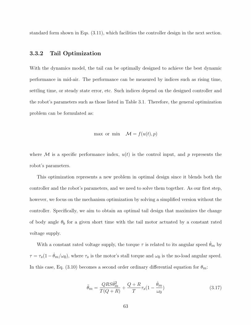
standard form shown in Eqs. (3.11), which facilities the controller design in the next section.

3.3.2 Tail Optimization

With the dynamics model, the tail can be optimally designed to achieve the best dynamic

performance in mid-air. The performance can be measured by indices such as rising time,

settling time, or steady state error, etc. Such indices depend on the designed controller and

the robot’s parameters such as those listed in Table 3.1. Therefore, the general optimization

problem can be formulated as:

max or min M = f(u(t), p)

where M is a specific performance index, u(t) is the control input, and p represents the

robot’s parameters.

This optimization represents a new problem in optimal design since it blends both the

controller and the robot’s parameters, and we need to solve them together. As our first step,

however, we focus on the mechanism optimization by solving a simplified version without the

controller. Specifically, we aim to obtain an optimal tail design that maximizes the change

of body angle θb for a given short time with the tail motor actuated by a constant rated

voltage supply.

With a constant rated voltage supply, the torque τ is related to its angular speed θm by

τ = τs(1− θm/ω0), where τs is the motor’s stall torque and ω0 is the no-load angular speed.

In this case, Eq. (3.10) becomes a second order ordinary differential equation for θm:

θm =QRSθ2

m

T (Q+R)+Q+R

Tτs(1−

θmω0

) (3.17)

63

From Eq. (3.17), we can solve θm(t). With θm(t), the body angle’s trajectory can be derived

from Eq. (3.9).

θb =

∫−Qx2 +H0

Q+R+ θb(0) (3.18)

where θb(0) is the initial angle for θb.

Using Eq. (3.17), we perform the optimal design in four steps: identifying optimization

variables, formulating the objective function, obtaining the constraints, and solving the

constraint optimization problem.

The parameters for the tail part design include mt, lt, It, and the speed reduction ratio

r between the motor gear and the tail gear (Fig. 3.2(c)). Since the carbon fiber rod in the

tail part has a negligible mass compared with the steel block, the tail’s moment of inertial It

can be approximated as It = mtl2t . Therefore, the optimization variables are mt, lt, and r.

Note that mb, lb, and Ib are known based on our previous jumping robot [99]. To simplify

the design, we choose the tail motor empirically (GH6123S from Gizmoszone) by estimating

the required torque and speed.

The objective function for the optimization problem is chosen to be the change of θb.

Specifically, an optimal design is one that maximizes the change of θb for a small fixed time

period (0.1 s) under a given constant rated voltage. To achieve this goal, we consider θb as

a function of mt, lt, and r from Eq. (3.17), and denote this function as θb(t) = f(mt, lt, r).

The optimization constraints are derived as follows. Since a large weight decreases the

jumping performance and increases the landing impact, we let mt ≤ 0.15mb. On the other

hand, since mt cannot be too small to perform effective aerial maneuvering, we constrain

mt ≥ 0.05mb. With similar practical reasons, let 0.75Lb ≤ lt ≤ 1.5Lb and 0.1 ≤ r ≤ 10 with

Lb = 7.5 cm being the maximum body length (Lb is different from lb in Fig. 3.4).

64

Based on the previous discussions, the optimal design problem is formulated as:

max θb(0.1) = f(mt, lt, r)

subject to 0.05mb ≤ mt ≤ 0.15mb, 0.1 ≤ r ≤ 10

0.75Lb ≤ lt ≤ 1.5Lb, θb(0) = constant

The optimization problem is solved using the Optimization toolbox in Matlab. Specifical-

ly, the fmincon function with the interior point algorithm is adopted. To avoid local minima,

we run the optimization algorithm 50 times with random initial points. For all of them, the

optimal result is mt = 1.3 g, lt = 6.8 cm, and r = 2.2. With the optimal parameters, θb

can change 80 degrees in 0.1 s. To accommodate the available off-the-shelf gears, we choose

r = 2. In this case, the value of θb(0.1) only decreases about 0.1%.

Based on the optimal design, the tail’s parameters are chosen as follows. The length of

the carbon fiber rod is lt = 6.8 cm, and the mass for the steel block is mt = 1.3 g. For the

gear train that actuates both the tail and the right wheeling gear (Fig. 3.2(c)), the motor

gear has 8 teeth, the tail gear has 16 teeth since r = 2, and the right wheeling gear has 28

teeth which is the same with the left wheeling gear.

3.4 Controller Design

In this section, a sliding mode controller is designed to regulate θb to θ∗b . Additionally, we

also discuss a special case to design a PD controller.

65

3.4.1 Sliding Mode Controller

Sliding mode control attains the control goal in two steps. First, the system’s trajectory

undergoes a reaching phase to a sliding surface. Second, the trajectory is constrained to the

sliding surface to approach the equilibrium during the sliding phase [108]. Let the sliding

surface be s = az1 + z2 with a > 0 a constant which determines the convergent speed during

the sliding phase.

As shown in the following, we have Q > 0 and the following two items are upper bounded

with the bounds denoted by k1 and k2, respectively:

∣∣∣∣TQ∣∣∣∣ ≤ k1,

∣∣∣∣Q2RS + ST (R−Q)

Q3

∣∣∣∣ ≤ k2

First we show that Q > 0. In fact,

Q = M − L cos θm ≥M − L = It +mtmblt(lt − lb)

mt +mb> 0

since lt is much larger than lb in our implementations. The bound for the first item |T/Q|

can be obtained as:

∣∣∣∣TQ∣∣∣∣ =

MN − L2 cos2 θmM − L cos θm

≤ MN

M − L:= k1

The bound for the second item is:

∣∣∣∣Q2RS + ST (R−Q)

Q3

∣∣∣∣ =|Q2RS + ST (R−Q)|

Q3≤ Q2|R||S|+ T |S||R−Q|

Q3

≤ (N + L)L

M − L+LMN |N −M |

(M − L)3:= k2

66

Based on the above results, we have the following theorem:

Theorem 1 The following controller can asymptotically stabilize the system represented by

Eq. (3.15) at the origin:

u = (ak1|z2|+ k2z22 + k3) sgn(az1 + z2) (3.19)

where k3 > 0 is a constant and sgn(·) is the sign function.

Proof 1 We first show that the system will reach the sliding surface. Define a Lyapunov

function as V = s2/2, then:

V = ss = s(a ˙z1 + ˙z2) = s(az2 + q) + pus

Since ∣∣∣∣az2 + q

p

∣∣∣∣ =

∣∣∣∣−aTQ z2 +Q2RS + ST (R−Q)

Q3z22

∣∣∣∣ ≤ ak1|z2|+ k2z22

we have

V ≤ |s||az2 + q|+ pus ≤ −p(ak1|z2|+ k2z22)|s|+ pus = k3p|s|

Since p = −Q/T < 0, we have V < 0 for any s 6= 0. Therefore, the system will reach the

sliding surface in finite time. After that, it will be governed by ˙z1 = −az1 to make the state

approach the origin.

The sliding mode controller in Eq. (3.19) only needs the feedback of transformed state

z1 = θb and z2 = θb, which are available from the gyroscope. Moreover, during the imple-

67

mentation, we can use a simplified controller

u = k sgn(az1 + z2) (3.20)

with k > ak1|z2| + k2z22 + k3. The stability for the system using this controller can also be

verified by showing V < 0.

3.4.2 Proportional-Derivative (PD) Controller

Besides the sliding mode controller, we examine the controller design for a special case

when lb = 0, which is detailed in [63]. This special case approximates the situation when

the robot has a very small lb such as the robots in [62] and [63]. In this case, since L =

mtmbltlb/(mt + mb) = 0, the dynamics equation (3.2) is simplified to Nθb = −τ . Since

N = Ib, the simplified system in state space form is thus:

˙z = Acz −Bcu/Ib (3.21)

For this system, a PD controller can be designed as:

u = IbKz (3.22)

where K = [Kp, Kd] is designed to make Ac −BcK Hurwitz.

Similar to the sliding mode controller, the PD controller only needs the feedback of the

transformed state. Therefore, we will include experimental results for the PD controller in

the next section since lb for our robot is close to zero.

68

(a) (b) (c)

Figure 3.5 Aerial maneuvering results from video frames show the robot trajectory in a singleimage for three cases. A schematic view for each robot in all the three images is added forillustration purposes. The dashed lines represent the tail, while the solid lines represent thebody. (a) the tail is not actuated; (b) the tail is controlled by the PD controller; (c) the tailis controlled by the sliding mode controller. Note that the robot jumps from right to left inthe figure.

3.5 Testing Results

With the designed robot, we first simulate the designed controllers and then conduct experi-

ments for aerial maneuvering. In addition, we also perform experiments for mode transitions.

3.5.1 Simulation Results for Aerial Maneuvering

We simulate the aerial maneuvering using Matlab/Simulink to validate the dynamics model

and controller design. Based on our robot design, the following parameter values are chosen

for the simulation: mt = 1.3 × 10−3kg, mb = 25.2 × 10−3kg, lt = 6.8 × 10−2m, lb =

1.0× 10−2m, It = 5.8× 10−6kg ·m2, and Ib = 1.0× 10−5kg ·m2.

The initial value for θb is chosen as 105, which means the robot takes off at an angle of

75. The initial value for θm is chosen as 180, which corresponds to the setup in experiments.

We let the desired body angle θ∗b = 30 to make the robot land on ground with one of the

69

two largest sides.

For the PD controller, we choose K = [240, 20]T to make the system approach θ∗b within

0.2 second. With all the parameters and the dynamics model, the trajectory of θb with

respect to time is obtained and shown by the solid line in Fig. 3.6.

For the sliding mode controller, we first calculate the bounds for the two items as: k1 =

2.2 × 10−5 and k2 = 1.96 × 10−6. The controller with saturation function is employed to

reduce the chattering

u = (ak1|z2|+ k2z22 + k3) sat(

az1 + z2

µ) (3.23)

where sat(·) is the saturation function and µ a positive constant [108]. Let a = 10, k3 =

5× 10−4, and µ = 1, which are chosen to make the response have a similar profile compared

with the PD controller. The trajectory of θb for the sliding mode controller is shown as the

dash line in Fig. 3.6.

Based on the simulation results, performances of the two controllers are compared and

major metrics are listed in Table 3.2. The sliding mode controller has a larger rising time

0.31s compared with 0.21s for the PD controller. However, if we consider the settling time as

when θb gets and stays within 10% of θ∗b , then the sliding mode controller settles faster. The

steady state errors for both controllers are zero, which verifies the stability of the system.

In addition, the PD controller has a larger percent of overshoot compared with the sliding

mode controller.

Table 3.2 Simulation results comparison for the two controllers

Metric PD controller Sliding mode controllerRising time (s) 0.21 0.31

Settling time (s) 0.37 0.26Steady state error (degree) 0 0Percent of overshoot (%) 18.66 4.56

70

0 0.2 0.4 0.6 0.8 120

30

40

50

60

70

80

90

100

110

Time (second)

θ b (de

gree

)

PD ControllerSliding Mode Controller

Figure 3.6 Simulation results for the PD controller and the sliding mode controller. Eachcurve shows the trajectory for θb with resect to time for each controller.

3.5.2 Experimental Results for Aerial Maneuvering

Based on the design presented in section 3.2, the robot prototype is built. With the prototype

and designed controllers, we conduct aerial maneuvering experiments to test the robot’s

performance.

The experiments are set up as follows. We let the robot jump in front of a white board

with height marks. To minimize the slippage during takeoff, the robot is placed on a sand

chapter to provide sufficient friction. Furthermore, the initial position of the tail is carefully

adjusted onto the top of the body so that the initial angular momentum can be minimized

at takeoff. Note that, however, the initial angular momentum cannot be eliminated as will

be explained in the experimental results.

All the sensing, computation, and control are implemented by C programming in the

embedded system discussed in section 3.2-B. The microcontroller, ATmega128RFA1, runs

71

at a speed of 8MHz. In each control loop, the microcontroller first samples raw angular

velocities from the gyroscope. Then it obtains the current roll, pitch, and yaw angle by

numerically integrating the angular velocity using the Runge-Kutta method. Based on the

current pitch angle, the control input is computed and the tail motor is actuated using the

computed control command. The time for one control loop is three millisecond, and the

system can achieve a bandwidth of 333Hz, which is sufficient for feedback control as will be

seen in the experimental results. Note that we neglect the drift problem for the gyroscope

since the control time for our experiment is less than one second.

Three sets of experiments are conducted. First, to compare with results under active

tail control, five jumping experiments with the tail disabled are performed. Second, five

experiments with active tail control using the PD controller are conducted. Third, another

five experiments using the sliding mode controller are carried out.

During each experiment, we use a Casio Exilim EX-ZR400 high-speed camera with a

frame rate of 240 frames/s to record the entire motion. Meanwhile, the body’s instantaneous

pitch, roll, and yaw angles—defined in Fig. 3.4—are recorded by the embedded control

system, which are sent back to a computer wirelessly after landing. The initial pitch angle

is obtained using the accelerometer. Since the roll and yaw angle cannot be controlled, we

only measure the change for each angle starting from an initial zero angle.

3.5.2.1 Jumping without Tail Actuation

For the five experiments without tail actuation, Fig. 3.5(a) shows the robot’s moving tra-

jectory for one of them (jump 2). In the trajectory, the time between each robot is 0.0625s.

Referring to the height marked on the left side of the white board, we visualize that the robot

jumps 32 inches (81.3 cm). Without actuating the tail, the robot’s pitch angle only changes

72

slightly due to a small initial angular momentum. The landing posture of the robot is bad

since landing on its feet may cause the robot to bounce severely on the ground, increasing

the probability of damage.

For jumping with the tail disabled, if there is no initial angular momentum and the air

resistance is neglected, the pitch, roll, and yaw angles should be constants all the time.

Fig. 3.7 shows the robot’s mid-air orientation for the five jumps, where the pitch, roll, and

yaw angles are plotted with respect to time. For all the jumps, the pitch angles do not change

too much since only a small initial angular momentum affects the pitch angles. In this case,

the pitch angles should change linearly; however, this is not the case in Fig. 3.7 because

the tail can slightly rotate even though it is not actuated due to the backlash between the

tail gear and the motor gear. From plot (b) and (c) in Fig. 3.7, the roll and yaw angles

change almost linearly in random manners. These imply that rotations about other axes

are affected by random initial angular momentums that the robot might have after takeoff.

Nevertheless, the changes in roll and yaw are relatively small, and they will not cause the

robot to flip around in mid-air to affect its landing posture significantly.

3.5.2.2 Aerial Maneuvering with the PD Controller

Experiments for tail actuated jumping are conducted as follows. Initially, the robot stands on

the ground, and the accelerometer obtains the initial pitch angle. Once the robot jumps up,

the accelerometer detects the free fall and triggers the controller to regulate the body’s pitch

angle to a desired value by swinging the tail. In mid-air, the gyroscope measures the body’s

instantaneous angular velocity, and the microcontroller calculates the body’s current angle

by numerical integrations. With the current angle, current angular velocity, and the desired

angle, the controller computes a voltage output for the tail motor to perform controlled aerial

73

maneuvering.

For the PD controller, we tune the values for Kp and Kd by letting the robot fall from

a given height since the dynamics is the same as the case when the robot jumps. Using the

Ziegler-Nichols tuning method, we obtain values for the controller as Kp = 40 and Kd = 0.3.

Fig. 3.5(b) shows one of the motion trajectories (jump 1) for the robot using the PD

controller. The time between each robot figure is 0.067s in the trajectory. Same to the

simulations, the desired angle of θb is set to be 30. From the trajectory, the robot rotates

its tail to regulate the pitch angle to 30. Eventually, the robot lands safely on a sponge pad

with one of its two large sides.

Fig. 3.8 shows the robot’s pitch, roll, and yaw angles with respect to time. Combining

Fig. 3.5(b) with Fig. 3.8(a), we observe that the tail rotates counter-clockwisely to make

the pitch angle θb approach 30, which is the horizontal yellow solid line in Fig. 3.8(a). The

system has a rising time about 0.2s, i.e., the pitch angle reaches 30 in 0.2s. After about 0.3s,

it reaches a steady-state value about 28, although a small oscillation exists. The reason for

this oscillation is that the smallest voltage applied to the tail motor is set to be the minimum

voltage which the motor overcomes its static friction. This means the motor will not stop

running even if the body has reached the desired angle. Additionally, the roll and yaw plots

in Fig. 3.8(b) and (c) provide information about rotations in uncontrolled axes. Unlike the

case when the tail is disabled, some experiments have nonlinear curves such as the yaw angle

for jump 3. The reason is that although the tail is only used to control the pitch angle,

manufacturing or assembly error may induce the cross coupling between the tail and yaw or

roll angle. Therefore, the rotation of the tail may slightly influence the change of yaw and

roll angle.

74

3.5.2.3 Aerial Maneuvering with the Sliding Mode Controller

Aerial maneuvering with the sliding mode controller is conducted similar to the one using the

PD controller. To simplify the parameter tuning process, we employ the simplified controller

in Eq. (3.20) with a saturation function sat(·)

u = k sat(az1 + z2

µ) (3.24)

where µ is a positive constant. Similar to the PD controller, we tune the parameters to

obtain good performances with the free-fall experiment, and the final parameters are chosen

as k = 255, µ = 600, and a = 50.

Five experiments are performed, and one (jump 4) of the robot’s trajectory is shown in

Fig. 3.5(c), with a time interval of 0.075s between each robot. As seen from the trajectory,

the robot lands on the ground safely with one of its two large sides. The three body angles

for five experiments are plotted in Fig. 3.9. From Fig. 3.9(a), the system has a rising time

about 0.3s, and the pitch angle θb oscillates around 30 thereafter. Compared with results

using the PD controller in Fig. 3.8, although the rising time is larger than the PD controller,

the sliding mode controller has a smaller overshoot and steady state error. Furthermore, the

oscillation after 0.3s is also smaller.

The robot also rotates in roll and yaw as can be seen from Fig. 3.9(b) and (c). Similar

to the reason for the PD controller, some of the curves for roll and yaw angle are nonlinear.

Nevertheless, these rotations do not significantly affect the landing posture of the robot.

75

Table 3.3 Experimental results comparison for the two controllers

Metric PD controller Sliding mode controllerRising time (s) 0.19 0.39

Settling time (s) 0.27 0.24Steady state error (degree) 2.00 0.22Percent of overshoot (%) 18.25 4.13

3.5.2.4 Comparison of the Two Controllers

To compare the results of the two controllers, we average the results of the five jumps for

each controller and plot the averaged result in Fig. 3.10. The data for important metrics

are also listed in Table 3.3. For the rising time, the PD controller reaches the desired angle

faster, which is the same to the simulation results shown in Table 3.2. The settling time for

both controllers, using the same definition for the simulation, is almost the same. However,

different from the simulation results, the PD controller has a larger steady state error, which

might be due to the discrete implementation of the controller. The percent of overshoot is

similar to the simulation results with the sliding mode controller having a smaller overshoot.

3.5.3 Tail Assisted Mode Transition

Besides aerial maneuvering, the tail is also designed for transition between wheeling and

jumping during the locomotion. But different from aerial maneuvering, the control of mode

transitions is achieved by wireless open loop control. Various commands can be sent from

a desktop computer wirelessly to the embedded system, which actuates the tail motor to

rotate the tail in different directions with specified speeds. Meanwhile, we visually check the

robot’s status to make sure it can finish the mode transition successfully.

As explained in the tail design part, the robot can utilize its tail to stand up for jumping

76

from the wheeling mode, and to lie down for wheeling from the jumping mode. Experimental

results for these two cases are elaborated in the following.

The first case is to let the robot stand up for jumping when the robot lies on the ground

with its side. One experiment for this case is shown in Fig. 3.11, where four frames from

a self-righting video are extracted with time labeled on the top right corner. In Fig. 3.11,

the robot is first in the wheeling mode with its wheels on the ground. Then, the robot’s tail

rotates towards the ground to make the robot’s wheels away from the ground. After that,

the robot starts to store energy and lower its center of mass in order to obtain a stabilizing

standing position later. At 12s, the robot is fully charged for jumping and the tail rotates

to push the ground such that the robot can complete the transition to a standing position

and be ready for taking off. Note that Fig. 3.11 only shows the self-righting from the side

with wheels. If the robot lands on the ground with the other side, the tail can rotate in the

opposite direction to perform self-righting as well.

The second case is transforming from the jumping mode to the wheeling mode. Fig. 3.12

shows one experimental result of such a transformation. Four frames are extracted from a

video that records the process. As shown in the figure, the lying down process is successfully

achieved by swinging the tail forward to push the ground, and the robot transforms to the

wheeling mode.

3.5.3.1 Wheeling and Turning

The wheeling and turning performances are also tested. In the wheeling experiment, the

robot is placed on a white board and beside a ruler in order to determine the wheeling

speed. The entire wheeling experiment is recorded by a camera. From the recorded video,

we obtain the instantaneous position of the robot in the horizontal direction every 0.36s

77

to create a position plot with respect to time, as shown in Fig. 3.13(a). The black circles

represent the experimental data and are connected by black dash lines between neighboring

circles. The red solid line is obtained by linear regression and its slope represents the average

linear speed—2.91 cm/s. The experimental data plot and the regression plot almost overlap

each other, which means the robot runs at an approximately constant speed.

The robot’s turning performance and the angular speed are also obtained from experi-

ments. We place the robot on a white board marked with a black straight line as a reference

position. Then the robot is controlled to turn, and we obtain the angle between the ref-

erence line and the robot’s tail every 0.3s. Fig. 3.13(b) shows the plot of the body angles

with respect to time for 360 turning. Similarly, the black circles are the experimental data

connected by black dash lines, and the red solid line is the projected plot given by linear

regression. We can see that the robot turns at a constant angular speed of 59/s.

3.6 Conclusions

In this chapter, we have presented the design, analysis, and experimentation of a miniature

tailed jumping robot (MSU tailbot) that uses an active tail to maneuver in mid-air for safe

landings. Additionally, the tailbot can wheel on the ground when no obstacle exists. The

mechanical and electrical designs of the tailbot are detailed. The dynamics model for the

tailbot in mid-air is established. Based on the dynamics model, the tail is optimized, and a

PD controller and a sliding mode controller are designed. Both simulation and experimental

results demonstrate successful aerial maneuvering using the two controllers. From the results,

the two controllers have comparable performances with the sliding mode controller having a

smaller steady state error in experiments. To the best of our knowledge, the tailbot is the

78

first centimeter scale robot that has all the three capabilities: jumping, wheeling, and aerial

maneuvering. With its small size and multi-mode locomotion ability, the tailbot can perform

energy efficient locomotion in environments with obstacles, which has many applications such

as mobile sensor networks, military surveillance, and environmental monitoring.

79

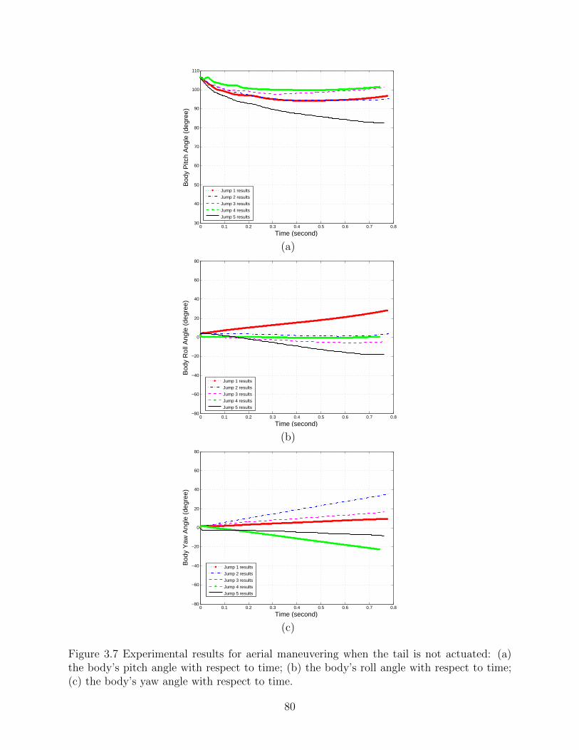
0 0.1 0.2 0.3 0.4 0.5 0.6 0.7 0.830

40

50

60

70

80

90

100

110

Time (second)

Bod

y P

itch

Ang

le (

degr

ee)

Jump 1 results

Jump 2 results

Jump 3 results

Jump 4 results

Jump 5 results

(a)

0 0.1 0.2 0.3 0.4 0.5 0.6 0.7 0.8−80

−60

−40

−20

0

20

40

60

80

Time (second)

Bod

y R

oll A

ngle

(de

gree

)

Jump 1 results

Jump 2 results

Jump 3 results

Jump 4 results

Jump 5 results

(b)

0 0.1 0.2 0.3 0.4 0.5 0.6 0.7 0.8−80

−60

−40

−20

0

20

40

60

80

Time (second)

Bod

y Y

aw A

ngle

(de

gree

)

Jump 1 results

Jump 2 results

Jump 3 results

Jump 4 results

Jump 5 results

(c)

Figure 3.7 Experimental results for aerial maneuvering when the tail is not actuated: (a)the body’s pitch angle with respect to time; (b) the body’s roll angle with respect to time;(c) the body’s yaw angle with respect to time.

80

0 0.2 0.4 0.6 0.8

20

40

60

80

100

120

Time (second)

Bod

y P

itch

Ang

le (

degr

ee)

Desired angleJump 1 resultsJump 2 resultsJump 3 resultsJump 4 resultsJump 5 results

(a)

0 0.2 0.4 0.6 0.8−60

−40

−20

0

20

40

60

Time (second)

Bod

y R

oll A

ngle

(de

gree

)

Jump 1 resultsJump 2 resultsJump 3 resultsJump 4 resultsJump 5 results

(b)

0 0.2 0.4 0.6 0.8−80

−70

−60

−50

−40

−30

−20

−10

0

10

Time (second)

Bod

y Y

aw A

ngle

(de

gree

)

Jump 1 resultsJump 2 resultsJump 3 resultsJump 4 resultsJump 5 results

(c)

Figure 3.8 Experimental results for aerial maneuvering when the tail is controlled by the PDcontroller: (a) the body’s pitch angle with respect to time; (b) the body’s roll angle withrespect to time; (c) the body’s yaw angle with respect to time.

81

0 0.2 0.4 0.6 0.8

20

40

60

80

100

120

Time (second)

Bod

y P

itch

Ang

le (

degr

ee)

Desired angleJump 1 resultsJump 2 resultsJump 3 resultsJump 4 resultsJump 5 results

(a)

0 0.2 0.4 0.6 0.8−60

−40

−20

0

20

40

60

Time (second)

Bod

y R

oll A

ngle

(de

gree

)

Jump 1 resultsJump 2 resultsJump 3 resultsJump 4 resultsJump 5 results

(b)

0 0.2 0.4 0.6 0.8

−60

−40

−20

0

20

40

Time (second)

Bod

y Y

aw A

ngle

(de

gree

)

Jump 1 resultsJump 2 resultsJump 3 resultsJump 4 resultsJump 5 results

(c)

Figure 3.9 Experimental results for aerial maneuvering when the tail is controlled by thesliding mode controller: (a) the body’s pitch angle with respect to time; (b) the body’s rollangle with respect to time; (c) the body’s yaw angle with respect to time.

82

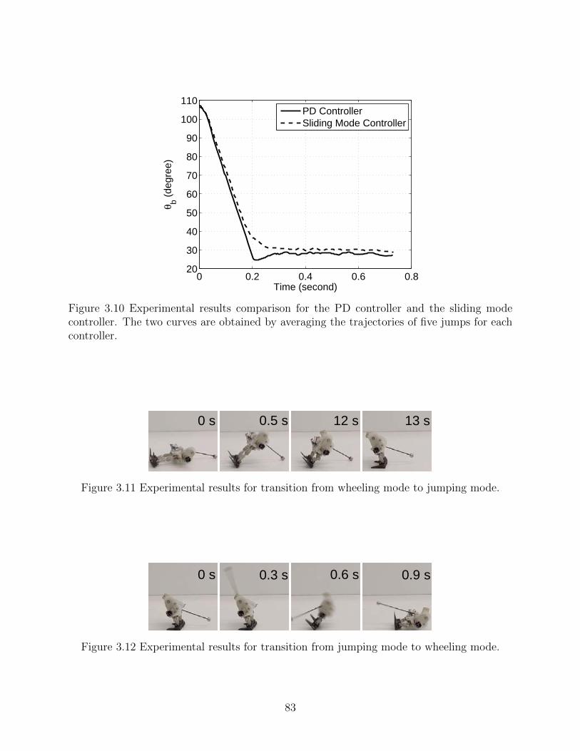
0 0.2 0.4 0.6 0.820

30

40

50

60

70

80

90

100

110

Time (second)

θ b (de

gree

)

PD ControllerSliding Mode Controller

Figure 3.10 Experimental results comparison for the PD controller and the sliding modecontroller. The two curves are obtained by averaging the trajectories of five jumps for eachcontroller.

0 s 0.5 s 12 s 13 s

Figure 3.11 Experimental results for transition from wheeling mode to jumping mode.

0 s 0.3 s 0.6 s 0.9 s

Figure 3.12 Experimental results for transition from jumping mode to wheeling mode.

83

0 1 2 3 40

2

4

6

8

10

12

Time (second)

Dis

tanc

e (c

m)

Experimental resultsProjected results

(a)

0 1 2 3 4 5 60

50

100

150

200

250

300

350

Time (second)

Ang

le (

degr

ee)

Experimental resultsProjected results

(b)

Figure 3.13 Running and turning experiments: (a) running experimental results and (b)turning experimental results.

84

Chapter 4

Non-vector Space Control: A

Biologically Inspired Control

Approach

4.1 Introduction

As discussed in the previous chapter, the MSU tailbot can use an active tail to control its

mid-air orientation to land on the ground safely [98, 109]. Specifically, the robot can land

with a specific orientation based on the feedback of its body angle from a gyroscope. Since

the gyroscope can only feedback a relative angle, the robot’s landing capability can only

be used in controlled and certain environments. In reality, however, small robots need to

interact with uncertain environments. For example, they may need to land on an unknown

surface in a specific manner. In this case, they need to rely on vision as a feedback mechanism

to achieve such a control goal.

As discussed in Chapter 1, small insects such as bees can achieve marvelous aerial ma-

neuvering such as landing or obstacle avoidance. In this chapter, we aim to investigate vision

based landing or perching on some surfaces without prior known orientation for small robots.

As shown in Fig. 4.1, the ultimate goal is to make the robot land on an arbitrary surface

85

N S C lNon-vector Space ControlControl goal: landing based on vision feedbackControl goal: landing based on vision feedback

A bee lands on a flower (Wikipedia) Robot lands on a tilted plane

E. Baird, et. al., “A universal strategy for visually guided landing,” Proceedings of National Academy of Sciences (PNAS), 110(46), pp. 18686‐18691, 2013.22

(a)

Robot

Unstructured Surface

(b)

Figure 4.1 Motivation for vision based robot control: (a) bees can land on an arbitrarysurface using vision feedback; (b) how can robots, with similar feedback mechanism, achievethe same feat?

with a given posture such as parallel to the surface using vision feedback. A novel non-vector

space approach will be used to obtain the control law. The approach will be implemented

on the MSU tailbot that can actively control the body’s mid-air orientation using the tail.

The vision based control method presented in this chapter belongs to the literature of vi-

sual servoing, which utilizes vision information to control the motion of a mechanical system.

For traditional image based visual servoing methods, prominent features are first extracted

from the image, and then a controller is designed to make the vector of feature positions

converge to a desired value [78]. Two possible issues associate with this feature based vec-

tor control method. On the one hand, robust feature extraction and tracking are difficult

in natural environments. In fact, most visual servoing experiments are based on artificial

fiducial markers [110]. On the other hand, feature extraction suffers from information loss

because only the feature information is used for control.

Different from the vision servoing methods which rely on feature extraction and tracking

during the control process, small insects perform vision based control without using features.

They generate control commands only based on two consecutive images obtained from theirs

86

eyes [44]. How could robots use such biological inspirations to achieve effective vision based

control?

We propose a non-vector space control method in this chapter. The general idea is to

form a set from an image and formulate the image dynamics in the space of sets. This space

is called the non-vector space because the linear structure in the vector space does not exist.

Based on the dynamics formulation, a controller can be designed directly on the image sets

for visual servoing. This non-vector space control method is different from existing direct

visual servoing methods because the problem formulation is different. Initial results for the

non-vector space controller have been reported in our previous research [111, 112].

The non-vector space control comes from a general framework called mutation analysis

for set evolutions, which is proposed by Aubin [113]. Mutation analysis provides a natural

way to describe various physical phenomena because some objects such as shapes and images

are basically sets. Since the introduction of mutation analysis, it has been investigated in

both theory and applications. On the theory side, it has been recently extended to obtain the

viability theorem for morphological inclusions [114] and the general morphological control

problems with state constraints [115]. On the application side, it has been applied to image

segmentation [116], visual servoing [117], and surveillance networks [118].

The visual servoing using mutational analysis is proposed by Doyen in [117]. Nevertheless,

possibly due to its abstract nature, no further extensions are performed afterwards. In this

chapter, we try to extend the results. The major extension can be summarized in two

aspects. First, the general framework for the non-vector space control is established in this

chapter which is not discussed in Doyen’s work. Second, the original formulation only deals

with binary images, while in this chapter, gray scale images are considered.

The schematic for the vision based robot control in the non-vector space is illustrated in

87

Non-vector Space Controller

Image Sensor

Goal Image

Current Image

RobotBody Rotation

Set Distance

Figure 4.2 Schematic for non-vector space control with the tailbot as an example

Fig. 4.2 with the MSU tailbot as an example. A goal image set corresponding to the desired

body orientation is first given. Based on the current image feedback, the non-vector space

controller will generate a control signal to drive the body to a desired orientation by swinging

the tail. At the new orientation, an updated current image will be obtained, and the same

process can be performed repeatedly until the body reaches the desired orientation. Note

that this schematic can also be applied to the general framework for visual servoing control

by replacing the tailbot in the figure with other mechanical systems.

The major contribution of this chapter can be summarized in two aspects. First, to

address the image based control, the direct visual servoing is implemented using the non-

vector space control. In this way, no feature extraction and tracking is needed. Second, the

general framework for the stabilization problem in the non-vector space is presented. The

framework can also be employed to stabilize other systems if the state for the system can be

represented as a set.

The rest of the chapter is organized as follows. First of all, the dynamics in the non-

vector space is introduced with tools from mutation analysis in section 4.2. After that, the

stabilization problem in the non-vector space is introduced in section 4.3, where the stabi-

88

lizing controller is designed. Then the stabilization controller is applied to visual servoing in

section 4.4. Finally, the testing results using a redundant robotic manipulator are given in

section 4.5 to validate the theory.

4.2 Dynamics in the Non-vector Space

Before the study of motion control problem with the non-vector space approach, the dynamics

should be first formulated. For robotic systems, the governing equation for the robot’s

motion can be modeled as a differential equation in the vector space. If the feedback image

is considered as a set, then this set evolves with the robot’s movement. In other words,

the differential equation for robot motion induces the set evolution. The evolution with

respect to time can be considered as the dynamics in the space of image sets. In this section,

the formulation of the dynamics equation in the non-vector space induced from a given

differential equation will be discussed.

The space of sets does not have the linear structure in the vector space because the

absence of addition and scalar multiplication [119]. Therefore, new tools from the mutational

analysis are employed [113]. With the mutation analysis, the time derivative of set evolutions

can be formulated. In fact, as will be shown later, the time derivative is the differential

equation inducing the set evolutions. With the time derivative, mutation equations in the

non-vector space, corresponding to differential equations in the vector space, can be obtained

to represent the set dynamics [113]. In the following, the detailed steps for the formulation

will be presented.

First of all, the space of sets is defined to form a metric space. Generally, the space,

denoted by P(Rn), is the power set of Rn, i.e., the collection of all subsets of Rn. Similarly,

89

if the dynamics is constraint to E ⊂ Rn, then the space is P(E). In P(Rn), we supply a

metricD : P(Rn)×P(Rn) 7→ R to define the distance between two sets. Any metric is valid if

it satisfies the three properties: symmetry, positive definiteness, and triangle inequality [120].

For example, the Hausdorff distance can be such a metric which is defined as follows.

Definition 1 Consider two sets X ⊂ Rn and Y ⊂ Rn, the distance from a point x ∈ X to

set Y is dY (x) = infy∈Y ||y− x|| with || · || representing the Euclidean norm. The Hausdorff

distance between X and Y is:

D(X, Y ) = max supx∈X

dY (x), supy∈Y

dX(y) (4.1)

The metric space supplied with metric D is denoted as (P(Rn), D). We also include the

definition of the projection from a point to a set for future use. The projection from x ∈ Rn

to Y ⊂ Rn is defined as PY (x) = y ∈ Y : ||y − x|| = dY (x), which includes all the points

in Y that are closest to x.

The gray scale image can be considered as a three dimensional set because each pixel has

two pixel index values and one intensity value. Since the cardinality of the set is finite, the

Hausdorff distance between two gray scale images X and Y is:

D(X, Y ) = max maxx∈X

miny∈Y||y − x||, max

y∈Yminx∈X||y − x||) (4.2)

where x, y ∈ N3 are vectors formed by three natural numbers. To interpret the distance

intuitively, one can consider each image as a surface in the three dimensional Euclidean

space, and the above definition is the Hausdorff distance between two surfaces.

90

4.2.1 Transitions

The set evolution with respect to time in a metric space is called tube. Formally, the tube

K(t) ⊂ Rn evolving in (P(Rn),D) is defined as: K(t) : R≥0 7→ P(Rn) where R≥0 is the set

of non-negative real numbers. In the case when gray scale images are the sets, the tube is

the surface evolution in the three dimensional space.

The transition is required for the definition of the time derivative for tubes. Let ϕ : E 7→

Rn with E ⊂ Rn be a bounded Lipschitz function. Denote the set of all such functions as

BL(E,Rn). For ordinary differential equation (ODE) x(t) = ϕ(x(t)) with initial condition

x(0) = x0. The transition for ϕ ∈ BL(E, Rn) at time t is defined as:

Tϕ(t, x0) = x(t) : x(t) = ϕ(x(t)), x(0) = x0 (4.3)

where x(t) is the solution to x(t) = ϕ(x(t)). In other words, the transition at time t is the

value of solution to a given ODE at the same time. Note that a rigorous definition for transi-

tions requires it to satisfy four conditions [119], but for simplicity, we use the above simplified

definition which can be shown to satisfy those four conditions (Ch. 1, Example 3, [119]). The

definition can be extended when the initial condition is a set instead of a point as stated in

the following definition:

Definition 2 The transition at time t for a function ϕ : E 7→ Rn with E ⊂ Rn starting

from an initial set K0 is:

Tϕ(t,K0) = x(t) : x(t) = ϕ(x(t)), x(0) ∈ K0 (4.4)

Since the initial conditions are in the set K0 instead of a single point, Tϕ(t,K0) is also a

91

set. In fact, Tϕ(t,K0) can be considered as a reachable set of points at time t according

to x = ϕ(x) with the initial points in K0. It is also a tube evolving from K0 according to

x = ϕ(x). Note that this definition also satisfies the four conditions for transitions (Ch. 1,

Example 4, [119]). In addition, the transitions discussed here is induced from differential

equations, and a general definition with differential inclusions can be defined as well [119].

To illustrate the idea of transitions, consider the case when x = [x1, x2]T and ϕ(x) =

[2, x1]T with the initial conditions in the set K0 = x : ||x|| < 1, which includes all the

points inside the circle shown in Fig. 4.3. In this case, the transition is:

Tϕ(t,K0) = x(t) :

x1

x2

=

2

x1

, x(0) ∈ K0

Solving the ODE, we can obtain the transition set at a given time t. For example, the

transition set Tϕ(1.5, K0), shown in Fig. 4.3, contains all the points inside the ellipse. Three

trajectories shown as dashed lines starting from points in K0 and ending with points in

Tϕ(1.5, K0) are also depicted.

−1 0 1 2 3 4

−0.5

0

0.5

1

1.5

2

2.5

3

3.5

4

K0

Tϕ

K0

Tϕ

K0

Tϕ

Figure 4.3 Illustration of the transition set

92

4.2.2 Mutation Equations

The transitions can be used to extend the time derivative of a function in the vector space

to the time derivative of a tube in a general metric space. In the vector space, the time

derivative for a function f(t) : R≥0 7→ Rn is defined as v = lim∆t→0[f(t + ∆t)− f(t)]/∆t.

This definition can be transformed to the first order approximation form, where the time

derivative v for f(t) should satisfy [119]:

lim∆t→0

1

∆t||f(t+ ∆t)− (f(t) + v∆t)|| = 0 (4.5)

where f(t) + v∆t can be considered as a new point in Rn obtained by starting from f(t)

and moving along the direction v after ∆t time. Similarly, in the metric space (P(E),D),

transition Tϕ(∆t,K(t)) can be considered as a new set in P(E) obtained by starting from

K(t) and moving along the ‘direction’ of ϕ ∈ BL(E, Rn) after ∆t time. Therefore, similar

to Eq. (4.5), ϕ satisfies the first order approximation of a tube K(t) if:

lim∆t→0+

1

∆tD(K(t+ ∆t), Tϕ(∆t,K(t))) = 0 (4.6)

where K(t+∆t) is the set at time t+∆t according to the tube K(t) : R≥0 7→ P(Rn). Based

on such an analogy from the vector space to the non-vector space, the derivative for a tube

called mutation can be defined. Since there may be none or multiple ϕ satisfying Eq. (4.6)

for a given tube, the mutation is a set defined as follows:

Definition 3 The mutation of a tube K(t), denoted as K(t), is defined as the set of all

93

ϕ ∈ BL(E, Rn) such that Eq. (4.6) is satisfied:

K(t) = ϕ(x) ∈ BL(E, Rn) : Eq. (4.6) is satisfied (4.7)

Based on the mutation of a tube, mutation equations in the non-vector space, the analogy

to differential equations in the vector space, can be defined as follows:

Definition 4 For a given function f : P(E) 7→ BL(E,Rn) mapping from a tube to a

bounded Lipschitz function, the mutation equation for the tube is defined as:

f(K(t)) ∈ K(t) with K(0) = K0 (4.8)

The solution to the mutation equation is the tube K(t) such that the function f(K(t)) ∈

BL(E,Rn) satisfies Eq. (4.6) at Lebesgue-almost every time.

A special case of the general mutation equation is the one induced by differential equa-

tions. Let x(t) = ϕ(x(t)) with ϕ(x(t)) ∈ BL(E, Rn), then the transition Tϕ(t,K0) can be

considered as a tube K(t) starting from K0. In this case, Eq. (4.6) is automatically satis-

fied because K(t + ∆t) = Tϕ(∆t,K(t)). Therefore, the mutation equation for this case is

ϕ(x(t)) ∈ K(t).

Since the tube K(t) is induced from ϕ(x(t)), it is tempted to write ϕ(x(t)) = K(t). This

is wrong because there may exist other bounded Lipschitz functions in K(t) except ϕ(x(t)).

For example, a stationary tube K(t) = x ∈ R2 : ||x|| ≤ 1 can be considered as being

induced from ϕ = [0, 0]T with K(0) = x ∈ R2 : ||x|| ≤ 1. Nevertheless, ϕ′ = [x2,−x1]T

94

also satisfies ϕ′ ∈ K(t). This can be seen by solving the ODE as:

x1 =√x1(0)2 + x2(0)2 sin[t+ arctan(x1(0)/x2(0))]

x2 =√x1(0)2 + x2(0)2 cos[t+ arctan(x1(0)/x2(0))]

where x1(0) and x2(0) are the initial conditions. From the solution, any trajectory starting

from x1(0) and x2(0) will stay on the circle x1(t)2 + x2(t)2 = x1(0)2 + x2(0)2. Therefore,

the transition Tϕ(∆t,K(t)) will be the same as K(t), which indicates ϕ′ = [x2,−x1]T is also

in the set K(t).

The mutation equation defined in Eq. (4.8) can be modified to add the control input to

the equation. Consider a map f : P(E)×U 7→ BL(E, Rn) where U is the set of all possible

controls u. Then the controlled mutation equation can be defined as:

f(K(t), u(t)) ∈ K(t) with u(t) = γ(K(t)) (4.9)

where γ : P(E) 7→ U is the feedback map from the current set K(t) to the control input.

Similar to the special case of mutation equation, if the tube is induced from a controlled

differential equation ϕ(x(t), u(t)) ∈ BL(E, Rn), then the controlled mutation equation can

be written as ϕ(x(t), u(t)) ∈ K(t) with u(t) = γ(K(t)).

4.3 Stabilization Control in the Non-vector Space

With the dynamics modeling in the non-vector space, the stabilization problem can be

discussed. In this section, the problem will be formulated and the stabilizing controller

design will be presented.

95

4.3.1 Stabilization Problem

Before the design of the stabilizing controller, the stability in the non-vector space (P(E),D)

should be defined. Similar to equilibrium points, the equilibrium set for mutation equation

f(K(t)) ∈ K(t) is defined as a set K ⊂ E such that f(K) = 0. Based on the metric D,

the stability for a mutation equation around an equilibrium set can be defined similarly to

equilibrium points in the vector space [121].

Definition 5 Suppose in (P(E),D), the mutation equation f(K(t)) ∈ K(t) with f : P(E) 7→

BL(E,Rn) and K(0) = K0 has an equilibrium set K ⊂ E. Then

• K is stable if for any ε > 0, there exists δ = δ(ε) > 0 such that

D(K0, K) < δ =⇒ D(K(t), K) < ε

• K is unstable if it is not stable

• K is asymptotically stable if it is stable and there exists δ such that

D(K0, K) < δ =⇒ limt→∞

D(K(t), K) = 0

• K is exponentially stable if there exist positive constants c, k, and λ such that:

D(K(t), K) ≤ kD(K0, K)e−λt,∀ K withD(K0, K) < c

In the above definitions, the general norm in the vector space is replaced by the metric

distance between K(t) and K. Based on the definitions, the stabilization problem for the

96

controlled mutation equation (4.9) can be formulated.

Stabilization Problem: Assume a system in (P(E),D) is described by the controlled

mutation equation f(K(t), u(t)) ∈ K(t) with an initial set K0. Given a goal set K in the

neighborhood of K0, design a feedback controller u(t) = γ(K(t)) based on the current set

K(t) such that K is stable, asymptotically stable, or exponentially stable.

The above stabilization problem cannot be addressed using existing theories in the vector

space due to the lack of linear structure in the non-vector space. Nevertheless, the Lyapunov

theory, if properly extended to the non-vector space, can be adopted for the stability analysis

of a given system.

4.3.2 Lyapunov Function Based Stability Analysis

Since the state in the non-vector space is a set, the Lyapunov function is a function of sets

instead of vectors. Such functions are also called shape functionals in the shape optimiza-

tion [122]. To deal with the functionals, the Lyapunov function can be defined as bounded

by a given real valued function stated as follows:

Definition 6 For the system f(K(t)) ∈ K(t) with K(0) = K0 and an equilibrium set K,

let V : P(E) 7→ R≥0 be a shape functional, and φ : R 7→ R be a continuous function. Then

V is a φ-Lyapunov function for the system if the following two conditions are satisfied:

• V (K) = 0 and V (K(t)) > 0 for K(t) 6= K;

• V (K(t)) ≤ h(t), ∀ t ≥ 0 with V (K0) = h(0), where h(t) is the solution to the differen-

tial equation h = φ(h).

From the above definition, we see that if h(t) converges to zero, then V (K(t)) will also

converge to zero. V (K(t)) represents the trajectory along the solution tube K(t). Note that

97

a similar definition exists in [123]; however, our definition incorporates the equilibrium set

in order to discuss the stability problem systematically. With the definition of the Lyapunov

function, the stability of the system in the non-vector space can be determined as stated in

the following theorem:

Theorem 2 For the system f(K(t)) ∈ K(t) with K(0) = K0 and an equilibrium set K, if

there exists a continuous function φ : R 7→ R and the corresponding φ-Lyapunov function

V : P(E) 7→ R≥0. Without loss of generality, let the equilibrium point for h = φ(h) be zero,

then K is

• stable if zero is stable for h = φ(h);

• asymptotically stable if zero is asymptotically stable for h = φ(h);

• exponentially stable if zero is exponentially stable for h = φ(h).

Proof: Let D((K(t), K) = |V (K(t)) − V (K)| = |V (K(t))|. If K is fixed, then one can

verify that such a definition satisfies the three metric properties. Therefore, it can be used

as a metric in Definition 5 for the proof.

Stability: for any ε > 0, by the stability of zero for h = φ(h), there exists δ(ε) > 0

such that |h(0)| < δ =⇒ |h(t)| < ε. With the same δ, we have D(K(t), K) = |V (K(t))| =

V (K(t)) ≤ h(t) < ε for D(K0, K) = |V (K0)| = |h(0)| < δ.

Asymptotical stability: by the asymptotical stability of zero for h = φ(h), there exists δ > 0

such that |h(0)| < δ =⇒ limt→∞ |h(t)| = 0. With the same δ, we have limt→∞D(K(t), K) =

limt→∞ |V (K(t))| ≤ limt→∞ |h(t)| = 0. Therefore, we have limt→∞D(K(t), K) = 0 for

D(K0, K) = |V (K0)| = |h(0)| < δ.

Exponential stability: by the exponential stability of zero for h = φ(h), there exist positive

constants k and λ such that |h(t)| = k|h(0)|e−λt for any |h(0)| < c. With the same k

98

and λ, we have D(K(t), K) = V (K(t)) ≤ h(t) = k|h(0)|e−λt = kD(K0, K)e−λt for any

D(K0, K) = |h(0)| < c.

With the above theorem, the next question is how to find or construct the desired Lya-

punov function. The answer to this question requires the definition of derivative for shape

functionals.

Definition 7 [122] Given a shape functional V : P(E) 7→ R, a set K ∈ P(E), and a

function ϕ ∈ BL(E,Rn). Then V has a Eulerian semiderivative Vϕ(K) at K in the direction

of ϕ if

lim∆t→0+

V (Tϕ(∆t,K))− V (K)

∆t

exists and is finite.

Note that the definition is similar to the derivative for a function in the vector space

because Tϕ(∆t,K) is a new set starting from K in the direction ϕ after ∆t time. With

this definition, the Lyapunov functions in the non-vector space can be characterized by the

following theorem:

Theorem 3 [123] Consider a map f : P(E) 7→ BL(E, Rn). Let V : P(E) 7→ R≥0 be

a shape functional which has a Eulerian semiderivative in the direction of f(K). Assume

φ : R 7→ R≥0 be a continuous function. Then V is a φ-Lyapunov function if and only if:

Vf(K)(K) ≤ φ(V (K)) (4.10)

for any K in the domain of V .

The proof of this theorem can be found in [123]. This theorem can be applied to the controlled

mutation equation to design stabilizing controllers. The general procedure is similar to the

99

case in the vector space. First of all, a Lyapunov function candidate is found, which can

be the distance function between two sets. Then the shape directional derivative for the

Lyapunov function is obtained. Finally, a controller can be designed to satisfy the inequality

(4.10). Depending on the function φ for the Lyapunov function, the stability, asymptotical

stability, or exponential stability can be guaranteed.

4.3.3 Stabilizing Controller Design

With the Lyapunov theory in the non-vector space, the stabilization controller can be de-

signed for the system with image feedback described by the controlled mutation equation

Eq. (4.9). In this sub section, we consider a more general case corresponding to the time

invariant linear system. In this case, the mutation equation is induced from the differential

equation x = Ax + Bu with x ∈ Rn, u ∈ Rm, A ∈ Rn×n, and B ∈ Rn×m. Therefore,

the controlled mutation equation is Ax + Bu ∈ K. Note that the time t is omitted for

clear presentation. For such a system, the following Lyapunov function candidate can be

used [117]:

V (K) =1

2

∫Kd2K

(x)dx+1

2

∫Kd2K(x)dx (4.11)

With such a candidate, the first condition required for a Lyapunov function in Defi-

nition 2 can be verified. For the second condition, the controller should be designed for

the verification. In fact, a stabilizing controller can be designed as stated in the following

theorem:

Theorem 4 For the system Ax+Bu ∈ K(t) with x ∈ Rn, u ∈ Rm, A ∈ Rn×n, B ∈ Rn×m,

and K ⊂ Rn, the exponential stability for a given desired set K can be achieved by the

100

following controller:

u = −E(K)(αV (K) +H(K)

||E(K)||2) (4.12)

where α > 0 is a gain factor. H(K) is a scalar and E(K) ∈ Rm is column vector defined by:

H(K) =1

2

∫K

[d2K

(x)trace(A) + (Ax)T(x− PK

(x))]dx−∫K

(APK(x))T(x− PK(x))dx

E(K) = BT[

∫K

(x− PK

(x))dx−∫K

(x− PK(x))dx]

where trace(A) is the trace for matrix A.

Note that the time t is also omitted for clear presentation. To prove this theorem, the

following two lemmas for the Eulerian semi-derivative of the two components in the Lyapunov

function candidate are needed.

Lemma 1 [117] For a function ϕ ∈ BL(E,Rn), the Eulerian semiderivative for V 1 =

1

2

∫K d2

K(x)dx at K in the direction of ϕ is:

V 1ϕ (K) =

∫K

[1

2d2K

(x)div(ϕ) + ϕ(x)T(x− PK

(x))]dx

where div(·) is the divergence of a function.

Lemma 2 [117] For a function ϕ ∈ BL(E,Rn), the Eulerian semiderivative for V 2 =

1

2

∫Kd2K(x)dx at K in the direction of ϕ is:

V 2ϕ (K) =

∫K−ϕ(PK(x))T(x− PK(x))dx

Proof of Theorem 4: The proof of this theorem is based on theorem 2, theorem 3, and

101

the previous two lemmas. Let ϕ = Ax+Bu, then with the above two lemmas, we have:

Vϕ(K) =V 1ϕ (K) + V 2

ϕ (K)

=1

2

∫K

[d2K

(x)trace(A) + (Ax)T(x− PK

(x))]dx−∫K

(APK(x))T(x− PK(x))dx+

uTBT[

∫K

(x− PK

(x))dx−∫K

(x− PK(x))dx]

=H(K) + uTE(K)

Therefore, if u = −E(K)(αV (K) + H(K)/||E(K)||2), then Vϕ(K) = −α||E(K)||2V (K).

From theorem 3, V (K) is a Lyapunov function for φ(h) = −βh with β a constant satisfying

0 < β ≤ α||E(K)||2. Based on theorem 2, the exponential stability can be achieved since the

equilibrium point zero for h = φ(h) = −βh is exponential stable.

4.4 Application to Visual Servoing

The visual servoing problem can be modeled by the special system in the Theorem 4, and

the controller can be readily applied. In fact, for servoing with grey scale images, each

pixel can be represented by a three dimensional vector x = [x1, x2, x3]T where x1 and x2

are the pixel indices, and x3 the pixel intensity. For a general visual servoing problem, the

control input is the camera’s spatial velocity. Therefore, the control input u(t) has three

translational components and three rotational components, which can be represented by a

vector u(t) = [vx, vy, vz, ωx, ωy, ωz]T.

The system in Theorem 4 is determined by ϕ(x), which is further determined by the

relationship between u(t) and x(t). The perspective projection sensing model in computer

vision can be used to derive such a relationship. Under constant lighting condition, x3 will

102

be a constant for each pixel; therefore, x3 = 0. With a unit camera focal length, a 3D point

with coordinates P = [px, py, pz]T in the camera frame will be projected to the image plane

with coordinates:

x1 = px/pz x2 = py/pz (4.13)

Based on these equations, the relation between u(t) and x(t) can be obtained as:

x(t) = L(x(t))u(t) (4.14)

where

L =

−1/pz 0 x1/pz x1x2 −(1 + x2

1) x2

0 −1/pz x2/pz 1 + x22 −x1x2 −x1

0 0 0 0 0 0

Note that first two rows are the same as the interaction matrix in visual servoing [78]. In

Eq. (4.14), x(t) = ϕ(x(t), u(t)) = L(x(t))u(t) is linear in u; therefore, the controller in

Eq. (4.12) can be applied by letting A = 0 and consider B as a non-constant. Specifically,

we have the following theorem

Theorem 5 [112] For the system described by the following set dynamics

ϕ(z(t), u(t)) = L(z(t))u(t) ∈ K(t) with K(0) = K0 (4.15)

where L(z(t)) ∈ Rp×q, z(t) ∈ K(t) ⊂ Rp, u(t) ∈ Rq, and ϕ(z(t), u(t)) ∈ BL(E,Rp), the

following controller can locally asymptotically stabilize it at a desired set K:

u = γ(K) = −αD(K)+ (4.16)

103

where α ∈ R>0 is a gain factor, and D(K)+ is the Moore-Penrose pseudoinverse of D(K),

which is a column vector

D(K) =1

2

∫Kd2K

(z)(

p∑i=1

∂Li∂zi

)Tdz+

∫KL(z)T(z−P

K(z))dz−

∫KL(PK(z))T(z−PK(z))dz

(4.17)

where Li (i = 1, 2, . . . , p) is the i-th row vector in matrix L, and ∂Li/∂zi is also a row vector

with the same dimension.

The preliminary experiments for two cases will be carried out to verify the controller

in the experimental part. For easy implementation, the simplified controllers for these two

cases will be obtained.

4.4.1 3D Translation

In this case, the camera can only perform the translational motion. The row vector D(K)

can be simplified to:

D(K) =

∫K

1

pz[0, 0, d2

K(x)]dx+

∫K

1

pz(x− P

K(x))TL(x)dx

−∫K

1

pz(x− PK(x))TL(PK(x))dx (4.18)

with

L(x) =

−1 0 x1

0 −1 x2

0 0 0

In general, pz varies with different x in the set K. A special case is when the observed object

is planar, then pz will be the same for all x ∈ K, and it can be taken out from the integral.

104

In this case, although pz will change during the translation along the optical axis, it only

effects the magnitude of u(t). Therefore, we can assume pz to be one.

4.4.2 SE(2) Motion

In this case, the camera has three degree-of-freedom (DOF). In addition to 2D translational

movement, it can also rotate about its optical axis. The row vector D(K) can be simplified

to:

D(K) =

∫K

(x− PK

(x))TL(x)dx−∫K

(x− PK(x))TL(PK(x))dx (4.19)

with

L(x) =

−1/pz 0 x2

0 −1/pz −x1

0 0 0

Note that pz will be a constant if a planar object is used.

4.5 Testing Results

Although the ideal case is to use the tailed jumping robot for experimental results, as our

initial step to validate the non-vector space control theory, we apply the approach to robot-

ic manipulators [112]. Note that this approach has been also verified using atomic force

microscope images [111].

The detail experimental framework is shown in Fig. 4.4, which is the general look-and-

move structure [124]. First of all, the non-vector space controller generates a camera velocity

based on the current image from the camera and the goal image. This velocity is resolved

into the joint speeds via the inverse velocity kinematics. Then the robot executes this speed

105

through the robot controller until a new joint speed command is received. Note that we use

an eye-in-hand configuration with the camera attached to the manipulator’s end-effector.

The key step in Fig. 4.4 is the inverse velocity kinematics, which is well discussed in

standard robotics textbooks for a six DOF manipulator [125]. Nevertheless, we will use a

seven DOF manipulator to provide flexibility and capacity by its redundancy. In this case,

the redundancy resolution requires extra efforts which will be briefly described in this section.

Manipulator with a camera on end effector

Joint motor speed

controller

Inverse veolocity

kinematics

Non-vector space

controller

Joint variable feedback

Desired image

Image feedback

Camera velocity

Jointspeed Motor

Input

Camera

Figure 4.4 The implementation framework to verify the non-vector space controller

The LWA3 redundant manipulator with seven revolute joints from Schunk is used for

experiment. In order to resolve the redundancy, an extra variable is introduced. It is named

arm angle and denoted by φ. It represents the configuration of the plane constructed by the

elbow-shoulder link and elbow-wrist link with respect to the shoulder-wrist axis [126]. Let

ξee ∈ R6 be vector for the three linear and three angular velocities of the end-effector. Let

θ ∈ R7 denote the seven joint angles of the manipulator. Then ξee and θ has the following

relationship:

ξee = Jee(θ)θ (4.20)

where Jee(θ) ∈ R6×7 is the Jacobian matrix of the end-effector. The arm angle φ introduced

earlier is related to the seven joint angles by:

106

φ = Jφ(θ)θ (4.21)

where Jφ(θ) ∈ R1×7 can be considered as the Jacobian matrix of the arm angle.

Eqs. (4.20) and (4.21) can be combined together to obtain:

Y ,

ξee

φ

=

Jee(θ)

Jφ(θ)

θ = J(θ)θ (4.22)

where J(θ) ∈ R7×7 is the augmented Jacobian matrix of the full configuration. Since J(θ) is

a square matrix, a unique velocity for the seven joints can be obtained if J(θ) is nonsingular.

In this way, the redundancy problem is solved.

With above redundancy resolution, we can obtain the joint speed given the end-effector’s

velocity in the end-effector frame. But the output of the non-vector space controller is the

velocity of the camera in the camera frame. Therefore, the transformation from the camera

frame to the end-effector frame should be derived. Denote the camera velocity with ξc ∈ R6.

Then we have

ξee = Jceξc (4.23)

where Jce ∈ R6×6 is the transformation matrix which can be obtained once the spatial

relationship between the camera and end-effector is known [125]. From Eqs. (4.22) and

(4.23), the relationship between the joint velocity and the camera velocity is:

Y ,

ξc

φ

=

J−1ce Jee(θ)

Jφ(θ)

θ = J(θ)θ (4.24)

where J(θ) ∈ R7×7 is the augmented Jacobian matrix of the new full configuration. Because

107

the manipulator has seven DOF, the three position and three orientation movements of the

camera are all achievable. Therefore, we can let camera’s velocity be the output of the

non-vector based controller:

ξc = u(t) (4.25)

To achieve this output, the joint velocities of the manipulator can be obtained by the

inverse velocity kinematics of Eq. (4.24):

θ = J−1(θ)Y (4.26)

where the velocities of the camera are obtained from Eq. (4.25). The velocity of the arm an-

gle is determined by the online sensors for obstacle avoidance of the manipulator links [127].

Then the joint velocities are executed by the joint motors based on joint motor speed con-

trollers.

To validate the non-vector space controller, experiments are conducted on the LWA3

redundant manipulator. The experimental setup is shown in Fig. 4.5, where an ordinary

CMOS camera is rigidly attached to the end-effector. As our preliminary experiment, a

planar object with a rectangle, a circle, and a triangle printed on a white paper is placed

on the ground. Note that although planar geometric shapes are used, no image feature

extraction and tracking are performed in the experiments.

As the quality of the CMOS camera is poor, the image noise can be quite large. For

example, with two consecutive images obtained with a still camera looking at a still envi-

ronment, the variation of image intensities may be up to 12%. To address this issue, we

convert grey scale images to binary images for our experiment. A 120 × 160 grey scale im-

108

Camera

Figure 4.5 Experimental setup to verify the non-vector space controller

age is obtained, then it is converted to a binary image to retain the geometric shapes. The

camera is calibrated, and the following intrinsic parameters are found: focal lengths in pixels

fx = fy = 204 and principle points in pixels ur = 48, and uc = 92.

Experiments for two subsets of rigid motion discussed are carried out. The general process

for the experiments is as follows. First of all, the manipulator is moved to a desired position,

where a desired image is acquired. The desired position is obtained using the manipulator’s

forward kinematics. Then the manipulator is moved to some initial position, where the initial

image is recorded. Then the manipulator will start moving according to the framework in

Fig. 4.4. During the movement, the manipulator end-effector’s positions are recorded with

5Hz frequency. In this way, the error trajectory can be obtained after the experiment.

4.5.1 3D Translational Motion

In this experiment, the manipulator is allowed to move in all the three translational di-

rections. Four experiments are carried out, and the detail of one experiment is shown in

Fig. 4.7. The meaning for each figure is the same to the 2D translation case. As discussed

109

(a) Desired Image (b) Initial Image

Figure 4.6 Initial and desired image for the 3D translation

0 10 20 30 40−80

−60

−40

−20

0

20

40

60

80

Time(s)

Err

or (

mm

)

Error in xError in yError in z

(a) Error in the task space

0 10 20 30 400

0.05

0.1

0.15

0.2

0.25

0.3

0.35

Iterations

Hau

sdor

ff D

ista

nce

(pix

el)

(b) Hausdorff distance

Figure 4.7 Experimental results for the 3D translation

before, we can use a constant depth pz in the controller for planar objects. From the results,

we see that the controller can make the manipulator move to the desired position.

Table 4.1 Results for 3D translation

Trial No. 1 2 3 4 average

Final Errorx (mm) 2.4 2.1 2.5 1.3 2.1y (mm) 0.8 1.9 1.5 2.9 1.8z (mm) 2.1 3.3 0.1 0.6 1.5

The final errors in three directions for the four experiments are shown in table 4.1.

The average errors are also computed, and the results show performance similar to the 2D

translation case.

110

(a) Desired Image (b) Initial Image

Figure 4.8 Initial and desired image for the SE(2) motion

0 10 20 30 40−40

−20

0

20

40

60

80

100

Time(s)

Err

or (

mm

or

degr

ee)

Error in xError in yError in θ

(a) Error in the task space

0 10 20 30 40 500

0.05

0.1

0.15

0.2

0.25

0.3

0.35

0.4

Iterations

Hau

sdor

ff D

ista

nce

(pix

el)

(b) Hausdorff distance

Figure 4.9 Experimental results for the SE(2) motion

4.5.2 SE(2) Motion

In this experiment, the manipulator can perform the 2D translation and a rotation about

its optical axis. Four experiments are conducted, and one result is shown in Fig. 4.9. Note

that the rotation error is also plotted in Fig. 4.9(a) with degree as the unit. From the plot,

there are some overshoots for the system, but the controller can still stabilize the system at

the desired position.

The final errors for the four experiments are shown in table 4.2, where the unit for the

rotation is degree. From the table, we see that the error in rotation is quite small.

111

Table 4.2 Results for SE(2) motion

Trial No. 1 2 3 4 average

Final Errorx (mm) 1.7 1.0 0.8 0.7 1.1y (mm) 0.4 2.7 2.7 0.7 1.6θ () 0.01 0.32 0.41 0.83 0.39

4.6 Conclusions

In this chapter, a bio-inspired non-vector space approach is presented. The control method

formulates the system dynamics in the space of sets. Due to the lack of linear structure

in such a space, new tools from the mutational analysis are employed. The Lyapunov

theory can also be extended in such a space. Based on the dynamics and Lyapunov theory,

the stabilization problem is proposed and a stabilizing controller is designed for a general

system. The designed controller is applied to vision based control. The testing results using

a redundant robotic manipulator demonstrate the effectiveness of the controller to steer the

current image set to a desired image set.

112

Chapter 5

Compressive Feedback based

Non-vector Space Control

5.1 Introduction

Although the non-vector space control approach discussed in the previous chapter can be

used for vision based control of robot’s landing postures, the vision feedback from vision

sensor has a large amount of data, which cannot be handled by meso-scale robots such as

the tailbot, which has a limited computation power [88].

We can alleviate this problem by reducing the number of samples. A smaller number of

samples, however, may lose information in the original image. This problem can be addressed

by the recently breakthrough in signal processing: the compressive sensing. In essence,

instead of sampling the entire signal, compressive sensing directly samples the signal in its

compressed form. In this way, the number of samples can be drastically reduced compared

to the original image size. After the sampling, the original image can be recovered using

advanced optimization algorithms [128].

In previous works, the compressive sensing and non-vector space control are discussed

separately in signal processing and control society, respectively. In this chapter, we propose

the idea of compressive feedback. Furthermore, we aim to apply the compressive feedback

to the non-vector space control approach: the compressive feedback based non-vector space

113

control method [129]. In other words, we directly used the compressive feedback as the input

to the non-vector space controller to achieve the control goal. The general structure of the

proposed method is shown in Fig. 5.1. A reference input (goal set) is given in the form of

compressive representation. Then based on the current compressive feedback, the non-vector

space controller will generate a control signal to correct the error between the compressive

goal set and the compressive feedback.

Non-vector Space Controller

Compressive Goal Set

Sensor

Plant

Compressive Feedback Set

Figure 5.1 Schematic for non-vector space control with compressive feedback

The concept of compressive sensing has been introduced to control systems in recent

years [129, 130]. The observability matrix is analyzed in the framework of compressive sensing

and the observability and identification of linear system are discussed in [131] and [132].

The observability problem is also recently discussed in [133] for linear systems. With a

different motivation, the compressive sensing is used to sparsify the system states, and then

the recovered states are used for feedback [134]. The idea of sparsity is also employed

in [135, 136] to solve the network control problem with rate-limited channels. However, all

of the feedbacks used in these approaches are still regular state/output feedbacks. The only

difference is that they are recovered from compressive sensing instead of direct sensing. In

contrast, we intend to directly use the compressive data as the feedback without recovering.

The rest of this chapter is structured as follows. First of all, the mathematical prelimi-

naries will be discussed in section 5.2, where the basics for compressive sensing are reviewed.

114

After that, the stabilizing controller design based on full feedback and compressive feedback

are discussed in section 5.3. With the designed controller, the stability analysis is performed

for sparse and approximate sparse feedback in section 5.4. Finally, applications to visual

servoing for robotic manipulations are discussed in section 5.5.

5.2 Mathematical Preliminaries

The work presented in this chapter relies on the compressive sensing to develop compressive

feedbacks. We review the basics for compressive sensing in this section.

The notations in this chapter are as follows. R, R>0, and R≥0 represent the set of real,

positive real, and nonnegative real numbers, respectively. P(Rp) denotes the powerset of

Rp; that is, the collection of all the subsets in Rp. Similarly, P(E), with E ⊂ Rp, is the

powerset of E. Unless otherwise stated, || · || denotes the Euclidean norm of a vector.

Compressive sensing is a new paradigm to acquire signals. Traditional signal acquisition

methods sample the signal based on the Shannon-Nyquist theorem. After the sampling, the

signal is compressed for storage or transmission. In contrast, the compressive sensing directly

samples the signal in its compressed form [137]. Then it relies on convex optimization or

greedy algorithms to recover the original signal. Again, we only include the essentials here

for the sake of completeness, and a recent comprehensive introduction can be found in [138].

Suppose an unknown finite dimensional signal x ∈ Rn is sampled in the compressed form

y ∈ Rm with m n through a measurement matrix Φ ∈ Rm×n, that is

y = Φx (5.1)

115

Then, x can be faithfully recovered from y using tractable numerical algorithms if x and Φ

satisfy some general conditions, which we will elaborate in the following discussions.

For the original signal x, it should be sparse or approximately sparse, or have a sparse

or approximately sparse representation in some basis. A vector x ∈ Rn is S-sparse if the

number of nonzero elements of x is at most S. Denote all the S-sparse vectors by ΩS

ΩS = x ∈ Rn : ||x||0 ≤ S

where ||x||0 is the number of non-zero elements for x [138].

In some cases, x ∈ Rn may not be sparse itself but sparse in some orthonormal basis.

Let Ψ ∈ Rn×n be such a basis. In this case, x can be expanded in Ψ as follows

x = Ψx, with x ∈ ΩS

The exact S-sparse, however, cannot be achieved in practical signals. In most situations, the

signals can be well approximated by an S-sparse signal. The following definition quantifies

such approximately sparse signals.

Definition 8 The best S-sparse approximation for a vector x ∈ Rn is a vector xS ∈ ΩS

such that

||x− xS || ≤ ||x− x||, ∀ x ∈ ΩS

Note that xS can be obtained by retaining the S largest elements in x and setting the

other elements to zero. If ||x−xS || is small enough, then x is well approximated by xS , and

we say x is an approximately sparse signal.

If x is sparse or approximately sparse in some orthonormal basis Ψ, the compressive

116

sensing problem can be written as

y = ΦΨx (5.2)

Let A = ΦΨ, which is the new measurement matrix. With Eq. (5.2), the original signal can

be obtained from x = Ψx after x is recovered from y.

Besides the sparse requirement for the original signal, the measurement matrix should

also satisfy some condition for recovering x from y in Eq. (5.1) or x from y in Eq. (5.2). One

of such conditions is the restricted isometry property.

Definition 9 A matrix A ∈ Rm×n with m < n satisfies the restricted isometry property

(RIP) of order S if there exists a constant σS ∈ (0, 1) such that for any x ∈ ΩS, we have

(1− σS)||x||2 ≤ ||Ax||2 ≤ (1 + σS)||x||2 (5.3)

The major result in compressive sensing is that if x or x is approximately S-sparse and

A satisfies RIP condition with order 2S, then x or x can be recovered from y to the best

S-sparse approximation xS or xS [139]. Since the recovery result is not used in this chapter,

we omit the details here.

The next question is how to design the measurement matrix A to satisfy the RIP con-

dition. The goal is to obtain a matrix so that the number of measurements m is as small

as possible given a fixed number of signal dimension n. Although deterministic matri-

ces can be constructed satisfying the RIP condition, the number of measurements can be

quite large [140]. Fortunately, random matrices with elements being chosen from Gaus-

sian, Bernoulli, or sub-Gaussian distributions satisfy the RIP condition of order S with high

probability if m = O(S log(n/S)) [141].

117

Another important random matrix satisfying the RIP condition is the random subsampled

Fourier matrix. Let Ψ ∈ Rn×n be the inverse Discrete Fourier Transform (DFT) matrix. If

we choose m = O(S(log n)4) random rows from Ψ to form a new matrix, then this matrix

satisfies the RIP condition of order S with overwhelming probability [142]. Therefore, if a

signal x ∈ Rn is S-sparse in the frequency domain, then we can randomly sample the signal at

m points in the time domain, and the original signal can be recovered with high probability.

For example, if an image is S-sparse in the frequency domain, then a small number of pixels

in the image are sufficient to recover the original image. In other words, these small number

of pixels contain the essential information for the entire image.

5.3 Stabilizing Controller Design

Based on the non-vector space control theory, a stabilizing controller can be designed. With

compressive sensing, the same controller can still be used for stabilization if only a compressed

set instead of the full set is available for feedback. In this section, we discuss the full and

compressive feedback cases separately in detail.

5.3.1 Controller Design with Full Feedback

If the dynamics of sets is used, the stabilization problem with full feedback can be formulated

as follows

Problem 1 Consider the controlled mutation system described by Eq. (4.9) starting from

an initial set K0. Given a desired set K in the vicinity of K0, we need to design a feedback

controller u = γ(K(t)) so that D(K(t), K)→ 0 as t→∞.

118

This problem can be solved using the controller Eq. (4.16) in Theorem 5. The controller

is implemented as follows. First, we form the set for an image with each element in the set

corresponding to a pixel in the image. In fact, each element in the set is z = [z1, z2, z3]T

where z1, z2, and z3 are defined as before, but in computation, z1 and z2 are the pixel indices

representing the coordinates in discrete form in the image plane. Given a current image set

represented by K and a desired image set K, the control input u can be computed using

Eq. (4.16) by replacing the integral with a summation because of the discrete image.

Note that although each element in the image set is a vector, the dynamics and controller

are formulated in non-vector space (the space of sets). Therefore, this method is different

from traditional vector space based visual servoing approaches.

5.3.2 Controller Design with Compressive Feedback

The controller in Theorem 5 is based on the full feedback when set K is available. Under the

framework of compressive sensing, it is interesting to see what will happen if the compressive

feedback Kc is used. Specifically, we are interested in the case of compressive feedback

Kc ⊂ K. In other words, the compressive feedback is when only partial elements in set

K are available for feedback. With compressive feedback, the stabilization problem can be

stated as follows

Problem 2 Consider the controlled mutation system described by Eq. (4.9) starting from

an initial set K0. Given a goal compressive set Kc ⊂ K and an initial compressive set

Kc(0) ⊂ K0, design a controller u(t) = γ(Kc(t)) based on the current compressive feedback

set Kc(t) ⊂ K(t) such that D(K(t), K)→ 0 as t→∞.

119

For this problem, we can first design a controller to make sure D(Kc(t), Kc)→ 0 as t→

∞. After that, we can find the conditions on which if D(Kc(t), Kc)→ 0, then D(K(t), K)→

0. Since Kc(t) ⊂ K(t) is still a set, and the system dynamics described by Eq. (4.15) in the

non-vector space is the same, the same controller can be utilized to locally stabilize Kc at

Kc as stated in the following proposition.

Proposition 1 For the system described by Eq. (4.15) with compressive feedback Kc(t) ⊂

K(t), a compressive goal set Kc ⊂ Kc, and a compressive initial set Kc(0), the following

controller can locally stabilize Kc at Kc:

u = γ(Kc) = −αD(Kc)+ (5.4)

with D(Kc) being obtained from Eq. (4.17) by replacing K and K with Kc and Kc, respec-

tively.

With Proposition 1, we need to ensure if D(Kc(t), Kc)→ 0, then D(K(t), K)→ 0, which

is the stability analysis in the next section. For stability analysis, we assume the set K and

K have the following form.

K = [i, xi]T : i = 1, 2, . . . , n, K = [i, xi]T : i = 1, 2, . . . , n (5.5)

where xi and xi are the i-th component in signals x ∈ Rn and x ∈ Rn, respectively. In other

words, the i-th element in K or K is a vector containing the index and the i-th component

in x or x. Therefore, we can consider K and K correspond to x and x, respectively. One

implicit assumption for the form of K and K in Eq. (5.5) is that they have the same

cardinality. This is correct for control systems because the sampled signals always have the

120

same dimension. For instance, in visual servoing, the sampled images have the same size

as the camera resolution. Another implicit assumption is the dimension of signal p = 2 in

Theorem 5.

Suppose the compressive feedback set Kc and the desired set Kc are subsets of K and

K, respectively. In this case, they are represented as follows

Kc = [Ij , yj ]T : j = 1, 2, . . . ,m, Kc = [Ij , yj ]T : j = 1, 2, . . . ,m (5.6)

where yj = xi for some i, and Ij = i is the corresponding index for yj . Similar arguments

apply to Kc. Stacking all the yj or yj into vector y ∈ Rm or y ∈ Rm, we can assume Kc and

Kc correspond to the signals y and y, respectively. Therefore, x and x can be considered

as being projected to lower dimension vectors y and y via a special matrix Φ ∈ Rm×n

comprising the m different row vectors from the standard basis of Rn as its row vectors

y = Φx, y = Φx (5.7)

Remark: We choose the vector form for each element in the set for the stability analysis

in the next section. However, the stabilization problem is still analyzed in the non-vector

space since the controllers in Eq. (4.16) and Eq. (5.4) are obtained in the non-vector space.

Remark: We choose p = 2 in the previous discussion for simplicity; however, the same

arguments can be applied to p > 2 by considering each axtra dimension with the index

separately.

121

5.4 Stability Analysis with Compressive Feedback

Although we have D(Kc, Kc)→ 0 with the controller in Eq. (5.4), our goal stated in Problem

2 to steer K to K such that D(K, K) → 0 may fail. It is possible that some other set K,

after being compressed, can yield the same Kc. In this case, we may have the undesirable

result D(K, K)→ 0. In this section, we will develop conditions to guarantee D(K, K)→ 0

or D(K, K) less than some constant number if D(Kc, Kc)→ 0.

5.4.1 Stability for Sparse Feedback

We first investigate the case with exact sparse feedback signals. We assume the sets in

Eqs. (5.5) and (5.6). In other words, let set K correspond to vector x ∈ Rn, set K correspond

to vector x ∈ Rn, set Kc correspond to vector y ∈ Rm, and set Kc correspond to vector

y ∈ Rm. Moreover, x and y, x and y are related by Eq. (5.7). Under this setting, we have

the following Lemma:

Lemma 3 With the set defined by Eq. (5.5), we have D(K, K)→ 0 if and only if ||x− x|| →

0.

Proof: (1) First of all, let’s show D(K, K)→ 0 ⇒ ||x− x|| → 0. By the definition of Haus-

dorff distance, if D(K, K)→ 0, then for any [i, xi]T ∈ K, we have min

[j,xj ]T∈K ||[i, xi]T −

[j, xj ]T|| → 0. Without loss of generality, let [j, xj ]

T be the element in K when the minimum

is achieved, then ||[i, xi]T− [j, xj ]T|| → 0. Since the norm cannot approach zero if the indices

are different, we have i = j. Therefore, ||xi − xj || = ||xi − xi|| → 0. Since ||x − x|| is the

sum of all the squares of such differences, we have ||x− x|| → 0.

(2) Second, let’s show ||x − x|| → 0 ⇒ D(K, K) → 0. From ||x − x|| → 0, each

element ||xi − xi|| → 0. For any [i, xi]T ∈ K, we have min

[j,xj ]T∈K ||[i, xi]T − [j, xj ]

T|| ≤

122

||xi − xi|| → 0. For any other elements in K, we also have similar arguments. As a result,

max[i,xi]

T∈K min[j,xj ]T∈K ||[i, xi]

T − [j, xj ]T|| → 0. Similarly, we have

max[j,xj ]T∈K

min[i,xi]

T∈K||[j, xj ]T − [i, xi]

T|| → 0

Therefore, D(K, K)→ 0 by the definition of Hausdorff distance.

Remark: We provided a similar proof of the lemma with the image as an example in [129].

With the compressive set in Eq. (5.6), we also have D(Kc, Kc)→ 0 if and only if ||y− y|| → 0

following similar arguments.

Remark: This lemma is also valid for p > 2 with the set K and K defined similar to

Eqs. (5.5) and (5.6). In fact, if each element in K or K is a p-dimensional vector with

the first one being the index value, then the same proof can be conducted by combining

each non-index element with the index element to form a two dimensional vector. Based on

Lemma 3, we have the following theorem

Theorem 6 Suppose x and x are S-sparse in the Ψ-domain, i.e., x = Ψx and x = Ψˆx with

x ∈ ΩS and ˆx ∈ ΩS, and Ψ ∈ Rn×n an orthornormal matrix. With the sets defined by

Eqs. (5.5) and (5.6), if matrix A = ΦΨ satisfies the RIP condition with order 2S (Φ comes

from Eq. (5.7)), then we have D(K, K)→ 0 if D(Kc, Kc)→ 0.

Proof: From D(Kc, Kc) → 0, we have ||y − y|| → 0 based on Lemma 3. Since A satisfies

the RIP condition with order 2S, there exists σ2S ∈ (0, 1) such that:

(1− σ2S)||x− ˆx||2 ≤ ||A(x− ˆx)||2 = ||y − y||2 (5.8)

123

Since 1 − σ2S > 0 and ||y − y|| → 0, we have ||x − x||2 = ||Ψx − Ψˆx||2 = ||x − ˆx||2 → 0.

Based on Lemma 2 again, D(K, K)→ 0.

5.4.2 Stability for Approximate Sparse Feedback

Signals are rarely exactly sparse in reality, but they can be well approximated by exact sparse

signals. Furthermore, most of them obey the so-called power law decay. Suppose the entries

in a signal x ∈ Rn are rearranged such that |x1| ≥ |x2| ≥ · · · ≥ |xn|. If

|xi| < Ri−1/w, 0 < w < 1

with R the smallest possible constant, then the signal belongs to the weak `w ball with

radius R, denoted by B(`w, R). The signals in B(`w, R) can be approximated by their S-

sparse approximation quite well. In fact, for any x ∈ Rn, we have [143]

||x− xS ||1 ≤ CwRS1−1/w, ||x− xS || ≤ DwRS

0.5−1/w

where xS is the S-sparse approximation defined by Definition 1, Cw = (1/w − 1)−1, and

Dw = (2/w − 1)−0.5. It would be interesting to see whether Theorem 2 is still valid for

approximately sparse signals. In this sub section, we derive an upper bound for D(K, K) if

D(Kc, Kc)→ 0. In order to do this, we need the following lemma (Proposition 3.5 in [143])

Lemma 4 If a matrix A ∈ Rm×n satisfies the RIP with order S and a constant σS, then

for any x ∈ Rn, we have

||A(x− xS)|| ≤√

1 + σS

[||x− xS ||+

1√S||x− xS ||1

](5.9)

124

Theorem 7 Suppose x and x are approximately sparse in the Ψ-domain, i.e., x = Ψx and

x = Ψˆx with x ∈ B(`w, R) and ˆx ∈ B(`w, R), and Ψ ∈ Rn×n an orthornormal matrix. With

the sets defined by Eqs. (5.5) and (5.6), if matrix A = ΦΨ satisfies the RIP condition with

order 2S and constant σ2S, then we have

D(K, K) ≤ 2(1 +

√1 + σ2S√1− σ2S

)DwRS0.5−1/w +

√2(1 + σ2S)√S(1− σ2S)

CwRS1−1/w (5.10)

if D(Kc, Kc)→ 0.

Proof: We first show ||x − x|| = ||Ψx − Ψˆx|| = ||x − ˆx|| is bounded. Let xS and ˆxS be

the S-sparse approximation for x and ˆx, respectively. Let e = x − ˆx, e1 = xS − ˆxS, and

e2 = e− e1. Since e1 ∈ Ω2S and A satisfies the RIP condition with order 2S, we have

||A(e− e1)|| ≤√

1 + σ2S

[||e2||+

1√2S||e2||1

]

from Lemma 4. From D(Kc, Kc)→ 0, we have ||y− y|| → 0, which is equivalent to ||Ae|| →

0. Therefore, ||Ae1|| ≤√

1 + σ2S [||e2|| +1√2S||e2||1]. Since A satisfies the RIP condition

with order 2S, we have

||e1|| ≤||Ae1||√1− σ2S

≤√

1 + σ2S√1− σ2S

[||e2||+

1√2S||e2||1

]

Since ||e2|| = ||e − e1|| = ||x − xS − (x − xS)|| ≤ 2DwRS0.5−1/w and similarly ||e2||1 ≤

2CwRS1−1/w, we obtain the bound for ||x− x|| as

||x− x|| = ||e|| ≤ ||e1||+ ||e2|| ≤ 2(1 +

√1 + σ2S√1− σ2S

)DwRS0.5−1/w +

√2(1 + σ2S)√S(1− σ2S)

CwRS1−1/w

125

Next, we need to establish the relation between D(K, K) and ||x− x||. In fact, we can show

that D(K, K) ≤ ||x− x||. For any ki = [i, xi]T ∈ K, we have:

dK

(ki) = minw∈K

d(ki, w) ≤ |xi − xi|

Then

d(K, K) = maxki∈K

dK

(ki) ≤ max|xi − xi|, i = 1, 2, · · · , n

Similarly,

d(K,K) ≤ max|xi − xi|, i = 1, 2, · · · , n

Therefore,

D(K, K) = maxd(K, K), d(K,K) ≤ max|xi − xi|, i = 1, 2, · · · , n ≤ ||x− x||

Based on the above arguments, we finish the proof of the theorem.

Remark: The above proposition suggests, with D(Kc, Kc) → 0, the Hausdorff distance

between the current full set and the desired full set is bounded, and the stability of the

system can be guaranteed.

Remark: We have shown the stability for a special case when the matrix A satisfies the

RIP condition with order n in [130]. In Theorem 7, we extend our results to the case when

A satisfy the RIP condition with order 2S, which is general than the special case with

S = dn/2e, where d·e is the ceil operator.

Remark: Theorem 6 and Theorem 7 can be extended to the case with p > 2. In this case,

elements in each set K, K, Kc, and Kc are p-dimensional vectors with the index value in

126

the first dimension. We can treat each elements in the p − 1 dimensional vectors except

the index individually. This way, Theorem 6 still holds, while the bound in Theorem 7 will

change. The derivation is omitted here.

5.5 Testing Results

In this section, we present experimental results on a robotic manipulator to validate the

designed controller with compressive feedback.

The experiments are conducted on a seven DOF Schunk LWA3 redundant manipulator.

A camera is attached to the manipulator’s end-effector (the eye-in-hand configuration). As a

first step to validate the controller, a white planar board with regular black shapes including

a rectangle, a square, and a circle is employed for the experiment [112]. Although we can

use the image moments based servoing method for such shapes [79], our goal here is to test

our compressive feedback based non-vector space controller.

The experimental procedure follows the general look-and-move structure [124]. The robot

is first moved to a position and the image is recorded as the desired image. Then, the robot

is relocated to some other position as the initial position, where an initial image is taken.

With these two images, the non-vector space controller computes a camera velocity, which is

resolved into the joint speeds via the inverse velocity kinematics. Then, the robot executes

this speed through the robot controller. After reaching a new position, an updated image is

acquired, and a new velocity is calculated. This process is repeated until the desired image

is obtained from the camera.

We use an ordinary CMOS camera for experiments. To reduce the noise effect for such

a camera, we convert grey scale images to binary images. The image size recorded by the

127

Figure 5.2 The initial and goal images for the three dimensional translational motion exper-iment.

camera is 60 × 80 pixels. Because of the binary image, the number of random sampling

points can be small compared to the image size. In fact, we choose the number to be 500.

Under such settings, two experiments are performed, which are detailed as follows.

5.5.1 3D Translational Motion

For the first experiment, the robot motion is restricted to a three dimensional translation.

In this case, the row vector D(Kc) in the controller Eq. (5.4) is simplified to:

D(Kc) =

∫Kc

1

pz[0, 0, d2

Kc(z)]Tdz +

∫Kc

1

pzL(z)T(z − P

Kc(z))dz−∫

Kc

1

pzL(PKc(z))T(z − PKc(z))dz

with

L(z) =

−1 0 z1

0 −1 z2

0 0 0

In general, pz varies with different z ∈ K or z ∈ K. But if the observed object is planar

such as the board used in our experiment, then pz will be the same, and it can be taken

128

out from the integral. In this case, although pz will change during the translation along the

optical axis, it only effects the magnitude of u(t), and we can assume pz to be one.

For the initial and desired images shown in Fig. 5.2, the experimental results are shown

Fig. 5.3, where the errors in three axes with respect to time are plotted. From Fig. 5.3, the

controller can make the manipulator move to the desired position since the errors decrease

to values around zero. The small steady state error (within 4 mm) also verifies the theory

since the image is only approximately sparse in the frequency domain.

0 5 10 15 20 25 30 35−100

−80

−60

−40

−20

0

20

40

Time(s)

Err

or (

mm

)

Error in xError in yError in z

Figure 5.3 Task space errors for the three dimensional translational motion experiment.

5.5.2 SE(2) Motion

The second experiment is performed similar to the first one. In this experiment, the robot’s

motion is constrained to the SE(2) motion group — the two translational DOF in the plane

perpendicular to the optical axis and the rotation around the axis. In this case, the row

129

vector D(Kc) in the controller Eq. (5.4) is simplified to:

D(Kc) =

∫Kc

L(z)T(z − PKc

(z))dz −∫Kc

L(PKc(z))T(z − PKc(z))dz (5.11)

with

L(z) =

−1/pz 0 z2

0 −1/pz −z1

0 0 0

Note that pz is a constant if the observed object is planar.

Figure 5.4 The initial and goal images for the SE(2) motion experiment.

For the initial and desired images shown in Fig. 5.4, the experimental results are shown

in Fig. 5.5, where the task space errors with respect to time are plotted. From Fig. 5.5,

the controller can make the manipulator move to the desired position. Moreover, the error

for rotation motion keeps constant initially (from zero to five seconds). This suggests the

rotational motion happens after the position is close enough. Again, a small steady state

error exists because the image is only approximately sparse in the frequency domain.

130

0 5 10 15 20 25−20

−10

0

10

20

30

40

50

60

70

Time(s)

Err

or (

mm

or

degr

ee)

Error in xError in yError in θ

Figure 5.5 Task space errors for the SE(2) motion experiment.

5.6 Conclusions

In this chapter, we proposed the concept of compressive feedback and incorporated it to

the non-vector space control method. The compressive feedback can reduce the number of

samples for feedback, while the non-vector space control can perform the control directly

on sets instead of vectors. Meanwhile, the non-vector space controller with compressive

feedback computes faster due to a smaller number of samples. We prove the stability for

both sparse and approximate sparse feedback signals. Experimental results on the robotic

manipulators show that a small number of feedbacks can guarantee the controller’s stability.

131

Chapter 6

Non-vector Space Landing Control for

MSU Tailbot

6.1 Introduction

In this chapter, we aim to implement the non-vector space approach to control the landing

posture of the MSU tailbot using vision feedback. Specifically, the robot body’s mid-air

orientation can be controlled by the tail’s movement. Using vision feedback, the non-vector

space controller computes a control input to actuate the tail to control the body’s orientation

so that the robot can land on an unknown surface with a desired posture.

Two challenges exist for controlling a miniature robot’s mid-air orientation with vision.

On one hand, the small size of the robot requires a small embedded system that has the

visual sensing, computation, and control capability. The design of such an embedded system

is difficult. On the other hand, with a small embedded system, the control bandwidth should

be large enough since the robot only stays in mid-air for a short time (less than half second

for a free fall from a height of one meter).

To address the first challenge, we developed a small embedded system with a tiny camera,

a microcontroller with wireless communication capability, inertial sensors, and a DC motor

driver. Using such an embedded system and our previous tailed jumping robot [109], we

implement the non-vector space approach in the system to address the second challenge.

132

Embedded System

Tail

Body

Figure 6.1 The robot prototype for experiments

The rest of this chapter is organized as follows. First, we describe the robotic system

including the tailed robot and the embedded control system in section 6.2. Then we present

the experimental setup and results and discuss future works in section 6.3.

6.2 System Description

The non-vector space control algorithm discussed in Chapter 4 is implemented on the MSU

tailbot as shown in Fig. 6.1. The system has two major components: the mechanical part

and the embedded system part.

The mechanical part is based on our previous tailed jumping robot. Since the detailed

design can be found in [98, 109], we only briefly describe it here. The mechanical part can

be divided into a body and a tail part, which are connected to each other through a revolute

joint. This revolute joint is actuated by a miniature DC motor (GH6123S from Gizmoszone).

When the robot is in mid-air, the swinging of the tail can control the body’s angle due to

133

Tri-axis Accelerometer, Gyroscope, and

Compass

Vision Sensor

Motor Drive

Regulator

LiPo Battery

Power Supply

DC Motor

Figure 6.2 The schematic of the embedded control system

the conservation of angular momentum if the air resistance is neglected.

For the tailed jumping robot, the ultimate goal for this research is to let the robot use

vision as feedback to control its landing posture after it jumps up. However, since the

tail has only one degree-of-freedom, only the orientation of the body around an axis along

the revolute joint axis can be controlled. As a result, it is difficult to perform the landing

experiment after jumping because the robot may rotate in other uncontrollable axes once it

jumps from the ground due to unpredictable initial angular momentum it may have at the

take-off process [109]. To circumvent this issue, we let the robot fall from some height to

eliminate the motion in uncontrollable axes because this free fall motion is the same for the

jumping robot during the falling down motion.

To control the robot’s body orientation using vision feedback, all of the existing embedded

systems cannot be used due to the size limit (centimeter scale) for the robot. Therefore,

we designed a miniature embedded system with the architecture shown in Fig. 6.2. A

microcontroller (ATmega128RFA1 from Atmel) severs as the central processing unit. It has

an onboard 2.4GHz RF transceiver for wireless communication. A stonyman vision chip from

134

Centeye Inc, the main sensing unit in the system, provides the vision feedback. A MPU9150

inertial sensor from Invensense—including a tri-axis accelerometer, a tri-axis gyroscope, and

a tri-axis compass—serves as a secondary sensing unit. A MC34933 motor driver from

Freescale is the actuation unit to drive the DC motor that actuates the tail. Finally, a

50mAh Lithium polymer battery powers the whole control system after being regulated to

3.3V . The embedded system is implemented with a printed circuit board (PCB) having only

a size of 22mm× 22mm and a mass of 1.93g.

One of the most important parts in the system is the stonyman vision chip, which is

directly wire bonded to the designed PCB. Different from traditional complementary metal-

oxide semiconductor (CMOS) or charge-coupled device (CCD) sensors that use linear pixels,

the stonyman chip employs analog logarithmic sensing elements for each pixel, which means

the voltage output of each pixel is a logarithmic function of the light intensity sensed by that

pixel.

The analogy logarithmic pixels have three major advantages. First, we can easily read

the sensor data by analog-to-digital sampling, which is available in almost all kinds of mi-

crocontrollers. Moreover, we can read arbitrary pixel by specifying the column and row

numbers. Second, logarithmic pixels allow a wide range of light intensities due to the loga-

rithm nature of each reading. Third, with analogy logarithmic pixels, the vision senor can

work with only a few external electrical components, and the interface between the sensor

and the microcontroller is simple. Therefore, we can design the system to have a small size.

Although we can read the intensity value for a specific pixel, we need to read in serial in

order to obtain one image since only one pixel can be read at each time. In the application of

vision based control, it is unnecessary and time consuming to read the whole picture with a

resolution of 112×112 pixels for the stonyman vision sensor. Therefore, we only read images

135

Embedded system on the robot

PCB connected to a computer

Image data

Control commands

Cable

Beam

Slope

Figure 6.3 The illustrated experimental setup of the tailed robot system

of 20× 20 at the center of the sensor to increase the frame rate and the control bandwidth.

To receive the data from the embedded system on the robot, we designed another

PCB that can perform wireless communication with the embedded system on the robot

through the IEEE 802.15.4 protocol. The PCB has two major parts: a microcontroller (AT-

mega128RFA1 from Atmel) and chip for USB to serial interface (FT232RL from FTDI). It

connects to a computer through a USB connector. The data obtained from the embedded

system on the robot can be wirelessly transmitted to the microcontroller on the PCB that

connects to the computer. Then, they can be forwarded to the computer through the USB

to serial interface.

136

6.3 Experimental Setup and Results

Using the mechanical and electrical systems discussed in the previous section, we can imple-

ment the non-vector space control method. The ultimate goal is to use the vision feedback

to make the robot land on arbitrary surfaces with a desired unknown posture. However, as

our first step, the robot is controlled to land on a slope with an unknown tilted angle.

Fig. 6.3 illustrates the basic idea of experimental setup. The robot is hang from a fixed

beam with a cable. The embedded system is attached to the robot’s body with the vision

sensor facing a slope. If the cable is cut, the robot undergoes a free fall motion. Although

our goal is to achieve onboard control, as our initial step, we send the image data wirelessly

to a computer to compute the control command using the non-vector space control. The

control command is then sent back to the robot to actuate the tail. Before the experiment

starts, a desired image is obtained which corresponds to the desired posture of the robot

for landing on the slope. This desired image can be taken by putting the robot close to the

hypotenuse of the slope.

The non-vector space control algorithm is implemented as follows. As the robot falls

down, the motion is the translational motion in the yz image plane and the rotational

motion about an axis perpendicular to yz plane. Therefore, we simplify the stabilization

controller by only considering the translation along y and z axis and the rotation about

x axis, which is the special SE(2) motion. In this case, if we consider a constant pz, the

interaction matrix becomes

L =

0 x1 x1x2

−1 x2 1 + x22

Given two images S and S, the control algorithm is implemented as follows.

137

1. Form a set from an image. Given a gray scale image represented by matrix A ∈ Rm×n

with the entry aij , (1 ≤ i ≤ m, 1 ≤ j ≤ n), the set for this image is

[1, 1, a11]T , [1, 2, a12]T , · · · , [m,n, amn]T

The intensity value aij can be properly rescaled to the range of the index values.

2. Obtain the Lyapunov function value using a discrete version of Eq. (4.11).

V (S) =1

2

∑x∈S

d2S

(x) +1

2

∑x∈S

d2S(x) (6.1)

3. Obtain the column vector D(S) ∈ R3 from Eq. (4.17):

D(S) =1

2

∑x∈S

d2S

(x)(m∑i=1

∂fi∂xi

)Tdx+∑x∈S

f(x)T(x−PS

(x))−∑x∈S

f(PS(x))T(x−PS(x))

(6.2)

4. Calculate the control input using Eq. (4.16) by choosing a proper gain value α. Note

that the control input will have three values including the translations along y and z,

and a rotation around x. Since the translation motion is uncontrollable, we only use

the value for rotation as the control input.

Based on the experimental setup and the detailed implementation procedure of the con-

troller, we performed the experiment as follows. First, the embedded system on the robot

uses the accelerometer to detect the free fall motion to see if the robot falls or not. If the

free fall motion is detected, the embedded system on the robot starts to read and send the

image to the computer. Based on the desired image and the current feedback image, the

138

computer computes a command and sends it to the robot. Then the embedded system on

the robot will use this command to actuate the tail. After that, another cycle including

image reading, sending, and control command computing will be repeated until the robot

lands on the ground.

We implement the experimental setup as shown in Fig. 6.4, where papers with rectangles,

triangles, and circles are placed on top of the slope. During the experiment, the microcon-

troller runs at a frequency of 16MHz, and it uses the maximum wireless transmission speed

of 2Mbps. Under such a setup, the system spends 0.11s to finish one control loop. Since

we let the robot fall from a height about 1.5 meters, the control can be executed five times

during the free fall motion. The desired image for the experiment is shown in Fig. 6.5(f),

which is obtained by placing the robot at a posture when the image plane of the camera is

approximately parallel to the slope. Before the experiment, the robot is hang at a position

right above the place where the desired image is taken. Also, the initial posture of the robot

is carefully tuned to make sure only the motion in the yz plane exists.

The experimental results are shown in Fig. 6.5, where images obtained from the camera

during the control process are displayed. As seen from the figure, we obtained five images

in total. As the robot falls down, shapes on the slope become larger in the image. By

comparing the final image Fig. 6.5(e) and the desired image in Fig. 6.5(f), we can see that

the two are quite close to each other, although the contrasts for them are different.

Note that a more rigorous comparison between the final posture and the desired posture

where the desired image is taken will be performed in the future. The gyroscope on the

embedded system can be used to obtain real time posture for the robot’s body by integrating

the angular velocities [109]. At this time, however, the system cannot continuously sample

the gyroscope data since it is busy with reading and transmitting image data. In the future,

139

Robot

Beam

Cable

Slope

Computer

Figure 6.4 The experimental setup for implementing the non-vector space control on thetailed robot system

140

another embedded system will be attached to the robot and used to obtain the real time

orientation of the robot to provide the ground truth for comparisons.

For a system in the non-vector space, if it is asymptotically stable, then the lyapunov

function value for the system will decrease to zero as time goes to infinity. Therefore, we

plot the lyapunov function values during the control process as shown in Fig. 6.6. From the

figure, the value decreases as the robot falls down. The small increase for the fourth step

might be due to the image noise.

The experimental results demonstrate the correctness of the non-vector space controller

for image based control, although the control bandwidth is relatively small. However, with

the idea of compressive feedback [144] and hardware improvement, it is possible to achieve

real time onboard control using the non-vector space approach. In fact, the compressive

feedback can be used when the feedback image is compressed. For example, under certain

conditions, only partial image feedback can still guarantee the stability of system with the

non-vector space controller. For hardware, there exist many microcontrollers that can run

at speeds up to several hundred Hz such as ARM-based microcontrollers. Moreover, the

computation for the non-vector space controller can be much faster if it is implemented on

field-programmable gate array (FPGA) since the control algorithm is always the same.

(a) (b) (c) (d) (e) (f)

Figure 6.5 Images for the landing control experiment: (a) 1st image; (b) 2nd image; (c) 3rdimage; (d) 4th image, (e) 5th image; (f) desired image.

141

1 2 3 4 512

13

14

15

16

17

18

19

Iteration

Lyap

unov

func

tion

valu

e

Figure 6.6 The value for the Lyapunov function decreases during the control process.

6.4 Conclusions

In this chapter, the controlled landing for miniature robots using vision feedback is discussed.

Given a desired image and based on image feedback from a camera, a miniature tailed robot

can achieve the desired landing posture after falling from some height by actively swinging

its tail. The landing control strategy employs a non-vector control method by considering

images as sets and formulating the control problem in the space of sets. In this new non-

vector space, a controller can be designed. Such a method, when applied to vision based

control, can eliminate the feature extraction and tracking, which are required by traditional

approaches. Experimental results on the tailed root verify the correctness of the theory.

142

Chapter 7

Conclusions and Future Work

7.1 Conclusions

In this dissertation, a biologically inspired approach for robot design and control is investi-

gated. The aim of such an approach is to see if small robots with sizes of a few centimeters

could achieve multiple locomotion methods and real time onboard control to be able to

dynamically interact with unstructured and uncertain environments. But with the robot’s

small size, two challenges exist. First, it is difficult to achieve multi-mode locomotion with

a small size since the design space is limited. Second, it is difficult to achieve real time

onboard control with a small size since the robot only has a limited computation power.

This dissertation tries to address these two challenges by using biologically inspired design

and control methods.

For the design part, both the MSU jumper and MSU tailbot show that biologically inspi-

rations can be used for the design of small robots that have multiple locomotion methods.

The MSU jumper can achieve functions such as jumping, steering, and self-righting using

a single motor. The MSU tailbot can achieve jumping, wheeling, and aerial maneuvering

with a small size. Such results cannot be achieved if biological inspirations are not used.

Specially, the jumping mechanism is inspired by how small animals jump such as frogs. The

tail mechanism is inspired by how small animals such as lizards can use its tail to control its

mid-air orientation once it leaps into the air.

143

For the control part, the non-vector space control approach can be applied to vision based

control without extracting and tracking features during the control process. By considering

the image feedback as sets, the method directly formulates the control problem in the space

of sets. Based on non-vector space control, compressive feedback is proposed to further

reduce the computation requirement by using only a limited amount but an essential set

of feedback. The stability for the closed loop system with compressive feedback is proved.

Experimental results using a redundant robotic manipulator clearly show that the non-vector

space approach can be used for vision based control with full and compressive feedback.

Moreover, preliminary experiments on the MSU tailbot have also show the possibility of

implementing the non-vector space approach on small size robots.

Both the bio-inspired design and control approach discussed in this dissertation can

be used for other small scale robots. Ultimately, the bio-inspired approach can be used

to address the two challenges for small robots. First, small robots can achieve multiple

locomotion methods to travel in unstructured environments, just like small animals or insects.

Second, small robots with limited computation power can also dynamically interact with

uncertain environments. Eventually, the research presented in this dissertation can pave the

way for the next generation agile and versatile small scale robots that can achieve or even

surpass similar locomotions of their biological counterparts.

7.2 Future Research Work

Based on the research presented in this dissertation, there can be many future research

directions, among which only a few are outlined in the following.

Almost all existing jumping robots can only jump from solid grounds. However, small

144

animals such as frogs can jump out of water. Some insects such as water strider can even

jump from the surface of water. Therefore, how could small robots jump from soft or fluid

surface? This presents not only the design challenge but also the dynamics challenge. For

the design part, the robot should be extremely lightweight to be able to jump from water

surface. In this case, traditional DC motors and gear transmissions may not work. We need

to explore new design methods employing novel actuations for such robots. For the dynamics

part, it is difficult to model the dynamic jumping process from water since it involves many

forces such as surface tension force, hydrodynamic force, and buoyancy force, etc. A more

difficult problem would be how to model the dynamics to predict the jumping performance.

For all existing jumping robots, all of them are subject to landing impacts, which lead

to an unpredictable landing position. Therefore, jumping locomotion is always associated

with imprecise landing positions. Therefore, how can we achieve precise landing for jumping

robots? Two possible solutions exist. First, we can add impact absorption structure to the

robot. Such a passive way will ease the control of robot, but it will add a substantial amount

of weight to the robot. Second, the robot can be equipped with fixed wings to glide down

to the ground. A tail can be used to control the robot to minimize the landing impact while

achieving precise landing position. This approach, however, requires complicated dynamics

modeling and implementation on embedded control systems.

For the non-vector space control approach, future research can be focused on the imple-

mentation with more advanced embedded systems. For example, instead of using microcon-

troller with maximum frequency of only tens of MHz, more powerful single board computers

such as the Raspberry Pi or the Beagleboard with about one GHz computation power can

be used. In this way, it is possible that small robots can achieve real time onboard control,

although the power consumption will be much larger. But the robots do not need to use

145

such high computation power for all activities. For example, the MSU tailbot will only need

to compute fast when it performs the aerial maneuvering. Therefore, it justifies the use of

single board computers for small size robots.

For the compressive feedback, although it is proposed based on the non-vector space

controller, it can be use for traditional vector space control as well. Future work can be done

on how the compressive feedback be applied to vector space control with various control

methods such as adaptive, robust, or optimal control. Moreover, with such an extension to

vector space, the idea of compressive feedback can be used for control with a large amount

of data for feedback. This is especially true for extending traditional control with big data

feedback. In addition, extensions to the vector space may also allow fast computation speed.

It is possible that this method can be implemented on those microcontrollers discussed in

this dissertation.

146

REFERENCES

147

REFERENCES

[1] J. Burdick and P. Fiorini, “Minimalist jumping robots for celestial exploration,” Int.J. Robot. Res., vol. 22, no. 7, pp. 653–674, 2003.

[2] G. Song, K. Yin, Y. Zhou, and X. Cheng, “A surveillance robot with hopping capa-bilities for home security,” IEEE Trans. on Consumer Electronics, vol. 55, no. 4, pp.2034–2039, 2009.

[3] J. Zhang, G. Song, G. Qiao, T. Meng, and H. Sun, “An indoor security system witha jumping robot as the surveillance terminal,” IEEE Trans. on Consumer Electronics,vol. 57, no. 4, pp. 1774–1781, 2011.

[4] L. Bai, W. Ge, X. Chen, and R. Chen, “Design and dynamics analysis of a bio-inspiredintermittent hopping robot for planetary surface exploration,” Int J Adv Robotic Sy,vol. 9, no. 109, 2012.

[5] B. G. A. Lambrecht, A. D. Horchler, and R. D. Quinn, “A small, insect inspired robotthat runs and jumps,” in Proc. IEEE Int. Conf. Robot. Autom., Barcelona, Spain,2005, pp. 1240–1245.

[6] U. Scarfogliero, C. Stefanini, and P. Dario, “The use of compliant joints and elasticenergy storage in bio-inspired legged robots,” Mech. Mach. Theory, vol. 44, no. 3, pp.580–590, 2009.

[7] F. Li, W. Liu, X. Fu, G. Bonsignori, U. Scarfogliero, C. Stefanini, and P. Dario,“Jumping like an insect: Design and dynamic optimization of a jumping mini robotbased on bio-mimetic inspiration,” Mechatronics, vol. 22, no. 2, pp. 167–176, 2012.

[8] K. Kikuchi, K. Sakaguchi, T. Sudo, N. Bushida, Y. Chiba, and Y. Asai, “A study ona wheel-based stair-climbing robot with a hopping mechanism,” Mechanical Systemsand Signal Processing, vol. 22, no. 6, pp. 1316–1326, 2008.

[9] M. Kovac, M. Fuchs, A. Guignard, J. Zufferey, and D. Floreano, “A miniature 7gjumping robot,” in Proc. IEEE Int. Conf. Robot. Autom., Pasadena, CA, USA, 2008,pp. 373–378.

148

[10] M. Kovac, M. Schlegel, J. Zufferey, and D. Floreano, “A miniature jumping robotwith self-recovery capabilities,” in Proc. IEEE/RSJ Int. Conf. Intell. Robots Syst., St.Louis, MO, USA, 2009, pp. 583–588.

[11] ——, “Steerable miniature jumping robot,” Auton. Robots, vol. 28, no. 3, pp. 295–306,2010.

[12] M. A. Woodward and M. Sitti, “Design of a miniature integrated multi-modal jumpingand gliding robot,” in Proc. IEEE/RSJ Int. Conf. Intell. Robots Syst., San Francisco,CA, USA, 2011, pp. 556–561.

[13] J. Zhao, R. Yang, N. Xi, B. Gao, X. Fan, M. W. Mutka, and L. Xiao, “Developmentof a self-stabilization miniature jumping robot,” in Proc. IEEE/RSJ Int. Conf. Intell.Robots Syst., St. Louis, MO, USA, 2009, pp. 2217–2222.

[14] J. Zhao, N. Xi, B. Gao, M. W. Mutka, and L. Xiao, “Design and testing of a controllableminiature jumping robot,” in Proc. IEEE/RSJ Int. Conf. Intell. Robots Syst., Taipei,Taiwan, 2010, pp. 3346–3351.

[15] S. A. Stoeter and N. Papanikolopoulos, “Kinematic motion model for jumping scoutrobots,” IEEE Trans. Robot. Autom., vol. 22, no. 2, pp. 398–403, 2006.

[16] A. Yamada, M. Watari, H. Mochiyama, and H. Fujimoto, “A compact jumping robotutilizing snap-through buckling with bend and twist,” in Proc. IEEE/RSJ Int. Conf.Intell. Robots Syst., Taipei, Taiwan, 2010, pp. 389–394.

[17] S. Dubowsky, S. Kesner, J. Plante, and P. Boston, “Hopping mobility concept forsearch and rescue robots,” Ind. Robot, vol. 35, no. 3, pp. 238–245, 2008.

[18] R. Armour, K. Paskins, A. Bowyer, J. Vincent, and W. Megill, “Jumping robots: abiomimetic solution to locomotion across rough terrain,” Bioinsp. Biomim., vol. 2,no. 3, pp. 65–82, 2007.

[19] Y. Sugiyama and S. Hirai, “Crawling and jumping by a deformable robot,” Int. J.Robot. Res., vol. 25, no. 5-6, pp. 603–620, 2006.

[20] M. Noh, S.-W. Kim, S. An, J.-S. Koh, and K.-J. Cho, “Flea-inspired catapult mechanis-m for miniature jumping robots,” IEEE Trans. Robotics, vol. 28, no. 5, pp. 1007–1018,2012.

149

[21] H. Tsukagoshi, M. Sasaki, A. Kitagawa, and T. Tanaka, “Design of a higher jumpingrescue robot with the optimized pneumatic drive,” in Proc. IEEE Int. Conf. Robot.Autom., Barcelona, Spain, 2005, pp. 1276–1283.

[22] E. Watari, H. Tsukagoshi, A. Kitagawa, and T. Tanaka, “A higher casting and jumpmotions realized by robots using magnetic brake cylinder,” Journal of mechanisms androbotics, vol. 3, no. 4, 2011.

[23] D. H. Kim, J. H. Lee, I. Kim, S. H. Noh, and S. K. Oho, “Mechanism, control, andvisual management of a jumping robot,” Mechatronics, vol. 18, no. 10, pp. 591–600,2008.

[24] T. Tanaka and S. Hirose, “Development of leg-wheel hybrid quadruped airhopper: De-sign of powerful light-weight leg with wheel,” in Proc. IEEE Int. Conf. Robot. Autom.,Pasadena, CA, USA, 2008, pp. 3890–3895.

[25] R. Niiyama, A. Nagakubo, and Y. Kuniyoshi, “Mowgli: A bipedal jumping and land-ing robot with an artificial musculoskeletal system,” in Proc. IEEE Int. Conf. Robot.Autom., Roma, Italy, 2007, pp. 2546–2551.

[26] R. Hayashi and S. Tsujio, “High-performance jumping movements by pendulum-typejumping machines,” in Proc. IEEE/RSJ Int. Conf. Intell. Robots Syst., Maui, USA,2001, pp. 722–727.

[27] J. German, “Hop to it: Sandia hoppers leapfrog conventional wisdom about robotmobility,” http://www.sandia.gov/LabNews/LN10-20-00/hop story.html, 2000.

[28] E. Ackerman, “Boston dynamics sand flea robot demonstrates astonishing jumpingskills,” IEEE spectrum Robotics Blog, 2012.

[29] W. A. Churaman, A. P. Gerratt, and S. Bergbreiter, “First leaps toward jumpingmicrorobots,” in Proc. IEEE/RSJ Int. Conf. Intell. Robots Syst., San Francisco, CA,USA, 2011, pp. 1680–1686.

[30] P. Zhang and Q. Zhou, “Voice coil based hopping mechanism for microrobot,” in Proc.IEEE Int. Conf. Robot. Autom., Kobe, Japan, 2009, pp. 3001–3006.

[31] R. M. Alexander, Principles of Animal Locomotion. Princeton University Press, 2003.

[32] R. Pfeifer, M. Lungarella, and F. Iida, “Self-organization, embodiment, and biologicallyinspired robotics,” Science, vol. 318, no. 5853, pp. 1088–1093, 2007.

150

[33] A. J. Ijspeert, “Biorobotics: Using robots to emulate and investigate agile locomotion,”Science, vol. 346, no. 6206, pp. 196–203, 2014.

[34] C. Li, T. Zhang, and D. I. Goldman, “A terradynamics of legged locomotion on granularmedia,” Science, vol. 339, no. 6126, pp. 1408–1412, 2013.

[35] P. Birkmeyer, K. Peterson, and R. S. Fearing, “Dash: A dynamic 16g hexapedal robot,”in Intelligent Robots and Systems. IROS 2009. IEEE/RSJ International Conference on,2009, pp. 2683–2689.

[36] N. J. Kohut, A. M. Hoover, K. Y. Ma, S. S. Baek, and R. S. Fearing, “Medic: A leggedmillirobot utilizing novel obstacle traversal,” in Robotics and Automation (ICRA),2011 IEEE International Conference on, 2011, pp. 802–808.

[37] A. O. Pullin, N. J. Kohut, D. Zarrouk, and R. S. Fearing, “Dynamic turning of 13cm robot comparing tail and differential drive,” in Robotics and Automation (ICRA),2012 IEEE International Conference on, 2012, pp. 5086–5093.

[38] D. W. Haldane, K. C. Peterson, F. Garcia Bermudez, and R. S. Fearing, “Animal-inspired design and aerodynamic stabilization of a hexapedal millirobot,” in Roboticsand Automation (ICRA), 2013 IEEE International Conference on, 2013, pp. 3279–3286.

[39] R. J. Wood, B. Finio, M. Karpelson, K. Ma, N. O. Perez-Arancibia, P. S. Sreetharan,H. Tanaka, and J. P. Whitney, “Progress on pico air vehicles,” The InternationalJournal of Robotics Research, vol. 31, no. 11, pp. 1292–1302, 2012.

[40] K. Y. Ma, P. Chirarattananon, S. B. Fuller, and R. J. Wood, “Controlled flight ofa biologically inspired, insect-scale robot,” Science, vol. 340, no. 6132, pp. 603–607,2013.

[41] J. Whitney, P. Sreetharan, K. Ma, and R. Wood, “Pop-up book mems,” Journal ofMicromechanics and Microengineering, vol. 21, no. 11, p. 115021, 2011.

[42] M. Rubenstein, C. Ahler, and R. Nagpal, “Kilobot: A low cost scalable robot system forcollective behaviors,” in Robotics and Automation (ICRA), 2012 IEEE InternationalConference on, 2012, pp. 3293–3298.

[43] F. Cintron, K. Pongaliur, M. W. Mutka, L. Xiao, J. Zhao, and N. Xi, “Leveragingheight in a jumping sensor network to extend network coverage,” IEEE Trans. onWireless Communications, vol. 11, no. 5, pp. 1840–1849, 2012.

151

[44] E. Baird, N. Boeddeker, M. R. Ibbotson, and M. V. Srinivasan, “A universal strategyfor visually guided landing,” Proceedings of the National Academy of Sciences, vol.110, no. 46, pp. 18 686–18 691, 2013.

[45] S. Bergbreiter, “Autonomous jumping microrobots,” Ph.D. dissertation, University ofCalifornia, Berkeley, Dec 2007.

[46] R. Armour, “A biologically inspired jumping and rolling robot,” Ph.D. dissertation,University of Bath, May 2010.

[47] M. Kovac, “Bioinspired jumping locomotion for miniature robotics,” Ph.D. disserta-tion, Swiss Federal Institute of Technology, Lausanne (EPFL), Switzerland, June 2010.

[48] E. Dupuis, S. Montminy, M. Farhad, and H. Champliaud, “Mechanical design of a hop-per robot for planetary exploration,” in Proceedings of 9th ESA Workshop on AdvancedSpace Technologies for Robotics and Automation, 2006.

[49] U. Scarfogliero, C. Stefanini, and P. Dario, “Design and development of the long-jumping “grillo” mini robot,” in Proc. IEEE Int. Conf. Robot. Autom., Roma, Italy,2007, pp. 467–472.

[50] A. Yamada, M. Watari, H. Mochiyama, and H. Fujimoto, “An asymmetric roboticcatapult based on the closed elastica for jumping robot,” in Proc. IEEE Int. Conf.Robot. Autom., Pasadena, CA, USA, 2008, pp. 232–237.

[51] S. Kesner, J. Plante, P. Boston, and S. Dubowsky, “A hopping mobility concept for arough terrain search and rescue robot,” in Int. Conf. on Climbing and Walking Robotsand Supporting Technologies for Mobile Machines (CLAWAR), Singapore, 2007, pp.271–280.

[52] Y. Matsuyama and S. Hirai, “Analysis of circular robot jumping by body deformation,”in Proc. IEEE Int. Conf. Robot. Autom., Roma, Italy, 2007, pp. 1968–1973.

[53] T. Ho and S. Lee, “A shape memory alloy-actuated bio-inspired mesoscale jumpingrobot,” Int J Adv Robotic Sy, vol. 9, no. 91, 2012.

[54] F. Kikuchi, Y. Ota, and S. Hirose, “Basic performance experiments for jumpingquadruped,” in Proc. IEEE/RSJ Int. Conf. Intell. Robots Syst., Las Vegas, NV, USA,2003, pp. 3378–3383.

[55] S. Bergbreiter and K. Pister, “Design of an autonomous jumping microrobot,” in Proc.IEEE Int. Conf. Robot. Autom., Roma, Italy, 2007, pp. 447–453.

152

[56] Y. Pei, F. Cintron, M. Mutka, J. Zhao, and N. Xi, “Hopping sensor relocation in ruggedterrains,” in Proc. IEEE/RSJ Int. Conf. Intell. Robots Syst., 2009, pp. 3856–3861.

[57] S. Stoeter and N. Papanikolopoulos, “Autonomous stair-climbing with miniature jump-ing robots,” IEEE Trans. Systems, Man, and CyberneticsPart B, vol. 35, no. 2, pp.313–325, 2005.

[58] T. Kane and M. Scher, “A dynamical explanation of the falling cat phenomenon,”International journal of solids and structures, vol. 5, no. 7, pp. 663–666, 1969.

[59] A. Jusufi, D. Goldman, S. Revzen, and R. Full, “Active tails enhance arboreal acro-batics in geckos,” Proceedings of the National Academy of Sciences, vol. 105, no. 11,pp. 4215–4219, 2008.

[60] T. Libby, T. Moore, E. Chang-Siu, D. Li, D. Cohen, A. Jusufi, and R. Full, “Tail-assisted pitch control in lizards, robots and dinosaurs,” Nature, vol. 481, no. 7380, pp.181–184, 2012.

[61] G. B. Gillis, L. A. Bonvini, and D. J. Irschick, “Losing stability: tail loss and jumpingin the arboreal lizard anolis carolinensis,” Journal of Experimental Biology, vol. 212,no. 5, pp. 604–609, 2009.

[62] E. Chang-Siu, T. Libby, M. Tomizuka, and R. J. Full, “A lizard-inspired active tailenables rapid maneuvers and dynamic stabilization in a terrestrial robot,” in Proc.IEEE/RSJ Int. Conf. Intell. Robots Syst., San Francisco, CA, USA, 2011, pp. 1887–1894.

[63] A. Johnson, T. Libby, E. Chang-Siu, M. Tomizuka, R. Full, and D. Koditschek, “Tailassisted dynamic self righting,” in Proceedings of the International Conference onClimbing and Walking Robots, Baltimore, Maryland, USA, 2012, pp. 611–620.

[64] A. Demir, M. M. Ankarali, J. P. Dyhr, K. A. Morgansen, T. L. Daniel, and N. J.Cowan, “Inertial redirection of thrust forces for flight stabilization,” in Proceedings ofthe International Conference on Climbing and Walking Robots, Baltimore, Maryland,USA, 2012, pp. 239–245.

[65] R. Briggs, J. Lee, M. Haberland, and S. Kim, “Tails in biomimetic design: Analysis,simulation, and experiment,” in Proc. IEEE/RSJ Int. Conf. Intell. Robots Syst., 2012,pp. 1473–1480.

153

[66] N. Kohut, A. Pullin, D. Haldane, D. Zarrouk, and R. Fearing, “Precise dynamic turningof a 10 cm legged robot on a low friction surface using a tail,” in Proc. IEEE Int. Conf.Robot. Autom., Karlsruhe, Germany, 2013, pp. 3299–3306.

[67] C. Casarez, I. Penskiy, and S. Bergbreiter, “Using an inertial tail for rapid turns on aminiature legged robot,” in Proc. IEEE Int. Conf. Robot. Autom., Karlsruhe, Germany,2013, pp. 5469–5474.

[68] F. Van Breugel and M. H. Dickinson, “The visual control of landing and obstacle avoid-ance in the fruit fly drosophila melanogaster,” The Journal of experimental biology, vol.215, no. 11, pp. 1783–1798, 2012.

[69] F. van Breugel, K. Morgansen, and M. H. Dickinson, “Monocular distance estimationfrom optic flow during active landing maneuvers,” Bioinspiration & biomimetics, vol. 9,no. 2, p. 025002, 2014.

[70] S. B. Fuller, A. D. Straw, M. Y. Peek, R. M. Murray, and M. H. Dickinson, “Flyingdrosophila stabilize their vision-based velocity controller by sensing wind with theirantennae,” Proceedings of the National Academy of Sciences, vol. 111, no. 13, pp.E1182–E1191, 2014.

[71] F. T. Muijres, M. J. Elzinga, J. M. Melis, and M. H. Dickinson, “Flies evade loomingtargets by executing rapid visually directed banked turns,” Science, vol. 344, no. 6180,pp. 172–177, 2014.

[72] D. Floreano, R. Pericet-Camara, S. Viollet, F. Ruffier, A. Bruckner, R. Leitel, W. Buss,M. Menouni, F. Expert, R. Juston et al., “Miniature curved artificial compound eyes,”Proceedings of the National Academy of Sciences, vol. 110, no. 23, pp. 9267–9272, 2013.

[73] Y. M. Song, Y. Xie, V. Malyarchuk, J. Xiao, I. Jung, K.-J. Choi, Z. Liu, H. Park,C. Lu, R.-H. Kim et al., “Digital cameras with designs inspired by the arthropod eye,”Nature, vol. 497, no. 7447, pp. 95–99, 2013.

[74] A. Beyeler, J.-C. Zufferey, and D. Floreano, “Vision-based control of near-obstacleflight,” Autonomous robots, vol. 27, no. 3, pp. 201–219, 2009.

[75] B. Herisse, T. Hamel, R. Mahony, and F.-X. Russotto, “Landing a vtol unmannedaerial vehicle on a moving platform using optical flow,” Robotics, IEEE Transactionson, vol. 28, no. 1, pp. 77–89, 2012.

154

[76] P.-E. Duhamel, N. O. Perez-Arancibia, G. L. Barrows, and R. J. Wood, “Biologi-cally inspired optical-flow sensing for altitude control of flapping-wing microrobots,”IEEE/ASME Transactions on Mechatronics, vol. 18, no. 2, pp. 556–568, 2013.

[77] M. Srinivasan, S. Thurrowgood, and D. Soccol, “Competent vision and navigationsystems,” IEEE Robotics & Automation Magazine, vol. 16, no. 3, pp. 59–71, 2009.

[78] F. Chaumette and S. Hutchinson, “Visual servo control part I: Basic approaches,”IEEE Robot. Autom. Mag., vol. 13, no. 4, pp. 82–90, 2006.

[79] F. Chaumette, “Image moments: a general and useful set of features for visual servo-ing,” IEEE Trans. on Robotics, vol. 20, no. 4, pp. 713–723, 2004.

[80] V. Kallem, M. Dewan, J. P. Swensen, G. D. Hager, and N. J. Cowan, “Kernel-basedvisual servoing,” in Proc. IEEE/RSJ Int. Conf. Intell. Robots Syst., San Diego, CA,USA, 2007, pp. 1975–1980.

[81] C. Collewet and E. Marchand, “Photometric visual servoing,” IEEE Transactions onRobotics, vol. 27, no. 4, pp. 828–834, 2011.

[82] A. Dame and E. Marchand, “Mutual information-based visual servoing,” IEEE Trans-actions on Robotics, vol. 27, no. 5, pp. 1–12, 2011.

[83] S. Han, A. Censi, A. D. Straw, and R. M. Murray, “A bio-plausible design for visualpose stabilization,” in Proc. IEEE/RSJ Int. Conf. Intell. Robots Syst., Taipei, Taiwan,2010, pp. 5679–5686.

[84] J. Zhao, W. Yan, N. Xi, M. W. Mutka, and L. Xiao, “A miniature 25 grams runningand jumping robot,” in Proc. IEEE Int. Conf. Robot. Autom., Hongkong, May 2014,pp. 5115–5120.

[85] M. Burrows, “Biomechanics: froghopper insects leap to new heights,” Nature, vol. 424,no. 6948, pp. 509–509, 2003.

[86] S. Bergbreiter, “Effective and efficient locomotion for millimeter-sized microrobots,”in Proc. IEEE/RSJ Int. Conf. Intell. Robots Syst., Nice, France, 2008, pp. 4030–4035.

[87] F. Cintron, K. Pongaliur, M. Mutka, and L. Xiao, “Energy balancing hopping sensornetwork model to maximize coverage,” in Proc. the 18th Int. Conf. Computer Com-munications and Networks, San Francisco, CA, USA, 2009, pp. 1–6.

155

[88] J. Zhao, N. Xi, B. Gao, M. W. Mutka, and L. Xiao, “Development of a controllableand continuous jumping robot,” in Proc. IEEE Int. Conf. Robot. Autom., Shanghai,China, 2011, pp. 4614–4619.

[89] R. W. Fox, P. J. Pritchard, and A. T. McDonald, Introduction to Fluid Mechanics,7th ed. John Wiley & Sons, Inc., 2008.

[90] A. M. Johnson, T. Libby, E. Chang-Siu, M. Tomizuka, R. J. Full, and D. E. Koditschek,“Tail assisted dynamic self righting,” in Proceedings of the Fifteenth InternationalConference on Climbing and Walking Robots, July 2012, pp. 611–620.

[91] H. C. Bennet-Clark and G. M. Alder, “The effect of air resistance on the jumpingperformance of insects,” J. Exp. Biol., vol. 82, no. 1, pp. 105–121, 1979.

[92] R. M. Alexander, “Leg design and jumping technique for humans, other vertebratesand insects,” Philos. Trans. R. Soc. Lond. B Biol. Sci., vol. 347, pp. 235–248, 1995.

[93] L. Frantsevich, “Righting kinematics in beetles (insecta: Coleoptera),” ArthropodStructure & Development, vol. 33, no. 3, pp. 221–235, 2004.

[94] G. Domokos and P. L. Varkonyi, “Geometry and self-righting of turtles,” Proccedingsof Royal Society: Biological Sciences, vol. 275, no. 1630, pp. 11–17, 2008.

[95] J. A. Carretero, R. P. Podhorodeski, M. A. Nahon, and C. M. Gosselin, “Kinematicanalysis and optimization of a new three degree-of-freedom spatial parallel manipula-tor,” ASME J. Mech. Des., vol. 122, no. 1, pp. 17–24, 2000.

[96] Y. Pei, F. Cintron, M. Mutka, J. Zhao, and N. Xi, “Hopping sensor relocation in ruggedterrains,” in IEEE/RSJ International Conference on Intelligent Robots and Systems(IROS), 2009, pp. 3856–3861.

[97] M. Sitti, A. Menciassi, A. Ijspeert, K. H. Low, and S. Kim, “Survey and introductionto the focused section on bio-inspired mechatronics,” IEEE/ASME Transactions onMechatronics, vol. 18, no. 2, pp. 409–418, 2013.

[98] J. Zhao, T. Zhao, N. Xi, F. J. Cintron, M. W. Mutka, and L. Xiao, “Controlling aerialmaneuvering of a miniature jumping robot using its tail,” in Proc. IEEE/RSJ Int.Conf. Intell. Robots Syst., Tokyo, Japan, 2013, pp. 3802–3807.

[99] J. Zhao, J. Xu, B. Gao, N. Xi, F. J. Cintron, M. W. Mutka, and L. Xiao, “MSUjumper: A single-motor-actuated miniature steerable jumping robot,” IEEE Trans.Robotics, vol. 29, no. 3, pp. 602–614, 2013.

156

[100] Z. Li and R. Montgomery, “Dynamics and optimal control of a legged robot in flightphase,” in Proc. IEEE Int. Conf. Robot. Autom., Cincinnati, OH, USA, 1990, pp.1816–1821.

[101] M. Berkemeier and R. Fearing, “Sliding and hopping gaits for the underactuated ac-robot,” IEEE Transactions on Robotics and Automation, vol. 14, no. 4, pp. 629–634,1998.

[102] C. Chen and N. Sreenath, “Control of coupled spatial two-body systems with non-holonomic constraints,” in Proceedings of the 32nd IEEE Conference on Decision andControl, 1993, pp. 949–954.

[103] T. Mather and M. Yim, “Modular configuration design for a controlled fall,” in Proc.IEEE/RSJ Int. Conf. Intell. Robots Syst. IEEE, 2009, pp. 5905–5910.

[104] E. Yang, P. Chao, and C. Sung, “Landing posture control for a generalized twin-body system using methods of input–output linearization and computed torque,”IEEE/ASME Transactions on Mechatronics, vol. 14, no. 3, pp. 326–336, 2009.

[105] ——, “Optimal control of an under-actuated system for landing with desired postures,”IEEE Transactions on Control Systems Technology, vol. 19, no. 2, pp. 248–255, 2011.

[106] S. Agrawal and C. Zhang, “An approach to posture control of free-falling twin bodiesusing differential flatness,” in Proc. IEEE/RSJ Int. Conf. Intell. Robots Syst., 2010,pp. 685–690.

[107] E. Chang-Siu, T. Libby, M. Brown, R. J. Full, and M. Tomizuka, “A nonlinear feedbackcontroller for aerial self-righting by a tailed robot,” in Proc. IEEE Int. Conf. Robot.Autom., Karlsruhe, Germany, 2013, pp. 32–39.

[108] H. K. Khalil, Nonlinear systems, 3rd ed. Prentice Hall, 2002.

[109] J. Zhao, T. Zhao, N. Xi, M. W. Mutka, and L. Xiao, “Msu tailbot: Controlling aerialmaneuver of a miniature-tailed jumping robot,” IEEE/ASME Transactions on Mecha-tronics, vol. PP, no. 99, pp. 1–12, 2015.

[110] E. Marchand and F. Chaumette, “Feature tracking for visual servoing purposes,”Robot. Auton. Syst., vol. 52, no. 1, pp. 53–70, 2005.

[111] J. Zhao, B. Song, N. Xi, and K. W. C. Lai, “Mutation analysis models for visual servo-ing in nanomanipulations,” in Proc. IEEE Int. Conf. Decision and Control, Orlando,Florida, USA, 2011, pp. 5683–5688.

157

[112] J. Zhao, Y. Jia, N. Xi, W. Li, B. Song, and L. Sun, “Visual servoing using non-vector space control theory,” in IEEE/ASME International Conference on AdvancedIntelligent Mechatronics, KaoHsiung, Taiwan, 2012, pp. 1–6.

[113] J. P. Aubin, Mutational and Morphological Analysis: Tools for Shape Evolution andMorphogenesis. Birkhauser, 1998.

[114] T. Lorenz, “A viability theorem for morphological inclusions,” SIAM J. Control Opti-m., vol. 47, no. 3, pp. 1591–1614, 2008.

[115] ——, “Morphological control problems with state constraints,” SIAM J. Control Op-tim., vol. 48, no. 8, pp. 5510–5546, 2010.

[116] ——, “Set-valued maps for image segmentation,” Comput Visual Sci, vol. 4, no. 1, pp.41–57, 2001.

[117] L. Doyen, “Mutational equations for shapes and vision-based control,” Journal ofMathematical Imaging and Vision, vol. 5, no. 2, pp. 99–109, 1995.

[118] A. Goradia, N. Xi, Z. Cen, and M. W. Mutka, “Modeling and design of mobile surveil-lance networks using a mutational analysis approach,” in Proc. IEEE/RSJ Int. Conf.Intell. Robots Syst., Alberta, Canada, 2005, pp. 3003–3008.

[119] T. Lorenz, Mutation Analysis: A Joint Framework for Cauchy Problems in and BeyondVector Spaces. Springer, 2010.

[120] W. Rudin, Principles of Mathematical Analysis, 3rd ed. McGraw-Hill Science, 1976.

[121] H. K. Khalil, Nonlinear Systems, 3rd ed. Prentice Hall, 2001.

[122] M. C. Delfour and J.-P. Zolesio, Shapes and Geometries: Metrics, Analysis, DifferentialCalculus, and Optimization, 2nd ed. Society for Industrial and Applied Mathematics,2011.

[123] L. Doyen, “Shape laypunov functions and stabilization of reachable tubes of controlproblems,” Journal of Mathematical Analysis and Applications, vol. 184, no. 2, pp.222–228, 1994.

[124] S. Hutchinson, G. D. Hager, and P. I. Corke, “A tutorial on visual servo control,”IEEE Trans. Robot. Autom., vol. 12, no. 5, pp. 651–670, 1996.

158

[125] M. W. Spong, S. Hutchinson, and M. Vidyasagar, Robot Modeling and Control. JohnWiley & Sons, Inc., 2006.

[126] H. Wang, Y. Jia, N. Xi, and J. Buether, “An online motion plan algorithm for a 7dofredundant manipulator,” in IEEE Conference on Robotics and Biomimetics, Tianjin,China, 2010, pp. 1057–1062.

[127] X. Li, Y. Jia, N. Xi, and A. Song, “Image based approach to obstacle avoidancein mobile manipulators,” in IEEE Conference on Robotics and Biomimetics, PhuketIsland, Thailand, 2011, pp. 1658–1663.

[128] J. Romberg, “Imaging via compressive sampling,” IEEE Signal Processing Magazine,vol. 25, no. 2, pp. 14–20, 2008.

[129] J. Zhao, B. Song, N. Xi, K. W. C. Lai, H. Chen, and C. Qu, “Compressive feed-back based non-vector space control,” in Proc. of the American Control Conference,Montreal, Canada, 2012, pp. 4090–4095.

[130] J. Zhao, N. Xi, L. Sun, and B. Song, “Stability analysis of non-vector space controlvia compressive feedbacks,” in IEEE 51st Annual Conference on Decision and Control(CDC), Maui, Hawaii, USA, 2012, pp. 5685–5690.

[131] M. Wakin, B. Sanandaji, and T. Vincent, “On the observability of linear systems fromrandom, compressive measurements,” in IEEE Conference on Decision and Control,Atlanta, Georgia, 2010, pp. 4447–4454.

[132] B. M. Sanandaji, T. L. Vincent, M. B. Wakin, R. Toth, and K. Poolla, “Compressivesystem identification of LTI and LTV ARX models,” in IEEE Conference on Decisionand Control and European Control Conference, Orlando, Florida, 2011, pp. 791–798.

[133] W. Dai and S. Yuksel, “Observability of a linear system under sparsity constraints,”IEEE Transactions on Automatic Control, vol. 58, no. 9, pp. 2372–2376, 2013.

[134] S. Bhattacharya and T. Basar, “Sparsity based feedback design: A new paradigm inopportunistic sensing,” in Proc. of the American Control Conference, San Francisco,CA, USA, 2011, pp. 3704–3709.

[135] M. Nagahara and D. E. Quevedo, “Sparse representations for packetized predictivenetworked control,” in Proc. IFAC World Congr., Milano, Italy, 2011, pp. 84–89.

159

[136] M. Nagahara, T. Matsuda, and K. Hayashi, “Compressive sampling for remote controlsystems,” IEICE TRANSACTIONS on Fundamentals of Electronics, Communicationsand Computer Sciences, vol. 95, no. 4, pp. 713–722, 2012.

[137] E. Candes and T. Tao, “Near-optimal signal recovery from random projections: univer-sal encoding strategies?” IEEE Trans. Inform. Theory, vol. 52, no. 12, pp. 5406–5425,2006.

[138] M. A. Davenport, M. F. Duarte, Y. Eldar, and G. Kutyniok, Introduction to Com-pressed Sensing. Cambridge University Press, 2012, ch. One.

[139] E. J. Candes, “The restricted isometry property and its implications for compressedsensing,” Comptes Rendus Mathematique, vol. 346, no. 9, pp. 589–592, 2008.

[140] R. A. DeVore, “Deterministic constructions of compressed sensing matrices,” Journalof Complexity, vol. 23, no. 4-6, pp. 918–925, 2007.

[141] R. Baraniuk, M. Davenport, R. Devore, and M. Wakin, “A simple proof of the restrictedisometry property for random matrices,” Constructive Approximation, vol. 28, no. 3,pp. 253–263, 2008.

[142] M. Rudelson and R. Vershynin, “On sparse reconstruction from Fourier and Gaussianmeasurements,” Commun. Pure Appl. Math., vol. 61, no. 8, pp. 1025–1045, 2008.

[143] D. Needell and J. A. Tropp, “CoSaMP: Iterative signal recovery from incomplete andinaccurate samples,” Applied and Computational Harmonic Analysis, vol. 26, no. 3,pp. 301–321, 2009.

[144] B. Song, J. Zhao, N. Xi, H. Chen, K. W. C. Lai, R. Yang, and L. Chen, “Compressivefeedback-based motion control for nanomanipulation—theory and applications,” IEEETransactions on Robotics, vol. 30, no. 1, pp. 103–114, 2014.

160