bioinspired hierarchical materials and cellular structures...
TRANSCRIPT
i
BIOINSPIRED HIERARCHICAL MATERIALS AND CELLULAR STRUCTURES: DESIGN, MODELING, AND 3D PRINTING
by
Pu Zhang
B.S., Hunan University, 2008
M.S., Hunan University, 2011
Submitted to the Graduate Faculty of
Swanson School of Engineering in partial fulfillment
of the requirements for the degree of
Doctor of Philosophy
University of Pittsburgh
2015

ii
UNIVERSITY OF PITTSBURGH
SWANSON SCHOOL OF ENGINEERING
This dissertation was presented
by
Pu Zhang
It was defended on
October 21, 2015
and approved by
William S. Slaughter, Ph.D., Associate Professor
Department of Mechanical Engineering and Materials Science
Markus Chmielus, Ph.D., Assistant Professor
Department of Mechanical Engineering and Materials Science
Qiang Yu, Ph.D., Assistant Professor
Department of Civil and Environmental Engineering
Dissertation Director: Albert C. To, Ph.D., Associate Professor
Department of Mechanical Engineering and Materials Science

iii
Copyright © by Pu Zhang
2015

iv
Bioinspired design is a useful method for developing novel materials and structures. This
dissertation presents some works on designing and modeling hierarchical materials and cellular
structures inspired by biological materials. The goals are to provide insight into the mechanisms
underlying their remarkable mechanical performance and devise new theories to model their
mechanical behaviors. The design and modeling take advantage of structural hierarchy,
anisotropy, and symmetry. In addition, most of the designed materials and structures are realized
by 3D printing and verified by testing.
The first key objective is to explore the energy dissipation mechanisms in bioinspired
hierarchical materials. Two distinct mechanisms have been discovered regarding the wave
scattering and damping figure of merit in hierarchical materials. The first mechanism is called
multilevel Bragg scattering, which originates from the multiple periodicity of hierarchical
materials so phononic bandgaps can be formed in a broad range of frequencies. The second
mechanism is the damping enhancement in staggered composites, which arises from the large
shear deformation of the viscous soft matrix. A total of three kinds of staggered composites are
fabricated by 3D printing and tested to verify the theory.
The second key objective aims at modeling cellular structures with material anisotropy
either inherent in the material or induced by the processing. In order to characterize the
anisotropy of such cellular structures, a mathematical framework is established for their point
BIOINSPRED HIERARCHICAL MATERIALS AND CELLULAR STRUCTURES:
DESIGN, MODELING, AND 3D PRINTING
Pu Zhang, PhD
University of Pittsburgh, 2015

v
group symmetry and symmetry breaking, which is useful for the physical property
characterization and constitutive modeling. Moreover, the anisotropic inelastic deformation and
failure of 3D printed cellular structures are studied by developing a hyperelastic-viscoplastic
constitutive law for glassy photopolymers, which considers material anisotropy, pressure-
sensitivity, and rate-dependence. Both experimental and simulation results indicate that the
mechanical behavior of 3D printed cellular structures depends on both structural orientation and
printing direction.

vi
TABLE OF CONTENTS
PREFACE ................................................................................................................................. XIV
1.0 INTRODUCTION ........................................................................................................ 1
1.1 BIOINSPIRED MATERIAL DESIGN FROM BONE .................................... 1
1.1.1 Structure and property of bone ...................................................................... 1
1.1.2 Bone-inspired material design ......................................................................... 4
1.2 MATERIAL DESIGN AND MODELING FOR 3D PRINTING ................... 5
1.2.1 Material design for 3D printing ...................................................................... 5
1.2.2 Modeling of 3D printed materials and structures ......................................... 7
1.3 RESEARCH OBJECTIVE ................................................................................. 8
2.0 HIERARCHICAL PHONONIC CRYSTAL WITH BROADBAND WAVE
SCATTERING .............................................................................................................................. 9
2.1 INTRODUCTION ............................................................................................... 9
2.2 BANDSTRUCTURE OF HIERARCHICAL PHONONIC CRYSTAL ....... 11
2.2.1 Hierarchical phononic crystal ....................................................................... 11
2.2.2 Plane wave method ......................................................................................... 12
2.2.3 Phononic bandstructure ................................................................................. 14
2.3 WAVE FILTERING IN HIERARCHICAL PHONONIC CRYSTAL ........ 18
2.3.1 The model ........................................................................................................ 18
vii
2.3.2 Wave reflection in hierarchical phononic crystal ........................................ 20
2.4 SUMMARY ........................................................................................................ 25
3.0 HIERARCHICAL STAGGERED COMPOSITES WITH HIGHLY
ENHANCED DAMPING ........................................................................................................... 26
3.1 INTRODUCTION ............................................................................................. 26
3.2 STAGGERED COMPOSITE DESIGN .......................................................... 28
3.3 THEORETICAL MODELING ........................................................................ 32
3.3.1 A unified shear-lag model .............................................................................. 32
3.3.2 Elastic modulus of staggered composites ..................................................... 38
3.3.3 Complex modulus of staggered composites .................................................. 41
3.4 MANUFACTURING AND TESTING ............................................................ 43
3.4.1 3D printing of staggered composites ............................................................. 43
3.4.2 Static and dynamic testing ............................................................................. 46
3.4.3 Damping enhancement mechanism .............................................................. 50
3.5 HIERARCHICAL STAGGERED COMPOSITES........................................ 52
3.5.1 Effect of structural hierarchy ........................................................................ 52
3.5.2 Comparison with other composites ............................................................... 54
3.6 SUMMARY ........................................................................................................ 56
4.0 SYMMETRY, ANISOTROPY, AND SYMMETRY BREAKING OF
CELLULAR STRUCTURES .................................................................................................... 57
4.1 INTRODUCTION ............................................................................................. 57
4.2 POINT GROUP SYMMETRY THEORY ...................................................... 59
4.2.1 3D material point groups ............................................................................... 59

viii
4.2.2 Point group theory of cellular structures ..................................................... 61
4.2.3 Anisotropy of cellular structures .................................................................. 64
4.3 DETERMINATION OF THE POINT GROUP OF CELLULAR
STRUCTURES ................................................................................................................... 67
4.3.1 Overview of the method ................................................................................. 67
4.3.2 Symmetry of a pair of material components ................................................ 67
4.3.3 Overall point group of cellular structures.................................................... 69
4.3.4 Examples ......................................................................................................... 71
4.4 SYMMETRY BREAKING OF CELLULAR STRUCTURES ..................... 73
4.4.1 Discussion on symmetry evolution after deformation ................................. 73
4.4.2 Deformation that preserves topology symmetry ......................................... 74
4.4.3 Material symmetry breaking in small deformation .................................... 78
4.5 SUMMARY ........................................................................................................ 78
5.0 MODELING 3D PRINTED PHOTOPOLYMERS AND CELLULAR
STRUCTURES ............................................................................................................................ 80
5.1 INTRODUCTION ............................................................................................. 80
5.2 HYPERELASTIC-VISCOPLASTIC MODEL OF PHOTOPOLYMERS .. 82
5.2.1 Kinematics of finite deformation .................................................................. 82
5.2.2 Material model ................................................................................................ 86
5.2.3 Non-associated flow rule ................................................................................ 90
5.3 FAILURE CRITERION OF PHOTOPOLYMERS....................................... 93
5.4 EXPERIMENTAL TEST OF PHOTOPOLYMERS ..................................... 96
5.4.1 Identification of parameters .......................................................................... 96
ix
5.4.2 Manufacturing of specimens ......................................................................... 99
5.4.3 Uniaxial testing results ................................................................................. 101
5.4.4 Failure criterion calibration ........................................................................ 105
5.5 SIMULATION AND EXPERIMENT FOR 3D PRINTED CELLULAR
STRUCTURES ................................................................................................................. 106
5.6 SUMMARY ...................................................................................................... 112
6.0 CONCLUSIONS ...................................................................................................... 113
6.1 MAIN CONTRIBUTIONS ............................................................................. 113
6.2 FUTURE WORKS........................................................................................... 115
BIBLIOGRAPHY ..................................................................................................................... 118

x
LIST OF TABLES
Table 2.1 Material properties of the constituent materials ........................................................... 19
Table 3.1 Material properties of VeroWhitePlus (VW) and the digital material D9860. ............. 47
Table 4.1 Symmetry transformations of continuous point groups in 3D ...................................... 60
Table 4.2 Some examples of cellular structures and their topology symmetry type .................... 66
Table 5.1 Material constants of the VW photopolymer manufactured by the PolyJet process .. 100

xi
LIST OF FIGURES
Figure 1.1 The structure of bone and the bioinspired material design from bone. ......................... 2
Figure 1.2 3D printed composites and cellular structures manufactured by the PolyJet technology. .......................................................................................................................... 6
Figure 2.1 Schematic illustration of hierarchical phononic crystals with (a) N = 1, (b) N = 2, and (c) N = 3 levels of hierarchies. .......................................................................................... 11
Figure 2.2 Phononic band structure of hierarchical phononic crystals with different hierarchies............................................................................................................................................ 15
Figure 2.3 Schematic illustration of the bandgap formation mechanism in phononic crystal with two hierarchies. ................................................................................................................. 16
Figure 2.4 Phononic bandstructure of phononic crystals with different unit cell thickness but all with only one hierarchy (N = 1). ....................................................................................... 18
Figure 2.5 Reflectance spectra of hierarchical materials with N levels of hierarchy. ................. 21
Figure 2.6 Reflectance spectra of periodic and stacked structures. .............................................. 22
Figure 2.7 Contour plot of the reflectance of multilayered hierarchical models with N = 3 levels of hierarchy. ...................................................................................................................... 24
Figure 3.1 Biomimetic design of 2D staggered composites from the bone structure. .................. 29
Figure 3.2 Schematic illustration of 3D staggered composites with (a)-(c) square prisms and (d)-(f) hexagonal prisms. ........................................................................................................ 31
Figure 3.3 The reduced model (shaded area) for the motif structure of staggered composites to be used for the shear lag model. ............................................................................................ 33
Figure 3.4 The unified shear lag model for staggered composites. .............................................. 33
Figure 3.5 Schematic illustration of the deformation in the tension region of the soft matrix for a stretched 2D staggered composite. ................................................................................... 36

xii
Figure 3.6 Staggered polymer composites manufactured by the PolyJet 3D printing technique by using two polymers of VW (in white color) and D9860 (in black color). ........................ 45
Figure 3.7 Typical mechanical responses of the VeroWhitePlus (VW) photopolymer and the digital material D9860. ..................................................................................................... 47
Figure 3.8 Storage moduli, loss moduli, and loss tangent of staggered composites obtained from theory and experiments. .................................................................................................... 48
Figure 3.9 Schematic illustration of the damping enhancement mechanism in staggered composites......................................................................................................................... 50
Figure 3.10 Schematic illustration of a hierarchical staggered structure with three hierarchies. . 52
Figure 3.11 Loss modulus enhancement of staggered structures with different number of hierarchies. ........................................................................................................................ 54
Figure 3.12 Comparison of loss modulus enhancement among several composites. ................... 55
Figure 4.1 An Octet cellular structure composed of a material with hexagonal lattice in level 2. All the ligaments have the same material type and orientation. ....................................... 62
Figure 4.2 Schematic illustration of the reference configuration B and its transformed configuration ′B for a cubic cellular structure. ............................................................... 64
Figure 4.3 Schematic illustration of the material symmetry transformation of a pair of material components in a cellular structure unit cell. ..................................................................... 68
Figure 4.4 Point group symmetry of a cubic cellular structure with transversely isotropic materials. ........................................................................................................................... 72
Figure 4.5 Schematic illustration for the initial and deformed cellular structures under an affine lattice deformation in the superlattice level. ..................................................................... 75
Figure 4.6 Symmetry breaking of a cellular structure induced by deformation. .......................... 77
Figure 5.1 Multiplicative decomposition F = FeFp of the deformation gradient for a continuum body with elasto-plastic deformation. ............................................................................... 84
Figure 5.2 Schematic illustration of the hyperelastic-viscoplastic model. ................................... 87
Figure 5.3 Schematic illustration of the tensile failure occurring in the strain softening process of a material. .......................................................................................................................... 95
Figure 5.4 Schematic illustration of the material coordinate system and printing direction. ....... 97

xiii
Figure 5.5 Temperature rising of the cylindrical specimens during the compression testing. ... 102
Figure 5.6 Uniaxial tensile testing results of the VW photopolymer with comparison to experimental results. ....................................................................................................... 104
Figure 5.7 Uniaxial compression testing results of the VW photopolymer with comparison to experimental results. ....................................................................................................... 104
Figure 5.8 Tensile failure data obtained from the experiment and simulation for the VW photopolymer with different print directions .................................................................. 106
Figure 5.9 3D printed cellular structures by using the VW photopolymer. ................................ 107
Figure 5.10 Uniaxial compression responses of square cellular structures. ............................... 110
Figure 5.11 Uniaxial compression responses of diamond cellular structures. ............................ 111

xiv
PREFACE
This is a degree that I have admired for two decades since my childhood. However, the PhD
study has turned out to be an unexpected journey and a challenging adventure. At first, I owe my
deepest gratitude to Prof. Albert To, my dissertation advisor, for the all-around training and full
support of my dissertation work. I also want to express my great appreciation to Prof. William
Slaughter, Prof. Markus Chmielus, and Prof. Qiang Yu for serving on my committee and also for
their invaluable advice. My colleagues in the computational mechanics lab certainly deserve my
grateful thanks for their year-round accompanying, e.g. Dr. Emre Biyikli, Qingcheng Yang, Dr.
Yao Fu, Lin Cheng, and among others. Moreover, my special thanks are devoted to Yiqi Yu,
Jakub Toman, and Mary Heyne for their collaboration indirectly related to this dissertation. At
last, I sincerely dedicate The Last Goodbye, a song by Billy Boyd, to many friends who cannot
be acknowledged one by one.
…
Many places I have been
Many sorrows I have seen
But I don't regret
Nor will I forget
All who took that road with me
…

1
1.0 INTRODUCTION
The research in this dissertation lies within the areas of bioinspired material design, mechanics
modeling, and 3D printing. The theme is to design novel materials and structures inspired from
the bone-like structure and develop new theories and models for their mechanical behaviors. The
motivation, background, and research objective will be addressed in this chapter.
1.1 BIOINSPIRED MATERIAL DESIGN FROM BONE
1.1.1 Structure and property of bone
Bioinspired design has become an increasingly important and fascinating method for developing
novel materials and structures [1-3]. Up to now, the structure and property of a variety of hard
tissues have been explored and utilized for material design [3], e.g. bone, tooth, nacre, cuticle,
fish scale, and among others. These hard tissues are usually assembled from basic building
blocks including mineral phases (CaCO3 or hydroxyapatite (HAP)), proteins, collagens, and
water, all with poor mechanical properties. However, it is surprised that these hard biological
materials can achieve relatively high specific stiffness and specific strength compared to
engineering materials like metals, alloys, and plastics [3]. Researchers have attributed these

2
incredible behaviors to the multiscale structural features of biological materials, but the detailed
mechanisms have not been fully uncovered yet.
Figure 1.1 The structure of bone and the bioinspired material design from bone. (a) Long bone. (b) Cortical bone
[4]. (c) Cancellous bone [3]. (d) Hexagonal staggered composite [5]. (e) Octet cellular structure.
One of the most representative biological materials is bone, which has drawn extensive
study due to its importance to human and animal life. As shown in Figure 1.1, the long bone
usually contains two parts: a dense part called cortical bone and a porous part named cancellous
bone. Both parts of the bone have hierarchical structures formed by self-assembling of calcified
HAP crystals, collagens, and water. Take the cortical bone as an example, its microstructure
spans a wide range of length scales from several nanometers to millimeters [4, 6]. At the lowest
level of hierarchy, hundreds of long-needle-shaped HAP fibrils of diameter of 10-15 nm are
enveloped in a soft collagen matrix, as illustrated in Figure 1.1 (b). These crystals organize
themselves into parallel arrays of fiber bundles of diameter ~1-4 μm, which are bonded together

3
by a thin layer of wet organic material. The fiber bundles are assembled into arrays of lamella to
form another level of structural hierarchy. Similar hierarchical structure is also found in the
cancellous bone from the SEM (scanning electron microscope) images of the etched fracture
surfaces [7].
The bone has remarkable mechanical performance compared to its fragile constituent
materials. The notable properties include, but are not limited to, the following aspects.
i. Stiffness. The stiffness of cortical bone is normally 12 ~ 20 GPa [8-10], which is
indeed quite high by considering that the strengthening phases are merely some
short HAP fibrils with a low volume fraction as ~ 45%.
ii. Toughness. The fracture toughness of human cortical bone is measured to be in the
range between 3 ~ 25 MPa m1/2 [11] in the transverse direction, which is much
higher than that of the HAP crystal, i.e. 0.3 ~ 0.6 MPa m1/2 [12-14].
iii. Damping. A comparison study by Lakes [15] indicated that bone exhibits a
comparatively high damping for a relatively stiff material. For example, its damping
loss tangent is 0.01~0.1 [16-19] over a range of frequencies, close to the loss factor
of plastics, which results in relatively high energy dissipation.
The enhancement mechanisms of stiffness and toughness in cortical bones have been explained
clearly in the literature [20-23]. It was found that the mechanical behavior of bone is tightly
related to its staggered structure and multiple hierarchies. However, the damping enhancement
mechanism has not been explored yet. One aim of this dissertation is to explore the energy
dissipation mechanisms in the bone-like structures, which will be presented in Chapter 2 and
Chapter 3.

4
1.1.2 Bone-inspired material design
There are mainly two classes of materials inspired from the bone structure, that is, hierarchical
staggered composites (see Figure 1.1 (d)) and cellular structures (see Figure 1.1 (e)). The
staggered composites have been designed in recent years by mimicking the arrangement of the
mineralized platelets in cortical bone. On the other hand, the design of cellular structures inspired
from cancellous bone and wood can be dated back to several decades ago [24].
The seminal works on the staggered composite analysis were published by Jäger and
Fratzl [25] and Kotha et al. [26] for the elastic behaviors. Later on, Gao and his coworkers did
extensive study on the fracture behavior and toughness enhancement in hierarchical staggered
composites [21-23]. These pioneer works have attracted tremendous attention in the mechanics
and material communities and encouraged people to design and fabricate such staggered
composites with exceptional mechanical performance. Most recently, Bouville et al. fabricated
bone- or nacre-like ceramics with high stiff and toughness [27] and He et al. synthesized
mesoscopically ordered bone-mimetic nanocomposites from apatite nanocrystals [28]. Generally,
the fabrication technologies mainly include layer-by-layer deposition, self-assembly, solution
casting, etc., with more details introduced in some pertinent review papers [29-31] and the
references therein. The remaining challenge is to fabricate several materials with distinct
material properties together in an organized and efficient way. Besides the experimental works,
there are also some theoretical or simulation works published on the design-optimization of
staggered composites [32-34] with multiple objective optimization to achieve the best overall
mechanical performance.
Another bioinspired material related to bone is the cellular structure. Besides bone,
cellular structures are also observed in many other biological materials, e.g. wood, bamboo, and

5
bird skeleton [3, 24, 35]. The major function of the natural cellular structure is to reduce the
weight, although there are also other biological purposes like enhancing transportation and
metabolism. Researchers found that the mechanical behaviors of cellular structures are actually
comparable to other engineering materials [3], if one compares their specific modulus, specific
strength, etc. Therefore, these natural cellular structures have inspired the design of engineered
cellular structures [36-39] such as lightweight structures, wave absorption materials, and the
cores of sandwich panels. There are many more advantages of employing cellular structures. For
example, cellular structures exhibit exceptional properties in case of wave absorption [37, 39],
shock resistance [40, 41], damping enhancement [42, 43], and defect tolerance [44, 45]. For
these reasons, cellular structures have wide applications in the areas with constraint on weight,
like aircraft design, spacecraft design, robotic design, implant, et al.
1.2 MATERIAL DESIGN AND MODELING FOR 3D PRINTING
1.2.1 Material design for 3D printing
The 3D printing technology has been developed for over three decades, even though it only
comes to the public attention in recent years [46]. Distinct from conventional subtractive
manufacturing methods such as milling and turning, the 3D printing technology builds
mechanical parts or models from material powders or liquid droplets, which are usually fused by
a heat source so parts can be formed in a bottom-up manner. Thus, 3D printing can reduce
material costs and speed up novel or conceptual design. Up to this point, more than ten 3D
printing techniques have been developed [46-49], e.g. electron-beam melting, selective laser

6
melting, stereolithography (SLA), just name a few. The materials to choose from include metals,
polymers, glass, and even sand. The state-of-the-art build resolution is approaching ten microns.
In addition, new 3D printing systems support manufacturing of multiple polymers and powders
simultaneously, which facilitate the design and fabrication of advanced composites and
structures [50-58] with multiple materials and complex topology.
Figure 1.2 3D printed composites and cellular structures manufactured by the PolyJet technology. (a) Staggered
composites made of VeroWhitePlus (VW) and D9860 photopolymers [5]. (b) Cellular structures made of VW (top)
and ABS-like (bottom) photopolymers.
At present, the state-of-the-art PolyJet technique (developed by the Stratasys Ltd.) is able
to manufacture designed parts with multiple photopolymers in a single job. A wide variety of
photopolymers are provided, ranging from soft rubber-like materials to rigid plastics. This
technique manufactures a part in such a way that the printer jets out photopolymer droplets based
on a designed pattern first and then uses UV light to cure the polymer through
photopolymerization. After one layer of droplets is cured, the printer proceeds to the next layer.

7
The thickness of each layer is 16-30 microns and the in-plane building resolution is less than 100
microns. Figure 1.2 shows some 3D printed composites and cellular structures from this PolyJet
technique by using the Objet260 Connex 3D printer.
1.2.2 Modeling of 3D printed materials and structures
The 3D printing techniques, e.g. PolyJet, significantly facilitate the design and fabrication of
advanced composites and structures. However, it also brings about some challenges for material
modeling and structural analysis. For example, the most unique feature of 3D printed
photopolymers is that they are usually anisotropic [59, 60] in at least three aspects below.
i. The elastic behavior is related to the printing direction.
ii. The yield behavior and plastic deformation also depend on the printing direction.
iii. The material strength is highly anisotropic, which is usually much weaker along the
printing direction.
Therefore, this anisotropy effect inherited from the layer-wise processing feature must be
considered for the modeling and analysis of 3D printed materials and structures. It is thus
necessary to develop advanced constitutive models and failure criteria for the 3D printed
materials, which will be introduced in Chapter 5.
In addition, the modeling and analysis to the 3D printed structures is also different from
those fabricated by conventional methods due to the material anisotropy. For example, the 3D
printed cellular structures have anisotropy in both the structural and material levels [61].
Therefore, their overall mechanical property is related to both structural orientation and printing
direction. It is known that the overall anisotropy of the cellular structures is quite important for
the homogenization modeling. Hence, one aim of this work is to establish a theory to analyze the

8
symmetry and anisotropy of cellular structures, which will be addressed in Chapter 4. In
addition, the structural response of the 3D printed cellular structures is yet not clear due to the
material anisotropy. This also requires accurate modeling of the 3D printed materials to assist
structural analysis and design. Some experimental and simulation works will be presented in
Chapter 5 for the 3D printed cellular structures.
1.3 RESEARCH OBJECTIVE
The objectives of this research include designing new materials and structures inspired from the
bone structure, uncovering the mechanisms underlying their novel mechanical performance, and
developing new theories to model these materials and structures. The research works in Chapters
2 - 5 are mainly carried out to answer the following two scientific questions:
i. What are the energy dissipation mechanisms in bone-like hierarchical materials?
ii. How to model cellular structures when the material is anisotropic?
The first question will be addressed in Chapter 2 and Chapter 3 by investigating the energy
dissipation in hierarchical phononic crystals and hierarchical staggered composites inspired from
bone. The second question will be answered by establishing a point group symmetry theory for
cellular structures in Chapter 4 and developing an advanced constitutive model for
photopolymers to analyze the 3D printed cellular structures in Chapter 5.
These research tasks will be accomplished by integrating design, modeling, 3D printing,
and testing. The contributions of this work will provide novel theories and methods to guide the
design and analysis of hierarchical materials and cellular structures.

9
2.0 HIERARCHICAL PHONONIC CRYSTAL WITH BROADBAND WAVE
SCATTERING
2.1 INTRODUCTION
Phononic crystal [62-66] is a kind of lattice material exhibiting phononic bandgaps at certain
frequencies where no phonon modes exist. A conventional way of designing the phononic crystal
is by employing the Bragg scattering effect [63, 67], which can be achieved by arranging two or
more materials with different acoustic properties in a periodic pattern. This kind of phononic
crystal has already been well understood and used to design thermal insulators, wave filters,
acoustic lenses, and wave guides [66, 68-70] in recent years. However, this conventional
phononic crystal has its own drawback, which limits its wider application in engineering. For
example, the bandgap formed in this way obeys a scaling law [67, 71], that is, the frequency of
the bandgap is inversely proportional to the unit cell thickness of the crystal. Thus, it is usually
hard to design a phononic crystal with bandgaps in a broad frequency range.
Some intriguing phenomena observed from the bone-like biological materials may
provide guidance to design better-performance phononic crystals. It is found that many hard
biological materials possess extraordinary resistance to waves [72-77], e.g. the bone, enamel,
lobster cuticles, crab claws, etc. Therefore, there may be some correlation between the wave
propagation resistance and the microstructure of these biological materials. One common feature

10
among these materials is their hierarchical structure [77-81]. This kind of structure consists of
hard material building blocks embedded in a soft organic matrix and assembled in a hierarchical
manner across multiple length scales. It can generally form up to three or four levels of hierarchy
[78, 82]. To date, experimental and theoretical investigations have proved that hierarchical
structure enhances the static strength and fracture toughness of the material very significantly
[22, 23, 78, 79]. Nevertheless, it is still unclear whether the hierarchical structure would affect
the wave propagation and transmission behavior of the material significantly although there is
enough evidence to suggest so.
From SEM images of hierarchical structured biological materials taken at different
resolutions [78, 81, 82], their microstructure appears to be not only self-similar but also periodic
at each level of their structural hierarchy. It is well known that periodic structure exhibits a
peculiar phenomenon called the phonon bandgaps [62-66, 83-85] due to Bragg reflection and
destructive wave interference [63, 67]. Within a bandgap, no energy-carrying waves can exist
inside a phononic crystal, and only oscillating but evanescent waves can exist. The bandgaps
created by a periodic structure obey the scaling law aforementioned. Therefore, the hypothesis is
that the hierarchical periodic structure is capable of creating more bandgaps at multiple
frequency scales than periodic structures. If this is true, it may shed light on how to design wave
filters, acoustic lenses, and waveguides [66, 68-70] with greatly enhanced performance based on
hierarchical structures.
In order to verify this hypothesis, the bandstructure and wave filtering behavior [86] of
one-dimensional (1D) hierarchical phononic crystals will be presented in Section 2.2 and Section
2.3, respectively.

11
2.2 BANDSTRUCTURE OF HIERARCHICAL PHONONIC CRYSTAL
2.2.1 Hierarchical phononic crystal
Three 1D hierarchical phononic crystals with different number of hierarchies (N = 1, 2, and 3)
are designed in Figure 2.1, which mimic the hierarchical structure of bone. The phonon
bandstructure will be studied by using the plane wave method to show the broadband bandgaps
induced by the structural hierarchy. Each unit cell of the phononic crystal in the -thn hierarchy
( n N≤ ) is composed of a hard layer and a soft layer, which has a thickness of nd . Furthermore,
each heterogeneous hard layer in the higher level ( 2,3n = ) contains 5 unit cells of the sub-level;
while for level 1n = , the hard layer is taken up by homogeneous material.
Figure 2.1 Schematic illustration of hierarchical phononic crystals with (a) N = 1, (b) N = 2, and (c) N = 3 levels of
hierarchies. Each hard layer is composed of five sub unit cells except level 1. The cell thickness d1 is the same for
the three models. Thus the models in (b) and (c) can be readily obtained by selectively thickening some soft layers in
the model (a). The wave vector is denoted as k for the acoustic wave considered here.
x
k
d2
d3
x
k …
d2
x
k …
d1
d1
(a) N=1 (b) N=2 (c) N=3
z z
n=1
n=1
n=2
n=2
n=3
Hard layer Soft layer
d1
12
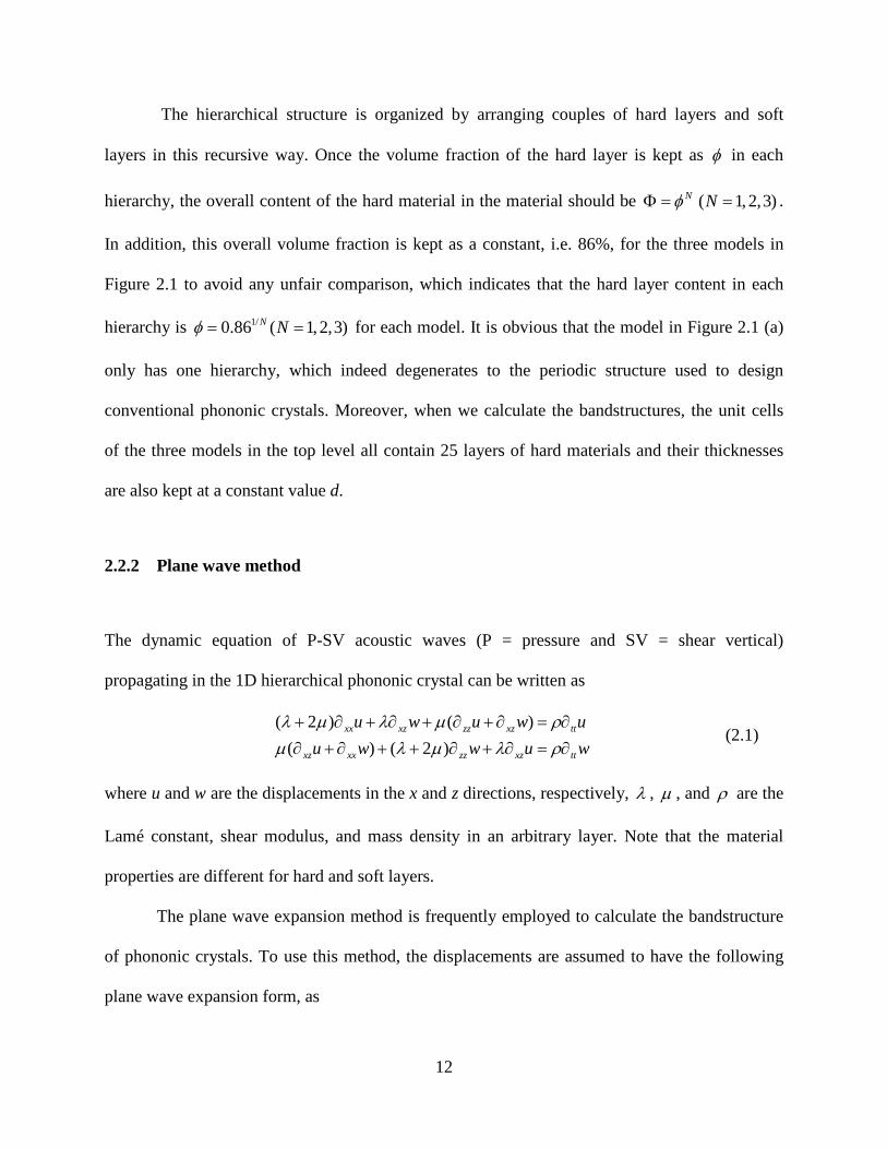
The hierarchical structure is organized by arranging couples of hard layers and soft
layers in this recursive way. Once the volume fraction of the hard layer is kept as φ in each
hierarchy, the overall content of the hard material in the material should be ( 1,2,3)N NφΦ = = .
In addition, this overall volume fraction is kept as a constant, i.e. 86%, for the three models in
Figure 2.1 to avoid any unfair comparison, which indicates that the hard layer content in each
hierarchy is 1/0.86 ( 1,2,3)N Nφ = = for each model. It is obvious that the model in Figure 2.1 (a)
only has one hierarchy, which indeed degenerates to the periodic structure used to design
conventional phononic crystals. Moreover, when we calculate the bandstructures, the unit cells
of the three models in the top level all contain 25 layers of hard materials and their thicknesses
are also kept at a constant value d.
2.2.2 Plane wave method
The dynamic equation of P-SV acoustic waves (P = pressure and SV = shear vertical)
propagating in the 1D hierarchical phononic crystal can be written as
( 2 ) ( )
( ) ( 2 )xx xz zz xz tt
xz xx zz xz tt
u w u w uu w w u w
λ µ λ µ ρµ λ µ λ ρ+ ∂ + ∂ + ∂ + ∂ = ∂∂ + ∂ + + ∂ + ∂ = ∂
(2.1)
where u and w are the displacements in the x and z directions, respectively, λ , µ , and ρ are the
Lamé constant, shear modulus, and mass density in an arbitrary layer. Note that the material
properties are different for hard and soft layers.
The plane wave expansion method is frequently employed to calculate the bandstructure
of phononic crystals. To use this method, the displacements are assumed to have the following
plane wave expansion form, as

13
i( ) i( )
i( ) i( )
e e
e e
x z m
x z m
k x t k G zm
m
k x t k G zm
m
u u
w w
ω
ω
− +
− +
=
=
∑
∑ (2.2)
where xk and zk are the wave vectors in x and z directions, ω is the angular frequency, and
2mG m dπ= ( 0, 1, 2,m = ± ± ) is the m-th lattice vector in the reciprocal space. In addition, the
material properties are also expanded in a Fourier series form, as
i[ , , ] [ , , ]e nG zn n n
nλ µ ρ λ µ ρ=∑ (2.3)
Thus, after substituting Eqs. (2.2) and (2.3) into Eq. (2.1), and collecting each wave mode n, the
governing equation of the n-th wave mode is
2 2
2
2 2 2
[ ( 2 ) ( ) ]
( ) ( )
( ) ( )
[ ( 2 )( ) ]
x n m n m n m z m mm
n m n m x z m m n m mm m
n m n m x z m mm
n m x n m n m z m m n m mm m
k k G u
k k G w u
k k G u
k k G w w
λ µ µ
λ µ ω ρ
λ µ
µ λ µ ω ρ
− − −
− − −
− −
− − − −
+ + +
+ + + =
+ +
+ + + + =
∑
∑ ∑
∑
∑ ∑
(2.4)
It should be pointed out that the sum of integer m or n in Eq. (2.4) is over all the reciprocal lattice
vectors. However, only the lowest 1000 modes are taken into account in this work, i.e.
, [ 1000,1000]m n∈ − , which will be exact enough for the first 100 phonon modes of interest here.
Eventually, Eq. (2.4) can be written in a matrix form, as
2ω=Ku Mu (2.5)
where K and M are the stiffness and mass matrices, and u is the displacement vector. The
frequencies can be readily obtained by solving the following eigenvalue problem, as
2det( ) 0ω− =K M (2.6)

14
where det( ) indicates the determinant of a matrix. Equations (2.4) and (2.6) are the general
equations determining the bandstructures of one-dimensional phononic crystals. However, those
equations can be simplified for 0xk = , in which case the longitudinal mode and transverse mode
can be decoupled. Accordingly, the equations in Eq. (2.4) become
2 2
2 2
( )
( 2 )( )
n m z m m n m mm m
n m n m z m m n m mm m
k G u u
k G w w
µ ω ρ
λ µ ω ρ
− −
− − −
+ =
+ + =
∑ ∑
∑ ∑ (2.7)
This simplification in Eq. (2.7) will reduce the computation time to a significant extent.
2.2.3 Phononic bandstructure
The material types of the hard layer and soft layer will not be specified in this theoretical study.
In addition, dimensionless material properties are chosen to simplify the numerical calculation.
In this case, the unit cell thickness in the top hierarchy is set as 1d = for the three models. As a
numerical example, the material properties are set as the following values:
110, 5, 1, 0.5
h s
h h s s
ρ ρλ µ λ µ
= == = = =
where the subscript h and s indicate the hard layer and soft layer, respectively. Note that the
elastic constants of the hard layer are ten times of that in the soft layer, which are already large
enough to form visible bandgaps in the phononic crystal.

15
Figure 2.2 Phononic band structure of hierarchical phononic crystals with different hierarchies. (a) One hierarchy
with d1 = 0.04 d; (b) Two hierarchies with d1 = 0.038 d; (c) Three hierarchies with d1 = 0.036 d. In this way, each
unit cell in the top level contains 25 layers of hard material for all the three models. The bandgaps are depicted in
red color, which indicates that more bandgaps can be generated once there are more hierarchies.
The bandgap characteristics of phononic crystals with different number of hierarchies are
shown in Figure 2.2, in which 0xk = and the dispersion curves are calculated in the irreducible
Brillouin zone ( [0, ]zk dπ= ). Thus, the phonon modes will include both longitudinal modes (P
wave) and transverse modes (SV wave). The frequency ω is plotted in logarithmic scale with
base 5 to show the bandgaps more clearly because the unit cell thickness in one hierarchy is
approximately five times of that in the lower hierarchy, i.e. 15 ( 2,3)i id d i−≈ = . As a result, the
frequency of the bandgap generated by each hierarchy obeys 1 5i iω ω −≈ , which is easier to show
in logarithmic scale. In addition, the thinnest unit cells in the three models of Figure 2.2 have
almost the same thickness d1 so that their phononic responses are comparable. Figure 2.2 (a)
shows the dispersion curves of a conventional periodic phononic crystal (N = 1) with unit cell
thickness as 0.04 d. Only one bandgap is observed near 5log 3.5ω = within the plotted frequency
range in Figure 2.2 (a). However, it is demonstrated that hierarchical structures can create more
(a) N=1 (b) N=2 (c) N=3

16
bandgaps at low frequency range. Those results are shown in Figure 2.2 (b) and (c), in which the
numbers of hierarchies are N = 2 and N = 3, respectively. Comparing Figure 2.2 (a) with Figure
2.2 (b), one more hierarchy generates at least three obvious bandgaps below the frequency
5log 3.2ω = in the crystal. In addition, the phononic crystal with three hierarchies (see Figure
2.3 (c)) has at least three additional bandgaps compared with the one of two hierarchies in Figure
2.2 (b). It is obvious from Figure 2.2 that the original bandgaps (bandgaps in the crystal with
lower hierarchy) still exist when one introduces an additional hierarchy, while more bandgaps
can be found at low frequency range. This is actually very useful because designing phononic
crystals with more and wider bandgaps is always an important goal for researchers. The reason
underlying this intriguing phenomenon is supposed to be the multilevel periodicity of the
hierarchical structure. This will be further confirmed and validated by the discussion on
bandgaps of simple periodic structures (N = 1) next.
Figure 2.3 Schematic illustration of the bandgap formation mechanism in phononic crystal with two hierarchies.
The bandgaps of the hierarchical phononic crystal in (d) include contributions from the two hierarchies in (b) and (c)
separately.
(a)
(b)
(c)
(d)

17
The bandgap formation mechanism in a hierarchical phononic crystal is illustrated in
Figure 2.3. It is hypothesized that different hierarchies in the crystal will perform almost
independently. Therefore, each hierarchy can create some bandgaps in the phononic crystal, and
the whole hierarchical structure can integrate all those bandgaps together. For example, the
hierarchical crystal shown in Figure 2.3 has a bandgap close to 5log 3.5ω = , which is formed by
the first hierarchy in Figure 2.3 (b), while some additional bandgaps at lower frequency range are
induced by the second hierarchy in Figure 2.3 (c). This mechanism can also be generalized and
extended to hierarchical phononic crystals with more hierarchies. Thus it is expected that more
hierarchies will create more bandgaps, as what has been shown in Figure 2.2. To prove the
mentioned hypothesis, let us consider the bandgaps of phononic crystals with only one hierarchy
but different unit cell thickness. The results of those models are shown in Figure 2.4, in which
(a), (b), and (c) actually show the contributions to the bandgaps from the first, second, and third
hierarchies in Figure 2.1, respectively. The bandstructures in Figure 2.4 are already well
understood by researchers. It shows that rescaling the unit cell thickness will not change the
property of the band structure so much, but the dispersion curves will rescale accordingly. By
comparing Figure 2.2 and Figure 2.4, it can be found that Figure 2.2 (a) and Figure 2.4 (a) are
actually the same. However, the bandgaps in Figure 2.2 (b) are approximately the superposition
of bandgaps in Figure 2.4 (a) and (b), that is, bandgaps contributed by the first and second
hierarchy. Similarly, the bandgaps of phononic crystal with three hierarchies (see Figure 2.2 (c))
can integrate the bandgaps of all three models in Figure 2.4, which further validates our
hypothesis. By comparing Figure 2.4 with Figure 2.2, it is obvious that more hierarchies will
generate more wide bandgaps, which will enhance the wave reflectance of the phononic crystal.
Thus, it is concluded that bandgaps of the hierarchical phononic crystals contain the contribution
18
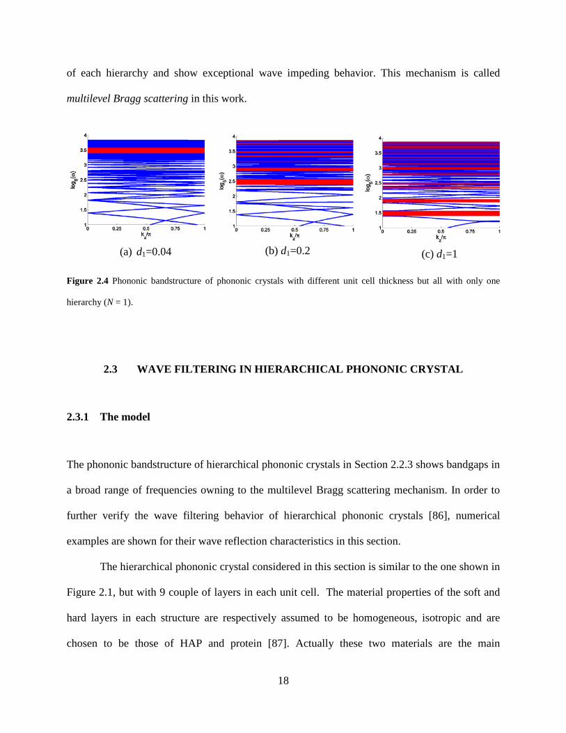
of each hierarchy and show exceptional wave impeding behavior. This mechanism is called
multilevel Bragg scattering in this work.
Figure 2.4 Phononic bandstructure of phononic crystals with different unit cell thickness but all with only one
hierarchy (N = 1).
2.3 WAVE FILTERING IN HIERARCHICAL PHONONIC CRYSTAL
2.3.1 The model
The phononic bandstructure of hierarchical phononic crystals in Section 2.2.3 shows bandgaps in
a broad range of frequencies owning to the multilevel Bragg scattering mechanism. In order to
further verify the wave filtering behavior of hierarchical phononic crystals [86], numerical
examples are shown for their wave reflection characteristics in this section.
The hierarchical phononic crystal considered in this section is similar to the one shown in
Figure 2.1, but with 9 couple of layers in each unit cell. The material properties of the soft and
hard layers in each structure are respectively assumed to be homogeneous, isotropic and are
chosen to be those of HAP and protein [87]. Actually these two materials are the main
(a) d1=0.04 (b) d1=0.2 (c) d1=1

19
constituents in many hierarchical biological materials including bone, enamel, etc. The overall
volume fraction of the hard material in each of the hierarchical models ( 1, 2,3N = ) is taken as
0.86Φ = . This requires that the content of hard layer in each hierarchy set to be 1 Nφ = Φ in each
model; for example, the volume fraction of hard layer will be 0.95 at each level n for the N = 3
model and 0.93 for the N = 2 model. In turn, the thickness of the unit cell at each hierarchy can
be connected by a scaling law as 1n nd d m f− = for any 1n > .
Table 2.1 Material properties of the constituent materials
λ (GPa) µ (GPa) ρ (kg/m3)
HAP 37 31.5 3190
Protein 1.2 0.3 1400
Water 2.36 0 1050
The governing equation for the elastic P-SV (P-pressure and SV-shear vertical) wave
propagation in a multilayered material can be expressed as [88, 89]:
( ) ( ) ( )z z z zω∂ =b A b (2.8)
where T( ) [ ]z x zz xzz u u σ σ=b is the displacement-stress vector as a function of depth z with u
being the displacement, σ the stress, ω the angular frequency, and A a matrix related to the
depth-dependent density and elastic properties of the constituent materials [69, 90, 91] shown in
Table 2.1. The subscripts x and z denote the respective axes parallel and perpendicular to the
layers in the structure (see Figure 2.1). Through the transfer matrix formulation, the solution to
Eq. (2.8) can be shown to be ( ) exp[i ] (0)z zω=b Α b . However, the transfer matrix formulation
may introduce some numerical instability at high frequencies since the solution procedure

20
involves subtraction of exponential growing terms. The method proposed by Kennett [88] is
adopted to stabilize the calculation, where reflection and transmission matrices are introduced to
eliminate the exponential growing terms analytically. To this end, the dynamic response of the
whole material can be obtained once the boundary value (0)b due to the incident wave is
prescribed. Thereafter, the reflectance of the hierarchical material is computed as the ratio of the
energy flux, i.e., 0.5Re[i ( )]z zz x xzu uω σ σ+ [89], of the incident wave to that of the reflected wave
at the left end (see Figure 2.1). If the reflectance is equal to unity in a certain range of
frequencies, the incident wave will be totally reflected, and hence a bandgap can be identified.
2.3.2 Wave reflection in hierarchical phononic crystal
The wave reflectance of each multilayered hierarchical structure with different levels of
hierarchy is shown in Figure 2.5, in which the reflectance spectra under P wave incident at an
angle 0θ = in water are illustrated. The unit cell thickness at the finest hierarchy level n = 1 in
each model is taken to be d1 = 0.1 μm. In addition, the three hierarchical structures are of equal
total thickness (100 μm) to avoid any unfair comparison. Figure 2.5 (a) shows the reflectance of
the periodic structure (i.e. N = 1), where the lowest-frequency bandgap can be identified to be
10 114 10 ~2 10× × rad/s. These characteristics show that this periodic structure is poor at impeding
waves at frequencies 104 10< × rad/s. In contrast, more bandgaps can be created in lower
frequency range by simply adding more hierarchy levels to this periodic structure. This is
demonstrated in Figure 2.5 (b) and (c), which show that approximately 5 and 12 more bandgaps
are created at frequencies 104 10< × rad/s for the respective multilayered structures with N = 2
and N = 3 levels of hierarchy when compared with the periodic structure (Figure 2.5 (a)). Note

21
that the lowest-frequency bandgap is formed at 9~ 5 10× rad/s and 8~ 6 10× rad/s as shown in
Figure 2.5 (b) and (c), respectively. Thus it can be concluded that adding one more level of
hierarchy with longer period can create more bandgaps at nearly one order of magnitude lower in
frequency. Further, it can also be observed that having more levels of hierarchy will also increase
the reflectance in higher frequency range (i.e. 112 10ω > × rad/s). The overall behavior observed is
remarkable because hierarchical structure provides a way to impede wave propagation in a much
broader range of frequencies, which enhances the wave filtering ability of phononic crystals. The
origin of this effect should be due to the multilevel Bragg scattering of the hierarchical structured
models constructed above and will be further explored in the discussion of bandgaps of periodic
structures next.
Figure 2.5 Reflectance spectra of hierarchical materials with N levels of hierarchy.

22
Figure 2.6 Reflectance spectra of periodic and stacked structures. (a)-(c) Single periodic structures consisting of ten
unit cells with d1 = 0.1 μm, d1 = 0.95 μm, and d1 = 8.98 μm, respectively. (d) Reflectance spectrum of a multilayered
structure constructed by stacking the three models of (a)-(c) in series.
Here, each level of hierarchy in the previous hierarchical structures is modeled
independently as a periodic structure, and the wave reflectance will be compared to those of the
hierarchical structures. Each of the three periodic structures has 10 unit cells, whose respective
thickness 1d is the same as that at level n = 1, 2, and 3 in the three previous hierarchical
structures. The resulting reflectance spectra under normal P wave incident are plotted in Figure
2.6 (a)-(c), which are consistent with the scaling law mentioned above [67]. By comparing
Figure 2.5 with Figure 2.6 (a)-(c), the hierarchical structures generally have more wide bandgaps
than the periodic structures, which enables the strong reflection of incident waves in a wide
range of frequencies. In fact, the bandgaps of the hierarchical structures with N = 2 and 3 levels

23
of hierarchy (Figure 2.5) seem to have superimposed, to a large extent, the widest bandgaps of
the periodic structures when the same periodicity is embedded in the hierarchical structures. For
example, the wave reflectance of the hierarchical structure with N = 3 (Figure 2.5 (c)) shows
bandgaps created by all three periodic structures shown in Figure 2.6 (a)-(c). Therefore, this
multilayered structure with three hierarchy levels has much wider bandgaps at the high
frequencies than the response of periodic structure shown in Figure 2.6 (c). Equally importantly,
the overall bandwidth covered by closely adjacent bandgaps of the two hierarchical structures is
thus approximately one and two orders of magnitude larger than that of the periodic structures in
this case. Further confirmation can be provided by computing the reflectance spectrum of a
structure constructed by stacking the three periodic models of Figure 2.6 (a)-(c) in series. This
structure contains a total of 30 unit cells and can superimpose all the widest bandgaps in Figure
2.6 (a)-(c) perfectly. It can be seen that the hierarchical structure in Figure 2.5 (c) has similar
broadband wave filtering effect with this stacked structure in Figure 2.6 (d), although some tiny
pass bands are observed in the former, e.g., see the one at 8 96 10 ~ 2 10× × rad/s. Actually it is
possible to tune the three periodicities such that the bandgaps are perfectly back-to-back, or even
overlapping, by employing the stacking design of Figure 2.6 (d). However, it is unlikely for the
hierarchical structure to get rid of the tiny pass bands. Surely, the bandgaps of hierarchical
structures are not just simple superposition of the ones generated by periodic structures
corresponding to each level. In reality, adding one more level of hierarchy introduces periodic
defects to the periodicity at the lower hierarchy level. These defects do not affect the bandgaps
so much despite introducing some phonon modes in the tiny pass bands. However, the
disadvantage is outweighed by the advantages of this bioinspired hierarchical structure over
simple stacked periodic structures in series: 1) it is much more compact in thickness and uniform

24
in response due to the inherent multiscale periodicity; 2) it is cheaper to assemble because only
hard building blocks of the same size are needed; 3) it also endows the phononic material with
other exceptional mechanical behaviors such as enhanced strength and toughness. Therefore,
hierarchical structure is promising for phononic crystal design [92].
Figure 2.7 Contour plot of the reflectance of multilayered hierarchical models with N = 3 levels of hierarchy.
The incident P wave has been set normal to the material surface in the models employed
to generate the response in Figure 2.5 and Figure 2.6. Hence the reflection response of the
hierarchical material with N = 3 levels of hierarchy will be examined for waves at incident angles
of 0 ~80 , as shown in the contour plot in Figure 2.7. One can observe from Figure 2.7 that a
wide range of bandgaps still exist when the incidence angle θ becomes larger. In particular, the
hierarchical material has a very wide bandgap when ~ 70θ . This contour plot demonstrates that
the hierarchical structure is also effective in filtering waves from different directions at a wide
range of frequencies.

25
2.4 SUMMARY
In summary, it has been demonstrated through a simple multilayered model that the hierarchical
structure observed in the bone-like biological materials can be designed as phononic crystals
exhibiting bandgaps in much broader frequency range than those with single periodicity. The
incident waves of a wide frequency range could be totally reflected in these bioinspired
hierarchical structures to dissipate energy, which partially answers the first question raised in
Section 1.3. This remarkable feature is attributed to the intrinsic multilevel periodicity of
hierarchical structures, which gives rise to the multilevel Bragg scattering phenomenon. More
specifically, the periodicity in each hierarchy level creates bandgaps in certain ranges of
frequency, and the whole hierarchical structure superimposes the bandgaps generated in each
hierarchy together, which shows strong filtering effect to the incident waves. It is also found that
the introduction of an additional level of hierarchy would not affect the original bandgaps much,
although sometimes a small pass band can occur and split the original bandgap. The conceptual
design and mechanism presented in this chapter can be readily adopted to enhance wave filtering
and reflection of periodic structures by turning them into hierarchical structures.

26
3.0 HIERARCHICAL STAGGERED COMPOSITES WITH HIGHLY ENHANCED
DAMPING
3.1 INTRODUCTION
The damping composites have wide applications in engineering. For example, they could serve
as cushion layers to protect objects from dynamic attack or disturbance, control the vibration of
load-bearing structures as a damping component, and design structures or parts with intrinsic
energy dissipation behaviors. Even though the damping is a fundamental and ubiquitous
behavior of all solid materials [93], only a few of them reach the standard of engineering
damping application. The design of high-performance wave or vibration absorbing structural
components requires materials having high viscosity and moderate to high stiffness. The
damping performance of materials [93] is characterized by their complex modulus iE E E∗ ′ ′′= + ,
with the real part E′ (storage modulus) and imaginary part E′′ (loss modulus) being proportional
to the storage energy and dissipated energy in the materials, respectively, and their ratio
tan E Eδ ′′ ′= known as the loss tangent (or viscosity) of materials. The loss modulus
tanE E δ′′ ′= , a direct indicator of the energy dissipation, is also designated as the figure of merit
of damping materials. In general, most materials show poor damping performance because they
do not usually exhibit both high stiffness E′ and high viscosity tanδ simultaneously [15, 94].

27
For example, soft polymers usually have high viscosity ( tanδ = 0.1 ~ 1) but stiff materials like
metals normally exhibit much lower viscosity ( tanδ < 0.001) at room temperature [93].
Several methods have been proposed in the literature to design better performing
damping materials, like introducing piezoelectric or magnetostrictive phases [95, 96], employing
phase transitions [97, 98], synthesizing nanocomposites [99, 100], and adding negative-stiffness
phases [101, 102]. Nevertheless, one cannot underestimate the role of biological materials,
especially those with high specific loss modulus, in inspiring and stimulating the design of
materials with high energy dissipation [5]. For example, dissipative bio-inspired scaffolds have
been recently synthesized by replicating the pore structure of cancellous bones [103]. In addition,
some theoretical and numerical works have shown that the bone- and nacre-like structure could
be utilized to design phononic crystals with highly enhanced wave reflection/absorption
performance [86, 104, 105] and to attenuate wave propagation at nanoscale [106]. A comparison
study by Lakes [15, 93] showed that most materials have a damping figure of merit lower than
0.6 GPa, while cortical bone exhibits a comparatively high damping for a relatively stiff
material. For example, its stiffness is normally 12~20 GPa [8-10] while damping loss factor is
0.01~0.1 [16-19] over a range of frequencies. This implies that there is possibility to design
composites exhibiting high stiffness and large damping loss factor simultaneously by mimicking
the bone structure. It would be of great significance to develop such composites with highly
enhanced energy dissipation for engineering applications. Hence, the objective of this chapter
includes three aspects: (i) Design and model staggered composites with better damping
performance; (ii) Manufacture and test staggered polymer composites with enhanced energy
dissipation; (iii) Explore the effect of structural hierarchy on the damping of staggered materials.

28
3.2 STAGGERED COMPOSITE DESIGN
The two-dimensional (2D) staggered composite shown in Figure 3.1 mimics the microstructure
of bone and nacre [4], which has drawn much attention and extensive investigation. For example,
this model has been successfully used to explain the stiffness and toughness enhancement
mechanism in 2D staggered composites [23, 25, 26, 107-110]. In a 2D staggered composite, the
hard prisms (or platelets) are dispersed in the soft matrix in a staggered manner (Figure 3.1 (b)).
The length and thickness of the prism is l and h , respectively, which also define its aspect ratio
as l hη = with η≫1. The thickness of the soft matrix layer is ch and the distance between two
neighbor prism tips is cl ( cl ≪ l ). The loading-transfer characteristic in the 2D staggered
composite is quite unique. The uniaxial loading along the longitudinal direction of prisms is
mainly sustained by the shear deformation of the soft matrix within the shear region (Figure 3.1
(b)) between two parallel prisms [23], even though the soft matrix in the tension region (Figure
3.1 (b)) has a minor effect [111]. The force balance of the prism is illustrated in Figure 3.1 (c),
where cτ is the shear stress in the shear region and cσ is the tensile stress in the tension region.
Note that cτ is not necessarily constant along the prism surface, especially when the aspect ratio
η is large. Since the loading-transfer is mainly induced by the shear region, we define the
effective shear length of a prism as s cl l l= − and the corresponding aspect ratio as /s sl hη = .
Note that the difference between η and sη is only significant when the aspect ratio η is small.

29
Figure 3.1 Biomimetic design of 2D staggered composites from the bone structure. (a) The mineralized fibril
structure of cortical bone [4]. The mineral platelets are arranged in a layer-wise staggered manner. (b) Arrangement
of the hard prisms in the designed composite. (c) Force balance diagram for an individual prism.
Three-dimensional (3D) staggered composites are designed as a substitute for the 2D
model since the 2D model suffers from low loading-transfer ability. In reality, the staggered
microstructure is akin to 3D rather than 2D in natural materials such as bone and nacre [77, 112,
113]. Compared with the 2D design, 3D staggered composites have more topological features to
be designed and optimized, providing a greater possibility to leverage the loading-transfer
ability. Therefore, two different kinds of 3D staggered composites are designed, which have
square (Figure 3.2 (a)) and hexagonal (Figure 3.2 (d)) shaped prisms, respectively. The structure
of 3D staggered composites is more complex than the 2D case. For both of the two types of 3D
staggered composites, shown in Figure 3.2, the prisms are distributed so that one prism’s tip
locates in the middle of adjacent prisms in the longitudinal direction. The prism’s length,
thickness, and aspect ratio are also designated as l , h , and η , respectively. Other parameters,
like sl , sη , ch , and cl , can also be defined in accordance with the 2D case. The detailed
arrangement of the prisms in 3D staggered composites is illustrated in Figure 3.2 (b) and (e),
which show the cellular structure of their transverse cross sections. The lattice points are

30
indicated by black dots and defined by two lattice vectors 1a and 2a . Similar to a crystal
structure [114], the structure of a staggered composite is determined once its motif, the repeated
unit cell resting at each lattice point, is prescribed. The representative motifs of 3D staggered
composites are enclosed and highlighted by dotted closed circles in Figure 3.2 (b) and (e). Each
motif contains two arrays of prisms, which arrange in a staggered manner and are differentiated
by solid lines and dashed lines in Figure 3.2. The lattice points of the staggered composites can
be obtained via translation operations based on the lattice vectors, which are defined as
1 2[1 1], [1 1]= =a a , and 1 2[ 3 0], [0 1]= =a a for square and hexagonal cases, respectively.
The edge length a of the prism is derived from the geometric condition, where a h= and
3a h= for square and hexagonal prism, respectively. Therefore, once the volume fraction of
the hard phase is set as φ , the soft layer thickness is determined by
1
0.5
( 1) for 2D case( 1) for square or hexagonal prismc
hh
hφφ
−
−
−=
− (3.1)
It is found from Eq. (3.1) that the soft layer thicknesses of the two 3D staggered composites
(with square and hexagonal prisms) are equal when the volume fraction φ and prism thickness
h are fixed.
The loading-transfer characteristics are different for the two composites presented in
Figure 3.2. As shown in Figure 3.2 (b), all of the four nearest neighbors of a square prism have
different arrangement compared to itself, which induces shear stress cτ on all of its four lateral
surfaces (Figure 3.2 (c)) once a uniaxial loading is applied to the composite. In contrast, the
hexagonal prism (Figure 3.2 (d) and (e)) has a different feature, that is, only four lateral surfaces
out of six are subjected to shear stress loading, as illustrated in Figure 3.2 (f). Thus, the shear
region can be formed all around a square prism but only partially around a hexagonal prism. It is

31
shown that both 3D designs have more effective loading-transfer ability than the 2D one.
Additionally, similar to the 2D staggered composite, the tensile stress cσ is also be induced by
the tension region, which has a minor effect on the deformation of a prism but should not be
neglected when the aspect ratio η of the prism is not large enough.
Figure 3.2 Schematic illustration of 3D staggered composites with (a)-(c) square prisms and (d)-(f) hexagonal
prisms. (a) and (d) show the prism arrangement in each composite. (b) and (e) show the lattice structure of the
transverse cross section of each composite. Lattice points are indicated by black dots. The motif is enclosed by a
dotted closed circle, which contains two columns of prisms arranged in a staggered manner and being indicated by
solid and dash lines, respectively. (c) and (f) illustrate the force balance diagram of a prism in the corresponding
composite.

32
3.3 THEORETICAL MODELING
The complex modulus of staggered composites can be derived from the correspondence principle
of linear viscoelasticity [93, 115]. Namely, the dynamic property of viscoelastic materials
follows the same mathematical form as the elastic case by simply replacing all real elastic
constants with complex values. Therefore, the elastic properties are derived first.
3.3.1 A unified shear-lag model
A unified shear-lag model is presented to predict the overall elastic property of all three
staggered composites. As shown in Figure 3.3, the motif structure of each 3D composite is
further reduced to a simple model (shaded area in Figure 3.3) containing two reduced prisms
bonded by a soft layer. The mechanical response of the reduced model is equivalent to the whole
composite due to the lattice symmetry conditions. In fact, the reduced model in Figure 3.3 is just
a quarter of the Wigner-Seitz cell of the lattice structure for the two composites with square
(Figure 3.2 (b)) and hexagonal (Figure 3.2 (e)) prisms. The cross sectional area A of each
reduced prism is
12
214
23 38
for 2D plane stressfor square prism
for hexagonal prism
ahA a
a
=
(3.2)
Note that the area A is also able to be expressed as a function of h only.
33
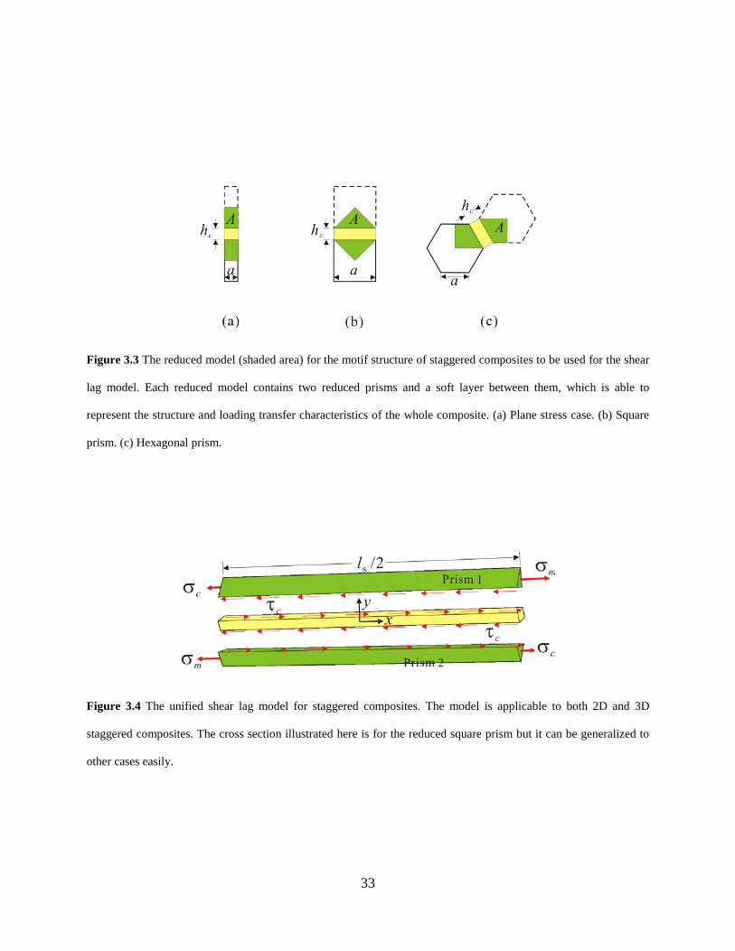
Figure 3.3 The reduced model (shaded area) for the motif structure of staggered composites to be used for the shear
lag model. Each reduced model contains two reduced prisms and a soft layer between them, which is able to
represent the structure and loading transfer characteristics of the whole composite. (a) Plane stress case. (b) Square
prism. (c) Hexagonal prism.
Figure 3.4 The unified shear lag model for staggered composites. The model is applicable to both 2D and 3D
staggered composites. The cross section illustrated here is for the reduced square prism but it can be generalized to
other cases easily.

34
The shear lag model is illustrated in Figure 3.4, which is composed of two reduced
prisms and a soft layer between them. The maximum tensile stress mσ occurs in the middle of
each prism due to the symmetry condition. Thereby, only a half of the reduced prism needs to be
considered in the shear lag model. A local coordinate system is established at the center of the
soft layer with x denoting the longitudinal direction of the prism and hence 4 4s sl x l− ≤ ≤ . In
Figure 3.4, prism 1 is subjected to tensile stress loading cσ and mσ on its two ends, where cσ is
the tensile stress induced by the tension region. In contrast, prism 2 is subjected to the same
tensile stress loading but on opposite ends. Suppose the displacement field in the prism is ju and
jv along the x and y direction, respectively, with the subscript ( 1, 2)j j = indicating the prism
number. An essential assumption of the shear lag model is that ( )j ju u x= and 0jv = . Thus the
prisms are in uniaxial tension and the misfit displacement 1 2u u− will induce shear deformation
in the soft layer. Therefore, the shear strain cγ in the shear region of the soft layer is
1 2c
c
u uh
γ −= (3.3)
In turn, the shear strain cγ asserts shear stress loading to the two prisms, as
1 2( )
c c c
c
c
u uh
τ µ γµ
=
= − (3.4)
where cµ is the shear modulus of the soft matrix.
The unknown displacements 1u and 2u will be solved from the equilibrium equation of
the prisms, as [116]
1
2
x c
x c
A aA a
σ τσ τ
∂ =∂ = −
(3.5)

35
where A is shown in Eq. (3.2). Given that the tension strain is j x juε = ∂ in the two prisms, the
corresponding tensile stress is
j m j
m x j
EE u
σ ε=
= ∂ (3.6)
where mE is the elastic modulus of the prism. Alternatively, the equilibrium equations in Eq.
(3.5) can be further written in a displacement form by employing Eq. (3.6), as
2
1 1 22
2
2 1 22
( ) 02
( ) 02
xxs
xxs
ku u ulku u ul
∂ − − =
∂ + − = (3.7)
where k is a dimensionless parameter related to the prism shape and material properties, as
22 c s
m c
alkE Ahµ
= (3.8)
It will be shown later that k is a crucial geometrical parameter reflecting the loading-transfer
ability of a staggered composite.
The boundary conditions of the two prisms are set as
1 4
1 4
2 4
2 4
0
s
s
s
s
cx l
mx l
x l
cx l
u
σ σ
σ σ
σ σ
=−
=
=−
=
=
=
=
=
(3.9)

36
Figure 3.5 Schematic illustration of the deformation in the tension region of the soft matrix for a stretched 2D
staggered composite. The initial boundary of the tension region is a rectangle, whereas the deformed boundary is an
octagon. The tension deformation in the tension region can be generalized to 3D cases similarly.
Up to now, the tensile stress cσ is still unknown, which is induced by the deformation of the
tension region. It is seen from Figure 3.5 that the rectangular tension region deforms into an
octagon shape in the 2D staggered composite. Actually the deformation of the tension region is
similar in 3D staggered composites. The tensile strain of the tension region between the two
prism tips can be derived from the kinematic relation in Figure 3.5, as
4
2s
cc c x l
c
hl
ε γ=
= (3.10)
Thus the average tensile stress cσ exerted on the prism tip is estimated to be
c cc
c εσφ
= (3.11)
where the term φ in the denominator is introduced to account for the tension effect of the soft
material on the left and right sides of the tension region. The result of Eq. (3.11) has been proved

37
to be valid even for 3D staggered composites. The term cc is the tensile stiffness [117] of the
soft material, as
2 for plane stress
1(1 ) for other cases
(1 )(1 2 )
c
cc
c c
c c
E
cEν
νν ν
−= − + −
(3.12)
where cE and cν are the elastic modulus and Poisson's ratio of the soft matrix and
2 (1 )c c cE µ ν= + . After substituting Eqs. (3.3) and (3.10) into Eq. (3.11), the tensile stress cσ is
expressed in a displacement form, as
1 2 4
2 ( )s
cc x l
c
c u ul
σφ =
= − (3.13)
By substituting Eq. (3.13) into the boundary conditions in Eq. (3.9), the displacement
field ( 1, 2)ju j = is able to be solved from Eq. (3.7), as
cosh( )2
4 cosh( 4)2
1 ( )2 4 tanh( 4)
j sc s
m c
c
m c s
kx lc lE l km s
j c km E l l
xlu xE k
ζφ
φ
σ + + + = + + +
(3.14)
where
1 for 11 for 2j
jj
ζ=
= − = (3.15)
The tensile stress in the prism is determined by Eqs. (3.6) and (3.14), as
sinh( )2cosh( 4)
212 tanh( 4)
j sc
m c s
c
m c s
k kx lcE l l km
j c kE l l k
ζφ
φ
σσ + = + +
(3.16)
In addition, the shear stress distribution in the shear region of the soft matrix is obtained from
Eqs. (3.4) and (3.14), as

38
cosh( )cosh( 4)
2 tanh( 4)
s
c
m c s
kx lkc m
c c km c E l lE h kφ
µ στ
= + (3.17)
Equation (3.17) indicates that cτ is not always constant along the prism. Only in the case that
4k ≪1 can cτ be assumed to be constant.
3.3.2 Elastic modulus of staggered composites
The overall elastic modulus of the staggered composites is derived based on the proposed shear
lag model above. Bear in mind that the left end of prism 2 in Figure 3.4 is fixed. Hence, the
overall strain of the staggered composite is
1 4
2sx l
s
u
lε == (3.18)
On the other hand, the average stress in the composite is [23]
( )m cσ σ σ φ= + (3.19)
The overall elastic modulus E σ ε= of the staggered composite can be obtained from
Eqs. (3.18) and (3.19) with given displacement field in Eq. (3.14) and stress distribution in Eq.
(3.16). It is finally found that
4 4
1 1 1tanh( )s
c
l k km c mlE E c Eφ φ
= ++
(3.20)
where the first term on the right hand side shows the contribution from the prism and the second
term represents the effect of the soft matrix. The simple form of Eq. (3.20) has a very strong
physical implication, that is, the hard prism and soft matrix behave like a pair of springs in series
while the soft matrix itself is just like connecting its tension region and shear region in parallel.

39
Note that Eq. (3.20) is a unified formula for both 2D and 3D staggered composites. The
topology feature of different shapes of prisms is reflected in the parameter k defined by Eq.
(3.8). It is seen from Eq. (3.20) that the parameter k is an effective stiffness indicator of the
shear region of the soft matrix. A larger k value indicates that the shear region is more effective
in loading transfer. Equation (3.8) implies that, to increase k , one may either increase the edge
length a of the prism or reduce the soft layer thickness ch , which can be achieved by changing
the shapes of prisms. Specifically, k has the following form for different staggered composites,
as
1
0.5
0.5
( 1)
( 1)
43 ( 1)
2 for plane stress
2 2 for square prism
for hexagonal prism
c
m
c
m
c
m
s E
s E
s E
k
µφ
µφ
µφ
η
η
η
−
−
−
−
−
−
=
(3.21)
It is found from Eq. (3.21) that the loading transfer ability of these staggered composites follows
the sequence square > hexagonal > 2D. Therefore, the aspect ratio sη of the prism can be
reduced if 3D designs are used instead of the 2D one.
The elastic modulus formula Eq. (3.20) derived from the shear lag model can be
simplified when k is small. This derives from the fact that tanh( 4) 4k k≈ when 4k ≪1. In
this case, the simplified elastic modulus is
2
1 1 116m c s c mE E c l l E kφ φ
≈ ++
(3.22)
After substituting the k values in Eq. (3.21) to Eq. (3.22) and employing Eq. (3.12), the elastic
modulus for the staggered composites can be written in a unified form, as
2
1 1 ( )
m c s
fE E
φφ αµ φη
≈ + (3.23)

40
where
1
0.5
0.5
4( 1) for plane stress( ) 2( 1) for square prism
3( 1) for hexagonal prismf
φφ φ
φ
−
−
−
−= − −
(3.24)
and α is a correction factor introduced to account for the tension region effect, which is
8(1 )
4(1 )(1 2 )
6(1 )(1 2 )
1 for plane stress
1 for square prism
1 for hexagonal prism
c
c s c
c c
c s c
c c
c s c
hl
hl
hl
ν η φ
νν η φ
νν η φ
α−
−−
−−
+= ++
(3.25)
Note that the effect of the tension region would be excluded once 1α = . Equation (3.23)
indicates that the effect of the tension region can be incorporated by simply multiplying the shear
modulus cµ of the soft matrix by a factor α . In addition, this correction factor 1α → when the
shear aspect ratio sη increases, which indicates that the tension region effect is only significant
when sη is small. It has been proven [111] that this correction factor can enhance the accuracy of
the model a lot and should not be neglected.
The simplified elastic modulus formula in Eq. (3.23) is quite convenient to use and
predicts satisfactory results in most cases, even though the one in Eq. (3.20) is more accurate in
theory. For practical usage, one is strongly advised to check the criterion 4k ≪1 first with k
given by Eq. (3.21) to determine whether the shear-lag model or simplified model should be
adopted.

41
3.3.3 Complex modulus of staggered composites
Given that the elastic moduli of staggered composites have been derived in Section 3.3.2, their
complex moduli can be readily obtained by replacing the elastic modulus mE of the hard phase
and shear modulus cµ of the soft matrix with the corresponding complex constants,
i imm m m mE E e E Eδ∗ ∗ ′ ′′= = + and i ic
c c c ce δµ µ µ µ∗ ∗ ′ ′′= = + , respectively. As a result, the parameter k
in Eqs. (3.8) and (3.21) and stiffness cc in Eq. (3.12) can also be transformed to their complex
counterpart as k∗ and cc∗ by replacing the material constants. Note that the Poisson's ratio mν
and cν are assumed to be real and unchanged in both the static or dynamic cases. Finally, the
complex modulus of staggered composites is obtained directly from Eq. (3.20) according to the
correspondence principle, as
4 4
1 1 1tanh( )s
c
l k km c mlE E c Eφ φ ∗ ∗∗ ∗ ∗ ∗= +
+ (3.26)
The exact storage modulus E′ , loss modulus E′′ , and loss tangent tanδ of staggered
composites can all be obtained from Eq. (3.26) by separating the real and imaginary parts of E∗ .
In addition, the optimal damping situation can also be evaluated numerically by solving for the
optimal aspect ratio ˆsη .
Some approximated analytical formulae of E∗ , E′ , E′′ , and tanδ for staggered
composites are shown. These are derived based on the simplified model presented in Section
3.3.2. In this case, the complex modulus corresponding to Eq. (3.23) can be written as
2
1 1 ( )
m c s
fE E
φφ αµ φη∗ ∗ ∗≈ + (3.27)
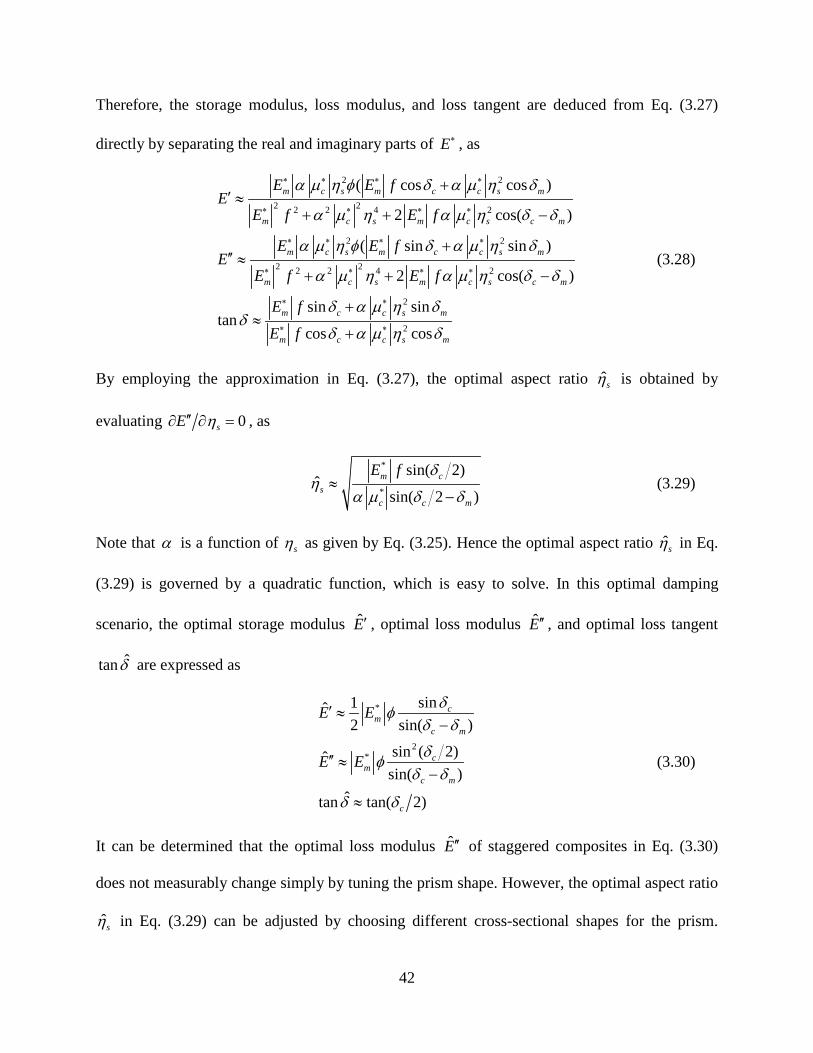
42
Therefore, the storage modulus, loss modulus, and loss tangent are deduced from Eq. (3.27)
directly by separating the real and imaginary parts of E∗ , as
2 2
2 22 2 4 2
2 2
2 22 2 4 2
2
2
( cos cos )
2 cos( )
( sin sin )
2 cos( )
sin sintan
cos c
m c s m c c s m
m c s m c s c m
m c s m c c s m
m c s m c s c m
m c c s m
m c c s
E E fE
E f E f
E E fE
E f E f
E f
E f
α µ η φ δ α µ η δ
α µ η α µ η δ δ
α µ η φ δ α µ η δ
α µ η α µ η δ δ
δ α µ η δδ
δ α µ η
∗ ∗ ∗ ∗
∗ ∗ ∗ ∗
∗ ∗ ∗ ∗
∗ ∗ ∗ ∗
∗ ∗
∗ ∗
+′ ≈
+ + −
+′′ ≈
+ + −
+≈
+ os mδ
(3.28)
By employing the approximation in Eq. (3.27), the optimal aspect ratio ˆsη is obtained by
evaluating 0sE η′′∂ ∂ = , as
*
*
sin( 2)ˆ
sin( 2 )m c
sc c m
E f δη
α µ δ δ≈
− (3.29)
Note that α is a function of sη as given by Eq. (3.25). Hence the optimal aspect ratio ˆsη in Eq.
(3.29) is governed by a quadratic function, which is easy to solve. In this optimal damping
scenario, the optimal storage modulus E′ , optimal loss modulus E′′ , and optimal loss tangent
ˆtanδ are expressed as
*
2*
sin1ˆ2 sin( )
sin ( 2)ˆsin( )
ˆtan tan( 2)
cm
c m
cm
c m
c
E E
E E
δφδ δ
δφδ δ
δ δ
′ ≈−
′′ ≈−
≈
(3.30)
It can be determined that the optimal loss modulus E′′ of staggered composites in Eq. (3.30)
does not measurably change simply by tuning the prism shape. However, the optimal aspect ratio
ˆsη in Eq. (3.29) can be adjusted by choosing different cross-sectional shapes for the prism.
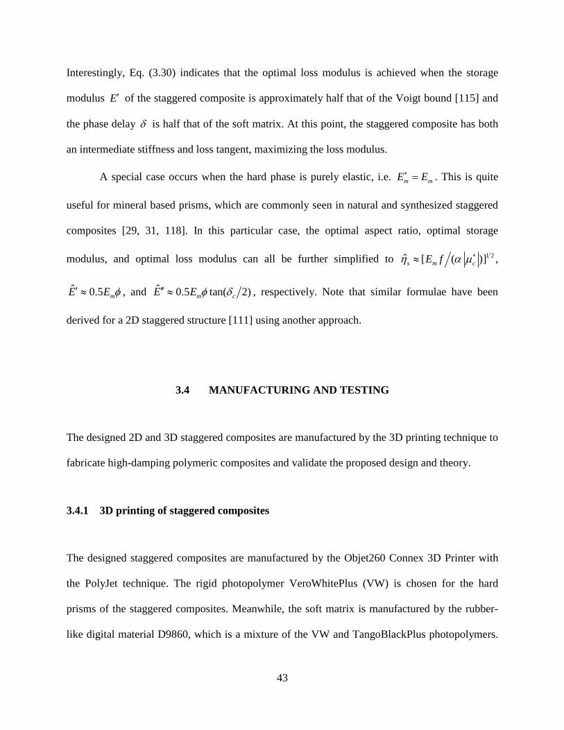
43
Interestingly, Eq. (3.30) indicates that the optimal loss modulus is achieved when the storage
modulus E′ of the staggered composite is approximately half that of the Voigt bound [115] and
the phase delay δ is half that of the soft matrix. At this point, the staggered composite has both
an intermediate stiffness and loss tangent, maximizing the loss modulus.
A special case occurs when the hard phase is purely elastic, i.e. m mE E∗ = . This is quite
useful for mineral based prisms, which are commonly seen in natural and synthesized staggered
composites [29, 31, 118]. In this particular case, the optimal aspect ratio, optimal storage
modulus, and optimal loss modulus can all be further simplified to 1 2ˆ [ ( )]s m cE fη α µ∗≈ ,
ˆ 0.5 mE E φ′ ≈ , and ˆ 0.5 tan( 2)m cE E φ δ′′ ≈ , respectively. Note that similar formulae have been
derived for a 2D staggered structure [111] using another approach.
3.4 MANUFACTURING AND TESTING
The designed 2D and 3D staggered composites are manufactured by the 3D printing technique to
fabricate high-damping polymeric composites and validate the proposed design and theory.
3.4.1 3D printing of staggered composites
The designed staggered composites are manufactured by the Objet260 Connex 3D Printer with
the PolyJet technique. The rigid photopolymer VeroWhitePlus (VW) is chosen for the hard
prisms of the staggered composites. Meanwhile, the soft matrix is manufactured by the rubber-
like digital material D9860, which is a mixture of the VW and TangoBlackPlus photopolymers.

44
Specifically, the VW is mainly synthesized from acrylic monomers, isobornyl acrylate, and
acrylic oligomers; while the TangoBlackPlus is mainly synthesized from acrylic oligomers and
isobornyl acrylate (see PolyJet Photopolymers Material Safety Datasheets, Stratasys Ltd.). Note
that only one UV lamp is used to cure the photopolymers in the 3D printer according to its
default setting. Figure 3.6 (a)-(c) show three examples of the manufactured staggered
composites. The thickness of each prism is 1 mmh = and the volume fraction of the prisms is
0.5φ = . The associated cross sections of the 3D staggered composites show regular arrangement
of the prisms, which are consistent to the designed pattern shown in Figure 3.1 and Figure 3.2.
The manufactured staggered composites used for dynamic testing are shown in Figure 3.6
(e)-(g). Rectangular cross sections are used for these specimens in order to be in compliance with
the ASTM standards for dynamic testing of plastics (i.e. ASTM D4065 and ASTM D5026).
Different from the staggered composite samples in Figure 3.6 (a)-(c), two 25 mm long grip ends
are printed using VW for each of the testing specimen, which will prevent damage to the D9860
material or staggered composites induced by the grips of the testing apparatus. The volume
fraction of the VW prisms is 0.5φ = for all the staggered composites printed. In addition, the
thickness of each prism is 1 mmh = while the aspect ratio η varies from 6 to 18. The thickness
of the soft matrix in the tension region is kept as cl h= so it is obvious that 1sη η= − for these
composite samples. All testing specimens are manufactured with their thickness direction normal
to each printing layer and longitudinal axis along the printing head scanning direction. The
specimens are kept on the building tray inside the printer chamber for two hours after printing in
order to cool and further stabilize. The surfaces of the specimens are then cleaned by water jet to
remove the support resin (SUP705). After removing the support resin, the specimens are dried in
room condition for one hour and stored in sealed bags for ten hours before testing.

45
Figure 3.6 Staggered polymer composites manufactured by the PolyJet 3D printing technique by using two
polymers of VW (in white color) and D9860 (in black color). The three kinds of staggered composites (ϕ = 0.5, η =
12) are shown in (a) 2D composite, (b) 3D composite with square prisms, and (c) 3D composite with hexagonal
prisms, all accompanied with their cross sections. (d)-(g) show the 3D printed specimens for mechanical testing. All
specimens contain two VW grip ends to prevent damaging induced by the grips of the load frame. (d) Testing
specimens of VW (left) and D9860 (right). (e), (f), and (g) show a full set of 2D staggered composites, 3D staggered
composites with square prisms, and 3D staggered composites with hexagonal prisms, respectively. Note that the
seven specimens in (e)-(g) have a volume fraction of ϕ = 0.5 and aspect ratios as η = 6, 9, 10, 12, 14, 15, and 18,
respectively (from left to right in each image).

46
3.4.2 Static and dynamic testing
All tests are performed on an MTS880 system at 20 C . The static tensile tests of VW and
D9860 specimens are performed at a strain rate of 10.156 minε −= and 10.178 minε −= ,
respectively. The dynamic mechanical behaviors are tested by applying a cyclical tensile strain
loading (at 1 Hz) on specimens and measuring the stress response. A pretension strain of
0 1%ε = and 0 11.6%ε = , respectively, is applied to the VW and D9860 specimens before
applying the cyclic strain loading. The pretension strain is necessary to prevent any compression
induced buckling of the specimens under the cyclic loading condition (ASTM D4065 and ASTM
D5026). Note that the overall strain should not exceed the viscoelastic regime of the materials.
For example, the cyclic tensile strain amplitudes are about 0.5% and 2.5% for the VW and
D9860 specimens, respectively (see Figure 3.7 (b) and (d)).
Figure 3.7 shows some representative testing results of the VW and D9860. For the static
tensile responses, the VW has an elastic limit of 2%ε ≈ while that for D9860 can be up to
45%ε ≈ . Some visible cracks would occur in the D9860 specimens once the tensile strain
45%ε > . The dynamic stress-strain relations of VW and D9860 are shown in Figure 3.7 (b) and
(d), respectively. The loss tangent of D9860 is nearly ten times larger than that of the VW.
However, the energy dissipation capacity of D9860 is much less than the VW since it is too soft.
Note that the loss modulus of D9860 is only 6% of the VW, which is proportional to the
dissipated energy. These two kinds of photopolymers have comparably higher viscosity ( tanδ )
compared with other kinds of polymers at the room temperature [5].

47
Figure 3.7 Typical mechanical responses of the VeroWhitePlus (VW) photopolymer and the digital material D9860.
(a) Static test of a VW specimen. (b) Cyclic dynamic test of a VW specimen at 1 Hz and 20 ◦C. (c) Static test of a
D9860 specimen. (d) Cyclic dynamic test of a D9860 specimen at 1 Hz and 20 ◦C. The dissipated energy is equal to
the area enclosed by the hysteresis circle in (b) and (d).
Table 3.1 Material properties of VeroWhitePlus (VW) and the digital material D9860. Dynamic material properties
are measured at 1 Hz and 20 ◦C.
E (MPa) ν E′ (MPa) E′′ (MPa) tanδ ρ (Kg/m3)
VW 1859 ± 11 0.33 2043 ± 80 215 ± 2 0.1~0.11 1160 ± 10
D9860 2.1~2.2 0.45 12.1 ± 0.8 12.7 ± 0.3 1.05 ± 0.04 1145 ± 15

48
The mechanical behaviors of the constituent materials used to fabricate the composites
are introduced first. Table 3.1 shows the static and dynamic material properties of VW and
D9860. It can be seen that the VW is a rigid plastic while the D9860 behaves like soft viscous
rubber. The storage modulus of VW is a bit higher than its elastic modulus since the latter is
measured at a quite low strain rate. The loss tangent tanδ of VW is comparable to that of
PMMA (at 1 Hz, room temperature). In contrast, the digital material D9860 is quite viscous with
a loss tangent of tan 1.05δ = , a very high value for elastomers at room temperature. In addition,
the storage modulus and loss modulus of D9860 are much higher than its elastic modulus.
Figure 3.8 Storage moduli, loss moduli, and loss tangent of staggered composites obtained from theory and
experiments. (a) 2D staggered composite. (b) 3D staggered composite with squared prisms. (c) 3D staggered
composite with hexagonal prisms. All dynamic tests are performed at 1 Hz and the room temperature.
The manufactured staggered polymer composites are tested under cyclic dynamic loading
to validate the theory established above. The full set of the test specimens is shown in Figure 3.6
(e)-(g). All specimens are tested at 20 C with a frequency of 1 Hz. A pretension strain of ∼1%
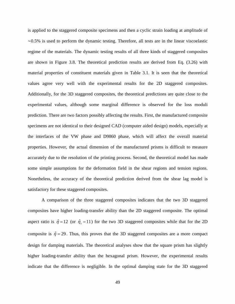
49
is applied to the staggered composite specimens and then a cyclic strain loading at amplitude of
∼0.5% is used to perform the dynamic testing. Therefore, all tests are in the linear viscoelastic
regime of the materials. The dynamic testing results of all three kinds of staggered composites
are shown in Figure 3.8. The theoretical prediction results are derived from Eq. (3.26) with
material properties of constituent materials given in Table 3.1. It is seen that the theoretical
values agree very well with the experimental results for the 2D staggered composites.
Additionally, for the 3D staggered composites, the theoretical predictions are quite close to the
experimental values, although some marginal difference is observed for the loss moduli
prediction. There are two factors possibly affecting the results. First, the manufactured composite
specimens are not identical to their designed CAD (computer aided design) models, especially at
the interfaces of the VW phase and D9860 phase, which will affect the overall material
properties. However, the actual dimension of the manufactured prisms is difficult to measure
accurately due to the resolution of the printing process. Second, the theoretical model has made
some simple assumptions for the deformation field in the shear regions and tension regions.
Nonetheless, the accuracy of the theoretical prediction derived from the shear lag model is
satisfactory for these staggered composites.
A comparison of the three staggered composites indicates that the two 3D staggered
composites have higher loading-transfer ability than the 2D staggered composite. The optimal
aspect ratio is ˆ 12η = (or ˆ 11sη = ) for the two 3D staggered composites while that for the 2D
composite is ˆ 29η = . Thus, this proves that the 3D staggered composites are a more compact
design for damping materials. The theoretical analyses show that the square prism has slightly
higher loading-transfer ability than the hexagonal prism. However, the experimental results
indicate that the difference is negligible. In the optimal damping state for the 3D staggered

50
composites, the storage modulus, loss modulus, and loss tangent are measured to be
520 MPaE′ = , 209 MPaE′′ = , and tan 0.4δ = , which are quite close to the optimal values
predicted by Eq. (3.30), as 577 MPaE′ = , 247 MPaE′′ = , and tan 0.43δ = , respectively. In
conclusion, these dynamic test results for staggered composite specimens validate the designed
model and proposed theory above.
Figure 3.9 Schematic illustration of the damping enhancement mechanism in staggered composites. The
deformation mechanism changes from soft-matrix-dominate to hard-phase-dominate at the optimal damping state
( ˆs sη η= ). Both the storage modulus and loss tangent have monotonic relations with respect to the aspect ratio sη
while the loss modulus has a peak.
3.4.3 Damping enhancement mechanism
Why does the loss modulus have an optimal value in staggered composites, and what is the
mechanism? The answer is illustrated schematically in Figure 3.9. The storage modulus E′ of
the staggered composites is bounded by the Voigt bound, while its loss tangent tanδ is bounded

51
by that of the constituent materials. Consequently, the storage modulus E′ increases from cE′ to
mEφ while the loss tangent tanδ decreases from tan cδ to tan mδ when sη increases from 0 to
∞. Thus the loss modulus E′′ , i.e. the product of E′ and tanδ , might have an optimum E′′ at
certain point ˆs sη η= depending on the varying rate of the storage modulus and loss tangent. For
the current problem, it is found that the loss modulus depends on the competition between the
deformation in the hard phase and soft matrix. In the case that ˆs sη η< , the deformation of
staggered composites is dominated by that of the soft matrix. The large shear deformation in the
shear region of the soft matrix will increase the energy dissipation in the whole composite.
However, once ˆs sη η> , large tension deformation occurs in the hard phase, which dominates the
contribution from the soft matrix. Therefore, even though the overall storage modulus E′ of the
composite still increases, tanδ and E′′ decrease because the hard phase has low (or even none)
energy loss. Therefore, the optimal state is achieved when the storage modulus contributions
from the hard phase and soft matrix are equal. In this situation, the soft matrix provides the most
efficient energy dissipation and both phases contribute to the overall storage modulus of the
composite. It is the unique deformation mechanism transition from soft-matrix-dominant to hard-
phase-dominant that induces the significant damping enhancement in staggered composites [5,
111]. The storage modulus, loss modulus, and loss tangent at this optimal state can be found in
Eq. (3.30). In addition, the optimal aspect ratio ˆsη is affected by the type of staggered
composites. In theory, a staggered composite with higher loading-transfer ability would exhibit
smaller ˆsη . Hence the 3D staggered composites with comparatively high volume fraction are
recommended to design and manufacture better-performance damping materials.

52
3.5 HIERARCHICAL STAGGERED COMPOSITES
3.5.1 Effect of structural hierarchy
It has been reported that the stiffness, toughness, strength, and wave filtering of the material may
be further enhanced by introducing more hierarchies [1, 23, 78, 86, 108, 119-121]. Would more
hierarchies also affect the damping property of the hierarchical staggered materials? To answer
this question, a 2D hierarchical staggered composite (see Figure 3.10) is studied, which contains
elastic hard phases and a viscoelastic soft matrix. Note that the designed material has a self-
similar structure in each hierarchy and form a total number of N hierarchies. Hence, the overall
volume fraction of the hard phase is NφΦ = given that φ is the volume fraction of the platelets
in each hierarchy.
Figure 3.10 Schematic illustration of a hierarchical staggered structure with three hierarchies.
The complex modulus of this 2D hierarchical staggered composite can be derived from
Eq. (3.27) in a recursive way, as
2 21
1 1 4(1 )
n n c sE Eφ
φ αµ φ η∗ ∗ ∗−
−= + (3.31)
Level 3
Level 2
Level 1
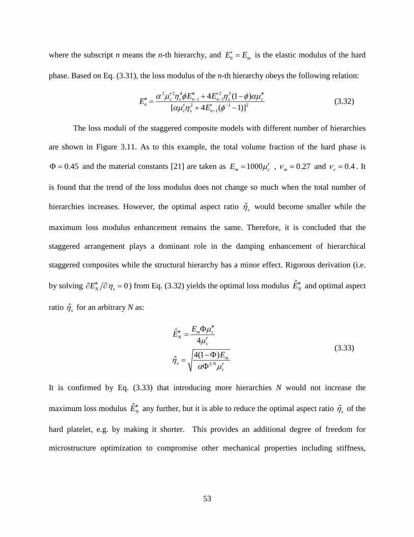
53
where the subscript n means the n-th hierarchy, and 0 mE E∗ = is the elastic modulus of the hard
phase. Based on Eq. (3.31), the loss modulus of the n-th hierarchy obeys the following relation:
2 4 22 2
1 11 2
12
4 (1 )[ 4 ( 1)]c s n c
nc ns
n sE EEE
α µ φ φ αµη ηα ηµ φ
− −−
−
′ ′′ ′ ′′+ −′′ =′ ′+ −
(3.32)
The loss moduli of the staggered composite models with different number of hierarchies
are shown in Figure 3.11. As to this example, the total volume fraction of the hard phase is
0.45Φ = and the material constants [21] are taken as 1000m cE µ′= , 0.27mν = and 0.4cν = . It
is found that the trend of the loss modulus does not change so much when the total number of
hierarchies increases. However, the optimal aspect ratio ˆsη would become smaller while the
maximum loss modulus enhancement remains the same. Therefore, it is concluded that the
staggered arrangement plays a dominant role in the damping enhancement of hierarchical
staggered composites while the structural hierarchy has a minor effect. Rigorous derivation (i.e.
by solving 0N sE η′′∂ ∂ = ) from Eq. (3.32) yields the optimal loss modulus ˆNE′′ and optimal aspect
ratio ˆsη for an arbitrary N as:
1
ˆ4
4(1 )ˆ
mN
c
m
c
s Nc
EE
E
µ
η
µ
α µ
′Φ′′ =′
−Φ=
′Φ
′
(3.33)
It is confirmed by Eq. (3.33) that introducing more hierarchies N would not increase the
maximum loss modulus ˆNE′′ any further, but it is able to reduce the optimal aspect ratio ˆsη of the
hard platelet, e.g. by making it shorter. This provides an additional degree of freedom for
microstructure optimization to compromise other mechanical properties including stiffness,

54
strength, toughness, etc. Normally these properties cannot achieve the optimal state
simultaneously and a multiple-objective optimization is needed.
Figure 3.11 Loss modulus enhancement of staggered structures with different number of hierarchies.
3.5.2 Comparison with other composites
According to the analysis and discussion above, we can readily derive an upper bound for the
loss modulus enhancement in hierarchical staggered composites, which is actually an alternative
expression to the first equation in Eq. (3.33), as ˆ 0.25 tanN m cE E δ′′ = Φ . This staggered structure
actually achieves a high stiffness and a large loss factor simultaneously compared to many other
composites shown in Figure 3.12. It is a common belief that an increase in stiffness of a material
will oftentimes reduce its damping behavior [15]. For example, the Voigt composite and Hashin-
Shtrikman (H-S) composite (upper bound) have high stiffness but low damping [93]. In contrast,
the Reuss composite and H-S composite (lower bound) may show significant damping property,
but their stiffness is commonly very low except the case with extremely high content of hard
phase [93]. However, the staggered structure can overcome this difficulty. It can be seen in

55
Figure 3.12 that the loss modulus of the hierarchical staggered composite can be tens of times
larger than the H-S lower bound in most cases and it does not require very large hard phase
content. Alternatively, there is a tradeoff between the hard phase content and its aspect ratio. If
there is less hard phase, one can still achieve high damping performance by increasing the aspect
ratio of hard platelets. This behavior is attributed to the unique microstructure as well as the
anisotropy of the staggered structure. This is not ubiquitous because the material’s stiffness can
be enhanced drastically by introducing anisotropy but its damping property normally does not
follow the same way [15]. However, the staggered composite is an exception, which can be
optimized to achieve damping performance much better than many other structures. Another
advantage of the hierarchical staggered composite is its high toughness and strength [21, 22,
108]. In contrast, it was found that the soft material is subjected to large stress in the Reuss and
H-S composites, which are very weak and cannot be used as structural materials [93].
Nevertheless, the hierarchical staggered structure provides a way to design damping materials
that incorporate high damping, stiffness, toughness, and strength.
Figure 3.12 Comparison of loss modulus enhancement of several composites.
56
3.6 SUMMARY
In summary, the staggered composite design inspired from the bone structure has been proven to
exhibit highly enhanced damping behavior. This anomalous phenomenon originates from the
unique deformation characteristics in the staggered composites. Namely, the large shear
deformation of the soft viscous matrix will result in high energy dissipation, while the hard phase
endows the composite with high stiffness simultaneously. The optimal damping state is attained
when the hard phase and soft phase have equal contribution to the overall storage modulus of the
composites. According to this mechanism, three different kinds of staggered polymer composites
are designed, tested, and compared. It is found that the 3D composites with square or hexagonal
prisms have much higher loading-transfer ability than the 2D design. A much smaller aspect
ratio of the hard phase is required to achieve the same storage modulus and loss modulus in the
3D design compared with the 2D one. A theoretical study on the effect of structural hierarchy
indicates that the total number of hierarchies would not affect the optimal loss modulus of the
staggered composites. However, the optimal aspect ratio of the platelet could be reduced if more
hierarchies are introduced. In addition, this staggered composite can exhibit a much larger loss
modulus than the Voigt, Reuss and H-S composites, regardless of the volume fraction of the hard
phase. The present findings provide insight into the energy dissipation mechanism in bone-like
structures and offer a useful way to design novel composites with excellent damping property.

57
4.0 SYMMETRY, ANISOTROPY, AND SYMMETRY BREAKING OF CELLULAR
STRUCTURES
4.1 INTRODUCTION
Cellular structures are composed of porous unit cells organized in a periodic or random pattern
[24]. The periodic cellular structures are similar to single crystals since both of them have
periodic lattice points and repetitive motif [122]. However, the cellular structures are much more
complex than single crystals. For instance, the unit cell size of cellular structures ranges from
nanometers to millimeters. In addition, the material distribution in the unit cell of cellular
structures could be designed in favor of the required performance. Therefore, cellular structures
have drawn much attention by researchers from fabrication to application. Particularly, the
design and fabrication of cellular structures have benefited from the modern fabrication
techniques. For example, the widely used techniques include material removal method (e.g.
etching), 3D printing [51, 55, 123], etc. Up to now, cellular structures of different material types
have been fabricated at all scales including nano-, micro-, and macro-scale.
Similar to crystals, the long-range physical properties of cellular structures must be
compatible with their point group symmetry according to the Neumann’s law [124]. The
relations between point group symmetry and physical properties of crystals have been studied
extensively and outlined in [124, 125]. The physical properties (e.g. elastic, thermal, dielectric,

58
etc.) are usually represented by different ranks of tensors, which are invariant or form-invariant
under symmetry transformations of the material point group. Therefore, the long-range physical
properties of cellular structures could be determined qualitatively once their symmetry is known.
However, the point group symmetry of cellular structures is more complex than that of single
crystals. Note that the unit cell of a cellular structure may have complex topology and material
heterogeneity that cannot be easily determined through visualization. Thus, there is a strong
demand for a theoretical framework to analyze and determine the point group symmetry of
cellular structure systematically.
Another interesting problem is the deformation induced symmetry breaking [56, 126-
128], which arises in cellular structures (or single crystals as well) once a strain field is imposed.
This phenomenon is important in at least two applications. First, the symmetry breaking of
cellular structures may lead to changes of their physical properties, which opens opportunities to
tune/control the physical performance and design functional materials. For example, deformation
induced acoustic, optical, and thermal property changes in materials are reported in the literature
[127, 129-131]. Secondly, the symmetry evolution is also important for the constitutive modeling
of cellular structures because the symmetry property changes must be considered when modeling
the material property evolution during deformation [132, 133]. Therefore, the symmetry
evolution of cellular structures after deformation is discussed in this chapter with an emphasis on
the symmetry breaking at small strain cases.
The main aim of this chapter is to study the symmetry characteristics of cellular
structures. To achieve this goal, a theoretical framework is proposed to describe and determine
the point group symmetry of cellular structures [61] with several examples discussed. Thereafter,
the symmetry breaking of deformed cellular structures is introduced.

59
4.2 POINT GROUP SYMMETRY THEORY
The scientific notations used in Chapters 4 and 5 are summarized. We use calligraphy letters for
sets (e.g. ,A B ), R for the real number set, N for the natural number set, 3R for the 3D
Euclidean space, lowercase Greek letters for scalars (e.g. ,α β ), lowercase bold-face letters for
vectors (e.g. ,a b ), uppercase bold-face letters for second-order tensors (e.g. ,A B ), uppercase
blackboard letters for fourth-order tensors (e.g. , ), and uppercase bold-face script letters for
point groups (e.g. ,A B ). The inner products are defined as ij j iA b=Ab e and ij jk i kA B= ⊗AB e e ,
where ie is the basis vector, ⊗ is the dyadic product, and Einstein’s summation rule applies. In
addition, the Hermann-Mauguin notation [122] is adopted to represent the material point groups.
4.2.1 3D material point groups
There are totally 32 crystal point groups and 7 continuous point groups for 3D materials [122].
Each crystal point group contains a finite number of symmetry transformations, whereas the
continuous point groups are non-compact. In order to describe these symmetry transformations, a
Cartesian coordinate system is established, which has three orthogonal axes 1e , 2e , and 3e . Each
crystal class has three preferred lattice vectors 1a , 2a , and 3a according to the convention of
crystallography [122]. The default material orientations are introduced first, which follow the
notations used in [134, 135]. (i) Triclinic lattices can be arbitrarily oriented. (ii) The lattice vector
1a is parallel to the axis 1e for monoclinic lattices. (iii) For the rhombic, tetragonal, and cubic
systems, 1a , 2a , and 3a are parallel to the axes 1e , 2e , and 3e , respectively. (iv) For the

60
hexagonal system, 1a and 3a are parallel to the axes 1e and 3e , respectively. Note that the
trigonal crystal system is classified into the hexagonal system here [134]. The detailed symmetry
transformations of 32 crystal point groups are listed in [134, 135].
Besides the 32 crystal point groups, there are two isotropy groups ( m∞∞ and ∞∞ ) and
five transverse isotropy groups (∞ , m∞ , m∞ , 2∞ , and mm∞ ) in 3D [122, 124]. The group
m∞∞ is equal to the 3D orthogonal group (3)O , while the group ∞∞ is equal to the 3D proper
orthogonal group (3)+O . On the other hand, all transverse isotropy groups have a preferred
rotation axis along 3e . The rotation transformation is represented by a continuous function, as
cos sin 0sin cos 00 0 1
θ
θ θθ θ
= −
M (4.1)
where 0 2πθ≤ ≤ . All the symmetry transformations of transversely isotropic groups [134] can
be generated by θM and the diagonal matrices 1 diag( 1,1,1)= −R , 3 diag(1,1, 1)= −R , and
2 diag( 1,1, 1)= − −D . All 3D continuous point groups are listed in Table 4.1.
Table 4.1 Symmetry transformations of continuous point groups in 3D
Class Symmetry Transformations
m∞∞ (3)O
∞∞ (3)+O
∞ θM
m∞ θM , 1R , 1θM R
m∞ θM , 3R , 3θM R
2∞ θM , 2D , 2θM D
mm∞ θM , 1R , 3R , 2D , 1θM R , 3θM R , 2θM D

61
4.2.2 Point group theory of cellular structures
An example is illustrated in Figure 4.1 to show the multilevel structural feature of cellular
structures and the complexity of their symmetry. Different from single crystals, cellular
structures have symmetry and translation order at multiple structural levels, and each level may
have different symmetry properties. For example, Figure 4.1 (a) shows a cubic cellular structure
at level 1 (the coarsest scale) with its constituent material exhibiting a hexagonal lattice at level 2
(finer scale). Overall, the symmetry of cellular structures has three unique properties compared
with that of single crystals [61]. (i) The point group symmetry of cellular structures may not be
the same at different levels. (ii) The lattice orientations may be distinct across different levels,
even if they belong to the same point group. (iii) The material components of the cellular
structure unit cell could have different materials, orientations, and symmetries. It is thus clear
that the multilevel structural feature and complex unit cell topology lead to great difficulty in
determining the overall symmetry of cellular structures by visualization alone. To address this
issue, a theoretical framework is established to characterize and determine the point group
symmetry of cellular structures in a systematic manner. Without loss of generality, we focus on
cellular structures with two structural levels since they are commonly seen. The proposed theory
could be easily applied to cellular structures with three levels or more [86, 136] using a
hierarchical approach.

62
Figure 4.1 An Octet cellular structure composed of a material with hexagonal lattice in level 2. All the ligaments
have the same material type and orientation.
The point group of a two-level cellular structure is determined by examining its
symmetry at both level 1 and level 2. Thus, the symmetry of the topology, material type, material
orientation, and local material point group should be evaluated when the reference configuration
3⊂B R is mapped to the transformed configuration 3′ ⊂B R (see Figure 4.2), where B and
′B are sets containing all material points and the prime symbol indicates quantities or fields
after a symmetry transformation. Hence, a material point ∈X B will be mapped to the point
′ ′∈X B after the transformation [137]. The symmetry of cellular structures is more complicated
than the classical point group theory of single crystals, which only considers the symmetry of the
atom location and species in a unit cell. Therefore, we will divide the symmetries of cellular
structures into two categories: Topology symmetry and material symmetry.
(1) Topology symmetry. This includes the symmetries of the geometry and material type,
which are determined at level 1. Herein the material type merely means the material name and
phase (e.g. copper with face-centered cubic lattice), regardless of the material orientation. The
material type field is characterized by a scalar function 3( ) :ϕ X R N since the material type
Level 2 Level 1 Cellular structure

63
of each material point could be labeled as a natural number. Thereafter, the topology point group
{ }= TT of the cellular structure is defined as
: { ( ) ( ) ( ), }d ϕ ϕ= ∈ = ∀ ∈T TX X X BT O | (4.2)
where ( )dO represents the orthogonal group in 3R . Equation (4.2) is derived from the fact that
( )ϕ ϕ ϕ′ ′≡ =X when the map ′ =X X TX does not change the material type field.
Alternatively, the topology symmetry of the cellular structure is preserved once the material type
field ( )ϕ X is invariant under a symmetry transformation.
(2) Material symmetry. This includes the symmetry properties of the local material
orientations and local point groups at level 2 of a cellular structure. Generally, not all operations
in the topology point group T guarantee the material symmetry at level 2. Hence, by denoting
the overall point group of the cellular structure as { }= GG , it is obvious that G must be a
subgroup of T , as
≤G T (4.3)
A concept of material point group field is introduced first, i.e. ( )XM , which is a function
mapping an arbitrary material point ∀ ∈X B to its corresponding local material point group.
Note that ( )XM could even have different orders for different material points. As shown in
Figure 4.2, the material point group field ( )XM should be form-invariant under symmetry
transformations, as
T( ) ( ) ,′ ′≡ = ∀ ∈X G X G X BM M M (4.4)
where the superscript ‘T’ indicates the transpose operation and T T: { | }= ∀ ∈G G GMG MM M .
Therefore, the point group G is defined based on Eqs. (4.3) and (4.4), as
T: { ( ) ( ) ,= ∈ = ∀ ∈G GX G X G X BG T|M M } (4.5)
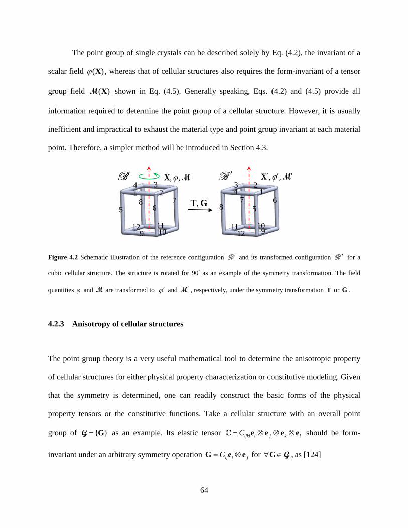
64
The point group of single crystals can be described solely by Eq. (4.2), the invariant of a
scalar field ( )ϕ X , whereas that of cellular structures also requires the form-invariant of a tensor
group field ( )XM shown in Eq. (4.5). Generally speaking, Eqs. (4.2) and (4.5) provide all
information required to determine the point group of a cellular structure. However, it is usually
inefficient and impractical to exhaust the material type and point group invariant at each material
point. Therefore, a simpler method will be introduced in Section 4.3.
Figure 4.2 Schematic illustration of the reference configuration B and its transformed configuration ′B for a
cubic cellular structure. The structure is rotated for 90◦ as an example of the symmetry transformation. The field
quantities ϕ and M are transformed to ϕ′ and ′M , respectively, under the symmetry transformation T or G .
4.2.3 Anisotropy of cellular structures
The point group theory is a very useful mathematical tool to determine the anisotropic property
of cellular structures for either physical property characterization or constitutive modeling. Given
that the symmetry is determined, one can readily construct the basic forms of the physical
property tensors or the constitutive functions. Take a cellular structure with an overall point
group of { }= GG as an example. Its elastic tensor ijkl i j k lC= ⊗ ⊗ ⊗e e e e should be form-
invariant under an arbitrary symmetry operation ij i jG= ⊗G e e for ∀ ∈G G , as [124]
,T G
, ,ϕX M , ,ϕ′ ′ ′X M
1 2 3 4
5 6 7 8
9 10 11 12
1 2 3
5 7
9 10
4 6
8 11
12
B ′B

65
ijkl ia jb kc ld abcdC G G G G C= (4.6)
For example, the elastic tensor of the five cubic point groups (23, 3m , 432, 43m , and 3m m ) has
the following form [125] in the Voigt notation, as
11 12 12
11 12
11
44
44
44
0 0 00 0 00 0 0
0 0sym. 0
c c cc c
cc
cc
=
(4.7)
However, the elastic tensor of the tetragonal point groups ( 4 mmm , 4mm , 422, and 42m ) is
11 12 13
11 13
33
44
44
66
0 0 00 0 00 0 0
0 0sym. 0
c c cc c
cc
cc
=
(4.8)
In addition, if one considers the yield behavior of cellular structures, the yield function should at
least satisfy the following objective form [137], as
T2PK 2PK( ) ( ),f f= ∀ ∈σ Gσ G G G (4.9)
where 2PKσ is the second Piola-Kirchhoff stress tensor. In fact, the yield function is usually
expressed in terms of the invariants of the stress tensor and the structural tensor which
characterizes the material point group symmetry.
The topology point group T of some typical cellular structures is shown in Table 4.2.
Note that the overall point group G also depends on the material distribution and orientation in
level 2.
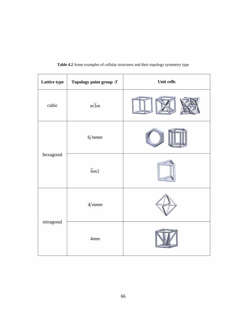
66
Table 4.2 Some examples of cellular structures and their topology symmetry type
Lattice type Topology point group T Unit cells
cubic 3m m
hexagonal
6 mmm
6 2m
tetragonal
4 mmm
4mm

67
4.3 DETERMINATION OF THE POINT GROUP OF CELLULAR STRUCTURES
4.3.1 Overview of the method
A practical method is proposed to determine the point group of the cellular structures. The
cellular structure unit cell is divided into Mn material components, each with the same material
type and orientation, and then their symmetry properties are compared. For example, the unit cell
in Figure 4.2 has twelve material components ( 12Mn = ), which are numbered in sequence.
Denote the symmetry orders of the point groups G and T as Gn and Tn , respectively, which
satisfy G Tn n≤ according to Eq. (4.3). Thus, under the l-th topology symmetry transformation
( )l Tl n∈ ≤T T at level 1, a material component is transformed to the position of another one,
forming a pair of material components whose local material symmetries at level 2 should be
examined. Consequently, a total of l Mn n= (or 2l Mn n= for some cases) pairs of material
components will be formed under the l-th transformation l ∈T T . Finally, the overall point group
G will be determined after evaluating the material symmetries of all 1
Tnll
n=∑ pairs of material
components for every topology symmetry transformation in T .
4.3.2 Symmetry of a pair of material components
As illustrated in Figure 4.3, the material symmetry of two material components lkB and lk′B is
studied first, which are the k-th pair ( )lk n≤ of material components related to the topology
symmetry transformation l ∈T T , i.e. the configuration transformation is l′ =X X T X for

68
lk∀ ∈X B . For the sake of convenience, two local Cartesian coordinate systems lkx and lk′x are
established for the material components lkB and lk′B , respectively, according to the convention
of crystallography for lattice orientations. By this means, the material point groups of lkB and
lk′B have a unified form as { }lk lk= MM in their own local coordinate systems, which results in
great simplification for the analysis. Note that the material point groups of lkB and lk′B can also
be represented in the global coordinate system X , which is correlated to the local coordinate
systems by lk lk=x Q X and lk lk′ ′=x Q X , where lkQ and lk′Q are orthogonal transformation
matrices. Therefore, in the global coordinate system, the material point groups lkM and lk′M of
the two material components lkB and lk′B are expressed as
T
T
lk lk lk lk
lk lk lk lk
=
′ ′ ′=
Q Q
Q Q
M M
M M (4.10)
Figure 4.3 Schematic illustration of the material symmetry transformation of a pair of material components in a
cellular structure unit cell.
X
lkB lk′B
lkx lk′x
lkQ lk′Q
lTlkM lk′M

69
Further, it is obtained from Eq. (4.10) that the relation between lkM and lk′M is
T Tlk lk lk lk lk lk′ ′ ′= Q Q Q QM M (4.11)
Equation (4.11) implies that lkM and lk′M are conjugate [138].
The material symmetry of lkB and lk′B is examined under the corresponding topology
symmetry transformation l ∈T T . Based on Eq. (4.5), the material symmetry of lkB and lk′B
requires that Tl lk l lk′=T TM M . In addition, the point group lk′M does not change under a symmetry
transformation of its own members, i.e. Tlk lk lk lk′ ′ ′ ′= M MM M . Finally, it is obtained that the
material symmetry condition of the two material components is
T
T
T T T , for
l lk l lk
lk lk lk
lk lk lk lk lk lk lk lk lk
′=
′ ′ ′=
′ ′= ∀ ∈
T TM MQ Q M M Q Q M
M M
M
M M
(4.12)
where the last equality is derived by using Eq. (4.11). Thus it is found from Eq. (4.12) that the
material symmetry of the k-th pair of material components can only be conserved when
Tl lk lk lk′∈T Q Q M (4.13)
Finally, the symmetry condition for the pair of material components is obtained by substituting
Eq. (4.10) into Eq. (4.13), as
Tl lk lk lk′∈T Q QM (4.14)
4.3.3 Overall point group of cellular structures
As mentioned in Section 4.3.1, the overall point group G of a cellular structure can be obtained
by examining the material symmetry of all material component pairs for each l ∈T T . Therefore,

70
as a direct generalization to Eq. (4.14), lT will satisfy the material symmetry of all its ln
material component pairs if and only if
T
1
ln
l lk lk lkk=
′∈T Q Q
M (4.15)
Furthermore, the overall point group G is determined by examining the condition in Eq. (4.15)
for l∀ ∈T T , as
T
1
: andln
l l l lk lk lkk=
′= ∈ ∈
T T T Q Q
G T M (4.16)
Equation (4.16) expresses the general form of the overall point group G for a cellular structure,
which is straightforward to evaluate by computation. Some remarks are noted when applying Eq.
(4.16). First, it is suggested that one evaluates G in Eq. (4.16) by starting from the symmetry
transformation generators g ∈T T [122], which may reduce a great amount of work. Moreover,
in case that one symmetry transformation T is excluded from G , several similar ones can also
be excluded by comparing the subgroups [122] of T .
Even though the general form of G is shown in Eq. (4.16), several special cases are
worthwhile to be introduced in particular, which are quite useful and applicable to most cellular
structures found in the literature. There are at least four special cases as follows.
(C1) = ∩G T M . This is achieved when lk lk′= =Q Q I and lk =M M , namely, all
material components have the same orientations and material point groups. This case is quite
useful for many cellular structures, e.g. the one in Figure 4.1.
(C2) T= ∩Q QG T M . This is a generalization to the case C1 when lk lk′= =Q Q Q and
lk =M M , i.e. the local coordinate system is disoriented with the global one.

71
(C3) =G T . Surprisingly, the overall symmetry of the cellular structure can still be
identical to its topology symmetry, which is achieved when Tl lk lk lk′∈T Q QM for all pairs of
material components. This also provides a chance that a material with low-order symmetry can
be carefully arranged to design a cellular structure with high-order overall symmetry. In addition,
=G T is always valid if the constituent material is isotropic.
(C4) { }= IG . This is a case with the least order symmetry. Note that this happens
frequently for cellular structures since the topology symmetry and material symmetry cannot
always be guaranteed simultaneously.
4.3.4 Examples
Generally speaking, the point groups of the 3D cellular structures are within the 32 crystal point
groups and 7 continuous groups, whose symmetry transformations have been briefly introduced
in Section 4.2.1. Some examples are shown to further introduce the symmetry of cellular
structures.
The cubic cellular structure in Figure 4.1 is studied first. It is obvious that the topology
point group T in level 1 is 3m m with an order of 48. In contrast, the material point group M in
level 2 is 6 mmm with an order of 24. In addition, the local and global coordinate systems
coincide with each other, namely, lk lk′= =Q Q I . Therefore, this is exactly the special case C1,
and the point group of this cellular structure is = ∩G T M . After comparing the transformations
in these two groups, it is found that G is the point group mmm with an order of 8. Thus, the
overall symmetry of this cubic cellular material is in the orthorhombic class, quite different from
the topology symmetry and material symmetry.

72
The example discussed above is for the crystal point group. Actually the proposed
theoretical framework can also be applied to the continuous point groups. Consider the cubic
cellular structure shown in Figure 4.2 with a topology point group T of 3m m . Assume that the
constituent material is transversely isotropic (e.g., M is mm∞ ) with the privileged axis along
the [001] direction of the cellular structure, as shown in Figure 4.4. In this case, the overall point
group G is found to be 4 mmm of the tetragonal class. However, note that the overall symmetry
is affected by the orientation of the privileged axis of the constituent material. For instance, if the
privileged axis is rotated to the [111] direction (see Figure 4.4 (b)), the overall symmetry G of
the cellular structure will be 3m of the trigonal class with the three-fold axis along the [111]
direction, which is totally different from the one in Figure 4.4 (a). This analysis has particular
application to 3D printed cellular structures [51, 55] since the constituent material often shows
transversely isotropic behavior with the privileged axis along the print orientation. Therefore, the
3D printing direction will definitely affect the overall symmetry behavior and also the
physical/mechanical properties [125] consequently.
Figure 4.4 Point group symmetry of a cubic cellular structure with transversely isotropic materials. (a) The
privileged axis of the material is along the [001] direction of the cellular structure. The overall point group is
4 mmm . (b) The privileged axis of the material is along the [111] direction of the cellular structure. The overall
point group is 3m .

73
4.4 SYMMETRY BREAKING OF CELLULAR STRUCTURES
4.4.1 Discussion on symmetry evolution after deformation
So far, the point group symmetry theory proposed above is only for the undeformed
configuration of cellular structures. It is already known that the symmetry of cellular structures
might change once they deform [56, 126, 127]. However, the symmetry evolution is usually
unpredictable in most cases. There are at least two reasons for this difficulty.
First, the lattice type is usually hard to predict after deformation. For example, a uniaxial
tensile deformation will change a cubic lattice into a tetragonal lattice with symmetry breaking.
In this case, the point group of the deformed lattice is still tractable since it is only a subgroup of
the point group of the undeformed lattice. However, the symmetry evolution during the reverse
deformation process, i.e. from the tetragonal lattice to the cubic lattice, is intractable since the
symmetry lifting occurs. In even worse cases, the point group symmetry could be totally
different after deformation once the phase transition occurs. Therefore, the point group after
deformation [139] is quite difficult to determine completely unless it is a subgroup of the point
group of the undeformed lattice [140, 141]. Fortunately, only symmetry breaking may occur in
small deformation cases [141, 142], which will be discussed in details later on.
Second, the material symmetry field of cellular structures at level 2 is usually
unpredictable after deformation. The local material symmetry depends on the local deformation
field, which is often intractable for the reason explained above. In addition, the local material
symmetry field should also satisfy the overall symmetry throughout the cellular structures unit
cell.

74
Therefore, it is hard to establish a unified theory to predict the symmetry evolution of
cellular structures after deformation. We will address two basic problems in Sections 4.4.2 and
4.4.3, respectively: (i) In which case the topology symmetry transformation is preserved even
after deformation? (ii) How does the material symmetry change in small deformation cases?
4.4.2 Deformation that preserves topology symmetry
Without loss of generality, we consider a cellular structure shown in Figure 4.5, whose topology
symmetry after deformation is studied. Given that an affine lattice deformation [142],
represented by a constant deformation gradient tensor LF , is applied to the lattice points in the
superlattice level, the cellular structure unit cell will deform from an initial configuration
{ }= XB to a deformed configuration { ( )}= χ XB [137], as shown in Figure 4.5. The tilde
symbol indicates quantities after deformation. In this case, the deformation gradient ( )F X can be
decomposed into an affine lattice deformation LF and a periodic non-affine deformation field
( )pF X , as [137]
( )
( )
( )L p
L L p
≡ ∂ ∂=
=
F X χ XF F XR U F X
(4.17)
where LR and LU are the lattice rotation and lattice stretch tensors, respectively [137]. Due to
the fact that ( )L L=F X F for all lattice points, the periodic deformation gradient pF satisfies
( ) , forp L L≡ ∀ ∈F X I X B (4.18)
where LX represents the lattice points in level 1.
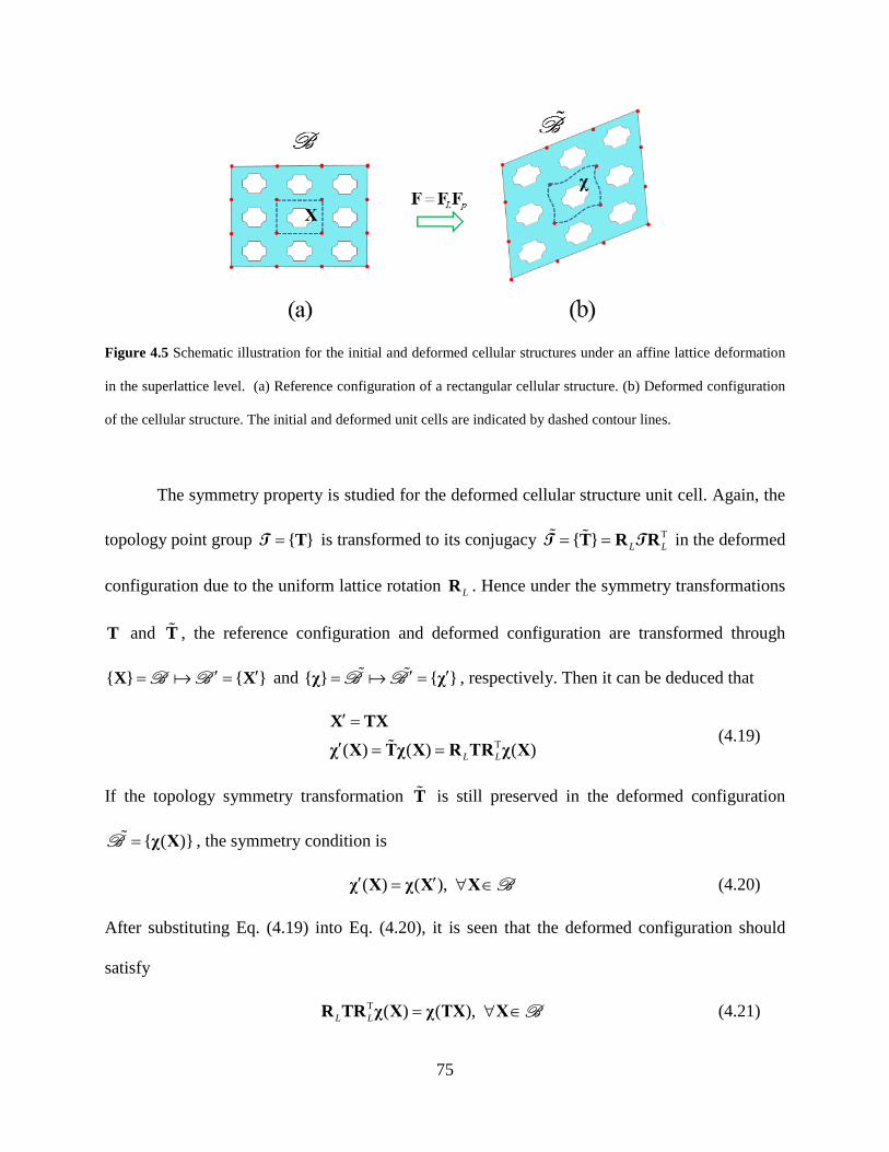
75
Figure 4.5 Schematic illustration for the initial and deformed cellular structures under an affine lattice deformation
in the superlattice level. (a) Reference configuration of a rectangular cellular structure. (b) Deformed configuration
of the cellular structure. The initial and deformed unit cells are indicated by dashed contour lines.
The symmetry property is studied for the deformed cellular structure unit cell. Again, the
topology point group { }= TT is transformed to its conjugacy T{ } L L= =T R RT T in the deformed
configuration due to the uniform lattice rotation LR . Hence under the symmetry transformations
T and T , the reference configuration and deformed configuration are transformed through
{ } { }′ ′= =X XB B and { } { }′ ′= =χ χ
B B , respectively. Then it can be deduced that
T( ) ( ) ( )L L
′ =
′ = =
X TXχ X Tχ X R TR χ X
(4.19)
If the topology symmetry transformation T is still preserved in the deformed configuration
{ ( )}= χ XB , the symmetry condition is
( ) ( ),′ ′= ∀ ∈χ X χ X X B (4.20)
After substituting Eq. (4.19) into Eq. (4.20), it is seen that the deformed configuration should
satisfy
T ( ) ( ),L L = ∀ ∈R TR χ X χ TX X B (4.21)
76
Further, taking a first order derivative to X in Eq. (4.21) and utilizing Eq. (4.17) give rise to
T T T( ) ( ) ,L L= ∀ ∈R F TX TR F X T X B (4.22)
Equation (4.22) is the fundamental equation to examine whether the deformation gradient ( )F X
preserves the topology symmetry of the cellular structure or not.
The symmetry condition of the deformation gradient ( )F X is equivalent to two separated
conditions by using the decomposition in Eq. (4.17). After substituting Eq. (4.17) into Eq. (4.22),
we obtain
T( ) ( ) ,L p L p= ∀ ∈U F TX TU F X T X B (4.23)
By substituting Eq. (4.18) into Eq. (4.23) and considering the relation ( )p L =F TX I implied by
Eq. (4.18), the symmetry of the lattice points LX requires that
TL L=U TU T (4.24)
Equation (4.24) indicates that the lattice stretch tensor LU should be form-invariant under the
symmetry operation∀ ∈T T if the lattice points are still symmetric after deformation, while the
uniform lattice rotation LR does not affect the symmetry. The formula in Eq. (4.24) was derived
by Coleman and Noll [141] in another context. Obviously, a uniform dilation deformation, i.e.
L λ=U I with λ as a stretching factor, would not affect the symmetry condition in Eq. (4.24).
The topology symmetry condition of a cellular structure is more complex than Eq. (4.24) due to
the existence of the periodic non-affine deformation pF . After eliminating LU in Eq. (4.23) by
using Eq. (4.24), the symmetry condition forces the periodic deformation field to satisfy
T( ) ( ) ,p p= ∀ ∈F TX TF X T X B (4.25)

77
Thus Eq. (4.25) indicates that the periodic deformation gradient field should be form-invariant
under the topology symmetry operation ∀ ∈T T .
Further, the symmetry preserving strain field can also be derived. Taking the Green strain
tensor field T( ) [ ( ) ( ) ] 2= −E X F X F X I [137] as an example, it satisfies
T
T T
T
( ) [ ( ) ( ) ] 2[ ( ) ( ) ] 2
( ) ,
= −
= −
= ∀ ∈
E TX F TX F TX IT F X F X I TTE X T X B
(4.26)
Figure 4.6 shows an example [127] of how symmetry breaking occurs when the strain field does
not satisfy the symmetry condition in Eq. (4.26). In this case, Eq. (4.24) is still valid while Eqs.
(4.25) and (4.26) are violated. In fact, the strain field does not preserve the 4mm topology
symmetry of the original configuration since the deformed configuration has a topology point
group of 2mm . This strain-induced symmetry breaking phenomenon has been utilized to tune
the phonon propagation behavior in the phononic crystals.
Figure 4.6 Symmetry breaking of a cellular structure induced by deformation. (a) Undeformed configuration. (b)
Deformed configuration. λ is the uniform stretch factor. The images are adapted from [127] with permission.
(a) =1λ (b) =0.8λ

78
4.4.3 Material symmetry breaking in small deformation
The material symmetry of the level 2 is studied for cellular structures. During the deformation
process ( )X χ X , the material point group field also changes as ( ) ( )X χM M , which is
usually hard to determine analytically. According to Eq. (4.4), The material symmetry of the
field ( )χM requires that
T( ) ( ) , and= ∀ ∈ ∀ ∈Gχ G χ G G χ BM M G (4.27)
where TL L= R RG G ( ≤ G T ) is the overall point group after the affine lattice deformation LF .
In small deformation cases, ( )χM could be determined since only symmetry breaking
occurs in the local configuration. The polar decomposition ( ) ( ) ( )=F X R X U X is introduced,
where ( )R X and ( )U X are the rotation and stretch tensors. For small deformation case,
symmetry breaking may occur and the material point group ( ( ))χ XM of the deformed material
is [141]
T T( ( )) : { ( ) ( ) , for and }= = ∀ ∈ ∀ ∈χ X RMR U X MU X M M X BM | M (4.28)
On the other hand, the material symmetry evolution is quite complex and almost intractable for
large deformation cases, which should be paid careful attention to.
4.5 SUMMARY
Point group symmetry is one of the most important and fundamental properties of anisotropic
materials, which is directly related to their physical properties and useful for material modeling.
79
Hence, it is quite necessary to develop a point group symmetry theory for cellular structures in
response to the second question raised in Section 1.3. However, the symmetry of cellular
structures is more complicated than single crystals due to the multilevel structural features within
a cellular structure unit cell. Specifically, the cellular structures require both topology symmetry
and material symmetry in one unit cell. To address this issue, a unified theoretical framework is
established to describe and determine the overall point group of cellular structures. Current work
reveals that the point group symmetry of cellular structures can be described by the invariant (or
form-invariant) of a material type field and a material point group field. This is significantly
different from the symmetry of single crystals, which only requires the invariant of the material
type field. The proposed theory is applied to several examples to show the symmetry
characteristics of cellular structures, especially the ones fabricated by 3D printing. In addition,
the symmetry evolution of deformed cellular structures is also investigated with an emphasis on
the deformation-induced symmetry breaking for small strain cases. The proposed theory will
provide theoretical foundation for characterizing the physical properties of cellular structures and
offer some guidance in designing tunable cellular structures by employing symmetry breaking.

80
5.0 MODELING 3D PRINTED PHOTOPOLYMERS AND CELLULAR
STRUCTURES
5.1 INTRODUCTION
The photopolymerization based technology plays a dominant role in manufacturing the 3D
printed polymeric parts with high quality. The representative techniques include SLA, PolyJet,
and multiphoton lithography, which fuse the monomers and oligomers together by using UV
light or laser layer by layer. These techniques usually produce parts with high resolution but low
distortion. However, a critical and common issue of these techniques is that the photopolymer
component exhibits strong printing direction effect [59, 60] inherited from the layer-wise
processing feature. As a result, the deformation and failure of 3D printed cellular structures will
depend on both structural orientation and printing direction. Hence, there is a strong demand to
develop advanced material models to characterize the printing direction effect and predict the
deformation and failure of 3D printed polymeric structures.
The inelastic deformation of glassy polymers usually undergoes initial yielding, strain
softening, and subsequent hardening [143, 144]. In early years, a seminal model of glassy
polymers was developed by Parks, et al. [145] to describe these features and was later on
generalized by Boyce, et al. [144] to include the effects of strain rate, pressure, and temperature.
After that, this framework was further developed by a variety of researchers. For example, a

81
notable contribution was the adoption of the eight-chain model [146, 147] to characterize the
backstress evolution, which has a simple form but good accuracy. In addition, a different 1D
rheological model was introduced by Bergström and Boyce [148], which is also quite popular
nowadays. Other development includes modifying the network model [149-151], generalizing
the rheological model [152-155], considering thermo-mechanical coupling [156-158], and
applying the models for new materials [52, 159], which can be found in these literature and the
references therein. Unfortunately, these models still suffer from some limitations when applied to
3D printed photopolymers. On the one hand, these models are usually devised for isotropic
glassy polymers, e.g. isotropic elastic tensor and von Mises stress are used, which do not
consider the material anisotropy induced by the printing direction effect. On the other hand, these
models usually adopt an associated flow rule, which leads to unphysical volume dilatation when
the material is pressure sensitive [160]. Therefore, one aim of this chapter is to develop a
transversely isotropic inelastic model for photopolymers to tackle these two critical problems,
which has improved accuracy compared with the isotropic model used for photopolymers [52].
The 3D printed photopolymers usually show orientation-dependent failure behavior, that
is, the interface between two printing layers is usually weaker than the intra-layer strength under
tensile loading. A macroscopic failure criterion is useful for engineering analysis to estimate the
material and structure failure [161]. Some representative stress-based failure criteria are, for
instance, the Tsai-Wu criterion [162] and Hashin criterion [163], which were originally
developed for fiber composites and have been widely used. However, these stress-based failure
criteria are not applicable when the material exhibits strain softening, in which case one stress
value may correspond to several strain values. In contrast, the failure criteria [164, 165]
formulated in the strain space can overcome this issue, but they are difficult to extend to

82
problems involving inelastic deformation since the strain is decomposed into elastic and inelastic
parts. Therefore, the stress-based formulation is adopted in this chapter by modifying the Tsai-
Wu criterion to handle the failure problems with strain softening. Note that a well-developed
macroscopic failure criterion is quite useful for engineering failure analysis, and indeed there is
still a lack of such model for photopolymers.
The ultimate goal of this chapter is to study the deformation and failure behavior of 3D
printed cellular structures with material anisotropy. In order to achieve this goal, a transversely
isotropic hyperelastic-viscoplastic model is established for photopolymers by considering
material anisotropy, pressure sensitivity, and rate dependence, and a failure criterion is proposed
by modifying the Tsai-Wu model. Finally, the developed material model and failure criterion are
implemented into the user subroutine (VUMAT) of the finite element software package
ABAQUS to simulate the structural response and failure of 3D printed cellular structures. The
simulation results will be compared with those obtained from experiment.
5.2 HYPERELASTIC-VISCOPLASTIC MODEL OF PHOTOPOLYMERS
5.2.1 Kinematics of finite deformation
The inelastic deformation of the glassy polymers is studied in the finite deformation scenario.
The deformation of a continuum body is illustrated in Figure 5.1. The finite strain deformation of
this deformed body is described by the deformation gradient F , which maps a material point X
of the reference configuration 30 ⊂B R to a spatial point ( )χ X in the current configuration
3⊂B R , as

83
∂=∂χFX
(5.1)
The corresponding velocity gradient, L , is given by
1−∂= = = +∂χL FF D Wχ
(5.2)
where the dot indicates the first order time derivative. In Eq. (5.2), D and W are the symmetric
part and skew part of L , respectively, which represent the stretching rate tensor and spin tensor.
For finite strain deformation incorporating plasticity, the deformation gradient is usually
decomposed into two parts [166], as
e p=F F F (5.3)
Since the choice of the relaxed configuration 3p ⊂B R is not unique, we adopt a particular
relaxed configuration so that eF is always symmetric, i.e. e e=F V , where eV is the left stretch
tensor of eF [144]. Further, the plastic deformation gradient pF can also be decomposed into
two parts, as
p p p p p= =F R U V R (5.4)
where pR is the rotation tensor, pU is the right stretch tensor, and p p p pT=V R U R is the left
stretch tensor. The decomposition in Eq. (5.4) is also illustrated in Fig. 1 by introducing an
intermediate configuration 3ps ⊂B R with plastic stretch deformation only.
The velocity gradient in Eq. (5.2) can be rewritten in the following form after the
multiplicative decomposition of the deformation gradient, as
e e p e 1−= +L L F L F (5.5)
The term pL in Eq. (5.5) is the plastic velocity gradient, which is defined as
p p p 1 p p−= = +L F F D W (5.6)

84
where pD and pW are the plastic stretching rate and plastic spin tensor, respectively. In order to
guarantee the symmetry of the elastic deformation gradient eF , the plastic spin pW in Eq. (5.6)
should satisfy the following relation [160, 167], as
p p p p 1 p 2 p p p p p p 2 p p p 2
p p p p p p
( ) [ ( ) ( )
( ) ]
I II III I I−= − − − −
+ −
W V D D V V D D VV V D D V V
(5.7)
where p , pI II , and pIII are the three invariants of pV , as
p p
p p2 p2
p p
tr
[ tr( )] 2
det
III IIII
=
= −
=
VV
V (5.8)
where tr( ) and det( ) indicate the trace and determinant of a tensor, respectively.
Figure 5.1 Multiplicative decomposition F = FeFp of the deformation gradient for a continuum body with elasto-
plastic deformation. The plastic deformation can be further decomposed into a pure stretching part and a pure
rotation part, as p p p=F R U . The symbols 0B , B , pB , and psB indicate the reference configuration, current
configuration, relaxed configuration, and plastic stretching configuration, respectively. The corresponding privileged
axes in these four configurations are denoted by 0n , n , pn , and psn , respectively.

85
The main difference between the kinematic relations of isotropic and anisotropic bodies
is that the material anisotropy, usually characterized by the material axes, should be considered
for the latter. For the 3D printed photopolymers, we assume that the material is transversely
isotropic in the reference configuration since they usually have the lamellar structure. Hence, it is
natural to take the printing direction as the material’s privileged axis, i.e. 0n in the reference
configuration 0B of Figure 5.1. The evolution of the privileged axis 0n is especially important
to the constitutive modeling in the finite deformation scenario. As shown in Figure 5.1, the effect
of the plastic stretch pU on the evolution of the privileged axis 0n is usually assumed to be
unchanged during the plastic stretch process, i.e. ps 0=n n . Therefore, the privileged axis pn in
the relaxed configuration pB is only affected by the plastic rotation pR , as
p p 0=n R n (5.9)
In addition, the rate form of Eq. (5.9) is derived as
p p 0 p p= =n R n W n
(5.10)
where p p pT=W R R is the material spin tensor. Actually, the effect of the plastic stretch pU on
the material anisotropy evolution can be incorporated into the constitutive law by adding a
vector/tensor type state variable representing the texture change [160, 168]. However, this
approach would increase the complexity of the resulting model, which is usually difficult to fit
through experiment. In practice, the assumption stated in Eq. (5.9) is more popular.
The anisotropy of the transversely isotropic materials is represented by the structural
tensor, which evolves with the deformation. In the reference configuration 0B , the structural
tensor is defined as
0 0 0= ⊗M n n (5.11)

86
Correspondingly, this structural tensor in the relaxed configuration pB is defined as
p p p= ⊗M n n (5.12)
It is easy to verify from Eq. (5.11) and Eq. (5.12) that p p 0 pT=M R M R .
5.2.2 Material model
The 3D printed photopolymers behave like many other glassy polymers, which usually undergo
elastic response, yielding, strain softening, and successive hardening due to the stretching of
polymer chains at different deformation stages. In order to capture all these behaviors, a
hyperelastic-viscoplastic polymer model is shown in Figure 5.2. The 1D rheological chain in
Figure 5.2 (a) is frequently used to model the glassy polymer response [147], which consists an
elastic spring, a hyperelastic spring, and a viscoplastic element. The hyperelastic spring is used
to model the backstress evolution due to the hardening of the glassy polymer under large
inelastic strain, as shown in Figure 5.2 (b). Finally, the equilibrium of the stress state is
formulated in the relaxed configuration pB in this work.
The linear elastic deformation eF of the polymer is modeled by the elastic spring in
Figure 5.2 (a). Notice that the elastic deformation is usually quite small. Hence, the elastic stress
eσ in the relaxed configuration pB is determined as
e e e:=σ E (5.13)

87
Figure 5.2 Schematic illustration of the hyperelastic-viscoplastic model. (a) A one-dimensional rheological model
for the transversely isotropic photopolymer. (b) A typical stress-strain curve for glassy polymers. The backstress is
modeled by a hyperelastic spring.
where e eT e( ) 2= −E F F I is the elastic Green strain tensor, e is the fourth order elastic tensor
in the relaxed configuration pB , and “:” is the double dot product of the tensors. The explicit
form of e is derived as follows. It is assumed that the plastic stretch deformation pU does not
change the elastic response of the polymer. Therefore, e can be obtained via a rotation
transformation pR to the elastic tensor in the reference configuration 0B , as
e 1 p p p ppijkl abcd ia jb kc ldJ R R R R−= (5.14)
where pp detJ = U accounts for the plastic volume change. The explicit form of in Eq. (5.14)
is expressed in the following form for transversely isotropic materials [169], as
0 0 0 002 ( ) 2( )λ µ α µ µ β⊥ ⊥= ⊗ + + ⊗ + ⊗ + − + ⊗I I M I I M M M
(5.15)

88
where λ , µ
, µ⊥ , α , and β are five independent elastic constants, ijkl ik jlδ δ= is the fourth-
order identity tensor, and 0 00( )ijkl im jmkl jm miklM M= + .
Further, a more convenient form of the stress eσ in Eq. (5.13) can be written as
e 1 e e p e e p
p
p e e p p e p
{ (tr ) 2 [( : ) (tr ) ]
2( )( ) ( : ) }
J λ µ α
µ µ β
−⊥
⊥
= + + +
+ − + +
σ E I E M E I E M
M E E M M E M
(5.16)
In addition, the Cauchy stress σ in the current configuration B can be determined from Eq.
(5.13) or Eq. (5.16) after a push-forward transformation, as
1 e e eTeJ −=σ F σ F (5.17)
where ee detJ = V is the elastic volume change. Equation (5.17) is quite useful for the
implementation of the material model in the finite element algorithms.
It is worthwhile to mention that the spatial Hencky strain e eh ln=E V and the Kirchhoff
stress eK eJ=τ σ are usually used in the literature to describe the isotropic elastic deformation of
glassy polymers [144]. However, this convention is inappropriate for anisotropic cases because
ehE and e
Kσ are not a work-conjugate pair in general [170]. Therefore, we adopt the Green strain
eE instead of ehE in this work.
The material hardening of the glassy polymer is modeled through the evolution of the
backstress bσ derived from a hyperelastic model. Note that the polymer is transversely isotropic
in the reference configuration 0B . Therefore, the strain energy function of the hyperelastic
spring has a general form of
p 0 p p p p p1 2 3 4 5( , ) ( , , , , )I I I I IΦ = ΦC M (5.18)

89
where p p2=C U is the right Cauchy-Green tensor, p ( 1, 2, ,5)iI i = are the five invariants
defined as [134]
p p1p p2 p22 1p p 23 p
p 0 p4p 0 p25
tr
[ tr( )] 2
det
:
:
II II J
II
=
= −
= =
=
=
CC
C
M CM C
(5.19)
A variety of strain energy functions have been proposed in the literature [171] for Eq.
(5.18). In this work, the following form of hyperelastic strain energy is chosen, as
2 p 2p 4
sinh( 1) ln ( 1)2 4
chch ch
ch
J n n Iβκ µµ β λβ
Φ = − + − + −
(5.20)
where κ , µ , n , and µ are four hyperelastic constants. The first term of Eq. (5.20) is the
volume dilation energy, the second term is adapted from the eight-chain model [146] for the
distortion energy, and the last term is the standard reinforcing model to characterize the
anisotropy [171, 172] induced by the printing direction effect. Moreover, the terms chλ and chβ
in Eq. (5.20) are defined as
p12 3p
1
3ch
chch
IJ
n
λ
λβ −
=
=
L
(5.21)
where ( ) coth 1ch ch chβ β β= −L is the Langevin function.
The derivation of the backstress bσ is straightforward once a proper hyperelastic strain
energy function is given. Following a procedure outlined by Ogden [172], the backstress bσ in
the relaxed configuration pB is determined as
90
b 1 p p pp 3p p p
1 3 4
p 1 p pp p 45 3
p
2 2 2
( 1) ( 1)3
chdev
ch
J II I I
nJ J IJµ βκ µ
λ
−
−
∂Φ ∂Φ ∂Φ= + + ∂ ∂ ∂
= − + + −
σ B I M
I B M
(5.22)
where p p pT=B F F is the left Cauchy-Green tensor and the subscript ‘dev’ means the deviatoric
part of a tensor. Note that Eq. (5.22) satisfies the stress-free condition when p =F I .
The experimental testing indicates that the inelastic deformation of 3D printed
photopolymers is rate-dependent, pressure sensitive, and orientation-dependent. Therefore, the
viscoplastic element is modeled to incorporate all these factors. The driving stress σ for the
viscoplastic flow is derived from the equilibrium of the 1D rheological network in Figure 5.2 (a),
as
e b= −σ σ σ (5.23)
where eσ and bσ are defined in Eq. (5.13) and Eq. (5.22), respectively. In the case that the
material is transversely isotropic and pressure sensitive, the equivalent stress is defined in a
modified Hill form by incorporating the Bauschinger effect [173-175], as
2 2 p p 2 p1 2 3 4 5tr( ) tr ( ) tr( ) tr( ) trdev dev dev deva a a a aτ = + + + +σ M σ M σ M σ σ (5.24)
where ( 1, 2, ,5)ia i = are five dimensionless yield constants and pM is the structural tensor
defined in Eq. (5.12).
5.2.3 Non-associated flow rule
A non-associated flow rule is used since glassy polymers are pressure sensitive, otherwise
unphysical plastic volume dilatation will occur [160, 176]. The flow potential is chosen as
91
p( , )g J pψ τ= + (5.25)
where g is an unknown function to be determined and p is the equivalent pressure defined as
p4 5
5
1 [ tr( ) tr ]3 devp a aa
= +M σ σ (5.26)
where the term related to 4a is introduced to account for the anisotropy of the polymer. Note that
the pressure in Eq. (5.26) is positive in tension and negative in compression.
The evolution of the plastic deformation rate is
p pγ=D N (5.27)
where pγ and N are the amplitude and direction of the viscoplastic flow, respectively. The flow
direction tensor N is obtained from the derivative of the non-associated flow potential in Eq.
(5.25), as
p p p p
1 2 32 2 p p 2
1 2 3
p4 5
5
tr( ) 0.5 ( )tr( ) tr ( ) tr( )
11 ( )3
dev dev dev dev dev dev
dev dev dev
dev
a a aa a a
g a aa p
ψ∂=∂
+ + +=
+ +
∂+ + + ∂
Nσσ M σ M M σ σ M
σ M σ M σ
M I
(5.28)
Then based on Eq. (5.27) and Eq. (5.28), the plastic volume change rate is derived as
pp p
pp
p5 p
tr
tr
3
J J
J
ga Jp
γ
γ
=
=
∂= + ∂
D
N
(5.29)
It can be seen from Eq. (5.29) that the term g p∂ ∂ introduced by the non-associated flow rule is
quite important for the plastic volumetric deformation. Otherwise, pJ is always positive (or
negative) if an associated flow rule is used ( 0g ≡ ), which results in an unreasonable plastic

92
dilatation. The significance of the non-associated flow rule has also been recognized in the
literature [160] for other pressure-sensitive materials like granular materials, rocks, foams, etc.
The explicit form of p( , )g J p should be determined by experiment, which is quite challenging.
Therefore, it is assumed that the plastic volume change rate pJ is a linear function with respect
to the equivalent pressure p . As a result, the term enclosed in the bracket of Eq. (5.29) is written
as
5p
3 g pap κ∂
+ =∂
(5.30)
where pκ is a plastic dilatancy parameter. Finally, the plastic flow direction N can also be
derived by substituting Eq. (5.30) into Eq. (5.28). In addition, the plastic volume change rate is
obtained from Eq. (5.29), as
p
pp
p
JJ p
γκ
=
(5.31)
The equivalent plastic flow rate pγ is taken as the following form:
p0
B
exp 1Gk s
τγ γϑ
∆ = − −
(5.32)
where 0γ is a pre-exponential factor, G∆ is the zero stress level activation energy, s is the
athermal shear strength, Bk is the Boltzmann constant, and ϑ is the absolute temperature. Other
types of flow equations can also be found in the literature [177, 178], which usually have
different indices. The strain softening is modelled by introducing a preferred state ss so that the
athermal threshold stress evolves in the following way, as [144]
p
s
1 ss hs
γ
= −
(5.33)

93
where h is the softening slope and the initial condition is 0s s= when p 0γ = . It should be
mentioned that an additional term was introduced in some literature [144] to take into account
the effect of pressure on the athermal shear threshold stress. Nevertheless, this correction is not
necessary any more in this work since the effect of pressure on the peak yield stresses has
already been considered in the equivalent stress τ defined in Eq. (5.24). So far, the plastic
stretching rate pD in Eq. (5.27) can be determined by using Eqs. (5.32), (5.33), and (5.28) and
the rate type constitutive model is completed.
A final remark on the constitutive model is that the energy dissipation rate pW should
always be non-negative according to the second law of thermodynamics, i.e.
p p p: 0gW pp
γ τ ∂
≡ = + ≥ ∂ σ D
(5.34)
Roughly speaking, the coefficient term g p∂ ∂ can be interpreted as the pressure-dependent
internal friction of the material. In addition, based on Eq. (5.34), the condition p 0W ≥ requires
that 0p g pτ + ∂ ∂ ≥ , which should be checked when fitting the parameters.
5.3 FAILURE CRITERION OF PHOTOPOLYMERS
The Tsai-Wu failure criterion [162] is adopted to predict the macroscopic failure of 3D printed
photopolymers. However, the original Tsai-Wu failure criterion does not apply for materials with
strain softening and hence is being modified in this work. In general, the failure criterion should
be expressed in terms of the stress eσ , structural tensor pM , accumulated plastic deformation

94
pγ , flow rate pγ , temperature ϑ , and/or other internal variables. Hence, the general failure
criterion is
e p p p( , , , , , ) 1f γ γ ϑ ≤σ M (5.35)
The Tsai-Wu failure criterion is a special case of Eq. (5.35), which is expressed in the following
form, as
2 24 6 4 6
4 6 8 72 2
1 1 1 1 1 1
1 1 1
K K K KT C T C T C T C
F K K K KS S
⊥ ⊥ ⊥ ⊥
⊥⊥
− + − + +
+ + + ≤
(5.36)
where T
, C
, and S
are the out-of-plane tension, compression, and shear strength along the
printing direction, T⊥ , C⊥ , and S⊥ are the in-plane tension, compression, and shear strength,
and F ⊥ is the coefficient of a mixture term. The stress invariants ( 1, 2, ,8)iK i = in Eq. (5.36)
are defined as
e1
2 e22 1
p e4
p e25
6 1 42
7 5 4
8 4 6 2 7
tr
[ tr( )] 2
:
:
KK KKKK K KK K KK K K K K
=
= −
=
== −
= −= − −
σσ
M σM σ (5.37)
In the special case that the material failure is dominated by tension, the failure criterion in Eq.
(5.36) could be simplified by assuming C →∞
, C⊥ →∞ , and S⊥ →∞ , as
6 744 6 2 1K KK F K K
T T S⊥⊥
+ + + ≤
(5.38)

95
Generally speaking, these failure constants should be functions of the accumulated plastic strain
pγ , flow rate pγ , temperature ϑ , etc. However, we only consider that the in-plane tensile
strength decays during the plastic deformation. Therefore, T⊥ is prescribed as
p1 0 1 2( ) exp( )T T T T T γ⊥ ⊥ ⊥ ⊥ ⊥= + − − (5.39)
where 0T⊥ is the initial tensile strength, 1 0T⊥ > is the target strength, and 2 0T⊥ > is the
decaying rate (see Figure 5.3). Indeed, other failure constants can also be expressed in similar
forms, while we assume that the other three constants do not change with the plastic deformation
due to the brittle nature of the photopolymer in the 3D printing direction. The first two terms in
Eq. (5.38) are the dominant terms which dictate the tensile failure in 3D printed photopolymers,
while the other two terms are introduced to incorporate the failure mode coupling and shear
effect.
Figure 5.3 Schematic illustration of the tensile failure occurring in the strain softening process of a material. The
tensile strength is a decaying function with respect to the plastic flow instead of a constant in the stress space.
It should be noted that the macroscopic failure criterion depends much on the knowledge
of failure modes observed in experiment and the available data tested under certain conditions. In

96
reality, the failure process includes damage accumulation and crack growth, which requires
considerable effort and detailed analysis by using damage mechanics, nonlinear fracture
mechanics, and even more advanced techniques [179-181]. This kind of failure criterion based
analysis can only provide some engineering design guidance rather than predicting the failure
process accurately.
5.4 EXPERIMENTAL TEST OF PHOTOPOLYMERS
5.4.1 Identification of parameters
All material constants are determined by conducting uniaxial tension and compression tests on
specimens printed along different orientations. As shown in Figure 5.4, all specimens are tested
along the 2x direction in the Cartesian coordinate system 1 2 3ox x x . The unit vectors of the three
coordinate axes are designated as 1e , 2e , and 3e , respectively. The printing direction
01 2cos sinθ θ= +n e e is perpendicular to the axis 3x and has an angle of θ with respect to the
axis 1x . Therefore, 0θ °= indicates the in-plane direction, while 90θ °= indicates the out-of-
plane or printing direction. Given that 0n is prescribed, the matrix form of the structural tensor in
the reference configuration can be obtained from Eq. (5.11), as
2
0 2
cos sin cos 0sin cos sin 0
0 0 0
θ θ θθ θ θ
=
M (5.40)
An overview of calibration procedure of the material constants in the model is introduced
first. For the uniaxial testing simulation, the deformation can be obtained through the time

97
integration of the constitutive law by using the backward Euler algorithm and assuming a set of
trial material constants. After that, the trial material constants are then optimized iteratively by
using the Hooke-Jeeves pattern search method [182] to minimize the fitting error. Note that this
Hooke-Jeeves method does not require any gradient information of the target function, which is
quite convenient. The initial trial values of the materials constants are estimated as follows.
Figure 5.4 Schematic illustration of the material coordinate system and printing direction. (a) The testing direction
and printing direction of the uniaxial testing specimens. The isotropic plane is indicated by the dashed elliptical
cross section. (b) Manufacturing setup for the tensile specimen. The printing direction is indicated by the arrow. The
compression testing specimens are arranged in a similar way.
The five elastic constants in Eq. (5.15) can be fitted from the linear responses of the
material. In the Voigt notation, the matrix form of the elastic tensor is
T0θ θ == Q Q (5.41)
where
98
0
2 4 2 0 0 02 0 0 0
2 0 0 00 0 0 0 00 0 0 0 00 0 0 0 0
θ
λ α β µ µ λ α λ αλ α λ µ λλ α λ λ µ
µµ
µ
⊥
⊥
⊥=
⊥
+ + + − + + + + + +
=
(5.42)
2 2
2 2
cos sin 0 0 0 sin 2sin cos 0 0 0 sin 2
0 0 1 0 0 00 0 0 cos sin 00 0 0 sin cos 0
cos sin cos sin 0 0 0 cos 2
θ θ θθ θ θ
θ θθ θ
θ θ θ θ θ
−
= −
−
Q (5.43)
Thus, once a uniaxial stress state e e2 2σ= ⊗σ e e is given, the corresponding elastic strain field
can be readily derived from Eq. (5.13), which can be used to obtain the directional elastic
moduli. Thereafter, the five elastic constants can be calculated by fitting the directional elastic
moduli from the tension and compression testing along different printing directions.
The five yield constants in Eq. (5.24) can be estimated in the following way. For a given
uniaxial yield stress state Y 2 2σ= ⊗σ e e , the equivalent stress τ in Eq. (5.24) is prescribed to be
Y 03
θτ σ +
== as a reference stress value. Thus, it is obtained that the yield stress for an arbitrary
orientation θ is
Y
2 2 2 2Y 1 2 3 4 50
36 (1 3sin ) (1 3sin ) (1 3sin ) 3a a a a a
θ
θ
σ
σ θ θ θ
±
+
=
=± + − + + − − +
(5.44)
where the superscript + (or –) sign means the tension (or compression) condition. As indicated
by Eq. (5.44), there are two yield stresses for each orientation, which correspond to the tensile
and compressive yield stresses, respectively. Hence, the five yield constants can be obtained by
fitting the yield stress data obtained from the uniaxial tension and compression tests along the

99
three directions 0 , 45θ = , and 90 . The estimation of the six viscoplastic flow constants can
follow a procedure suggested in [159]. In addition, the four hyperelastic constants should be
determined together with other constants. Finally, the optimization of trial material constants can
be conducted by minimizing the fitting error between the simulation stress-strain curves and
experimental data.
Following the procedure introduced above, the 20 material constants and 6 failure
constants for the VeroWhitePlus (VW) photopolymer is listed in Table 5.1.
5.4.2 Manufacturing of specimens
All the test specimens are fabricated from the VW photopolymer by using the Objet260 Connex
3D printer. Both of the UV lamps are used to cure the photopolymer in order to achieve the best
mechanical performance. After printing is done, the manufactured specimens are cleaned up by
using the water jet to remove the support resin. Note that the specimens are not soaked in the
NaOH solution to avoid any changes of the mechanical property.
The tension and compression specimens are manufactured along different printing
directions in the fashion shown in Figure 5.4 (b). Flat tensile specimens are manufactured with a
total length of 100 mm and a thickness of 4.1 mm. The gauge section of the tensile specimen is
25.4 mm long and 8.2 mm wide. In contrast, the compression specimens are in cylindrical shape
with a diameter of 10 mm and a height of 8 mm. Note that this aspect ratio can usually avoid the
occurrence of buckling or barrel shape during the compression testing. Finally, it is worthwhile
to mention that the surfaces of the manufactured specimens are usually rough, which are
polished by sandpaper before testing.

100
Table 5.1 Material constants of the VW photopolymer manufactured by the PolyJet process
Model components Material parameters Values
elastic
λ (MPa) 3140 µ⊥ (MPa) 724 µ
(MPa) 775
α (MPa) 173 β (MPa) -62
hyperelastic
κ (MPa) 213 µ (MPa) 7 n 1.6 µ (MPa) -2.9
yield
1a 0.5455
2a -0.0550
3a 0.1749
4a 0.0343
5a 0.0672
viscoplastic
0γ (s-1) 57.9 10× G∆ (J) 191.35 10−×
0s (MPa) 110
ss (MPa) 53
h (MPa) 340
pκ (MPa) 1000
failure
T
(MPa) 42
0T⊥ (MPa) 130
1T⊥ (MPa) 50
2T⊥ 20 F ⊥ (MPa-2) 410−− S
(MPa) 110

101
5.4.3 Uniaxial testing results
Uniaxial tension and compression tests are conducted on an MTS880 system for the VW
photopolymer specimens in order to fit the material constants of the developed model. Three
different printing orientations of the specimen are considered, i.e. 0 , 45 ,θ ° °= and 90° , where θ
is the angle between the longitudinal axis of the specimen and the printing plane. In other words,
0θ °= and 90θ °= would indicate that the mechanical loading direction is perpendicular and
parallel to the printing direction of the 3D printer, respectively. In addition, the photopolymer is
tested under three different true strain rates ( 1 10.002 s , 0.01sε − −= , and 10.02 s− ) to capture the
rate-dependent behavior of the viscoplastic response. All the testing is conducted at room
temperature 295 Kϑ = . However, it was found that the temperature of the compression
cylinders may rise when they are loaded at relatively high strain rate since the thermal condition
is not ideally isothermal. Therefore, a thermal camera (FLIR SC325) is used to monitor the
temperature change of the cylinders during the compression testing. As shown in Figure 5.5, the
temperature increment ϑ∆ could reach ~ 9 K in the case of 10.02 sε −= but does not change
much for low strain rate cases, e.g. 10.002 sε −= . In contrast, the temperature rising of the flat
tensile specimens is negligible since they usually break at a low strain level.

102
Figure 5.5 Temperature rising of the cylindrical specimens during the compression testing. The data is fitted by
polynomial functions to be used for the simulation.
The uniaxial tension and compression curves of the VW photopolymer specimens are
shown in Figure 5.6 and Figure 5.7, respectively. Besides the experimental results, the stress-
strain curves are also obtained from the proposed model for comparison. Note that the measured
temperature data in Figure 5.5 is input into Eq. (5.32) during the compression simulation to
incorporate the material softening induced by the temperature rise. Overall, the proposed model
could fit the experimental results very well for both tension and compression cases and along
different specimen printing directions. The stress-strain curves are similar to other glassy
polymers, which usually have a linear elastic region, strain softening region, and successive
hardening region as the strain increases. Some remarkable features of Figure 5.6 and Figure 5.7
are noted as follows. (i) The elastic response of the VW photopolymer is transversely isotropic.
The elastic modulus along the printing direction ( 90θ °= ) is about 10% higher than that within

103
the printing plane ( 0θ °= ). Note that this anisotropic degree is dependent on the curing state of
the photopolymers. Normally, the elastic response of fully cured photopolymers shows less
anisotropy compared to partially cured photopolymers. (ii) The tensile yield stress depends
significantly on the printing direction. However, the compression yield stress does not vary much
along different directions. This is probably due to the generation and evolution of interfacial
defects [183-185] between printing layers, e.g. cavitation, bond breakage, entanglement
decohesion, etc., to be further explored by experiment. Note that these interfacial defects play an
important role under tension rather than compression. (iii) Strong pressure-sensitivity is
observed by comparing the results in Figure 5.6 with that in Figure 5.7, which shows that the
compression yield stress is usually higher than the tensile yield stress. This Bauschinger effect is
captured well by the additional pressure-related terms in Eq. (5.24). (iv) The temperature rise at
relatively high strain rates would lead to material softening. This is evidenced by the fact that the
stress gap between different strain rate cases becomes smaller with an increase of strain (see
Figure 5.7). Actually this effect would be more significant for even higher strain rate cases. (v)
The material strength is strongly dependent on the printing direction and loading condition. The
experimental data indicate that the photopolymer does not fail under compression testing. In
contrast, the material failure is dominated by the tensile stress states, especially when the printing
direction coincides with the tensile direction. As shown in Figure 5.6 (a), the in-plane tensile
behavior is ductile with considerable plastic deformation observed. However, the photopolymer
is quite brittle along the printing direction, which breaks when the stress is only about 60-70% of
the yield stress along that direction. Therefore, we can conclude that the mechanical properties
of the VW photopolymers are related to the printing direction, especially their mechanical
strength.

104
Figure 5.6 Uniaxial tensile testing results of the VW photopolymer with comparison to experimental results. The
testing is conducted under room temperature 295 Kϑ = . (a) 0θ °= . (b) 45θ °= . (c) 90θ °= . Note that θ denotes
the printing direction.
Figure 5.7 Uniaxial compression testing results of the VW photopolymer with comparison to experimental results.
The testing is conducted under room temperature 295 Kϑ = . (a) 0θ °= . (b) 45θ °= . (c) 90θ °= .
105
5.4.4 Failure criterion calibration
The tensile failure tests are conducted on tensile specimens manufactured along nine different
printing directions ( 0 ,11.25 , 22.5 , ,90θ ° ° ° °= ) to verify and calibrate the proposed failure
criterion in Eq. (5.38). All specimens are tested under the room temperature 295 Kϑ = and a
true strain rate of 10.01sε −= . The corresponding true stress and true strain values are recorded
when the material fails, which are called failure stress and failure strain, respectively. The
experimental failure data are compared with the simulation ones in Figure 5.8. It can be observed
that the theory could roughly fit the failure envelope, although there is still some variance in the
experimental failure data. Two conclusions can be drawn from Figure 5.8 regarding the failure
behavior of 3D printed glassy photopolymers. (i) The proposed failure criterion can predict the
failure of glassy polymers with strain softening. The failure stress always increases when the
printing direction increases from 0θ °= to 40θ °= . Meanwhile, the failure strain decreases,
which indicates that there exists strain softening in the material. (ii) The tested photopolymer
shows a brittle-to-ductile transition behavior, depending on the printing direction. It is seen in
Figure 5.8 (b) that the failure strain along the printing direction is much lower than the in-plane
failure strain. In addition, the failure strain envelope is in a dumbbell shape rather than a perfect
circle in the polar plot, which is quite different from isotropic materials. Note that the failure data
could also be fit into the more generalized failure criterion in Eq. (5.36) by assuming large
strength values for the failure constants C
, C⊥ , and S⊥ . However, these three values are set as
infinity for simplicity since we have not observed any compression induced failure in the
photopolymer. In addition, the failure criteria are also dependent on the loading rate and

106
temperature, which should be considered for the failure analysis if enough experimental data are
available.
Figure 5.8 Tensile failure data obtained from the experiment and simulation for the VW photopolymer with
different print directions ( 10.01 sε −= and 295 Kϑ = ). (a) Failure stress (unit: MPa). (b) Failure strain.
5.5 SIMULATION AND EXPERIMENT FOR 3D PRINTED CELLULAR
STRUCTURES
The proposed constitutive model and failure criterion are used to analyze the structural response
of 3D printed cellular structures. In order to do so, the constitutive model and failure criterion are
implemented into ABAQUS through the user material subroutine (VUMAT), and the element
deletion technique is used to predict material failure. The cellular structures are of interest
because they are widely used to design lightweight structural components [24, 186]. Particularly,
the 3D printing technology enables the manufacturing of cellular structures with complex

107
topology and excellent mechanical properties [53-56], which are usually difficult to fabricate
using conventional methods.
Figure 5.9 3D printed cellular structures by using the VW photopolymer. (a) Square cellular structure. (b) Diamond
cellular structure. The samples are either printed along the direction x1 or x2, while the compression testing is always
along x2.
Two kinds of cellular structures, square lattice and diamond lattice, are manufactured by
the Objet260 Connex printer. These two structures are actually the same but with different
orientations. However, they are named differently here according to the convention in the
literature. Again, the VW photopolymer is used to fabricate these cellular structures. As shown
in Figure 5.9 (a) and (b), the dimension of the square cellular structures and diamond cellular
structures are 52×52×20 mm3 and 56.6×56.6×20 mm3, respectively, where their depth is 20 mm.
All the ligaments are designed to be 8 mm long and 2 mm wide. In addition, all the interior
corners are filleted with a radius of 0.5 mm to avoid any local stress concentration induced by the
sharp corners. A coordinate system is established in Figure 5.9 to indicate the printing and
testing directions, which is in accordance with the coordinate system in Figure 5.4 (a).
Correspondingly, the cellular structures are either printed along the 1x or 2x direction, while the

108
compression testing is conducted along 2x . The compression testing of the cellular structures is
conducted on an MTS880 system with a nominal strain rate of 10.01sε −= and at the room
temperature 295 Kϑ = to be consistent with the testing of the photopolymer.
The uniaxial compression testing results of the square and diamond cellular structures are
shown in Figure 5.10 and Figure 5.11, respectively. The finite element simulation is performed
in ABAQUS 6.14 with the user subroutine (VUMAT) developed for the proposed model. The 4-
node plane strain element with reduced integration (CPE4R) is chosen and the explicit dynamics
solver is used. In addition, the square and diamond cellular structures are discretized into 7,514
and 7,424 quadrilateral elements, respectively. The failure simulation is performed by using the
element deletion technique, which deletes the material points (or elements) once the failure
criterion is satisfied. Although this approach for failure analysis suffers from some shortcomings,
like violating the energy conservation after deleting the material points and incapable of
predicting the failure process accurately, it is still a useful method for engineering failure
analysis due to the simplicity and convenience. Overall, the finite element analysis (FEA) results
agree well with the simulation results, especially in the linear regions. In addition, the failure
analysis can also predict the initial failure of the structures, which is usually quite challenging to
achieve. All the printed cellular structures are relatively brittle due to the weak interfaces of the
photopolymer. Thus, the structures usually fail suddenly when the peak load is achieved, except
the example in Figure 5.11 (d) - (f), which exhibits slight progressive failure. The failure of the
ligaments is mainly induced by the crack propagation along the weak interfaces, evidenced by
the simulation and experimental results. However, the overall structural responses are still quite
different between the square cellular structures (Figure 5.10) and the diamond cellular structures
(Figure 5.11). Note that the deformation is compression dominant in the former but bending

109
dominant in the latter. The load-bearing ability of the square cellular structures is still
remarkable. As shown in Figure 5.10, the vertical ligaments of the square cellular structures can
still sustain huge compression loading until the occurrence of buckling and fracture. Note that
the 3D printed photopolymer is extremely ductile under compression, although its printing
direction is brittle in tension. In contrast, the structural failure mechanism is quite different in the
diamond cellular structures, in which the external loading is sustained by the bending of
ligaments. As shown in Figure 5.11, large tensile strain is found near the joints of the diamond
cellular structures due to bending deformation, which finally leads to the failure of the joints and
immediate failure of the whole structure. By comparing Figure 5.10 and Figure 5.11, the
maximum load of the diamond cellular structures is only about 10% that of the square cellular
structures even though their overall size and relative density are very similar. This result
indicates that the overall mechanical response and failure behavior of 3D printed cellular
structures is determined by both the lattice orientation of the structure and the orientation of the
constituent material, as pointed out by Zhang and To [61] in a recent work.
This strong tension-compression asymmetry of 3D printed photopolymers also suggests
some design guidelines for 3D printed cellular structures. It is recommended to design
compression dominant structures instead of bending dominant structures to achieve the best
overall load-bearing ability, mechanical strength, and/or energy absorption behavior. Besides the
2D cellular structures shown in Figure 5.9, typical examples of the compression-dominant and
bending-dominant cellular structures are the Octet-truss structure and tetrakaidecahedron
structure, respectively [55]. Alternatively, designers can also optimize the cellular structure unit
cell by using topology optimization technique for the desired mechanical performance and
constraints [187].

110
Figure 5.10 Uniaxial compression responses of square cellular structures. Maximum principle strain (absolute
value) profiles are shown in (a) - (b) for structures printed along x1 and (d) - (e) for structures printed along x2 . The
printing direction is indicated by an arrow in the graphs. The failed elements have already been deleted to show the
cracks. (c) and (f) show the comparison of the load-displacement curves for the structures printed along x1 and x2,
respectively. The data points corresponding to the snapshots in (a), (b), (d), and (e) are indicated in (c) and (f).

111
Figure 5.11 Uniaxial compression responses of diamond cellular structures. Maximum principle strain (absolute
value) profiles are shown in (a) - (b) for structures printed along x1 and (d) - (e) for structures printed along x2. The
printing direction is indicated by an arrow in the graphs. The failed elements have already been deleted to show the
cracks. (c) and (f) show the comparison of the load-displacement curves for the structures printed along x1 and x2,
respectively. The data points corresponding to the snapshots in (a), (b), (d), and (e) are indicated in (c) and (f).

112
5.6 SUMMARY
The mechanical behavior of 3D printed cellular structures depends on the printing direction due
to the lamellar structure of the photopolymer. Thus, this chapter aims at addressing the second
question in Section 1.3 from the perspective of large inelastic deformation and failure of cellular
structures. In order to achieve this goal, a hyperelastic-viscoplastic constitutive model is
developed first for photopolymers below the glass transition temperature. The model is assumed
to be transversely isotropic in order to capture the printing direction effect, while a non-
associated flow rule is adopted since the polymer is pressure-sensitive. Along with the
constitutive model, a failure criterion is also proposed by modifying the Tsai-Wu criterion.
Specifically, the Tsai-Wu criterion is adapted to the strain softening cases by introducing a
decaying material strength in the stress space. The model is finally integrated with ABAQUS to
simulate the structural response and failure of 3D printed cellular structures. The comparison
between experiment and simulation results has been found to be very good, which suggests that
the model is able to predict the deformation of the cellular structures quite well. In addition, the
failure initiation in the cellular structures can also be predicted albeit less accurately than the
behavior before failure. The proposed model and failure criterion have promising application in
analyzing the mechanical performance of 3D printed photopolymer structures as well as other
transversely isotropic polymeric composites.

113
6.0 CONCLUSIONS
6.1 MAIN CONTRIBUTIONS
The research works presented in Chapters 2 to 5 are mainly on designing and modeling of
hierarchical materials and cellular structures inspired from biological materials. The goals are to
uncover the energy dissipation mechanisms in hierarchical materials and to model cellular
structures with material anisotropy. The key scientific contributions are as follows.
(1) Discovered the multilevel Bragg scattering mechanism in hierarchical phononic
crystals. It has long been known that the wave scattering in phononic crystals obeys the Bragg
law [71], which implies that the bandgap frequency depends on the periodicity of the structure.
Conventional phononic crystals only have a single periodicity, which results in bandgaps in a
limited range of frequencies. In contrast, the bioinspired hierarchical phononic crystals designed
in Chapter 2 have highly enhanced wave scattering behavior. It was demonstrated by the
theoretical and numerical study that the hierarchical phononic crystals can generate bandgaps in
a wide range of frequencies due to their intrinsic multilevel periodicities. Indeed, the phononic
bandgaps of the hierarchical phononic crystal are superimposed of the bandgaps generated by
each level of periodicity, which is called the multilevel Bragg scattering mechanism. This
mechanism can be employed to design phononic crystals and devices with highly enhanced wave
filtering behavior [86].

114
(2) Discovered the damping enhancement mechanism in hierarchical staggered
composites. The research on the damping behavior of staggered composites was motivated by
the relatively high damping of human cortical bone [15, 17]. The theoretical study shows that the
staggered composites could be optimized to achieve highly enhanced loss modulus, which is
proportional to the overall energy dissipation. Detailed analysis reveals that the enhanced
damping is attributed to the large shear deformation of the soft viscous matrix as a result of the
unique loading transfer characteristics of staggered composites [111]. This damping
enhancement mechanism is verified by performing experiments on three kinds of staggered
composites manufactured by 3D printing [5]. In addition, the effects of structural hierarchy and
hard phase arrangement on the damping enhancement are also discussed. The discovered
mechanism in Chapter 3 can be used to design high-performance damping composites for
engineering usage.
(3) Established a theoretical framework for the point group symmetry and
symmetry breaking of cellular structures. The point group symmetry plays an essential role in
determining the anisotropic properties of materials. However, the point group symmetry of
cellular structures was an unexplored area, although the symmetry theories of single crystals
have been well established [122, 124]. The research in Chapter 4 has established a theory to
describe and determine the point group symmetry of cellular structures with multilevel
anisotropy [61]. Specifically, the symmetry is classified into two categories, topology symmetry
and material symmetry. The overall symmetry is achieved only when both types of symmetry are
guaranteed. The symmetry breaking theory is also established to track the symmetry evolution
once the cellular structures deform. The proposed theory on point group symmetry and symmetry
breaking of cellular structures can be applied to characterize their anisotropic physical properties,

115
facilitate constitutive modeling, and guide the design and modeling of tunable materials and
structures.
(4) Developed a transversely isotropic hyperelastic-viscoplastic constitutive model
for photopolymers and applied for cellular structure analysis. The 3D printed
photopolymers exhibit a strong printing direction effect due to the layer-wise processing feature.
A hyperelastic-viscoplastic constitutive model is developed in Chapter 5 to predict the
deformation and failure of these photopolymers. The model considers pressure-sensitivity, rate-
dependence, and printing direction effect of the glassy photopolymers. In addition, a modified
Tsai-Wu type failure criterion is proposed to predict the failure of photopolymer structures.
Particularly, the modified failure criterion is applicable for materials with strain softening, which
is distinct from the original Tsai-Wu model. The constitutive model and failure criterion are used
to simulate the structural response and failure of 3D printed cellular structures. The experimental
and simulation results indicate that the mechanical behavior of 3D printed cellular structures
depend on both structural orientation and printing direction. The proposed model can be used for
3D printed photopolymers and other transversely isotropic polymers and composites.
6.2 FUTURE WORKS
Advanced composite and structure design is a fruitful and exciting area to explore, especially
when it is combined with the modern manufacturing technologies like 3D printing. Some future
works can be toward, but are not limited to, the following directions.
(1) Hierarchical acoustic materials with local resonance effect. There are mainly two
dominating mechanisms to generate bandgaps in acoustic materials, i.e. Bragg scattering and

116
local resonance [67, 188]. The multilevel Bragg scattering mechanism has been discovered in
Chapter 2 for the hierarchical phononic crystals. Thus the question is: Can hierarchical phononic
crystals be designed to exhibit multilevel local resonance ? If this is realized, one will be able to
design phononic crystals with multiple bandgaps at low frequency range, which is challenging
but highly desired in acoustic engineering.
(2) Damping composite design and fabrication. Chapter 2 has presented a way to
design composites with highly enhanced damping behavior by adopting the staggered structural
design. However, this staggered composite is highly anisotropic, which has totally different
damping behaviors along different directions. Hence, future effort can be devoted to design
isotropic composites with enhanced damping behavior, which is more robust and useful for
engineering application purpose. In addition, the manufacturing of the staggered composites is
still hindered by the current technology. For example, it is still hard to manufacture high
resolution composites with structural features in microscale. In addition, it is also difficult to
manufacture metal/ceramic with polymer together in a designed pattern, which limits the
fabrication of advanced composites with high performance.
(3) Symmetry evolution and control in tunable materials and structures. A typical
type of tunable materials [56, 127, 189] are soft cellular structures with configuration evolution
under external stimulus, e.g. loading, electric field, etc. One essential mechanism underlying
these tunable materials is the symmetry breaking, which dictates the change of physical
properties. However, the symmetry evolution after deformation is quite hard to track, although
some study in Chapter 4 has established the basic rules. Thus, it will be quite meaningful to do
more research on the symmetry evolution of deformed cellular structures, and correlate the

117
physical property change with the point group. Both theoretical and applied research can be
conducted on the tunable material design and analysis in the future.
(4) Advanced constitutive modeling for photopolymers. An advanced constitutive
model has been developed in Chapter 5 for photopolymers. The model can actually be further
extended to high strain rate and high temperature cases by incorporating thermo-mechanical
coupling and/or phase transition from glassy state to rubbery state. In addition, damage initiation
and evolution can also be integrated into the constitutive law to predict the failure process in a
more accurate way. Another meaningful research direction is to study the effect of processing
parameters on the mechanical behavior of these 3D printed photopolymers. For example, the
exposure time and intensity of the UV light will significantly affect the microstructure of the
photopolymers and hence their moduli, yield strength, and finite strain responses. These analyses
will undoubtedly assist the design of 3D printed structures for engineering usage.

118
BIBLIOGRAPHY
[1] P.-Y. Chen, J. McKittrick, and M. A. Meyers, "Biological materials: Functional adaptations and bioinspired designs," Progress in Materials Science, vol. 57, pp. 1492-1704, 2012.
[2] J. McKittrick, P.-Y. Chen, L. Tombolato, E. Novitskaya, M. Trim, G. Hirata, et al., "Energy absorbent natural materials and bioinspired design strategies: A review," Materials Science and Engineering: C, vol. 30, pp. 331-342, 2010.
[3] M. Meyers and P. Chen, Biological Materials Science: Biological Materials, Bioinspired Materials, and Biomaterials. Cambridge, UK: Cambridge University Press, 2014.
[4] P. Fratzl, "Bone fracture: When the cracks begin to show," Nature Materials, vol. 7, pp. 610-612, 2008.
[5] P. Zhang, M. A. Heyne, and A. C. To, "Biomimetic staggered composites with highly enhanced energy dissipation: Modeling, 3D printing, and testing," Journal of the Mechanics and Physics of Solids, vol. 83, pp. 285-300, 2015.
[6] J. W. Dunlop and P. Fratzl, "Biological composites," Annual Review of Materials Research, vol. 40, pp. 1-24, 2010.
[7] P.-Y. Chen, D. Toroian, P. A. Price, and J. McKittrick, "Minerals form a continuum phase in mature cancellous bone," Calcified Tissue International, vol. 88, pp. 351-361, 2011.
[8] J. Y. Rho, R. B. Ashman, and C. H. Turner, "Young's modulus of trabecular and cortical bone material: ultrasonic and microtensile measurements," Journal of Biomechanics, vol. 26, pp. 111-119, 1993.
[9] J.-Y. Rho, T. Y. Tsui, and G. M. Pharr, "Elastic properties of human cortical and trabecular lamellar bone measured by nanoindentation," Biomaterials, vol. 18, pp. 1325-1330, 1997.
[10] Z. Zhang, Y.-W. Zhang, and H. Gao, "On optimal hierarchy of load-bearing biological materials," Proceedings of the Royal Society B, vol. 278, pp. 519-525, 2011.

119
[11] K. J. Koester, J. Ager, and R. Ritchie, "The true toughness of human cortical bone measured with realistically short cracks," Nature Materials, vol. 7, pp. 672-677, 2008.
[12] E. S. Ahn, N. J. Gleason, A. Nakahira, and J. Y. Ying, "Nanostructure processing of hydroxyapatite-based bioceramics," Nano Letters, vol. 1, pp. 149-153, 2001.
[13] J. Eniwumide, R. Joseph, and K. Tanner, "Effect of particle morphology and polyethylene molecular weight on the fracture toughness of hydroxyapatite reinforced polyethylene composite," Journal of Materials Science: Materials in Medicine, vol. 15, pp. 1147-1152, 2004.
[14] S. Kobayashi, W. Kawai, and S. Wakayama, "The effect of pressure during sintering on the strength and the fracture toughness of hydroxyapatite ceramics," Journal of Materials Science: Materials in Medicine, vol. 17, pp. 1089-1093, 2006.
[15] R. Lakes, "High damping composite materials: effect of structural hierarchy," Journal of Composite Materials, vol. 36, pp. 287-297, 2002.
[16] J. F. Mano, "Viscoelastic properties of bone: Mechanical spectroscopy studies on a chicken model," Materials Science and Engineering: C, vol. 25, pp. 145-152, 2005.
[17] R. Lakes, "Viscoelastic properties of cortical bone," in Bone Mechanics Handbook, S. Cowin, Ed., 2nd ed New York: CRC Press, 2001, pp. 11.1-11.15.
[18] A. A. Abdel-Wahab, K. Alam, and V. V. Silberschmidt, "Analysis of anisotropic viscoelastoplastic properties of cortical bone tissues," Journal of the Mechanical Behavior of Biomedical Materials, vol. 4, pp. 807-820, 2011.
[19] J. Yamashita, B. R. Furman, H. R. Rawls, X. Wang, and C. Agrawal, "The use of dynamic mechanical analysis to assess the viscoelastic properties of human cortical bone," Journal of Biomedical Materials Research, vol. 58, pp. 47-53, 2001.
[20] M. E. Launey, M. J. Buehler, and R. O. Ritchie, "On the mechanistic origins of toughness in bone," Annual Review of Materials Research, vol. 40, pp. 25-53, 2010.
[21] H. Gao, "Application of fracture mechanics concepts to hierarchical biomechanics of bone and bone-like materials," International Journal of Fracture, vol. 138, pp. 101-137, 2006.
[22] H. Gao, B. Ji, I. L. Jäger, E. Arzt, and P. Fratzl, "Materials become insensitive to flaws at nanoscale: lessons from nature," Proceedings of the National Academy of Sciences, vol. 100, p. 5597, 2003.
[23] B. Ji and H. Gao, "Mechanical properties of nanostructure of biological materials," Journal of the Mechanics and Physics of Solids, vol. 52, pp. 1963-1990, 2004.
[24] L. Gibson and M. Ashby, Cellular Solids: Structure and Properties. Cambridge, UK: Cambridge University Press, 1999.

120
[25] I. Jäger and P. Fratzl, "Mineralized collagen fibrils: a mechanical model with a staggered arrangement of mineral particles," Biophysical Journal, vol. 79, pp. 1737-1746, 2000.
[26] S. Kotha, S. Kotha, and N. Guzelsu, "A shear-lag model to account for interaction effects between inclusions in composites reinforced with rectangular platelets," Composites Science and Technology, vol. 60, pp. 2147-2158, 2000.
[27] F. Bouville, E. Maire, S. Meille, B. Van de Moortèle, A. J. Stevenson, and S. Deville, "Strong, tough and stiff bioinspired ceramics from brittle constituents," Nature Materials, vol. 13, pp. 508-514, 2014.
[28] W. X. He, A. K. Rajasekharan, A. R. Tehrani‐Bagha, and M. Andersson, "Mesoscopically Ordered Bone‐Mimetic Nanocomposites," Advanced Materials, vol. 27, pp. 2260-2264, 2015.
[29] I. Corni, T. Harvey, J. Wharton, K. Stokes, F. Walsh, and R. Wood, "A review of experimental techniques to produce a nacre-like structure," Bioinspiration & Biomimetics, vol. 7, p. 031001, 2012.
[30] U. G. Wegst, H. Bai, E. Saiz, A. P. Tomsia, and R. O. Ritchie, "Bioinspired structural materials," Nature Materials, vol. 14, pp. 23-36, 2014.
[31] H.-B. Yao, H.-Y. Fang, X.-H. Wang, and S.-H. Yu, "Hierarchical assembly of micro-/nano-building blocks: bio-inspired rigid structural functional materials," Chemical Society Reviews, vol. 40, pp. 3764-3785, 2011.
[32] F. Barthelat, "Designing nacre-like materials for simultaneous stiffness, strength and toughness: Optimum materials, composition, microstructure and size," Journal of the Mechanics and Physics of Solids, vol. 73, pp. 22-37, 2014.
[33] Y. Ni, Z. Song, H. Jiang, S.-H. Yu, and L. He, "Optimization design of strong and tough nacreous nanocomposites through tuning characteristic lengths," Journal of the Mechanics and Physics of Solids, vol. 81, pp. 41-57, 2015.
[34] N. Sakhavand and R. Shahsavari, "Universal composition–structure–property maps for natural and biomimetic platelet–matrix composites and stacked heterostructures," Nature Communications, vol. 6, p. 6523, 2015.
[35] L. J. Gibson, M. F. Ashby, and B. A. Harley, Cellular Materials in Nature and Medicine. Cambridge, UK: Cambridge University Press, 2010.
[36] J. Banhart, "Manufacture, characterisation and application of cellular metals and metal foams," Progress in Materials Science, vol. 46, pp. 559-632, 2001.
[37] T. J. Lu, A. Hess, and M. Ashby, "Sound absorption in metallic foams," Journal of Applied Physics, vol. 85, pp. 7528-7539, 1999.

121
[38] A.-M. Harte, N. A. Fleck, and M. F. Ashby, "Sandwich panel design using aluminum alloy foam," Advanced Engineering Materials, vol. 2, pp. 219-222, 2000.
[39] T. Pritz, "Dynamic Young's modulus and loss factor of plastic foams for impact sound isolation," Journal of Sound and Vibration, vol. 178, pp. 315-322, 1994.
[40] S. L. Lopatnikov, B. A. Gama, M. Jahirul Haque, C. Krauthauser, J. W. Gillespie Jr, M. Guden, et al., "Dynamics of metal foam deformation during Taylor cylinder–Hopkinson bar impact experiment," Composite Structures, vol. 61, pp. 61-71, 2003.
[41] I. Elnasri, S. Pattofatto, H. Zhao, H. Tsitsiris, F. Hild, and Y. Girard, "Shock enhancement of cellular structures under impact loading: Part I Experiments," Journal of the Mechanics and Physics of Solids, vol. 55, pp. 2652-2671, 2007.
[42] I. Golovin and H.-R. Sinning, "Damping in some cellular metallic materials," Journal of Alloys and Compounds, vol. 355, pp. 2-9, 2003.
[43] J. Banhart, J. Baumeister, and M. Weber, "Damping properties of aluminium foams," Materials Science and Engineering: A, vol. 205, pp. 221-228, 1996.
[44] E. Andrews and L. Gibson, "The influence of cracks, notches and holes on the tensile strength of cellular solids," Acta Materialia, vol. 49, pp. 2975-2979, 2001.
[45] M. F. Ashby and R. M. Medalist, "The mechanical properties of cellular solids," Metallurgical Transactions A, vol. 14, pp. 1755-1769, 1983.
[46] I. Gibson, D. W. Rosen, and B. Stucker, Additive Manufacturing Technologies. New York: Springer, 2010.
[47] D. Gu, W. Meiners, K. Wissenbach, and R. Poprawe, "Laser additive manufacturing of metallic components: materials, processes and mechanisms," International Materials Reviews, vol. 57, pp. 133-164, 2012.
[48] L. E. Murr, S. M. Gaytan, D. A. Ramirez, E. Martinez, J. Hernandez, K. N. Amato, et al., "Metal fabrication by additive manufacturing using laser and electron beam melting technologies," Journal of Materials Science & Technology, vol. 28, pp. 1-14, 2012.
[49] P. J. Bártolo, Stereolithography: Materials, Processes and Applications. New York: Springer, 2011.
[50] L. S. Dimas, G. H. Bratzel, I. Eylon, and M. J. Buehler, "Tough composites inspired by mineralized natural materials: computation, 3D printing, and testing," Advanced Functional Materials, vol. 23, pp. 4629-4638, 2013.
[51] L. Murr, S. Gaytan, F. Medina, H. Lopez, E. Martinez, B. Machado, et al., "Next-generation biomedical implants using additive manufacturing of complex, cellular and functional mesh arrays," Philosophical Transactions of the Royal Society A, vol. 368, pp. 1999-2032, 2010.
122
[52] L. Wang, J. Lau, E. L. Thomas, and M. C. Boyce, "Co-continuous composite materials for stiffness, strength, and energy dissipation," Advanced Materials, vol. 23, pp. 1524-1529, 2011.
[53] B. G. Compton and J. A. Lewis, "3D‐printing of lightweight cellular composites," Advanced Materials, vol. 26, pp. 5930-5935, 2014.
[54] P. Zhang, J. Toman, Y. Yu, E. Biyikli, M. Kirca, M. Chmielus, et al., "Efficient design-optimization of variable-density hexagonal cellular structure by additive manufacturing: Theory and validation," Journal of Manufacturing Science and Engineering, vol. 137, p. 021004, 2015.
[55] X. Zheng, H. Lee, T. H. Weisgraber, M. Shusteff, J. DeOtte, E. B. Duoss, et al., "Ultralight, ultrastiff mechanical metamaterials," Science, vol. 344, pp. 1373-1377, 2014.
[56] S. H. Kang, S. Shan, A. Košmrlj, W. L. Noorduin, S. Shian, J. C. Weaver, et al., "Complex ordered patterns in mechanical instability induced geometrically frustrated triangular cellular structures," Physical Review Letters, vol. 112, p. 098701, 2014.
[57] S. Babaee, J. Shim, J. C. Weaver, E. R. Chen, N. Patel, and K. Bertoldi, "3D soft metamaterials with negative Poisson's ratio," Advanced Materials, vol. 25, pp. 5044-5049, 2013.
[58] Q. Ge, H. J. Qi, and M. L. Dunn, "Active materials by four-dimension printing," Applied Physics Letters, vol. 103, p. 131901, 2013.
[59] A. Cazón, P. Morer, and L. Matey, "PolyJet technology for product prototyping: Tensile strength and surface roughness properties," Proceedings of the Institution of Mechanical Engineers, Part B: Journal of Engineering Manufacture, vol. 228, pp. 1664-1675, 2014.
[60] D. Blanco, P. Fernandez, and A. Noriega, "Nonisotropic experimental characterization of the relaxation modulus for PolyJet manufactured parts," Journal of Materials Research, vol. 29, pp. 1876-1882, 2014.
[61] P. Zhang and A. C. To, "Point group symmetry and deformation-induced symmetry breaking of superlattice materials," Proceedings of the Royal Society A, vol. 471, p. 20150125, 2015.
[62] V. Narayanamurti, H. Störmer, M. Chin, A. Gossard, and W. Wiegmann, "Selective transmission of high-frequency phonons by a superlattice: The "dielectric" phonon filter," Physical Review Letters, vol. 43, pp. 2012-2016, 1979.
[63] M. S. Kushwaha, P. Halevi, L. Dobrzynski, and B. Djafari-Rouhani, "Acoustic band structure of periodic elastic composites," Physical Review Letters, vol. 71, pp. 2022-2025, 1993.

123
[64] T. Still, G. Gantzounis, D. Kiefer, G. Hellmann, R. Sainidou, G. Fytas, et al., "Collective hypersonic excitations in strongly multiple scattering colloids," Physical Review Letters, vol. 106, p. 175505, 2011.
[65] A. Huynh, N. Lanzillotti-Kimura, B. Jusserand, B. Perrin, A. Fainstein, M. Pascual-Winter, et al., "Subterahertz phonon dynamics in acoustic nanocavities," Physical Review Letters, vol. 97, p. 115502, 2006.
[66] M. H. Lu, L. Feng, and Y. F. Chen, "Phononic crystals and acoustic metamaterials," Materials Today, vol. 12, pp. 34-42, 2009.
[67] C. Goffaux, J. Sánchez-Dehesa, and P. Lambin, "Comparison of the sound attenuation efficiency of locally resonant materials and elastic band-gap structures," Physical Review B, vol. 70, p. 184302, 2004.
[68] S. Yang, J. Page, Z. Liu, M. Cowan, C. Chan, and P. Sheng, "Focusing of sound in a 3D phononic crystal," Physical Review Letters, vol. 93, p. 24301, 2004.
[69] B. Lee and A. To, "Enhanced absorption in one-dimensional phononic crystals with interfacial acoustic waves," Applied Physics Letters, vol. 95, p. 031911, 2009.
[70] W. Steurer and D. Sutter-Widmer, "Photonic and phononic quasicrystals," Journal of Physics D: Applied Physics, vol. 40, p. R229, 2007.
[71] R. Ramprasad and N. Shi, "Scalability of phononic crystal heterostructures," Applied Physics Letters, vol. 87, p. 111101, 2005.
[72] M. Baldassarri, H. Margolis, and E. Beniash, "Compositional determinants of mechanical properties of enamel," Journal of dental research, vol. 87, pp. 645-649, 2008.
[73] S. Bechtle, S. Habelitz, A. Klocke, T. Fett, and G. A. Schneider, "The fracture behaviour of dental enamel," Biomaterials, vol. 31, pp. 375-384, 2010.
[74] V. Imbeni, J. Kruzic, G. Marshall, S. Marshall, and R. Ritchie, "The dentin-enamel junction and the fracture of human teeth," Nature Materials, vol. 4, pp. 229-232, 2005.
[75] J. C. Weaver, G. W. Milliron, A. Miserez, K. Evans-Lutterodt, S. Herrera, I. Gallana, et al., "The stomatopod dactyl club: A formidable damage-tolerant biological hammer," Science, vol. 336, pp. 1275-1280, 2012.
[76] P. Y. Chen, A. Y. M. Lin, J. McKittrick, and M. A. Meyers, "Structure and mechanical properties of crab exoskeletons," Acta Biomaterialia, vol. 4, pp. 587-596, 2008.
[77] M. A. Meyers, P. Y. Chen, A. Y. M. Lin, and Y. Seki, "Biological materials: structure and mechanical properties," Progress in Materials Science, vol. 53, pp. 1-206, 2008.

124
[78] S. Bechtle, S. F. Ang, and G. A. Schneider, "On the mechanical properties of hierarchically structured biological materials," Biomaterials, vol. 31, pp. 6378-6385, 2010.
[79] P. Fratzl and R. Weinkamer, "Nature's hierarchical materials," Progress in Materials Science, vol. 52, pp. 1263-1334, 2007.
[80] D. Raabe, P. Romano, C. Sachs, H. Fabritius, A. Al-Sawalmih, S. B. Yi, et al., "Microstructure and crystallographic texture of the chitin–protein network in the biological composite material of the exoskeleton of the lobster 'Homarus americanus'," Materials Science and Engineering: A, vol. 421, pp. 143-153, 2006.
[81] H. O. Fabritius, C. Sachs, P. R. Triguero, and D. Raabe, "Influence of Structural Principles on the Mechanics of a Biological Fiber‐Based Composite Material with Hierarchical Organization: The Exoskeleton of the Lobster Homarus americanus," Advanced Materials, vol. 21, pp. 391-400, 2009.
[82] F. Z. Cui and J. Ge, "New observations of the hierarchical structure of human enamel, from nanoscale to microscale," Journal of Tissue Engineering and Regenerative Medicine, vol. 1, pp. 185-191, 2007.
[83] O. R. Bilal and M. I. Hussein, "Ultrawide phononic band gap for combined in-plane and out-of-plane waves," Physical Review E, vol. 84, p. 065701, 2011.
[84] K. Bertoldi and M. Boyce, "Mechanically triggered transformations of phononic band gaps in periodic elastomeric structures," Physical Review B, vol. 77, p. 052105, 2008.
[85] M. Badreddine Assouar and M. Oudich, "Dispersion curves of surface acoustic waves in a two-dimensional phononic crystal," Applied Physics Letters, vol. 99, p. 123505, 2011.
[86] P. Zhang and A. C. To, "Broadband wave filtering in bioinspired hierarchical phononic crystal," Applied Physics Letters, vol. 102, p. 121910, 2013.
[87] C. Robinson, S. Connell, J. Kirkham, R. Shore, and A. Smith, "Dental enamel - a biological ceramic: regular substructures in enamel hydroxyapatite crystals revealed by atomic force microscopy," Journal of Materials Chemistry, vol. 14, pp. 2242-2248, 2004.
[88] B. Kennett and N. Kerry, "Seismic waves in a stratified half space," Geophysical Journal of the Royal Astronomical Society, vol. 57, pp. 557-583, 1979.
[89] B. A. Auld, Acoustic Fields and Waves in Solids, 2nd ed. vol. 2. Malabar, Florida: Krieger Pub Co, 1990.
[90] S. Bechtle, H. Özcoban, E. T. Lilleodden, N. Huber, A. Schreyer, M. V. Swain, et al., "Hierarchical flexural strength of enamel: transition from brittle to damage-tolerant behaviour," Journal of The Royal Society Interface, vol. 9, pp. 1265-1274, 2012.
125
[91] P. R. Shewry, A. S. Tatham, and A. J. Bailey, Elastomeric Proteins: Structures, Biomechanical Properties, and Biological Roles. Cambridge, UK: Cambridge University Press, 2003.
[92] P. A. Deymier, Acoustic Metamaterials and Phononic Crystals. New York: Springer, 2013.
[93] R. S. Lakes, Viscoelastic Materials. Cambridge, UK: Cambridge University Press, 2009.
[94] J. Meaud, T. Sain, B. Yeom, S. J. Park, A. B. Shoultz, G. Hulbert, et al., "Simultaneously high stiffness and damping in nanoengineered microtruss composites," ACS Nano, vol. 8, pp. 3468-3475, 2014.
[95] H. Law, P. Rossiter, L. Koss, and G. Simon, "Mechanisms in damping of mechanical vibration by piezoelectric ceramic-polymer composite materials," Journal of Materials Science, vol. 30, pp. 2648-2655, 1995.
[96] G. McKnight and G. Carman, "Energy absorption and damping in magnetostrictive composites," MRS Proceedings vol. 604, pp. 267-272, 1999.
[97] M. Piedboeuf, R. Gauvin, and M. Thomas, "Damping behaviour of shape memory alloys: strain amplitude, frequency and temperature effects," Journal of Sound and Vibration, vol. 214, pp. 885-901, 1998.
[98] J. San Juan, M. L. Nó, and C. A. Schuh, "Nanoscale shape-memory alloys for ultrahigh mechanical damping," Nature Nanotechnology, vol. 4, pp. 415-419, 2009.
[99] J. Suhr, N. Koratkar, P. Keblinski, and P. Ajayan, "Viscoelasticity in carbon nanotube composites," Nature Materials, vol. 4, pp. 134-137, 2005.
[100] L. Sun, R. F. Gibson, F. Gordaninejad, and J. Suhr, "Energy absorption capability of nanocomposites: a review," Composites Science and Technology, vol. 69, pp. 2392-2409, 2009.
[101] R. Lakes, T. Lee, A. Bersie, and Y. Wang, "Extreme damping in composite materials with negative-stiffness inclusions," Nature, vol. 410, pp. 565-567, 2001.
[102] T. Jaglinski, D. Kochmann, D. Stone, and R. Lakes, "Composite materials with viscoelastic stiffness greater than diamond," Science, vol. 315, pp. 620-622, 2007.
[103] M. M. Porter, R. Imperio, M. Wen, M. A. Meyers, and J. McKittrick, "Bioinspired scaffolds with varying pore architectures and mechanical properties," Advanced Functional Materials, vol. 24, pp. 1978-1987, 2014.
[104] Y. Chen and L. Wang, "Tunable band gaps in bio-inspired periodic composites with nacre-like microstructure," Journal of Applied Physics, vol. 116, p. 063506, 2014.

126
[105] J. Yin, J. Huang, S. Zhang, H. Zhang, and B. Chen, "Ultrawide low frequency band gap of phononic crystal in nacreous composite material," Physics Letters A, vol. 378, pp. 2436-2442, 2014.
[106] M. Qwamizadeh, Z. Zhang, K. Zhou, and Y. W. Zhang, "On the relationship between the dynamic behavior and nanoscale staggered structure of the bone," Journal of the Mechanics and Physics of Solids, vol. 78, pp. 17-31, 2015.
[107] S. Kotha, Y. Li, and N. Guzelsu, "Micromechanical model of nacre tested in tension," Journal of Materials Science, vol. 36, pp. 2001-2007, 2001.
[108] F. Barthelat and R. Rabiei, "Toughness amplification in natural composites," Journal of the Mechanics and Physics of Solids, vol. 59, pp. 829-840, 2011.
[109] B. Liu, L. Zhang, and H. Gao, "Poisson ratio can play a crucial role in mechanical properties of biocomposites," Mechanics of Materials, vol. 38, pp. 1128-1142, 2006.
[110] A. Dutta, S. A. Tekalur, and M. Miklavcic, "Optimal overlap length in staggered architecture composites under dynamic loading conditions," Journal of the Mechanics and Physics of Solids, vol. 61, pp. 145-160, 2013.
[111] P. Zhang and A. C. To, "Highly enhanced damping figure of merit in biomimetic hierarchical staggered composites," Journal of Applied Mechanics, vol. 81, p. 051015, 2014.
[112] N. Reznikov, R. Shahar, and S. Weiner, "Bone hierarchical structure in three dimensions," Acta Biomaterialia, vol. 10, pp. 3815-3826, 2014.
[113] H. D. Espinosa, J. E. Rim, F. Barthelat, and M. J. Buehler, "Merger of structure and material in nacre and bone – Perspectives on de novo biomimetic materials," Progress in Materials Science, vol. 54, pp. 1059-1100, 2009.
[114] S. M. Allen, E. L. Thomas, and R. A. Jones, The Structure of Materials. Cambridge, UK: Cambridge University Press, 1999.
[115] R. Christensen, Theory of Viscoelasticity: An Introduction. New York: Academic Press, 1982.
[116] J. Gere and S. Timoshenko, Mechanics of Materials. Boston, MA: PWS Publishers, 1984.
[117] M. H. Sadd, Elasticity: Theory, Applications, and Numerics, 3rd ed. Waltham, MA: Academic Press, 2014.
[118] Z. Tang, N. A. Kotov, S. Magonov, and B. Ozturk, "Nanostructured artificial nacre," Nature Materials, vol. 2, pp. 413-418, 2003.

127
[119] F. Bosia, T. Abdalrahman, and N. M. Pugno, "Investigating the role of hierarchy on the strength of composite materials: evidence of a crucial synergy between hierarchy and material mixing," Nanoscale, vol. 4, pp. 1200-1207, 2012.
[120] H. Zhu, J. Knott, and N. Mills, "Analysis of the elastic properties of open-cell foams with tetrakaidecahedral cells," Journal of the Mechanics and Physics of Solids, vol. 45, pp. 319-343, 1997.
[121] W.-H. Zhang and C. Fleury, "A modification of convex approximation methods for structural optimization," Computers & Structures, vol. 64, pp. 89-95, 1997.
[122] M. De Graef and M. E. McHenry, Structure of Materials: an Introduction to Crystallography, Diffraction and Symmetry. Cambridge, UK: Cambridge University Press, 2007.
[123] L. R. Meza, S. Das, and J. R. Greer, "Strong, lightweight, and recoverable three-dimensional ceramic nanolattices," Science, vol. 345, pp. 1322-1326, 2014.
[124] R. E. Newnham, Properties of Materials: Anisotropy, Symmetry, Structure. Oxford, UK: Oxford University Press, 2004.
[125] J. F. Nye, Physical Properties of Crystals: Their Representation by Tensors and Matrices. Oxford, UK: Oxford University Press, 1985.
[126] B. Yoon, W. Luedtke, R. N. Barnett, J. Gao, A. Desireddy, B. E. Conn, et al., "Hydrogen-bonded structure and mechanical chiral response of a silver nanoparticle superlattice," Nature Materials, vol. 13, pp. 807-811, 2014.
[127] P. Wang, J. Shim, and K. Bertoldi, "Effects of geometric and material nonlinearities on tunable band gaps and low-frequency directionality of phononic crystals," Physical Review B, vol. 88, p. 014304, 2013.
[128] H. Peiser and J. Wachtman, "Reduction of crystallographic point groups to subgroups by homogeneous stress," Journal of Research of the National Bureau of Standards A, vol. 69A, pp. 309-324, 1965.
[129] C. Goffaux and J. Vigneron, "Theoretical study of a tunable phononic band gap system," Physical Review B, vol. 64, p. 075118, 2001.
[130] A. Kontogeorgos, D. R. Snoswell, C. E. Finlayson, J. J. Baumberg, P. Spahn, and G. Hellmann, "Inducing symmetry breaking in nanostructures: anisotropic stretch-tuning photonic crystals," Physical Review Letters, vol. 105, p. 233909, 2010.
[131] X. Li, K. Maute, M. L. Dunn, and R. Yang, "Strain effects on the thermal conductivity of nanostructures," Physical Review B, vol. 81, p. 245318, 2010.

128
[132] Q.-S. Zheng, "Theory of representations for tensor functions—a unified invariant approach to constitutive equations," Applied Mechanics Reviews, vol. 47, pp. 545-587, 1994.
[133] C. Truesdell and W. Noll, The Non-linear Field Theories of Mechanics, 3rd ed. Berlin: Springer, 2004.
[134] A. Spencer, "Theory of invariants," in Continuum Physics. vol. 1, A. Eringen, Ed., ed New York: Academic Press, 1971, pp. 239-352.
[135] G. Smith and R. Rivlin, "The strain-energy function for anisotropic elastic materials," Transactions of the American Mathematical Society, vol. 88, pp. 175-193, 1958.
[136] Y. Cho, J.-H. Shin, A. Costa, T. A. Kim, V. Kunin, J. Li, et al., "Engineering the shape and structure of materials by fractal cut," Proceedings of the National Academy of Sciences, vol. 111, pp. 17390-17395, 2014.
[137] M. E. Gurtin, E. Fried, and L. Anand, The Mechanics and Thermodynamics of Continua. Cambridge, UK: Cambridge University Press, 2010.
[138] M. S. Dresselhaus, G. Dresselhaus, and A. Jorio, Group Theory: Application to the Physics of Condensed Matter. Berlin: Springer, 2007.
[139] J. Ericksen, "On the symmetry of deformable crystals," Archive for Rational Mechanics and Analysis, vol. 72, pp. 1-13, 1979.
[140] M. Negahban and A. S. Wineman, "Material symmetry and the evolution of anisotropies in a simple material—II. The evolution of material symmetry," International Journal of Non-linear Mechanics, vol. 24, pp. 537-549, 1989.
[141] B. D. Coleman and W. Noll, "Material symmetry and thermostatic inequalities in finite elastic deformations," Archive for Rational Mechanics and Analysis, vol. 15, pp. 87-111, 1964.
[142] M. Pitteri and G. Zanzotto, Continuum Models for Phase Transitions and Twinning in Crystals. Boca Raton, FL: CRC Press, 2002.
[143] V. Sudarkodi and S. Basu, "Investigations into the origins of plastic flow and strain hardening in amorphous glassy polymers," International Journal of Plasticity, vol. 56, pp. 139-155, 2014.
[144] M. C. Boyce, D. M. Parks, and A. S. Argon, "Large inelastic deformation of glassy polymers. Part I: rate dependent constitutive model," Mechanics of Materials, vol. 7, pp. 15-33, 1988.
[145] D. Parks, A. Argon, and B. Bagepalli, "Large elastic-plastic deformation of glassy polymers, Part I: Constitutive modeling," MIT Program in Polymer Science Report, Massachusetts Institute of Technology1984.
129
[146] E. M. Arruda and M. C. Boyce, "A three-dimensional constitutive model for the large stretch behavior of rubber elastic materials," Journal of the Mechanics and Physics of Solids, vol. 41, pp. 389-412, 1993.
[147] E. M. Arruda and M. C. Boyce, "Evolution of plastic anisotropy in amorphous polymers during finite straining," International Journal of Plasticity, vol. 9, pp. 697-720, 1993.
[148] J. Bergström and M. Boyce, "Constitutive modeling of the large strain time-dependent behavior of elastomers," Journal of the Mechanics and Physics of Solids, vol. 46, pp. 931-954, 1998.
[149] P. Wu and E. Van der Giessen, "On improved network models for rubber elasticity and their applications to orientation hardening in glassy polymers," Journal of the Mechanics and Physics of Solids, vol. 41, pp. 427-456, 1993.
[150] Y. Tomita and S. Tanaka, "Prediction of deformation behavior of glassy polymers based on molecular chain network model," International Journal of Solids and Structures, vol. 32, pp. 3423-3434, 1995.
[151] C. Miehe, S. Göktepe, and J. M. Diez, "Finite viscoplasticity of amorphous glassy polymers in the logarithmic strain space," International Journal of Solids and Structures, vol. 46, pp. 181-202, 2009.
[152] A. Mulliken and M. Boyce, "Mechanics of the rate-dependent elastic–plastic deformation of glassy polymers from low to high strain rates," International journal of solids and structures, vol. 43, pp. 1331-1356, 2006.
[153] R. B. Dupaix and M. C. Boyce, "Constitutive modeling of the finite strain behavior of amorphous polymers in and above the glass transition," Mechanics of Materials, vol. 39, pp. 39-52, 2007.
[154] V. Srivastava, S. A. Chester, N. M. Ames, and L. Anand, "A thermo-mechanically-coupled large-deformation theory for amorphous polymers in a temperature range which spans their glass transition," International Journal of Plasticity, vol. 26, pp. 1138-1182, 2010.
[155] S. Belbachir, F. Zaïri, G. Ayoub, U. Maschke, M. Naït-Abdelaziz, J.-M. Gloaguen, et al., "Modelling of photodegradation effect on elastic–viscoplastic behaviour of amorphous polylactic acid films," Journal of the Mechanics and Physics of Solids, vol. 58, pp. 241-255, 2010.
[156] A. Varghese and R. Batra, "Constitutive equations for thermomechanical deformations of glassy polymers," International Journal of Solids and Structures, vol. 46, pp. 4079-4094, 2009.
[157] L. Anand, N. M. Ames, V. Srivastava, and S. A. Chester, "A thermo-mechanically coupled theory for large deformations of amorphous polymers. Part I: Formulation," International Journal of Plasticity, vol. 25, pp. 1474-1494, 2009.

130
[158] E. M. Arruda, M. C. Boyce, and R. Jayachandran, "Effects of strain rate, temperature and thermomechanical coupling on the finite strain deformation of glassy polymers," Mechanics of Materials, vol. 19, pp. 193-212, 1995.
[159] H. J. Qi, T. D. Nguyen, F. Castro, C. M. Yakacki, and R. Shandas, "Finite deformation thermo-mechanical behavior of thermally induced shape memory polymers," Journal of the Mechanics and Physics of Solids, vol. 56, pp. 1730-1751, 2008.
[160] S. Nemat-Nasser, Plasticity: A Treatise on Finite Deformation of Heterogeneous Inelastic Materials. Cambridge, UK: Cambridge University Press, 2004.
[161] R. M. Christensen, The Theory of Materials Failure. Oxford, UK: Oxford University Press, 2013.
[162] S. W. Tsai and E. M. Wu, "A general theory of strength for anisotropic materials," Journal of Composite Materials, vol. 5, pp. 58-80, 1971.
[163] Z. Hashin, "Failure criteria for unidirectional fiber composites," Journal of Applied Mechanics, vol. 47, pp. 329-334, 1980.
[164] K. Volokh, "Review of the energy limiters approach to modeling failure of rubber," Rubber Chemistry and Technology, vol. 86, pp. 470-487, 2013.
[165] W. W. Feng, "A failure criterion for composite materials," Journal of Composite Materials, vol. 25, pp. 88-100, January 1, 1991 1991.
[166] E. H. Lee, "Elastic-plastic deformation at finite strains," Journal of Applied Mechanics, vol. 36, pp. 1-6, 1969.
[167] S. Nemat-Nasser, "Certain basic issues in finite-deformation continuum plasticity," Meccanica, vol. 25, pp. 223-229, 1990.
[168] Y. Dafalias, "The plastic spin," Journal of Applied Mechanics, vol. 52, pp. 865-871, 1985.
[169] M. Vogler, R. Rolfes, and P. Camanho, "Modeling the inelastic deformation and fracture of polymer composites–Part I: plasticity model," Mechanics of Materials, vol. 59, pp. 50-64, 2013.
[170] C. Sansour, "On the dual variable of the logarithmic strain tensor, the dual variable of the Cauchy stress tensor, and related issues," International Journal of Solids and Structures, vol. 38, pp. 9221-9232, 2001.
[171] G. Chagnon, M. Rebouah, and D. Favier, "Hyperelastic energy densities for soft biological tissues: a review," Journal of Elasticity, pp. 1-32, 2014.

131
[172] R. W. Ogden, "Nonlinear elasticity, anisotropy, material stability and residual stresses in soft tissue," in Biomechanics of Soft Tissue in Cardiovascular Systems. vol. 441, G. Holzapfel and R. Ogden, Eds., ed Vienna: Springer, 2003, pp. 65-108.
[173] R. Hill, "A theory of the yielding and plastic flow of anisotropic metals," Proceedings of the Royal Society A, vol. 193, pp. 281-297, 1948.
[174] Y. Dafalias and M. Rashid, "The effect of plastic spin on anisotropic material behavior," International Journal of Plasticity, vol. 5, pp. 227-246, 1989.
[175] M. Hütter, D. Senden, and T. Tervoort, "Comment on the use of the associated flow rule for transversely isotropic elasto-viscoplastic materials," International Journal of Plasticity, vol. 51, pp. 132-144, 2013.
[176] X. Gao, T. Zhang, J. Zhou, S. M. Graham, M. Hayden, and C. Roe, "On stress-state dependent plasticity modeling: significance of the hydrostatic stress, the third invariant of stress deviator and the non-associated flow rule," International Journal of Plasticity, vol. 27, pp. 217-231, 2011.
[177] U. Kocks, A. S. Argon, and M. F. Ashby, Thermodynamics and Kinetics of Slip. New York: Pergamon Press, 1975.
[178] A. Argon, "A theory for the low-temperature plastic deformation of glassy polymers," Philosophical Magazine, vol. 28, pp. 839-865, 1973.
[179] F. Zaïri, M. Naït-Abdelaziz, J.-M. Gloaguen, and J.-M. Lefebvre, "Modelling of the elasto-viscoplastic damage behaviour of glassy polymers," International Journal of Plasticity, vol. 24, pp. 945-965, 2008.
[180] A. Krairi and I. Doghri, "A thermodynamically-based constitutive model for thermoplastic polymers coupling viscoelasticity, viscoplasticity and ductile damage," International Journal of Plasticity, vol. 60, pp. 163-181, 2014.
[181] H.-A. Cayzac, K. Sai, and L. Laiarinandrasana, "Damage based constitutive relationships in semi-crystalline polymer by using multi-mechanisms model," International Journal of Plasticity, vol. 51, pp. 47-64, 2013.
[182] M. S. Bazaraa, H. D. Sherali, and C. M. Shetty, Nonlinear Programming: Theory and Algorithms, 3rd ed. Hoboken, New Jersey: John Wiley & Sons, 2013.
[183] T. Ge, G. S. Grest, and M. O. Robbins, "Tensile fracture of welded polymer interfaces: miscibility, entanglements, and crazing," Macromolecules, vol. 47, pp. 6982-6989, 2014.
[184] S. Yang and J. Qu, "Coarse-grained molecular dynamics simulations of the tensile behavior of a thermosetting polymer," Physical Review E, vol. 90, p. 012601, 2014.

132
[185] T. Ge, F. Pierce, D. Perahia, G. S. Grest, and M. O. Robbins, "Molecular dynamics simulations of polymer welding: Strength from interfacial entanglements," Physical Review Letters, vol. 110, p. 098301, 2013.
[186] Q. Zhang, X. Yang, P. Li, G. Huang, S. Feng, C. Shen, et al., "Bioinspired engineering of honeycomb structure–Using nature to inspire human innovation," Progress in Materials Science, vol. 74, pp. 332-400, 2015.
[187] M. P. Bendsøe, Topology Optimization: Theory, Methods and Applications. New York: Springer, 2003.
[188] Z. Liu, X. Zhang, Y. Mao, Y. Zhu, Z. Yang, C. Chan, et al., "Locally resonant sonic materials," Science, vol. 289, pp. 1734-1736, 2000.
[189] S. Shan, S. H. Kang, P. Wang, C. Qu, S. Shian, E. R. Chen, et al., "Harnessing multiple folding mechanisms in soft periodic structures for tunable control of elastic waves," Advanced Functional Materials, vol. 24, pp. 4935-4942, 2014.