bioinformatics workshop -...

Bioinformatics Workshop - NM-AISTDay 2

Phylogenetics, Gene Annotations & Introduction to R

Thomas Girke

July 24, 2012

Day 2 , Phylogenetics, Gene Annotations & Introduction to R Slide 1/56

IntroductionPhylogenetics

Tree BasicsTree TopologyCounting TreesTree Rooting MethodsInferring Trees from Distances

Tree Building MethodsClustering MethodsParsimony Methods

Quality Assessment by ResamplingBootstrap

Functional Gene Annotation SystemsGene OntologiesPathway Annotation Systems

References

Day 2 , Phylogenetics, Gene Annotations & Introduction to R Slide 2/56

OutlineIntroduction

Phylogenetics





References

Day 2 , Phylogenetics, Gene Annotations & Introduction to R Introduction Slide 3/56

OutlineIntroduction

Phylogenetics





References

Day 2 , Phylogenetics, Gene Annotations & Introduction to R Introduction Phylogenetics Slide 4/56

Bioinformatics and Black Death in Europe

Understanding the causes of Black Death with next generationsequencing, sequence analysis and phylogenetics.

Article in Nature

Movie

BBC News Article


http://www.nature.com/nature/journal/vaop/ncurrent/full/nature10549.html

http://www.nature.com/nature/videoarchive/black_death/index.html

http://www.bbc.co.uk/news/health-15278366

Common Workflow of Phylogenetic Sequence Analyses

1. Select the Appropriate Sequences for a Phylogenetic QuestionImportant: sequences should show significant similarity.

2. Create a Multiple Alignment for Chosen SequencesImportant: unalignable sequence areas should be removed.

S1 FMPFSAGKRICAGEGLARMELFLFLT 450S2 FMPFSAGKRICVGEALAGMELFLFLT 450S3 .LAFGCGARVCLGEPLARLELFVVLT 443S4 SLPFGFGKRSCMGRRLAELELQMALA 470S5 YTPFGSGPRNCIGMRFALMNMKLALI 457consensus ..PFg.GkR.C.Ge.LA.mELfl.Lt

3. Compute a Distance Matrix for Multiple Alignment

S1 S2 S3 S4 S5S1 0.0 0.43 0.71 0.71 0.48S2 0.0 0.57 0.57 0.39S3 0.0 0.29 0.21S4 0.0 0.13S5 0.0

⇒

4. Calculate Phylogenetic TreeImportant: choose a tree building method.

5. Tree Post ProcessingImportant: tree rooting and bootstrapping.

Unresolved Partiallyresolved

Fullyresolved

BifurcationPolytomy or

multifurcation

Species B

Species A

Orthologues

ParaloguesSpeciation

Duplications

= internal node

= external node

= internal branch

= external branch

1 2 3 4 1 2 3 4

=

Taxon A

Taxon B

Taxon C

Taxon D

Taxon A

Taxon B

Taxon C

Taxon D5

4

1

11

1

Taxon A

Taxon B

Taxon C

Taxon D

0510152025

Cladogram Phylogram Ultrametric Tree

Branch lengths have no meaning.

Branch lengths are proportional to (genetic) change.

Branch lengths are proportional to time.

[Million Years]

A B C DA

B

C

-

((A:0.5, B:0.5):0.1,(C:0.5,D:0.5):0.1);

Slanted style

Rectangularstyle

Newick format:

A

B

D

C

D

Unrooted Tree Rooted Trees

A

B

C

D

A B C D

e

a

b

c

d

Root:

e

e

A B C D

a

B A C D

b

Root: a

Root: b

Outgroup

Ingroup

A

B

C

D

A

B

C

D

Cladogram

A

B

C

D5

4

1

11

1

Phylogram

Midpoint Rooting

10

7

6

A

B

C

A B

6 6

4

A

B

C

1

1

1

1

A

B

C

1

6

1

1

A

B

C

1

1

1

1

A

B

C

1

6

1

1

Tree A Tree B

A

B

C

D

0.1

0.20.1

0.3

0.4

1 2 54

67

1 2

4

5

3

1/2 d45

1 2

6

1 2

4

5

3

1/2 d12

1 2 5 34

67

8

91 2

4

5

31/2 d68

3-4. Iteration

2. Iteration

1. Iteration

A

C

B

D A

C

B

D

AAG AAA GGA AGA

AAA AGA

AAA

1 1

1

AAG AGA AAA GGA

AAA AAA

AAA

1 21

��

Alignment Two Possible Parsimony Trees

S2

S4

S1

S35

3

1

11

1

3 S5

100

78

99

88


OutlineIntroduction

Phylogenetics





References

Day 2 , Phylogenetics, Gene Annotations & Introduction to R Tree Basics Slide 7/56

OutlineIntroduction

Phylogenetics





References

Day 2 , Phylogenetics, Gene Annotations & Introduction to R Tree Basics Tree Topology Slide 8/56

Tree Styles


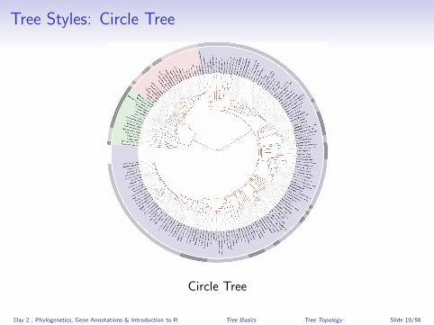
Tree Styles: Circle Tree

Circle Tree


Significance of Branch Lengths in Cladograms, Phylogramsand Ultrametric Trees


Fullyresolved


multifurcation

Species B

Species A

Orthologues


Duplications

= internal node

= external node

= internal branch

= external branch

1 2 3 4 1 2 3 4

=

Taxon A

Taxon B

Taxon C

Taxon D

Taxon A

Taxon B

Taxon C

Taxon D5

4

1

11

1

Taxon A

Taxon B

Taxon C

Taxon D

0510152025





[Million Years]


Rotating Branches in Phylogenetic Trees


Fullyresolved


multifurcation

Species B

Species A

Orthologues


Duplications

= internal node

= external node

= internal branch

= external branch

1 2 3 4 1 2 3 4

=Figure 5: Branch Rotations

Rotations of internal nodes yield exactly the same tree.


Rooting Trees

There are five possibilities to root the unrooted tree on the top left.

Trees rooted on branches c and d are not shown.


OutlineIntroduction

Phylogenetics





References

Day 2 , Phylogenetics, Gene Annotations & Introduction to R Tree Basics Counting Trees Slide 14/56

Number of Unrooted and Rooted Trees

The number of possible trees grows more than exponentially as thenumber of taxa n increases:

N unrooted trees =(2n − 5)!

2n−3(n − 3)!= (2n − 5)!! (1)

N rooted trees =(2n − 3)!

2n−2(n − 2)!= (2n − 3)!! (2)

n = number of leaves (taxa)N = number of possible trees

Example

n N Unrooted Trees N Rooted Trees

3 1 34 3 155 15 1057 954 10,395

10 2,027,025 34,459,425

Day 2 , Phylogenetics, Gene Annotations & Introduction to R Tree Basics Counting Trees Slide 15/56

OutlineIntroduction

Phylogenetics





References

Day 2 , Phylogenetics, Gene Annotations & Introduction to R Tree Basics Tree Rooting Methods Slide 16/56

Methods for Rooting Phylogenetic Trees

Outgroup Method

Rooting by including one or more outgroup taxa/sequences.

Gene Duplication

Paralogous gene duplication predating the common ancestorof a clade are used.

Midpoint Rooting

Tree is rooted by midpoint between the two most distantbranches.


Rooting by Outgroup

Rooting is accomplished by including one or more outgroup(taxa/sequences) that differ from all ingroup members morethan all the ingroup members among each other.

The main assumption of this method is that outgroup taxafall outside of the ingroup.


Rooting with Duplicated Genes

The root is placed between paralogous gene populations.

Gene Copies A

Gene Copies B


Midpoint Rooting

Choose the midpoint between the two most distant branches.

Midpoint rooting assumes that the rate of evolution is thesame on the longest branches of the tree.


OutlineIntroduction

Phylogenetics





References

Day 2 , Phylogenetics, Gene Annotations & Introduction to R Tree Basics Inferring Trees from Distances Slide 21/56

Transforming Characters to Distances

DNA Alignment

G1 TTATTAAG2 AATTTAAG3 AAAAATAG4 AAAAAAT

Distance Matrix

G1 G2 G3 G4

G1 0.43 0.71 0.71G2 3 0.57 0.57G3 5 4 0.29G4 5 4 2

Absolute distances in bottom triangle and uncorrected relative distances in top triangle.

Day 2 , Phylogenetics, Gene Annotations & Introduction to R Tree Basics Inferring Trees from Distances Slide 22/56

OutlineIntroduction

Phylogenetics





References

Day 2 , Phylogenetics, Gene Annotations & Introduction to R Tree Building Methods Slide 23/56

Desirable Features of Tree Building Methods

Consistency: will the method converge on the correct solutiongiven enough data?

Efficiency: how fast is the method?

Robustness: will minor violations of the assumptions result inpoor estimates of phylogeny?

Day 2 , Phylogenetics, Gene Annotations & Introduction to R Tree Building Methods Slide 24/56

OutlineIntroduction

Phylogenetics





References

Day 2 , Phylogenetics, Gene Annotations & Introduction to R Tree Building Methods Clustering Methods Slide 25/56

Clustering Methods

Algorithmic methods in which the algorithm itself defines thetree selection criterion.

No optimality criteria applied.

Advantage: tend to be very fast (efficient) computations thatproduce singular trees.

Disadvantages:

Do not allow evaluation of competing hypotheses.No objective function (e.g. likelihood, number of steps) is usedto compare different trees to each other, even if numerousother trees could explain the data equally well.

Examples that construct trees from distances:

UPGMANeighbor joining (NJ)


UPGMA

UPGMA stands for unweighted pair group method usingarithmetic averages [Sokal & Michener 1958].

Clusters taxa (sequences) agglomeratively and creates at thesame time a hierarchical tree.

The branch (edge) lengths and node positions are determinedby the average distance between clusters.

There are variants of UPGMA that define the distancebetween clusters (linkage method) as the minimum ormaximum of the distances between clusters, rather than theaverage.

The average linkage seems to have the best performancerecords.


UPGMA Algorithm

Initialization

Assign each sequence to its own cluster.

Iteration

Determine the clusters with the smallest distance (d). If thereare several equidistant choices than pick one randomly.

Join these closet clusters to a new (larger) cluster.

Place a node for new cluster at the height corresponding tohalf of the distance between the joined clusters.

Update distances by computing the distance of the newcluster to all other clusters.

Termination

When only two clusters remain place the root at the heightcorresponding to half of their distance.


Illustration of UPGMA Algorithm


Fullyresolved


multifurcation

Species B

Species A

Orthologues


Duplications

= internal node

= external node

= internal branch

= external branch

1 2 3 4 1 2 3 4

=

Taxon A

Taxon B

Taxon C

Taxon D

Taxon A

Taxon B

Taxon C

Taxon D5

4

1

11

1

Taxon A

Taxon B

Taxon C

Taxon D

0510152025





[Million Years]

A B C DA

B

C

-

((A:0.5, B:0.5):0.1,(C:0.5,D:0.5):0.1);

Slanted style

Rectangularstyle

Newick format:

A

B

D

C

D


A

B

C

D

A B C D

e

a

b

c

d

Root:

e

e

A B C D

a

B A C D

b

Root: a

Root: b

Outgroup

Ingroup

A

B

C

D

A

B

C

D

Cladogram

A

B

C

D5

4

1

11

1

Phylogram

Midpoint Rooting

10

7

6

A

B

C

A B

6 6

4

A

B

C

1

1

1

1

A

B

C

1

6

1

1

A

B

C

1

1

1

1

A

B

C

1

6

1

1

Tree A Tree B

A

B

C

D

0.1

0.20.1

0.3

0.4

1 2 54

67

1 2

4

5

3

1/2 d45

1 2

6

1 2

4

5

3

1/2 d12

1 2 5 34

67

8

91 2

4

5

31/2 d68

3-4. Iteration

2. Iteration

1. Iteration


Limitations of UPGMA Algorithm

The edge lengths of an UPGMA tree correspond roughly to the timesmeasured by a molecular clock with constant rate.

The method assumes that the divergence of sequences occurs at allpoints in the tree with a constant rate and the distances are additive.

If the molecular clock assumption applies to a given distance matrix, thenUPGMA constructs the tree correctly.

However, if this assumption does not apply to the underlying distancematrix, then UPGMA may construct the tree incorrectly.

Example Fig 6: correct tree on the left and incorrect UPGMA tree on theright:


Fullyresolved


multifurcation

Species B

Species A

Orthologues


Duplications

= internal node

= external node

= internal branch

= external branch

1 2 3 4 1 2 3 4

=

Taxon A

Taxon B

Taxon C

Taxon D

Taxon A

Taxon B

Taxon C

Taxon D5

4

1

11

1

Taxon A

Taxon B

Taxon C

Taxon D

0510152025





[Million Years]

A B C DA

B

C

-

((A:0.5, B:0.5):0.1,(C:0.5,D:0.5):0.1);

Slanted style

Rectangularstyle

Newick format:

A

B

D

C

D


A

B

C

D

A B C D

e

a

b

c

d

Root:

e

e

A B C D

a

B A C D

b

Root: a

Root: b

Outgroup

Ingroup

A

B

C

D

A

B

C

D

Cladogram

A

B

C

D5

4

1

11

1

Phylogram

Midpoint Rooting

10

7

6

A

B

C

A B

6 6

4

A

B

C

1

1

1

1

A

B

C

1

6

1

1

A

B

C

1

1

1

1

A

B

C

1

6

1

1

Tree A Tree B

A

B

C

D

0.1

0.20.1

0.3

0.4

1 2 54

67

1 2

4

5

3

1/2 d45

1 2

6

1 2

4

5

3

1/2 d12

1 2 5 34

67

8

91 2

4

5

31/2 d68

3-4. Iteration

2. Iteration

1. Iteration

A

C

B

D A

C

B

D

Solution: test if the distance matrix is ultrametric, where in any triplet ofdistances one pair must be equal and the remaining one is the smallest.


Neighbor-Joining Method

If the molecular clock property fails for a given data set, but additivityholds, then the neighbor-joining method can construct a correct tree.

To overcome the problem that neighboring leaves can be more distant toeach other than to non-neighboring leaves (see Fig 6), one can calculatethe rate corrected distances Dij by subtracting from dij the averageddistances to all other leaves:

Dij = dij − (ri + rj), where ri =1

|L| − 2

∑k∈L

dik (3)

|L| is the size of the leaf set L.

Consequence: i and j are neighboring leaves if their Dij is minimal!


Example: Rate Corrected Distance Matrix

Distance Matrix

A B C D

A 0.3 0.7 0.4B -1.2 0.8 0.5C -1.0 -1.0 0.5D -1.0 -1.0 -1.2

Upper right triangle: original distance values.Lower left triangle: rate corrected distances calculated by eq 3 as:

rA = (0.3 + 0.7 + 0.4)/2 = 0.7rB = (0.3 + 0.8 + 0.5)/2 = 0.8rC = (0.7 + 0.8 + 0.5)/2 = 1.0

...DAB = 0.3− 0.7− 0.8 = −1.2DAC = 0.7− 0.7− 1.0 = −1.0

...


Main Differences Between UPGMA and Neighbor-Joining

UPGMA

1 Assumes additivity and ultrametricity.

2 Does not use rate corrected distances values for tree construction.

3 Results in a rooted tree with branch pairs reflecting the distanceinformation.

4 Tree type: cladogram.

5 May fail to generate the correct tree from distance values that violate theultrametricity rule.

Neighbor-Joining

1 Assumes additivity, but not ultrametricity.

2 Uses rate corrected distances values for tree construction.

3 Results in an unrooted tree with the branch lengths reflecting thedistance information.

4 Tree type (after rooting): phylogram or cladogram.

5 Generates correct tree from distance values that may violate theultrametricity rule.


OutlineIntroduction

Phylogenetics





References

Day 2 , Phylogenetics, Gene Annotations & Introduction to R Tree Building Methods Parsimony Methods Slide 34/56

Parsimony

Basic principle: find the tree that explains the observedsequences with the minimal number of substitutions.

Instead of building a tree, like with distance methods,parsimony assigns a cost to a given tree.

This requires searching through all possible trees or a subsetof trees that contains the best or close to best tree topology.

Parsimony algorithms consist of two major steps:1 Computation of the cost for a given tree.2 Search for the tree with minimum cost.


Example: Computing the Cost of a Given Tree

Given a multiple alignment and a tree topology, one can count thenumber of substitution needed for each tree.

The following figure shows two possible trees for the alignment on theleft. Trees differ in the order the sequences are assigned to the leaves.

Hypothetical sequences have been assigned to the ancestral nodes thatminimize the number of substitution needed in the entire tree.


Fullyresolved


multifurcation

Species B

Species A

Orthologues


Duplications

= internal node

= external node

= internal branch

= external branch

1 2 3 4 1 2 3 4

=

Taxon A

Taxon B

Taxon C

Taxon D

Taxon A

Taxon B

Taxon C

Taxon D5

4

1

11

1

Taxon A

Taxon B

Taxon C

Taxon D

0510152025





[Million Years]

A B C DA

B

C

-

((A:0.5, B:0.5):0.1,(C:0.5,D:0.5):0.1);

Slanted style

Rectangularstyle

Newick format:

A

B

D

C

D


A

B

C

D

A B C D

e

a

b

c

d

Root:

e

e

A B C D

a

B A C D

b

Root: a

Root: b

Outgroup

Ingroup

A

B

C

D

A

B

C

D

Cladogram

A

B

C

D5

4

1

11

1

Phylogram

Midpoint Rooting

10

7

6

A

B

C

A B

6 6

4

A

B

C

1

1

1

1

A

B

C

1

6

1

1

A

B

C

1

1

1

1

A

B

C

1

6

1

1

Tree A Tree B

A

B

C

D

0.1

0.20.1

0.3

0.4

1 2 54

67

1 2

4

5

3

1/2 d45

1 2

6

1 2

4

5

3

1/2 d12

1 2 5 34

67

8

91 2

4

5

31/2 d68

3-4. Iteration

2. Iteration

1. Iteration

A

C

B

D A

C

B

D

AAG AAA GGA AGA

AAA AGA

AAA

1 1

1

AAG AGA AAA GGA

AAA AAA

AAA

1 21

��

Alignment Two Possible Parsimony Trees

The tree on the left is more parsimonious than the one on the rightbecause it requires only 3 instead of 4 changes.

As shown here, parsimony treats each site independently and then sumsup the substitutions needed for all sites.


Tree Search Methods

Several tree search methods can be considered:1 Exhaustive Searches: All trees are evaluated only possible for

trees with less than 20 taxa.2 Heuristic Searches: Not guaranteed to find the best tree (e.g.

random branch changes and re-scoring of tree).3 Branch and bound algorithm which does not evaluate all trees,

but guarantees to find the best tree.4 Many other approaches.

Branch and bound algorithm

It exploits the idea that the cost (number of substitutions) of asubtree can only increase by adding an extra edge.It systematically builds trees with increasing numbers of leavesand abandons avenues of tree building whenever an incompletetree exceeds the smallest cost of a complete tree.


OutlineIntroduction

Phylogenetics





References

Day 2 , Phylogenetics, Gene Annotations & Introduction to R Quality Assessment by Resampling Slide 38/56

OutlineIntroduction

Phylogenetics





References

Day 2 , Phylogenetics, Gene Annotations & Introduction to R Quality Assessment by Resampling Bootstrap Slide 39/56

Assessing the Reliability of Tree Branches

Nonparametric resampling methods are often used to estimatethe variance associated with a statistic when the underlyingsampling distribution for a statistic is either unknown ordifficult to derive analytically.

Resampling methods include the bootstrap and the jackknife,both of which operate by repeatedly resampling data from theoriginal data set to estimate the variance of the samplingdistribution.

Although both methods have been used for evaluating thereliability of branches, the bootstrap method is morecommonly applied.


Bootstrap Resampling

Data points are randomly resampled from the original dataset, with replacement, until new data sets with the originalnumber of observations are obtained.

Statistic of interest (e.g. a tree) is computed for eachreplicated data set.

Agreement among the resulting trees is summarized with amajority-rule consensus tree (agreement > 50%).

A bootstrap proportion (BP) is the frequency of occurrence ofa clade (for all replicated data sets) and is a measure ofsupport for a group.


Example: Bootstrapping

Original matrix (alignment) Resampled matrix (alignment)

Majority rule tree with bootstrap proportions (BP) at branch nodes.


Phylogenetics Software (Selection!)

PAUP: complex phylogenetic tool collection (partiallycommercial)

PHYLIP: complex phylogenetic tool collection (free)

MrBayes: popular package for Bayesian inference ofphylogenies.

PAML: many utilities for dealing with different evolutionaryrates.

Many more: see for instance this Link Collection.


http://paup.csit.fsu.edu/

http://evolution.genetics.washington.edu/phylip.html

http://mrbayes.csit.fsu.edu/

http://abacus.gene.ucl.ac.uk/software/paml.html

http://wiki.debian.org/DebianSequenceAnalysis

OutlineIntroduction

Phylogenetics





References

Day 2 , Phylogenetics, Gene Annotations & Introduction to R Functional Gene Annotation Systems Slide 44/56

Overview of Genome Annotation Process

Sequence Assembly

NNN NNN

Chromosome

Scaffolds

Contigs

ShotgunSequences

Assemblyby Alignment

Contig Sequences

AdditionalData

FinishingSteps

Genomic Library

Sequencing

Genome AnnotationAssembled Genome

⇓Gene Finding

⇓Functional Gene Annotation

Day 2 , Phylogenetics, Gene Annotations & Introduction to R Functional Gene Annotation Systems Slide 45/56

OutlineIntroduction

Phylogenetics





References

Day 2 , Phylogenetics, Gene Annotations & Introduction to R Functional Gene Annotation Systems Gene Ontologies Slide 46/56

What Are Ontologies?

Problem: there are no consistent naming conventions for geneand protein functions. This limits the information content ofthe provided annotations, because they are often not ’machinereadable’.

Solution: controlled vocabulary system developed andmaintained by Gene Ontology (GO) Consortium.

Ontologies are a machine interpretable representation of thedifferent components and features of a system (e.g.organism).

The Gene Ontology (GO) annotation systems consists of twomain components:

A dictionary of controlled functional terms.A graph (tree) system represents the relationships among theterms.

Result: a unified functional annotation language that connectsdifferent gene annotation databases.


Database Unification by Gene Ontologies


How Are Gene Ontologies Organized?

Gene Ontologies (GO) are an annotation system thatdescribes functions of genes and their products.

GO consists of three ontologies:

1. Molecular Function (MF): molecular activity/task of genesExamples: carbohydrate binding and ATPase activity

2. Biological Process (BP): broader biological functionExamples: involved in mitosis or purine metabolism,accomplished by ordered assemblies of molecular functions

3. Cellular Component (CC): subcellular location or componentof complexExamples: nucleus, mitochondria or part of RNA polymerase IIholoenzyme


GO Term Relationships are Organized in three DAGs

The ontologies are structured as three directed acyclic graphs(DAGs):

1. DAG for molecular function (MF) terms2. DAG for biological process (BP) terms3. DAG for cellular component (CC) terms

DAGs are similar to hierarchical trees, but a child term canhave multiple parent terms. For example, the biologicalprocess term hexose biosynthesis has two parents, hexosemetabolism and monosaccharide biosynthesis.


DAG Example


Evidence Codes

The supporting data type for GO annotations can be tracked bytheir evidence codes. The current set of evidence codes are:

IDA: Inferred from direct assay

IPI: Inferred from physical interaction

IMP: Inferred from mutant phenotype

IGI: Inferred from genetic interaction

IEP: Inferred from expression pattern

IEA: Inferred from electronic annotation

ISS: Inferred from sequence or structural similarity

TAS: Traceable author statement

NAS: Non-traceable author statement

IC: Inferred by curator

RCA: Reviewed Computational Analysis

ND: no data available


Annotating Genes with GO


OutlineIntroduction

Phylogenetics





References

Day 2 , Phylogenetics, Gene Annotations & Introduction to R Functional Gene Annotation Systems Pathway Annotation Systems Slide 54/56

Pathway Annotation Systems

Pathway annotation systems assign gene products to pathwaymaps.

KEGG (Kyoto Encyclopedia of Genes and Genomes): pathwaydatabase for all organisms.Reactome: general pathway database.EcoCyc: pathway database for bacteria.AraCyc: pathway database for Arabidopsis.Many more...

Advantages over GO: simpler data structure, less duplications.

Disadvantages: low genome coverage (∼30%), contains onlymolecular information content.

Day 2 , Phylogenetics, Gene Annotations & Introduction to R Functional Gene Annotation Systems Pathway Annotation Systems Slide 55/56

OutlineIntroduction

Phylogenetics





References

Day 2 , Phylogenetics, Gene Annotations & Introduction to R References Slide 56/56

References and Books

Pevsner, J (2009) Bioinformatics and Functional Genomics.

Felsenstein J (2004) Inferring Phylogenies. Sinauer Associates, Inc, MA.Pages 1-664.

Fitch (1971) Toward defining the course of evolution: minimum changefor a specified tree topology. Systematic Zoology 20: 406-416.

Iwabe N, Kuma K, Hasegawa M, Osawa S, Miyata T (1989) Evolutionaryrelationship of archaebacteria, eubacteria, and eukaryotes inferred fromphylogenetic trees of duplicated genes. Proc Natl Acad Sci U S A 86:9355-9359.URL http://www.hubmed.org/display.cgi?uids=2531898

Sokal RR and Michener CD (1958) A statistical method for evaluatingsystematic relationships. University of Kansas Scientific Bulletin 28:1409-1438.

Day 2 , Phylogenetics, Gene Annotations & Introduction to R References Slide 56/56

http://www.hubmed.org/display.cgi?uids=2531898

bioinformatics workshop -...

Documents