bioinformatics toolbox - cda.psych.uiuc.educda.psych.uiuc.edu/matlab_pdf/bioinfo_ug.pdf · 1...
TRANSCRIPT

Bioinformatics ToolboxFor Use with MATLAB®
Computation
Visualization
Programming
User’s GuideVersion 1

How to Contact The MathWorks:
www.mathworks.com Webcomp.soft-sys.matlab Newsgroup
[email protected] Technical [email protected] Product enhancement [email protected] Bug [email protected] Documentation error [email protected] Order status, license renewals, [email protected] Sales, pricing, and general information
508-647-7000 Phone
508-647-7001 Fax
The MathWorks, Inc. Mail3 Apple Hill DriveNatick, MA 01760-2098
For contact information about worldwide offices, see the MathWorks Web site.
Bioinformatics Toolbox User’s Guide© COPYRIGHT 2003 - 2004 by The MathWorks, Inc.The software described in this document is furnished under a license agreement. The software maybe used or copied only under the terms of the license agreement. No part of this manual may bephotocopied or reproduced in any form without prior written consent from The MathWorks, Inc.
FEDERAL ACQUISITION: This provision applies to all acquisitions of the Program andDocumentation by, for, or through the federal government of the United States. By acceptingdelivery of the Program or Documentation, the government hereby agrees that this software ordocumentation qualifies as commercial computer software or commercial computer softwaredocumentation as such terms are used or defined in FAR 12.212, DFARS Part 227.72, and DFARS252.227-7014. Accordingly, the terms and conditions of this Agreement and only those rightsspecified in this Agreement, shall pertain to and govern the use, modification, reproduction,release, performance, display, and disclosure of the Program and Documentation by the federalgovernment (or other entity acquiring for or through the federal government) and shall supersedeany conflicting contractual terms or conditions. If this License fails to meet the government’s needsor is inconsistent in any respect with federal procurement law, the government agrees to return theProgram and Documentation, unused, to The MathWorks, Inc.
MATLAB, Simulink, Stateflow, Handle Graphics, and Real-Time Workshop are registeredtrademarks, and TargetBox is a trademark of The MathWorks, Inc.
Other product or brand names are trademarks or registered trademarks of their respective holders.
Printing History:September 2003 Online only New for Version 1.0 (Release 13SP1+)June 2004 Online only Updated for Version 1.1 (Release 14)

Contents
Getting Started
1What Is the Bioinformatics Toolbox? . . . . . . . . . . . . . . . . . . 1-2
Expected User . . . . . . . . . . . . . . . . . . . . . . . . . . . . . . . . . . . . . . 1-3
Installation . . . . . . . . . . . . . . . . . . . . . . . . . . . . . . . . . . . . . . . . . 1-5Required Software . . . . . . . . . . . . . . . . . . . . . . . . . . . . . . . . . . . 1-5Additional Software . . . . . . . . . . . . . . . . . . . . . . . . . . . . . . . . . 1-5
Features and Functions . . . . . . . . . . . . . . . . . . . . . . . . . . . . . . 1-7Data Formats and Databases . . . . . . . . . . . . . . . . . . . . . . . . . . 1-7Sequence Alignments . . . . . . . . . . . . . . . . . . . . . . . . . . . . . . . . 1-9Sequence Utilities and Statistics . . . . . . . . . . . . . . . . . . . . . . 1-9Microarray Analysis . . . . . . . . . . . . . . . . . . . . . . . . . . . . . . . . 1-10Protein Structure Analysis . . . . . . . . . . . . . . . . . . . . . . . . . . . 1-10Phylogenetic Analysis . . . . . . . . . . . . . . . . . . . . . . . . . . . . . . . 1-11Prototype and Development Environment . . . . . . . . . . . . . . 1-12Data Visualization . . . . . . . . . . . . . . . . . . . . . . . . . . . . . . . . . . 1-12Algorithm Sharing and Application
Deployment . . . . . . . . . . . . . . . . . . . . . . . . . . . . . . . . . . . . . 1-12
Sequence Analysis
2Example: Sequence Statistics . . . . . . . . . . . . . . . . . . . . . . . . . 2-2
Determining Nucleotide Content . . . . . . . . . . . . . . . . . . . . . . . 2-2Getting Sequence Information into MATLAB . . . . . . . . . . . . . 2-4Determining Nucleotide Composition . . . . . . . . . . . . . . . . . . . 2-5Determining Codon Composition . . . . . . . . . . . . . . . . . . . . . . . 2-8Open Reading Frames . . . . . . . . . . . . . . . . . . . . . . . . . . . . . . 2-11Amino Acid Conversion and Composition . . . . . . . . . . . . . . . 2-14
Example: Sequence Alignment . . . . . . . . . . . . . . . . . . . . . . . 2-17
i

Finding a Model Organism to Study . . . . . . . . . . . . . . . . . . . 2-17Getting Sequence Information from a Public
Database . . . . . . . . . . . . . . . . . . . . . . . . . . . . . . . . . . . . . . . 2-19Searching a Public Database for Related Genes . . . . . . . . . . 2-21Locating Protein Coding Sequences . . . . . . . . . . . . . . . . . . . . 2-24Comparing Amino Acid Sequences . . . . . . . . . . . . . . . . . . . . . 2-27
Microarray Analysis
3Example: Visualizing Microarray Data . . . . . . . . . . . . . . . . 3-2
Overview of the Mouse Example . . . . . . . . . . . . . . . . . . . . . . . 3-2Exploring the Microarray Data Set . . . . . . . . . . . . . . . . . . . . . 3-3Spatial Images of Microarray Data . . . . . . . . . . . . . . . . . . . . . 3-5Statistics of the Microarrays . . . . . . . . . . . . . . . . . . . . . . . . . 3-15Scatter Plots of Microarray Data . . . . . . . . . . . . . . . . . . . . . . 3-16
Example: Analyzing Gene ExpressionProfiles . . . . . . . . . . . . . . . . . . . . . . . . . . . . . . . . . . . . . . . . . . 3-25Overview of the Yeast Example . . . . . . . . . . . . . . . . . . . . . . . 3-25Exploring the Data Set . . . . . . . . . . . . . . . . . . . . . . . . . . . . . . 3-25Filtering Genes . . . . . . . . . . . . . . . . . . . . . . . . . . . . . . . . . . . . 3-29Clustering Genes . . . . . . . . . . . . . . . . . . . . . . . . . . . . . . . . . . . 3-32Principal Component Analysis . . . . . . . . . . . . . . . . . . . . . . . . 3-36
Phylogenetic Analysis
4Example: Building a Phylogenetic Tree . . . . . . . . . . . . . . . . 4-2
Overview for the Primate Example . . . . . . . . . . . . . . . . . . . . . 4-2Searching NCBI for Phylogenetic Data . . . . . . . . . . . . . . . . . . 4-4Creating a Phylogenetic Tree for Five Species . . . . . . . . . . . . 4-6Creating a Phylogenetic Tree for Twelve Species . . . . . . . . . . 4-8Exploring the Phylogenetic Tree . . . . . . . . . . . . . . . . . . . . . . 4-10
Phylogenetic Tree Tool Reference . . . . . . . . . . . . . . . . . . . . 4-14
ii Contents

Opening the Phytreetool GUI . . . . . . . . . . . . . . . . . . . . . . . . . 4-14File Menu . . . . . . . . . . . . . . . . . . . . . . . . . . . . . . . . . . . . . . . . . 4-16Tools Menu . . . . . . . . . . . . . . . . . . . . . . . . . . . . . . . . . . . . . . . . 4-24Windows Menu . . . . . . . . . . . . . . . . . . . . . . . . . . . . . . . . . . . . 4-32Help Menu . . . . . . . . . . . . . . . . . . . . . . . . . . . . . . . . . . . . . . . . 4-32
Functions – Categorical List
5Data Formats and Databases . . . . . . . . . . . . . . . . . . . . . . . . . 5-2
Sequence Conversion . . . . . . . . . . . . . . . . . . . . . . . . . . . . . . . . 5-4
Sequence Statistics . . . . . . . . . . . . . . . . . . . . . . . . . . . . . . . . . . 5-5
Sequence Utilities . . . . . . . . . . . . . . . . . . . . . . . . . . . . . . . . . . . 5-6
Pairwise Sequence Alignment . . . . . . . . . . . . . . . . . . . . . . . . 5-7
Protein Analysis . . . . . . . . . . . . . . . . . . . . . . . . . . . . . . . . . . . . . 5-8
Trace Tools . . . . . . . . . . . . . . . . . . . . . . . . . . . . . . . . . . . . . . . . . . 5-9
Profile Hidden Markov Models . . . . . . . . . . . . . . . . . . . . . . . 5-10
Microarray File Formats . . . . . . . . . . . . . . . . . . . . . . . . . . . . 5-11
Microarray Visualization . . . . . . . . . . . . . . . . . . . . . . . . . . . . 5-12
Microarray Normalization and Filtering . . . . . . . . . . . . . . 5-13
Scoring Matrices . . . . . . . . . . . . . . . . . . . . . . . . . . . . . . . . . . . 5-14
Phylogenetic Tree Tools . . . . . . . . . . . . . . . . . . . . . . . . . . . . . 5-15
iii

Phylogenetic Tree Methods . . . . . . . . . . . . . . . . . . . . . . . . . . 5-16
Tutorials, Demos, and Examples . . . . . . . . . . . . . . . . . . . . . 5-17
Functions — Alphabetical List
6
Examples
ASequence Analysis . . . . . . . . . . . . . . . . . . . . . . . . . . . . . . . . . . . A-2
Microarray Analysis . . . . . . . . . . . . . . . . . . . . . . . . . . . . . . . . . A-3
Phylogenetic Analysis . . . . . . . . . . . . . . . . . . . . . . . . . . . . . . . . A-4
Index
iv Contents

1
Getting Started
This chapter is an overview of the functions and features in the BioinformaticsToolbox. An introduction to these features will help you to develop aconceptual model for working with the toolbox and your biological data.
“What Is the BioinformaticsToolbox?” (p. 1-2)
Description of this toolbox and theintended user
“Installation” (p. 1-5) Required software and additional softwarefor developing advanced algorithms
“Features and Functions” (p.1-7)
Functions grouped into categories thatsupport bioinformatic tasks

1 Getting Started
What Is the Bioinformatics Toolbox?The Bioinformatics Toolbox extends MATLAB® to provide an integratedsoftware environment for genome and proteome analysis. Together,MATLAB and the Bioinformatics Toolbox give scientists and engineers aset of computational tools to solve problems and build applications in drugdiscovery, genetic engineering, and biological research.
You can use the basic bioinformatic functions provided with this toolbox tocreate more complex algorithms and applications. These robust and welltested functions are the functions that you would otherwise have to createyourself.
• Connecting to Web accessible databases
• Reading and converting between multiple data formats
• Determining statistical characteristics of data
• Manipulating and aligning sequences
• Modeling patterns in biological sequences using Hidden Markov Model(HMM) profiles
• Reading, normalizing, and visualizing microarray data
• Creating and manipulating phylogenetic tree data
• Interfacing with other bioinformatic software (BioPearl and BioJava)
The field of bioinformatics is rapidly growing and will become increasinglyimportant as biology becomes a more analytical science. The BioinformaticsToolbox provides an open environment that you can customize for developmentand deployment of the analytical tools you and scientists will need.
Prototype and develop algorithms — Prototype new ideas in an open andextendable environment. Develop algorithms using efficient string processingand statistical functions, view the source code for existing functions, and usethe code as a template for improving or creating your own functions. See“Prototype and Development Environment” on page 1-12.
1-2
What Is the Bioinformatics Toolbox?
Visualize data — Visualize sequence alignments, gene expression data,phylogenetic trees, and protein structure analyses. See “Data Visualization”on page 1-12.
Share and deploy applications — Use an interactive GUI builder todevelop a custom graphical front end for your data analysis programs. Createstand-alone applications that run separate from MATLAB. See “AlgorithmSharing and Application Deployment” on page 1-12.
1-3

1 Getting Started
Expected UserThe Bioinformatics Toolbox is for computational biologists and researchscientists who need to develop new or implement published algorithms,visualize results, and create stand-alone applications.
• Industry/Professional — Increasingly, drug discovery methods are beingsupported by engineering practice. This toolbox supports tool builderswho want to create applications for the biotechnology and pharmaceuticalindustry.
• Education/Student — This toolbox is well suited for learning and teachinggenome and proteome analysis techniques. Educators and students canconcentrate on bioinformatic algorithms instead of programming basicfunctions such as reading and writing to files.
While the toolbox includes many bioinformatics functions, it is not intendedto be a complete set of tools for scientists to analyze their biological data.However, MATLAB is the ideal environment for you to rapidly design andprototype the tools you will need.
1-4

Installation
InstallationYou don’t need to do anything special when installing the BioinformaticsToolbox. Install the toolbox from a CD or Web release using The MathWorksinstaller.
• “Required Software” on page 1-5 — List of MathWorks products you needto purchase with the Bioinformatics Toolbox
• “Additional Software” on page 1-5 — List of toolboxes from The MathWorksfor advanced algorithm development
Required SoftwareThe Bioinformatics Toolbox requires the following products from theMathWorks to be installed on your computer:
MATLAB Provides a command-line interface andintegrated software environment for theBioinformatics Toolbox.Version 1.1.1 of theBioinformatics Toolbox requires MATLABVersion 7.0.1 on the Release 14 CD.
Statistics Toolbox Provides basic statistics and probabilityfunctions that the functions in theBioinformatics Toolbox use.Version 1.1.1of the Bioinformatics Toolbox requires theStatistics Toolbox Version 5.0.1 on the Release14 CD or downloaded from the Web.
Additional SoftwareMATLAB and the Bioinformatics Toolbox provide an open and extensiblesoftware environment. In this environment you can interactively exploreideas, prototype new algorithms, and develop complete solutions to problemsin bioinformatics. The MATLAB language facilitates the use of computation,visualization, prototyping, and deployment.
Using the Bioinformatics Toolbox in combination with other MATLABtoolboxes and products, will allow your to solve multidisciplinary problems.
1-5

1 Getting Started
Signal Processing Toolbox Process signal data from bioanalyticalinstrumentation. Examples includeacquisition of fluorescence data forDNA sequence analyzers, fluorescencedata for microarray scanners, and massspectrometric data from protein analyses.
Image Processing Toolbox Create complex and custom imageprocessing algorithms for data frommicroarray scanners.
Optimization Toolbox Use nonlinear optimization for predictingthe secondary structure of proteinsand the structure of other biologicalmacromolecules.
Neural Network Toolbox Use neural networks to solve problemswhere algorithms are not available. Forexample, you can train neural networksfor pattern recognition using large sets ofsequence data.
Database Toolbox Create your own in-house databases forsequence data with custom annotations.
MATLAB Compiler Create stand-alone applications fromMATLAB GUI applications, and createdynamic link libraries from MATLABfunctions for use with any programmingenvironment.
MATLAB® Builder for COM Create COM objects to use with anyCOM-based programming environment.
MATLAB® Builder for Excel Create Excel add-in functions fromMATLAB functions to use with Excelspreadsheets.
1-6
Features and Functions
Features and FunctionsThe Bioinformatics Toolbox includes many functions to help you with genomeand proteome analysis. Most functions are implemented in M-Code (theMATLAB programming language) with the source available for you to view.This open environment lets you explore and customize the existing toolboxalgorithms or develop your own.
• “Data Formats and Databases” on page 1-7 — Access online databases,copy data into the MATLAB workspace, and read and write to files withstandard bioinformatic formats.
• “Sequence Alignments” on page 1-9 — Compare nucleotide or amino acidsequences using pairwise and multiple sequence alignment functions.
• “Sequence Utilities and Statistics ” on page 1-9 — Manipulate sequencesand determine physical, chemical, and biological characteristics.
• “Microarray Analysis” on page 1-10 — Read, filter, normalize, and visualizemicroarray data.
• “Protein Structure Analysis” on page 1-10 — Determine proteincharacteristics and simulate enzyme cleavage reactions.
• “Phylogenetic Analysis” on page 1-11 — Explore phylogenetic data withfunctions and a GUI to draw phylograms (trees)
• “Prototype and Development Environment” on page 1-12 — Create newalgorithms, try new ideas, and compare alternatives.
• “Data Visualization” on page 1-12 — Visually compare pairwise andmultiply aligned sequences, gene expression data from microarrays, andplot nucleic acid and protein characteristics.
• “Algorithm Sharing and Application Deployment” on page 1-12 — CreateGUIs and stand-alone applications.
Data Formats and DatabasesThe Bioinformatics Toolbox supports access to many of the databases on theWeb and other online sources. It also reads many common genome file formatsso that you do not have to write and maintain your own file readers.
1-7

1 Getting Started
Web-based databases — You can directly access public databases on theWeb and copy sequence and gene expression information into MATLAB.
Currently supported sequence databases are GenBank (getgenbank), GenPept(getgenpept), European Molecular Biology Laboratory EMBL (getembl),Protein Sequence Database PIR-PSD (getpir), and Protein Data Bank PDB(getpdb). You can also access data from the NCBI Gene Expression Omnibus(GEO) web site by using a single function (getgeodata).
Get multiple aligned sequences (gethmmalignment), hidden Markov modelprofiles (gethmmprof), and phylogenetic tree data (gethmmtree) from thePFAM database.
Raw data — Read and visualize data generated from gene sequencinginstruments in MATLAB (scfread, joinseq, traceplot).
Reading data formats — The toolbox provides a number of functions forreading data from common file formats.
• Sequence data: GenBank (genbankread), GenPept (genpeptread), EMBL(emblread), PIR-PSD (pirread), PDB (pdbread), and FASTA (
fastaread
• Multiply aligned sequences: ClustalW and GCG formats (multialignread).
• Gene expression data from microarrays: Gene Expression Omnibus (GEO)data ( geosoftread), GenePix data (galread, gprread), and SPOT data(sptread), Affymetrix data (affyread)
Note: The function affyread only works on PC supported platforms.
• Hidden Markov Model profiles: PFAM-HMM file (pfamhmmread).
Writing data formats — The functions for getting data from the Web includethe option to save the data to a file. However, there is a function to write datato a file using the FASTA format ( fastawrite).
MATLAB has built-in support for other industry-standard file formatsincluding Microsoft Excel and comma-separated value (CSV) files. Additionalfunctions perform ASCII and low-level binary I/O, allowing you to developcustom functions for working with any data format.
1-8

Features and Functions
Sequence AlignmentsYou can select from a list of analysis methods to perform pairwise or multiplesequence alignment.
Pairwise sequence alignment — The toolbox provides efficient MATLABimplementations of standard algorithms such as the Needleman-Wunsch(nwalign) and Smith-Waterman (swalign) algorithms for pairwise sequencealignment. The toolbox also includes standard scoring matrices such as thePAM and BLOSUM families of matrices (blosum, dayhoff, gonnet, nuc44,pam).
Sequence profile alignment — The toolbox provides efficient MATLABimplementations for profile hidden Markov model algorithms (gethmmprof,gethmmalignment, pfamhmmread, hmmprofalign, hmmprofestimate,hmmprofgenerate, hmmprofmerge, hmmprofstruct, showhmmprof).
Visualizing sequence alignments — Once you have analyzed your data,there are several tools for visualizing your sequence alignments (seqdotplot,showalignment, seqshowwords, seqshoworfs).
Biological codes — Look up the letters or numerical equivalents forcommonly used biological codes (aminolookup, geneticcode, revgeneticcode).
Sequence Utilities and StatisticsYou can manipulate and analyze your sequence to gain a deeper understandingof your data.
Sequence manipulation — The toolbox provides routines for commonoperations such as converting DNA or RNA sequences to amino acid sequencesthat are basic to working with nucleic acid or protein sequences (aa2int,aa2nt, dna2rna, rna2dna, int2aa, int2nt, nt2aa, nt2int, seqcomplement,seqrcomplement, seqreverse).
You can manipulate your sequence by performing an in-silico digestion withrestriction endonucleases (restrict) and proteases (cleave ).
Sequence statistics — You can determine various statistics about asequences (aacount, basecount, codoncount, dimercount, nmercount,ntdensity), search for specific patterns within a sequence (seqshowwords,
1-9

1 Getting Started
seqwordcount), or search for open reading frames (seqshoworfs). In addition,you can create random sequences for test cases (randseq).
Additional functions in MATLAB efficiently handle string operations withregular expressions (regexp, seq2regexp) to look for specific patterns in asequence, and look for possible cleavage sites in a DNA/RNA sequence bysearching for palindromes (palindromes).
Microarray AnalysisMATLAB is widely used for microarray data analysis. However, the standardnormalization and visualization tools that scientists use can be difficult toimplement. The Bioinformatics Toolbox includes these standard functions.
Microarray normalization — The toolbox provides a number of methodsfor normalizing microarray data, such as lowess normalization (malowess),global mean normalization (mameannorm), and median absolute deviation(MAD) normalization (mamadnorm). You can use filtering functions toclean raw data before analysis (geneentropyfilter, genelowvalfilter,generangefilter, genevarfilter), and calculate the range and variance ofvalues (exprprofrange, exprprofvar).
Microarray visualization — The toolbox contains routines for visualizingmicroarray data. These routines include spacial plots of microarray data(maimage, redgreencmap), box plots (maboxplot), loglog plot (maloglog), andintensity-ratio plots (mairplot). You can also view clustered expressionprofiles (clustergram, redgreencmap)
The toolbox accesses statistical routines to perform cluster analysis and tovisualize the results.
MATLAB visualization tools let you view your data through statisticalvisualizations such as dendrograms, classification, and regression trees.
Protein Structure AnalysisYou can use a collection of protein analysis methods to extract informationfrom your data. The toolbox provides functions to calculate various propertiesof a protein sequence such as the atomic composition (atomiccomp) and themolecular weight (molweight). You can cleave a protein with an enzyme
1-10

Features and Functions
(cleave ) and create distance and Ramachandran plots for PDB data(pdbdistplot, ramachandran). The toolbox contains a graphical user interfacefor protein analysis (proteinplot). After analyzing the data, you can createrevealing visualizations of your results.
Phylogenetic AnalysisFunctions for phylogenetic tree building and analysis.
• phytreeread — Read a Newick formatted tree file into the MATLABworkspace and return a phytree object with data from the file. Data in thefile uses the Newick (New Hampshire) format for describing trees.
• phytreewrite — Copy the contents of a phytree object from the MATLABworkspace to a file.
• phytreetool — Interactive GUI that allows you to view, edit, and explorephylogenetic tree data. This GUI allows branch pruning, reordering,renaming, and distance exploring. It can also open or save Newickformatted files.
• seqpdist — Calculate the pairwise distance between biological sequences.
• seqlinkage — Construct a phylogenetic tree from pairwise distances.
MALTLAB object and methods for manipulating phylogenetic tree data.
• phytree — Function to create a phytree object.
• phytree/get — Get property values from a phytree object
• phytree/getbyname — Get node names from a phytree object.
• phytree/pdist — Calculate the patristic distances between pairs of leafnodes.
• phytree/plot — Draw a phylogenetic tree object in a MATLAB figurewindow as a phylogram, cladogram, or radial tree.
• phytree/prune — Remove nodes from a phylogenetic tree.
• phytree/select — Select branches and leaves from a phylogenetic tree usinga specified criteria.
• phytree/view — Opens a phylogenetic tree in a phytreetool window.
1-11

1 Getting Started
Prototype and Development EnvironmentMATLAB is a prototyping and development environment where you cancreate algorithms and easily compare alternatives.
• Integrated environment — Explore biological data in an environmentthat integrates programming and visualization. Create reports and plotswith the built-in functions for math, graphics, and statistics.
• Open environment — Access the source code for the BioinformaticsToolbox functions, The toolbox includes many of the basic bioinformaticsfunctions you will need to use, and it includes prototypes for some of themore advanced functions. Modify these functions to create your owncustom solutions.
• Interactive programming language — Test your ideas by typingfunctions that are interpreted interactively with a language whose basicdata element is an array. The arrays do not require dimensioning and allowyou to solve many technical computing problems,
Using matrixes for sequences or groups of sequences allows you to workefficiently with sequences and not worry about writing loops or otherprogramming controls.
• Programming tools — Use a visual debugger for algorithm developmentand refinement and an algorithm performance profiler to acceleratedevelopment
Data VisualizationIn addition, MATLAB 2D and volume visualization features let you createcustom graphical representations of multidimensional data sets. You can alsocreate montages and overlays, and export finished graphics to a PostScriptimage file or copy directly into Microsoft PowerPoint.
Algorithm Sharing and Application DeploymentThe open MATLAB environment lets you share your analysis solutionswith other MATLAB users, and it includes tools to create custom softwareapplications. With the addition of the MATLAB Compiler, you can createstand-alone applications independent from MATLAB, and with the addition ofthe MATLAB COM Builder, you can create GUIs and stand-alone applicationswithin other programming environments.
1-12

Features and Functions
• Share algorithms with other MATLAB users — You can share dataanalysis algorithms created in the MATLAB language across all MATLABsupported platforms by giving M-files to other MATLAB users, Also, youcan create GUIs within MATLAB using the Graphical User InterfaceDevelopment Environment (GUIDE).
• Deploy MATLAB GUIs — Create a GUI within MATLAB using GUIDE,and then use the MATLAB Compiler to create a stand-alone GUIapplication that runs separate from MATLAB.
• Create dynamic link libraries (DLL) — Use the MATLAB compiler tocreate dynamic link libraries (DLLs) for your functions, and then link theselibraries to other programming environments such as C and C++.
• Create COM objects — Use the MATLAB COM Builder to create COMobjects, and then use a COM compatible programming environment (VisualBasic) to create a stand-alone application.
• Create Excel add-ins — Use the MATLAB Excel Builder to createExcel add-in functions, and then use the add-in functions with Excelspreadsheets.
1-13

1 Getting Started
1-14

2
Sequence Analysis
Sequence analysis is the process you use to find information about a nucleotideor amino acid sequence using computational methods. Common tasks insequence analysis are identifying genes, determining the similarity of twogenes, determining the protein coded by a gene, and determining the functionof a gene by finding a similar gene in another organism with a know function.
“Example: SequenceStatistics” (p. 2-2)
Starting with a DNA sequence, calculatestatistics for the nucleotide content.
“Example: SequenceAlignment” (p. 2-17)
Starting with a DNA sequence for a humangene, locate and verify a corresponding genein a model organism.

2 Sequence Analysis
Example: Sequence StatisticsAfter sequencing a piece of DNA, one of the first tasks is to investigate thenucleotide content in the sequence. Starting with a DNA sequence, thisexample uses sequence statistics functions to determine mono-, di-, andtrinucleotide content, and to locate open reading frames.
• “Determining Nucleotide Content” on page 2-2 — Use the MATLAB Helpbrowser to search the Web for information.
• “Getting Sequence Information into MATLAB” on page 2-4 — Find anucleotide sequence in a public database and read the sequence informationinto MATLAB.
• “Determining Nucleotide Composition” on page 2-5 — Determine themonomers and dimers, and then visualize data in graphs and bar plots.
• “Determining Codon Composition” on page 2-8 — Look at codons for the sixreading frames.
• “Open Reading Frames” on page 2-11 — Locate the open reading framesusing a specific genetic code.
• “Amino Acid Conversion and Composition” on page 2-14 — Extract theprotein-coding sequence from a gene sequence and convert it to the aminoacid sequence for the protein.
Determining Nucleotide ContentIn this example you are interested in studying the human mitochondrialgenome. While many genes that code for mitochondrial proteins are found inthe cell nucleus, the mitochondrial has genes that code for proteins used toproduce energy.
First research information about the human mitochondria and find thenucleotide sequence for the genome. Next, look at the nucleotide content forthe entire sequence. And finally, determine open reading frames and extractspecific gene sequences.
2-2

Example: Sequence Statistics
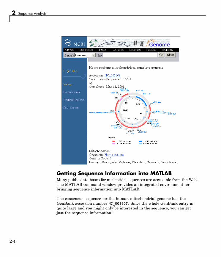
1 Use the MATLAB Help browser to explore the Web. In the MATLABCommand Window, type
web('http://www.ncbi.nlm.nih.gov/')
A separate browser window opens with the home page for the NCBI Website.
2 Search the NCBI Web site for information. For example, to search for thehuman mitochondrion genome, from the Search list, select Genome, and inthe for box, enter mitochondrion homo sapiens.
The NCBI Web search returns a list of links to relevant pages.
3 Select a result page. For example, click the link labeled NC_001807.
The MATLAB Help browser displays the NCBI page for the humanmitochondrial genome.
2-3
2 Sequence Analysis
Getting Sequence Information into MATLABMany public data bases for nucleotide sequences are accessible from the Web.The MATLAB command window provides an integrated environment forbringing sequence information into MATLAB.
The consensus sequence for the human mitochondrial genome has theGenBank accession number NC_001807. Since the whole GenBank entry isquite large and you might only be interested in the sequence, you can getjust the sequence information.
2-4

Example: Sequence Statistics
1 Get sequence information from a Web database.For example, to getsequence information for the human mitochondrial genome, in theMATLAB Command Window, type
mitochondria = getgenbank('NC_001807','SequenceOnly',true);
MATLAB gets the nucleotide sequence from the GenBank database andcreates a character array.
mitochondria =gatcacaggtctatcaccctattaaccactcacgggagctctccatgcatttggtattttcgtctggggggtgtgcacgcgatagcattgcgagacgctggagccggagcaccctatgtcgcagtatctgtctttgattcctgcctcattctattatttatcgcacctacgttcaatattacaggcgaacatacctactaaagt . . .
2 If you don’t have a Web connection, you can load the data from a MAT-fileincluded with the Bioinformatics Toolbox, using the command
load mitochondria
MATLAB loads the sequence mitochondria into the MATLAB workspace.
3 Get information about the sequence. Type
whos mitochondria
MATLAB displays information about the size of the sequence.
Name Size Bytes Classmitochondria 1x16571 33142 char array
Grand total is 16571 elements using 33142 bytes
Determining Nucleotide CompositionSections of a DNA sequence with a high percent of A+T nucleotides usuallyindicates intergenic parts of the sequence, while low A+T and higher G+Cnucleotide percentages indicate possible genes. Many times high CGdinucleotide content is located before a gene.
After you read a sequence into MATLAB, you can use the sequencestatistics functions to determine if your sequence has the characteristics of a
2-5

2 Sequence Analysis
protein-coding region. This procedure uses the human mitochondrial genomeas an example. See “Getting Sequence Information into MATLAB” on page2-4.
1 Plot monomer densities and combined monomer densities in a graph. Inthe MATLAB Command window, type
ntdensity(mitochondria)
This graph shows that the genome is A+T rich.
2 Count the nucleotides using the function basecount.basecount(mitochondria)
A list of nucleotide counts is shown for the 5’-3’ strand.ans =A: 5113C: 5192G: 2180T: 4086
2-6

Example: Sequence Statistics
3 Count the nucleotides in the reverse complement of a sequence using thefunction seqrcomplement.
basecount(seqrcomplement(mitochondria))
As expected, the nucleotide counts on the reverse complement strand arecomplementary to the 5’-3’ strand.
ans =A: 4086C: 2180G: 5192T: 5113
4 Use the function basecount with the chart option to visualize thenucleotide distribution.
basecount(mitochondria,'chart','pie');
MATLAB draws a pie chart in a figure window.
2-7

2 Sequence Analysis
5 Count the dimers in a sequence and display the information in a bar chart.
dimercount(mitochondria,'chart','bar')
MATLAB lists the dimer counts and draws a bar chart.
Determining Codon CompositionTrinucleotides (codon) code for an amino acid, and there are 64 possible codonsin a nucleotide sequence. Knowing the percent of codons in your sequence canbe helpful when you are comparing with tables for expected codon usage.
After you read a sequence into MATLAB, you can analyze the sequence forcodon composition. This procedure uses the human mitochondria genome asan example. See “Getting Sequence Information into MATLAB” on page 2-4.
1 Count codons in a nucleotide sequence. In the MATLAB CommandWindow, type
codoncount(mitochondria)
MATLAB displays the codon counts for the first reading frame.
2-8
Example: Sequence Statistics
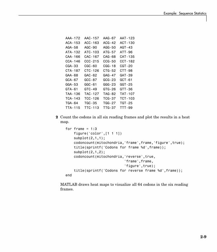
AAA-172 AAC-157 AAG-67 AAT-123ACA-153 ACC-163 ACG-42 ACT-130AGA-58 AGC-90 AGG-50 AGT-43ATA-132 ATC-103 ATG-57 ATT-96CAA-166 CAC-167 CAG-68 CAT-135CCA-146 CCC-215 CCG-50 CCT-182CGA-33 CGC-60 CGG-18 CGT-20CTA-187 CTC-126 CTG-52 CTT-98GAA-68 GAC-62 GAG-47 GAT-39GCA-67 GCC-87 GCG-23 GCT-61GGA-53 GGC-61 GGG-23 GGT-25GTA-61 GTC-49 GTG-26 GTT-36TAA-136 TAC-127 TAG-82 TAT-107TCA-143 TCC-126 TCG-37 TCT-103TGA-64 TGC-35 TGG-27 TGT-25TTA-115 TTC-113 TTG-37 TTT-99
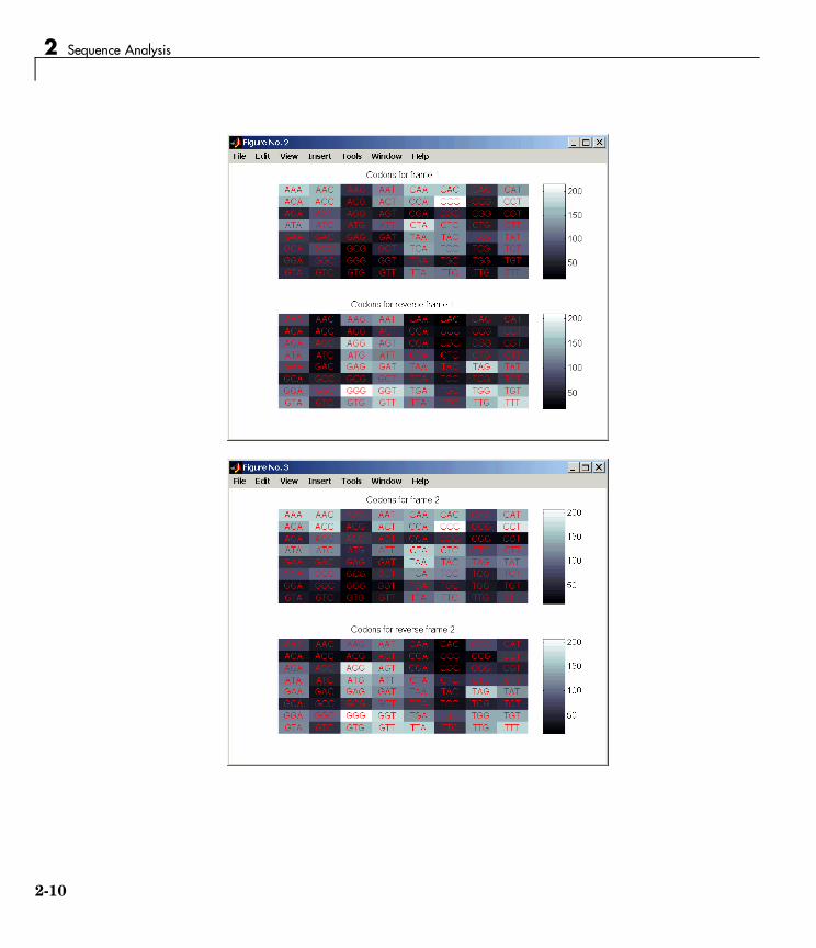
2 Count the codons in all six reading frames and plot the results in a heatmap.
for frame = 1:3figure('color',[1 1 1])subplot(2,1,1);codoncount(mitochondria,'frame',frame,'figure',true);title(sprintf('Codons for frame %d',frame));subplot(2,1,2);codoncount(mitochondria,'reverse',true,
'frame',frame,'figure',true);
title(sprintf('Codons for reverse frame %d',frame));end
MATLAB draws heat maps to visualize all 64 codons in the six readingframes.
2-9
2 Sequence Analysis
2-10

Example: Sequence Statistics
Open Reading FramesDetermining the protein-coding sequence for a eukaryotic gene can be adifficult task because introns (noncoding sections) are mixed with exons.However, prokaryotic genes generally do not have introns and mRNAsequences have the introns removed. Identifying the start and stop codonsfor translation determines the protein-coding section or open reading frame(ORF) in a sequence. Once you know the ORF for a gene or mRNA, you cantranslate a nucleotide sequence to its corresponding amino acid sequence.
After you read a sequence into MATLAB, you can analyze the sequence foropen reading frames. This procedure uses the human mitochondria genome asan example. See “Getting Sequence Information into MATLAB” on page 2-4.
1 Display open reading frames (ORFs) in a nucleotide sequence. In theMATLAB Command window, type
showorfs(mitochondria);
If you compare this output to the genes shown on the NCBI page forNC_001807, there are fewer genes than expected. This is because vertebrate
2-11

2 Sequence Analysis
mitochondria use a genetic code slightly different from the standard geneticcode. For a table of genetic codes, see Genetic Code on page 6-4.
2 Display ORFs using the Vertebrate Mitochondrial code.
orfs= seqshoworfs(mitochondria,'GeneticCode','Vertebrate Mitochondrial','alternativestart',true);
Notice that there are now two large ORFs on the first reading frame. Onestarts at position 4471 and the other starts at 5905. These correspond tothe genes ND2 (NADH dehydrogenase subunit 2 [Homo sapiens] ) andCOX1 (cytochrome c oxidase subunit I) genes.
3 Find the corresponding stop codon. The start and stop positions for ORFshave the same indices as the start positions in the fields Start and Stop.
ND2Start = 4471;StartIndex = find(orfs(1).Start == ND2Start)ND2Stop = orfs(1).Stop(StartIndex)
MATLAB displays the stop position.
ND2Stop =5512
4 Using the sequence indices for the start and stop of the gene, extract thesubsequence from the sequence.
ND2Seq = mitochondria(ND2Start:ND2Stop);codoncount (ND2Seq)
The subsequence (protein-coding region) is stored in ND2Seq and displayedon the screen.
attaatcccctggcccaacccgtcatctactctaccatctttgcaggcacactcatcacagcgctaagctcgcactgattttttacctgagtaggcctagaaataaacatgctagcttttattccagttctaaccaaaaaaataaaccctcgttccacagaagctgccatcaagtatttcctcacgcaagcaaccgcatccataatccttc . . .
2-12

Example: Sequence Statistics
5 Determine the codon distribution.
codoncount (ND2Seq)
The codon count shows a high amount of ACC, ATA, CTA, and ATC.
AAA-10 AAC-14 AAG-2 AAT-6ACA-11 ACC-24 ACG-3 ACT-5AGA-0 AGC-4 AGG-0 AGT-1ATA-22 ATC-24 ATG-2 ATT-8CAA-8 CAC-3 CAG-2 CAT-1CCA-4 CCC-12 CCG-2 CCT-5CGA-0 CGC-3 CGG-0 CGT-1CTA-26 CTC-18 CTG-4 CTT-7GAA-5 GAC-0 GAG-1 GAT-0GCA-8 GCC-7 GCG-1 GCT-4GGA-5 GGC-7 GGG-0 GGT-1GTA-3 GTC-2 GTG-0 GTT-3TAA-0 TAC-8 TAG-0 TAT-2TCA-7 TCC-11 TCG-1 TCT-4TGA-10 TGC-0 TGG-1 TGT-0TTA-8 TTC-7 TTG-1 TTT-8
6 Look up the amino acids for codons ATA, CTA, ACC, and ATC.
aminolookup('code',nt2aa('ATA'))aminolookup('code',nt2aa('CTA'))aminolookup('code',nt2aa('ACC'))aminolookup('code',nt2aa('ATC'))
MATLAB displays the following
Ile isoleucineLeu leucineThr threonineIle isoleucine
2-13

2 Sequence Analysis
Amino Acid Conversion and CompositionDetermining the relative amino acid composition of a protein will give you acharacteristic profile for the protein. Often, this profile is enough informationto identify a protein. Using the amino acid composition, atomic composition,and molecular weight, you can also search public databases for similarproteins.
After you locate an open reading frame (ORF) in a gene, you can convert it toan amino sequence and determine its amino acid composition. This procedureuses the human mitochondria genome as an example. See “Open ReadingFrames” on page 2-11.
1 Convert a nucleotide sequence to an amino acid sequence. In this exampleonly the protein-coding sequence between the start and stop codons isconverted.
ND2AASeq = nt2aa(ND2Seq,'geneticcode','Vertebrate Mitochondrial');
The sequence is converted using the Vertebrate Mitochondrial geneticcode. Because the property AlternativeStartCodons is set to 'true' bydefault, the first codon att is converted to M instead of I.
MNPLAQPVIYSTIFAGTLITALSSHWFFTWVGLEMNMLAFIPVLTKKMNPRSTEAAIKYFLTQATASMILLMAILFNNMLSGQWTMTNTTNQYSSLMIMMAMAMKLGMAPFHFWVPEVTQGTPLTSGLLLLTWQKLAPISIMYQISPSLNVSLLLTLSILSIMAGSWGGLNQTQLRKILAYSSITHMGWMMAVLPYNPNMTILNLTIYIILTTTAFLLLNLNSSTTTLLLSRTWNKLTWLTPLIPSTLLSLGGLPPLTGFLPKWAIIEEFTKNNSLIIPTIMATITLLNLYFYLRLIYSTSITLLPMSNNVKMKWQFEHTKPTPFLPTLIALTTLLLPISPFMLMIL
2 Compare your conversion with the published conversion in GenPept.
ND2protein = getgenpept('NP_536844','sequenceonly',true)
MATLAB gets the published conversion from the NCBI database and readsit into the MATLAB workspace.
3 Count the amino acids in the protein sequence.
aacount(ND2AASeq, 'chart','bar')
2-14

Example: Sequence Statistics
MATLAB draws a bar graph. Notice the high content for leucine, threonineand isoleucine, and also notice the lack of cysteine and aspartic acid.
4 Determine the atomic composition and molecular weight of the protein.
atomiccomp(ND2AASeq)molweight (ND2AASeq)
MATLAB displays the following.
ans =C: 1818H: 3574N: 420O: 817S: 25
ans =3.8960e+004
2-15

2 Sequence Analysis
If this sequence was unknown, you could use this information to identifythe protein by comparing it with the atomic composition of other proteinsin a database.
2-16

Example: Sequence Alignment
Example: Sequence AlignmentDetermining the similarity between two sequences is a common task incomputational biology. Starting with a nucleotide sequence for a human gene,this example uses alignment algorithms to locate a similar gene in anotherorganism.
• “Finding a Model Organism to Study” on page 2-17 — Use the MATLABHelp browser to search the Web for information.
• “Getting Sequence Information from a Public Database” on page 2-19 —Find the nucleotide sequence for a human gene in a public database andread the sequence information into MATLAB.
• “Searching a Public Database for Related Genes” on page 2-21‘ — Find thenucleotide sequence for a mouse gene related to a human gene, and readthe sequence information into MATLAB.
• “Locating Protein Coding Sequences” on page 2-24 — Convert a sequencefrom nucleotides to amino acids and identify the open reading frames.
• “Comparing Amino Acid Sequences” on page 2-27 — Use global and localalignment functions to compare two amino acid sequences.
Finding a Model Organism to StudyIn this example, you are interested in studying Tay-Sachs disease. Tay-Sachsis an autosomal recessive disease caused by the absence of the enzymebeta-hexosaminidase A (Hex A). This enzyme is responsible for the breakdownof gangliosides (GM2) in brain and nerve cells.
First, to research information about Tay-Sachs and the enzyme that isassociated with this disease, then find the nucleotide sequence for the humangene that codes for the enzyme, and finally find a corresponding gene inanother organism to use as a model for study.
1 Use the MATLAB Help browser to explore the Web. In the MATLABCommand Window, type
web('http://www.ncbi.nlm.nih.gov/')
2-17

2 Sequence Analysis
The MATLAB Help browser opens with the home page for the NCBI website.
2 Search the NCBI Web site for information. For example, to search forTay-Sachs, from the Search list, select NCBI Web Site, and in the forbox, enter Tay-Sachs.
The NCBI Web search returns a list of links to relevant pages.
3 Select a result page. For example, click the link labeled Tay-SachsDisease
A page in the genes and diseases section of the NCBI Web site opens. Thissection provides a comprehensive introduction to medical genetics. Inparticular, this page contains an introduction and pictorial representationof the enzyme Hex A and its role in the metabolism of the lipid GM2ganglioside.
2-18

Example: Sequence Alignment
4 After completing your research, you have concluded the following:
The gene HEXA codes for the alpha subunit of the dimer enzymehexosaminidase A (Hex A), while the gene HEXB codes for the beta subunitof the enzyme. A third gene, GM2A, codes for the activator protein GM2.However, it is a mutation in the gene HEXA that causes Tay-Sachs.
Getting Sequence Information from a Public DatabaseMany public databases for nucleotide sequences (for example, GenBank,EMBL-EBI) are accessible from the Web. The MATLAB Command Windowwith the MATLAB Help browser provide an integrated environment forsearching the Web and bringing sequence information into MATLAB.
After you locate a sequence, you need to move the sequence data into theMATLAB workspace.
1 Open the MATLAB Help browser to the NCBI web site. In the MATLABCommand Widow, type
web('http://www.ncbi.nlm.nih.gov/')
2-19

2 Sequence Analysis
The MATLAB Help browser window opens with the NCBI home page.
2 Search for the gene you are interested in studying. For example, from theSearch list, select Nucleotide, and in the for box enter Tay-Sachs.
The search returns entries for the genes that code the alpha and betasubunits of the enzyme hexosaminidase A (Hex A), and the gene that codesthe activator enzyme. The NCBI reference for the human gene HEXA hasaccession number NM_000520.
2-20

Example: Sequence Alignment
3 Get sequence data into MATLAB. For example, to get sequence informationfor the human gene HEXA, type
humanHEXA = getgenbank('NM_000520')
Note that blank spaces in GenBank accession numbers use the underlinecharacter. Entering 'NM 00520' returns the wrong entry.
The human gene is loaded into the MATLAB workspace as a structure.
humanHEXA =LocusName: 'HEXA'
LocusSequenceLength: '2255'LocusNumberofStrands: ''
LocusTopology: 'linear'LocusMoleculeType: 'mRNA'
LocusGenBankDivision: 'PRI'LocusModificationDate: '10-MAY-2002'
Definition: [1x63 char]Accession: 'NM_000520'
Version: ' NM_000520.2'GI: '13128865'
Keywords: '.'Segment: []Source: [1x87 char]
SourceOrganism: [2x65 char]Reference: {1x7 cell}
Comment: [15x67 char]Features: [71x79 char]
BaseCount: [1x1 struct]Sequence: [1x2255 char]
Searching a Public Database for Related GenesThe sequence and function of many genes is conserved during the evolution ofspecies through homologous genes. Homologous genes are genes that havea common ancestor and similar sequences. One goal of searching a publicdatabase is to find similar genes. If you are able to locate a sequence in adatabase that is similar to your unknown gene or protein, it is likely that thefunction and characteristics of the known and unknown genes are the same.
2-21

2 Sequence Analysis
After finding the nucleotide sequence for a human gene, you can do a BLASTsearch or search in the genome of another organism for the correspondinggene. This procedure uses the mouse genome as an example.
1 Open the MATLAB Help browser to the NCBI Web site. In the MATLABCommand window, type
web('http://www.ncbi.nlm.nih.gov')
2 Search the nucleotide database for the gene or protein you are interested instudying. For example, from the Search list, select Nucleotide, and in thefor box enter hexosaminidase A.
The search returns entries for the mouse and human genomes. The NCBIreference for the mouse gene HEXA has accession number AK080777.
3 Get sequence information for the mouse gene into MATLAB. Type
2-22

Example: Sequence Alignment
mouseHEXA = getgenbank('AK08077')
The mouse gene sequence is loaded into the MATLAB workspace as astructure.
2-23

2 Sequence Analysis
mouseHEXA =LocusName: 'AK080777'
LocusSequenceLength: '1839'LocusNumberofStrands: ''
LocusTopology: 'linear'LocusMoleculeType: 'mRNA'
LocusGenBankDivision: 'HTC'LocusModificationDate: '05-DEC-2002'
Definition: [1x67 char]Accession: [1x201 char]
Version: ' AK080777.1'GI: '26348756'
Keywords: 'HTC; CAP trapper.'Segment: []Source: [1x93 char]
SourceOrganism: [2x66 char]Reference: {1x6 cell}
Comment: [12x66 char]Features: [31x79 char]
BaseCount: [1x1 struct]Sequence: [1x1839 char]
Locating Protein Coding SequencesA nucleotide sequence includes regulatory sequences before and after theprotein coding section. By analyzing this sequence, you can determine thenucleotides that code for the amino acids in the final protein.
After you have a list of genes you are interested in studying, you candetermine the protein coding sequences. This procedure uses the human geneHEXA and mouse gene HEXA as an example.
1 If you did not retrieve gene data from the Web, you can load example datafrom a MAT-file included with the Bioinformatics Toolbox. In the MATLABCommand window, type
load hexosaminidase
MATLAB loads the structures humanHEXA and mouseHEXA into the MATLABworkspace.
2-24

Example: Sequence Alignment
2 Look for open reading frames in the human gene. For example, for thehuman gene HEXA, type
humanORFs=seqshoworfs(humanHEXA.Sequence)
seqshoworfs creates the output structure humanORFs. This structure givesthe position of the start and stop codons for all open reading frames (ORFs)on each reading frame.
humanORFs =
1x3 struct array with fields:StartStop
The Help browser opens with a listing for the three reading frames withthe ORFs colored blue, red, and green. Notice that the longest ORF ison the third reading frame.
2-25

2 Sequence Analysis
3 Locate open reading frames (ORFs) on the mouse gene. Type
mouseORFs = seqshoworfs(mouseHEXA.Sequence)
seqshoworfs creates the structure mouseORFS.
mouseORFs =
1x3 struct array with fields:StartStop
2-26

Example: Sequence Alignment
The mouse gene shows the longest ORF on the first reading frame.
Comparing Amino Acid SequencesYou could use alignment functions to look for similarities between twonucleotide sequences, but alignment functions return more biologicallymeaningful results when you are using amino acid sequences.
After you have located the open reading frames on your nucleotide sequences,you can convert the protein coding sections of the nucleotide sequences totheir corresponding amino acid sequences, and then you can compare themfor similarities.
2-27

2 Sequence Analysis
1 Using the identified open reading frames, convert the DNA sequence to theamino acid sequences. Type
mouseProtein = nt2aa(mouseHEXA.Sequence)
Remember that the human HEXA gene was on the third reading frame, soyou need to indicate which frame to use.
humanProtein = nt2aa(humanHEXA.Sequence,'frame',3)
2 Draw a dot plot comparing the human and mouse amino acid sequences.Type
seqdotplot(mouseProtein,humanProtein,4,3)ylabel('Mouse hexosaminidase A (alpha subunit)')xlabel('Human hexosaminidase A (alpha subunit)')
Dot plots are one of the easiest ways to look for similarity betweensequences. The diagonal line shown below indicates that there may be agood alignment between the two sequences.
2-28
Example: Sequence Alignment
3 Globally align the two amino acid sequences, using the Needleman-Wunschalgorithm. Type
[GlobalScore, GlobalAlignment = nwalign(humanProtein,mouseProtein)
showalignment(GlobalAlignment)
showalignment displays the global alignment of the two sequences inthe Help browser. Notice that the calculated identity between the twosequences is 64.5 %.
2-29

2 Sequence Analysis
2-30

Example: Sequence Alignment
The alignment is very good for the first 550 nucleotides, after which thetwo sequences appear to be unrelated. Notice that there is a stop (*) in thesequence at this point. If you shorten the sequence to include only theamino acids that are in the protein (after the first methionine and beforethe first stop) you might get a better alignment.
4 Trim the sequence from the first start amino acid (usually M) to the firststop (first *) and then try alignment again. Find the indices for the stopsin the sequences.
humanStops = find(humanProtein == '*')
humanStops =538 550 652 661 669
mouseStops = find(mouseProtein =='*')
mouseStops =
539 557 574 606
Looking at the amino acid sequence for humanProtein, the first M is atposition 9, while the first M for the mouse protein is at 11.
5 Truncate the sequence to include only amino acids in the protein and thestop.
humanProteinORF = humanProtein(9:humanStops(1));
humanProteinORF =MTSSRLWFSLLLAAAFAGRATALWPWPQNFQTSDQRYVLYPNNFQFQYDVSSAAQPGCSVLDEAFQRYRDLLFGSGSWPRPYLTGKRHTLEKNVLVVSVVTPGCNQLPTLESVENYTLTINDDQCLLLSETVWGALRGLETFSQLVWKSAEGTFFINKTEIEDFPRFPHRGLLLDTSRHYLPLSSILDTLDVMAYNKLNVFHWHLVDDPSFPYESFTFPELMRKGSYNPVTHIYTAQDVKEVIEYARLRGIRVLAEFDTPGHTLSWGPGIPGLLTPCYSGSEPSGTFGPVNPSLNNTYEFMSTFFLEVSSVFPDFYLHLGGDEVDFTCWKSNPEIQDFMRKKGFGEDFKQLESFYIQTLLDIVSSYGKGYVVWQEVFDNKVKIQPDTIIQVWREDIPVNYMKELELVTKAGFRALLSAPWYLNRISYGPDWKDFYVVEPLAFEGTPEQKALVIGGEACMWGEYVDNTNLVPRLWPRAGAVAERLWSNKLTSDLTFAYERLSHFRCELLRRGVQAQPLNVGFCEQEFEQT*
2-31

2 Sequence Analysis
mouseProteinORF = mouseProtein(11:mouseStops(1))
mouseProteinORF =MAGCRLWVSLLLAAALACLATALWPWPQYIQTYHRRYTLYPNNFQFRYHVSSAAQAGCVVLDEAFRRYRNLLFGSGSWPRPSFSNKQQTLGKNILVVSVVTAECNEFPNLESVENYTLTINDDQCLLASETVWGALRGLETFSQLVWKSAEGTFFINKTKIKDFPRFPHRGVLLDTSRHYLPLSSILDTLDVMAYNKFNVFHWHLVDDSSFPYESFTFPELTRKGSFNPVTHIYTAQDVKEVIEYARLRGIRVLAEFDTPGHTLSWGPGAPGLLTPCYSGSHLSGTFGPVNPSLNSTYDFMSTLFLEISSVFPDFYLHLGGDEVDFTCWKSNPNIQAFMKKKGFTDFKQLESFYIQTLLDIVSDYDKGYVVWQEVFDNKVKVRPDTIIQVWREEMPVEYMLEMQDITRAGFRALLSAPWYLNRVKYGPDWKDMYKVEPLAFHGTPEQKALVIGGEACMWGEYVDSTNLVPRLWPRAGAVAERLWSSNLTTNIDFAFKRLSHFRCELVRRGIQAQPISVGCCEQEFEQT*
6 Globally align the trimmed amino acid sequences. Type
[Score, Alignment] = nwalign(humanProteinORF,mouseProteinORF);
showalignment(Alignment)
showalignment displays the results for the second global alignment. Noticethat the percent identity for the untrimmed sequences is 54% and withtrimmed sequences 83.3 percent.
2-32

Example: Sequence Alignment
7 Another way to truncate an amino acid sequence to only those amino acidsin the protein is to first truncate the nucleotide sequence with indices fromthe function seqshoworfs. Remember that the ORF for the human HEXAgene was on the third reading frame, and the ORF for the mouse HEXAwas on the first reading frame.
2-33

2 Sequence Analysis
humanORFs = seqshoworfs(humanHEXA.Sequence);mouseORFs = seqshoworfs(humanHEXA.Sequence);
humanPORF = nt2aa(humanHEXA.Sequence(humanORFs(3).Start(1):humanORFs(3)Stop(1)))
mousePORF = nt2aa(mouseHEXA.Sequence(mouseORFs(1).Start(1):mouseORFs(1)Stop(1)))
[Scale, Alignment] = nwalign(humanPORF, mousePORF)
Show the alignment in the Help browser.
showalignment(Alignment)
The result from first truncating a nucleotide sequence before convertingto an amino acid sequence is the same as the result from truncating theamino acid sequence after conversion. See the result in step 6.
An alternative method to working with subsequences is to use a localalignment function with the nontruncated sequences.
8 Locally align the two amino acid sequences using a Smith-Watermanalgorithm. Type
[LocalScore, LocalAlignment = swalign(humanProtein,mouseProtein)
LocalScore =1057
LocalAlignmentRGDQR-AMTSSRLWFSLLLAAAFAGRATALWPWPQNFQTSDQRYV . . .|| | ||:: ||| |||||||:| ||||||||| :|| :||: . . .RGAGRWAMAGCRLWVSLLLAAALACLATALWPWPQYIQTYHRRYT . . .
swalign displays the local alignment of two sequences in the Help browser.
9 Show the alignment in color.
showalignment(LocalAlignment)
2-34

Example: Sequence Alignment
2-35

2 Sequence Analysis
2-36

3
Microarray Analysis
You can use gene expression profiles from microarray data to research thefunction of cells, compare the differences between healthy and diseased tissue,and observe changes with the application of drugs.
The examples in this chapter will help you to become more familiar with thefunctions in the Bioinformatics Toolbox for analyzing and visualizing geneexpression patterns.
“Example: Visualizing MicroarrayData” (p. 3-2)
Create figures to visualizemicroarray data and get thedata ready for analysis
“Example: Analyzing GeneExpression Profiles” (p. 3-25)
Analyze microarray data for patternsand plot the results

3 Microarray Analysis
Example: Visualizing Microarray DataThis example looks at the various ways to visualize microarray data. Themicroarray data for this example is from Brown, V.M., Ossadtchi, A., Khan,A.H., Yee, S., Lacan, G., Melega, W.P., Cherry, S.R., Leahy, R.M., and Smith,D.J.; "Multiplex three dimensional brain gene expression mapping in a mousemodel of Parkinson’s disease"; Genome Research 12(6): 868-884 (2002).
• “Exploring the Microarray Data Set” on page 3-3
• “Spatial Images of Microarray Data” on page 3-5
• “Statistics of the Microarrays” on page 3-15
• “Scatter Plots of Microarray Data” on page 3-16
Overview of the Mouse ExampleThe microarray data used in this example is available in a web supplement tothe paper by Brown et al. from
http://labs.pharmacology.ucla.edu/smithlab/index.html
The microarray data is also available on the Gene Expression Omnibus Website at
http://www.ncbi.nlm.nih.gov/geo/query/acc.cgi?acc=GSE30
The GenePix GPR formatted file mouse_a1pd.gpr contains the data for one ofthe microarrays used in the study. This is data from voxel A1 of the brain ofa mouse in which a pharmacological model of Parkinson’s disease (PD) wasinduced using methamphetamine. The voxel sample was labeled with Cy3(green) and the control, RNA from a total (not voxelated) normal mouse brain,was labeled with Cy5 (red). GPR formatted files provide a large amount ofinformation about the array, including the mean, median, and standarddeviation of the foreground and background intensities of each spot at the635 nm wavelength (the red, Cy5 channel) and the 532 nm wavelength (thegreen, Cy3 channel).
3-2

Example: Visualizing Microarray Data
Exploring the Microarray Data SetThis procedure uses data from a study about gene expression in mouse brainsas an example. See “Overview of the Mouse Example” on page 3-2.
1 Read data from a file into a MATLAB structure. For example, in theMATLAB Command Window, type
pd = gprread('mouse_a1pd.gpr')
MATLAB displays information about the structure:
pd =Header: [1x1 struct]
Data: [9504x38 double]Blocks: [9504x1 double]
Columns: [9504x1 double]Rows: [9504x1 double]
Names: {9504x1 cell}IDs: {9504x1 cell}
ColumnNames: {38x1 cell}Indices: [132x72 double]
Shape: [1x1 struct]
2 Access the fields of a structure using StructureName.FieldName. Forexample, you can access the field ColumnNames of the structure pd by typing
pd.ColumnNames
The column names are shown below.
ans ='X''Y''Dia.''F635 Median''F635 Mean''F635 SD''B635 Median''B635 Mean''B635 SD'
3-3

3 Microarray Analysis
'% > B635+1SD''% > B635+2SD''F635 % Sat.''F532 Median''F532 Mean''F532 SD''B532 Median''B532 Mean''B532 SD''% > B532+1SD''% > B532+2SD''F532 % Sat.''Ratio of Medians''Ratio of Means''Median of Ratios''Mean of Ratios''Ratios SD''Rgn Ratio''Rgn R†''F Pixels''B Pixels''Sum of Medians''Sum of Means''Log Ratio''F635 Median - B635''F532 Median - B532''F635 Mean - B635''F532 Mean - B532''Flags'
3 Access the names of the genes. For example, to list the first 20 gene names,type
pd.Names(1:20)
A list of the first 20 gene names is displayed:
3-4

Example: Visualizing Microarray Data
ans ='AA467053''AA388323''AA387625''AA474342''Myo1b''AA473123''AA387579''AA387314''AA467571'
'''Spop''AA547022''AI508784''AA413555''AA414733'
'''Snta1''AI414419''W14393''W10596'
Spatial Images of Microarray DataThe function maimage can take a microarray data structure and create apseudocolor image of the data arranged in the same order as the spots on thearray. In other words, maimage plots a spatial plot of the microarray.
This procedure uses data from a study of gene expression in mouse brains.For a list of field names in the MATLAB structure pd, see “Exploring theMicroarray Data Set” on page 3-3.
1 Plot the median values for the red channel. For example, to plot data fromthe field F635 Median, type
figuremaimage(pd,'F635 Median')
3-5

3 Microarray Analysis
MATLAB plots an image showing the median pixel values for theforeground of the red (Cy5) channel.
2 Plot the median values for the green channel. For example, to plot datafrom the field F532 Median, type
figuremaimage(pd,'F532 Median')
3-6

Example: Visualizing Microarray Data
MATLAB plots an image showing the median pixel values of the foregroundof the green (Cy3) channel.
3 Plot the median values for the red background. The field B635 Medianshows the median values for the background of the red channel.
figuremaimage(pd,'B635 Median')
3-7
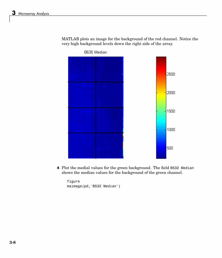
3 Microarray Analysis
MATLAB plots an image for the background of the red channel. Notice thevery high background levels down the right side of the array.
4 Plot the medial values for the green background. The field B532 Medianshows the median values for the background of the green channel.
figuremaimage(pd,'B532 Median')
3-8

Example: Visualizing Microarray Data
MATLAB plots an image for the background of the green channel.
5 The first array was for the Parkinson’s disease model mouse. Now read inthe data for the same brain voxel but for the untreated control mouse. Inthis case, the voxel sample was labeled with Cy3 and the control, totalbrain (not voxelated), was labeled with Cy5.
wt = gprread('mouse_a1wt.gpr')
MATLAB creates a structure and displays information about the structure.
3-9

3 Microarray Analysis
wt =Header: [1x1 struct]
Data: [9504x38 double]Blocks: [9504x1 double]
Columns: [9504x1 double]Rows: [9504x1 double]
Names: {9504x1 cell}IDs: {9504x1 cell}
ColumnNames: {38x1 cell}Indices: [132x72 double]
Shape: [1x1 struct]
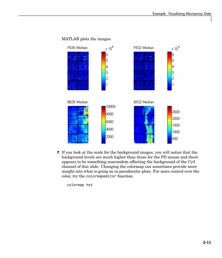
6 Use the function maimage to show pseudocolor images of the foregroundand background. You can use the function subplot to put all the plotsonto one figure.
figuresubplot(2,2,1);maimage(wt,'F635 Median')subplot(2,2,2);maimage(wt,'F532 Median')subplot(2,2,3);maimage(wt,'B635 Median')subplot(2,2,4);maimage(wt,'B532 Median')
3-10
Example: Visualizing Microarray Data
MATLAB plots the images.
7 If you look at the scale for the background images, you will notice that thebackground levels are much higher than those for the PD mouse and thereappears to be something nonrandom affecting the background of the Cy3channel of this slide. Changing the colormap can sometimes provide moreinsight into what is going on in pseudocolor plots. For more control over thecolor, try the colormapeditor function.
colormap hot
3-11

3 Microarray Analysis
MATLAB plots the images.
8 The function maimage is a simple way to quickly create pseudocolor imagesof microarray data. However if you want more control over plotting, it iseasy to create your own plots using the function imagesc.
First find the column number for the field of interest.
b532MedCol = find(strcmp(wt.ColumnNames,'B532 Median'))
MATLAB displays
b532MedCol =16
9 Extract that column from the field Data.
b532Data = wt.Data(:,b532MedCol);
3-12

Example: Visualizing Microarray Data
10 Use the field Indices to index into the Data.
figuresubplot(1,2,1);imagesc(b532Data(wt.Indices))axis imagecolorbartitle('B532 Median')
MATLAB plots the image.
3-13

3 Microarray Analysis
11 Bound the intensities of the background plot to give more contrast in theimage.
maskedData = b532Data;maskedData(b532Data<500) = 500;maskedData(b532Data>2000) = 2000;
subplot(1,2,2);imagesc(maskedData(wt.Indices))axis imagecolorbartitle('Enhanced B532 Median')
MATLAB plots the images.
3-14

Example: Visualizing Microarray Data
Statistics of the MicroarraysYou can use the function maboxplot to look at the distribution of data in eachof the blocks.
1 In the MATLAB Command Window, type
figuresubplot(2,1,1)maboxplot(pd,'F532 Median','title','Parkinson''s Disease Model Mouse')subplot(2,1,2)maboxplot(pd,'B532 Median','title','Parkinson''s Disease Model Mouse')figuresubplot(2,1,1)maboxplot(wt,'F532 Median','title','Untreated Mouse')subplot(2,1,2)maboxplot(wt,'B532 Median','title','Untreated Mouse')
MATLAB plots the images.
3-15

3 Microarray Analysis
2 Compare the plots.
From the box plots you can clearly see the spatial effects in the backgroundintensities. Blocks numbers 1, 3, 5, and 7 are on the left side of the arrays,and numbers 2, 4, 6, and 8 are on the right side. The data must benormalized to remove this spatial bias.
Scatter Plots of Microarray DataThere are two columns in the microarray data structure labeled 'F635 Median- B635' and 'F532 Median - B532'. These columns are the differencesbetween the median foreground and the median background for the 635 nmchannel and 532 nm channel respectively. These give a measure of the actualexpression levels, although since the data must first be normalized to removespatial bias in the background, you should be careful about using these valueswithout further normalization. However, in this example no normalizationis performed.
1 Rather than working with data in a larger structure, it is often easier toextract the column numbers and data into separate variables.
3-16

Example: Visualizing Microarray Data
cy5DataCol = find(strcmp(wt.ColumnNames,'F635 Median - B635'))cy3DataCol = find(strcmp(wt.ColumnNames,'F532 Median - B532'))cy5Data = pd.Data(:,cy5DataCol);cy3Data = pd.Data(:,cy3DataCol);
MATLAB displays
cy5DataCol =34
cy3DataCol =35
2 A simple way to compare the two channels is with a loglog plot. Thefunction maloglog is used to do this. Points that are above the diagonal inthis plot correspond to genes that have higher expression levels in the A1voxel than in the brain as a whole.
figuremaloglog(cy5Data,cy3Data)xlabel('F635 Median - B635 (Control)');ylabel('F532 Median - B532 (Voxel A1)');
MATLAB displays the following messages and plots the images.
Warning: Zero values are ignored(Type "warning off Bioinfo:MaloglogZeroValues" to suppressthis warning.)
Warning: Negative values are ignored.(Type "warning off Bioinfo:MaloglogNegativeValues" to suppressthis warning.)
3-17

3 Microarray Analysis
Notice that this function gives some warnings about negative and zeroelements. This is because some of the values in the 'F635 Median - B635'and 'F532 Median - B532' columns are zero or even less than zero. Spotswhere this happened might be bad spots or spots that failed to hybridize.Points with positive, but very small, differences between foreground andbackground should also be considered to be bad spots.
3 Disable the display of warnings by using the warning command. Althoughwarnings can be distracting, it is good practice to investigate why thewarnings occurred rather than simply to ignore them. There might be somesystematic reason why they are bad.
warnState = warning; % First save the current warningstate.
% Now turn off the two warnings.warning('off','Bioinfo:MaloglogZeroValues');warning('off','Bioinfo:MaloglogNegativeValues');figure
3-18

Example: Visualizing Microarray Data
maloglog(cy5Data,cy3Data) % Create the loglog plotwarning(warnState); % Reset the warning state.xlabel('F635 Median - B635 (Control)');ylabel('F532 Median - B532 (Voxel A1)');
MATLAB plots the image.
4 An alternative to simply ignoring or disabling the warnings is to removethe bad spots from the data set. You can do this by finding points whereeither the red or green channel has values less than or equal to a thresholdvalue. For example, use a threshold value of 10.
threshold = 10;badPoints = (cy5Data <= threshold) | (cy3Data <= threshold);
3-19

3 Microarray Analysis
MATLAB plots the image.
5 You can then remove these points and redraw the loglog plot.
cy5Data(badPoints) = []; cy3Data(badPoints) = [];figuremaloglog(cy5Data,cy3Data)xlabel('F635 Median - B635 (Control)');ylabel('F532 Median - B532 (Voxel A1)');
3-20

Example: Visualizing Microarray Data
MATLAB plots the image.
This plot shows the distribution of points but does not give any indicationabout which genes correspond to which points.
6 Add gene labels to the plot. Because some of the data points havebeen removed, the corresponding gene IDs must also be removed fromthe data set before you can use them. The simplest way to do that iswt.IDs(~badPoints).
maloglog(cy5Data,cy3Data,'labels',wt.IDs(~badPoints),'factorlines',2)
xlabel('F635 Median - B635 (Control)');ylabel('F532 Median - B532 (Voxel A1)');
3-21

3 Microarray Analysis
MATLAB plots the image.
7 Try using the mouse to click some of the outlier points.
You will see the gene ID associated with the point. Most of the outliers arebelow the y = x line. In fact, most of the points are below this line. Ideallythe points should be evenly distributed on either side of this line.
8 Normalize the points to evenly distribute them on either side of the line.Use the function mameannorm to perform global mean normalization.
normcy5 = mameannorm(cy5Data);normcy3 = mameannorm(cy3Data);
If you plot the normalized data you will see that the points are more evenlydistributed about the y = x line.
3-22

Example: Visualizing Microarray Data
figuremaloglog(normcy5,normcy3,'labels',wt.IDs(~badPoints),
'factorlines',2)xlabel('F635 Median - B635 (Control)');ylabel('F532 Median - B532 (Voxel A1)');
MATLAB plots the image.
9 The function mairplot is used to create an Intensity vs. Ratio plot for thenormalized data. This function works in the same way as the functionmaloglog.
figuremairplot(normcy5,normcy3,'labels',wt.IDs(~badPoints),
'factorlines',2)
3-23

3 Microarray Analysis
MATLAB plots the image.
10 You can click the points in this plot to see the name of the gene associatedwith the plot.
3-24

Example: Analyzing Gene Expression Profiles
Example: Analyzing Gene Expression ProfilesThis example demonstrates a number of ways to look for patterns in geneexpression profiles.
• “Exploring the Data Set” on page 3-25
• “Filtering Genes” on page 3-29
• “Clustering Genes” on page 3-32
• “Principal Component Analysis” on page 3-36
Overview of the Yeast ExampleThe microarray data for this example is from DeRisi, JL, Iyer, VR, and Brown,PO.; "Exploring the metabolic and genetic control of gene expression on agenomic scale"; Science, 1997, Oct 24;278(5338):680-6, PMID: 9381177.
The authors used DNA microarrays to study temporal gene expression ofalmost all genes in Saccharomyces cerevisiae during the metabolic shift fromfermentation to respiration. Expression levels were measured at seven timepoints during the diauxic shift. The full data set can be downloaded from theGene Expression Omnibus Web site at
http://www.ncbi.nlm.nih.gov/geo/query/acc.cgi?acc=GSE28
Exploring the Data Set
The data for this procedure is available in the MAT-file yeastdata.mat.This file contains the VALUE data or LOG_RAT2N_MEAN, or log2 of ratioof CH2DN_MEAN and CH1DN_MEAN from the seven time steps in theexperiment, the names of the genes, and an array of the times at which theexpression levels were measured.
1 Load data into MATLAB.
load yeastdata.mat
2 Get the size of the data by typing
numel(genes)
3-25

3 Microarray Analysis
MATLAB displays the number of genes in the data set. The MATLABvariable genes is a cell array of the gene names.
ans =6400
3 Access the entries using MATLAB cell array indexing.
genes{15}
MATLAB displays the 15th row of the variable yeastvalues, whichcontains expression levels for the open reading frame (ORF) YAL054C.
ans =YAL054C
4 Use the function web to access information about this ORF in theSaccharomyces Genome Database (SGD).
url = sprintf(...'http://genome-www4.stanford.edu/cgi-bin/SGD/locus.pl?locus=%s',...
genes{15});web(url);
5 A simple plot can be used to show the expression profile for this ORF.
plot(times, yeastvalues(15,:))xlabel('Time (Hours)');ylabel('Log2 Relative Expression Level');
3-26

Example: Analyzing Gene Expression Profiles
MATLAB plots the figure. The values are log2 ratios.
6 Plot the actual values.
plot(times, 2.^yeastvalues(15,:))xlabel('Time (Hours)');ylabel('Relative Expression Level');
3-27

3 Microarray Analysis
MATLAB plots the figure. The gene associated with this ORF, ACS1,appears to be strongly up-regulated during the diauxic shift.
7 Compare other genes by plotting multiple lines on the same figure.
hold onplot(times, 2.^yeastvalues(16:26,:)')xlabel('Time (Hours)');ylabel('Relative Expression Level');title('Profile Expression Levels');
3-28

Example: Analyzing Gene Expression Profiles
MATLAB plots the image.
Filtering GenesThe data set is quite large and a lot of the information corresponds to genesthat do not show any interesting changes during the experiment. To makeit easier to find the interesting genes, reduce the size of the data set byremoving genes with expression profiles that do not show anything of interest.There are 6400 expression profiles. You can use a number of techniques toreduce the number of expression profiles to some subset that contains themost significant genes.
1 If you look through the gene list you will see several spots marked as'EMPTY'. These are empty spots on the array, and while they might havedata associated with them, for the purposes of this example, you canconsider these points to be noise. These points can be found using thestrcmp function and removed from the data set with indexing commands..
3-29

3 Microarray Analysis
emptySpots = strcmp('EMPTY',genes);yeastvalues(emptySpots,:) = [];genes(emptySpots) = [];numel(genes)
MATLAB displays
ans =6314
In the yeastvalues data you will also see several places where theexpression level is marked as NaN. This indicates that no data was collectedfor this spot at the particular time step. One approach to dealing withthese missing values would be to impute them using the mean or median ofdata for the particular gene over time. This example uses a less rigorousapproach of simply throwing away the data for any genes where one ormore expression levels were not measured.
2 Use function isnan to identify the genes with missing data and then useindexing commands to remove the genes.
nanIndices = any(isnan(yeastvalues),2);yeastvalues(nanIndices,:) = [];genes(nanIndices) = [];numel(genes)
MATLAB displays
ans =6276
If you were to plot the expression profiles of all the remaining profiles, youwould see that most profiles are flat and not significantly different fromthe others. This flat data is obviously of use as it indicates that the genesassociated with these profiles are not significantly affected by the diauxicshift. However, in this example, you are interested in the genes with largechanges in expression accompanying the diauxic shift. You can use filteringfunctions in the Bioinformatics Toolbox to remove genes with various typesof profiles that do not provide useful information about genes affected bythe metabolic change.
3-30

Example: Analyzing Gene Expression Profiles
3 Use the function genevarfilter to filter out genes with small varianceover time. The function returns a logical array of the same size as thevariable genes with ones corresponding to rows of yeastvalues withvariance greater than the 10th percentile and zeros corresponding to thosebelow the threshold.
mask = genevarfilter(yeastvalues);% Use the mask as an index into the values to remove the% filtered genes.yeastvalues = yeastvalues(mask,:);genes = genes(mask);numel(genes)
MATLAB displays
ans =5648
4 The function genelowvalfilter removes genes that have very lowabsolute expression values. Note that the gene filter functions can alsoautomatically calculate the filtered data and names.
[mask, yeastvalues, genes] = genelowvalfilter(yeastvalues,genes,'absval',log2(4));
numel(genes)
MATLAB displays
ans =423
5 Use the function geneentropyfilter to remove genes whose profiles havelow entropy:
[mask, yeastvalues, genes] = geneentropyfilter(yeastvalues,genes,...'prctile',15);
numel(genes)
MATLAB displays
ans = 310
3-31
3 Microarray Analysis
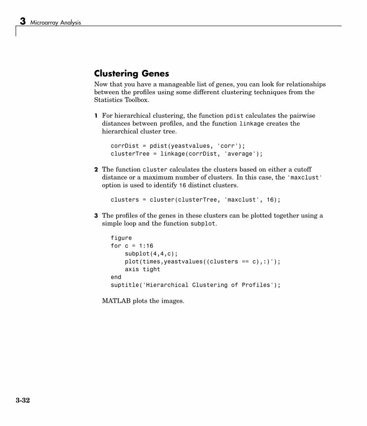
Clustering GenesNow that you have a manageable list of genes, you can look for relationshipsbetween the profiles using some different clustering techniques from theStatistics Toolbox.
1 For hierarchical clustering, the function pdist calculates the pairwisedistances between profiles, and the function linkage creates thehierarchical cluster tree.
corrDist = pdist(yeastvalues, 'corr');clusterTree = linkage(corrDist, 'average');
2 The function cluster calculates the clusters based on either a cutoffdistance or a maximum number of clusters. In this case, the 'maxclust'option is used to identify 16 distinct clusters.
clusters = cluster(clusterTree, 'maxclust', 16);
3 The profiles of the genes in these clusters can be plotted together using asimple loop and the function subplot.
figurefor c = 1:16
subplot(4,4,c);plot(times,yeastvalues((clusters == c),:)');axis tight
endsuptitle('Hierarchical Clustering of Profiles');
MATLAB plots the images.
3-32

Example: Analyzing Gene Expression Profiles
4 The Statistics Toolbox also has a K-means clustering function. Again,sixteen clusters are found, but because the algorithm is different these arenot necessarily the same clusters as those found by hierarchical clustering.
[cidx, ctrs] = kmeans(yeastvalues, 16,'dist','corr','rep',5,'disp','final');
figurefor c = 1:16
subplot(4,4,c);plot(times,yeastvalues((cidx == c),:)');axis tight
endsuptitle('K-Means Clustering of Profiles');
3-33

3 Microarray Analysis
MATLAB displays
13 iterations, total sum of distances = 11.404214 iterations, total sum of distances = 8.6267426 iterations, total sum of distances = 8.8606622 iterations, total sum of distances = 9.7767626 iterations, total sum of distances = 9.01035
5 Instead of plotting all of the profiles, you can plot just the centroids.
figurefor c = 1:16
subplot(4,4,c);plot(times,ctrs(c,:)');axis tightaxis off % turn off the axis
endsuptitle('K-Means Clustering of Profiles');
3-34

Example: Analyzing Gene Expression Profiles
MATLAB plots the figure.
6 You can use the function clustergram to create a heat map and dendrogramfrom the output of the hierarchical clustering.
figureclustergram(yeastvalues(:,2:end),'RowLabels',genes,...
'ColumnLabels',times(2:end))
3-35

3 Microarray Analysis
MATLAB plots the figure.
Principal Component AnalysisPrincipal-component analysis(PCA) is a useful technique you can use toreduce the dimensionality of large data sets, such as those from microarrayanalysis. PCA can also be used to find signals in noisy data.
1 You can use the The function princomp in the Statistics Toolbox to calculatethe principal components of a data set.
[pc, zscores, pcvars] = princomp(yeastvalues)
MATLAB displays
pc =
Columns 1 through 4
3-36

Example: Analyzing Gene Expression Profiles
-0.0245 -0.3033 -0.1710 -0.28310.0186 -0.5309 -0.3843 -0.54190.0713 -0.1970 0.2493 0.40420.2254 -0.2941 0.1667 0.17050.2950 -0.6422 0.1415 0.33580.6596 0.1788 0.5155 -0.50320.6490 0.2377 -0.6689 0.2601
Columns 5 through 7
-0.1155 0.4034 0.7887-0.2384 -0.2903 -0.3679-0.7452 -0.3657 0.2035-0.2385 0.7520 -0.42830.5592 -0.2110 0.1032-0.0194 -0.0961 0.0667-0.0673 -0.0039 0.0521
2 You can use the function cumsum to see the cumulative sum of the variances.
cumsum(pcvars./sum(pcvars) * 100)
MATLAB displays
ans =78.371989.214093.435796.083198.328399.3203
100.0000
This shows that almost 90% of the variance is accounted for by the firsttwo principal components.
3 A scatter plot of the scores of the first two principal components shows thatthere are two distinct regions. This is not unexpected, because the filteringprocess removed many of the genes with low variance or low information.These genes would have appeared in the middle of the scatter plot.
3-37

3 Microarray Analysis
figurescatter(zscores(:,1),zscores(:,2));xlabel('First Principal Component');ylabel('Second Principal Component');title('Principal Component Scatter Plot');
MATLAB plots the figure.
4 The function gname from the Statistics Toolbox can be used to identifygenes on a scatter plot. You can select as many points as you like on thescatter plot.
gname(genes);
When you have finished selecting points, press Enter.
3-38

Example: Analyzing Gene Expression Profiles
5 An alternative way to create a scatter plot is with the function gscatterfrom the Statistics Toolbox. gscatter creates a grouped scatter plot wherepoints from each group have a different color or marker. You can useclusterdata, or any other clustering function, to group the points.
figurepcclusters = clusterdata(zscores(:,1:2),6);gscatter(zscores(:,1),zscores(:,2),pcclusters)xlabel('First Principal Component');ylabel('Second Principal Component');title('Principal Component Scatter Plot with Colored Clusters');gname(genes) % Press enter when you finish selecting genes.
MATLAB plots the figure.
3-39

3 Microarray Analysis
3-40

4
Phylogenetic Analysis
Phylogenetic analysis is the process you use to determine the evolutionaryrelationships between organisms. The results of an analysis can be drawnin a hierarchical diagram called a cladogram or phylogram (phylogenetictree). The branches in a tree are based on the hypothesized evolutionaryrelationships (phylogeny) between organisms. Each member in a branch, alsoknown as a monophyletic group, is assumed to be descended from a commonancestor. Originally, phylogenetic trees were created using morphology, butnow, determining evolutionary relationships includes matching patterns innucleic acid and protein sequences.
“Example: Building a PhylogeneticTree” (p. 4-2)
Using data from mitochondrialD-loop sequences, create aphylogenetic tree for a familyof primates.
“Phylogenetic Tree Tool Reference”(p. 4-14)
Description of menu commands andfeatures for creating publishabletree figures.

4 Phylogenetic Analysis
Example: Building a Phylogenetic TreeIn this example, a phylogenetic tree is constructed from mitochondrial DNA(mtDNA) sequences for the family Hominidae. This family includes gorillas,chimpanzees, orangutans, and humans.
The following procedures demonstrate the phylogenetic analysis features inthe Bioinformatics Toolbox. They are not intended to teach the process ofphylogenetic analysis, but to show you how to use MathWorks products tocreate a phylogenetic tree from a set of nonaligned nucleotide sequences.
• “Overview for the Primate Example” on page 4-2 — Describes the biologicalbackground for this example.
• “Creating a Phylogenetic Tree for Five Species” on page 4-6 — Use theJukes-Cantor method to calculate distances between sequences, and theUnweighted Pair Group Method Average (UPGMA) method for linkingthe tree nodes.
• “Creating a Phylogenetic Tree for Twelve Species” on page 4-8 — Addadditional organisms to confirm the observed monophyletic groups.
• “Exploring the Phylogenetic Tree” on page 4-10 — Use the MATLABcommand-line interface to programmatically determine characteristics ina phylogenetic tree.
For information on how to create a phylogenetic tree with multiply alignedsequences, see the function —phytree.
Overview for the Primate ExampleThe origin of modern humans is a heavily debated issue that scientists haverecently tackled by using mitochondrial DNA (mtDNA) sequences. Onehypothesis explains the limited genetic variation of human mtDNA in termsof a recent common genetic ancestry, implying that all modern populationmtDNA originated from a single woman who lived in Africa less than 200,000years ago.
4-2
Example: Building a Phylogenetic Tree
Why use mitochondrial DNA sequences for phylogeneticstudy?Mitochondrial DNA sequences, like the Y chromosome, do not recombineand are inherited from the maternal parent. This lack of recombinationallows sequences to be traced through one genetic line and all polymorphismsassumed to be caused by mutations.
Mitochondrial DNA in mammals has a faster mutation rate than nuclearDNA sequences. This faster rate of mutation produces more variance betweensequences and is an advantage when studying closely related species. Themitochondrial control region (Displacement or D-loop) is one of the fastestmutating sequence regions in animal DNA.
Neanderthal DNAThe ability to isolate mitochondrial DNA (mtDNA) from palaeontologicalsamples has allowed genetic comparisons between extinct species and closelyrelated nonextinct species. The reasons for isolating mtDNA instead ofnuclear DNA in fossil samples have to do with the fact that
• mtDNA, because it is circular, is more stable and degrades slower thennuclear DNA.
• Each cell can contain a thousand copies of mtDNA and only a single copyof nuclear DNA.
While there is still controversy as to whether Neanderthals are directancestors of humans or evolved independently, the use of ancient geneticsequences in phylogenetic analysis adds an interesting dimension to thequestion of human ancestry.
ReferencesOvchinnikov, I., et al., 2000. "Molecular analysis of Neanderthal DNA fromthe northern Caucasus," Nature 404(6777), pp 490-493.
Sajantila, A., et al., 1995. "Genes and languages in Europe: an analysis ofmitochondrial lineages," Genome Res. 5 (1), pp. 42-52 (1995).
Krings, M., et al., 1997. "Neanderthal DNA sequences and the origin ofmodern humans," Cell 90 (1), pp. 19-30.
4-3

4 Phylogenetic Analysis
Jensen-Seaman, M., and K. Kidd, 2001. "Mitochondrial DNA variation andbiogeography of eastern gorillas," Mol. Ecol. 10(9), pp. 2241-2247.
Searching NCBI for Phylogenetic DataThe NCBI taxonomy Web site includes phylogenetic and taxonomicinformation from many sources. These sources include the publishedliterature, Web databases, and taxonomy experts. And while the NCBItaxonomy database is not a phylogenetic or taxonomic authority, it can beuseful as a gateway to the NCBI biological sequence databases.
This procedure uses the family Hominidae (orangutans, chimpanzees,gorillas, and humans) as a taxonomy example for searching the NCBI Website and locating mitochondrial D-loop sequences.
1 Use the MATLAB Help browser to search for data on the Web. In theMATLAB Command Window, type
web('http://www.ncbi.nlm.nih.gov')
A separate browser window opens with the home page for the NCBI Website.
2 Search the NCBI Web site for information. For example, to search for thehuman taxonomy, from the Search list, select Taxonomy, and in the forbox, enter hominidae.
The NCBI Web search returns a list of links to relevant pages.
4-4

Example: Building a Phylogenetic Tree
3 Select the taxonomy link for the family Hominidae. A page with thetaxonomy for the family is shown.
4-5

4 Phylogenetic Analysis
Creating a Phylogenetic Tree for Five SpeciesDrawing a phylogenetic tree using sequence data is helpful when you aretrying to visualize the evolutionary relationships between species. Thesequences can be multiply aligned or a set of nonaligned sequences, you canselect a method for calculating pairwise distances between sequences, andyou can select a method for calculating the hierarchical clustering distancesused to build a tree.
4-6

Example: Building a Phylogenetic Tree
After locating the GenBank accession codes for the sequences you areinterested in studying, you can create a phylogenetic tree with the data. Forinformation on locating accession codes, see “Searching NCBI for PhylogeneticData” on page 4-4.
1 Create a MATLAB structure with information about the sequences. Thisstep uses the accession codes for the mitochondrial D-loop sequencesisolated from different hominid species.
data = {'German_Neanderthal' 'AF011222';'Russian_Neanderthal' 'AF254446';'European_Human' 'X90314' ;'Mountain_Gorilla_Rwanda' 'AF089820';'Chimp_Troglodytes' 'AF176766';};
2 Get sequence data from the GenBank database and copy into MATLAB.
for ind = 1:5seqs(ind).Header = data{ind,1};seqs(ind).Sequence = getgenbank(data{ind,2},
'sequenceonly', true);end
3 Calculate pairwise distances and create a phytree object. For example,compute the pairwise distances using the Jukes-Cantor distance methodand build a phylogenetic tree using the UPGMA linkage method. Sincethe sequences are not prealigned, seqpdist pairwise aligns them beforecomputing the distances.
distances = seqpdist(seqs,'Method','Jukes-Cantor','Alphabet','DNA');tree = seqlinkage(distances,'UPGMA',seqs)
MATLAB displays information about the phytree object. The functionseqpdist calculates the pairwise distances between pairs of sequenceswhile the function seqlinkage uses the distances to build a hierarchicalcluster tree. First, the most similar sequences are grouped together, andthen sequences are added to the tree in decending order of similarity.
Phylogenetic tree object with 5 leaves (4 branches)
4-7

4 Phylogenetic Analysis
4 Draw a phylogenetic tree.
h = plot(tree,'orient','bottom');ylabel('Evolutionary distance')set(h.terminalNodeLabels,'Rotation',-45)
MATLAB draws a phylogenetic tree in a figure window. In the figurebelow, the hypothesized evolutionary relationships between the species. isshown by the location of species on the branches shows the The horizontaldistances do not have any biological significance.
Creating a Phylogenetic Tree for Twelve SpeciesPlotting a simple phylogenetic tree for five species seems to indicate a numberof monophyletic groups(see “Creating a Phylogenetic Tree for Five Species” on
4-8

Example: Building a Phylogenetic Tree
page 4-6). After a preliminary analysis with five species, you can add morespecies to your phylogenetic tree. Adding more species to the data set willhelp you to confirm the groups are valid.
1 Add more sequences to a MATLAB structure. For example, add mtDNAD-loop sequences for other hominid species.
data2 = {'Puti_Orangutan' 'AF451972';'Jari_Orangutan' 'AF451964';'Western_Lowland_Gorilla' 'AY079510';'Eastern_Lowland_Gorilla' 'AF050738';'Chimp_Schweinfurthii' 'AF176722';'Chimp_Vellerosus' 'AF315498';'Chimp_Verus' 'AF176731';
};
2 Get additional sequence data from the GenBank database, and copy thedata into the next indices of a MATALB structure.
for ind = 1:7seqs(ind+5).Header = data2{ind,1};seqs(ind+5).Sequence = getgenbank(data2{ind,2},
'sequenceonly', true);end
3 Calculate pairwise distances and the hierarchical linkage.
distances = seqpdist(seqs,'Method','Jukes-Cantor','Alpha','DNA');tree = seqlinkage(distances,'UPGMA',seqs);
4 Draw a phylogenetic tree.
h = plot(tree,'orient','bottom');ylabel('Evolutionary distance')set(h.terminalNodeLabels,'Rotation',-45)
MATLAB draws a phylogenetic tree in a figure window. You can see fourmain clades for humans, gorillas, chimpanzee, and orangutans.
4-9

4 Phylogenetic Analysis
Exploring the Phylogenetic TreeAfter you create a phylogenetic tree, you can explore the tree using theMATLAB command line or the phytreetool GUI. This procedure uses thetree created in “Creating a Phylogenetic Tree for Twelve Species” on page4-8 as an example.
1 List the members of a tree.
names = get(tree,'LeafNames')
From the list, you can determine the indices for its members. For example,the European Human leaf is the third entry.
names =
4-10

Example: Building a Phylogenetic Tree
'German_Neanderthal''Russian_Neanderthal''European_Human''Chimp_Troglodytes''Chimp_Schweinfurthii''Chimp_Verus''Chimp_Vellerosus''Puti_Orangutan''Jari_Orangutan''Mountain_Gorilla_Rwanda''Eastern_Lowland_Gorilla''Western_Lowland_Gorilla'
2 Find the closest species to a selected specie in a tree. For example, find thespecies closest to the European human.
[h_all,h_leaves] = select(tree,'reference',3,'criteria','distance','threshold',0.6);
h_all is a list of indices for the nodes within a patristic distance of 0.6 tothe European human leaf, while h_leaves is a list of indices for only theleaf nodes within the same patristic distance.
A patristic distance is the path length between species calculated fromthe hierarchical clustering distances. The path distance is not necessarilythe biological distance.
3 List the names of the closest species.
subtree_names = names(h_leaves)
MATLAB prints a list of species with a patristic distance to the Europeanhuman less than the specified distance. In this case, the patristic distancethreshold is less than 0.6.
subtree_names =
'German_Neanderthal''Russian_Neanderthal''European_Human''Chimp_Schweinfurthii'
4-11
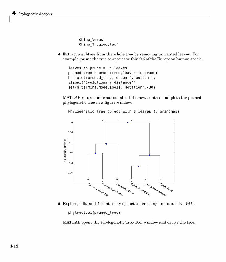
4 Phylogenetic Analysis
'Chimp_Verus''Chimp_Troglodytes'
4 Extract a subtree from the whole tree by removing unwanted leaves. Forexample, prune the tree to species within 0.6 of the European human specie.
leaves_to_prune = ~h_leaves;pruned_tree = prune(tree,leaves_to_prune)h = plot(pruned_tree,'orient','bottom');ylabel('Evolutionary distance')set(h.terminalNodeLabels,'Rotation',-30)
MATLAB returns information about the new subtree and plots the prunedphylogenetic tree in a figure window.
Phylogenetic tree object with 6 leaves (5 branches)
5 Explore, edit, and format a phylogenetic tree using an interactive GUI.
phytreetool(pruned_tree)
MATLAB opens the Phylogenetic Tree Tool window and draws the tree.
4-12

Example: Building a Phylogenetic Tree
You can interactively change the appearance of the tree within the toolwindow. For information on using this GUI, see “Phylogenetic Tree ToolReference” on page 4-14.
4-13

4 Phylogenetic Analysis
Phylogenetic Tree Tool ReferenceThe Phylogenetic Tree Tool is an interactive graphical user interface (GUI)that allows you to view, edit, format, and explore phylogenetic tree data. Withthis GUI you can prune, reorder, rename branches, and explore distances.You can also open or save Newick formatted files.
• “Opening the Phytreetool GUI” on page 4-14 — Draw a phylogenetic treefrom data in a phytree object or a previously saved file.
• “File Menu” on page 4-16 — Open tree data from a Newick formattedfile, copy data to a MATLAB figure window, another tool window, or theMATLAB workspace, and save tree data.
• “Tools Menu” on page 4-24 — Explore branch paths, rename and edit branchand leaf names, hide selected branches and leaves, and rotate branches.
• “Windows Menu” on page 4-32 — Switch to any open window.
• “Help Menu” on page 4-32 — Select quick links to the BioinformaticsToolbox documentation for phylogenetic analysis functions, tutorials, andthe phytreetool reference.
Opening the Phytreetool GUIThe Phylogenetic Tree Tool can read data from Newick and ClustalW treeformatted files.
This procedure uses the phylogenetic tree data stored in the file pf00002.treeas an example. The data was retrieved from the protein family (PFAM) Webdatabase and saved to a file using the accession number PF00002 and thefunction gethmmtree.
1 Create a phytree object. For example, to create a phytree object from treedata in the file pf00002.tree, type
tr= phytreeread('pf00002.tree')
MATLAB creates a phytree object.
Phylogenetic tree object with 37 leaves (36 branches)
2 Open the Phylogenetic Tree Tool and draw a phylogenetic tree.
4-14
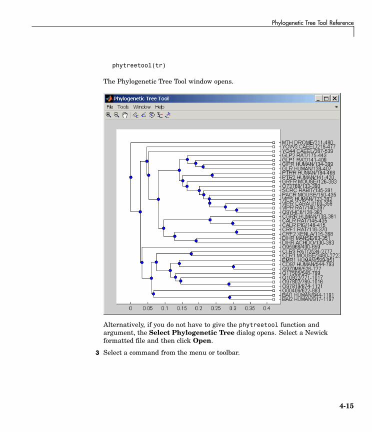
Phylogenetic Tree Tool Reference
phytreetool(tr)
The Phylogenetic Tree Tool window opens.
Alternatively, if you do not have to give the phytreetool function andargument, the Select Phylogenetic Tree dialog opens. Select a Newickformatted file and then click Open.
3 Select a command from the menu or toolbar.
4-15

4 Phylogenetic Analysis
File MenuThe File menu includes the standardcommands for opening and closing afile, and it includes commands to usephytree object data from the MATLABworkspace.The File menu commandsare shown below.
New Tool CommandUse the New Tool command to open tree data from a file into a secondPhylogenetic Tree Tool window.
1 From the File menu, click New Tool.
The Select Phylogenetic Tree File dialog opens.
2 Select a directory and select a file with the extension .tree, and thenclick Open. The Bioinformatics Toolbox uses the file extension .tree forNewick formatted files, but you can use any Newick formatted file withany extension.
4-16

Phylogenetic Tree Tool Reference
MATLAB opens a second Phylogenetic Tree Tool window with tree datafrom the selected file.
Open CommandUse the Open command to read tree data from a Newick formatted file anddisplay that data in a Phylogenetic Tree Tool.
1 From the File menu, click Open.
The Select Phylogenetic Tree File dialog box opens.
2 Select a directory, select a Newick formatted file, and then click Open. TheBioinformatics Toolbox uses the file extension .tree for Newick formattedfiles, but you can use any Newick formatted file with any extension.
MATLAB replaces the current tree data with data from the selected file.
Open from Workspace CommandUse the Open from Workspace command to read tree data from a phytreeobject in the MATLAB workspace and display that data in a PhylogeneticTree Tool.
1 From the File menu, click Open from Workspace.
The Get Phytree Object dialog box opens.
4-17
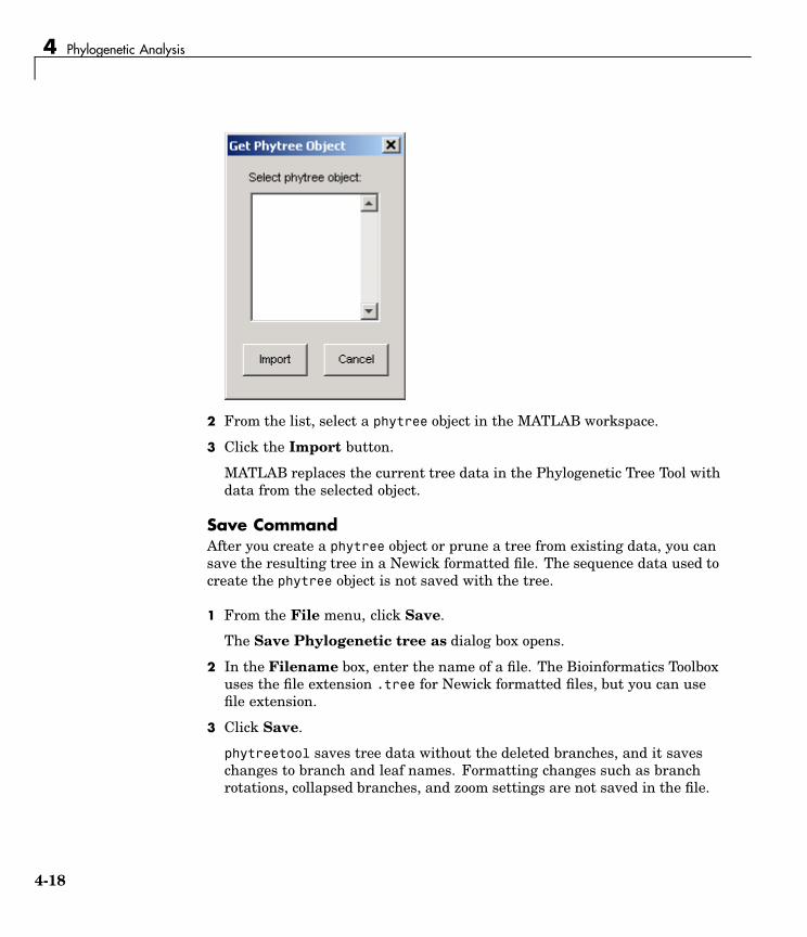
4 Phylogenetic Analysis
2 From the list, select a phytree object in the MATLAB workspace.
3 Click the Import button.
MATLAB replaces the current tree data in the Phylogenetic Tree Tool withdata from the selected object.
Save CommandAfter you create a phytree object or prune a tree from existing data, you cansave the resulting tree in a Newick formatted file. The sequence data used tocreate the phytree object is not saved with the tree.
1 From the File menu, click Save.
The Save Phylogenetic tree as dialog box opens.
2 In the Filename box, enter the name of a file. The Bioinformatics Toolboxuses the file extension .tree for Newick formatted files, but you can usefile extension.
3 Click Save.
phytreetool saves tree data without the deleted branches, and it saveschanges to branch and leaf names. Formatting changes such as branchrotations, collapsed branches, and zoom settings are not saved in the file.
4-18

Phylogenetic Tree Tool Reference
Publish to Figure CommandAfter you have explored the relationships between branches and leaves inyour tree, you can copy the tree to a MATLAB figure window. Using a figurewindow allows you to use all the MATLAB features for annotating, changingfont characteristics, and getting your figure ready for publication. Also, fromthe figure window, you can save an image of the tree as it was displayed inthe Phylogenetic Tree Tool window.
1 From the File menu, point to Publish to Figure, and then click eitherWith Hidden Nodes or Only Displayed.
The Publish Phylogenetic Tree to Figure dialog box opens.
2 Select one of the Rendering Types, and then select the Display Labels youwant on your figure.
• Dendrogram (square branches)
4-19
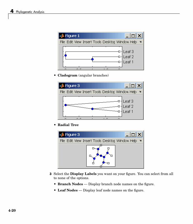
4 Phylogenetic Analysis
• Cladogram (angular branches)
• Radial Tree
3 Select the Display Labels you want on your figure. You can select from allto none of the options.
• Branch Nodes — Display branch node names on the figure.
• Leaf Nodes — Display leaf node names on the figure.
4-20

Phylogenetic Tree Tool Reference
• Terminal Nodes — Display terminal node names on the right border.
4 Click the Publish button.
A new figure window opens with the characteristics you selected.
Export to New Tool CommandBecause some of the Phylogenetic Tree Tool commands cannot be undone (forexample, the Prune command), you might want to make a copy of your treebefore trying a command. At other times, you might want to compare twoviews of the same tree, and copying a tree to a new tool window allows you tomake changes to both tree views independently .
1 From the File menu, point to the Export to New Tool submenu, and thenclick either With Hidden Nodes or Only Displayed.
A new Phylogenetic Tree Tool window opens with a copy of the tree.
2 Use the new figure to continue your analysis.
Export to Workspace CommandThe Phylogenetic Tree Tool can open Newick formatted files with tree data.However, it does not create a phytree object in the MATLAB workspace. Ifyou want to programmatically explore phylogenetic trees, you need to usethe Export to Workspace command.
1 From the File menu, point to Export to Workspace, and then click eitherWith Hidden Nodes or Only Displayed.
The Export to Workspace dialog box opens.
2 In the MATLAB variable name box, enter the name for your phylogenetictree data.
4-21

4 Phylogenetic Analysis
3 Click OK.
MATLAB creates an object in the MATLAB workspace with type phytree.
Page Setup CommandWhen you print from the Phylogenetic Tree Tool or a MATLAB figure window(with a tree published from the tool), you can specify setup options forprinting a tree.
1 From the File menu, click Page Setup.
The Page Setup - Phylogenetic Tree Tool dialog box opens. This is thesame dialog box MATLAB uses to select page formatting options.
2 Select the page formatting options and values you want, and then click OK.
Print Setup CommandUse the Print Setup command with the Page Setup command to print aMATLAB figure window.
4-22

Phylogenetic Tree Tool Reference
1 From the File menu, click Print Setup.
The Print Setup dialog box opens.
2 Select the printer and options you want, and then click OK.
Print Preview CommandUse the Print Preview command to check the formatting options youselected with the Page Setup commend.
1 From the File menu, click Print Preview.
A window opens with a picture of your figure with the selected formattingoptions.
2 Click Print or Close.
PrintUse the Print command to make a copy of your phylogenetic tree after youuse the Page Setup command to select formatting options.
4-23

4 Phylogenetic Analysis
1 From the File menu, click Print.
The Print dialog box opens.
2 From the Name list, select a printer, and then click OK.
Tools MenuThe Tools menu and toolbar are whereyou will find most of the commandsspecific to trees and phylogeneticanalysis. Use these commands and modesto interactively edit and format your tree.The Tools menu commands are shownbelow.
Inspect Mode CommandUse the inspect mode to compare path distances between sequences and tosearch for related sequences that might not be physically drawn close together.
1 From the Tools menu, click Inspect, or from the toolbar, click the Inspect
Tool mode icon .
The Phylogenetic Tree Tool is set to inspect mode.
2 Point to a branch or leaf node.
4-24

Phylogenetic Tree Tool Reference
A pop-up window opens with information about the patristic distances toparent and root nodes.
3 Click a branch or leaf node, and then move your mouse over another leafnode.
The tool highlights the path between nodes and displays the path length inthe pop-up window . The path length is the patristic distances calculatedby seqlinkage.
Collapse/Expand Branch Mode CommandSome trees can have thousands of leaf and branch nodes. Displaying all thenodes can create a tree diagram that is unreadable. By collapsing some of thebranches, you can better see the relationships between the remaining nodes.
1 From the Tools menu, click Collapse/Expand, or from the toolbar, click
the Collapse/Expand node icon .
The Phylogenetic Tree Tool is set to collapse/expand mode.
2 Point to a branch.
The selected paths to collapse (remove from view) are highlighted in gray.
4-25

4 Phylogenetic Analysis
3 Click the branch node.
The tool removes the display of branch and leaf nodes below the selectedbranch. The data is not removed.
4 To expand a branch, point to a collapsed branch and click.
Rotate Branch Mode CommandA phylogenetic tree is initially created by pairing the two most similarsequences and then adding the remaining sequences in a decreasing orderof similarity. You might want to rotate branches to emphasize the directionof evolution.
1 From the Tools menu, click Rotate Branch, or from the toolbar, click
the Rotate Branch mode icon .
The Phylogenetic Tree Tool is set to rotate branch mode.
2 Point to a branch node.
3 Click the branch node.
4-26
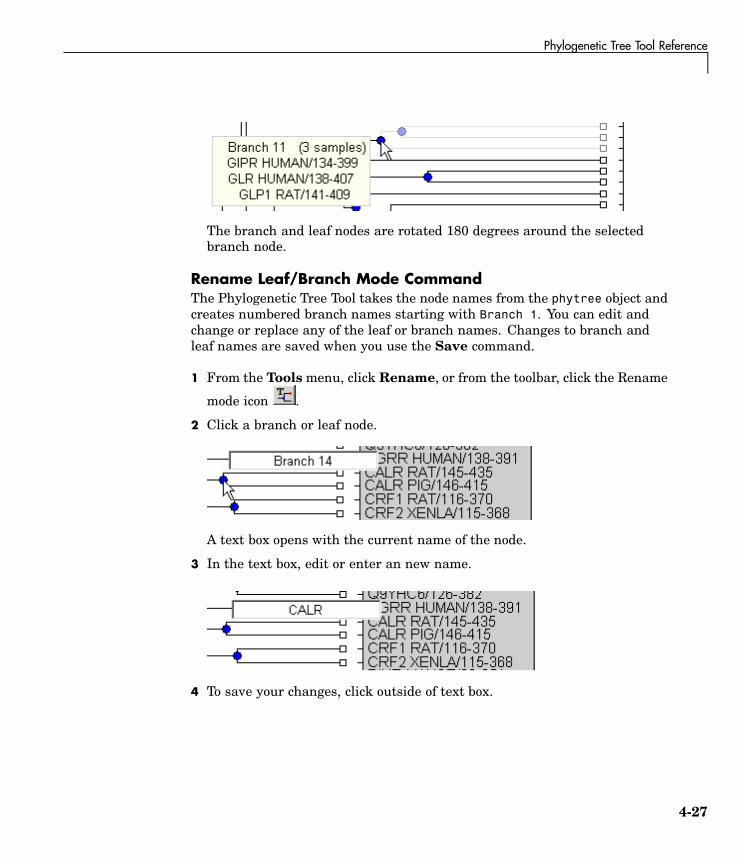
Phylogenetic Tree Tool Reference
The branch and leaf nodes are rotated 180 degrees around the selectedbranch node.
Rename Leaf/Branch Mode CommandThe Phylogenetic Tree Tool takes the node names from the phytree object andcreates numbered branch names starting with Branch 1. You can edit andchange or replace any of the leaf or branch names. Changes to branch andleaf names are saved when you use the Save command.
1 From the Tools menu, click Rename, or from the toolbar, click the Rename
mode icon .
2 Click a branch or leaf node.
A text box opens with the current name of the node.
3 In the text box, edit or enter an new name.
4 To save your changes, click outside of text box.
4-27

4 Phylogenetic Analysis
Prune (delete) Leaf/Branch Mode CommandYour tree might contain leaves that are far outside the phylogeny, or it mighthave duplicate leaves that you want to remove.
1 From the Tools menu, click Prune, or from the toolbar, click the prune
icon .
The Phylogenetic Tree Tool is set to rename mode.
2 Point to a branch or leaf node.
For leaf node, the branch line connected to the leaf is highlighted in gray.For a branch nodes, the branch lines below the node are highlighted inlight gray.
Note If you delete nodes (branches or leaves), you cannot undo thechanges. The Phylogenetic Tree Tool does not have an Undo command.
3 Click the branch or leaf node.
The branch is removed from the figure and the other nodes are rearrangedto balance the tree structure. The phylogeny is not recalculated.
Zoom In, Zoom Out, and Pan CommandsThe Zoom and Pan commands are the standard controls with MATLAB figuresfor resizing and moving the screen.
1 From the Tools menu, click Zoom In, or from the toolbar click the zoom
in icon .
4-28

Phylogenetic Tree Tool Reference
The tool activates zoom n mode and changes the cursor to a magnifyingglass.
2 Place the cursor over the section of the tree diagram you want to enlargeand then click.
The tree diagram is enlarged to twice its size.
3 From the toolbar click the Pan icon .
4 Move the cursor over the tree diagram, left-click, and drag the diagram tothe location you want to view.
Zoom In , Zoom Out , Pan
Threshold Collapse CommandUse the Threshold Collapse command to collapse the display of nodesusing a distance criterion instead of interactively selecting nodes with theCollapse/Expand command. Branches with distances below the thresholdare collapsed from the display.
1 From the Tools menu, click Threshold Collapse, and select one of thefollowing:
4-29

4 Phylogenetic Analysis
• Distance to Leaves — Sets the threshold starting from the right ofthe tree.
• Distance to Root — Sets the threshold starting from the root nodeat the left side of the tree.
The collapse slider bar is displayed at the top of the diagram.
2 Click and drag the slider bar to the left to set the distance threshold.
3 Click the OK button to the right of the slider. The nodes below the distancethreshold are hidden.
4-30

Phylogenetic Tree Tool Reference
Expand All CommandThe data for branches and leaves you hide with the Collapse/Expand orThreshold Collapse commands is not removed from the tree. You candisplay the hidden data using these commands or display all hidden data withthe Expand All command.
1 From the Tool menu, click Expand All. The hidden branches and leavesare displayed.
Find Leaf/Branch CommandPhylogenetic trees can have thousands of leaves and branches, and finding aspecific node can be difficult. Use the Find command to locate a node usingits name or part of its name.
1 From the Tools menu, click Find Leaf/Branch.
The Find Leaf/Branch dialog opens.
2 In the Regular Expression to match box, enter a name or partial nameof a branch or leaf.
3 Click OK.
4-31

4 Phylogenetic Analysis
Fit to WindowAfter you hide nodes with the Collapse/Expand or Threshold Collapsecommands, or delete nodes with the Prune command, there might be extraspace in the tree diagram. Use the Fit to Window command to redraw thetree diagram to fill the entire figure window.
1 From the Tools menu, click Fit to Window.
Reset View CommandUse the Reset Window command to remove formatting changes such asrotations, collapsed branches, and zooms.
1 From the Tools menu, click Reset Window.
Options SubmenuUse the Options command to select the behavior for the zoom and pan modes.
• Unconstrained Zoom — Allow zooming in both horizontal and verticaldirections.
• Horizontal Zoom — Restrict zoom to the horizontal direction.
• Vertical Zoom — Zoom only in the vertical direction (default).
• Unconstrained Pan — Allow panning in both horizontal and verticaldirections.
• Horizontal Pan — Restrict panning to horizontal direction.
• Vertical Pan — Pan only in the vertical direction (default).
Windows MenuThe Windows menu is standard on MATLAB GUI and figure windows. Usethis menu to select any opened window.
Help MenuUse the Help menu to select quick links to the Bioinformatics Toolboxdocumentation for phylogenetic analysis functions, tutorials, and thephytreetool reference.
4-32

5
Functions – Categorical List
This chapter is a reference for the functions in the Bioinformatics Toolbox.Functions are grouped into the following categories.
“Data Formats and Databases” on page5-2
“Sequence Conversion” on page 5-4
“Sequence Statistics” on page 5-5
“Sequence Utilities” on page 5-6
“Pairwise Sequence Alignment” on page5-7
“Profile Hidden Markov Models” on page5-10
“Scoring Matrices” on page 5-14
“Trace Tools” on page 5-9
“Microarray File Formats” on page 5-11
“Microarray Visualization” on page 5-12
“Microarray Normalization and Filtering”on page 5-13
“Protein Analysis” on page 5-8
“Phylogenetic Tree Tools” on page 5-15
“Phylogenetic Tree Methods” on page 5-16
“Tutorials, Demos, and Examples” onpage 5-17

5 Functions – Categorical List
Data Formats and DatabasesUse these functions to get data from Web data bases into MATLAB, and readand write to files within MATLAB using specific data formats.
blastread Read an BLAST report from a file
emblread Read data from an EMBL file
fastaread Read data from a FASTA formattedfile
fastawrite Write to a file using a FASTA format
galread Read microarray data from aGenePix array list file
genbankread Read data from a GenBank file
genpeptread Read data from a GenPept file
geosoftread Read data from a Gene ExpressionOmnibus (GEO) SOFT file
getblast Get BLAST report from NCBI website
getembl Retrieve sequence information fromthe EMBL database
getgenbank Retrieve sequence information fromthe GenBank database
getgenpept Retrieve sequence information fromthe GenPept database
getgeodata Get Gene Expression Omnibus(GEO) data
gethmmalignment Retrieve multiple aligned sequencesfrom the PFAM database
gethmmprof Retrieve profile hidden Markovmodels from the PFAM database
gethmmtree Get phylogenetic tree data fromPFAM database
5-2

Data Formats and Databases
getpdb Retrieve protein structureinformation from the PDB database
getpir Retrieve sequence data from thePIR-PSD database
gprread Read microarray data from aGenePix Results (GPR) file
imageneread Read microarray data from anImaGene Results file
multialignread Read a multiple sequence alignmentfile
pdbread Read data from a Protein Data Bank(PDB) file
pfamhmmread Read data from a PFAM-HMM file
phytreeread Read phylogenetic tree files
pirread Read data from a PIR file
scfread Read trace data from a SCF file
sptread Read data from a SPOT file
5-3

5 Functions – Categorical List
Sequence ConversionConvert nucleotide and amino acid sequences.
aa2int Convert an amino acid sequence froma letter to an integer representation
aa2nt Convert an amino acid sequence to anucleotide sequence
aminolookup Display amino acid codes, integers,abbreviations, names, and codons
baselookup Display nucleotide codes, integers,names, and abbreviations
dna2rna Convert a DNA sequence to an RNAsequence
int2aa Convert an amino acid sequence froman integer to a letter representation
int2nt Convert a nucleotide sequence froman integer to a letter representation
nt2aa Convert a sequence of nucleotides toa sequence of amino acids
nt2int Convert a nucleotide sequence froma letter to an integer representation
rna2dna Convert an RNA sequence ofnucleotides to a DNA sequence
seq2regexp Convert a sequence with ambiguouscharacters to a regular expression
seqcomplement Calculate the complementary strandof a nucleotide sequence
seqrcomplement Calculate the reverse complement ofa nucleotide sequence
seqreverse Reverse the letters or numbers in anucleotide sequence
5-4

Sequence Statistics
Sequence StatisticsList of sequence statistics functions
aacount Count the amino acids in a sequence
aminolookup Display amino acid codes, integers,abbreviations, names, and codons
basecount Count the number of nucleotides ina sequence
baselookup Display nucleotide codes, integers,names, and abbreviations
codoncount Count the number of codons in anucleotide sequence
dimercount Count the number of dimers in asequence
nmercount Count the number of n-mers in anucleotide or amino acid sequence
ntdensity Plot the density of nucleotides alonga sequence
seqshowwords Graphically display the words in asequence
seqwordcount Count the number of occurrences ofa word in a sequence
5-5

5 Functions – Categorical List
Sequence UtilitiesList of sequence utilities functions
aminolookup Display amino acid codes, integers,abbreviations, names, and codons
baselookup Display nucleotide codes, integers,names, and abbreviations
blastncbi Generate a remote BLAST request
geneticcode Return nucleotide codon to aminoacid mapping
joinseq Join two sequences to produce theshortest supersequence
palindromes Find palindromes in a sequence
randseq Generate a random sequence froma finite alphabet
restrict Split a sequence at a specifiedrestriction site
revgeneticcode Get the reverse mapping for agenetic code
seqdisp Format long sequence output foreasy viewing
seqmatch Find matches for every string in alibrary
seqshoworfs Graphically display the open readingframes in a sequence
5-6

Pairwise Sequence Alignment
Pairwise Sequence AlignmentList of pairwise sequence alignment functions
nwalign Globally align two sequences usingthe Needleman-Wunsch algorithm
seqdotplot Create a dot plot of two sequences
showalignment Display a sequence alignment withcolor
swalign Locally align two sequences usingthe Smith-Waterman algorithm
5-7

5 Functions – Categorical List
Protein AnalysisList of protein analysis functions
aacount Count the amino acids in a sequence
aminolookup Display amino acid codes, integers,abbreviations, names, and codons
atomiccomp Calculate the atomic composition ofa protein
cleave Cleave a protein with an enzyme
isoelectric Estimate the isoelectric point for anamino acid sequence
molweight Calculate the molecular weight of anamino acid sequence
pdbdistplot Visualize the intermoleculardistances in a PDB file
proteinplot Display property values for aminoacid sequences
ramachandran Draw a Ramachandran plot for PDBdata
5-8
Trace Tools
Trace ToolsList of functions for analysis of nucleotide traces
scfread Read trace data from a SCF file
traceplot Draw nucleotide trace plots
5-9

5 Functions – Categorical List
Profile Hidden Markov ModelsList of Hidden Markov Model functions
gethmmalignment Retrieve multiple aligned sequencesfrom the PFAM database
gethmmprof Retrieve profile hidden Markovmodels from the PFAM database
hmmprofalign Align a query sequence to a profileusing hidden Markov model basedalignment
hmmprofestimate Estimate profile HMM parametersusing pseudocounts
hmmprofgenerate Generate a random sequence drawnfrom the profile HMM
hmmprofmerge Concatenate the prealigned stringsof several sequences to a profileHMM
hmmprofstruct Create a profile HMM structure
pfamhmmread Read data from a PFAM-HMM file
showhmmprof Plot an HMM profile
5-10

Microarray File Formats
Microarray File FormatsList of microarray file format functions
affyread Read microarray data from anAffymetrix GeneChip file
galread Read microarray data from aGenePix array list file
geosoftread Read data from a Gene ExpressionOmnibus (GEO) SOFT file
getgeodata Get Gene Expression Omnibus(GEO) data
gprread Read microarray data from aGenePix Results (GPR) file
imageneread Read microarray data from anImaGene Results file
sptread Read data from a SPOT file
5-11

5 Functions – Categorical List
Microarray VisualizationList of microarray visualization functions
clustergram Create a dendrogram and heat mapon the same figure
maboxplot Display a box plot for microarraydata
maimage Display a spatial image formicroarray data
mairplot Display intensity versus ratio scatterplot for microarray signals
maloglog Create a loglog plot of microarraydata
mapcaplot Creates a Principal Component plotof expression profile data
redgreencmap Display a red and green colormap
5-12

Microarray Normalization and Filtering
Microarray Normalization and FilteringList of microarray normalization and filtering functions
exprprofrange Calculate the range of geneexpression profiles
exprprofvar Calculate the variance of geneexpression profiles
geneentropyfilter Remove genes with low entropyexpression values
genelowvalfilter Remove gene profiles with lowabsolute values
generangefilter Remove gene profiles with smallprofile ranges
genevarfilter Filter genes with small profilevariance
malowess Smooth microarray data using theLowess method
mamadnorm Normalize microarray data bymedian absolute deviation (MAD)
mameannorm Normalize microarray data usingthe global mean
5-13

5 Functions – Categorical List
Scoring MatricesList of scoring matrices
blosum Return a BLOSUM scoring matrix
dayhoff Return a Dayhoff scoring matrix
gonnet Return a Gonnet scoring matrix
nuc44 Return a NUC44 scoring matrix fornucleotide sequences
pam Return a PAM scoring matrix
5-14

Phylogenetic Tree Tools
Phylogenetic Tree ToolsList of functions for phylogenetic tree analysis.
gethmmtree Get phylogenetic tree data fromPFAM database
phytreeread Read phylogenetic tree files
phytreetool View, edit, and explore phylogenetictree data
phytreewrite Write a phylogenetic tree object to aNewick formatted file
seqlinkage Construct a phylogenetic tree frompairwise distances
seqpdist Calculate the pairwise distancebetween biological sequences
5-15

5 Functions – Categorical List
Phylogenetic Tree MethodsList of methods for the phytree object
get (phytree) Get information about a phylogenetictree object
getbyname (phytree) Select branches and leaves by namefrom a phytree object
pdist (phytree) Calculate the pairwise patristicdistances in a phytree object
phytree Object constructor for a phylogenetictree object
plot (phytree) Draw a phylogenetic tree
prune Remove branch nodes from aphylogenetic tree
select Select tree branches and leaves in aphytree object
5-16

Tutorials, Demos, and Examples
Tutorials, Demos, and ExamplesSequence analysis
• seqstatsdemo — Sequence statistics tutorial example
• aligndemo — Basic sequence alignment tutorial
• alignsigdemo — How to estimate the significance of sequence alignments
• alignscoringdemo — Tutorial showing the use of scoring matrices
Hidden Markov Model profiles
• hmmprofdemo — HMM profile alignment tutorial example
Microarray analysis
• mousedemo — Microarray normalization and visualization example
• yeastdemo — Microarray data analysis example
• biclusterdemo — Clustergram functionality examples
Phylogenetic Analysis
• primatesdemo — Building a phylogenetic tree for the hominidae species
• hivdemo — Analyzing the origin of the HIV with phylogenetic trees
External software interface
• bioperldemo — Calling Bioperl functions from within MATLAB
• biojavademo — Calling BioJava functions from within MATLAB
External web database interface
• biowebservicedemo — How to use a Simple Object Access Protocol (SOAP)based web service from within MATLAB
5-17

5 Functions – Categorical List
5-18
6
Functions — AlphabeticalList

aa2int
Purpose Convert an amino acid sequence from a letter to an integerrepresentation
Syntax SeqInt = aa2int(SeqChar)
ArgumentsSeqChar Amino acid sequence represented with letters.
Enter a character string from the table MappingAmino Acid Letters to Integers below (unknowncharacters are mapped to 0). Integers arearbitrarily assigned to IUB/IUPAC letters.
SeqInt Amino acid sequence represented withnumbers.
Description SeqInt = aa2int(SeqChar) converts a character string of amino acidsto a 1-by-N array of integers using the table Mapping Amino Acid Letterto Integers above.
Examples Convert an amino acid sequence of letters to a vector of integers.
SeqInt = aa2int('MATLAB')
SeqInt =13 1 17 11 1 21
Convert a random amino acid sequence of letters to integers.
SeqChar = randseq(20, 'alphabet', 'amino')
SeqChar =dwcztecakfuecvifchds
SeqInt = aa2int(SeqChar)
SeqInt =Columns 1 through 13
6-2

aa2int
4 18 5 22 17 7 5 1 12 14 0 7 5Columns 14 through 20
20 10 14 5 9 4 16
See Also Bioinformatics Toolbox functions aminolookup, int2aa, int2nt, nt2int
6-3

aa2nt
Purpose Convert an amino acid sequence to a nucleotide sequence
Syntax SeqNT = aa2nt(SeqAA, 'PropertyName', PropertyValue)
aa2nt(..., 'GeneticCode', GeneticCodeValue)aa2nt(..., 'Alphabet' AlphabetValue)
ArgumentsSeqAA Amino acid sequence. Enter a character
string or a vector of integers from the table .Examples: 'ARN' or [1 2 3]
GeneticCodeValue Property to select a genetic code. Enter a codenumber or code name from the table GeneticCode below. If you use a code name, you cantruncate the name to the first two charactersof the name.
AlphabetValue Property to select a nucleotide alphabet. Entereither 'DNA' or 'RNA'. The default value is'DNA', which uses the symbols A, C, T, G. Thevalue 'RNA' uses the symbols A, C, U, G.
Genetic Code
CodeNumber
Code Name CodeNumber
Code Name
1 Standard 12 Alternative YeastNuclear
2 VertebrateMitochondrial
13 AscidianMitochondrial
3 Yeast Mitochondrial 14 FlatwormMitochondrial
6-4

aa2nt
CodeNumber
Code Name CodeNumber
Code Name
4 Mold, Protozoan,CoelenterateMitochondrial,and Mycoplasma/Spiroplasma
15 Blepharisma Nuclear
5 InvertebrateMitochondrial
16 ChlorophyceanMitochondrial
6 Ciliate,Dasycladacean, andHexamita Nuclear
21 TrematodeMitochondrial
9 EchinodermMitochondrial
22 ScenedesmusObliquusMitochondrial
10 Euplotid Nuclear 23 ThraustochytriumMitochondrial
11 Bacterial and PlantPlastid
Description SeqNT = aa2nt(SeqAA, 'PropertyName', PropertyValue) convertsan amino acid sequence to a nucleotide sequence using the standardgenetic code. In general, the mapping from an amino acid to a nucleotidecodon is not a one-to-one mapping. For amino acids with more thenone possible nucleotide codon, this function selects randomly a codoncorresponding to that particular amino acid.
For the ambiguous characters B and Z, one of the amino acidscorresponding to the letter is selected randomly, and then a codonsequence is selected randomly. For the ambiguous character X, a codonsequence is selected randomly from all possibilities.
6-5

aa2nt
aa2nt(..., 'GeneticCode', GeneticCodeValue) selects a geneticcode to use when converting an amino acid sequence to a nucleotidesequence.
aa2nt(..., 'Alphabet' AlphabetValue) selects a nucleotide alphabet.
Standard Genetic Code
Amino Acid Amino Acid
Alanine AGCT, GCC,GCA, GCG
Phenylalanine FTTT, TTC
Arginine RCGT, CGC,CGA, CGG,AGA, AGG
Proline PCCT, CCC,CCA, CCG
Asparagine NATT, AAC Serine STCT, TCC,TCA,TCG, AGT,AGC
Aspartic acid(Aspartate)
DGAT, GAC Threonine TACT, ACC,ACA, ACG
Cysteine CTGT, TGC Tryptophan WTGG
Glutamine QCAA, CAG Tyrosine YTAT, TAC
Glutamic acid(Glutamate)
EGAA, GAG Valine VGTT, GTC,GTA, GTG
Glycine GGGT, GGC,GGA, GGG
Aspartic acid orAsparagine
B—randomcodon from Dand N
Histidine HCAT, CAC Glutamic acid orGlutamine
Z—randomcodon from Eand Q
Isoleucine IATT, ATC,ATA
Unknown or anyamino acid
Xrandom codon
6-6

aa2nt
Amino Acid Amino Acid
Leucine LTTA, TTG,CTT, CTC,CTA, CTG
Translation stop *TAA, TAG,TGA
Lysine KAAA, AAG Gap ofindeterminatelength
- to ---
Methionine MATG Any character orany symbol not intable
????
Examples Convert a amino acid sequence to a nucleotide sequence using thestandard genetic code.
aa2nt('MATLAB')
Warning: The sequence contains ambiguous characters.ans =ATGGCAACCCTGGCGAAT
Use the Vertebrate Mitochondrial genetic code.
aa2nt('MATLAP', 'GeneticCode', 2)
ans =ATGGCAACTCTAGCGCCT
Use the genetic code for the Echinoderm Mitochondrial RNA alphabet.
aa2nt('MATLAB','GeneticCode','ec','Alphabet','RNA')
Warning: The sequence contains ambiguous characters.ans =AUGGCUACAUUGGCUGAU
6-7

aa2nt
Convert a sequence with the ambiguous amino acid characters B.
aa2nt('abcd')
Warning: The sequence contains ambiguous characters.ans =GCCACATGCGAC
See Also Bioinformatics Toolbox functions aminolookup, baselookup,geneticcode, nt2aa , revgeneticcode
6-8
aacount
Purpose Count the amino acids in a sequence
Syntax Amino = aacount(SeqAA, 'PropertyName', PropertyValue)
aacount(...,'Chart', ChartValue)aacount(...,'Others', OthersValue)
ArgumentsSeqAA Amino acid sequence. Enter a character string or
vector of integers from the table . Examples: 'ARN'or [1 2 3]. You can also enter a structure with thefield Sequence.
ChartValue Property to select a type of plot. Enter either 'pie'or 'bar'.
OthersValue Property to control the counting of ambiguouscharacters individually. Enter either 'full' or'bundle'. The default value is 'bundle'.
Description Amino = aacount(SeqAA, 'PropertyName', PropertyValue) countsthe type and number of amino acid in an amino acid sequence andreturns the counts in a 1-by-1 structure (Amino) with fields for thestandard 20 amino acids (A C D E F G H K L M N P Q R S T U V W Y).
• If a sequence contains amino acids with ambiguous characters (B, Z,X), the stop character (*), or gaps indicated with a hyphen (-), the fieldOthers is added to the structure and a warning message is displayed.
Warning: Symbols other than the standard 20 amino acidsappear in the sequence
• If a sequence contains any characters other than the 20 standardamino acids, ambiguous characters, stop, and gap characters, thecharacters are ignored and a warning message is displayed.
Warning: Sequence contains unknown characters. These willbe ignored.
6-9

aacount
• If the property Others = 'full' , this function lists the ambiguouscharacters separately, asterisks are counted in a new field (Stop),and hyphens are counted in a new field, (Gap).
aacount(...,'Chart', ChartValue) creates a chart showing therelative proportions of the amino acids.
aacount(...,'Others', OthersValue) when Others = 'full'',counts the ambiguous amino acid characters individually instead ofadding them together in the field Others.
Examples Count the amino acids in the string 'MATLAB'.
AA = aacount('MATLAB')
Warning: Symbols other than the standard 20 amino acids appearin the sequence.AA =
A: 2R: 0N: 0D: 0C: 0Q: 0E: 0G: 0H: 0I: 0L: 1K: 0M: 1F: 0P: 0S: 0T: 1W: 0Y: 0
6-10

aacount
V: 0Others: 1
AA.Aans =
2
See Also Bioinformatics Toolbox functions basecount, codoncount, dimercount
6-11

affyread
Purpose Read microarray data from an Affymetrix GeneChip file
Syntax AFFYData = affyread(File)AFFYData = affyread(File, LibraryDir)
ArgumentsFile Enter a filename, or a path and filename supported
by your computer. Supported file formats are DAT,EXP, CEL, CHP and, CDF. If the file cannot be locatedon the web, it needs to be stored locally.
LibraryDir Enter the path and directory where the library file(CDF) is stored.
Description AFFYData = affyread(File) reads an Affymetrix data file (File) andcreates a MATLAB structure (AFFYDdata).
AFFYData = affyread(File, LibraryDir) specifies the directorywhere the library files (CDF) are stored.
Note: The function affyread only works on PC supported platforms.
GeneChip and Affymetrix are registered trademarks of Affymetrix, Inc.
See Also Bioinformatics Toolbox functions galread, gprread, maimage, sptread
6-12

aminolookup
Purpose Display amino acid codes, integers, abbreviations, names, and codons
Syntax aminolookupaminolookup(SeqAA)
aminolookup('Code', CodeValue)aminolookup('Integer', IntegerValue)aminolookup('Abbreviation', AbbreviationValue)aminolookup('Name', NameValue)
ArgumentsSeqAA Amino acid sequence. Enter a character
string of single-letter codes or three-letterabbreviations from the Amino Acid LookupTable below.
CodeValue Amino acid single-letter code. Enter a singlecharacter from the Amino Acid Lookup Tablebelow.
AbbreviationValue Amino acid three-letter abbreviation. Entera three-letter abbreviation from the AminoAcid Lookup Table below.
NameValue Amino acid name. Enter an amino acid namefrom the Amino Acid Lookup Table below.
Description aminolookup displays a table of amino acid codes, integers,abbreviations, names, and codons.
aminolookup(SeqAA) converts between amino acid three-letterabbreviations and one-letter codes. If the input is a character string ofthree-letter abbreviations, then the output is a character string withthe corresponding one-letter codes. If the input is a character string ofsingle-letter codes, then the output is a character string of three-lettercodes.
6-13

aminolookup
If you enter one of the ambiguous characters B, Z, X, this functiondisplays the abbreviation for the ambiguous amino acid character.
aminolookup('abc')
ans=AlaAsxCys
aminolookup('Code', CodeValue) displays the corresponding aminoacid three-letter abbreviation and name.
aminolookup('Integer', IntegerValue) displays the correspondingamino acid single-letter code and name.
aminolookup('Abbreviation', AbbreviationValue) displays thecorresponding amino acid single-letter code and name.
aminolookup('Name', NameValue) displays the correspondingsingle-letter amino acid code and three-letter abbreviation.
Examples Display the single-letter code and three-letter abbreviation for proline.
aminolookup('Name','proline')
ans =P Pro
Convert a single-letter amino acid sequence to a three-letter sequence.
aminolookup('MWKQAEDIRDIYDF')
ans =MetTrpLysGlnAlaGluAspIleArgAspIleTyrAspPhe
Convert a three-letter amino acid sequence to a single-letter sequence.aminolookup('M
ans =MWKQAEDIRDIYDF
6-14

aminolookup
Display the single-letter code, three-letter abbreviation, and name foran integer.
aminolookup('integer', 1)
ans =A Ala Alanine
See Also Bioinformatics Toolbox functions aa2int, aacount, geneticcode,int2aa, nt2aa, revgeneticcode
6-15

atomiccomp
Purpose Calculate the atomic composition of a protein
Syntax Atoms = atomiccomp(SeqAA)
ArgumentsSeqAA Amino acid sequence. Enter a character string or vector
of integers from the table . You can also enter a structurewith the field Sequence.
Description Atoms = atomiccomp(SeqAA) counts the type and number of atoms inan amino acid sequence and returns the counts in a 1-by-1 structurewith fields C, H, N, O, and S.
Examples Get an amino acid sequence from the Protein Sequence Database(PIR-PSD) and count the atoms in the sequence.
pirdata = getpir('cchu','SequenceOnly',true);mwcchu = atomiccomp(pirdata)
mwcchu =C: 526H: 845N: 143O: 149S: 6
mwcchu.C
ans=526
See Also Bioinformatics Toolbox functions aacount, molweight
6-16

basecount
Purpose Count the number of nucleotides in a sequence
Syntax Bases = basecount(SeqNT, 'PropertyName', PropertyValue)
basecount(..., 'Chart', ChartValue)basecount(..., 'Others', OthersValue)
ArgumentsSeqNT Nucleotide sequence. Enter a character string
with the letters A, T, U, C, and G. The count forU characters is included with the count for Tcharacters. . You can also enter a structure withthe field Sequence.
ChartValue Property to select a type of plot. Enter either 'pie'or 'bar'.
OthersValue Property to control counting ambiguous charactersindividually. Enter either full' or 'bundle'. Thedefault value is 'bundle'.
Description Bases = basecount(SeqNT, 'PropertyName', PropertyValue) countsthe number of bases in a nucleotide sequence and returns the basecounts in a 1-by-1 structure with the fields A, C, G, T.
• For sequences with the character U, the number of U characters isadded to the number of T characters.
• If the sequence contains ambiguous nucleotide characters (R, Y, K, M,S, W, B, D, H, V, N), or gaps indicated with a hyphen (-), this functioncreates a field Others and displays a warning message.
Warning: Ambiguous symbols 'symbol list' appearin the sequence.These will be in Others.
6-17

basecount
• If the sequence contains undefined nucleotide characters (E F H I JL O P Q X Z) , this function ignores the characters and displays awarning message.
Warning: Unknown symbols 'symbol list' appearin the sequence.These will be ignored.
• If Others = 'full'', ambiguous characters are listed separatelyand hyphens are counted in a new field (Gaps).
basecount(..., 'Chart', ChartValue) creates a chart showing therelative proportions of the nucleotides.
basecount(..., 'Others', OthersValue) counts all the ambiguousnucleotide symbols individually instead of bundling them together intothe Others field of the output structure.
Examples Count the number of bases in a DNA sequence.
Bases = basecount('TAGCTGGCCAAGCGAGCTTG')
Bases =A: 4C: 5G: 7T: 4
Bases.A
ans =4
Count the bases in a DNA sequence with ambiguous characters.
basecount('ABCDGGCCAAGCGAGCTTG','Others','full')
ans =
6-18

basecount
A: 4C: 5G: 6T: 2R: 0Y: 0K: 0M: 0S: 0W: 0B: 1D: 1H: 0V: 0N: 0
Gaps: 0
See Also Bioinformatics Toolbox functionsaacount, baselookup, codoncount,dimercount, nmercount, ntdensity
6-19

baselookup
Purpose Display nucleotide codes, integers, names, and abbreviations
Syntax baselookupbaselookup('Complement', SeqNT)baselookup('Code', CodeValue)baselookup('Integer', IntegerValue)baselookup('Name', )
ArgumentsSeqNT Nucleotide sequence. Enter a character string of
single-letter codes from the Nucleotide LookupTable below.
In addition to a single nucleotide sequence,SeqNT can be a cell array of sequences, or atwo-dimensional character array of sequences.The complement for each sequence is determinedindependently
CodeValue Nucleotide letter code. Enter a single characterfrom the Nucleotide Lookup Table below. Code canalso be a cell array or a two-dimensional characterarray.
Nucleotide integer. Enter an integer from theNucleotide Lookup Table below. Integers arearbitrarily assigned to IUB/IUPAC letters.
NameValue Nucleotide name. Enter a nucleotide name fromthe Nucleotide Lookup Table below. NameValuecan also be a single name, a cell array, or atwo-dimensional character array.
6-20

baselookup
Nucleotide Lookup Table
Code Integer Base Name Meaning Complement
A 1 Adenine A T
C 2 Cytosine C G
G 3 Guanine G C
T 4 Thymine T A
U 4 Uracil U A
R 5 (PuRine) G|A Y
Y 6 (PYrimidine) T|C R
K 7 (Keto) G|T M
M 8 (AMino) A|C K
S 9 Stronginteraction (3H bonds)
G|C S
W 10 Weak interaction(2 H bonds)
A|T W
B 11 Not-A (B followsA)
G|T|C V
D 12 Not-C (D followsC)
G|A|T H
H 13 Not-G (H followsG)
A|T|C D
V 14 Not-T (or U) (Vfollows U)
G|A|C B
N,X 15 ANy nucleotide G|A|T|C N
- 16 Gap ofindeterminatelength
Gap -
6-21

baselookup
Description baselookup displays a table of all nucleotide codes, integers, meanings,and names.
baselookup('Complement', SeqNT) displays the complementarynucleotide sequence.
baselookup('Code', CodeValue) displays the corresponding lettercode, meaning, and name. For ambiguous nucleotide letters (R Y K M SW B D H V N X), the name is replace by a descriptive name.
displays the corresponding letter code, meaning, and nucleotide name.
baselookup('Name', NameValue) displays the corresponding lettercode and meaning.
Examples baselookup('COMPLEMENT', 'TAGCTGRCCAAGGCCAAGCGAGCTTN')
baselookup('name','cytosine')
See Also Bioinformatics Toolbox functions aminolookup, basecount, codoncount,dimercount, geneticcode, nt2aa, nt2int, revgeneticcode
6-22

blastncbi
Purpose Generate a remote BLAST request
Syntax blastncbi(Seq, Program, 'PropertyName', PropertyValue)RID = blastncbi(Seq, Program)[RID, RTOE]= blastncbi(Seq, Program)
blastncbi(..., 'Database', DatabaseValue)blastncbi(..., 'Descriptions', DescriptionsValue)blastncbi(..., 'Alignments', AlignmentsValue)blastncbi(..., 'Filter', FilterValue)blastncbi(..., 'Expect', ExpectValue)blastncbi(..., 'Word', WordValue)blastncbi(..., 'Matrix', MatrixValue)blastncbi(..., 'Gapopen', GapopenValue)blastncbi(..., 'ExtendGap', ExtendGapValue)blastncbi(..., 'Inclusion', InclusionValue)blastncbi(..., 'Pct', PctValue)
ArgumentsSeq Nucleotide or amino acid sequence. Enter a
GenBank or RefSeq accession number, GI,FASTA file, URL, string, character array, or aMATLAB structure that contains a sequence.You can also enter a structure with the fieldSequence.
Program BLAST program. Enter 'blastn','blastp', 'pciblast', 'blastx', 'tblastn','tblastx', or 'megablast'.
6-23

blastncbi
DatabaseValue Property to select a database. Compatibledatabases depend upon the type of sequencesubmitted and program selected. Thenonredundant database, 'nr', is the defaultvalue for both nucleotide and amino acidsequences.
For nucleotide sequences, enter 'nr', 'est','est_human', 'est_mouse', 'est_others','gss', 'htgs', 'pat', 'pdb', 'month','alu_repeats', 'dbsts', 'chromosome', or'wgs'. The default value is ’nr'.
For amino acid sequences, enter 'nr','swissprot', 'pat', 'pdb', or 'month'. Thedefault value is 'nr'.
DescriptionValue Property to specify the number of shortdescriptions. The default value is normally100, and for Program = pciblast, the defaultvalue is 500.
AlignmentValue Property to specify the number of sequencesto report high-scoring segment pairs (HSP).The default value is normally 100, and forProgram = pciblast, the default value is500.
FilterValue Property to select a filter. Enter 'L'(low-complexity), 'R' (human repeats), 'm'(mask for lookup table), or 'lcase' (to turnon the lowercase mask). The default valueis 'L'.
ExpectValue Property to select the statistical significancethreshold. Enter a real number. The defaultvalue is 10.
WordValue Property to select a word length. For aminoacid sequences, Word can be 2 or 3 (3 is thedefault value), and for nucleotide sequences,Word can be 7, 11, or 15 (11 is the defaultvalue). If Program = 'MegaBlast', Word canbe 11, 12, 16, 20, 24, 28, 32, 48, or 64, witha default value of 28
6-24
blastncbi
MatrixValue Property to select a substitution matrixfor amino acid sequences. Enter 'PAM30’,'PAM70', 'BLOSUM80', 'BLOSUM62', or'BLOSUM45’. The default value is 'BLOSUM62'.
InclusionValue Property for PCI-BLAST searches to definethe statistical significance threshold. Thedefault value is 0.005.
PctValue Property to select the percent identity. EnterNone, 99, 98, 95, 90, 85, 80, 75, or 60. Matchand mismatch scores are automaticallyselected. The default value is 99 (99, 1, -3)
Description The Basic Local Alignment Search Tool (BLAST) offers a fast andpowerful comparative analysis of interesting protein and nucleotidesequences against known structures in existing online databases.
blastncbi(Seq, Program) sends a BLAST request against a sequence(Seq) to NCBI using a specified program (Program).
• With no output arguments, blastncbi returns a command windowlink to the actual NCBI report.
• A call with one output argument returns the Report ID (RID)
• A call with two output arguments returns both the RID and theRequest Time Of Execution (RTOE, an estimate of the time untilcompletion)
blastncbi uses the NCBI default values for the optional arguments:'nr' for the database, 'L' for the filter, and '10' for the expectationthreshold. The default values for the remaining optional argumentsdepend on which program is used. For help in selecting an appropriateBLAST program, visit
http://www.ncbi.nlm.nih.gov/BLAST/producttable.shtml
Information for all of the optional parameters can be found at
6-25
blastncbi
http://www.ncbi.nlm.nih.gov/blast/html/blastcgihelp.html
blastncbi(..., 'Database', DatabaseValue) selects a database forthe alignment search.
blastncbi(..., 'Descriptions', DescriptionsValue) when thefunction is called without output arguments, specifies the numbers ofshort descriptions returned to the quantity specified.
blastncbi(..., 'Alignments', AlignmentsValue) when the functionis called without output arguments, specifies the number of sequencesfor which high-scoring seqment pairs (HSPs) are reported.
blastncbi(..., 'Filter', FilterValue) selects the filter to appliedto the query sequence.
blastncbi(... , 'Expect', ExpectValue) provides a statisticalsignificance threshold for matches against database sequences. You canlearn more about the statistics of local sequence comparison at
http://www.ncbi.nlm.nih.gov/BLAST/tutorial/Altschul-1.html#head2
blastncbi(..., 'Word', WordValue) selects a word size for aminoacid sequences.
blastncbi(..., 'Matrix', MatrixValue) selects the substitutionmatrix for amino acid sequences only. This matrix assigns the score fora possible alignment of two amino acid residues.
blastncbi(..., 'GapOpen', GapOpenValue) selects a gap penalty foramino acid sequences. Allowable values for a gap penalty vary withthe selected substitution matrix. For information about allowed gappenalties for matrixes other then the BLOSUM62 matrix, see
http://www.ncbi.nlm.nih.gov/blast/html/blastcgihelp.html
blastncbi(... , 'ExtendGap', ExtendGapValue) defines thepenalty for extending a gap greater than one space.
blastncbi(..., 'Inclusion', InclusionValue) for PSI-BLAST only,defines the statistical significance threshold for including a sequence in
6-26

blastncbi
the Position Specific Score Matrix (PSSm) created by PSI-BLAST forthe subsequent iteration. The default value is 0.005.
blastncbi(..., 'Pct', PctValue), when Program=Megablast, selectsthe percent identity and the corresponding match and mismatch scorefor matching existing sequences in a public database.
Examples % Get a sequence from the Protein Data Bank and create% a MATLAB structureS = getpdb('1CIV')
% Use the structure as input for a BLAST search with an% expectation of 1e-10.blastncbi(S,'blastp','expect',1e-10)
% Click the URL link (Link to NCBI BLAST Request) to go% directly to the NCBI request.
% You can also try a search directly with an accession% number and an alternative scoring matrix.RID = blastncbi('AAA59174','blastp','matrix','PAM70,'...
'expect',1e-10)
% The results based on the RID are athttp://www.ncbi.nlm.nih.gov/BLAST/Blast.cgi
% or pass the RID to BLASTREAD to parse the report and% load it into a MATLAB structure.blastread(RID)
See Also Bioinformatics function blastread,
6-27

blastread
Purpose Read an BLAST report from a file
Syntax Data = blastread(File)
ArgumentsFile NCBI BLAST formatted report file. Enter a filename,
a path and filename, or a URL pointing to a file. Filecan also be a MATLAB character array that containsthe text for a NCBI BLAST report.
Description BLAST (Basic Local Alignment Search Tool) reports offer a fast andpowerful comparative analysis of interesting protein and nucleotidesequences against known structures in existing online databases.BLAST reports can be lengthy, and parsing the data from the variousformats can be cumbersome.
Data = blastread(File) reads a BLAST report from an NCBIformatted file (File) and returns a data structure (Data) containingfields corresponding to the BLAST keywords.
Data contains the following fields
RIDAlgorithmQueryDatabaseHit.NameHit.LengthHit.HSP.ScoreHit.HSP.ExpectHit.HSP.IdentitiesHit.HSP.Positives (peptide sequences)Hit.HSP.GapsHit.HSP.Frame (translated searches)Hit.HSP.Strand (nucleotide sequences)
6-28
blastread
blastread parses the basic BLAST reports BLASTN, BLASTP, BLASTX,TBLASTN, and TBLASTX.
For more information about reading and interpreting BLAST reports,see
http://www.ncbi.nlm.nih.gov/Education/BLASTinfo/Blast_output.html
Examples % Create a BLAST request with a GenPept accession number.RID = blastncbi('AAA59174', 'blastp', 'expect', 1e-10)%% Then pass the RID to getblast to download the report and save% it to a text file.getblast(RID, 'ToFile' ,'AAA59174_BLAST.rpt')
% Using the saved file, read the results into a MATLAB structure.results = blastread('AAA59174_BLAST.rpt')
See Also Bioinformatics functions blastncbi, getblast
6-29

blosum
Purpose Return a BLOSUM scoring matrix
Syntax Matrix = blosum(Identity,'PropertyName', PropertyValue)[Matrix, Matrixinfo] = blosum(N)
blosum(..., 'Extended', ExtendedValue)blosum(..., 'Order', OrderValue)
ArgumentsIdentity Percent identity level. Enter values from 30 to
90 in increments of 5, enter 62, or enter 100.
ExtendedValue Property to control the listing of extended aminoacid codes. Enter either true or false.
The default value is true.
OrderValue Property to specify the order amino acids arelisted in the matrix. Enter a character string oflegal amino acid characters. The length is 20 or24 characters.
Description Matrix = blosum(Identity, 'PropertyName', PropertyValue)returns a BLOSUM (Blocks Substitution Matrix) with a specifiedpercent identity. The default ordering of the output includes theextended characters B, Z, X, and *.
A R N D C Q E G H I L K M F P S T W Y V B Z X *
blosum(..., 'Extended', ExtendedValue) if Extended is false, thisfunction returns the scoring matrix for the standard 20 amino acids.Ordering of the output when Extended is false is
A R N D C Q E G H I L K M F P S T W Y V
blosum(..., 'Order', OrderValue) returns a BLOSUM matrixordered by an amino acid sequence (OrderString).
6-30

blosum
[B, MatrixInfo] = blosum(Identity) returns a structure ofinformation about a BLOSUM matrix with the fields Name, Scale,Entropy, ExpectedScore, HighestScore, LowestScore, and Order.
Examples Return a BLOSUM matrix with a value of 50.
B50 = blosum(50)
Return a BLOSUM matrix with the amino acids in a specific order.
B75 = blosum(75,'Order','CSTPAGNDEQHRKMILVFYW')
See Also Bioinformatics Toolbox functions nwalign, dayhoff, pam, gonnet,swalign
6-31

cleave
Purpose Cleave a protein with an enzyme
Syntax cleave(SeqAA, PeptidePattern, Position,'PropertyName', PropertyValue)
cleave(... 'PartialDigest', PartialDigestValue)
ArgumentsSeqAA Amino acid sequence. Enter a character
string or a vector of integers from the table.
Examples: 'ARN' or [1 2 3]. You can alsoenter a structure with the field Sequence.
PeptidePattern Short amino acid sequence to search in alarger sequence. Enter a character string,vector of integers, or a regular expression.
Position Position on the PeptidePattern wherethe sequence is cleaved. Enter a positionwithin the PeptidePattern. Position 0corresponds to the N terminal end of thePepetidePattern.
PartialDigestValue Property to set the probability that acleavage site will be cleaved. Enter a valuefrom 0 to 1. The default value is 1.
Description cleave(SeqAA, PeptidePattern, Position) cuts an amino acidsequence into parts at the specified cleavage site specified by a peptidepattern and position.
cleave(... 'PartialDigest', PartialDigestValue) simulates apartial digestion where PartialDigest is the probability of a cleavagesite being cut.
The following table lists some common proteases and their cleavagesites.
6-32

cleave
Protease Peptide Pattern Position
Trypsin [KR][^P] 1
Chymotrypsin [WYF][^P] 1
Glutamine C [ED][^P] 1
Lysine C [K][^P] 1
Aspartic acid N D 1
Examples S = getgenpept('AAA59174')% Trypsin cleaves after K or R when the next residue is not Pparts = cleave(S.Sequence,'[KR][^P]',1);
See Also Bioinformatics Toolbox functions restrict, seqshowwords
6-33
clustergram
Purpose Create a dendrogram and heat map on the same figure
Syntax clustergram(Data, 'PropertyName', PropertyValue)
clustergram(..., 'RowLabels', RowLabelsValue)clustergram(..., 'ColumnLabels', ColumnLabelsValue)clustergram(..., 'Pdist', PdistValue)clustergram(..., 'Linkage', LinkageValue)clustergram(..., 'Dendrogram', DendrogramValue)clustergram(..., 'ColorMap', ColorMapValue)clustergram(..., 'SymmetricRange', SymmetricRangeValue)clustergram(..., 'Dimension', DimensionValue)clustergram(..., 'Ratio', RatioValue)
ArgumentsData Matrix where each row corresponds to a
gene. The first column is the names of thegenes and each additional column is theresult from an experiment.
RowLabelsValue Property to label the rows inData.ColLabels Enter a cell array oftext strings.
ColumnLabelsValue Property to label the columns in Data.Enter a cell array of text strings.
PdistValue Property to pass arguments to the functionpdist.
LinkageValue Property to pass arguments to the functionlinkage.
DendrogramValue Property to pass arguments to the functiondendrogram.
6-34

clustergram
ColorMapValue Property to select a colormap. Enter thename or function handle of a function thatreturns a colormap, or an M-by-3 arraycontaining RGB values. The default valueis REDGREENCMAP.
SymmetricRangeValue Property to force the color range to besymmetric around zero. Enter either trueor false. The default value is true.
DimensionValue Property to select either a one-dimensionalor two-dimensional clustergram. Entereither 1 or 2. The default value is 1.
RatioValue Property to specify the ratio of the spacethat the dendrogram(s) uses.
Description clustergram(Data, 'PropertyName', PropertyValue) creates adendrogram and heat map from Data using hierarchical clustering withcorrelation as the distance metric and using average linkage to generatethe hierarchical tree. The clustering is performed on the rows of Data.The rows of Data are typically genes and the columns are the resultsfrom different microarrays. To cluster the columns instead of the rows,transpose the data using the transpose (') operator.
clustergram(...,'RowLabels', RowLabelsValue) uses the contents ofa cell array (RowLabels) as labels for the rows in Data.
clustergram(...,'ColumnLabels', ColumnLabelsValue) uses thecontents of a cell array (ColumnLabels) as labels for the columns in Data.
clustergram(...,'Pdist', PdistValue) sets the distance metricthe function pdist uses to calculate the pairwise distances betweenobservations. If the distance metric requires extra arguments, thenpass the arguments as a cell array. For example, to use the Minkowskidistance with exponent P you the help for the Statistical Toolboxfunction pdist. The default distance metric for a clustergram is'correlation'.
6-35

clustergram
clustergram(..., 'Linkage', LinkageValue) selects the linkagemethod the function linkage uses to create the hierarchical clustertree. For more information about the available options, see the help forthe Statistical Toolbox function linkage. The default linkage methodused by clustergram is 'average'.
clustergram(..., 'Dendrogram', DendrogramValue) passesarguments the function dendrogram uses to create a dendrogram.Dendrogram should be a cell arrays of parameter/value pairs that canbe passed to dendrogram. For more information about the availableoptions, see the help for the Statistical Toolbox function dendrogram .
clustergram((..., 'ColorMap', ColorMapValue) specifies thecolormap that is used for the figure containing the clustergram. Thiscontrols the colors used to display the heat map.
clustergram(..., 'SymmetricRange', SymmetricRangeValue), whenSymmetricRange is false, disables the default behavior of forcing thecolor scale of the heat map to be symmetric about zero.
clustergram(..., 'Dimension', DimensionValue) specifies whetherto create a one-dimensional or two-dimensional clustergram. Theone-dimensional clustergram clusters the rows of the data. Thetwo-dimensional clustergram creates the one-dimensional clustergram,and then clusters the columns of the row-clustered data.
clustergram(..., 'Ratio', RatioValue) specifies the ratio of thespace that the dendrogram(s) uses, relative to the size of the heat map,in the X and Y directions. If Ratio is a single scalar value, it is used asthe ratio for both directions. If Ratio is a two-element vector, the firstelement is used for the X ratio, and the second element is used for theY ratio. The Y ratio is ignored for one-dimensional clustergrams. Thedefault ratio is 1/5.
Hold the mouse button down over the image to see the exact valuesat a particular point.
Examples load filteredyeastdata;clustergram(yeastvalues);
6-36

clustergram
% Add some labels.clustergram(yeastvalues,'ROWLABELS',genes,'COLUMNLABELS',times);
% Change the clustering parameters.clustergram(yeastvalues,'PDIST','euclidean','LINKAGE','complete');
% Change the dendrogram color parameter.clustergram(yeastvalues,'ROWLABELS',genes,'DENDROGRAM',{'color',5});
See Also Statistics Toolbox functions cluster, dendrogram, linkage, pdist
6-37

codoncount
Purpose Count the number of codons in a nucleotide sequence
Syntax Codons = codoncount(SeqNT, 'PropertyName', PropertyValue)[Codons, CodonArray] = codoncount(SeqNT)
codoncount(..., 'Frame', FrameValue)codoncount(..., 'Reverse', ReverseValue)codoncount(..., 'Figure', FigureValue)
ArgumentsSeqNT Nucleotide sequence. Enter a character string or
vector of integers. You can also enter a structurewith the field Sequence.
FrameValue Property to select a reading frame. Enter 1, 2,or 3. Default value is 1.
ReverseValue Property to control returning the complementsequence. Enter true or false. Default valueis false.
FigureValue Property to control plotting a heat map. Entereither true or false. Default value is false.
Description Codons = codoncount(SeqNT, 'PropertyName',PropertyValue)counts the number of codon in a sequence and returns the codon countsin a structure with the fields AAA, AAC, AAG, ..., TTG, TTT.
• For sequences that have codons with the character U, the U charactersare added to codons with T characters.
• If the sequence contains ambiguous nucleotide characters (R Y K MS W B D H V N) , or gaps indicated with a hyphen (-), this functioncreates a field Others and displays a warning message.
Warning: Ambiguous symbols 'symbol' appearin the sequence.These will be in Others.
6-38

codoncount
• If the sequence contains undefined nucleotide characters (E F H IJ L O P Q X Z), codoncount ignores the characters and displays awarning message.
Warning: Unknown symbols 'symbol' appearin the sequence.These will be ignored.
[Codons, CodonArray] = codoncount(SeqNT) returns a 4x4x4array with the raw count data for each codon. The three dimensionscorrespond to the three positions in the codon. For example, the element(2,3,4) of the array gives the number of CGT codons where A <=> 1, C<=> 2, G <=> 3, and T <=> 4.
codoncount(...,'Frame', FrameValue) counts the codons in a specificreading frame.
codoncount(..., 'Reverse', ReverseValue), when Reverse is true,counts the codons for the reverse complement of the sequence
codoncount(..., 'Figure', FigureValue), when Figure istruedisplay a figure showing a heat map of the codon counts .
Examples Count the number of standard codons in a nucleotide sequence.
codons = codoncount('AAACGTTA')
codons =AAA: 1 ATC: 0 CGG: 0 GCT: 0 TCA: 0AAC: 0 ATG: 0 CGT: 1 GGA: 0 TCC: 0AAG: 0 ATT: 0 CTA: 0 GGC: 0 TCG: 0AAT: 0 CAA: 0 CTC: 0 GGG: 0 TCT: 0ACA: 0 CAC: 0 CTG: 0 GGT: 0 TGA: 0ACC: 0 CAG: 0 CTT: 0 GTA: 0 TGC: 0ACG: 0 CAT: 0 GAA: 0 GTC: 0 TGG: 0ACT: 0 CCA: 0 GAC: 0 GTG: 0 TGT: 0AGA: 0 CCC: 0 GAG: 0 GTT: 0 TTA: 0AGC: 0 CCG: 0 GAT: 0 TAA: 0 TTC: 0AGG: 0 CCT: 0 GCA: 0 TAC: 0 TTG: 0
6-39

codoncount
AGT: 0 CGA: 0 GCC: 0 TAG: 0 TTT: 0ATA: 0 CGC: 0 GCG: 0 TAT: 0
Count the codons in the second frame for the reverse complement ofa sequence.
r2codons = codoncount('AAACGTTA', 'Frame',2,...'Reverse',true);
Create a heat map for the codons in a nucleotide sequence.
a = randseq(1000);codoncount(a,'Figure', true);
6-40

codoncount
See Also Bioinformatics Toolbox functionsaacount, basecount, dimercount,baselookup, nmercount, nmercount, seqcomplement, seqshoworfs,seqwordcount
6-41

dayhoff
Purpose Return a Dayhoff scoring matrix
Syntax ScoringMatrix = dayhoff
Description PAM250 type scoring matrix. Order of amino acids in the matrix is A R ND C Q E G H I L K M F P S T W Y V B Z X *.
See Also Bioinformatics Toolbox functions blosum, gonnet, pam
6-42
dimercount
Purpose Count the number of dimers in a sequence
Syntax Dimers = dimercount(SeqNT, 'PropertyName', PropertyValue)[Dimers, Percent] = dimercount(SeqNT)
dimercount(..., 'Chart', ChartStyle)
ArgumentsSeqNT Nucleotide sequence. Enter a character string or
vector of integers.
Examples: 'ACGT' and [1 2 3 4].You canalso enter a structure with the fieldSequence.
ChartStyleValue Property to select the type of plot. Enter 'pie'or 'bar'.
Description Dimers = dimercount(SeqNT, 'PropertyName', PropertyValue)counts the number of nucleotide dimers in a 1-by-1 sequence andreturns the dimer counts in a structure with the fields AA, AC, AG, AT, CA,CC, CG, CT, GA, GC, GG, GT, TA, TC, TG, TT.
• For sequences that have dimers with the character U, the U charactersare added to dimers with T characters.
• If the sequence contains ambiguous nucleotide characters (R Y K MS W B D H V N) , or gaps indicated with a hyphen (-), this functioncreates a field Others and displays a warning message.
Warning: Ambiguous symbols 'symbol list' appearin the sequence.These will be in Others.
• If the sequence contains undefined nucleotide characters (E F H IJ L O P Q X Z), codoncount ignores the characters and displays awarning message.
6-43
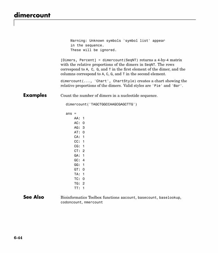
dimercount
Warning: Unknown symbols 'symbol list' appearin the sequence.These will be ignored.
[Dimers, Percent] = dimercount(SeqNT) returns a 4-by-4 matrixwith the relative proportions of the dimers in SeqNT. The rowscorrespond to A, C, G, and T in the first element of the dimer, and thecolumns correspond to A, C, G, and T in the second element.
dimercount(..., 'Chart', ChartStyle) creates a chart showing therelative proportions of the dimers. Valid styles are 'Pie' and 'Bar'.
Examples Count the number of dimers in a nucleotide sequence.
dimercount('TAGCTGGCCAAGCGAGCTTG')
ans =AA: 1AC: 0AG: 3AT: 0CA: 1CC: 1CG: 1CT: 2GA: 1GC: 4GG: 1GT: 0TA: 1TC: 0TG: 2TT: 1
See Also Bioinformatics Toolbox functions aacount, basecount, baselookup,codoncount, nmercount
6-44

dna2rna
Purpose Convert a DNA sequence to an RNA sequence
Syntax SeqRNA = dna2rna(SeqDNA)
ArgumentsSeqDNA DNA sequence. Enter either a character string with the
characters A, T, G, C, and ambiguous characters R, Y, K,M, S, W, B, D, H, V, N, or a vector of integers from the tableMapping Nucleotide Letters to Integers on page 6-143.You can also enter a structure with the field Sequence.
SeqRNA RNA sequence.
Description SeqRNA = dna2rna(SeqDNA) converts a DNA sequence to an RNAsequence by converting any thymine nucleotides (T) in the DNAsequence to uracil (U). The RNA sequence is returned in the sameformat as the DNA sequence. For example, if SeqDNA is a vector ofintegers, then so is SeqRNA.
Examples Convert a DNA sequence to an RNA sequence.
rna = dna2rna('ACGATGAGTCATGCTT')
rna =ACGAUGAGUCAUGCUU
See Also Bioinformatics Toolbox function rna2dna
MATLAB functions regexp, strrep
6-45

emblread
Purpose Read data from an EMBL file
Syntax EMBLData = emblread('File','PropertyName', PropertyValue)
emblread(..., 'SequenceOnly', SequenceOnlyValue)
ArgumentsFile EMBL formatted file (ASCII text file).
Enter a filename, a path and filename, ora URL pointing to a file. File can also bea MATLAB character array that containsthe text for a filename.
SequenceOnlyValue Property to control reading only thesequence. Enter true.
EMBLData MATLAB structure with fieldscorresponding to EMBL data.
EMBLSeq MATLAB character string withoutmetadata for the sequence.
Description EMBLData = emblread('File', 'PropertyName', PropertyValue)reads data from an EMBL formatted file (File) and creates aMATLAB structure (EMBLData) with fields corresponding to the EMBLtwo-character line type code. Each line type code is stored as a separateelement in the structure.
EMBLData for the 137.0 version contains the following fields:
CommentsIdentificationAccessionSequenceVersionDatecreatedDateupdatedDescriptionKeyword
6-46

emblread
OrganismSpeciesOorganismClassificationOrganelleReference.NumberReference.CommentReference.PositionReference{#}.MedLineReferemce{#}.PubMedReference.AuthorsReference.TitleReference.LocationDatabaseCrossReferenceFeatureBasecountSequence
Seq = emblread('File', 'SequenceOnly', SequenceOnlyValue),when SequenceOnly is true, reads only the sequence information .
Examples Get sequence information from the web, save to a file, and then readback into MATLAB.
getembl('X00558','ToFile','rat_protein.txt');EMBLData = emblread('rat_protein.txt')
See Also Bioinformatics Toolbox functions getembl, fastaread, genbankread,genpeptread, pirread, pdbread
6-47

exprprofrange
Purpose Calculate the range of gene expression profiles
Syntax exprprofrange(Data, 'PropertyName', PropertyValue)[Range, LogRange] = exprprofrange(Data)
exprprofrange(..., 'ShowHist', ShowHistValue)
ArgumentsData Matrix where each row corresponds to a gene.
ShowHistValue Property to control the display of a histogramwith range data. Enter true.
Description exprprofrange(Data, 'PropertyName', PropertyValue) calculatesthe range of each expression profile in a dataset (Data).
[Range, LogRange] = exprprofrange(Data) returns the log range,that is, log(max(prof))- log(min(prof)), of each expression profile.If you do not specify output arguments, exprprofrange displays ahistogram bar plot of the range.
exprprofrange(..., 'ShowHist', ShowHistValue), when ShowHist istrue, displays a histogram of the range data .
Examples Calculate the range of expression profiles for yeast data as geneexpression changes during the metabolic shift from fermentation torespiration.
load yeastdatarange = exprprofrange(yeastvalues,'ShowHist',true);
See Also Bioinformatics Toolbox function generangefilter
6-48

exprprofvar
Purpose Calculate the variance of gene expression profiles
Syntax exprprofvar(Data, 'PropertyName', PropertyValue)
exprprofvar(..., 'ShowHist', ShowHistValue)
ArgumentsData Matrix where each row corresponds to a gene.
ShowHistValue Property to control the display of a histogramwith variance data. Enter true.
Description exprprofvar(Data, 'PropertyName', PropertyValue) calculates thevariance of each expression profile in a dataset (Data). If you do notspecify output arguments, this function displays a histogram bar plotof the range.
exprprofvar(..., 'ShowHist', ShowHistValue), when ShowHist istrue, displays a histogram of the range data .
Examples Calculate the variance of expression profiles for yeast data as geneexpression changes during the metabolic shift from fermentation torespiration.
load yeastdatadatavar = exprprofvar(yeastvalues,'ShowHist',true);
See Also Bioinformatics Toolbox functions exprprofrange, generangefilter,genevarfilter
6-49

fastaread
Purpose Read data from a FASTA formatted file
Syntax FASTAData = fastaread('File')[Header, Sequence] = fastaread('File')
ArgumentsFile FASTA formatted file (ASCII text file). Enter a
filename, a path and filename, or a URL pointing to afile. File can also be a MATLAB character array thatcontains the text for a filename.
FASTAData MATLAB structure with the fields Header andSequence.
Description fastaread reads data from a FASTA formatted file into a MATLABstructure with the following fields:
HeaderSequence
A file with a FASTA format begins with a right angle bracket (>) and asingle line description. Following this description is the sequence as aseries of lines with fewer than 80 characters. Sequences are expected touse the standard IUB/IUPAC amino acid and nucleotide letter codes.
For a list of codes, see aminolookup and baselookup.
FASTAData = fastaread('File') reads a file with a FASTA formatand returns the data in a structure. FASTAData.Header is the headerinformation, while FASTAData.Sequence is the sequence stored as astring of letters.
[Header, Sequence] = fastaread('File') reads data from a fileinto separate variables. If the file contains more than one sequence,then header and sequence are cell arrays of header and sequenceinformation.
6-50

fastaread
Examples Get a FASTA formatted sequence from GenBank, save it, and then readthe FASTA file into the MATLAB workspace as a structure.
s= fastaread('p53nt.txt')
s =Header: [1x94 char]Sequence: [1x2629 char]
See Also Bioinformatics Toolbox function aminolookup, baselookup, fastawrite
6-51

fastawrite
Purpose Write to a file using a FASTA format
Syntax fastawrite('File', Data)fastawrite('File', Header, Sequence)
ArgumentsFile Enter either a filename or a path and filename
supported by your operating system. (ASCII textfile).
Data Enter a character string with a FASTA format, asequence object, a structure containing the fieldsSequence and Header, or a GenBank/GenPeptstructure.
Header Information about the sequence.
Sequence Nucleotide or amino acid sequence using thestandard IUB/IUPAC codes. For a list of validcharacters, see and Mapping Nucleotide Letters toIntegers on page 6-143.
Description fastawrite('File', Data) writes the contents of Data to a file with aFASTA format.
fastawrite('File', Header, Sequence) writes header and sequenceinformation to a file with a FASTA format.
Examples %get the sequence for the human p53 gene from GenBank.seq = getgenbank('NM_000546')
%find the CDS line in the FEATURES information.cdsline = strmatch('CDS',seq.Features)
%read the coordinates of the coding region.[start,stop] = strread(seq.Features(cdsline,:),'%*s%d..%d')
%extract the coding region.
6-52

fastawrite
codingSeq = seq.Sequence(start:stop)
%write just the coding region to a FASTA file.fastawrite('p53coding.txt','Coding region for p53',codingSeq);
Save multiple sequences.
data(1).Sequence = 'ACACAGGAAA'data(1).Header = 'First sequence'data(2).Sequence = 'ACGTCAGGTC'data(2).Header = 'Second sequence'
fastawrite('my_sequences.txt', data)type('my_sequences.txt')
>First sequenceACACAGGAAA
>Second sequenceACGTCAGGTC
See Also Bioinformatics Toolbox function fastaread
6-53

galread
Purpose Read microarray data from a GenePix array list file
Syntax GALData = galread('File')
ArgumentsFile GenePix Array List formatted file (GAL). Enter a filename,
or enter a path and filename.
Description galread reads data from a GenePix formatted file into a MATLABstructure.
GALData = galread('File') reads in a GenePix Array List formattedfile (File ) and creates a structure (GALData) containing the followingfields:
HeaderBlockDataIDsNames
The field BlockData is an N-by-3 array. The columns of this array arethe block data, the column data, and the row data respectively. Formore information on the GAL format, see
http://www.axon.com/GN_GenePix_File_Formats.html#gal
For a list of supported file format versions, see
http://www.axon.com/gn_GPR_Format_History.html
GenePix is a registered trademark of Axon Instruments, Inc.
See Also Bioinformatics Toolbox functions gprread, maimage, sptread
6-54

genbankread
Purpose Read data from a GenBank file
Syntax GenBankData = genbankread('File')
ArgumentsFile GenBank formatted file (ASCII text file). Enter a
filename, a path and filename, or a URL pointing toa file. File can also be a MATLAB character arraythat contains the text of a GenBank formatted file.
GenBankData MATLAB structure with fields corresponding toGenBank data.
Discussion genbankread reads data from a GenBank formatted file into a MATLABstructure.
GenBankData = genbankread('File') reads in a GenBank formattedfile (File) and creates a structure (Data) containing fields correspondingto the GenBank keywords. Each separate sequence listed in theoutput structure (GenBankData) is stored as a separate element of thestructure.
GenBankData contains the following fields:
LocusNameLocusSequenceLengthLocusMoleculeTypeLocusGenBankDivisionLocusModificationDateDefinitionAccessionVersionGIKeywordsSegmentSourceSourceOrganismReference.Number
6-55
genbankread
Reference.AuthorsReference.TitleReference.JournalReference.MedLineReference.PubMedReference.RemarkCommentFeaturesBaseCountSequence
Examples Get sequence information for the gene HEXA, store in a file, and thenread back into MATLAB.
getgenbank('nm_000520', 'ToFile', 'TaySachs_Gene.txt')s = genbankread('TaySachs_Gene.txt')
See Also Bioinformatics Toolbox functions emblread, getgenbank, fastaread,genpeptread, getgenbank, scfread
6-56

geneentropyfilter
Purpose Remove genes with low entropy expression values
Syntax Mask = geneentropyfilter(Data,'PropertyName', PropertyValue)[Mask, FData] = geneentropyfilter(Data)[Mask, FData, FNames] = geneentropyfilter(Data, Names)
geneentropyfilter(..., 'Prctile', PrctileValue)
ArgumentsData Matrix where each row corresponds to the
experimental results for one gene. Each column isthe results for all genes from one experiment.
Names Cell array with the same number of rows as Data.Each row contains the name or ID of the gene inthe data set.
PrctileValue Property to specify a percentile below which genedata is removed. Enter a value from 0 to 100.
Description Mask = geneentropyfilter(Data, 'PropertyName', PropertyValue)identifies gene expression profiles in Data with entropy values less thanthe 10th percentile.
Mask is a logical vector with one element for each row in Data. Theelements of Mask corresponding to rows with a variance greater thanthe threshold have a value of 1, and those with a variance less thenthe threshold are 0.
[Maks, FData] = geneentropyfilter(Data) returns a filtereddata matrix (FData). FData can also be created using FData =Data(find(I),:).
[Mask, FData,FNames] = geneentropyfilter(Data, Names) returnsa filtered names array (FNames), where Names is a cell array of thenames of the genes corresponding to each row of Data. FNames can alsobe created using FNames = Names(I).
6-57

geneentropyfilter
geneentropyfilter(..., 'Prctile', PrctileValue) removes fromData gene expression profiles with entropy values less than thepercentile Prctile.
Examples load yeastdata[fyeastvalues, fgenes] = geneentropyfilter(yeastvalues,genes);
See Also Bioinformatics Toolbox functions exprprofrange, exprprofvar,genelowvalfilter, generangefilter
6-58

genelowvalfilter
Purpose Remove gene profiles with low absolute values
Syntax Mask = genelowvalfilter(Data, 'PropertyName', PropertyValue)[Mask, FData] = genelowvalfilter(Data)[Mask, FData, FNames] = genelowvalfilter(Data, Names)
genelowvalfilter(..., 'Prctile', PrctileValue)genelowvalfilter(..., 'AbsValue', AbsValueValue)genelowvalfilter(..., 'AnyVal', AnyValValue)
ArgumentsData Matrix where each row corresponds to the
experimental results for one gene. Each column isthe results for all genes from one experiment.
Names Cell array with the same number of rows as Data.Each row contains the name or ID of the gene inthe data set.
PrctileValue Property to specify a percentile below which geneexpression profiles are removed. Enter a valuefrom 0 to 100.
AbsValueValue Property to specify an absolute value below whichgene expression profiles are removed.
AnyValValue Property to select the minimum or maximumabsolute value for comparison with AbsValue.If AnyValValue is true, selects the minimumabsolute value. If AnyVal is false, selects themaximum absolute value. The default value isfalse.
Description Gene expression profile experiments have data where the absolutevalues are very low. The quality of this type of data is often bad due tolarge quantization errors or simply poor spot hybridization.
6-59

genelowvalfilter
Mask = genelowvalfilter(Data, 'PropertyName', PropertyValue)identifies gene expression profiles in Data with all absolute values lessthan the 10th percentile.
Mask is a logical vector with one element for each row in Data. Theelements of Mask corresponding to rows with absolute expression levelsgreater than the threshold have a value of 1, and those with absoluteexpression levels less then the threshold are 0.
[Mask, FData] = genelowvalfilter(Data) returns a filtereddata matrix (FData). FData can also be created using FData =Data(find(I),:).
[Mask, FData,FNames] = genelowvalfilter(Data, Names) returns afiltered names array (FNames), where Names is a cell array of the namesof the genes corresponding to each row of Data. FNames can also becreated using FNames = Names(I).
genelowvalfilter(..., 'Prctile', PrctileValue) removes fromData gene expression profiles with all absolute values less than thepercentile Prctile.
genelowvalfilter(..., 'AbsValue', AbsValueValue) calculates themaximum absolute value for each gene expression profile and removesthe profiles with maximum absolute values less than AbsVal.
genelowvalfilter(..., 'AnyVal', AnyValValue), when AnyVal istrue, calculates the minimum absolute value for each gene expressionprofile and removes the profiles with minimum absolute values lessthan AnyVal.
Examples [data, labels, I, FI] = genelowvalfilter(data,labels,'AbsValue',5);
See Also Bioinformatics Toolbox functions exprprofrange, exprprofvar,geneentropyfilter, generangefilter
6-60

generangefilter
Purpose Remove gene profiles with small profile ranges
Syntax Mask = generangefilter(Data, 'PropertyName', PropertyValue)[Mask, FData] generangefilter(Data)[Mask, FData, FNames] = generangefilter(Data, Names)
generangefilter(..., 'Prctile', PrctileValue)generangefilter(..., 'AbsValue', AbsValueValue)generangefilter(..., 'LOGPrctile', LOGPrctileValue)generangefilter(..., 'LOGValue', LOGValueValue)
ArgumentsData Matrix where each row corresponds to the
experimental results for one gene. Eachcolumn is the results for all genes from oneexperiment.
Names Cell array with the same number of rows asData. Each row contains the name or ID of thegene in the data set.
PrctileValue Property to specify a percentile below whichgene expression profiles are removed. Entera value from 0 to 100.
AbsValueValue Property to specify an absolute value belowwhich gene expression profiles are removed.
LOGPrctileValue Property to specify the LOG of a percentile.
LOGValueValue Property to specify the LOG of an absolutevalue.
Description Mask = generangefilter(Data, 'PropertyName', PropertyValue)calculates the range for each gene expression profile in Data, andthen identifies the expression profiles with ranges less than the 10thpercentile.
6-61

generangefilter
Mask is a logical vector with one element for each row in Data. Theelements of Mask corresponding to rows with a range greater thenthe threshold have a value of 1, and those with a range less then thethreshold are 0.
[Maks, FData] = generangefilter(Data) returns a filtereddata matrix (FData). FData can alos be created using FData =Data(find(I),:).
[Maks, FData, FNames] = generangefilter(Data, Names) returns afiltered names array (FNames), where Names is a cell array of the namesof the genes corresponding to each row of Data. FNames can also becreated using FNames = Names(I).
generangefilter(..., 'Prctile', PrctileValue) removes fromData gene expression profiles with ranges less than the percentilePrctile.
generangefilter(..., 'AbsValue', AbsValueValue) removes fromData gene expression profiles with ranges less than AbsValue.
generangefilter(..., 'LOGPrctile', LOGPrctileValue) filtersgenes with profile ranges in the lowest LOGPrctile percent of the logrange.
generangefilter(..., 'LOGValue', LOGValueValue) filters geneswith profile log ranges lower than LOGValue.
Examples load yeastdata[mask, fyeastvalues, fgenes] = generangefilter(yeastvalues,genes);
See Also Bioinformatics Toolbox functions exprprofrange, geneentropyfilter,genelowvalfilter, genevarfilter
6-62
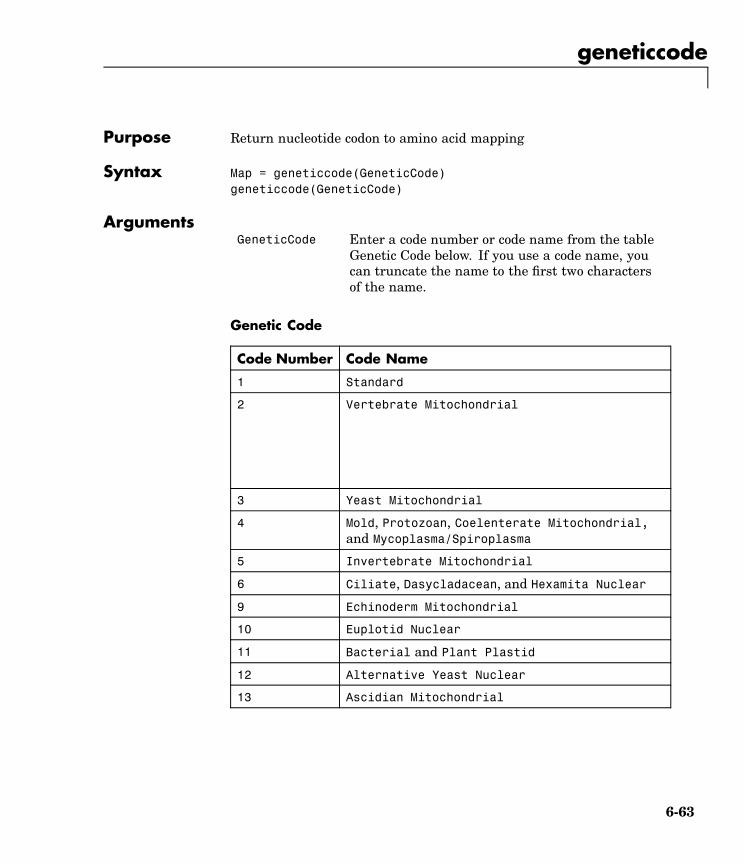
geneticcode
Purpose Return nucleotide codon to amino acid mapping
Syntax Map = geneticcode(GeneticCode)geneticcode(GeneticCode)
ArgumentsGeneticCode Enter a code number or code name from the table
Genetic Code below. If you use a code name, youcan truncate the name to the first two charactersof the name.
Genetic Code
Code Number Code Name
1 Standard
2 Vertebrate Mitochondrial
3 Yeast Mitochondrial
4 Mold, Protozoan, Coelenterate Mitochondrial,and Mycoplasma/Spiroplasma
5 Invertebrate Mitochondrial
6 Ciliate, Dasycladacean, and Hexamita Nuclear
9 Echinoderm Mitochondrial
10 Euplotid Nuclear
11 Bacterial and Plant Plastid
12 Alternative Yeast Nuclear
13 Ascidian Mitochondrial
6-63

geneticcode
Code Number Code Name
14 Flatworm Mitochondrial
15 Blepharisma Nuclear
16 Chlorophycean Mitochondrial
21 Trematode Mitochondrial
22 Scenedesmus Obliquus Mitochondrial
23 Thraustochytrium Mitochondrial
Description Map = geneticcode returns a structure with a mapping of nucleotidecodons to amino acids for the standard genetic code.
geneticcode(GeneticCode)returns a structure of the mappingfor alternate genetic codes, where GeneticCode is either thetransl_table (code) number from the NCBI Genetics web page(http://www.ncbi.nlm.nih.gov/Taxonomy/Utils/wprintgc.cgi?mode=c)or one of the supported names in the genetic code table above.
Examples List the mapping of nucleotide codons to amino acids for a specificgenetic code.
wormcode = geneticcode('Flatworm Mitochondrial');
See Also Bioinformatics Toolbox functions aa2nt, baselookup, nt2aa,revgeneticcode, seqshoworfs
6-64

genevarfilter
Purpose Filter genes with small profile variance
Syntax Mask = genevarfilter(Data, 'PropertyName', PropertyValue)[Mask, FData] = genevarfilter(Data)[Mask, FData, FNames] = genevarfilter(Data, Names)
genevarfilter(..., 'Prctile', PrctileValue)genevarfilter(..., 'AbsValue', AbsValueValue)
ArgumentsData Matrix where each row corresponds to a gene.
The first column is the name of the genes, andeach additional column is the results from anexperiment.
Names Cell array with the same number of rows as Data.Each row contains the name or ID of the genein the data set.
PrctileValue Property to specify a percentile below which geneexpression profiles are removed. Enter a valuefrom 0 to 100
AbsValueValue Property to specify an absolute value belowwhich gene expression profiles are removed.
Description Gene profiling experiments have genes which exhibit little variationin the profile and are generally not of interest in the experiment.Removing (filtering) these genes from the data is a commonly done.
Mask = genevarfilter(Data, 'PropertyName', PropertyValue)calculates the variance for each gene expression profile in Data andthen identifies the expression profiles with a variance less than the10th percentile.
Mask is a logical vector with one element for each row in Data. Theelements of Mask corresponding to rows with a variance greater thenthe threshold have a value of 1, and those with a variance less thenthe threshold are 0.
6-65

genevarfilter
[Mask, FData] = genevarfilter(Data) returns the filtereddata matrix FData. FData can also be created using FData =Data(find(I),:).
[Mask, FData, FNames] = genevarfilter(Data, Names) returns afiltered names array (FNames). Names is a cell array of the names of thegenes corresponding to each row of Data. FNames can also be createdusing FNames = Names(I).
genevarfilter(..., 'Prctile', PrctileValue) removes from Datagene expression profiles with a variance less than the percentilePrctile.
genevarfilter(..., 'AbsValue', AbsValValue) removes from Datagene expression profiles with a variance less than AbsValue.
Examples load yeastdata[fyeastvalues, fgenes] = genevarfilter(yeastvalues,genes);
See Also Bioinformatics Toolbox functions exprprofrange, exprprofvar,generangefilter
6-66

genpeptread
Purpose Read data from a GenPept file
Syntax GenPeptData = genpeptread('File')
ArgumentsFile GenPept formatted file (ASCII text file). Enter a
filename, a path and filename, or a URL pointing to afile. File can also be a MATLAB character array thatcontains the text of a GenPept file.
Description genpeptread reads data from a GenPept formatted file into a MATLABstructure.
Note NCBI has recently changed the name of their protein searchengine from GenPept to Entrez Protein. However, the function namesin the Bioinformatics Toolbox (getgenpept, genpeptread) are unchangedrepresenting the still-used GenPept report format.
GenPeptData = genpeptread('File') reads in the GenPept formattedsequence from File and creates a structure GenPeptData, containingfields corresponding to the GenPept keywords. Each separate sequencelisted in File is stored as a separate element of the structure.GenPeptDATA contains these fields:
LocusNameLocusSequenceLengthLocusMoleculeTypeLocusGenBankDivisionLocusModificationDateDefinitionAccessionPIDVersionGI
6-67

genpeptread
DBSourceKeywordsSourceSourceDatabaseSourceOrganismReference.NumberReference.AuthorsReference.TitleReference.JournalReference.MedLineReference.PubMedReference.RemarkCommentFeaturesWeightLengthSequence
Examples Get sequence information for the protein coded by the gene HEXA, saveto a file, and then read back into MATLAB.
getgenpept('p06865', 'ToFile', 'TaySachs_Protein.txt')genpeptread('TaySachs_Protein.txt')
See Also Bioinformatics Toolbox functions fastaread, genbankread, getgenpept,pdbread, pirread
6-68

geosoftread
Purpose Read data from a Gene Expression Omnibus (GEO) SOFT file
Syntax GEOSOFTData = geosoftread('File')
ArgumentsFile Gene Expression Omnibus (GEO) formatted file (ASCII
text file). Enter a filename, a path and filename, or aURL pointing to a file. File can also be a MATLABcharacter array that contains the text of a GEO file.
Description geosoftread reads data from a Gene Expression Omnibus (GEO) SOFTformatted file (File), and creates a MATLAB structure (GEOSOFTdata)with the following fields:
ScopeAccessionHeaderColumnDescriptionsColumnNamesData
Fields correspond to the GenBank keywords. Each separate entry listedin File is stored as a separate element of the structure.
Examples Get data from the GEO web site and save it to a file.
geodata = getgeodata('GSM3258','ToFile','GSM3258.txt');
Use geosoftread to access a local copy from disk instead of accessingit from the GEO web site.
geodata = geosoftread('GSM3258.txt')
See Also Bioinformatics Toolbox functions galread, getgeodata, gprread,sptread
6-69

get (phytree)
Purpose Get information about a phylogenetic tree object
Syntax [Value1,Value2, ...] = GET(Tree,'Name1', 'Name2', ...)
ArgumentsTree Phytree object created with the function
phytree.
Name Property name for a phytree object.
Description [Value1,Value2, ...] = GET(Tree, 'Name1', 'Name2', ...)returns the specified properties from a phytree object (Tree).
The valid choices for 'Name' are
'Pointers' Branch to leaf/branch connectivity list
'Distances' Edge length for every leaf/branch
'NumLeaves' Number of leaves
'NumBranches' Number of branches
'NumNodes' Number of nodes (NumLeaves +Numbranches)
'LeafNames' Names of the leaves
'BranchNames' Names of the branches
'NodeNames' Names of all the nodes
Examples tr = phytreeread('pf00002.tree')protein_names = get(tr,'LeafNames')
See Also Bioinformatics Toolbox functions phytree, phytreeread, and phytreeobject method select
6-70

getblast
Purpose Get BLAST report from NCBI web site
Syntax Data = getblast(RID)
getblast(..., 'Descriptions', DescriptionsValue)getblast(..., 'Alignments', AlignmentsValue)getblast(..., 'ToFile', ToFileValue)getblast(..., 'FileFormat', FileFormatValue)
ArgumentsRID BLAST Request ID (RID) from the
function blastncbi.
DescriptionsValue Property to select the number ofdescriptions in a report. Enter a numberfrom 1 to 100. The default value is 100.
AlignmentsValue Property to select the number ofalignments in a report. Enter values from1 to 100. The default value is 50.
ToFileValue Property to enter a filename for savingreport data.
FileFormatValue Property to select the format of the filenamed in ToFileValue. Enter either'TEXT' or ’HTML’.The default value is'TEXT'.
Description BLAST (Basic Local Alignment Search Tool) reports offer a fast andpowerful comparative analysis of interesting protein and nucleotidesequences against known structures in existing online databases.getblast parses NCBI BLAST reports, including BLASTN, BLASTP,BLASTX, TBLASTN, TBLASTX and psi-BLAST.
6-71

getblast
Data = getblast(RID) reads a BLAST Request ID (RID) and returnsthe report data in a structure (Data). The NCBI Request ID (RID) mustbe a recently generated report because NCBI purges reports after 24hours.
getblast(..., 'Descriptions', DescriptionsValue) includes thespecified number of descriptions (DescriptionsValue) in the report.
getblast(..., 'Alignments', AlignmentsValue) includes thespecified number of alignments in the report.
getblast(..., 'ToFile', ToFileValue) saves the data returned fromthe NCBI BLAST report to a file (ToFileValue). The default format forthe file is text, but you can specify HTML with the property FileFormat.
getblast(..., 'FileFormat', FileFormatValue) returns the reportin the specified format (FileFormatValue).
For more information about reading and interpreting BLAST reports,see
http://www.ncbi.nlm.nih.gov/Education/BLASTinfo/Blast_output.html
Examples Run a BLAST search with an NCBI accession number.RID = blastncbi('AAA59174','blastp','expect',1e-10)
% Then pass the RID to GETBLAST to parse the report, load it into% a MATLAB structure, and save a copy as a text file.report = getblast(RID,'TOFILE','Report.txt')
See Also Bioinformatics Toolbox functions blastncbi, blastread
6-72

getbyname (phytree)
Purpose Select branches and leaves by name from a phytree object
Syntax S = getbyname(Tree, Expression)
ArgumentsTree Phytree object created with the function
phytree.
Expression Regular expression.
Description S = getbyname(Tree, Expression) returns a logical vector (S) of sizeNumNodes-by-1 with the node names of a phylogenetic tree (Tree) thatmatch the regular expression (Expression) regardless of letter case.When Expression is a cell array of strings, getbyname returns a matrixwhere each column corresponds to a query in Expression
For information about the symbols that you can use in a matchingregular expression, see the MATLAB function regexp.
Examples % Load a phylogenetic tree created from a protein family:tr = phytreeread('pf00002.tree');
% Select all the 'mouse' and 'human' proteins:sel = getbyname(tr,{'mouse','human'});view(tr,any(sel,2));
See Also The MATLAB function regexp
6-73
getembl
Purpose Retrieve sequence information from the EMBL database
Syntax Data = getembl('AccessionNumber','PropertyName', PropertyValue)
getembl(..., 'ToFile', ToFileValue)getembl(..., 'SequenceOnly', SequenceOnlyValue)
ArgumentsAccessionNumber Unique identifier for a sequence record. Enter a
unique combination of letters and numbers
ToFileValue Property to specify the location and filenamefor saving data. Enter either a filename or apath and filename supported by your system(ASCII text file).
SequenceOnlyValue Property to control getting a sequence withoutthe metadata. Enter true or false.
Description getembl retrieves information from the European Molecular BiologyLaboratory (EMBL) database for nucleotide sequences. This database ismaintained by the European Bioinformatics Institute (EBI). For moredetails about the EMBL-Bank database, see
http://www.ebi.ac.uk/embl/Documentation/index.html
Data = getembl('AccessionNumber', 'PropertyName',PropertyValue) searches for the accession number in the EMBLdatabase (http://www.ebi.ac.uk/embl) and returns a MATLABstructure containing the following fields:
CommentsIdentificationAccessionSequenceVersionDateCreatedDateUpdated
6-74

getembl
DescriptionKeywordOrganismSpeciesOrganismClassificationOrganelleReferenceDatabaseCrossReferenceFeatureBaseCountSequence
getembl(..., 'ToFile', ToFileValue) returns a structure containinginformation about the sequence and saves the information in a fileusing an EMBL data format. If you do not give a location or path to thefile, the file is stored in the MATLAB current directory. Read an EMBLformatted file back into MATLAB using the function emblread.
getembl(..., 'SequenceOnly', SequenceOnlyValue) if SequenceOnlyis true, returns only the sequence information without the metadata.
Examples Retrieve data for the rat liver apolipoprotein A-I.
emblout = getembl('X00558')
Retrieve data for the rat liver apolipoprotein and save in the filerat_protein. If a filename is given without a path, the file is stored inthe current directory.
Seq = getembl('X00558','ToFile','c:\project\rat_protein.txt')
Retrieve only the sequence for the rat liver apolipoprotein.
Seq = getembl('X00558','SequenceOnly',true)
See Also Bioinformatics Toolbox functions emblread, getgenbank, getgenpept,getpdb, getpir
6-75

getgenbank
Purpose Retrieve sequence information from the GenBank database
Syntax Data = getgenbank('AccessionNumber','PropertyName',PropertyValue)
getgenbank(..., 'ToFile', ToFileValue)getgenbank(..., 'FileFormat', FileFormatValue)getgenbank(..., 'SequenceOnly', SequenceOnlyValue)
ArgumentsAccessionNumber Unique identifier for a sequence record.
Enter a unique combination of letters andnumbers.
ToFileValue Property to specify the location and filenamefor saving data. Enter either a filename or apath and filename supported by your system(ASCII text file).
FileFormatValue Property to select the format for the filespecified with the property ToFileValue.Enter either 'GenBank' or 'FASTA'.
SequenceOnlyValue Property to control getting the sequence only.Enter either true or false.
Description getgenbank retrieves nucleotide and amino acid sequence informationfrom the GenBank database. This database is maintained by theNational Center for Biotechnology Information (NCBI). For more detailsabout the GenBank database, see
http://www.ncbi.nlm.nih.gov/Genbank/
Data = getgenbank('AccessionNumber', 'PropertyName',PropertyValue) searches for the accession number in the GenBankdatabase and returns a MATLAB structure containing informationfor the sequence. If an error occurs while retrieving the GenBank
6-76

getgenbank
formatted information, then an attempt is make to retrieve the FASTAformatted data.
getgenbank(..., 'ToFile', ToFileValue) saves the data returnedfrom GenBank in a file. If you do not give a location or path to the file,the file is stored in the MATLAB current directory. Read a GenBankformatted file back into MATLAB using the function genbankread.
getgenbank(..., 'FileFormat', FileFormatValue) returns thesequence in the specified format FileFormatValue.
getgenbank(..., 'SequenceOnly', SequenceOnlyValue) whenSequenceOnly is true, returns only the sequence as a character array.When the properties SequenceOnly and ToFile are used together, theoutput file is in the FASTA format.
getgenbank(...) displays the information to the screen without returningdata to a variable. The displayed information includes hyperlinks to theURLS used to search for and retrieve the data.
Examples Retrieve the sequence from chromosome 19 that codes for the humaninsulin receptor and store it in structure S.
S = getgenbank('M10051')
S =
LocusName: 'HUMINSR'LocusSequenceLength: '4723'LocusNumberofStrands: ''
LocusTopology: 'linear'LocusMoleculeType: 'mRNA'
LocusGenBankDivision: 'PRI'LocusModificationDate: '06-JAN-1995'
Definition: 'Human insulin receptor mRNA, complete cdsAccession: 'M10051'
Version: 'M10051.1'GI: '186439'
Keywords: 'insulin receptor; tyrosine kinase.'
6-77

getgenbank
Segment: []Source: 'Homo sapiens (human)'
SourceOrganism: [3x65 char]Reference: {[1x1 struct]}
Comment: [14x67 char]Features: [51x74 char]
CDS: [139 4287]Sequence: [1x4723 char]
SearchURL: [1x10⁵ char]RetrieveURL: [1x95 char]
See Also Bioinformatics Toolbox functions genbankread, getembl, getgenpept,getpdb, getpir
6-78

getgenpept
Purpose Retrieve sequence information from the GenPept database
Syntax Data = getgenpept('AccessionNumber','PropertyName', PropertyValue)
getgenpept(..., 'ToFile', ToFileValue)getgenpept(..., 'SequenceOnly', SequenceOnlyValue)
ArgumentsAccessionNumber Unique identifier for a sequence record.
Enter a combination of letters andnumbers.
ToFileValue Property to specify the location andfilename for saving data. Enter either afilename or a path and filename supportedby your system (ASCII text file).
FileFormatValue Property to select the format for the filespecified with the property ToFileValue.Enter either 'GenBank' or 'FASTA'.
SequenceOnlyValue Property to control getting the sequenceonly. Enter either true or false.
Description getgenpept retrieves a protein (amino acid) sequence and sequenceinformation from the database GenPept. This database is a translationof the nucleotide sequences in GenBank and is maintained by theNational Center for Biotechnology Information (NCBI).
Note NCBI has recently changed the name of their protein searchengine from GenPept to Entrez Protein. However, the function namesin the Bioinformatics Toolbox (getgenpept, genpeptread) are unchangedrepresenting the still-used GenPept report format.
6-79

getgenpept
For more details about the GenBank database, see
http://www.ncbi.nlm.nih.gov/Genbank/
Data = getgenpept('AccessionNumber','PropertyName',PropertyValue) searches for theaccession number in the GenPept database and returns a MATLABstructure containing for the sequence. If an error occurs whileretrieving the GenBank formatted information, then an attempt ismake to retrieve the FASTA formatted data.
getgenpept(..., 'ToFile', ToFileValue) saves the information ina file. If you do not give a location or path to the file, the file is storedin the MATLAB current directory. Read a GenPept formatted file backinto MATLAB using the function genpeptread
getgenpept(..., 'FileFormat', FileFormatValue) returns thesequence in the specified format FileFormatValue.
getgenpept(..., 'SequenceOnly', SequenceOnlyValue) returns onlythe sequence information without the metadata if SequenceOnly istrue. When the properties SequenceOnly and ToFile are used together,the output file is in the FASTA format.
getgenpept(...) displays the information to the screen withoutreturning data to a variable. The displayed information includeshyperlinks to the URLs used to search for and retrieve the data.
Examples Retrieve the sequence for the human insulin receptor and store it instructure Seq.
Seq = getgenpept('AAA59174')
See Also Bioinformatics Toolbox functions genpeptread, getembl, getgenbank,getpdb, getpir
6-80

getgeodata
Purpose Get Gene Expression Omnibus (GEO) data
Syntax Data = getgeodata('AccessionNumber''PropertyName', PropertyValue)
getgeodata(..., 'ToFile', ToFileValue)
ArgumentsAccessionNumber Unique identifier for a sequence record. Enter
a combination of letters and numbers.
ToFileValue Property to specify the location and filenamefor saving data. Enter either a filename, or apath and filename supported by your system(ASCII text file).
Description Data = getgeodata('AccessionNumber','PropertyName',PropertyValue) searches for theaccession number in the Gene Expression Omnibus database andreturns a MATLAB structure containing the following fields:
ScopeAccessionHeaderColumnDescriptionsColumnNamesData
getgeodata(..., 'ToFile', ToFileValue) saves the data returnedfrom the database to a file. Read a GenPept formatted file back intoMATLAB using the function gensoftread.
For more information, see
http://www.ncbi.nlm.nih.gov/About/disclaimer.html
6-81

getgeodata
Examples geoStruct = getgeodata('GSM1768')
See Also Bioinformatics Toolbox functions geosoftread, getgenbank, getgenpept
6-82

gethmmalignment
Purpose Retrieve multiple aligned sequences from the PFAM database
Syntax ‘AlignData = gethmmalignment('PFAMKey',
'PropertyName', PropertyValue)
gethmmalignment(..., 'ToFile', ToFileValue)gethmmalignment(..., 'Type', TypeValue)
ArgumentsPFAMKey Unique identifier for a sequence record. Enter a
unique combination of letters and numbers.
ToFileValue Property to specify the location and filename forsaving data. Enter either a filename, or a path andfilename supported by your system (ASCII text file).
TypeValue Property to select the set of alignments returned.Enter either 'seed' or 'full'.
Description AlignData = gethmmalignment('PFAMKey','PropertyName',PropertyValue) retrieves multiplealigned sequences from a profile hidden Markov model stored in thePFAM database and returns a MATLAB structure containing thefollowing fields:
HeaderSequence
gethmmalignment(..., 'ToFile', ToFileValue) saves the datareturned from the PFAM database to a file. Read a FASTA formattedfile with PFAM data back into MATLAB using the function fastaread.
gethmmalignment(..., 'Type', TypeValue) returns only thealignments used to generate the HMM model if Type='seed', and if
6-83
gethmmalignment
Type='full', returns all alignments that fit the model. Default is'full'.
Examples Retrieve a multiple alignment of the sequences used to train the HMMprofile model for global alignment to the 7 transmembrane receptorprotein in the secretin family (PFAMKey = PF00002).
pfamalign = gethmmalignment(2,'Type','seed')
or
pfamalign = gethmmalignment('PF00002','Type','seed')
See Also Bioinformatics Toolbox function fastaread, gethmmprof, gethmmtree,pfamhmmread
6-84

gethmmprof
Purpose Retrieve profile hidden Markov models from the PFAM database
Syntax Model = gethmmprof('AccessionNumber','PropertyName', PropertyValue)
gethmmprof(..., 'ToFile', ToFileValue)gethmmprof(..., 'Mode', ModeValue)
ArgumentsAccessionNumber Unique identifier for a sequence record. Enter
a unique combination of letters and numbers.
ToFileValue Property to specify the location and filenamefor saving data. Enter either a filename or apath and filename supported by your system(ASCII text file).
ModeValue Property to select returning the global or localalignment mode. Enter either 'ls' for theglobal alignment mode or 'fs' for the localalignment mode. Default value is 'ls'.
Description Model = gethmmprof('AccessionNumber','PropertyName',PropertyValue) searches for the PFAMfamily accession number in the PFAM database and returns a MATLABstructure containing the following fields:
NamePfamAccessionNumberModelDescriptionModelLengthAlphabetMatchEmissionInsertEmissionNullEmissionBeginXMatchX
6-85

gethmmprof
InsertXDeleteXFlankingInsertX
gethmmprof(..., 'ToFile', ToFileValue) saves the data returnedfrom the PFAM database in a file. Read a hmmprof formatted file backinto MATLAB using the function pfamhmmread.
gethmmprof(..., 'Mode', ModeValue) selects either the globalalignment model or the local alignment model.
Examples Retrieve a HMM profile model for global alignment to the 7transmembrane receptor protine in the secretin family. (PFAM key= PF00002)
hmmmodel = gethmmprof(2)
or
hmmmodel = gethmmprof('PF00002')
See Also Bioinformatics Toolbox functions hmmprofalign, hmmprofstruct,pfamhmmread, showhmmprof
6-86

gethmmtree
Purpose Get phylogenetic tree data from PFAM database
Syntax Tree = gethmmtree(AccessionNumber)
Tree = gethmmtree(...,'ToFile',ToFileValue)Tree = gethmmtree(...,'Type', TypeValue)
ArgumentsAccessionNumber Accession number in the PFAM database
ToFileValue Property to specify the location and filenamefor saving data. Enter either a filename or apath and filename supported by your system(ASCII text file).
TypeValue Property to control which alignments areincluded in the tree. Enter either 'seed' or'full'. The default value is 'full'
Description Tree = gethmmtree(AccessionNumber) searches for the PFAM familyaccession number in the PFAM database and returns an object (Tree)containing a phylogenetic tree representative of the protein family.
Tree = gethmmtree(...,'ToFile', ToFileValue) saves the datareturned from the PFAM database in the file ToFileValue.
Tree = gethmmtree(...,'Type', TypeValue), when Type is 'seed',returns a tree with only the alignments used to generate the HMMmodel. When Type is 'full', returns a tree with all of the alignmentsthat hit the model. .
Examples Retrieve a phylogenetic tree built from the multiple aligned sequencesused to train the HMM profile model for global alignment. The PFAMaccession number PF00002 is for the 7-transmembrane receptor proteinin the secretin family.
tree = gethmmtree(2, 'type', 'seed')tree = gethmmtree('PF00002', 'type', 'seed')
6-87

gethmmtree
See Also Bioinformatics Toolbox functions, fastaread, gethmmprof, pfamhmmread
6-88

getpdb
Purpose Retrieve protein structure information from the PDB database
Syntax Data = getpdb('PDBid','PropertyName', PropertyValue)
getpdb(..., 'ToFile', ToFileValue)getpdb(..., 'MirrorSite', MirrorSiteValue)
ArgumentsPDBid Unique identifier for a protein structure
record. Each structure in the PDB isrepresented by a 4-character alphanumericidentifier.
For example, 4hhb is the identification codefor hemoglobin.
ToFileValue Property to specify the location andfilename for saving data. Enter either afilename or a path and filename supportedby your system (ASCII text file).
MirrorSiteValue Property to select Web site. Enter eitherhttp://rutgers.rcsb.org/pdb to usethe Rutgers University Web site, orenter http://nist.rcsb.org/pdb forthe National Institute of Standards andTechnology site.
Description getpdb retrieves sequence information from the Protein Data Bank.This database contains 3-D biological macromolecular structure data.
Data = getpdb('PDBid', 'PropertyName',PropertyValue) searchesfor the ID in the PDB database and returns a MATLAB structurecontaining the following fields:
HeaderTitle
6-89

getpdb
CompoundSourceKeywordsExperimentDataAuthorsJournalRemark1Remark2Remark3SequenceHeterogenNameHeterogenSynonymFormulaSiteAtomRevisionDateSupersededRemark4Remark5HeterogenHelixTurnCryst1OriginXScaleTerminalHeterogenAtomConnectivity
getpdb(..., 'ToFile', ToFileValue) saves the data returned fromthe database to a file. Read a PDB formatted file back into MATLABusing the function pdbread.
getpdb(...,'MirrorSite', MirrorSiteValue) allows you to choosea mirror site for the PDB database. The default site is the SanDiego Supercomputer Center, http://www.rcsb.org/pdb. See
6-90

getpdb
http://www.rcsb.org/pdb/mirrors.html for a full list of PDB mirrorsites.
Examples Retrieve the structure information for the electron transport (hemeprotein) with PDB ID 5CYT.
pdbstruct = getpdb('5CYT')
See Also Bioinformatics Toolbox functions getembl, getgenbank, getgenpept,getpir, pirread
6-91
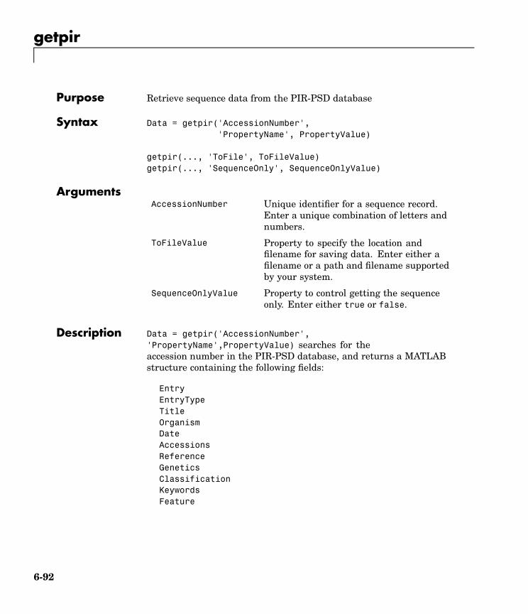
getpir
Purpose Retrieve sequence data from the PIR-PSD database
Syntax Data = getpir('AccessionNumber','PropertyName', PropertyValue)
getpir(..., 'ToFile', ToFileValue)getpir(..., 'SequenceOnly', SequenceOnlyValue)
ArgumentsAccessionNumber Unique identifier for a sequence record.
Enter a unique combination of letters andnumbers.
ToFileValue Property to specify the location andfilename for saving data. Enter either afilename or a path and filename supportedby your system.
SequenceOnlyValue Property to control getting the sequenceonly. Enter either true or false.
Description Data = getpir('AccessionNumber','PropertyName',PropertyValue) searches for theaccession number in the PIR-PSD database, and returns a MATLABstructure containing the following fields:
EntryEntryTypeTitleOrganismDateAccessionsReferenceGeneticsClassificationKeywordsFeature
6-92
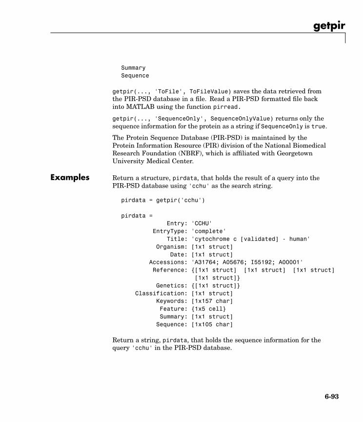
getpir
SummarySequence
getpir(..., 'ToFile', ToFileValue) saves the data retrieved fromthe PIR-PSD database in a file. Read a PIR-PSD formatted file backinto MATLAB using the function pirread.
getpir(..., 'SequenceOnly', SequenceOnlyValue) returns only thesequence information for the protein as a string if SequenceOnly is true.
The Protein Sequence Database (PIR-PSD) is maintained by theProtein Information Resource (PIR) division of the National BiomedicalResearch Foundation (NBRF), which is affiliated with GeorgetownUniversity Medical Center.
Examples Return a structure, pirdata, that holds the result of a query into thePIR-PSD database using 'cchu' as the search string.
pirdata = getpir('cchu')
pirdata =Entry: 'CCHU'
EntryType: 'complete'Title: 'cytochrome c [validated] - human'
Organism: [1x1 struct]Date: [1x1 struct]
Accessions: 'A31764; A05676; I55192; A00001'Reference: {[1x1 struct] [1x1 struct] [1x1 struct]
[1x1 struct]}Genetics: {[1x1 struct]}
Classification: [1x1 struct]Keywords: [1x157 char]Feature: {1x5 cell}Summary: [1x1 struct]
Sequence: [1x10⁵ char]
Return a string, pirdata, that holds the sequence information for thequery 'cchu' in the PIR-PSD database.
6-93

getpir
pirseq = getpir('cchu','SequenceOnly',true)
Return a structure, pirdata, that holds the result of a query into thePIR database using 'cchu' as the search string. It also creates a textfile, cchu.pir, in the current folder that holds the data retrieved fromthe PIR database. Note that the entire data retrieved from the databaseis stored in ToFileValue even if SequenceOnly is true.
pirdata = getpir('cchu', 'ToFile','cchu.pir')
See Also Bioinformatics Toolbox functions genpeptread, getgenpept, getpdb,pdbread, pirread
6-94

gonnet
Purpose Return a Gonnet scoring matrix
Syntax gonnet
Description PAM 250 matrix recommended by Gonnet, Cohen & Benner in Science,June 5, 1992. Values are rounded to the nearest integer for the followingamino acid order:
C S T P A G N D E Q H R K M I L V F Y W X *.
Gaston. H. Gonnet, Mark A. Cohen, and Steven A. Benner; “Exhaustivematching of the entire protein sequence database” in Science;256:1443-1445; June 1992.
See Also Bioinformatics Toolbox functions dayhoff, pam
6-95

gprread
Purpose Read microarray data from a GenePix Results (GPR) file
Syntax GPRData = gprread('File','PropertyName', PropertyValue)
gprread(..., 'CleanColNames', CleanColNameValue)
ArgumentsFile GenePix Results formatted file (file
extension GPR). Enter a filename or a pathand filename.
CleanColNamesValue Property to control creating column namesthat MATLAB can use as variable names.
Description GPRData = gprread('File', 'PropertyName', PropertyValue) readsGenePix results data from File and creates a MATLAB structureGPRData with the following fields:
HeaderDataBlocksColumnsRowsNamesIDsColumnNamesIndicesShape
gprread(..., 'CleanColNames', CleanColNamesValue). A GPR filemay contain column names with spaces and some characters thatMATLAB cannot use in MATLAB variable names. If CleanColNamesis true, gprread returns ColumnNames that are valid MATLABvariable names and names that you can use in functions. By default,CleanColNames is false and ColumnNames may contain characters thatare invalid for MATLAB variable names.
6-96

gprread
The field Indices of the structure contains MATLAB indices that can beused for plotting heat maps of the data.
For more details on the GPR format, see
http://www.axon.com/GN_GenePix_File_Formats.html
For a list of supported file format versions, see
http://www.axon.com/gn_GPR_Format_History.html
Sample data can be found at the following Web address. Save this file toyour working directory to run the example below.
http://www.axon.com/genomics/Demo.gpr
GenePix is a registered trademark of Axon Instruments, Inc.
Examples % Read in a sample GPR file and plot the median% foreground intensity for the 635nm channel.gprStruct = gprread('mouse_alpd.gpr')maimage(gprStruct,'F635 Median');
% Alternatively, create a similar plot using% more basic graphics commands.
f635Col = find(strcmp(gprStruct.ColumnNames,'F635 Median'));F635Median = gprStruct.Data(:,f635Col);imagesc(F635Median(gprStruct.Indices));
colormap bonecolorbar
See Also Bioinformatics Toolbox functions galread, maimage, sptread
6-97

hmmprofalign
Purpose Align a query sequence to a profile using hidden Markov model basedalignment
Syntax Alignment = hmmprofalign(Model, Seq,'PropertyName', PropertyValue)
[Alignment, Score] = hmmprofalign(Model, Seq)
hmmprofalign(..., 'ShowScore', ShowScoreValue)hmmprofalign(..., 'Flanks', FlanksValue)hmmprofalign(..., 'ScoreFlanks', ScoreFlanksValue)hmmprofalign(..., 'ScoreNullTransitions',ScoreNullTransValue)
ArgumentsModel Hidden Markov model created with the
function hmmprofstruc.
Seq Amino acid or nucleotide sequence. Youcan also enter a structure with the fieldSequence.
ShowScoreValue Property to control displaying the scoringspace and the winning path. Enter eithertrue or falase. The default value is false.
FlanksValue Property to control include the symbolsgenerated by the FLANKING INSERTstates in the output sequence. Enter eithertrue or false. The default value is false.
ScoreFlanksValue Property to control including the transitionprobabilities for the flanking states in theraw score. Enter either true or false.Default value is false.
ScoreNullTransValue Property to control adjusting the rawscore using the null model for transitions(Model.NullX). Enter either true or false.The Default value is false.
6-98

hmmprofalign
Description Alignment = hmmprofalign(Model, Seq, 'PropertyName',PropertyValue) returns the score for the optimal alignment of thequery amino acid or nucleotide sequence (Seq) to the profile hiddenMarkov model (Model). Scores are computed using log-odd ratios foremission probabilities and log probabilities for state transitions.
[Alignment, Score] = hmmprofalign(Model, Seq) returns a stringshowing the optimal profile alignment.
Uppercase letters and dashes correspond to MATCH and DELETEstates respectively (the combined count is equal to the number of statesin the model). Lowercase letters are emitted by the INSERT states. Formore information about the HMM profile, see hmmprofstruct.
[Score, Alignment, Prointer] = hmmprofalign(Model, Seq)returns a vector of the same length as the profile model with indicespointing to the respective symbols of the query sequence. Null pointers(NaN) mean that such states did not emit a symbol in the alignedsequence because they represent model jumps from the BEGIN stateof a MATCH state, model jumps from the from a MATCH state to theEND state, or because the alignment passed through DELETE states.
hmmprofalign(..., 'ShowScore', ShowScoreValue)when ShowScoreis true, displays the scoring space and the winning path .
hmmprofalign(..., 'Flanks', FlanksValue) when Flanks is true,includes the symbols generated by the FLANKING INSERT states inthe output sequence.
hmmprofalign(..., 'ScoreFlanks', ScoreFlanksValue) whenScoreFlanks is true, includes the transition probabilities for theflanking states in the raw score.
hmmprofalign(..., 'ScoreNullTransitions',ScoreNullTransitionValue) when ScoreNullTransitions is true,adjusts the raw score using the null model for transitions (Model.NullX).
6-99

hmmprofalign
Note Multiple hit alignment is not unsupported in thisimplementation. All the Model.LoopX probabilities are ignored.
Examples load('hmm_model_examples','model_7tm_2') % load a model exampleload('hmm_model_examples','sequences') % load a sequence exampleSCCR_RABIT=sequences(2).Sequence;[a,s]=hmmprofalign(model_7tm_2,SCCR_RABIT,'showscore',true)
See Also Bioinformatics Toolbox functions gethmmprof, hmmprofestimate,hmmprofgenerate, hmmprofmerge, hmmprofstruct, pfamhmmread,showhmmprof
6-100
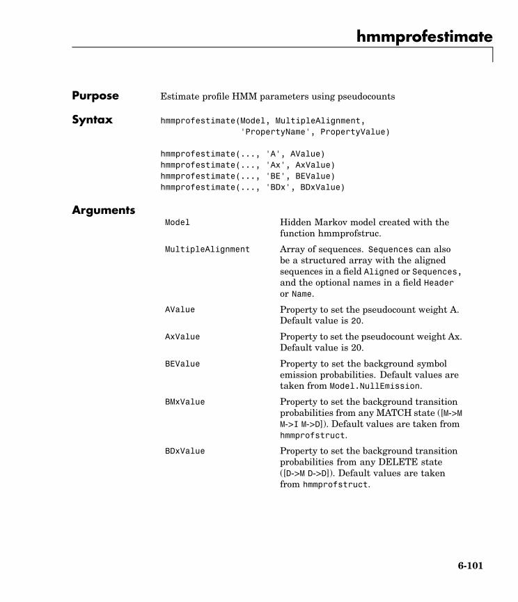
hmmprofestimate
Purpose Estimate profile HMM parameters using pseudocounts
Syntax hmmprofestimate(Model, MultipleAlignment,'PropertyName', PropertyValue)
hmmprofestimate(..., 'A', AValue)hmmprofestimate(..., 'Ax', AxValue)hmmprofestimate(..., 'BE', BEValue)hmmprofestimate(..., 'BDx', BDxValue)
ArgumentsModel Hidden Markov model created with the
function hmmprofstruc.
MultipleAlignment Array of sequences. Sequences can alsobe a structured array with the alignedsequences in a field Aligned or Sequences,and the optional names in a field Headeror Name.
AValue Property to set the pseudocount weight A.Default value is 20.
AxValue Property to set the pseudocount weight Ax.Default value is 20.
BEValue Property to set the background symbolemission probabilities. Default values aretaken from Model.NullEmission.
BMxValue Property to set the background transitionprobabilities from any MATCH state ([M->MM->I M->D]). Default values are taken fromhmmprofstruct.
BDxValue Property to set the background transitionprobabilities from any DELETE state([D->M D->D]). Default values are takenfrom hmmprofstruct.
6-101

hmmprofestimate
Description hmmprofestimate(Model, MultipleAlignment, 'PropertyName',PropertyValue) returns a structure with the fields containing theupdated estimated parameters of a profile HMM. Symbol emission andstate transition probabilities are estimated using the real counts andweighted pseudocounts obtained with the background probabilities.Default weight is A=20, the default background symbol emission formatch and insert states is taken from Model.NullEmission, and thedefault background transition probabilities are the same as defaulttransition probabilities returned by hmmprofstruct.
Model Construction: Multiple aligned sequences should containuppercase letters and dashes indicating the model MATCH andDELETE states agreeing with Model.ModelLength. If model stateannotation is missing, but MultipleAlignment is space aligned, then a"maximum entropy" criteria is used to select Model.ModelLength states.
Note: Insert and flank insert transition probabilities are not estimated,but can be modified afterwards using hmmprofstruct.
hmmprofestimate(..., 'A', AValue) sets the pseudocount weight A= Avalue when estimating the symbol emission probabilities. Defaultvalue is 20.
hmmprofestimate(...,'Ax', AxValue) sets the pseudocount weightAx = Axvalue when estimating the transition probabilities. Defaultvalue is 20.
hmmprofestimate(...,'BE', BEValue) sets the backgroundsymbol emission probabilities. Default values are taken fromModel.NullEmission.
hmmprofestimate(...,'BMx', BMxValue) sets the backgroundtransition probabilities from any MATCH state ([M->M M->I M->D]).Default values are taken from hmmprofstruct.
hmmprofestimate(..., 'BDx', BDxValue) sets the backgroundtransition probabilities from any DELETE state ([D->M D->D]). Defaultvalues are taken from hmmprofstruct.
6-102
hmmprofestimate
See Also Bioinformatics Toolbox functions hmmprofalign, hmmprofstruct,showhmmprof
6-103

hmmprofgenerate
Purpose Generate a random sequence drawn from the profile HMM
Syntax Sequence = hmmprofgenerate(Model,'PropertyName', PropertyValue)
[Sequence, Profptr] = hmmprofgenerage(Model)
hmmprofgenerate(..., 'Align', AlignValue)hmmprofgenerate(..., 'Flanks', FlanksValue)hmmprofgenerate(..., 'Signature', SignatureValue)
ArgumentsModel Hidden Markov model created with the
function hmmprofstruc.
AlignValue Property to control using upper caseletters for matches and lower case lettersfor inserted letters. Enter either true orfalse. The default value is false.
FlanksValue Property to control including the symbolsgenerated by the FLANKING INSERTstates in the output sequence. Enter eithertrue or false. The default values is false.
SignatureValue Property to control returning the mostlikely path and symbols. Enter either trueor false. Default value is false.
Description Seq = hmmprofgenerate(Model, 'PropertyName', PropertyValue)returns a string (Seq) showing a sequence of amino acids or nucleotidesdrawn from the profile (Model). The length, alphabet, and probabilitiesof the Model are stored in a structure. For move information aboutthis structure, see hmmprofstruct).
[Sequence, Profptr] = hmmprofgenerage(Model) returns a vector ofthe same length as the profile model pointing to the respective statesin the output sequence. Null pointers (0) mean that such states do notexist in the output sequence, either because they are never touched (i.e.
6-104

hmmprofgenerate
jumps from the BEGIN state to MATCH states or from MATCH statesto the END state), or because DELETE states are not in the outputsequence (not aligned output; see below).
hmmprofgenerate(..., 'Align', AlignValue) if Align is true, theoutput sequence is aligned to the model as follows: uppercase lettersand dashes correspond to MATCH and DELETE states respectively(the combined count is equal to the number of states in the model).Lowercase letters are emitted by the INSERT or FLANKING INSERTstates. If Align is false, the output is a sequence of uppercase symbols.The default value is true.
hmmprofgenerate(..., 'Flanks', FlanksValue) if Flanks is true,the output sequence includes the symbols generated by the FLANKINGINSERT states. The default value is false.
hmmprofgenerate(..., 'Signature', SignatureValue) if Signatureis true, returns the most likely path and symbols. The default valueis false.
Examples load('hmm_model_examples','model_7tm_2') % load a model examplerand_sequence = hmmprofgenerate(model_7tm_2)
See Also Bioinformatics Toolbox functions hmmprofalign, hmmprofstruct,showhmmprof
6-105

hmmprofmerge
Purpose Concatenate the prealigned strings of several sequences to a profileHMM
Syntax A = hmmprofmerge(Sequences)hmmprofmerge(Sequences, Names)hmmprofmerge(Sequences, Names, Scores)
ArgumentsSequences Array of sequences. Sequences can also
be a structured array with the alignedsequences in a field Aligned or Sequences,and the optional names in a field Headeror Name.
Names
Scores Pairwise alignment scores from thefunction hmmprofalign. Enter a vector ofvalues with the same length as the numberof sequences in Sequences.
Description hmmprofmerge(Sequences) displays a set of prealigned sequences to aHMM model profile. The output is aligned corresponding to the HMMstates.
• Match states — Uppercase letters
• Insert states — Lowercase letters or asterisks (*)
• Delete states — Dashes
Periods (.) are added at positions corresponding to inserts in othersequences. The input sequences must have the same number of profilestates, that is, the joint count of capital letters and dashes must bethe same.
hmmprofmerge(Sequences, Names) labels the sequences with Names.
6-106

hmmprofmerge
hmmprofmerge(Sequences, Names, Scores) sorts the displayedsequences using Scores.
Examples load('hmm_model_examples','model_7tm_2') %load modelload('hmm_model_examples','sequences') %load sequences
for ind =1:length(sequences)[scores(ind),sequences(ind).Aligned] =...
hmmprofalign(model_7tm_2,sequences(ind).Sequence);end
hmmprofmerge(sequences, scores)
See Also Bioinformatics Toolbox functions hmmprofalign, hmmprofstruct
6-107

hmmprofstruct
Purpose Create a profile HMM structure
Syntax Model = hmmprofstruct(Length)Model = hmmprofstruct(Length, 'Field1', FieldValues1,...)hmmprofstruct(Model, 'Field1', Field1Values1,...)
ArgumentsLength Number of match states in the model.
Model Hidden Markov model created with thefunction hmmprofstruc.
Field1 Field name in the structure Model. Entera name from the table below.
Description Model = hmmprofstruct(Length) returns a structure with the fieldscontaining the required parameters of a profile HMM. Length specifiesthe number of match states in the model. All other mandatory modelparameters are initialized to the default values.
Model = hmmprofstruct(Length, 'Field1', FieldValues1, ...)creates a profile HMM using the specified fields and parameters. Allother mandatory model parameters are initialized to default values.
hmmprofstruct(Model, 'Field1', Field1Values1, ...) returns theupdated profile HMM with the specified fields and parameters. All othermandatory model parameters are taken from the reference MODEL.
HMM Profile Structure Format
Model parameters fields (mandatory). All probability values are in the[0 1] range.
Field name Description
ModelLength Length of the profile (number of MATCH states)
Alphabet 'AA' or 'NT'. Default is 'AA’.
6-108

hmmprofstruct
MatchEmission Symbol emission probabilities in the MATCHstates
Size is [ModelLength x AlphaLength].
Note:
sum(S.MatchEmission,2) = [1;1;1; ... ;1]Default is 1/AlphaLength.
InsertEmission Symbol emission probabilities in the INSERTstate.
Size is [ModelLength x AlphaLength].
Note:
sum(S.InsertEmission,2) = [1;1;1; ... ;1]Default is 1/AlphaLength.
NullEmission Symbol emission probabilities in the MATCHand INSERT states for the NULL model. TheNULL model is used to compute the log-oddsratio at every state and avoid overflow when theprobabilities are propagated through the model.
Size is [1 x AlphaLength].
Note:
sum(S.NullEmission) = 1Default is 1/AlphaLength.
6-109

hmmprofstruct
BeginX BEGIN state transition probabilities
Format is
[B->D1 B->M1 B->M2 B->M3 .... B->Mend]
Notes:
sum(S.BeginX) = 1
For fragment profiles
sum(S.BeginX(3:end)) = 0
Default is [0.01 0.99 0 0 ... 0].
MatchX MATCH state transition probabilities
Format is
[M1->M2 M2->M3 ... M[end-1]->Mend;M1->I1 M2->I2 ... M[end-1]->I[end-1];M1->D2 M2->D3 ... M[end-1]->Dend;M1->E M2->E ... M[end-1]->E ]
Notes:
sum(S.MatchX) = [ 1 1 ... 1 ]
For fragment profiles
sum(S.MatchX(4,:)) = 0
Default is repmat([0.998 0.001 0.0010],profLength-1,1).
6-110

hmmprofstruct
InsertX INSERT state transition probabilities
Format is
[I1->M2 I2->M3 ... I[end-1]->Mend;[I1->I1 I2->I2 ... I[end-1]->I[end-1] ]
Note:
sum(S.InsertX) = [ 1 1 ... 1 ]
Default is repmat([0.5 0.5],profLength-1,1).
DeleteX DELETE state transition probabilities. Theformat is
[D1->M2 D2->M3 ... D[end-1]->Mend ;[D1->D2 D2->D3 ... D[end-1]->Dend ]
Note: sum(S.DeleteX) = [ 1 1 ... 1 ]
Default is repmat([0.5 0.5],profLength-1,1).
FlankingInsertX Flanking insert states (N and C) used for LOCALprofile alignment. The format is
[N->B C->T ;[N->N C->C ]
Note: sum(S.FlankingInsertsX) = [1 1]
To force global alignment use
S.FlankingInsertsX = [1 1; 0 0]
Default is [0.01 0.01; 0.99 0.99].
6-111

hmmprofstruct
LoopX Loop states transition probabilities used formultiple hits alignment. The format is
[E->C J->B ;E->J J->J ]
Note: sum(S.LoopX) = [1 1]
Default is [0.5 0.01; 0.5 0.99]
NullX Null transition probabilities used to providescores with log-odds values also for statetransitions. The format is
[G->F ; G->G]
Note: sum(S.NullX) = 1
Default is [0.01; 0.99]
Annotation fields (optional)
Name Model Name
IDNumber Identification Number
Description Short description of the model
A profile Markov model is a common statistical tool for modelingstructured sequences composed of symbols . These symbols includerandomness in both the output (emission of symbols) and the statetransitions of the process. Markov models are generally representedby state diagrams.
The figure shown below is a state diagram for a HMM profile of length 4.Insert, match, and delete states are in the regular part (middle section).
6-112

hmmprofstruct
• Match state means that the target sequence is aligned to the profileat the specific location,
• Delete state represents a gap or symbol absence in the targetsequence (also know as a silent state because it does not emit anysymbol),
• Insert state represents the excess of one or more symbols in thetarget sequence that are not included in the profile.
Flanking states (S, N, B, E, C, T) are used for proper modeling of theends of the sequence, either for global, local or fragment alignment ofthe profile. S, N, E, and T are silent while N and C are used to insertsymbols at the flanks.
Examples hmmprofstruct(100,'Alphabet','AA')
See Also Bioinformatics Toolbox functions gethmmprof, hmmprofalign,hmmprofestimate, hmmprofgenerate, hmmprofmerge, pfamhmmread,showhmmprof
6-113

imageneread
Purpose Read microarray data from an ImaGene Results file
Syntax GPRData = gprread('File','PropertyName', PropertyValue)
gprread(..., 'CleanColNames', CleanColNamesValue)
ArgumentsFile ImaGene Results formatted file Enter a
filename or a path and filename.
CleanColNameValue Property to control creating column namesthat MATLAB can use as variable names.
Description imagedata = imagegeenread(File, 'PropertyName',PropertyValue) reads ImaGene results data from File and creates aMATLAB structure imagedata containing the following fields:
HeaderAADataBlocksRowsColumnsFieldsIDsColumnNamesIndicesShape
imageneread(..., 'CleanColNames', CleanColNamesValue). AnImaGene file may contain column names with spaces and somecharacters that MATLAB cannot use in MATLAB variable names. IfCleanColNames is true, imagene returns ColumnNames that are validMATLAB variable names and names that you can use in functions.By default, CleanColNames is false and ColumnNames may containcharacters that are not valid for MATLAB variable names.
6-114

imageneread
The field Indices of the structure contains MATLAB indices that youcan use for plotting heat maps of the data with the functions imageor imagesc.
For more details on the ImaGene format and example data, see theImaGene User Manual. .
ImaGene is a registered trademark of BioDiscovery, Inc.
Examples % Read in a sample ImaGene file and plot the Signal Meancy3Data = imageneread('cy3.txt');maimage(cy3Data,'Signal Mean');
% Read in the Cy5 channel and create a loglog plot of Signal Mediancy5Data = imageneread('cy5.txt');sigMedianCol = find(strcmp('Signal Median',cy3Data.ColumnNames));cy3Median = cy3Data.Data(:,sigMedianCol);cy5Median = cy5Data.Data(:,sigMedianCol);maloglog(cy3Median,cy5Median,'title','Signal Median');
See Also The Bioinformatics Toolbox functions gprread, maboxplot, maimage,sptread
6-115

int2aa
Purpose Convert an amino acid sequence from an integer to a letterrepresentation
Syntax SeqChar = int2aa(SeqInt, 'PropertyName', PropertyValue)
int2aa(..., 'Case', CaseValue)
ArgumentsSeqInt Amino acid sequence represented with integers.
Enter a vector of integers from the table MappingAmino Acid Integers to Letters below. The arraydoes not have to be of type integer, but it doeshave to contain only integer numbers. Integers arearbitrarily assigned to IUB/IUPAC letters.
CaseValue Property to select the case of the returned characterstring. Enter either 'upper' or 'lower'. Defaultis 'upper'.
Mapping Amino Acid Integers to Letters
Amino Acid Code Amino Acid Code Amino Acid
Alanine A1 Isoleucine I10 Tyrosine Y19
Arginine R2 Leucine L11 Valine V20
Asparagine N3 Lysine K12 Asparticacid orAsparagine
B21
Aspartic acid(aspartate)
D4 Methionine M13 Glutamicacid orGlutamine
Z22
Cystine C5 Phenylalanine F14 Any aminoacid
X23
6-116

int2aa
Amino Acid Code Amino Acid Code Amino Acid
Glutamine Q6 Proline P15 Translationstop
*24
Glutamic acid(glutamate)
E7 Serine S16 Gap ofindeterminatelength
- 25
Glycine G8 Threonine T17 Unknown orany integernot in table
?0
Histidine H9 Tryptophan W18
Description SeqChar = int2aa(SeqInt, 'PropertyName', PropertyValue)converts a 1-by-N array of integers to a character string using the tableMapping Amino Acid Interger sot Letters above.
int2aa(..., 'Case', CaseValue) sets the output case of thenucleotide string. Default is uppercase.
Examples s = int2aa([13 1 17 11 1 21])
s =MATLAB
See Also Bioinformatics Toolbox functions aminolookup, aa2int, int2nt, nt2int
6-117

int2nt
Purpose Convert a nucleotide sequence from an integer to a letter representation
Syntax SeqChar = int2nt(SeqInt, 'PropertyName', PropertyValue)
int2nt(..., 'Alphabet', AlphabetValue)int2nt(..., 'Unknown', UnknownValue)int2nt(..., 'Case', CaseValue)
ArgumentsSeqInt Nucleotide sequence represented by integers.
Enter a vector of integers from the tableMapping Nucleotide Integers to Letters below.The array does not have to be of type integer,but it does have to contain only integernumbers. Integers are arbitrarily assigned toIUB/IUPAC letters.
AlphabetValue Property to select the nucleotide alphabet.Enter either 'DNA' or 'RNA'.
UnknownValue Property to select the integer value for theunknown character. Enter a character to mapintegers 16 or greater to an unknown character.The character must not be one of the nucleotidecharacters A, T, C, G or the ambiguous nucleotidecharacters N, R, Y, K, M, S, W, B, D, H, or V. Thedefault character is *.
CaseValue Property to select the letter case for thenucleotide sequence. Enter either 'upper' or'lower'. The default value is 'lower'.
6-118

int2nt
Mapping Nucleotide Integers to Letters
NucleotideBase
NucleotideBase
NucleotideBase
Adenosine 1–A R - A, G (purine) 6–R B - T, G, C 12–B
Cystine 2–C Y - T, C(pyrimidine)
7–Y D - A, T, G 13–D
Guanine 3–G K - G, T (keto) 8–K H - A, T, C 14–H
Thymidinewith Alphabet= 'DNA'
4–T M - A, C (amino) 9–M V - A, G, C 15–V
U - uridinewith Alphabet= 'RNA'
4–U S - G, C (strong) 10–S - Gap ofindeterminatelength
16–-
N - A, T, G, C
(any)
5–N W - A, T (weak) * Unknown(default)
0–*
Description int2nt(SeqNT, 'PropertyName', PropertyValue) converts a 1-by-Narray of integers to a character string using the table MappingNucleotide Letters to Integers above.
int2nt(..., 'Alphabet', AlphabetValue) defines the nucleotidealphabet to use. The default value is 'DNA', which uses the symbols A,T, C, and G. If Alphabet is set to 'RNA', the symbols A, C, U, G are usedinstead.
6-119

int2nt
int2nt(..., 'Unknown', UnknownValue) defines the character torepresent an unknown nucleotide base. The default character is '*'.
int2nt(..., 'Case', CaseValue) sets the output case of thenucleotide string. The default is uppercase.
Examples Enter a sequence of integers as a MATLAB vector (space orcomma-separated list with square brackets).
s = int2nt([1 2 4 3 2 4 1 3 2])
s =ACTGCTAGC
Define a symbol for unknown numbers 16 and greater.
si = [1 2 4 20 2 4 40 3 2];s = int2nt(si, 'unknown', '#')
s =ACT#CT#GC
See Also Bioinformatics Toolbox function aa2int, baselookup, int2aa, nt2int
6-120

isoelectric
Purpose Estimate the isoelectric point for an amino acid sequence
Syntax pI = isoelectric(SeqAA,)'PropertyName', PropertyValue
[pI Charge] = isoelectric(SeqAA,'PropertyName', PropertyValue)
isoelectric(..., 'PKVals', PKValsValue)isoelectric(..., 'Charge', ChargeValue)isoelectric(..., 'Chart', ChartValue)
ArgumentsSeqAA Amino acid sequence. Enter a character
string or a vector of integers from the table .Examples: 'ARN' or [1 2 3].
PKValsValue Property to provide alternative pK values.
ChargeValue Property to select a specific pH for estimatingcharge. Enter a number between 0 and 14. Thedefault value is 7.2.
ChartValue Property to control plotting a graph of chargeversus pH. Enter true or false.
Description isoelectric estimates the isoelectric point (the pH at which the proteinhas a net charge of zero) for an amino acid sequence and it estimatesthe charge for a given pH (default is pH 7.2). The estimates skewed bythe underlying assumptions that all amino acids are fully exposed tothe solvent, that neighboring peptides have no influence on the pK ofany given amino acid, and that the constitutive amino acids, as well asthe N- and C-termini, are unmodified. Cysteine residues participatingin disulfide bridges also affect the true pI and are not considered here.
6-121
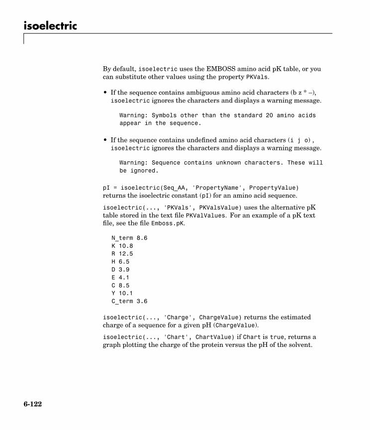
isoelectric
By default, isoelectric uses the EMBOSS amino acid pK table, or youcan substitute other values using the property PKVals.
• If the sequence contains ambiguous amino acid characters (b z * –),isoelectric ignores the characters and displays a warning message.
Warning: Symbols other than the standard 20 amino acidsappear in the sequence.
• If the sequence contains undefined amino acid characters (i j o) ,isoelectric ignores the characters and displays a warning message.
Warning: Sequence contains unknown characters. These willbe ignored.
pI = isoelectric(Seq_AA, 'PropertyName', PropertyValue)returns the isoelectric constant (pI) for an amino acid sequence.
isoelectric(..., 'PKVals', PKValsValue) uses the alternative pKtable stored in the text file PKValValues. For an example of a pK textfile, see the file Emboss.pK.
N_term 8.6K 10.8R 12.5H 6.5D 3.9E 4.1C 8.5Y 10.1C_term 3.6
isoelectric(..., 'Charge', ChargeValue) returns the estimatedcharge of a sequence for a given pH (ChargeValue).
isoelectric(..., 'Chart', ChartValue) if Chart is true, returns agraph plotting the charge of the protein versus the pH of the solvent.
6-122

isoelectric
Example % Get a sequence from PDB and estimate the isoelectric point.pdbSeq = getpdb('1CIV', 'SequenceOnly', true)% then estimate its isoelectric pointisoelectric(pdbSeq)
% plot the charge against the pH for a short polypeptide sequenceisoelectric('PQGGGGWGQPHGGGWGQPHGGGGWGQGGSHSQG', 'CHART', true)
% Get the Rh blood group D antigen from NCBI and calculates% its charge at pH 7.3 (typical blood pH)gpSeq = getgenpept('AAB39602')[pI Charge] = isoelectric(gpSeq, 'Charge', 7.38)
See Also Bioinformatics functions aacount, molweight
6-123
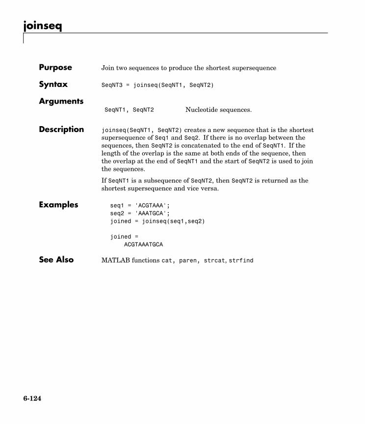
joinseq
Purpose Join two sequences to produce the shortest supersequence
Syntax SeqNT3 = joinseq(SeqNT1, SeqNT2)
ArgumentsSeqNT1, SeqNT2 Nucleotide sequences.
Description joinseq(SeqNT1, SeqNT2) creates a new sequence that is the shortestsupersequence of Seq1 and Seq2. If there is no overlap between thesequences, then SeqNT2 is concatenated to the end of SeqNT1. If thelength of the overlap is the same at both ends of the sequence, thenthe overlap at the end of SeqNT1 and the start of SeqNT2 is used to jointhe sequences.
If SeqNT1 is a subsequence of SeqNT2, then SeqNT2 is returned as theshortest supersequence and vice versa.
Examples seq1 = 'ACGTAAA';seq2 = 'AAATGCA';joined = joinseq(seq1,seq2)
joined =ACGTAAATGCA
See Also MATLAB functions cat, paren, strcat, strfind
6-124

maboxplot
Purpose Display a box plot for microarray data
Syntax maboxplot(Data, 'PropertyName', PropertyValue)maboxplot(Data, ColumnName)maboxplot(MasStruct, FieldName)
maboxplot(..., 'Title', TitleValue)maboxplot(..., 'Notch', NotchValue)maboxplot(..., 'Symbol', SymbolValue)maboxplot(..., 'Orientation', OrientationValue)maboxplot(..., 'WhiskerLength', WhiskerLengthValue)
H = maboxplot(...)[H, HLines] = maboxplot(...)
Description maboxplot(Data, 'PropertyName', PropertyValue) displays a boxplot of the values in the columns of Data. Data can be a numeric arrayor a structure containing a field called Data.
maboxplot(Data,ColumnName) labels the box plot column names. Formicroarray data structures that are block based, maboxplot creates abox plot of a given field for each block.
maboxplot(MasStruct, FieldName) displays a box plot of fieldFieldName for each block in microarray data structure MasStruct.
maboxplot(..., 'Title', TitleValue) allows you to specify the titleof the plot. The default Title is FieldName.
maboxplot(..., 'Notch', NotchValue) if Notch is true, drawsnotched boxes. The default is false to show square boxes.
maboxplot(..., 'Symbol', SymbolValue) allows you to specify thesymbol used for outlier values. The default Symbol is '+'.
maboxplot(..., 'Orientation', OrientationValue) allows you tospecify the orientation of the box plot. The choices are 'Vertical’ and'Horizontal'. The default is 'Vertical'.
6-125

maboxplot
maboxplot(..., 'WhiskerLength', WhiskerLengthValue) allows youto specify the whisker length for the box plot. WhiskerLength definesthe maximum length of the whiskers as a function of the interquartilerange (IQR) (default = 1.5). The whisker extends to the most extremedata value within WhiskerLength*IQR of the box. If WhiskerLength =0, then maboxplot displays all data values outside the box, using theplotting symbol Symbol.
H = maboxplot(...) returns the handle of the box plot axes.
[H, HLines] = maboxplot(...) returns the handles of the lines usedto separate the different blocks in the image.
Examples load yeastdatamaboxplot(yeastvalues,times);xlabel('Sample Times');
% Using a structuregeoStruct = getgeodata('GSM1768');maboxplot(geoStruct);
% For block-based datamadata = gprread('mouse_a1wt.gpr');maboxplot(madata,'F635 Median');figuremaboxplot(madata,'F635 Median - B635','TITLE',...
'Cy5 Channel FG - BG');
See Also Bioinformatics Toolbox functions maboxplot, maimage, mairplot,maloglog, malowess
Statistics Toolbox function boxplot
6-126

maimage
Purpose Display a spatial image for microarray data
Syntax maimage(X, FieldName, 'PropertyName', PropertyValue)
maimage(..., 'Title', TitleValue)maimage(..., 'ColorBar', ColorBarValue)maimage(..., 'HandleGraphicsPropertyName' PropertyValue)H = maimage(...)[H, HLines] = maimage(...)
Description maimage(X, FieldName, 'PropertyName', PropertyValue) displaysan image of field FieldName from microarray data structure X.Microarray data can be GenPix Results (GPR) format.
maimage(..., 'Title', TitleValue) allows you to specify the title ofthe plot. The default title is FieldName.
maimage(..., 'ColorBar', ColorBarValue) if ColorBar is true, acolorbar is shown. If ColorBar is false, no colorbar is shown. Thedefault is for the colorbar to be shown.
maimage(..., 'HandleGraphicsPropertyName' PropertyValue)allows you to pass optional Handle Graphics property name/propertyvalue pairs to the function. For example, a name/value pair for colorcould be maimage(..., 'color' 'r').
H = maimage(...) returns the handle of the image.
[H, HLines] = maimage(...) returns the handles of the lines used toseparate the different blocks in the image.
Examples madata = gprread('mouse_a1wt.gpr');maimage(madata,'F635 Median');
maimage(madata,'F635 Median - B635',...'Title','Cy5 Channel FG - BG');
See Also Bioinformatics Toolbox functions mairplot, maloglog
6-127

mairplot
Purpose Display intensity versus ratio scatter plot for microarray signals
Syntax mairplot(X, Y, 'PropertyName', PropertyValue)
mairplot(..., 'FactorLines', FactorLinesValue)mairplot(..., 'Title', TitleValue)mairplot(..., 'Labels', LabelsValue)mairmage(..., 'HandleGraphicsPropertyName' PropertyValue)[Intensity, Ratio] = mairplot(...)[Intensity, Ratio, H] = mairplot(...)
ArgumentsX, Y
FactorLinesValue Property to specify a factor of change.
TitleValue Property to specify a title for the plot.
LabelsValue Property to specify labels for the plot.
HandleGraphicsValue Property to pass optional propertyname/value pairs from Handle Graphics.
Description mairplot(X, Y, 'PropertyName', PropertyValue) creates anintensity versus ratio scatter plot of X versus Y.
mairplot(..., 'FactorLines', FactorLinesValue) adds linesshowing a factor of N change.
mairplot(..., 'Title', TitleValue) allows you to specify a titlefor the plot.
mairplot(..., 'Labels', LabelsValue) allows you to specify a cellarray of labels for the data. If labels are defined, then clicking a pointon the plot shows the label corresponding to that point.
maimage(..., 'HandleGraphicsPropertyName' PropertyValue)allows you to pass optional Handle Graphics property name/propertyvalue pairs to the function.
6-128

mairplot
[Intensity, Ratio] = mairplot(...) returns the intensity and ratiovalues.
[Intensity, Ratio, H] = mairplot(...) returns the handle of theplot.
Examples maStruct = gprread('mouse_a1wt.gpr');cy3data = maStruct.Data(:,36);cy5data = maStruct.Data(:,37);positiveVals = (cy3data>0) & (cy5data>0);cy3data(~positiveVals) = [];cy5data(~positiveVals) = [];mairplot(cy3data,cy5data,'title','R vs G')figurenames = maStruct.Names(positiveVals);mairplot(cy3data,cy5data,'FactorLines',2,...
'Labels',maStruct.Names)
See Also Bioinformatics Toolbox functions maboxplot, maloglog, malowess
6-129

maloglog
Purpose Create a loglog plot of microarray data
Syntax maloglog(X, Y, 'PropertyName', PropertyValue)
maloglog(..., 'FactorLines', FactorLinesValue)maloglog(..., 'Title', TitleValue)maloglog(..., 'Labels', LablesValues)maloglog(..., HandleGraphics name/value)H = maloglog(...)
Description maloglog(X, Y, 'PropertyName', PropertyValue) creates a loglogscatter plot of X versus Y.
maloglog(..., 'FactorLines', N) adds lines showing a factor of Nchange.
maloglog(..., 'Title', TitleValue) allows you to specify a titlefor the plot.
maloglog(..., 'Labels', LabelsValues) allows you to specify a cellarray of labels for the data. If Labels is defined, then clicking a point onthe plot shows the label corresponding to that point.
maloglog(..., HandleGraphics name/value) allows you to passoptional Handle Graphics property name/property value pairs to thefunction.
H = maloglog(...) returns the handle to the plot.
Examples maStruct = gprread('mouse_a1wt.gpr');Red = maStruct.Data(:,4);Green = maStruct.Data(:,13);maloglog(Red, Green, 'title', 'Red versus Green')figuremaloglog(Red, Green, 'FactorLines', 2,...
'Labels', maStruct.Names)
See Also Bioinformatics Toolbox functions maboxplot, mairplot
6-130

malowess
Purpose Smooth microarray data using the Lowess method
Syntax YSmooth = malowess(X, Y, 'PropertyName', PropertyValue)
malowess(..., 'Order', OrderValue)malowess(..., 'Robust', RobustValue)malowess(..., 'Span', SpanValue)
ArgumentsX, Y Scatter data.
OrderValue Property to select the order of the algorithm.Enter either 1 (linear fit) or 2 (quadratic fit).The default order is 1.
RubustValue Property to select a robust fit. Enter eithertrue or false.
SpanValue Property to specify the window size. Thedefault value is 0.05 (5% of total points in X)
Description YSmooth = malowess(X, Y, 'PropertyName', PropertyValue)smooths scatter data (X, Y) using the Lowess smoothing method. Thedefault window size is 5% of the length of X.
malowess(..., 'Order', OrderValue) chooses the order of thealgorithm. Note that the MATLAB Curve Fitting Toolbox refers toLowess smoothing of order 2 as Loess smoothing.
malowess(..., 'Robust', RobustValue) uses a robust fit whenRobust is set to true. This option can take a long time to calculate.
malowess(..., 'Span', SpanValue) modifies the window size for thesmoothing function. If Span is less than 1, the window size is taken tobe a fraction of the number of points in the data. If Span is greaterthan 1, the window is of size Span.
Examples maStruct = gprread('mouse_a1wt.gpr');cy3data = maStruct.Data(:,4);
6-131

malowess
cy5data = maStruct.Data(:,13);[x,y] = mairplot(cy3data, cy5data);drawnowysmooth = malowess(x,y);hold on;plot(x,ysmooth,'rx');ynorm = y - ysmooth;
See Also Bioinformatics Toolbox functions mairplot, maloglog, mamadnorm,mameannorm
6-132

mamadnorm
Purpose Normalize microarray data by median absolute deviation (MAD)
Syntax XNorm = mamadnorm(X, 'PropertyName', PropertyValue)[XNorm, MAD] = mamadnorm(X)
mamadnorm(..., 'Global', GlobalValue)
Description XNorm = mamadnorm(X, 'PropertyName', PropertyValue) divides thevalues in each column of X by the MAD of the column.
[XNorm, MAD] = mamadnorm(X) returns the median absolute deviation.
mamadnorm(..., 'Global', GlobalValue) if Global is true, dividesthe values in the data set by the global MAD, as opposed to the MAD ofeach column of the data.
Examples maStruct = gprread('mouse_a1wt.gpr');Red = maStruct.Data(:,4);Green = maStruct.Data(:,13);maloglog(Red,Green,'factorlines',true)figurenormRed = mamadnorm(Red);normGreen = mamadnorm(Green);maloglog(normRed,normGreen,'title','Normalized',...
'factorlines',true)
See Also Bioinformatics Toolbox functions malowess, mameannorm
6-133

mameannorm
Purpose Normalize microarray data using the global mean
Syntax XNorm = mameannorm(X, 'PropertyName', PropertyValue)[XNorm, ColMean] = mameannorm(X)
mameannorm(..., 'Prctile', PrctileValue)mameannorm(..., 'Global', GlobalValue)
Description XNorm = mameannorm(X, 'PropertyName', PropertyValue) dividesthe values in each column of X by the mean column intensity.
[XNorm, ColMean] = mameannorm(X) returns the column means usedto scale the data.
mameannorm(..., 'Prctile', PrctileValue) scales the mean of thepercentile Prctile for the data. This is useful to prevent large outliersfrom skewing the normalization.
mameannorm(..., 'Global', GlobalValue) if Global is true, dividesthe values in the data set by the global mean of the data, as opposed tothe mean of each column of the data.
Examples maStruct = gprread('mouse_a1wt.gpr');Red = maStruct.Data(:,4);Green = maStruct.Data(:,13);maloglog(Red,Green,'factorlines',true)figurenormRed = mameannorm(Red);normGreen = mameannorm(Green);maloglog(normRed,normGreen,'title','Normalized',...
'factorlines',true)
See Also Bioinformatics Toolbox functions malowess, mamadnorm
6-134

mapcaplot
Purpose Creates a Principal Component plot of expression profile data
Syntax mapcaplot(Data)mapcaplot(Data,Label)
ArgumentsData Microarray data
Label Data point labels.
Description mapcaplot(Data) creates 2D scatter plots of principal components ofthe array DATA. The principal components used for the x and y data areselected from popup menus, below each scatter plot.
Once the principal components have been plotted, a region can beselected in either axes with the mouse. This will highlight the pointsin the selected region, and the corresponding points in the other axes.This will also display a list of the row numbers of the selected pointsin the list box. Selecting an entry in the list box will display a labelwith the row number in each axes, at the corresponding point. Clickingon a point in the scatter plot will display a label with its row numberuntil the mouse is released.
mapcaplot(Data,Label) uses the elements of the cell array of stringsLabel, instead of the row numbers, to label the data points.
Examples load filteredyeastdatamapcaplot(yeastvalues,genes)
See Also Bioinformatics Toolbox function clustergram
Statistical Toolbox function princomp
6-135

molweight
Purpose Calculate the molecular weight of an amino acid sequence
Syntax molweight(SeqAA)
ArgumentsSeqAA Amino acid sequence. Enter a character string or a
vector of integers from the table . Examples: 'ARN',[1 2 3]. You can also enter a structurewith the field Sequence.
Description molweight(SeqAA) calculates the molecular weight for the amino acidsequence SeqAA.
Examples Get the protein sequence for cytochrome c and determine its molecularweight.
pirdata = getpir('cchu','SequenceOnly',true)mwcchu = molweight(pirdata)
mwcchu =1.1749e+004
See Also Bioinformatics Toolbox functions aacount, atomiccomp
6-136
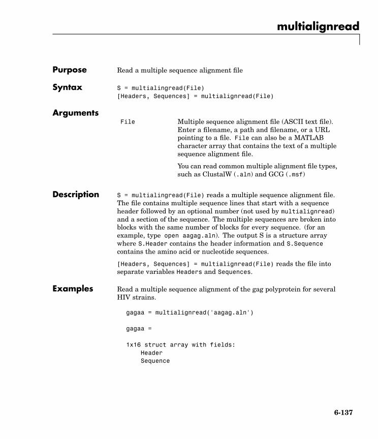
multialignread
Purpose Read a multiple sequence alignment file
Syntax S = multialingread(File)[Headers, Sequences] = multialignread(File)
ArgumentsFile Multiple sequence alignment file (ASCII text file).
Enter a filename, a path and filename, or a URLpointing to a file. File can also be a MATLABcharacter array that contains the text of a multiplesequence alignment file.
You can read common multiple alignment file types,such as ClustalW (.aln) and GCG (.msf)
Description S = multialingread(File) reads a multiple sequence alignment file.The file contains multiple sequence lines that start with a sequenceheader followed by an optional number (not used by multialignread)and a section of the sequence. The multiple sequences are broken intoblocks with the same number of blocks for every sequence. (for anexample, type open aagag.aln). The output S is a structure arraywhere S.Header contains the header information and S.Sequencecontains the amino acid or nucleotide sequences.
[Headers, Sequences] = multialignread(File) reads the file intoseparate variables Headers and Sequences.
Examples Read a multiple sequence alignment of the gag polyprotein for severalHIV strains.
gagaa = multialignread('aagag.aln')
gagaa =
1x16 struct array with fields:HeaderSequence
6-137

multialignread
Create a phylogenetic tree with multiply aligned sequences.
Sequences = multialignread('aagag.aln')distances = seqpdist(Sequences)tree = seqlinkage(distances)phytreetool(tree)
See Also Bioinformatics Toolbox function fastaread, gethmmalignment
6-138

nmercount
Purpose Count the number of n-mers in a nucleotide or amino acid sequence
Syntax nmercount(Seq, Length)
ArgumentsSeq Nucleotide or amino acid sequence. Enter a
character string or a structure with the fieldSequence.
Length Length of n-mer to count. Enter an integer.
Description nmercount(Seq, Length) counts the number of n-mers or patternsof a specific length in a sequence.
Examples Count the number of n-mers in an amino acid sequence and displaythe first six rows in the cell array.
S = getgenpept('AAA59174','SequenceOnly',true)nmers = nmercount(S,4);nmers(1:6,:)
ans ='apes' [2]'dfrd' [2]'eslk' [2]'frdl' [2]'gnys' [2]'lkel' [2]
See Also Bioinformatics Toolbox functions basecount, codoncount, dimercount
6-139

nt2aa
Purpose Convert a sequence of nucleotides to a sequence of amino acids
Syntax SeqAA = nt2aa(SeqNT, 'PropertyName', PropertyValue)
nt2aa(..., 'Frame', FrameValue)nt2aa(..., 'GeneticCode', GeneticCodeValue)nt2aa(..., 'AlternativeStartCodons', AlternativeValue)
ArgumentsSeqNT DNA nucleotide sequence. Enter a character
string with only the characters A, T, C, and G.You cannot use the character U, ambiguouscharacters, or a hyphen. You can also enter astructure with the field Sequence.
FrameValue Property to select a frame. Enter 1, 2, 3, or'ALL'. The default value is 1.
GeneticCodeValue Property to select a genetic code. Enter a codenumber or code name from the table GeneticCode on page 6-140. If you use a code name,you can truncate the name to the first twocharacters of the name.
AlternativeValue Property to control the use of alternativecodons. Enter either true or false. Thedefault value is true.
Genetic Code
Code Number Code Name
1 Standard
2 Vertebrate Mitochondrial
3 Yeast Mitochondrial
6-140

nt2aa
Code Number Code Name
4 Mold, Protozoan, andCoelenterate Mitochondrial andMycoplasma/Spiroplasma
5 Invertebrate Mitochondrial
6 Ciliate, Dasycladacean, and HexamitaNuclear
9 Echinoderm Mitochondrial
10 Euplotid Nuclear
11 Bacterial and Plant Plastid
12 Alternative Yeast Nuclear
13 Ascidian Mitochondrial
14 Flatworm Mitochondrial
15 Blepharisma Nuclear
16 Chlorophycean Mitochondrial
21 Trematode Mitochondrial
22 Scenedesmus Obliquus Mitochondrial
23 Thraustochytrium Mitochondrial
Description SeqAA = nt2aa(SeqNT, 'PropertyName', PropertyValue) convertsa nucleotide sequence to an amino acid sequence using the standardgenetic code.
nt2aa(..., 'Frame', FrameValue) converts a nucleotide sequencefor a specific reading frame to an amino acid sequence. If FrameValueequals 'ALL', then the three reading frames are converted and theoutput is a 3-by-1 cell array.
nt2aa(..., 'GeneticCode', GeneticCodeValue) converts a nucleotidesequence to an amino acid sequence using a specific genetic code.
6-141

nt2aa
nt2aa(..., 'AlternativeStartCodons', AlternativeValue) controlsthe use of alternative start codons. By default, AlternativeStartCodonsis set to true, and if the first codon of a sequence corresponds to aknown alternative start codon, the codon is translated to methionine.
If this option is set to false, then alternative start codons at the startof a sequence are translated to their corresponding amino acids for thegenetic code that you use, which might not necessarily be methionine.For example, in the human mitochondrial genetic code, AUA and AUU areknown to be alternative start codons.
For more details of alternative start codons, see
www.ncbi.nlm.nih.gov/Taxonomy/Utils/wprintgc.cgi?mode=t#SG1
Examples Convert the gene ND1 on the human mitochondria genome.
mitochondria = getgenbank('NC_001807','SequenceOnly',true)gene = mitochondria (3308;4264)protein1 = nt2aa(gene,'GeneticCode', 2)protein2 = getgenpept('NP_536843',SequenceOnly',true)
Convert the gene ND2 on the human mitochondria genome. In thiscase, the first codon is att, which is converted to M, while the followingatt codons are converted to I. If you set 'AlternativeStartCodons' tofalse, then the first codon att is converted to I.
mitochondria = getgenbank('NC_001807','SequenceOnly',true)gene = mitochondria (3371:4264)protein1 = nt2aa(gene,'GeneticCcode',2)protein2 = getgenpept('NP_536844', 'SequenceOnly',true)
See Also Bioinformatics Toolbox functions aa2nt, baselookup, geneticcode,revgeneticcode
6-142

nt2int
Purpose Convert a nucleotide sequence from a letter to an integer representation
Syntax SeqInt = nt2int(SeqChar, 'PropertyName', PropertyValue)
nt2int(..., 'Unknown', UnknownValue)nt2int(..., 'ACGTOnly', ACGTOnlyValue)
ArgumentsSeqNT Nucleotide sequence represented with letters.
Enter a character string from the table MappingNucleotide Letters to Integers below. Integersare arbitrarily assigned to IUB/IUPAC letters. Ifthe property ACGTOnly is true, you can only enterthe characters A, C, T, G, and U.
UnknownValue Property to select the integer for unknowncharacters. Enter an integer. Maximum value is255. Default value is 0.
ACGTOnlyValue Property to control the use of ambiguousnucleotides. Enter either true or false. Defaultvalue is false.
Mapping Nucleotide Letters to Integers
Base Code Base Code Base Code
Adenosine A—1 A, G (purine) R—6 T, G, C R—12
Cytidine C—2 T, C(pyrimidine)
Y—7 A, T, G Y—13
Guanine G—3 G, T (keto) K—8 A, T, C K—14
Thymidine T—4 A, C (amino) M—9 A, G, C V—15
6-143

nt2int
Base Code Base Code Base Code
Uridine U—4 G, C (strong) S—10 Gap ofindeterminatelength
-—16
A, T, G, C (any) N—5 A, T (weak) W—11 Unknown(default)
*—0
Description nt2int(SeqNT, 'PropertyName', PropertyValue) converts acharacter string of nucleotides to a 1-by-N array of integers usingthe table Mapping Nucleotide Letters to Integers above. Unknowncharacters (characters not in the table) are mapped to 0. Gapsrepresented with hyphens are mapped to 16.
nt2int(SeqNT,'Unknown',UnknownValue) defines the number used torepresent unknown nucleotides. The default value is 0.
nt2int(SeqNT,'ACGTOnly', ACGTONlyValue) if ACGTOnly is true, theambiguous nucleotide characters (N, R, Y, K, M, S, W, B, D, H, and V) arerepresented by the unknown nucleotide number.
Examples Convert a nucleotide sequence with letters to integers.
s = nt2int('ACTGCTAGC')
s =1 2 4 3 2 4 1 3 2
See Also Bioinformatics Toolbox function aa2int, baselookup, int2aa, int2nt
6-144

ntdensity
Purpose Plot the density of nucleotides along a sequence
Syntax ntdensity(SeqNT, 'PropertyName', PropertyValue)
ntdenstiy(..., 'Window', WindowValue)[Density, HighCG] = ntdensity(..., 'CGThreshold',CGThresholdValue)
Description ntdensity(SeqNT) plots the density of nucleotides A, T, C, G in sequenceSeqNT.
Denstity = ntdensity(SeqNT, 'PropertyName', PropertyValue)returns a MATLAB structure with the density of nucleotides A, C, G,and T.
ntdensity(..., 'Window', WindowValue) uses a window oflength Window for the density calculation. The default value islength(SeqNT)/20.
[Density, HighCG] = ntdensity(..., 'CGThreshold',CGThresholdValue) returns indices for regions where the CG content ofSeqNT is greater than CGThreshold. The default value for CGThresholdis 5.
Examples s = randseq(1000, 'alphabet', 'dna');ndensity(s)
6-145

ntdensity
See Also Bioinformatics Toolbox functions basecount, codoncount, dimercount
MATLAB function filter
6-146

nuc44
Purpose Return a NUC44 scoring matrix for nucleotide sequences
Syntax ScoringMatrix = nuc44
Description The nuc44 scoring matrix uses ambiguous nucleotide codes andprobabilities rounded to the nearest integer.
Scale = 0.277316
Expected score = -1.7495024, Entropy = 0.5164710 bits
Lowest score = -4, Highest score = 5
Order: A C G T R Y K M S W B D H V N
[Matrix, MatrixInfo] = nuc44 returns the structure of informationabout the matrix with Name and Order.
6-147
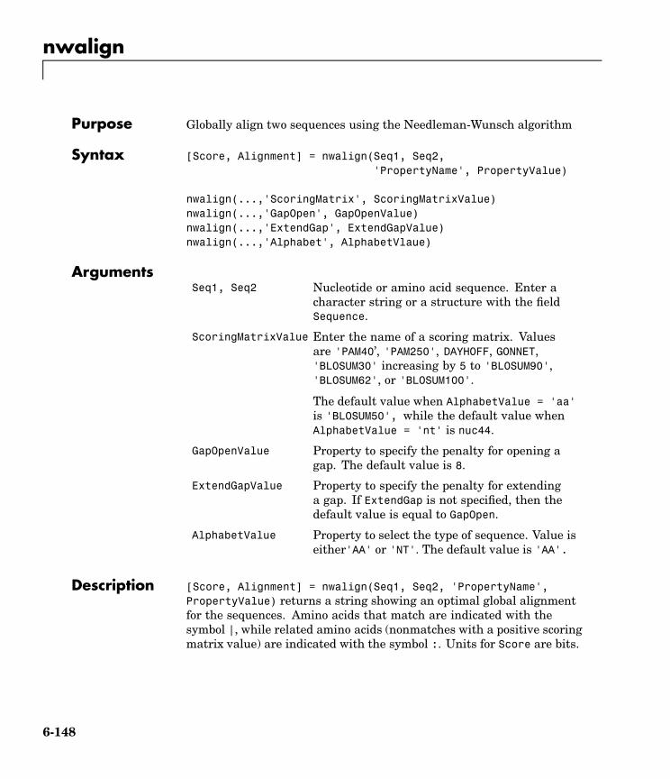
nwalign
Purpose Globally align two sequences using the Needleman-Wunsch algorithm
Syntax [Score, Alignment] = nwalign(Seq1, Seq2,'PropertyName', PropertyValue)
nwalign(...,'ScoringMatrix', ScoringMatrixValue)nwalign(...,'GapOpen', GapOpenValue)nwalign(...,'ExtendGap', ExtendGapValue)nwalign(...,'Alphabet', AlphabetVlaue)
ArgumentsSeq1, Seq2 Nucleotide or amino acid sequence. Enter a
character string or a structure with the fieldSequence.
ScoringMatrixValue Enter the name of a scoring matrix. Valuesare 'PAM40’, 'PAM250', DAYHOFF, GONNET,'BLOSUM30' increasing by 5 to 'BLOSUM90','BLOSUM62', or 'BLOSUM100'.
The default value when AlphabetValue = 'aa'is 'BLOSUM50', while the default value whenAlphabetValue = 'nt' is nuc44.
GapOpenValue Property to specify the penalty for opening agap. The default value is 8.
ExtendGapValue Property to specify the penalty for extendinga gap. If ExtendGap is not specified, then thedefault value is equal to GapOpen.
AlphabetValue Property to select the type of sequence. Value iseither'AA' or 'NT'. The default value is 'AA'.
Description [Score, Alignment] = nwalign(Seq1, Seq2, 'PropertyName',PropertyValue) returns a string showing an optimal global alignmentfor the sequences. Amino acids that match are indicated with thesymbol |, while related amino acids (nonmatches with a positive scoringmatrix value) are indicated with the symbol :. Units for Score are bits.
6-148

nwalign
nwalign(..., 'ScoringMatrix', ScoringMatirxValue) specifies thescoring matrix to use for the alignment.
nwalign(..., 'GapOpen', GapOpenValue) specifies the penalty foropening a gap in the alignment.
nwalign(..., 'ExtendGap', ExtendGapValue) specifies the penaltyfor extending a gap in the alignment. If ExtendGap is not specified, thenextensions to gaps are scored with the same value as GapOpen.
nwalign(..., 'Alphabet', AlphabetValue) specifies amino acid ornucleotide sequences.
Examples Globally align two amino acid sequences.
[Score, Alignment] = nwalign('VSPAGMASGYD','IPGKASYD')
Score =7.3333
Alignment =VSPAGMASGYD: | | || ||I-P-GKAS-YD
Select scoring matrix and gap penalty.
[Score, Alignment] = nwalign('IGRHRYHIGG','SRYIGRG',...'scoringmatrix','pam250',...'gapopen',5)
Score =2.3333
Alignment =
IGRHRYHIG-G: || || |
-S--RY-IGRG
6-149

nwalign
See Also Bioinformatics Toolbox functions blosum, dayhoff, gonnet, nt2aa,showalignment, swalign
6-150

palindromes
Purpose Find palindromes in a sequence
Syntax [Position, Length] = palindromes(SeqNT,'PropertyName',
PropertyValue)[Postion, Length, Pal] = palindromes(SeqNT)
palindromes(..., 'Length', LengthValue)palindromes(..., 'Complement', ComplementValue)
Description [Position, Length] = palindromes(SeqNT, 'PropertyName',PropertyValue) finds all palindromes in sequence SeqNT with a lengthgreater than or equal to 6, and returns the starting indices, Position,and the lengths of the palindromes, Length.
[Position, Length, Pal] = palindromes(SeqNT) also returns a cellarray Pal of the palindromes.
palindromes(..., 'Length',LengthValue) finds all palindromeslonger than or equal to Length. The default value is 6.
palindromes(..., 'Complement', ComplementValue) findscomplementary palindromes if Complement is true, that is, where theelements match their complementary pairs A-T(or U) and C-G instead ofan exact nucleotide match.
Examples [p,l,s] = palindromes('GCTAGTAACGTATATATAAT')
p =1112
l =77
s ='TATATAT''ATATATA'
6-151

palindromes
[pc,lc,sc] = palindromes('GCTAGTAACGTATATATAAT',...'Complement',true);
Find the palindromes in a random nucleotide sequence.
a = randseq(100)
a =TAGCTTCATCGTTGACTTCTACTAAAAGCAAGCTCCTGAGTAGCTGGCCAAGCGAGCTTGCTTGTGCCCGGCTGCGGCGGTTGTATCCTGAATACGCCAT
[pos,len,pal]=palindromes(a)
pos =74
len =6
pal ='GCGGCG'
See Also Bioinformatics Toolbox functions seqrcomplement, seqshowwords
MATLAB functions regexp, strfind
6-152

pam
Purpose Return a PAM scoring matrix
Syntax ScoringMatrix = pam(N, 'PropertyName', PropertyValue)[ScoringMatirx, MatrixInfo] = pam(N)
ScoringMatrix = pam(..., 'Extended', ExtendedValue)ScoringMatrix = pam(..., 'Order', 'OrderString')
ArgumentsN Enter values 10:10:500. The default ordering
of the output is A R N D C Q E G H I L K MF P S T W Y V B Z X *.
Entering a larger value for N to allow sequencealignments with larger evolutionary distances.
ExtendedValue Property to add ambiguous characters to thescoring matrix. Enter either true or false.Default is false.
OrderString Property to control the order of amino acids inthe scoring matrix. Enter a string with at leastthe 20 standard amino acids.
Description ScoringMatrix = pam(N, 'PropertyName', PropertyValue) returnsa PAM scoring matrix for amino acid sequences.
[ScoringMatrix, MatrixInfo] = pam(N) returns a structure withinformation about the PAM matrix. The fields in the structure are Name,Scale, Entropy, Expected, and Order.
B = pam(..., 'Extended', 'ExtendedValue') if Extended is true,returns a scoring matrix with the 20 amino acid characters, theambiguous characters, and stop character (B, Z, X, *), . If Extended isfalse, only the standard 20 amino acids are included in the matrix.
B = pam(..., 'Order', 'OrderString') returns a PAM matrixordered by the amino acid sequence in Order. If Order does not contain
6-153

pam
the extended characters B, Z, X, and *, then these characters are notreturned.
PAM50 substitution matrix in 1/2 bit units, Expected score = -3.70,Entropy = 2.00 bits, Lowest score = -13, Highest score = 13.
PAM250 substitution matrix in 1/3 bit units, Expected score = -0.844,Entropy = 0.354 bits, Lowest score = -8, Highest score = 17.
Examples Get the PAM matrix with N = 50.
PAM50 = pam(50)
PAM250 = pam(250,'Order','CSTPAGNDEQHRKMILVFYW')
See Also Bioinformatics Toolbox functions blosum, dayhoff, gonnet, nwalign,swalign
6-154
pdbdistplot
Purpose Visualize the intermolecular distances in a PDB file
Syntax pdbdistplot('PDBid')pdbdistplot('PDBid', Distance)
ArgumentsPDBid Unique identifier for a protein structure record. Each
structure in the PDB is represented by a 4-characteralphanumeric identifier.
For example, 4hhb is the identification code forhemoglobin.
Distance Threshold distance in Angstroms shown on a spy plot.Default value is 7.
Description pdbdistplot displays the distances between atoms and amino acidsin a PDB structure.
pdbdistplot('PDBid') retrieves the entry PDBid from the ProteinData Bank (PDB) database and creates a heat map showing interatomdistances and a spy plot showing the residues where the minimumdistances apart are less than 7 Angstroms. PDBid can also be the nameof a variable or a file containing a PDB MATLAB structure.
pdbdistplot('PDBid', Distance) specifies the threshold distanceshown on a spy plot.
Examples Show spy plot at 7 Angstroms of the protein cytochrome C from albacoretuna.
pdbdistplot('5CYT');
Now take a look at 10 Angstroms.
pdbdistplot('5CYT',10);
See Also Bioinformatics Toolbox functions getpdb, pdbread
6-155

pdbread
Purpose Read data from a Protein Data Bank (PDB) file
Syntax PDBData = pdbread('File')
ArgumentsFile Protein Data Bank (PDB) formatted file (ASCII text file).
Enter a filename, a path and filename, or a URL pointingto a file. File can also be a MATLAB character array thatcontains the text for a PDB file.
Description The Protein Data Bank (PDB) is an archive of experimentallydetermined three-dimensional protein structures. pdbread reads datafrom a PDB formatted file into MATLAB.
PDBData = pdbread('File') reads the data in PDB formatted text fileFile and stores the data in the MATLAB structure PDBData.
The data stored in each record of the PDB file is converted, whereappropriate, to a MATLAB structure. For example, the ATOM recordsin a PDB file are converted to an array of structures with the followingfields: AtomSerNo, AtomName, altLoc, resName, chainID, resSeq, iCode,X, Y, Z, occupancy, tempFactor, segID, element, and charge.
The sequence information from the PDB file is stored in the Sequencefield of PDBData. The sequence information is itself a structure with thefields NumOfResidues, ChainID, ResidueNames, and Sequence. The fieldResidueNames contains the three-letter codes for the sequence residues.The field Sequence contains the single-letter codes for the sequence. Ifthe sequence has modified residues, then the ResidueNames might notcorrespond to the standard three-letter amino acid codes, in which casethe field Sequence will contain a ? in the position corresponding tothe modified residue.
For more information about the PDB format, see
http://www.rcsb.org/pdb/docs/format/pdbguide2.2/guide2.2_frame.html
6-156

pdbread
Examples Get information for the human hemoglobin protein with number 1A00from the Protein Data Bank, store information in the file collagen.pdb,and then read the file back into MATLAB.
getpdb( '1A00','ToFile', 'collagen.pdb')pdbdata = pdbread('collagen.pdb')
See Also Bioinformatics Toolbox functions genpeptread, getgenpept, getpdb,pirread
6-157

pdist (phytree)
Purpose Calculate the pairwise patristic distances in a phytree object
Syntax D = pdist(Tree)D = pdist(..., 'Nodes', NodeValue)D = pdist(... ,'Squareform', SquareformValue)[D,C] = pdist(Tree)
ArgumentsTree Phylogenetic tree object created with the
function phytree.
NodeValue Property to select the nodes. Enter either'leaves' (default) or ’all’.
SquareformValue Property to control creating a square matrix.
Description D = pdist(Tree) returns a vector (D) containing the patristic distancesbetween all pairs of leaf nodes in a phygtree object (Tree). The patristicpath distances are computed by following paths through the branchesof the tree and adding the patristic branch distances originally createdwith seqlinkage.
The output vector D is arranged in the order ((2,1),(3,1),...,(M,1),(3,2),...(M,3),.....(M,M-1)) (the lower left triangle of thefull M-by-M distance matrix). To get the distance between the Ith andJth nodes (I > J), use the formula D((J-1)*(M-J/2)+I-J). M is thenumber of leaves).
D = pdist(..., 'Nodes', NodeValue) indicates the nodes included inthe computation. When Node='leaves', the output is ordered as before,but M is the total number of nodes in the tree ( NumLeaves+NumBranches).
D = pdist(... ,Squareform', SquareformValue), when Squareformis true, converts the output into a square formatted matrix, so thatD(I,J) denotes the distance between the Ith and the Jth nodes. Theoutput matrix is symmetric and has a zero diagonal.
[D,C] = pdist(Tree) returns in C the index of the closest commonparent nodes for every possible pair of query nodes.
6-158

pdist (phytree)
Examples % get the tree distances between pairs of leavestr = phytreeread('pf00002.tree')dist = pdist(tr,'nodes','leaves','squareform',true)
See Also Bioinformatics Toolbox function seqpdist, seqlinkage and the phytreeobject methods phytree, phytreetool
6-159
pfamhmmread
Purpose Read data from a PFAM-HMM file
Syntax Data = pfamhmmread('File')
ArgumentsFile PFAM-HMM formatted file. Enter a filename, a path
and filename, or a URL pointing to a file. File can alsobe a MATLAB character array that contains the textof a PFAM-HMM file.
Description pfamhmmread reads data from a PFAM-HHM formatted file (file savedwith the function gethmmprof) and creates a MATLAB structure.
Data = pfamhmmread('File') reads from File a Hidden MarkovModel described by the PFAM format, and converts it to the MATLABstructure Data, containing fields corresponding to annotations andparameters of the model. For more information about the modelstructure format, see hmmprofstruct. File can also be a URL or aMATLAB cell array that contains the text of a PFAM formatted file.
pfammread is based on the HMMER 2.0 file formats.
Examples pfamhmmread('pf00002.ls')
site='http://www.sanger.ac.uk/';pfamhmmread([site 'cgi-bin/Pfam/download_hmm.pl?id=7tm_2'])
See Also Bioinformatics Toolbox functions gethmmalignment, gethmmprof,hmmprofalign, hmmprofstruct, showhmmprof
6-160

phytree
Purpose Object constructor for a phylogenetic tree object
Syntax Tree = phytree(B)Tree = phytree(B, D)Tree = phytree(B, C)Tree = phytree(BC)Tree = phytree(..., N)
ArgumentsB Numeric array of size [NUMBRANCHES X 2] in which
every row represents a branch of the tree. It containstwo pointers to the branch or leaf nodes.
C Column vector with distances for every branch.
D Column vector with distances from every node to theirparent branch.
BC Combined matrix with pointers to branch or leaves, anddistances of branches.
N Cell array with the names of leafs and branches.
Description Tree = phythree(B) creates an ultrametric phylogenetic tree object.
B is a numeric array of size [NUMBRANCHES X 2] in which every rowrepresents a branch of the tree and it contains two pointers to thebranch or leave nodes which are its children.
Leaf nodes are numbered from 1 to NUMLEAVES and branch nodes arenumbered from NUMLEAVES + 1 to NUMLEAVES + NUMBRANCHES. Note thatbecause only binary trees are allowed, NUMLEAVES = NUMBRANCHES + 1.
Branches are defined in chronological order (for example, B(i,:) >NUMLEAVES + i). As a consequence, the first row can only have pointersto leaves, and the last row must represent the root branch. Parent-childdistances are set to 1, unless the child is a leaf and to satisfy theultrametric condition of the tree its distance is increased.
Given a tree with 3 leafs and 2 branches as an example.
6-161

phytree
In the MATLAB Command window, type
B = [1 2 ; 3 4]tree = phytree(B)view(tree)
Tree = phytree(B, D) creates an additive phylogenetic tree object withbranch distances defined by D. D is a numeric array of size [NUMNODES X1] with the distances of every child node (leaf or branch) to its parent
6-162

phytree
branch equal to NUMNODES = NUMLEAVES + NUMBRANCHES. The lastdistance in D is the distance of the root node and is meaningless.
b = [1 2 ; 3 4 ]: d = [1 2 1.5 1 0]view(phytree(b,d)
Tree = phytree(B, C) creates an ultrametric phylogenetic tree objectwith branch distances defined by C. C is a numeric array of size[NUMBRANCHES X 1] with the coordinates of every branch node. Inultrametric trees all the leaves are at the same location (for example,same distance to the root).
b = [1 2 ; 3 4]; c = [1 4]'view(phytree(b,c))
6-163

phytree
Tree = phytree(BC) creates an ultrametric phylogenetic binary treeobject with branch pointers in BC(:,[1 2]) and branch coordinates inBC(:,3). Same as phytree(B,C).
Tree = phytree(..., N) specifies the names for the leaves and/or thebranches. N is a cell of strings. If NUMEL(N)==NUMLEAVES, then the namesare assigned chronologically to the leaves. If NUMEL(N)==NUMBRANCHES,the names are assigned to the branch nodes. If NUMEL(N)==NUMLEAVES +NUMBRANCHES, all the nodes are named. Unassigned names default to'Leaf #' and/or 'Branch #' as required.
Tree = phytree creates an empty phylogenetic tree object.
Examples Create phylogenetic tree for a set of multiply aligned sequences.
Sequences = multialignread('aagag.aln')distances = seqpdist(Sequences)tree = seqlinkage(distances)
6-164

phytree
phytreetool(tree)
See Also Bioinformatics Toolbox functions phytreeread, phytreetool,phytreewrite, seqlinkage, seqpdist, and the phytree object methodsget (phytree), select
6-165

phytreeread
Purpose Read phylogenetic tree files
Syntax Tree = phytreeread(File)
ArgumentsFile Newick formatted tree files (ASCII text file). Enter a
filename, a path and filename, or a URL pointing to afile. File can also be a MATLAB character array thatcontains the text for a file.
Tree phytree object created with the function phytree.
Description Tree = phytreeread(Filename) reads a Newick formatted tree file andreturns a phytree object in the MATLAB workspace with data fromthe file.
The NEWICK tree format can be found at
http://evolution.genetics.washington.edu/phylip/newicktree.html
Note This implementation only allows binary trees. Non-binary treesare translated into a binary tree with extra branches of length 0.
Examples tr = phytreeread('pf00002.tree')
See Also Bioinformatics Toolbox functions gethmmtree, phytreetool,phytreewrite and the phytree object method phytree
6-166

phytreetool
Purpose View, edit, and explore phylogenetic tree data
Syntax phytreetool(Tree)phytreetool(File)
ArgumentsTree Phytree object created with the function phytree or
phytreeread.
File Newick or ClustalW tree formatted file (ASCII text file)with phylogenetic tree data. Enter a filename, a pathand filename, or a URL pointing to a file. File can alsobe a MATLAB character array that contains the text fora Newick file.
Description phytreetool is an interactive GUI that allows you to view, edit, andexplore phylogenetic tree data. This GUI allows branch pruning,reordering, renaming, and distance exploring. It can also open or saveNewick formatted files.
phytreetool(Tree) loads data from a phytree object in the MATLABworkspace into the GUI.
phytreetool(File) loads data from a Newick formatted file into theGUI.
Examples tr= phytreeread('pf00002.tree')phytreetool(tr)
See Also Bioinformatics Toolbox functions phytreeread, phytreewrite and thephytree object methods phytree, plot (phytree), view (phytree)
6-167

phytreewrite
Purpose Write a phylogenetic tree object to a Newick formatted file
Syntax phytreewrite('File', Tree)phytreewrite(Tree)
ArgumentsFile Newick formatted file. Enter either a filename or a path
and filename supported by your operating system (ASCIItext file).
Tree Phylogenetic tree object. Tree must be an object createdwith either the function phytree or imported using thefunction phytreeread.
Description phytreewrite('File', Tree) copies the contents of a phytree objectfrom the MATLAB workspace to a file. Data in the file uses the Newickformat for describing trees.
The NEWICK tree format can be found at
http://evolution.genetics.washington.edu/phylip/newicktree.html
phytreewrite(Tree) opens the Save Phylogenetic tree as dialog boxfor you to enter or select a filename.
Examples Read tree data from a Newick formatted file.
tr = phytreeread('pf00002.tree')
Remove all the ’mouse’ proteins
ind = getbyname(tr,'mouse');tr = prune(tr,ind);view(tr)
Write pruned tree data to a file.
6-168

phytreewrite
phytreewrite('newtree.tree', tr)
See Also Bioinformatics Toolbox functions phytreeread, phytreetool,seqlinkage, and the phytree object methods phytree,
6-169

pirread
Purpose Read data from a PIR file
Syntax PIRData = pirread('File')pirread('String')
ArgumentsFile Protein Information Resource (PIR-PSD) formatted file
(ASCII text file). Enter a filename, a path and filename,or a URL pointing to a file. File can also be a MATLABcharacter array that contains the text for a PIR-PSD file.
String Character string with PIR data.
Description PIRData = pirread('File') reads data from a Protein InformationResource (PIR-PSD) formatted file File and creates a MATLABstructure PIRData with the following fields:
EntryEntryTypeTitleOrganismDateAccessionsReferenceGeneticsClassificationKeywordsFeatureSummarySequence: [1x10⁵ char]
pirread('String') attempts to retrieve PIR data from the stringString.
For more information on the PIR-PSD database, see
http://pir.georgetown.edu
6-170

pirread
Examples Get protein information for cytochrome C from the PIR-PSD database,save the information in the file cchu.txt, and then read the informationback into MATLAB.
getpir('cchu', 'ToFile', 'cchu.txt')pirdata = pirread('cchu.txt')
See Also Bioinformatics Toolbox functions genpeptread, getpir, pdbread
6-171
plot (phytree)
Purpose Draw a phylogenetic tree
Syntax plot(Tree)plot(Tree, ActiveBranches)
plot(..., 'Type', TypeValue)plot(..., 'Orientation', OrientationValue)plot(..., 'BranchLabels', BranchLabelsValue)plot(..., 'LeafLabels', LeafLabelsValue)plot(..., 'TerminalLabels', TerminalLabelsValue)
ArgumentsTree phytree object created with the function
phytree
ActiveBranches Branches veiwable in the figure window.
TypeValue Property to select a method for drawinga phylogenetic tree. Enter 'phylogram' ,'cladogram', or 'radial'. The default valueis 'phylogram'.
OrientationValue Property to orient a phylogram or cladogramtree. Enter 'top', 'bottom', 'left', or'right'. The default value is 'left'.
BranchLabelsValue Property to control displaying branch labels.Enter either true or false. The default valueis false.
LeafLabelsValue Property to control displaying leaf labels.Enter either true or false. The default valueis false.
TerminalLabels Property to control displaying terminal labels.Enter either true or false. The default valueis false.
6-172

plot (phytree)
Description plot(Tree) draws a phylogenetic tree object into a MATLAB figure asa phylogram. The significant distances between branches and nodesare in the horizontal direction. Vertical distances have no significanceand are selected only for display purposes. Handles to graph elementsare stored in the figure field UserData so that you can easily modifygraphic properties.
plot(Tree, ActiveBranches) hides the nonactive branches andall of their descendants. ActiveBranches is a logical array of sizenumBranches x 1 indicating the active branches.
plot(..., 'Type', TypeValue) selects a method for drawing aphylogenetic tree.
plot(...,'Orientation', OrientationValue) orients a phylogenetictree within a figure window. The Orientation property is valid only forphylogram and cladogram trees.
plot(...,'BranchLabels', BranchLabelsValue) hides or displaysbranch labels placed next to the branch node.
plot(...,'LeafLabels', LeafLabelsValue) hides or displays leaflabels placed next to the leaf nodes.
plot(...,'TerminalLabels', TerminalLabelsValue) hides ordisplays terminal labels. Terminal labels are placed over the axis ticklabels and ignored when Type= 'radial'.
H = plot(...) returns a structure with handles to the graph elements.
Examples tr = phytreeread('pf00002.tree')plot(tr,'Type','radial')
Graph element properties can be modified as follows:
h=get(gcf,'UserData')set(h.branchNodeLabels,'FontSize',6,'Color',[.5 .5 .5])
See Also Bioinformatics Toolbox functions phytreeread, phytreetool,seqlinkage
6-173

plot (phytree)
phytree object methods phytree, view (phytree)
6-174

proteinplot
Purpose Display property values for amino acid sequences
Syntax proteinplot(SeqAA)
ArgumentsSeqAA Amino acid sequence or a structure with a field Sequence
containing an amino acid sequence.
Description proteinplot is a tool for analyzing a single amino acid sequence.You can use the results from proteinplot to compare the propertiesof several amino acid sequences. It displays smoothed line plots ofvarious properties such as the hydrophobicity of the amino acids inthe sequence.
Importing sequences into proteinplot
1 In the MATLAB Command Window, type
proteinplot(Seq_AA)
The proteinplot interface opens and the sequence Seq_AA is shownin the Sequence text box.
2 Alternatively, type or paste an amino acid sequence into theSequence text box.
You can or you can import a sequence with the Import dialog box.
1 Click the Import Sequence button. The Import dialog box opens.
2 From the Import From list, select, a variable in the MATLABworkspace, ASCII text file, FASTA formatted file, GenPept formattedfile, or accession number in the GenPept database.
Information about the properties
You can also access information about the properties from the Helpmenu.
6-175
proteinplot
1 From the Help menu, click References. The Help Browser openswith a list of properties and references.
2 Scroll down to locate the property you are interested in studying.
Working with Properties
When you click on a property a smoothed plot of the property valuesalong the sequence will be displayed. Multiple properties can beselected from the list by holding down Shift or Ctrl while selectingproperties. When two properties are selected, the plots are displayedusing a PLOTYY-style layout, with one Y axis on the left and one onthe right. For all other selections, a single Y axis is displayed. Whendisplaying one or two properties, the Y values displayed are the actualproperty values. When three or more properties are displayed, thevalues are normalized to the range 0-1.
You can add your own property values by clicking on the Add buttonnext to the property list. This will open up a dialog that allows you tospecify the values for each of the amino acids. The Display Text boxallows you to specify the text that will be displayed in the selection boxon the main proteinplot window. You can also save the property valuesto an m-file for future use by typing a file name into the Filename box.
The Terminal Selection boxes allow you to choose to plot only part ofthe sequence. By default all of the sequence is plotted. The defaultsmoothing method is an unweighted linear moving average witha window length of five residues. You can change this using the"Configuration Values" dialog from the Edit menu. The dialog allowsyou to select the window length from 5 to 29 residues. You can modifythe shape of the smoothing window by changing the edge weightingfactor. And you can choose the smoothing function to be a linear movingaverage, an exponential moving average or a linear Lowess smoothing.
The File menu allows you to Import a sequence, save the plot that youhave created to a FIG file, you can export the data values in the figureto a workspace variable or to a MAT file, you can export the figure to anormal figure window for customizing, and you can print the figure.
6-176

proteinplot
The Edit menu allows you to create a new property, to reset the propertyvalues to the default values, and to modify the smoothing parameterswith the Configuration Values menu item.
The View menu allows you to turn the toolbar on and off, and to adda legend to the plot.
The Tools menu allows you to zoom in and zoom out of the plot, to viewData Statistics such as mean, minimum and maximum values of theplot, and to normalize the values of the plot from 0 to 1.
The Help menu allows you to view this document and to see thereferences for the sequence properties built into proteinplot
See Also Bioinformatics Toolbox functions aacount, atomiccomp, molweight
MATLAB function plotyy
6-177

prune
Purpose Remove branch nodes from a phylogenetic tree
Syntax T2 = prune(T1, Nodes)T2 = prune(T1, Nodes, 'exclusive')
ArgumentsT1 Phylogenetic tree object. See phytree.
Nodes Nodes to remove from tree.
exclusive Property to control the method of pruning.
Description T2 = prune(T1, Nodes) removes the nodes listed in the vector Nodesfrom the tree T1. prune removes any branch or leaf node listed in Nodesand all their descendants from the tree T1, and returns the modifiedtree T2. The parent nodes are connected to the ’brothers’ as required.Nodes in the tree are labeled as [1:numLeaves] for the leaves and as[numLeaves+1:numLeaves+numBranches] for the branches. Nodes canalso be a logical array of size [numLeaves+numBranches x 1] indicatingthe nodes to be removed.
T2 = prune(T1, Nodes, 'exclusive') removes only the descendantsof the nodes listed in the vector Nodes. Nodes that do not have apredecessor become leaves in the list Nodes. In this case, pruning is theprocess of reducing a tree by turning some branch nodes into leaf nodes,and removing the leaf nodes under the original branch.
Examples Load a phylogenetic tree created from a protein family
tr = phytreeread('pf00002.tree');view(tr)
% To :
Remove all the ’mouse’ proteins use
ind = getbyname(tr,'mouse');tr = prune(tr,ind);
6-178

prune
view(tr)
Remove potential outliers in the tree
[sel,sel_leaves] = select(tr,'criteria','distance',...'threshold',.3,...'reference','leaves',...'exclude','leaves',...'propagate','toleaves');
tr = prune(tr,~sel_leaves)view(tr)
See Also Bioinformatics Toolbox function phytree
6-179

ramachandran
Purpose Draw a Ramachandran plot for PDB data
Syntax ramachandran('PDBid')ramachandran('File')ramachandran(PDBData)Angles = ramachandran(...)[Angles, Handle] = ramachandran(...)
ArgumentsPDBid Unique identifier for a protein structure record. Each
structure in the PDB is represented by a 4-characteralphanumeric identifier. For example, 4hhb is theidentification code for hemoglobin.
File Protein Data Bank (PDB) formatted file (ASCII textfile). Enter a filename, a path and filename, or a URLpointing to a file. File can also be a MATLAB characterarray that contains the text for a PDB file.
PDBData MATLAB structure with PDB formatted data.
Description ramachandran generates a plot of the torsion angle PHI (torsion anglebetween the 'C-N-CA-C' atoms) and the torsion angle PSI (torsion anglebetween the 'N-CA-C-N' atoms) of the protein sequence.
ramachandran(PDBid) generates the Ramachandran plot for the proteinwith PDB code ID.
ramachandran('File') generates the Ramachandran plot for proteinstored in the PDB file File.
ramachandran(PDBData) generates the Ramachandran plot for theprotein stored in the structure PDBData, where PDBData is a MATLABstructure obtained by using pdbread or getpdb.
Angles = ramachandran(...) returns an array of the torsion anglesPHI, PSI, and OMEGA for the residue sequence.
[Angles, Handle] = ramachandran(...) returns a handle to the plot.
6-180

ramachandran
Examples Generate the Ramachandran plot for the human serum albumincomplexed with octadecanoic acid.
ramachandran('1E7I')
See Also Bioinformatics Toolbox functions getpdb, pdbdistplot, pdbread
Statistics Toolbox function hmmgenerate
6-181

randseq
Purpose Generate a random sequence from a finite alphabet
Syntax Seq = randseq(Length, 'PropertyName', PropertyValue)
randseq(..., 'Alphabet', AlphabetValue)randseq(..., 'Weights', WeightsValue)randseq(..., 'FromStructure', FromStructureValue)randseq(..., 'Case',CaseValue)randseq(..., 'DataType', DataTypeValue)
ArgumentsLength
AlphabetValue Property to select the alphabet for thesequence. Enter 'dna', 'rna', or 'amino'.The default value is 'dna'.
WeightsValue Property to specify a weighted randomsequence.
FromStructureValue Property to specify a weighted randomsequence using output structures fromthe functions basecount, dimercount,codoncount, or aacount.
CaseValue Property to select the case of letters ina sequence when Alphabet is 'char'.Values are'upper' or 'lower'. The defaultvalue is 'upper'.
DataTypeValue Property to select the data type for asequence. Values are 'char' for lettersequences, and 'uint8' or 'double' fornumeric sequences.
Creates a sequence as an array ofDataType. The default data type is 'char'.
6-182

randseq
Description randseq(...,'Alphabet', AlphabetValue) generates a sequence froma specific alphabet.
randseq(..., 'Weights', WeightsValue) creates a weighted randomsequence where the ith letter of the sequence alphabet is selectedwith weight W(i). The weight vector is usually a probability vector ora frequency count vector. Note that the ith element of the nucleotidealphabet is given by int2nt(i), and the ith element of the amino acidalphabet is given by int2aa(i).
randseq(..., 'FromStructure', FromStructureValue) creates aweighted random sequence with weights given by the output structurefrom basecount, dimercount, codoncount, or aacount.
randseq(..., 'Case', CaseValue) specifies the case for a lettersequence.
randseq(...,'DataType', DataTypeValue) specifies the data type forthe sequence array.
Examples Generate a random DNA sequence.
randseq(20)
ans =TAGCTGGCCAAGCGAGCTTG
Generate a random RNA sequence.
randseq(20,'alphabet','rna')
ans =GCUGCGGCGGUUGUAUCCUG
Generate a random protein sequence.
randseq(20,'alphabet','amino')
ans =DYKMCLYEFGMFGHFTGHKK
6-183

randseq
See Also MATLAB functions rand, randperm, permute, datatypes
6-184

redgreencmap
Purpose Display a red and green colormap
Syntax redgreencmap(Length)
ArgumentsLength Length of the colormap. Enter either 256 or 64. The
default value is the length of the colormap of the currentfigure.
Description redgreencmap(Length) returns an M-by-3 matrix containing a red andgreen colormap. Low values are bright green, values in the center of themap are black, and high values are red.
redgreencmap, by itself, is the same length as the current colormap.
Examples Reset the color map of the current figure.
pd =gprread('mouse_a1pd.gpr')maimage(pd,'F635 Median')colormap(redgreencmap)
See Also Bioinformatics Toolbox function clustergram
MATLAB functions colormap, colormapeditor, jet
6-185
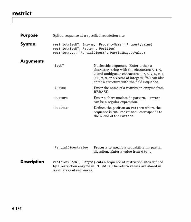
restrict
Purpose Split a sequence at a specified restriction site
Syntax restrict(SeqNT, Enzyme, 'PropertyName', PropertyValue)restrict(SeqNT, Pattern, Position)restrict(..., 'PartialDigest', PartialDigestValue)
ArgumentsSeqNT Nucleotide sequence. Enter either a
character string with the characters A, T, G,C, and ambiguous characters R, Y, K, M, S, W, B,D, H, V, N, or a vector of integers. You can alsoenter a structure with the field Sequence.
Enzyme Enter the name of a restriction enzyme fromREBASE.
Pattern Enter a short nucleotide pattern. Patterncan be a regular expression.
Position Defines the position on Pattern where thesequence is cut. Position=0 corresponds tothe 5’ end of the Pattern.
PartialDigestValue Property to specify a probability for partialdigestion. Enter a value from 0 to 1.
Description restrict(SeqNT, Enzyme) cuts a sequence at restriction sites definedby a restriction enzyme in REBASE. The return values are stored ina cell array of sequences.
6-186

restrict
REBASE, the restriction enzyme database, is a collection of informationabout restriction enzymes and related proteins. Search REBASE for thename of a restriction enzyme at
http://rebase.neb.com/rebase/rebase.html
For more information on REBASE, go to
http://rebase.neb.com/rebase/rebase.html
restrict(SeqNT, Pattern, Position) cuts a sequence at restrictionsites specified by a nucleotide pattern.
restrict(..., 'PartialDigest', PartialDigestValue) simulatesa partial digest where each restriction site in the sequence has aprobability PartilDigest of being cut.
Examples Use the recognition pattern (sequence) GCGC with the point of cleavageat position 3 to cleave a nucleotide sequence.
Seq = 'AGAGGGGTACGCGCTCTGAAAAGCGGGAACCTCGTGGCGCTTTATTAA';partsP = restrict(Seq,'GCGC',3);
partsP ='AGAGGGGTACGCG''CTCTGAAAAGCGGGAACCTCGTGGCG''CTTTATTAA'
Use the restriction enzyme HspAI (recognition sequence GCGC with thepoint of cleavage at position 1) to cleave a nucleotide sequence.
partsE = restrict(Seq,'HspAI')
partsE ='AGAGGGGTACG''CGCTCTGAAAAGCGGGAACCTCGTGG''CGCTTTATTAA'
6-187

restrict
See Also Bioinformatics Toolbox function seqshowwords
MATLAB function regexp
6-188

revgeneticcode
Purpose Get the reverse mapping for a genetic code
Syntax map = revgeneticcoderevgeneticcode(GeneticCode,
'PropertyName', PropertyValue)
revgeneticcode(..., 'Alphabet' AlphabetValue)revgeneticcode(..., 'ThreeLetterCodes', CodesValue)
ArgumentsGeneticCode Enter a code number or code name from the
table Genetic Code on page 6-189. If you use acode name, you can truncate the name to thefirst two characters of the name.
AlphabetValue Property to select the nucleotide alphabet.Enter either 'dna' or 'rna'. The defaultvalue is 'dna'.
CodesValue Property to select one- or three-letter aminoacid codes. Enter true for three-letter code orfalse for one-letter code.
Genetic Code
Code Number Code Name
1 Standard
2 Vertebrate Mitochondrial
3 Yeast Mitochondrial
6-189

revgeneticcode
Code Number Code Name
4 Mold, Protozoan, CoelenterateMitochondrial, andMycoplasma/Spiroplasma
5 Invertebrate Mitochondrial
6 Ciliate, Dasycladacean, and HexamitaNuclear
9 Echinoderm Mitochondrial
10 Euplotid Nuclear
11 Bacterial, and Plant Plastid
12 Alternative Yeast Nuclear
13 Ascidian Mitochondrial
14 Flatworm Mitochondrial
15 Blepharisma Nuclear
16 Chlorophycean Mitochondrial
21 Trematode Mitochondrial
22 Scenedesmus Obliquus Mitochondrial
23 Thraustochytrium Mitochondrial
Description revgeneticcode returns a structure containing reverse mappings forthe genetic code.
map = revgeneticcode returns a structure containing the reversemapping for the standard genetic code.
revgeneticcode(GeneticCode) returns a structure of the inversemapping for alternate genetic codes.
revgeneticcode(..., 'Alphabet' AlphabetValue) defines thenucleotide alphabet to use in the map.
6-190

revgeneticcode
revgeneticcode(..., 'ThreeLetterCodes', CodesValue) returns themapping structure with three-letter amino acid codes as field namesinstead of the default single-letter codes if ThreeLetterCodes is true.
Examples moldcode = revgeneticcode(4,'Alphabet','rna');wormcode = revgeneticcode('Flatworm Mitochondrial',...
'ThreeLetterCode',true);
map = revgeneticcode
map =Name: 'Standard'
A: {'GCT' 'GCC' 'GCA' 'GCG'}R: {'CGT' 'CGC' 'CGA' 'CGG' 'AGA' 'AGG'}N: {'AAT' 'AAC'}D: {'GAT' 'GAC'}C: {'TGT' 'TGC'}Q: {'CAA' 'CAG'}E: {'GAA' 'GAG'}G: {'GGT' 'GGC' 'GGA' 'GGG'}H: {'CAT' 'CAC'}I: {'ATT' 'ATC' 'ATA'}L: {'TTA' 'TTG' 'CTT' 'CTC' 'CTA' 'CTG'}K: {'AAA' 'AAG'}M: {'ATG'}F: {'TTT' 'TTC'}P: {'CCT' 'CCC' 'CCA' 'CCG'}S: {'TCT' 'TCC' 'TCA' 'TCG' 'AGT' 'AGC'}T: {'ACT' 'ACC' 'ACA' 'ACG'}W: {'TGG'}Y: {'TAT' 'TAC'}V: {'GTT' 'GTC' 'GTA' 'GTG'}
Starts: {'TAA' 'TAG' 'TGA'}
See Also Bioinformatics Toolbox functions aa2nt, baselookup, geneticcode,nt2aa
6-191

rna2dna
Purpose Convert an RNA sequence of nucleotides to a DNA sequence
Syntax SeqDNA = rna2dna(SeqRNA)
ArgumentsSeqRNA Nucleotide sequence for RNA. Enter a character string
with the characters A, C, U, G, and the ambiguousnucleotide bases N, R, Y, K, M, S, W, B, D, H, and V.
Description SeqDNA = rna2dna(SeqRNA) converts any uracil nucleotides in an RNAsequence into thymine (U–>T), and returns in the same format as DNA.For example, if the RNA sequence is an integer sequence then so isSeqRNA.
Examples rna2dna('ACGAUGAGUCAUGCUU')
ans =ACGATGAGTCATGCTT
See Also Bioinformatics Toolbox function dna2rna
MATLAB functions strrep, regexp
6-192

scfread
Purpose Read trace data from a SCF file
Syntax [Sample, Probability, Comments] = scfread('File')[A,C,T,G, ProbA, ProbC, ProbG, ProbT,Comments] = scfread ('File')
ArgumentsFile SCF formatted file. Enter a filename or a path and
filename.
Description scfread reads data from a SCF formatted file into a MATLAB structure.
[Sample, Probability, Comments] = scfread('File') reads an SCFformatted file and returns the sample data in the structure Sample,with fields A, C, T, G, probability data in the structure Probability,and comment information from the file in Comments.
[A,C,T,G, ProbA, ProbC, ProbG, ProbT, Comments] = scfread('File') reads an SCF formatted file and returns the sample data andprobabilities for nucleotides in separate variables.
SCF files store data from DNA sequencing instruments. Eachfile includes sample data, sequence information, and the relativeprobabilities of each of the four bases. For more information on SCFfiles, see
http://www.mrc-lmb.cam.ac.uk/pubseq/manual/formats_unix_2.html
Examples Examples of SCF files can be found at
ftp://ftp.ncbi.nih.gov/pub/TraceDB/example/
Unzip the file bcm-example.tgz with SCF files to your MATLABworking directory.
[Sample, Probability, Comments] = scfread('HCIUP1D61207.scf')
Sample =
6-193

scfread
A: [10827x1 double]C: [10827x1 double]G: [10827x1 double]T: [10827x1 double]
Probability =prob_A: [742x1 double]prob_C: [742x1 double]prob_G: [742x1 double]prob_T: [742x1 double]
Comments =
SIGN=A=121,C=103,G=119,T=82SPAC= 16.25PRIM=0MACH=Arkansas_SN312DYEP=DT3700POP5{BD}v2.mobNAME=HCIUP1D61207LANE=6GELN=PROC=RTRK=CONV=phred version=0.990722.hCOMM=SRCE=ABI 373A or 377
See Also Bioinformatics Toolbox functions genbankread, traceplot
6-194

select
Purpose Select tree branches and leaves in a phytree object
Syntax S = select(T)S = select(T, N)[S, Selleaves, Selbranches] = select(...)
S = select(..., 'Reference', ReferenceValue)S = select(..., 'Criteria', CriteriaValue)S = select(..., 'Threshold', ThresholdValue)S = select(..., 'Exclude', ExcludeValue)S = select(..., 'Propagate', PropagateValue)
ArgumentsTree Phylogenetic tree created with the function
phytree.
N Number of closest nodes to the root node.
ReferenceValue Property to select a reference point formeasuring distance.
CriteriaValue Property to select a criteria for measuringdistance.
ThresholdValue Property to select a distance value. Nodes withdistances below this value are selected.
ExcludeValue Property to remove (exclude) branch orleaf nodes from the output. Enter 'none','branchs', or 'leaves'. The default value is'none'.
PropagateValue Property to select propagating nodes towardthe leaves or the root.
Description S = select(Tree, N) returns a logical vector (S) of size [NumNodesx 1] indicating the N closest nodes to the root node of a phytreeobject (Tree) where NumNodes = NumLeaves + NumBranches. The firstcriterion select uses is branch levels, then patristic distance (also
6-195

select
known as tree distance). By default, select uses inf as the value of N,and select(Tree) returns a vector with values of true.
S = select(..., 'Reference', ReferenceValue) changes thereference point(s) to measure the closeness. Reference can be theroot (default) or leaves. When using leaves, a node can have multipledistances to its descendant leaves (nonultrametric tree). If this the case,select considers the minimum distance to any descendant leaf.
S = select(..., 'Criteria', CriteriaValue) changes the criteriaselect uses to measure closeness. If C = 'levels' (default), thefirst criterion is branch levels and then patristic distance. If C ='distance', the first criterion is patristic distance and then branchlevels.
S = select(..., 'Threshold', ThresholdValue) selects all thenodes where closeness is less than or equal to the threshold value V.Notice that you can also use either of the properties 'criteria' or'reference', if N is not specified, then N = infF; otherwise you canlimit the number of selected nodes by N.
S = select(..., 'Exclude', ExcludeValue) sets a postfilter thatexcludes all the branch nodes from S when E='branches' or all the leafnodes when E='leaves'. The default is 'none'.
S = select(..., 'Propagate', PropagateValue) activates apostfunctionality that propagates the selected nodes to the leaves whenP=='toleaves' or toward the root finding a common ancestor when P== 'toroot'. The default value is 'none'. P may also be 'both'. The'Propagate' property acts after the 'Exclude' property.
[S, Selleaves, Selbranches] = select(...) returns two additionallogical vectors, one for the selected leaves and one for the selectedbranches.
6-196

select
Examples % Load a phylogenetic tree created from a protein family:tr = phytreeread('pf00002.tree');
% To find close products for a given protein (e.g. vips_human):ind = getbyname(tr,'vips_human');[sel,sel_leaves] = select(tr,'criteria','distance',...
'threshold',0.6,'reference',ind);view(tr,sel_leaves)
% To find potential outliers in the tree, use[sel,sel_leaves] = select(tr,'criteria','distance',...
'threshold',.3,...'reference','leaves',...'exclude','leaves',...'propagate','toleaves');
view(tr,~sel_leaves)
See Also The Bioinformatics Toolbox functions phytree, phytreetool
phytree object methods pdist, get.
6-197

seq2regexp
Purpose Convert a sequence with ambiguous characters to a regular expression
Syntax seq2regexp(Seq)
ArgumentsSeq Nucleotide or amino acid sequence.
Nucleotide Conversions
NucleotideLetter Nucleotide
NucleotideLetter Nucleotide
A—A Adenosine S—[GC] (Strong)
C—C Cytosine W—[AT] (Weak)
G—G Guanine B—[GTC]
T—T Thymidine D—[GAT]
U—U Uridine H—[ACT]
R—[GA] (Purine) V—[GCA]
Y—[TC] (Pyrimidine) N—[AGCT] Any nucleotide
K—[GT] (Keto) - — - Gap ofindeterminatelength
M—[AC] (Amino) ?—? Unknown
Amino Acid Conversion
Amino Acid Letter Description
B—[DN] Aspartic acid orasparagine
6-198

seq2regexp
Amino Acid Letter Description
Z—[EQ] Glutamic acid orglutamine
X—[ARNDCQEGHILKMFPSTWYV] Any amino acid
Description seq2regexp(Seq) converts ambiguous nucleotide or amino acid symbolsin a sequence into a regular expression format using IUB/IUPAC codes.
Examples Convert a nucleotide sequence into a regular expression.
r = seq2regexp('ACWTMAN')
r =AC[AT]T[AC]A[AGCT]
See Also Bioinformatics Toolbox functions restrict, seqwordcount
MATLAB functions regexp, regexpi
6-199

seqcomplement
Purpose Calculate the complementary strand of a nucleotide sequence
Syntax SeqC = seqcomplement(SeqNT)
ArgumentsSeqNT Enter either a character string with the characters A,
T (U), G, C, and ambiguous characters R, Y, K, M, S, W,B, D, H, V, N, or a vector of integers. You can also entera structure with the field Sequence.
Description SeqC = seqcomplement(SeqNT) calculates the complementary strand(A–>T, C–>G, G–>C, T–>A) of a DNA sequence and returns a sequence inthe same format as SeqNT. For example, if SeqNT is an integer sequencethen so is SeqC.
Examples Return the complement of a DNA nucleotide sequence.
s = 'ATCG';seqcomplement(s)
ans =TAGC
See Also Bioinformatics Toolbox functions seqrcomplement, seqreverse
6-200

seqdisp
Purpose Format long sequence output for easy viewing
Syntax seqdisp(Seq)
seqdisp(..., 'Row', RowValue)seqdisp(..., 'Column', ColumnValue)seqdisp(..., 'HiddenNumbers', HiddenNumber)
ArgumentsSeq Nucleotide or amino acid sequence of
characters. Enter a character array, a FASTAfile name, a MATLAB structure with fieldsfrom GenBank or GenPept. Multiple sequencesare allowed.FASTA files can have the fileextensions fa, fasta, fas, fsa, and fst.
RowValue Property to select the length of each row. Enteran integer. The default length is 60.
ColumnValue Property to select the column width. Enter aninteger. The default column width is 10.
HiddenNumber Property to control displaying numbers at thestart of each row. Enter true to hide numbers.
Description seqdisp(Seq) prints a sequence (Seq) in rows with a default row lengthof 60 and a default column width of 10.
seqdisp(..., 'Row', RowValue) defines the length of each row for thedisplayed sequence.
seqdisp(..., ’Column’, ColumnValue) defines the column width of datafor the displayed sequence.
seqdisp(..., ’ShowNumbers’, ShowNumbers), when ShowNumbers is false,turns the position numbers at the start of each row off. The default is'true'.
6-201
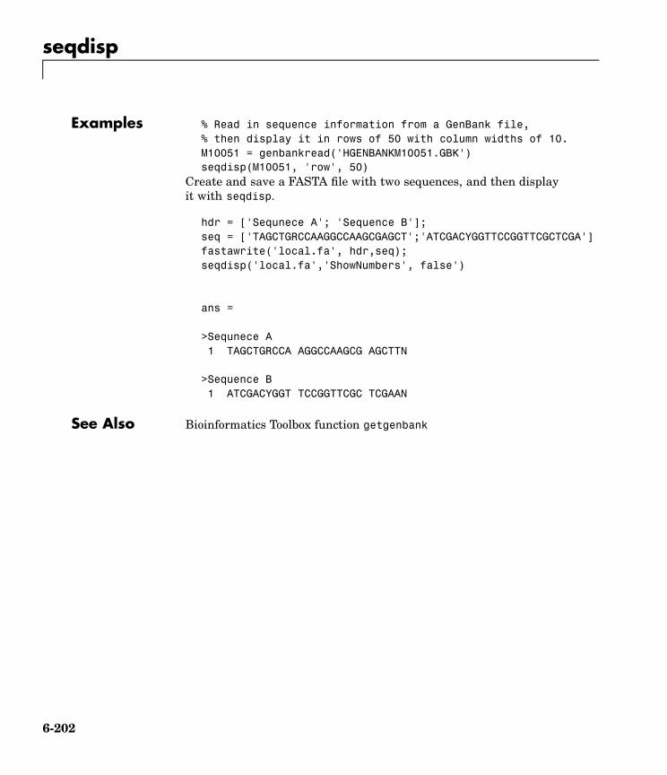
seqdisp
Examples % Read in sequence information from a GenBank file,% then display it in rows of 50 with column widths of 10.M10051 = genbankread('HGENBANKM10051.GBK')seqdisp(M10051, 'row', 50)
Create and save a FASTA file with two sequences, and then displayit with seqdisp.
hdr = ['Sequnece A'; 'Sequence B'];seq = ['TAGCTGRCCAAGGCCAAGCGAGCT';'ATCGACYGGTTCCGGTTCGCTCGA']fastawrite('local.fa', hdr,seq);seqdisp('local.fa','ShowNumbers', false')
ans =
>Sequnece A1 TAGCTGRCCA AGGCCAAGCG AGCTTN
>Sequence B1 ATCGACYGGT TCCGGTTCGC TCGAAN
See Also Bioinformatics Toolbox function getgenbank
6-202

seqdotplot
Purpose Create a dot plot of two sequences
Syntax seqdotplot(Seq1,Seq2)seqdotplot(Seq1,Seq2, Window, Number)
ArgumentsSeq1, Seq2 Nucleotide or amino acid sequences. Enter two
character strings. Do not enter a vector of integers.You can also enter a structure with the fieldSequence.
Window Enter an integer for the size of a window.
Number Enter an integer for the number of characterswithin the window that match.
Description seqdotplot (Seq1, Seq2) plots a figure that visualizes the matchbetween two sequences.
seqdotplot(Seq1,Seq2, Window, Number) plots sequence matcheswhen there are at least Number matches in a window of size Window.
When plotting nucleotide sequences, start with a Window of 11 andNumber of 7.
Matches = seqdotplot(...) returns the number of dots in the dotplot matrix.
[Matches, Matrix] = seqdotplot(...) = returns the dotplot as a sparsematrix.
Examples This example shows the similarities between the prion protein (PrP)nucleotide sequences of two ruminants, the moufflon and the goldentakin.
moufflon = getgenbank('AB060288','Sequence',true);takin = getgenbank('AB060290','Sequence',true);seqdotplot(moufflon,takin,11,7)
6-203

seqdotplot
Matches = seqdotplot(moufflon,takin,11,7)Matches =
5552
[Matches, Matrix] = seqdotplot(moufflon,takin,11,7)
See Also Bioinformatics Toolbox functions hmmprofalign, nwalign, swalign
6-204

seqlinkage
Purpose Construct a phylogenetic tree from pairwise distances
Syntax Tree = seqlinkage(Dist)Tree = seqlinkage(Dist, Method)Tree = seqlinkage(Dist, Method, Names)
ArgumentsDist Pairwise distances generated from the
function seqpdist.
Method Property to select a distance method. Entera method from the table below.
Names Property to use alternative labels for leafnodes. Enter a vector of structures, withthe fields 'Header' or 'Name', or a cellarray of strings. In both cases the numberof elements you provide must comply withthe number of samples used to generate thepairwise distances in Dist.
Description Tree = seqlinkage(Dist) returns a phylogenetic tree object from thepairwise distances (Dist) between the species or products. Dist is amatrix (or vector) such as is generated by the function seqpdist.
Tree = seqlinkage(Dist, Method) creates a phylogenetic tree objectusing a specified patristic distance method. The available methods are
'single' Nearest distance (single linkage method)
'complete' Furthest distance (complete linkage method)
'average' (default) Unweighted Pair Group Method Average(UPGMA, group average).
'weighted' Weighted Pair Group Method Average(WPGMA)
6-205

seqlinkage
'centroid' Unweighted Pair Group Method Centroid(UPGMC)
'median' Weighted Pair Group Method Centroid(WPGMC)
Tree = seqlinkage(Dist, Method, Names) passes a list of names tolabel the leaf nodes (for example, species or products) in a phylogenetictree object.
Examples % Load a multiple alignment of amino acids:seqs = fastaread('pf00002.fa');% Measure the 'Jukes-Cantor' pairwise distances:dist = seqpdist(seqs,'method','jukes-cantor',...
'indels','pair');% Build the phylogenetic tree with the single linkage% method and pass the names of the sequences:tree = seqlinkage(dist,'single',seqs)view(tree)
See Also The Bioinformatics Toolbox functions phytree, phytreewrite, seqpdist
phytree object methods plot and view
6-206

seqmatch
Purpose Find matches for every string in a library
Syntax Index = seqmatch(Strings, Library)
Description Index = seqmatch(Strings, Library) looks through the elements ofLibrary to find strings that begin with every string in Strings. Indexcontains the index to the first occurrence for every string in the query.Strings and Library must be cell arrays of strings.
Examples lib = {'VIPS_HUMAN', 'SCCR_RABIT', 'CALR_PIG' ,'VIPR_RAT', 'PACR_MOUSEquery = {'CALR','VIP'};h = seqmatch(query,lib);lib(h)
See Also MATLAB functions strmatch, regexpi
6-207
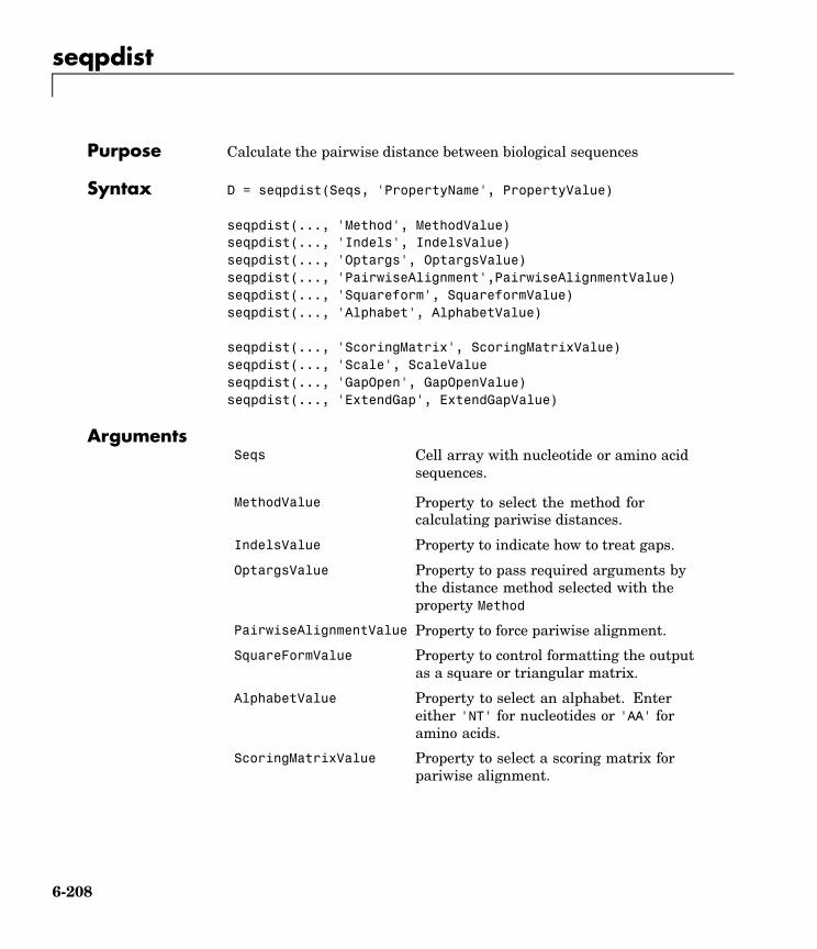
seqpdist
Purpose Calculate the pairwise distance between biological sequences
Syntax D = seqpdist(Seqs, 'PropertyName', PropertyValue)
seqpdist(..., 'Method', MethodValue)seqpdist(..., 'Indels', IndelsValue)seqpdist(..., 'Optargs', OptargsValue)seqpdist(..., 'PairwiseAlignment',PairwiseAlignmentValue)seqpdist(..., 'Squareform', SquareformValue)seqpdist(..., 'Alphabet', AlphabetValue)
seqpdist(..., 'ScoringMatrix', ScoringMatrixValue)seqpdist(..., 'Scale', ScaleValueseqpdist(..., 'GapOpen', GapOpenValue)seqpdist(..., 'ExtendGap', ExtendGapValue)
ArgumentsSeqs Cell array with nucleotide or amino acid
sequences.
MethodValue Property to select the method forcalculating pariwise distances.
IndelsValue Property to indicate how to treat gaps.
OptargsValue Property to pass required arguments bythe distance method selected with theproperty Method
PairwiseAlignmentValue Property to force pariwise alignment.
SquareFormValue Property to control formatting the outputas a square or triangular matrix.
AlphabetValue Property to select an alphabet. Entereither 'NT' for nucleotides or 'AA' foramino acids.
ScoringMatrixValue Property to select a scoring matrix forpariwise alignment.
6-208

seqpdist
ScaleValue Property to select a scale factor for thescoring matrix.
GapOpenValue Property to select a gap penalty.
ExtendGapValue Property to select a penalty for extendinga gap.
Description D = seqpdist(Seqs, 'PropertyName', PropertyValue) returns avector D containing biological distances between each pair of sequencesstored in the M elements of the cell Seqs.
D is an (M*(M-1)/2)-by-1 vector corresponding to the M*(M-1)/2pairs of sequences in Seqs. The output D is arranged in the order((2,1),(3,1),..., (M,1),(3,2),...(M,2),.....(M,M-1)). This isthe lower left triangle of the full M-by-M distance matrix. To get thedistance between the Ith and the Jth sequences for I > J, use theformula D((J-1)*(M-J/2)+I-J). Seqs can also be a vector of structureswith the field Sequence or a matrix of chars.
seqpdist(..., 'Method', MethodValue) selects the method seqpdistuses to compute the distances between every pair of sequences.
Distances defined for both nucleotides and amino acids:
'p-distance' Proportion of sites at which the two sequencesare different. p —> 1 for poorly related andp —> 0 for similar sequences.
'Jukes-Cantor'(default)
Maximum likelihood estimate of the numberof substitutions between two sequences. ForNT d = -3/4 log(1p * 4/3)
AA d = -19/20 log(1p * 20/19)
'alignment-score' Distance (d) between two sequences (1 and2) is computed from the pairwise alignmentscore (s) as follows:
d(1,2) = (1-s(1,2)/s(1,1))
6-209

seqpdist
* (1-s(1,2)/s(2,2))
This option does not imply that prealignedinput sequences will be realigned, itonly scores them. Use with care; thisdistance method does not comply with theultrametric condition. In the rare case wheres(x,y)>s(x,x), then d(x,y)=0.
Distances defined only for nucleotides and no scoring of gaps:
'Tajima-Nei' Maximum likelihood estimate consideringthe background nucleotide frequencies. Itcan be computed from the input sequencesor given by setting 'OPTARGS' to [gA gC gGgT].
'Kimura' Considers separately the transitional andtransversion nucleotide substitution.
'Tamura' Considers separately the transitional andtransversion nucleotide substitution and theGC content. GC content can be computedfrom the input sequences or given by setting'OPTARGS'.
6-210
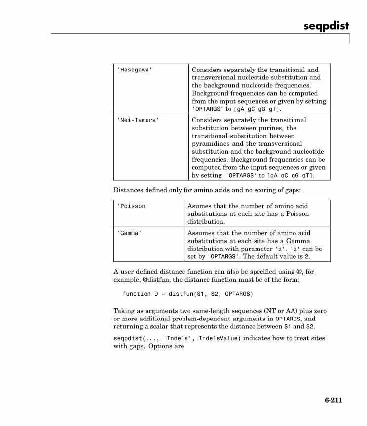
seqpdist
'Hasegawa' Considers separately the transitional andtransversional nucleotide substitution andthe background nucleotide frequencies.Background frequencies can be computedfrom the input sequences or given by setting'OPTARGS' to [gA gC gG gT].
'Nei-Tamura' Considers separately the transitionalsubstitution between purines, thetransitional substitution betweenpyramidines and the transversionalsubstitution and the background nucleotidefrequencies. Background frequencies can becomputed from the input sequences or givenby setting 'OPTARGS' to [gA gC gG gT].
Distances defined only for amino acids and no scoring of gaps:
'Poisson' Asumes that the number of amino acidsubstitutions at each site has a Poissondistribution.
'Gamma' Assumes that the number of amino acidsubstitutions at each site has a Gammadistribution with parameter 'a'. 'a' can beset by 'OPTARGS'. The default value is 2.
A user defined distance function can also be specified using @, forexample, @distfun, the distance function must be of the form:
function D = distfun(S1, S2, OPTARGS)
Taking as arguments two same-length sequences (NT or AA) plus zeroor more additional problem-dependent arguments in OPTARGS, andreturning a scalar that represents the distance between S1 and S2.
seqpdist(..., 'Indels', IndelsValue) indicates how to treat siteswith gaps. Options are
6-211

seqpdist
• 'score' (default) — Scores these sites either as a point mutation orwith the alignment parameters depending on the method selected.
• ’pairwise-del’ — For every pairwise comparison it ignores the siteswith gaps.
• ’complete-del’ — Ignores all the columns in the multiple alignmentthat contain a gap, this option is available only if a multiplealignment was provided at the input Seqs.
seqpdist(..., 'Optargs', OptargsValue) some distance methodsrequire or accept optional arguments. Use a cell array to pass morethan one input argument (for example, The nucleotide frequencies inthe Tajima-Nei distance function can be specified instead of computingthem from the input sequences).
seqpdist(..., 'PairwiseAlignment', PairwiseAlignmentValue),when PairwiseAlignment is true, ignores multiple alignment of theinput sequences (if any) and forces a pairwise alignment of inputsequences. If the input sequences are not prealigned, this flag is setautomatically. Pairwise alignment can be slow for a large number ofsequences. The default value is false.
seqpdist(..., 'Squareform', SquareformValue), when SquareFormis true, converts the output into a square formatted matrix so theD(I,J) denotes the distance between the Ith and Jth sequences.The output matrix is symmetric and has a zero diagonal. Settingthe property Squareform to true is the same as using the functionsquareform in the Statistical Toolbox.
seqpdist(..., 'Alphabet', AlphabetValue) specifies whether thesequences are amino acids ('AA') or nucleotides ('NT'). The defaultvalue is 'AA'.
The remaining input properties are analogous to the function nwalignand are used when the property PairwiseAlignment = true or theproperty Method = 'alignment-score'. For more information aboutthese properties, see nwalign.
6-212

seqpdist
seqpdist(..., 'ScoringMatrix', ScoringMatrixValue) specifiesthe scoring matrix to be used for the alignment. The default value isBLOSUM50 for AA and NUC44 for NT.
seqpdist(..., 'Scale', ScaleValue) indicates the scale factor of thescoring matrix to return the score using arbitrary units. If the scoringmatrix info also provides a scale factor, then both are used.
seqpdist(..., GapOpen', GapOpenValue) specifies the penalty foropening a gap in the alignment. The default gap open penalty is 8.
seqpdist(..., 'ExtendGap', ExtendGapValue) specifies the penaltyfor extending a gap in the alignment. If ExtendGap is not specified, thenextensions to gaps are scored with the same value as GapOpen.
Examples % Load a multiple alignment of amino acids:seqs = fastaread('pf00002.fa');
% For every possible pair of sequences in the multiple% alignment removes sites with gaps and scores with the% substitution matrix PAM250:
dist = seqpdist(seqs,'method','alignment-score',...'indels','pairwise-delete',...'scoringmatrix','pam250')
% To force the realignment of every pair of sequences% ignoring the provided multiple alignment:
dist = seqpdist(seqs,'method','alignment-score',...'indels','pairwise-delete',...'scoringmatrix','pam250',...'pairwisealignment',true)
% To measure the 'Jukes-Cantor' pairwise distances after% realigning every pair of sequences, counting the gaps as% point mutations:
6-213

seqpdist
dist = seqpdist(seqs,'method','jukes-cantor',...'indels','score',...'scoringmatrix','pam250',...'pairwisealignment',true)
See Also Bioinformatics Toolbox functions fastaread, seqlinkage
phytree methods phytree, pdist (phytree)
Statistical Toolbox functions pdist, squareform
6-214
seqrcomplement
Purpose Calculate the reverse complement of a nucleotide sequence
Syntax SeqRC = seqrcomplement(SeqNT)
ArgumentsSeqNT Nucleotide sequence. Enter either a character string
with the characters A, T (U), G, C, and ambiguouscharacters R, Y, K, M, S, W, B, D, H, V, N, or a vector ofintegers. You can also enter a structure with the fieldSequence.
Description seqrcomplement calculates the reverse complementary strand of aDNA sequence.
SeqRC = seqrcomplement(SeqNT) calculates the reverse complementarystrand 3' –> 5' (A–>T, C–>G, G–>C, T–>A) for a DNA sequence andreturns a sequence in the same format as SeqNT. For example, if SeqNTis an integer sequence then so is SeqRC.
Examples Reverse a DNA nucleotide sequence and then return its complement.
s = 'ATCG'seqrcomplement(s)
ans =CGAT
See Also Bioinformatics Toolbox functions codoncount, palindromesseqcomplement, seqreverse
6-215

seqreverse
Purpose Reverse the letters or numbers in a nucleotide sequence
Syntax SeqR = seqreverse(SeqNT)
ArgumentsSeqNT Enter a nucleotide sequence. Enter either a character
string with the characters A, T (U), G, C, and ambiguouscharacters R, Y, K, M, S, W, B, D, H, V, N, or a vector ofintegers. You can also enter a structure with the fieldSequence.
SeqR Returns a sequence in the same format as the nucleotidesequence. For example, if SeqNT is an integer sequence,then so is SeqR.
Description seqreverse calculates the reverse strand of a DNA or RNA sequence.
SeqR = seqreverse(SeqNT) calculates the reverse strand 3’ –> 5’ ofthe nucleotide sequence.
Examples Reverse a nucleotide sequence.
s = 'ATCG'seqreverse(s)
ans =GCTA
See Also Bioinformatics Toolbox functions seqcomplement, seqrcomplement
MATLAB function fliplr
6-216

seqshoworfs
Purpose Graphically display the open reading frames in a sequence
Syntax seqshoworfs(SeqNT, 'PropertyName', PropertyValue)
seqshoworfs(..., 'Frames', FramesValue)seqshoworfs(..., 'GeneticCode', GeneticCodeValue)seqshoworfs(..., 'MinimumLength', MinimumLengthValue)seqshoworfs(..., 'AlternativeStartCodons', StartCodonsValue)seqshoworfs(..., 'Color', ColorValue)seqshoworfs(..., 'Columns', ColumnsValue)
ArgumentsSeqNT Nucleotide sequence. Enter either a
character string with the characters A, T(U), G, C, and ambiguous characters R, Y, K,M, S, W, B, D, H, V, N, or a vector of integers.You can also enter a structure with the fieldSequence.
FramesValue Property to select the frame. Enter 1, 2, 3,-1, -2, -3, enter a vector with integers, or'all'. The default value is the vector [1 23]. Frames -1, -2, and -3 correspond to thefirst, second, and third reading frames for thereverse complement.
GeneticCodeValue Genetic code name. Enter a code number ora code name from the table geneticcode.
MinimumLengthValue Property to set the minimum number ofcodons in an ORF.
StartCodonsValue Property to control using alternative startcodons. Enter either true or false. Thedefault value is false.
6-217
seqshoworfs
ColorValue Property to select the color for highlightingthe reading frame. Enter either a 1-by-3 RGBvector specifying the intensity (0 to 255) ofthe red, green, and blue components of thecolor, or a character from the following list:'b'—blue, 'g'—green, 'r'—red, 'c'—cyan,'m'—magenta, or 'y'—yellow.
To specify different colors for the threereading frames, use a 1-by-3 cell array ofcolor values. If you are displaying reversecomplement reading frames, then COLORshould be a 1-by-6 cell array of color values.
ColumnsValue Property to specify the number of columnsin the output.
Description seqshoworfs identifies and highlights all open reading frames using thestandard or an alternative genetic code.
seqshoworfs(SeqNT) displays the sequence with all open readingframes highlighted, and it returns a structure of start and stop positionsfor each ORF in each reading frame. The standard genetic code is usedwith start codon 'AUG' and stop codons 'UAA', 'UAG', and 'UGA'.
seqshoworfs(..., 'Frames', FramesValue) specifies the readingframes to display. The default is to display the first, second, and thirdreading frames with ORFs highlighted in each frame.
seqshoworfs(..., 'GeneticCode', GeneticCodeValue) specifies thegenetic code to use for finding open reading frames.
seqshoworfs(..., 'MinimumLength', MinimumLengthValue) sets theminimum number of codons for an ORF to be considered valid. Thedefault value is 10.
seqshoworfs(..., 'AlternativeStartCodons', StartCodonsValue)uses alternative start codons if AlternativeStartCodons is set to true.For example, in the human mitochondrial genetic code, AUA and AUU are
6-218

seqshoworfs
known to be alternative start codons. For more details of alternativestart codons, see
http://www.ncbi.nlm.nih.gov/Taxonomy/Utils/wprintgc.cgi?mode=t#SG1
seqshoworfs(..., 'Color', ColorValue) selects the color used tohighlight the open reading frames in the output display. The defaultcolor scheme is blue for the first reading frame, red for the second, andgreen for the third frame.
seqshoworfs(..., 'Columns', ColumnsValue) specifies how manycolumns per line to use in the output. The default value is 64.
Examples Look for the open reading frames in a random nucleotide sequence.
s = randseq(200,'alphabet', 'dna');seqshoworfs(s);
Identify the open reading frames in a GenBank sequence.
HLA_DQB1 = getgenbank('NM_002123');seqshoworfs(HLA_DQB1.Sequence);
See Also Bioinformatics Toolbox functions codoncount, geneticcode,seqdisp,seqshowwords, seqwordcount
MATLAB function regexp
6-219
seqshowwords
Purpose Graphically display the words in a sequence
Syntax seqshowwords(Seq, Word, 'PropertyName', PropertyValue)
seqshowwords(...,'Color', ColorValue)seqshowwords(...,'Columns', ColumnsValue)
ArgumentsSeq Enter either a nucleotide or amino acid sequence.
You can also enter a structure with the fieldSequence.
Word Enter a short character sequence.
ColorValue Property to select the color for highlightedcharacters. Enter a 1-by-3 RGB vector specifyingthe intensity (0255) of the red, green, and bluecomponents, or enter a character from the followinglist: 'b'– blue, 'g'– green, 'r'– red, 'c'– cyan,'m'– magenta, or 'y'– yellow.
The default color is red 'r'.
ColumnsValue Property to specify the number of characters in aline. Default value is 64.
Description seqshowwords(Seq, Word) displays the sequence with all occurrencesof a word highlighted, and returns a structure with the start and stoppositions for all occurrences of the word in the sequence.
seqshowwords(...,'Color', ColorValue) selects the color used tohighlight the words in the output display.
seqshowwords(...,'Columns', ColumnsValue) specifies how manycolumns per line to use in the output.
Examples If word contains nucleotide or amino acid symbols that representmultiple possible symbols (ambiguous characters), then seqshowwordsshows all matches. For example, the symbol R represents either
6-220

seqshowwords
G or A (purines). For another example, if word equals 'ART', thenseqshowwords counts occurrences of both 'AAT' and 'AGT'. Thisexample shows two matches, ’TAGT' and 'TAAT', for the word 'BART'.
seqshowwords('GCTAGTAACGTATATATAAT','BART')
ans =Start: [3 17]Stop: [6 20]
000001 GCTAGTAACGTATATATAAT
seqshowwords does not highlight overlapping patterns multiple times.This example highlights two places, the first occurrence of 'TATA’and the 'TATATATA' immediately after 'CG'. The final 'TA' is nothighlighted because the preceding 'TA' is part of an already matchedpattern.
seqshowwords('GCTATAACGTATATATATA','TATA')
ans =Start: [3 10 14]Stop: [6 13 17]
000001 GCTATAACGTATATATATA
To highlight all multiple repeats of TA, use the regular expression'TA(TA)*TA'.
seqshowwords('GCTATAACGTATATATATA','TA(TA)*TA')
ans =Start: [3 10]Stop: [6 19]
000001 GCTATAACGTATATATATA
6-221

seqshowwords
See Also Bioinformatics Toolbox functions palindromes, restrict, seqdisp,seqshoworfs
MATLAB functions findstr, regexp
6-222

seqwordcount
Purpose Count the number of occurrences of a word in a sequence
Syntax seqwordcount(Seq, Word)
ArgumentsSeq Enter a nucleotide or amino acid sequence of characters.
You can also enter a structure with the field Sequence.
Word Enter a short sequence of characters.
Description seqwordcount(Seq, Word) counts the number of times that a wordappears in a sequence, and then returns the number of occurrences ofthat word.
If Word contains nucleotide or amino acid symbols that representmultiple possible symbols (ambiguous characters), then seqwordcountcounts all matches. For example, the symbol R represents eitherG or A (purines). For another example, if word equals 'ART', thenseqwordcount counts occurrences of both 'AAT' and 'AGT'.
Examples seqwordcount does not count overlapping patterns multiple times. Inthe following example, seqwordcount reports three matches. TATATATAis counted as two distinct matches, not three overlapping occurrences.
seqwordcount('GCTATAACGTATATATAT','TATA')
ans =3
The following example reports two matches ('TAGT' and 'TAAT'). Bis the ambiguous code for G, T, or C, while R is an ambiguous code forG and A.
seqwordcount('GCTAGTAACGTATATATAAT','BART')
ans =2
6-223

seqwordcount
See Also Bioinformatics Toolbox functions codoncount, seqshoworfs,seqshowwords
MATLAB functions seq2regexp, strfind
6-224

showalignment
Purpose Display a sequence alignment with color
Syntax showalignment(Alignment, 'PropertyName', PropertyValue)
showalignment(..., 'StartPointers', StartPointersValue)showalignment(..., 'MatchColor', MatchColorValue)showalignment(..., 'SimilarColor' SimilarColorValue)showalignment(..., 'Columns', ColumnsValue)
ArgumentsAlignment Enter the output from either the function
swalign or nwalign.
SimilarColorValue Property to specify the starting indices of thealigned sequences. StartPointers is the twoelement vector returned as the third outputof the function swalign.
MatchColorValue Property to select the color to highlightmatching characters. Enter a 1-by-N RGBvector specifying the intensity (0 to 255) ofthe red, green, and blue components, or entera character from the following list: 'b'–blue, 'g'– green, 'r'– red, 'c'– cyan, 'm'–magenta, or 'y'– yellow.
The default color is red, 'r'.
SimilarColorValue Property to select the color to highlightsimilar characters. Enter a 1-by-3 RGBvector or color character. The default coloris magenta.
ColumnsValue Property to specify the number of charactersin a line. Enter the number of characters todisplay in one row. The default value is 64.
6-225

showalignment
Description showalignment(Alignment, 'PropertyName', PropertyValue)displays an alignment string with matches and similar residueshighlighted with color.
showalignment(..., 'StartPointers', StartPointersValue)specifies the starting indices in the original sequences of a localalignment.
showalignment(..., 'MatchColor', MatchColorValue) selects thecolor to highlight the matches in the output display. The default color isred. For example, to use cyan, enter 'c' or [0 255 255].
showalignment(..., 'SimilarColor' SimilarColorValue) selectsthe color to highlight similar residues that are not exact matches. Thedefault color is magenta.
showalignment(..., 'Columns', ColumnsValue) specifies how manycolumns per line to use in the output, and labels the start of each rowwith the sequence positions.
Examples Enter two amino acid sequences and show their alignment.
[Score, Alignment] = nwalign('VSPAGMASGYD','IPGKASYD');showalignment(Alignment);
See Also Bioinformatics Toolbox functions nwalign, swalign
6-226

showhmmprof
Purpose Plot an HMM profile
Syntax showhmmprof(Model, 'PropertyName', PropertyValue)
showhmmprof(..., 'Scale', ScaleValue)
ArgumentsModel Hidden Markov model created with the functions
gethmmprof and pfamhmmread functions.
ScaleValue Enter one of the following values:
'logprob' — Log probabilities
'prob' — Probabilities
'logodds' — Log-odd ratios
Description showhmmprof(Model) plots a profile hidden Markov model described bythe structure Model.
showhmmprof(Model, 'Scale', ScaleValue) specifies the scaleto use. If log probabilities (ScaleValue='logprob'), probabilities(ScaleValue='prob'), or log-odd ratios (ScaleValue='logodds'). Tocompute the log-odd ratios, the null model probabilities are used forsymbol emission and equally distributed transitions are used for thenull transition probabilities. The default DomainValue is 'logprob'.
Examples load('hmm_model_examples','model_7tm_2') % load a model exampleshowhmmprof(model_7tm_2,'Scale','logodds')
See Also Bioinformatics Toolbox functions gethmmprof, hmmprofalign,hmmprofestimate, hmmprofgenerate, hmmprofstruct, pfamhmmread
6-227

sptread
Purpose Read data from a SPOT file
Syntax SPOTData = sptread('File','PropertyName', PropertyValue)
sptread(..., 'CleanColNames, 'CleanColNamesValues')
ArgumentsFile SPOT formatted file (ASCII text file).
Enter a filename, a path and filename, orURL pointing to a file. File can also bea MATLAB character array that containsthe text for a SPOT file.
CleanColNamesValue Property to control using valid MATLABvariable names.
Description SPOTData = sptread('File') reads a SPOT formatted file and createsa MATLAB structure SPOTData containing the following fields:
HeaderDataBlocksColumnsRowsIDsColumnNamesIndicesShape
sptread(..., 'CleanColNames, CleanColNamesValue) The columnnames in the SPOT file contain periods and some characters thatcannot be used in MATLAB variable names. If you plan to use thecolumn names as variable names in a function, use this option withCleanColNames set to true and the function will return the fieldColumnNames with valid variable names.
6-228

sptread
The Indices field of the structure includes the MATLAB indices thatyou can use for plotting heat maps of the data.
Examples % Read in a sample SPOT file and plot the median foreground% intensity for the 635 nm channel.spotStruct = sptread('spotdata.txt')maimage(spotStruct,'Rmedian');
% Alternatively, create a similar plot using% more basic graphics commands.
rmedCol = find(strcmp(spotStruct.ColumnNames,'Rmedian'));Rmedian = spotStruct.Data(:,rmedCol);imagesc(Rmedian(spotStruct.Indices));colormap bonecolorbar
See Also Bioinformatics Toolbox functions gprread, maimage
6-229

swalign
Purpose Locally align two sequences using the Smith-Waterman algorithm
Syntax [Score, Alignment] = swalign(Seq1, Seq2,'PropertyName', PropertyValue)
[Score, Alignment, Start] = swalign(Seq1, Seq2)
swalign(..., 'Alphabet', AlphabetValue)swalign(..., 'ScoringMatrix', ScoringMatrixValue)swalign(..., 'Scale', ScaleValue)swalign(..., 'GapOpen', GapOpenValue)swalign(..., 'ExtendGap', ExtendGapValue)
ArgumentsSeq1, Seq2 Nucleotide or amino acid sequences. Enter a
character string or vector of integers. You canalso enter a structure with the field Sequence.
AlphabetValue Property to select an amino acid or nucleotidesequences. Enter either 'AA' or 'NT'. Thedefault value is 'AA'.
ScoringMatrixValueEnter the name of a scoring matrix. Values are'PAM40’, 'PAM250', DAYHOFF, GONNET, 'BLOSUM30'increasing by 5 to 'BLOSUM90', or 'BLOSUM62',or 'BLOSUM100'.
The default value when AlphabetValue = 'aa'is 'BLOSUM50', while the default value whenAlphabeValue = 'nt' is nuc44.
ScaleValue Property to specify the scale factor for a scoringmatrix.
GapOpenValue Enter an integer for the gap penalty. Defaultvalue is 8.
ExtendGapValue Enter an integer for the extended gap penalty.The default value equals the GapOpen value.
6-230

swalign
Score Returns the alignment score. Units for Scoreare bits.
Alignment Returns a 3-by-n character array showing thetwo sequences and the alignment between them.
Start Position where the alignment begins in eachsequence.
Description [Score, Alignment] = swalign(Seq1, Seq2) returns a stringshowing an optimal local alignment for two amino acid sequences.Amino acids that match are indicated with the symbol |, while relatedamino acids (nonmatches with a positive scoring matrix value) areindicated with the symbol :.
[Score, Alignment, Start] = swalign(Seq1, Seq2) returns a 2-by-1vector with the starting point indices where the alignment begins foreach sequence.
swalign(...,'Alphabet', AlphabetValue) specifies whether thesequences are amino acids ('AA') or nucleotides ('NT'). The defaultvalue is 'AA'.
swalign(..., 'ScoringMatrix', ScoringMatrixValue) specifies thescoring matrix to use for the alignment. The default is 'blosum50' forAlphabet = 'AA' or 'NUC44' for Alphabet = NT.
swalign(..., 'Scale', ScaleValue) indicates the scale factor of thescoring matrix to return the score using arbitrary units. If the scoringmatrix also provides a scale factor, then both are used.
swalign(..., 'GapOpen', GapOpenValue) specifies the penalty foropening a gap in the alignment. The default gap open penalty is 8.
swalign(..., 'ExtendGap', ExtendGapValue) specifies the penaltyfor extending a gap in the alignment. If ExtendGap is not specified, thenextensions to gaps are scored with the same value as GapOpen.
6-231

swalign
Examples Return the score in bits and the local alignment using the defaultScoringMatrix ('BLOSUM50') and default values for the GapOpen andExtendGap values.
[Score, Alignment] = swalign('VSPAGMASGYD','IPGKASYD')
Score =8.6667
Alignment =PAGMASGYD| | || ||P-GKAS-YD
Align two amino sequences using a specified scoring matrix ('pam250')and a gap open penalty of 5.
[Score, Alignment] = swalign('HEAGAWGHEE','PAWHEAE',...'ScoringMatrix', 'pam250',...'GapOpen',5)
Score =8
Alignment =GAWGHE:|| ||PAW-HE
Align two amino sequences and return the Score in nat units (nats).
[Score, Alignment] = swalign('HEAGAWGHEE','PAWHEAE',...'Scale',log(2))
Score =6.4694
Alignment =AWGHE|| ||
6-232

swalign
AW-HE
See Also Bioinformatics Toolbox functions blosum, dayhoff, gonnet, nt2aa,nwalign, showalignment
6-233

traceplot
Purpose Draw nucleotide trace plots
Syntax traceplot(TraceStructure)traceplot(A, C, G, T)h = traceplot()
Description traceplot(TraceStructure) creates a trace plot from data in astructure with fields A, C, G, T.
traceplot(A, C, G, T) creates a trace plot from data in vectors A,C, G, T.
h = traceplot() returns a structure with the handles of the linescorresponding to A, C, G, T.
Examples tstruct = scfread('sample.scf');traceplot(tstruct)
See Also Bioinformatics Toolbox function scfread
6-234

view (phytree)
Purpose View a phylogenetic tree in the phytreetool window.
Syntax view(Tree)view(Tree, IntNodes)
ArgumentsTree phytree object created with phytree.
IntNodes Nodes form the phytree object to initiallydisplay in the Tree.
Description view(Tree) opens the Phylogenetic Tree Tool window and draws atree from data in a phytree object (Tree). The significant distancesbetween branches and nodes are in the horizontal direction. Verticaldistances have no significance and are selected only for display purposes.You can access tools to edit and analyze the tree from the PhylogeneticTree Tool menu bar or by using the left and right mouse buttons.
view(Tree, IntNodes) opens the Phylogenetic Tree Tool windowwith an initial selection of nodes specified by IntNodes. IntNodes can bea logical array of any of the following sizes: NumLeaves + NumBranchesx 1, NumLeaves x 1, or NumBranches x 1. IntNodes can also be a list ofindices.
Examples tr = phytreeread('pf00002.tree')view(tree)
See Also Bioinformatics Toolbox functions phytreeread, phytreetool,seqlinkage
phytree object methods phytree, plot (phytree)
6-235


A
Examples

A Examples
Sequence Analysis“Example: Sequence Statistics” on page 2-2“Example: Sequence Alignment” on page 2-17
A-2

Microarray Analysis
Microarray Analysis“Example: Visualizing Microarray Data” on page 3-2“Example: Analyzing Gene Expression Profiles” on page 3-25
A-3

A Examples
Phylogenetic Analysis“Example: Building a Phylogenetic Tree” on page 4-2
A-4

Index
Aamino acids
comparing sequences 2-27composition 2-14
applicationsdeploying 1-12prototyping 1-12
BBioinformatics Toolbox
computation with MATLAB 1-2defined 1-2expected user 1-4installation 1-5required software 1-5visualizing data 1-2
Cclusters
gene expression data 3-32codons
nucleotide composition 2-8composition
amino acid 2-14nucleotide 2-8
conversionsnucleotide to amino acid 2-14
Ddata
filtering microarray data 3-29getting into MATLAB 2-4loading into MATLAB 3-25microarray 3-3
data formatssupporting functions 1-7
databases
getting information from 2-19related genes 2-21supporting functions 1-7
Eexample
gene expression in mouse brain 3-2gene expression in yeast metabolism 3-25sequence alignment 2-17sequence statistics 2-2
Ffeatures
application deployment 1-12prototyping 1-12
functionsdata formats 1-7databases 1-7microarray analysis 1-10protein structure analysis 1-10sequence alignment 1-9sequence utilities 1-9
Ggene expression profile
mouse brain 3-2yeast metabolism 3-25
genome datawith MATLAB structures 3-25
Iinstallation
from CD or Web 1-5
MMATLAB structures
Index-1

Index
with genome data 2-4microarray
clustering genes 3-32filtering data 3-29mouse brain example 3-1principal component analysis 3-36scatter plots 3-16spacial images 3-5statistics 3-15visualizing data 3-2working with data 3-3yeast example 3-1
microarray analysissupporting functions 1-10
model organismfinding 2-17
mouse braingene expression profile 3-2microarray tutorial 3-2
NNCBI
searching Web site 2-17nucleotides
composition in sequences 2-5content in sequences 2-2searching database 2-21
Oopen reading frames
searching for 2-11
Pplots
scatter 3-16principal component analysis
filtering microarray data 3-36protein sequence
locating 2-24protein structure
analysis functions 1-10prototyping
supporting features 1-12
Ssequence
amino acid conversion 2-14codon composition 2-8comparing amino acids 2-27nucleotide content 2-2protein coding 2-24searching database 2-21statistics example 2-2
sequence alignmentexample 2-17supporting functions 1-9
sequence analysisdefined 2-1
sequence utilitiessupporting functions 1-9
sequencesnucleotide composition 2-5
share algorithmssupporting features 1-12
softwareadditional 1-5required 1-5
spatial imagesmicroarray 3-5
statisticsmicroarray 3-15
structureswith genome data 3-25
Vvisualizing data
Index-2

Index
microarray 3-2
Index-3