bioinformatics i fall 2003 copyright susan smith 1 phylogenetic analysis
Post on 19-Dec-2015
220 views
TRANSCRIPT

Bioinformatics I Fall 2003 copyright Susan Smith
1
Phylogenetic AnalysisPhylogenetic Analysis

Bioinformatics I Fall 2003 copyright Susan Smith
2
General comments on phylogeneticsGeneral comments on phylogenetics• Phylogenetics is the branch of
biology that deals with evolutionary relatedness
• Uses some measure of evolutionary relatedness: e.g., morphological features
• Phylogenetics is the branch of biology that deals with evolutionary relatedness
• Uses some measure of evolutionary relatedness: e.g., morphological features

Bioinformatics I Fall 2003 copyright Susan Smith
3
• Phylogenetics on sequence data is an attempt to reconstruct the evolutionary history of those sequences
• Relationships between individual sequences are not necessarily the same as those between the organisms they are found in
• Phylogenetics on sequence data is an attempt to reconstruct the evolutionary history of those sequences
• Relationships between individual sequences are not necessarily the same as those between the organisms they are found in

Bioinformatics I Fall 2003 copyright Susan Smith
4
• The ultimate goal is to be able to use sequence data from many sequences (and whole genomes) to give information about phylogenetic history of organisms
• Phylogenetic relationships usually depicted as trees, with branches representing ancestors of “children”; the bottom of the tree (individual organisms) are leaves. Individual branch points are nodes.

Bioinformatics I Fall 2003 copyright Susan Smith
5
Phylogenetic trees Phylogenetic trees
A B C Dtime
A rooted tree
A
B
C
D
An unrooted tree
time?

Bioinformatics I Fall 2003 copyright Susan Smith
6
• We will only consider binary trees: edges split only into two branches (daughter edges)
• rooted trees have an explicit ancestor; the direction of time is explicit in these trees
• unrooted trees do not have an explicit ancestor; the direction of time is undetermined in such trees
• Number of possible rooted or unrooted trees grows extremely fast

Bioinformatics I Fall 2003 copyright Susan Smith
7
• Terminal nodes correspond to data
• Internal nodes usually represent an inferred common ancestor
• Roots can be assigned to unrooted trees by using an outgroup
• Terminal nodes correspond to data
• Internal nodes usually represent an inferred common ancestor
• Roots can be assigned to unrooted trees by using an outgroup
Bioinformatics I Fall 2003 copyright Susan Smith
8
ExerciseExercise
• Draw all possible rooted and unrooted trees involving 3 species.
• Draw all possible unrooted and rooted trees involving 4 species
• Draw all possible rooted and unrooted trees involving 3 species.
• Draw all possible unrooted and rooted trees involving 4 species

Bioinformatics I Fall 2003 copyright Susan Smith
9
Types of phylogenetic analysis methodsTypes of phylogenetic analysis methods
• Phenetic: trees are constructed based on observed characteristics, not on evolutionary history
• Cladistic: trees are constructed based on fitting observed characteristics to some model of evolutionary history
• Phenetic: trees are constructed based on observed characteristics, not on evolutionary history
• Cladistic: trees are constructed based on fitting observed characteristics to some model of evolutionary history
Distancemethods
ParsimonyandMaximumLikelihoodmethods

Bioinformatics I Fall 2003 copyright Susan Smith
10
Sequence considerationsSequence considerations
• Mutations are not all equal• deleterious -- majority• advantageous – small minority• neutral – large minority?
• Mutation rates are not all equal• r = K/(2T) where r = rate, K =
number of substitutions per site, and T = time
• Mutations are not all equal• deleterious -- majority• advantageous – small minority• neutral – large minority?
• Mutation rates are not all equal• r = K/(2T) where r = rate, K =
number of substitutions per site, and T = time

Bioinformatics I Fall 2003 copyright Susan Smith
11
Synonymous vs. nonsynonymous substitutionsSynonymous vs. nonsynonymous substitutions• Synonymous – many substitutions at the
3rd position of codons are synonymous = don’t lead to amino acid change
• Nonsynonymous – substitutions that do lead to amino acid changes
• Where would you predict substitution rates to be highest? Lowest?
• Synonymous – many substitutions at the 3rd position of codons are synonymous = don’t lead to amino acid change
• Nonsynonymous – substitutions that do lead to amino acid changes
• Where would you predict substitution rates to be highest? Lowest?

Bioinformatics I Fall 2003 copyright Susan Smith
12
Mutation vs. substitutionMutation vs. substitution• Mutation is a change• Substitution is a change that has been preserved
through evolution (has passed through some selective pressures)
• Initial frequency q of a mutation in a population: q = 1/(2N) where N = number of diploid organisms in the population
• Most substitutions now seen must be approximately selectively neutral otherwise they would have disappeared
• Probability that a mutation will be lost by chance is 1 – q; probability that it will be fixed (take over) = q
• Mean time for new neutral mutation to be fixed is 4N generations
• Mutation is a change• Substitution is a change that has been preserved
through evolution (has passed through some selective pressures)
• Initial frequency q of a mutation in a population: q = 1/(2N) where N = number of diploid organisms in the population
• Most substitutions now seen must be approximately selectively neutral otherwise they would have disappeared
• Probability that a mutation will be lost by chance is 1 – q; probability that it will be fixed (take over) = q
• Mean time for new neutral mutation to be fixed is 4N generations
Bioinformatics I Fall 2003 copyright Susan Smith
13
Estimating substitutionsEstimating substitutions
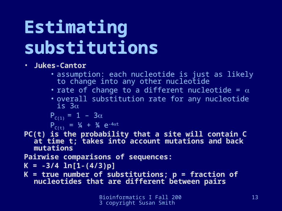
• Jukes-Cantor• assumption: each nucleotide is just as likely to change
into any other nucleotide• rate of change to a different nucleotide = • overall substitution rate for any nucleotide is 3PC(1) = 1 – 3PC(t) = ¼ + ¾ e-4t
PC(t) is the probability that a site will contain C at time t; takes into account mutations and back mutations
Pairwise comparisons of sequences:K = -3/4 ln[1-(4/3)p] K = true number of substitutions; p = fraction of nucleotides
that are different between pairs

Bioinformatics I Fall 2003 copyright Susan Smith
14
G
T C
A
C
C
C
C
T
CT=0
T=1
T=2
Bioinformatics I Fall 2003 copyright Susan Smith
15
Transitions and TransversionsTransitions and Transversions
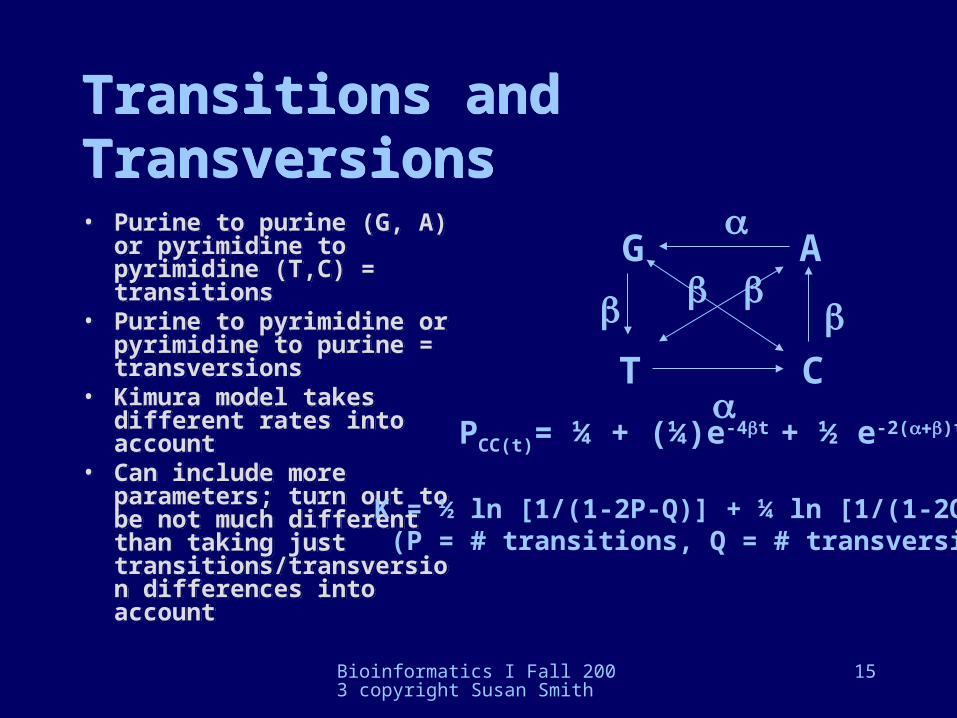
• Purine to purine (G, A) or pyrimidine to pyrimidine (T,C) = transitions
• Purine to pyrimidine or pyrimidine to purine = transversions
• Kimura model takes different rates into account
• Can include more parameters; turn out to be not much different than taking just transitions/transversion differences into account
G
T C
A
PCC(t)= ¼ + (¼)e-4t + ½ e-2()t
K = ½ ln [1/(1-2P-Q)] + ¼ ln [1/(1-2Q)] (P = # transitions, Q = # transversions)
Bioinformatics I Fall 2003 copyright Susan Smith
16
Distance methodsDistance methods
• Measuring distance -- just like when we talked about multiple alignment, distance represents all the differences at the various positions; these differences can be treated as equal or weighted according to empirical knowledge of substitution rates
• Measuring distance -- just like when we talked about multiple alignment, distance represents all the differences at the various positions; these differences can be treated as equal or weighted according to empirical knowledge of substitution rates

Bioinformatics I Fall 2003 copyright Susan Smith
17
• Another way to say this is that there are a set of distances dij between each pair of sequences i,j in the dataset. dij can be the fraction f of sites u where residues xi and xj differ; or dij can be such a fraction but weighted in some way (e.g. Jukes-Cantor distance)
• Another way to say this is that there are a set of distances dij between each pair of sequences i,j in the dataset. dij can be the fraction f of sites u where residues xi and xj differ; or dij can be such a fraction but weighted in some way (e.g. Jukes-Cantor distance)
Bioinformatics I Fall 2003 copyright Susan Smith
18
Clustering algorithmsClustering algorithms
• UPGMA = unweighted pair group method with arithmetic mean -- this is the distance clustering method that is used in pileup to make the guide tree (also the method for clustering other data …)
• Computes all the pairwise distances, joins the smallest two into a group, recomputes, etc.
• UPGMA = unweighted pair group method with arithmetic mean -- this is the distance clustering method that is used in pileup to make the guide tree (also the method for clustering other data …)
• Computes all the pairwise distances, joins the smallest two into a group, recomputes, etc.

Bioinformatics I Fall 2003 copyright Susan Smith
19
• Branch lengths can be computed from the distance matrix, assuming rates of evolution equal
• The branch length is just half of the distance between the two nodes (each branch gets half the total distance)
• Branch lengths can be computed from the distance matrix, assuming rates of evolution equal
• The branch length is just half of the distance between the two nodes (each branch gets half the total distance)

Bioinformatics I Fall 2003 copyright Susan Smith
20
ExerciseExercise
• Using given data, generate a pairwise distance matrix, join the first group, recompute, and iterate until you have a set of matrices that will allow you to create a tree.
• Estimate the branch lengths of your tree.
• Using given data, generate a pairwise distance matrix, join the first group, recompute, and iterate until you have a set of matrices that will allow you to create a tree.
• Estimate the branch lengths of your tree.

Bioinformatics I Fall 2003 copyright Susan Smith
21
Problems with UPGMAProblems with UPGMA
• UPGMA assumes a molecular clock mechanism of evolution
• This can be, but is not always, a reasonable assumption
• One indication that this is not a reasonable assumption is that branch lengths of UPGMA-generated trees do not add up to the predicted values
• UPGMA assumes a molecular clock mechanism of evolution
• This can be, but is not always, a reasonable assumption
• One indication that this is not a reasonable assumption is that branch lengths of UPGMA-generated trees do not add up to the predicted values

Bioinformatics I Fall 2003 copyright Susan Smith
22
• Taking different evolutionary rates into account is possible using the transformed distance method, and the neighbor-joining method
• Transformed distance method: use an outgroup, which you say diverged from all the other groups before they diverged from each other
• d’ij = (dij – diD – djD)/2 + dDav

Bioinformatics I Fall 2003 copyright Susan Smith
23
• Neighbor-joining: corrects for UPGMA’s assumption of the same rate of evolution for each branch by modifying the distance matrix to reflect different rates of change
• Covered very well in text
• Neighbor-joining: corrects for UPGMA’s assumption of the same rate of evolution for each branch by modifying the distance matrix to reflect different rates of change
• Covered very well in text

Bioinformatics I Fall 2003 copyright Susan Smith
24
PAUP tutorialPAUP tutorial• We will now follow some of the Quick-start tutorial instructions for using PAUP on
the command line• Log in to the server as usual• To see the tutorial:
– Hartford: In a unix window, type acroread /local/paup/Docs/Quick_start_v1.pdf
– Troy: open a unix window FROM YOUR SERVER DIRECTORY, then typeacroread Quick_start_v1.pdf
• Still from the server, in a different window, typepaup
• Follow instructions for “Portable”. The sample data set should just be in your directory so you shouldn’t have to change directories. You don’t really need to stop logging when the tutorial covers that. You also don’t need to actually do the “recall assumptions” part on p.9. Follow the directions until you get to page 11
• When you get to that section, skip ahead to “Setting the optimality criterion to distance” on p.16
• Follow the directions on p.16; when you get to p. 17, typeUPGMA;
(don’t type nj)• Examine the tree
• We will now follow some of the Quick-start tutorial instructions for using PAUP on the command line
• Log in to the server as usual• To see the tutorial:
– Hartford: In a unix window, type acroread /local/paup/Docs/Quick_start_v1.pdf
– Troy: open a unix window FROM YOUR SERVER DIRECTORY, then typeacroread Quick_start_v1.pdf
• Still from the server, in a different window, typepaup
• Follow instructions for “Portable”. The sample data set should just be in your directory so you shouldn’t have to change directories. You don’t really need to stop logging when the tutorial covers that. You also don’t need to actually do the “recall assumptions” part on p.9. Follow the directions until you get to page 11
• When you get to that section, skip ahead to “Setting the optimality criterion to distance” on p.16
• Follow the directions on p.16; when you get to p. 17, typeUPGMA;
(don’t type nj)• Examine the tree

Bioinformatics I Fall 2003 copyright Susan Smith
25
Parsimony methodsParsimony methods• Parsimony methods are based on the
idea that the most probable evolutionary pathway is the one that requires the smallest number of changes from some ancestral state
• For sequences, this implies treating each position separately and finding the minimal number of substitutions at each position
• Parsimony methods are based on the idea that the most probable evolutionary pathway is the one that requires the smallest number of changes from some ancestral state
• For sequences, this implies treating each position separately and finding the minimal number of substitutions at each position

Bioinformatics I Fall 2003 copyright Susan Smith
26
Informative vs. uninformative positionsInformative vs. uninformative positions• Informative sites allow some of the
possible trees to distinguished from the others on the basis of how many mutations they must invoke
• Obviously uninformative sites: all the same character at that site
• Less-obviously uninformative site: one substitution only
• Less-obviously uninformative site: less than two different characters, each character appears less than twice
• Informative sites allow some of the possible trees to distinguished from the others on the basis of how many mutations they must invoke
• Obviously uninformative sites: all the same character at that site
• Less-obviously uninformative site: one substitution only
• Less-obviously uninformative site: less than two different characters, each character appears less than twice
Bioinformatics I Fall 2003 copyright Susan Smith
27
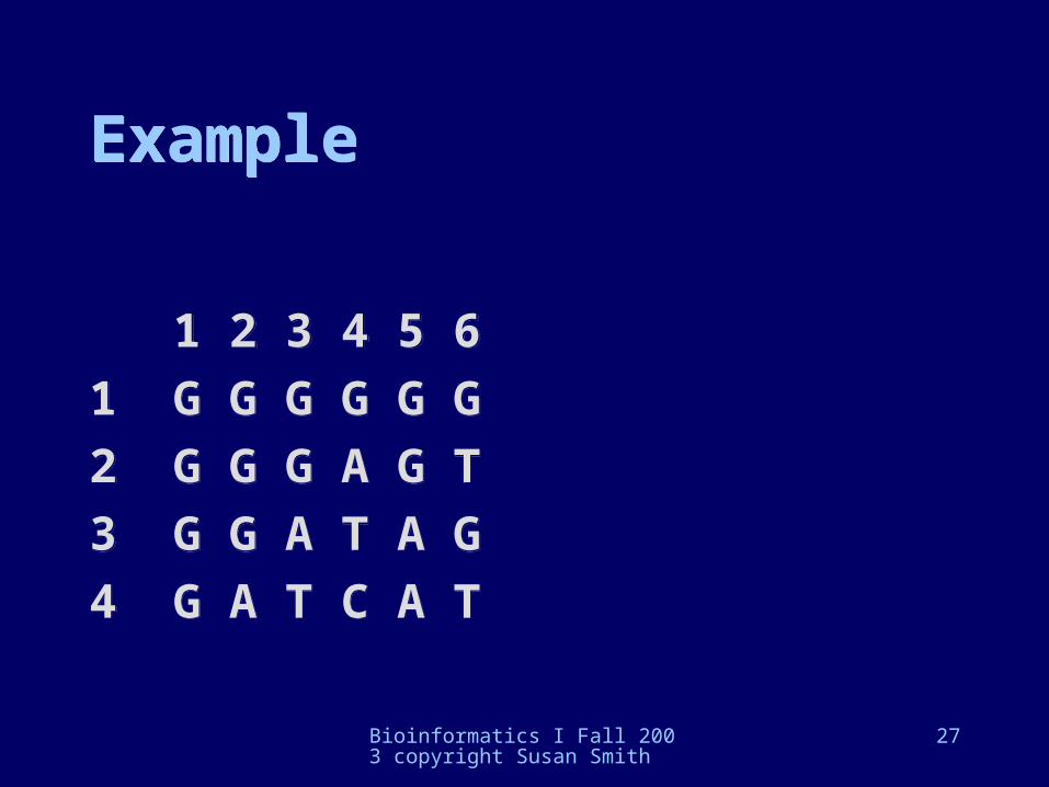
ExampleExample
1 2 3 4 5 6
1 G G G G G G
2 G G G A G T
3 G G A T A G
4 G A T C A T
1 2 3 4 5 6
1 G G G G G G
2 G G G A G T
3 G G A T A G
4 G A T C A T
Bioinformatics I Fall 2003 copyright Susan Smith
28
Parsimony uses only the informative sitesParsimony uses only the informative sites• The most parsimonious tree is the
one that invokes the fewest substitutions at informative sites
• Scoring means counting the number of substitutions needed
• There can be several trees with different topology that are equivalently parsimonious …
• The most parsimonious tree is the one that invokes the fewest substitutions at informative sites
• Scoring means counting the number of substitutions needed
• There can be several trees with different topology that are equivalently parsimonious …

Bioinformatics I Fall 2003 copyright Susan Smith
29
Example of parsimonious tree building Example of parsimonious tree building • Tree on left
requires only one change, tree on left requires two: left tree is most parsimonious
• Tree on left requires only one change, tree on left requires two: left tree is most parsimonious
Bioinformatics I Fall 2003 copyright Susan Smith
30
• Parsimony methods assign a cost to each tree available to the dataset, then screen trees available to the dataset and select the most parsimonious
• Screening all the trees available to even a smallish dataset would take too much time;
• branch and bound method
• Parsimony methods assign a cost to each tree available to the dataset, then screen trees available to the dataset and select the most parsimonious
• Screening all the trees available to even a smallish dataset would take too much time;
• branch and bound method

Bioinformatics I Fall 2003 copyright Susan Smith
31
• Can weight the cost to correspond with things known about the data – e.g., transitions occur more frequently than transversions
• You can inspect the dataset to be used to get the values of the weights to be used …
• Can weight the cost to correspond with things known about the data – e.g., transitions occur more frequently than transversions
• You can inspect the dataset to be used to get the values of the weights to be used …
Bioinformatics I Fall 2003 copyright Susan Smith
32
Parsimony is fundamentally different from UPGMAParsimony is fundamentally different from UPGMA
• It is not based on a distance, but on a presumed evolutionary path to an outcome
• One of the best ways to decide if a topology is well-supported is to compare trees generated by these two kinds of methods
• It is not based on a distance, but on a presumed evolutionary path to an outcome
• One of the best ways to decide if a topology is well-supported is to compare trees generated by these two kinds of methods
Bioinformatics I Fall 2003 copyright Susan Smith
33
In-class exercise IIIn-class exercise II
• Return to the PAUP tutorial, and this time follow the directions for using parsimony as the optimality criterion starting on p. 16.
• To see your tree, you will have to type
showtrees;
• Inspect your tree. Compare it to the distance generated tree.
• Return to the PAUP tutorial, and this time follow the directions for using parsimony as the optimality criterion starting on p. 16.
• To see your tree, you will have to type
showtrees;
• Inspect your tree. Compare it to the distance generated tree.

Bioinformatics I Fall 2003 copyright Susan Smith
34
Maximum likelihood methodsMaximum likelihood methods• Maximum likelihood reconstructs a
tree according to an explicit model of evolution. For the given model, no other method will work as well
• But, such models must be simple, because the method is computationally intensive
• Maximum likelihood reconstructs a tree according to an explicit model of evolution. For the given model, no other method will work as well
• But, such models must be simple, because the method is computationally intensive
Bioinformatics I Fall 2003 copyright Susan Smith
35
• Actually, all the other methods discussed implicitly use a simple model of evolution similar to the typical model made explicit in maximum likelihood:
• All sites selectively neutral
• All mutate independently, forward and reverse rates equal, given by
• Actually, all the other methods discussed implicitly use a simple model of evolution similar to the typical model made explicit in maximum likelihood:
• All sites selectively neutral
• All mutate independently, forward and reverse rates equal, given by

Bioinformatics I Fall 2003 copyright Susan Smith
36
• Maximum likelihood is maybe the “gold standard” for phylogenetic analysis; but because of its computational intensity it can only be used for select data and only after much initial fine tuning of many parameters of sequence alignments
• Often used to distinguish between several already generated trees

Bioinformatics I Fall 2003 copyright Susan Smith
37
• DO NOT USE MAXIMUM LIKELIHOOD TO BUILD TREES, TODAY OR FOR YOUR PROJECT.
• PLEASE!
• DO NOT USE MAXIMUM LIKELIHOOD TO BUILD TREES, TODAY OR FOR YOUR PROJECT.
• PLEASE!
Bioinformatics I Fall 2003 copyright Susan Smith
38
Assessing treesAssessing trees
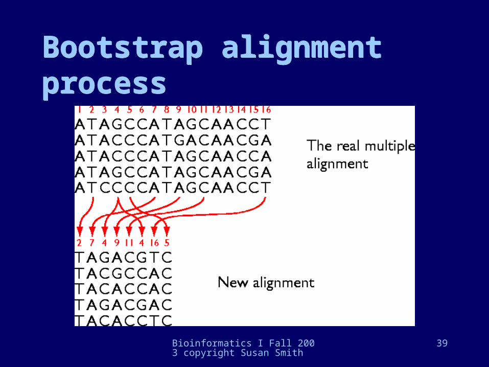
• The bootstrap: randomly sample all positions (columns in an alignment) with replacement -- meaning some columns can be repeated -- but conserving the number of positions; build a large dataset of these randomized samples
• The bootstrap: randomly sample all positions (columns in an alignment) with replacement -- meaning some columns can be repeated -- but conserving the number of positions; build a large dataset of these randomized samples
Bioinformatics I Fall 2003 copyright Susan Smith
39
Bootstrap alignment processBootstrap alignment process

Bioinformatics I Fall 2003 copyright Susan Smith
40
• Then use your method (distance, parsimony, likelihood) to generate another tree
• Do this a thousand or so times • Note that if the assumptions the method is
based on hold, you should always get the same tree from the bootstrapped alignments as you did originally
• The frequency of some feature of your phylogeny in the bootstrapped set gives some measure of the confidence you can have for this feature

Bioinformatics I Fall 2003 copyright Susan Smith
41
Protein sequences and phylogenetic analysisProtein sequences and phylogenetic analysis• Despite the fact that DNA sequences have more
characters (and contain more information), phylogenetic analysis is often done with protein sequences
• For your project, you can use either nucleic acids or proteins
• To do a phylogenetic analysis, you must start with a good MSA
• You will probably not want to use the whole length sequences, but instead use sections of the alignment that are 50 – 200 characters long
• For modular genes/proteins, it might be interesting to look at the trees made by aligned sections from the different modules …
• Despite the fact that DNA sequences have more characters (and contain more information), phylogenetic analysis is often done with protein sequences
• For your project, you can use either nucleic acids or proteins
• To do a phylogenetic analysis, you must start with a good MSA
• You will probably not want to use the whole length sequences, but instead use sections of the alignment that are 50 – 200 characters long
• For modular genes/proteins, it might be interesting to look at the trees made by aligned sections from the different modules …

Bioinformatics I Fall 2003 copyright Susan Smith
42
Running paup on protein MSA’sRunning paup on protein MSA’s• Find the file called phylo10.msf in my
directory; copy it to your directory
• view this file in seqlab’s editor
• start the paup program
• type the command (all on one line)tonexus format=gcg fromfile=phylo10.msf
tofile=phylo10.nex
• Find the file called phylo10.msf in my directory; copy it to your directory
• view this file in seqlab’s editor
• start the paup program
• type the command (all on one line)tonexus format=gcg fromfile=phylo10.msf
tofile=phylo10.nex

Bioinformatics I Fall 2003 copyright Susan Smith
43
• Execute the file• Then run distance tree, bootstrapped
• must use ‘total’ or ‘mean’ as the distance measure for proteins
dset distance=total
dset distance=mean• to see a bootstrapped tree for distance,
type
boot
• Execute the file• Then run distance tree, bootstrapped
• must use ‘total’ or ‘mean’ as the distance measure for proteins
dset distance=total
dset distance=mean• to see a bootstrapped tree for distance,
type
boot

Bioinformatics I Fall 2003 copyright Susan Smith
44
Then run a parsimony tree, bootstrapped
remember to change criterion, then you can use boot again
When the prompt asks you if you want to change the number of trees looked at, say no; then wait for the output
• just one or two groups per classroom should do this
• may take a few minutes
Then run a parsimony tree, bootstrapped
remember to change criterion, then you can use boot again
When the prompt asks you if you want to change the number of trees looked at, say no; then wait for the output
• just one or two groups per classroom should do this
• may take a few minutes
Bioinformatics I Fall 2003 copyright Susan Smith
45
Making a section of an alignmentMaking a section of an alignment• Find an area (50-100 characters long) of
the MSA that has few gaps• Select all the sequences’ names• Select everything up to the first character
of the section using Edit select range; cut the selected area
• Repeat, only select everything after the last character of the selection and cut that selection
• Find an area (50-100 characters long) of the MSA that has few gaps
• Select all the sequences’ names• Select everything up to the first character
of the section using Edit select range; cut the selected area
• Repeat, only select everything after the last character of the selection and cut that selection

Bioinformatics I Fall 2003 copyright Susan Smith
46
• Save the file as something you can remember
• This file must be made into a nexus file before you can use it in PAUP (tonexus etc.)
• Save the file as something you can remember
• This file must be made into a nexus file before you can use it in PAUP (tonexus etc.)