biofouling in membrane bioreactors: nexus between ... · nexus between polyacrylonitrile surface...

Biofouling in membrane bioreactors: Nexus between polyacrylonitrile surface charge and

community composition Biofouling in membraanbioreactoren:

Nexus tussen polyacrylonitrile oppervlaktelading en gemeenschapssamenstelling

juni 2015

Promotoren:

Prof. Ivo Vankelecom

Departement Microbiële en Moleculaire Systemen

Centrum voor Oppervlaktechemie en Katalyse

Prof. Dirk Springael

Departement Aard- en Omgevingswetenschappen

Afdeling Bodem- en Waterbeheer

Masterproef voorgedragen

tot het behalen van het diploma van

Master of science in de bio-ingenieurswetenschappen:

milieutechnologie

Marie-Aline Hernalsteens

"Dit proefschrift is een examendocument dat na de verdediging niet meer werd gecorrigeerd

voor eventueel vastgestelde fouten. In publicaties mag naar dit proefwerk verwezen worden

mits schriftelijke toelating van de promotor, vermeld op de titelpagina."

I

Acknowledgments

The very first person I have to sincerely thank is Louise Vanysacker, former Postdoc at the KU Leuven

and currently working at De Watergroep: eventually she was not part of this adventure, but she

convinced me to have a go with it and she could not be more right. Moreover Louise reviewed my

work externally in the very end and gave me valuable advice on the content.

I thank my promotor, Prof. Dhr. Ivo Vankelecom (Centre for Surface Chemistry and Catalysis, COK), and

my co-promotor, Prof. Dhr. Dirk Springael (Division of Soil and Water Management), for believing in

me in the first place, as well as for their contribution to constructive insights during the whole year.

My supervisors, the PhD students Shazia Ilyas and Lisendra Marbelia (COK) and the Postdoc Basak

Ozturk (Division of Soil and Water Management), have done a wonderful job. Shazia and Lisendra,

thank you for your (technical) support when you took over the maintenance of the bioreactor in my

absence and for the follow-up of the (external) membrane performance measurements. Basak, thank

you for your support. But most important, thank you for being that passionate about all you do and

demanding towards me. And you know, from the Destiny’s Child, you are Beyoncé, without doubt .

Thank you to the external evaluators Prof. Dr. ir. Kristel Bernaerts (Department of Chemical

Engineering) and Prof. Dhr. Koenraad Muylaert (Faculteit Wetenschappen @ Campus Kulak Kortrijk)

for assessing my work.

Next I would like to thank all people who helped or informed me on measurement techniques or gave

me their support during experiments.

First I need to thank the staff of Bonte Ateliers Leuven for providing me in good quality PVC membrane

frames.

I would like to thank Pedro, the cleaning man, for keeping our workspace tidy at every moment of the

week and for the delicious sweets he baked.

From the COK group, I would like to thank warmly Werner Wouters, highly skilled technician, for

helping me improving the bioreactor set-up. Thank you to Matthias Mertens, doctorate student, for

his general good mood and ready-to-help behaviour (i.a., during my quest for glutaraldehyde). Next I

want to thank Maarten Bastin for his unconditional devotion when it comes to SEM measurements in

II

the early morning. Finally I thank Dirk Dom for explaining me the functioning of the vacuum oven,

Nithya Joseph for explaining me high-throughput and SEM equipment and Hanne Mariën for giving me

her advice on the quality of my hand-made membranes.

From the Division of Soil and Water Management group, I would like to thank Dries Grauwels,

marathon laboratory technician, for the numerous bump-into-you moments. I thank Karla Moors,

laboratory technician, but in particular Lynn Lemoine, doctorate student, for their precious advice

during DGGE measurements and support when I needed it most. Also Benjamin Horemans is part of

this rather extended acknowledgments list for having performed remarkable CLSM measurements in

my company and for his help showing me around in the laboratory. Finally I thank Karlien Cassaert, the

secretary, for ordering the products most needed for the experiments, and for helping all master

thesis students organizing the fantastic Jungle party in December 2014.

From the Department of Chemical Engineering, I would like to thank Liesel Cluyts for technical support

during Hach Lange measurements and for guiding in the laboratories. I also need to thank Prof. Dr. ir.

Ilse Smets for giving me advice concerning bulking problems of the bioreactor, as well as Prof. Dr. ir.

Kristel Bernaerts for helping me in the completion of the Hach-Lange risk analysis forms. Finally I want

to thank Hassan Farrokhzad, PhD student, for his support during CAM measurements.

From the Department of Physics and Astronomy, I sincerely thank Prof. Dhr. Alexander Volodin for the

energy he has put into the countless AFM measurements.

From the Department of Materials Engineering I am grateful towards Gregory Pyka and Oksana

Shishkina for the time they spent looking for potential porometry measurement improvements on my

samples on an unselfish way.

From the Institut des Sciences Chimiques de Rennes I thank Prof. Dhr. Anthony Szymczyk for the zeta

potential measurements he performed with tremendous rapidity.

I finally thank from my heart my friends, namely the master thesis students Claudia Moens, Marieke

Verbeke, Steffie Evers, Mathias Nijsen and Kris Dox, without whom this adventure would not have

taken place, as well as the radiant master thesis student Marie Mulier, with whom I had the most

intense peptalks and data exchange. And in the very end I thank my lovely family for encouraging me

on staying on track by means of delicious meals, comforting arms and positive conversations.

III

Abstract

The membrane bioreactor (MBR) technology can now be considered a well-established alternative

wastewater treatment system to conventional techniques (CASP). Advantages comprise the delivery of

higher effluent quality as well as the smaller footprint requirement. However, aside from the high

investment cost, one of the main drawbacks and research challenges of membrane technology is

membrane fouling. Due to membrane fouling the performance of the filtration process decreases with

time, which implies high energy demands and operational costs related to fouling prevention,

mitigation and remediation. Example studies on membrane fouling in view of process optimization are

manifold, but there still exists a lack of knowledge about the microorganisms taking part in the fouling

process (i.e., biofouling) and their specific relation to the membrane surface chemistry and to the

wastewater environment. Thus this slows down the development of more targeted anti-(bio)fouling

strategies.

The purpose of this study was to elucidate the relationship between the specific surface charge

(neutral, positive, negative) of polyacrylonitrile (PAN) membranes and the development and

composition of the microbial community in the biofouling layer developed during 40 days in a

submerged laboratory-scale aerobic membrane bioreactor (HT-MBR) operated on protamylasse feed.

The work was performed using 13 wt% pure PAN membranes as well as 11 wt% PAN membranes

having undergone surface modifications (hydrolysis, layer-by-layer deposition of poly(allyl amine

hydrochloride) (PAH) and poly(acrylic acid) (PAA)). The synthesized membranes were analyzed

thoroughly in term of their physico-chemical properties (via ATR-FTIR, SEM, AFM, CAM, volume

porosity measurement, electrokinetic characterization) and their permeability/filterability (via CWP,

critical flux). The membrane biofouling was characterized based on molecular techniques (PCR-DGGE)

and physico-chemical techniques (via ATR-FTIR, SEM, CLSM).

The results revealed that the synthesized ultrafiltration (UF) membranes were only different in their

charges and chemical composition (due to functionalization) but not in pore size, porosity, clean water

permeability or surface roughness. This it allowed the fouling experiments to be solely determined by

these differences. Fingerprinting analysis indicated selective enrichment of bacterial populations from

the sludge suspension within the biofilms at any time point. Biofilm community composition seemed

to change with time. But since no difference was observed between the biofilm community of

different membranes at specific time points, it could be concluded that the local characteristics of the

membrane (here: charge) do not play a decisive role on the long term selection of the key foulants.

Enhanced knowledge on the specific relation between membrane and microorganisms as well as

inter-microbial relations should allow for development of more targeted anti-fouling strategies.

Keywords: membrane bioreactor, polyacrylonitrile, surface charge, biofouling, PCR-DGGE fingerprinting.

V

Abstract (Dutch)

Membraan bioreactor technologie (MBR) kan vandaag beschouwd worden als een waardevol

alternatief voor afvalwaterbehandeling via conventionele technieken (CASP). Voordelen zijn onder

meer de hoge effluentkwaliteit en de kleine voetafdruk. Nochtans nadelen gerelateerd aan de hoge

investeringskost maar vooral membraanvervuiling verhinderen een uitgebreide toepassing van de

MBR technologie. Membraanvervuiling beïnvloedt de performantie van de membranen tijdens het

filtratieproces en veroorzaakt een toenemend energieverbruik en oplopende kosten gerelateerd aan

preventie, mitigatie en remediatie van het fenomeen. Voorbeeldstudies over membraanvervuiling met

het oog op procesoptimalisatie zijn talrijk, maar er is nog steeds een tekort aan kennis over de micro-

organismen die deelnemen aan het proces, genaamd ‘biofouling’. Ook is er gebrek aan kennis over

hun specifieke relatie met de oppervlakte chemische eigenschappen van de membranen en het

afvalwater milieu. Dit heeft tot gevolg dat de ontwikkeling van meer doelgerichte anti-(bio)fouling

strategieën sterk wordt ondermijnd.

Dit werk had als doel de verduidelijking van de specifieke relatie tussen de membraan

oppervlaktelading (neutraal, positief, negatief geladen) van polyacrylonitrile (PAN) membranen en de

ontwikkeling en samenstelling van de microbiële gemeenschap in de biofilm dat gedurende 40 dagen

ontwikkelde in een laboratorium aerobe membraan bioreactor (HT-MBR) gevoed met protamylasse.

Membranen hiervoor gebruikt waren 13 w/w % zuivere PAN en 11 w/w % PAN gemodificeerd via

hydrolyse of coating van de polymeren polyallylaminehydrochloride (PAH) en polyacrylzuur (PAA). De

physico-chemische eigenschappen van de gesynthetiseerde membranen werden grondig bestudeerd

(via ATR-FTIR, SEM, AFM, CAM, volume porosimetrie, electrokinetische metingen) evenals hun

permeabiliteit/filterabiliteit (via CWP, kritische flux). De biofouling werd gekarakteriseerd via

moleculaire technieken (PCR-DGGE) and physico-chemische technieken (ATR-FTIR, SEM, CLSM).

The resultaten duidden dat de gesynthetiseerde ultrafiltratie (UF) membranen enkel onderling

verschilden in hun oppervlaktelading en chemische samenstelling (omwille van de modificatie), maar

niet in poriegrootte, porositeit, water permeabiliteit of oppervlakte ruwheid. Deze bevindingen gaven

aan dat de fouling experimenten uitsluitend bepaald werden door de aangehaalde verschillen.

Fingerprinting toonde selectieve aanrijking aan van bacteriële populaties uit de slibsuspensie in de

biofilm op elk tijdstip. De samenstelling van de microbiële biofilm gemeenschap leek met de tijd te

veranderen. Maar aangezien geen verschillen merkbaar waren tussen de biofilm gemeenschappen van

de verschillende membranen op de bestudeerde tijdstippen, kon geconcludeerd worden dat de lokale

karakteristieken van de membranen (hier: lading) geen significante rol spelen in de selectie van sleutel

foulants op lange termijn. Verhoogde kennis van de specifieke relaties tussen membraan en micro-

organisme alsook van de inter-microbiële relaties moet op termijn de ontwikkeling van doelgerichte

anti-fouling strategieën mogelijk maken.

Sleutelwoorden: membraan bioreactor, polyacrylonitrile, oppervlaktelading, biofouling, PCR-DGGE fingerprinting.

VII

List of abbreviations and symbols

2D Two dimensional HT-MBR High throughput membrane bioreactor

3D Three dimensional i.a. inter alia, among other things

A Total surface area of the membrane (m²) i.e. id est, that is

AFM Atomic Force Microscopy iMBR Immersed or submerged MBR

ANAMMOX ANaerobic AMMonium OXidation Is Streaming current (A)

AnMBR Anaerobic membrane bioreactor J Volumetric flux (LMH)

ATR-FTIR Attenuated Total Reflectance Fourier Transform Infrared Spectroscopy

Jc Critical flux (LMH)

BOD Biological/biochemical oxygen demand (g l-l)

Jw Pure water flux (LMH)

Bv Volumetric or organic loading rate (kg COD m-³ d-1)

K Permeance (LMH bar-1)

Bx Sludge loading rate (kg COD kg-1 MLSS d-

1) L Channel length (m)

CAM Contact Angle Measurement LMH l m-2 h-1

CANON Completely Autotrophic Nitrogen removal Over Nitrite

LPM l min-1

CASP Conventional Activated Sludge Process MBR Membrane bioreactor

Ce Effluent concentration mdry Mass of air-dried membrane coupon (g)

CFU Colony Forming Units MF Microfiltration

Ci Influent concentration MLSS Mixed liquor suspended solids (g l-1)

CLSM Confocal Laser Scanning Microscopy MLVSS Mixed liquor volatile suspended solids (g l-1)

C-membranes

Cleaned membranes MPN Most Probable Number

COD Chemical oxygen demand (g l-l) mQ-H2O MilliQ water

CTAB Cetyltrimethylammonium bromide mwet Mass of wet membrane coupon (g)

CWP Clean water permeance (LMH bar-1) n Sample size

DGGE Denaturing Gradient Gel Electrophoresis N Nitrogen

d-H2O Demineralised water NC Negative control

DMSO Dimethyl sulfoxide NF Nanofiltration

DNA Deoxyribonucleic acid NH3 -N Ammonia

DO Dissolved oxygen (mg l-1) NH4+ -N Ammonia

DSVI Diluted sludge volume index (ml g-1) NO2- -N Nitrite

dΔP/dt Fouling rate (mbar h-1) NO3- -N Nitrate

e.g. exempli gratia, for example OTU Operational Taxonomic Unit

eMBR Side stream or external MBR P Phosphorus

EPS Extracellular polymeric substance P' Permeability coefficient (l m-1 h-1 bar-1)

F:M Food-to-microorganism ratio (kg COD kg-

1 MLSS d-1) P(E)I Poly(ether)imide

FI Filament Index P(E)S Poly(ether)sulfone

hch Channel height (m) PA Polyamide

HRT Hydraulic retention time (h) PAA Poly(acrylic acid)

PAH Poly(allylamine hydrochloride) sTN Soluble total nitrogen (g l-l)

VIII

PAN Polyacrylonitrile SEM Scanning Electron Microscopy

PAN-H Hydrolyzed PAN membrane sP Soluble phosphorus

PC Polycarbonate SRT Sludge retention time (d)

PCR Polymerase Chain Reaction SVI Sludge volume index (ml g-1)

PE Polyethylene TMP Transmembrane pressure (bar)

PEEK Polyetheretherketon TN Total nitrogen (g l-l)

P-membranes

Pristine membranes TP Total phosphorus (g l-l)

PO43- -P Orthophosphate T-RFLP Terminal Restriction Length

Polymorphism PP Polypropylene TS Total solids (g l-l)

PTFE Polytetrafluoroethylene TSA Triptone Soy Agar

PVDF Polyvinylidene fluoride TSS Total suspended solids (g l-l)

qPCR Quantitative Polymerase Chain Reaction UASB Upward-flow anaerobic sludge blanket reactor

r Average pore radius (m) UCT University of Cape Town

Ra Adsorption resistance (m-1) UF Ultrafiltration

rcf Relative centrifugal force VSS Volatile suspended solids (g l-1)

Rcleaning Resistance after cleaning (m-1) Vtotal Total volume of membrane (m³)

Rcp Resistance due to concentration polarization (m-1)

Vvoids Pore volume of membrane (m³)

Rf Total fouling resistance (m-1) W Channel width (m)

Rg Cake layer resistance (m-1) WU Water uptake (%)

Rirrec Long-term irrecoverable, irremovable or absolute fouling resistance (m-1)

Mean of sample data

Rirrev Irreversible or permanent fouling resistance (m-1)

Zi Height at location i (AFM) (nm)

Rm Intrinsic clean or hydraulic membrane resistance (m-1)

Average height over the locations (AFM) (nm)

Rms Root mean square height (nm) ΔP Transmembrane pressure or hydrostatic pressure (bar)

RNA Ribonucleic acid ΔP/Δx Pressure gradient over the membrane cross-section (bar m-1)

RO Reverse osmosis Δx Membrane thickness (m)

Rp Pore blocking resistance (m-1) ε Membrane surface porosity (-)

rpm Rotations per minute ε0 Vacuum permittivity (8.854E-12 F m-1)

Rr Removable, reversible or temporary fouling resistance (m-1)

εr Dielectric constant of the solution (-)

Rt Total membrane resistance (m-1) η Dynamic viscosity of the liquid permeating the membrane or of the electrolyte solution (bar h or kg m-1 s-1)

s Standard deviation of sample data ρw Water density (g m-3)

SHARON Single reactor system for High Ammonia Removal Over Nitrite

τ Pore tortuosity (-)

sCOD Soluble chemical oxygen demand (g l-l) ϑ Contact angle (deg)

SE Mean standard error ζ Zeta potential (V)

IX

List of tables

Table 1 Properties of the four pressure driven membrane processes (adapted from [36]–[38], [40]–[43]). ......... 10

Table 2 Comparison of the modules design and their characteristics (adapted from [5], [36], [38]). .................... 13

Table 3 Advantages of the MBR technology compared to the CASP. ...................................................................... 18

Table 4 Disadvantages of the MBR technology. ....................................................................................................... 19

Table 5 Comparison of the characteristics of iMBRs and eMBRs. ............................................................................ 20

Table 6 Comparison of aerobic and anaerobic conventional and membrane systems ........................................... 21

Table 7 Example studies on the pioneer microbial community composition of the biofouling layer. .................... 26

Table 8 Most commonly used chemical cleaning agents for maintenance or intensive cleaning of membranes (based on [4], [38], [40], [48], [88]). ......................................................................................................................... 33

Table 9 Average composition of the protamylasse residue (54% dry weight) (adapted from [132]). .................... 41

Table 10 Hach-Lange measurements performed on permeate, sludge and protamylasse feed solution samples. 44

Table 11 Sequence and annealing temperature of the forward primer GC-63F and the reverse primer 518R [147] ................................................................................................................................................................................... 56

Table 12 Summary of the characteristics and operating parameters of the HT-MBR over both Transient Periods 1 and 2 and Fouling Periods 1 and 2. Values are given as (mean standard deviation). .......................................... 61

Table 13 COD, TN and phosphate concentrations in the feed solution, the sludge supernatant and/or the permeate as well as their nutrient ratio and the removal efficiencies (%). Values are given as (mean standard deviation). sCOD = soluble COD. ............................................................................................................................... 62

Table 14 Critical flux values at the operating condition of the HT-MBR as well as corrected to a standard temperature of 20 °C, for the four membrane types. The values for the C-membranes were obtained via the flux-stepping experiments and based on a threshold fouling rate value of 6 mbar h-1, and used for extrapolation of the critical flux values of the P-membranes. ............................................................................................................ 79

Table 15 Approximate amount of bacteria in the sludge suspension, protamylasse feed solution from day 4 of the maintenance period, membrane surface and permeate, expressed as Most Probable Number (MPN) ml-1 sample. ................................................................................................................................................................................... 81

Table 16 Overview of the membrane types synthesized and used in this work together with their physical properties determined via membrane performance measurements. ..................................................................... 97

XI

List of figures

Figure 1 Schematic of a typical three-stage wastewater treatment train, comprising a primary treatment, secondary treatment or Conventional Activated Sludge Process (CASP) and a tertiary treatment, after which the treated water is discharged in surface waters. The CASP detailed here, configured as the University of Cape Town (UCT-CASP) process, is the most commonly used configuration. VFA = volatile fatty acids. .................................... 4

Figure 2 Illustration of the evolution with time of the microorganism community in .............................................. 6

Figure 3 Schematic of a membrane process (adapted from [38])............................................................................. 9

Figure 4 Classification of membranes based on their morphology (adapted from [38]). ....................................... 11

Figure 5 MBR membrane configurations: membrane, module and process train. ................................................. 12

Figure 6 Dead-end filtration (A) versus cross-flow filtration (B) (adapted from [37]). ............................................ 13

Figure 7 Flux decline over time caused by concentration polarization and membrane fouling (adapted from [37]). ................................................................................................................................................................................... 14

Figure 8 Internal or immersed MBR (A) versus side stream or external configuration (B) ...................................... 17

Figure 9 Anaerobic membrane bioreactor in immersed configuration (based on [11]). ......................................... 21

Figure 10 Evolution of the annual publications on MBR fouling, searched via Google Scholar until 2008 and via PubMed from 2009 to 2014 (adapted from [48]). ................................................................................................... 23

Figure 11 Membrane fouling mechanisms. (A) surface fouling, (B) pore fouling, (C) cake layer formation ........... 24

Figure 12 Schematic of a biofilm formation process in an aerobic MBR system in cross-flow filtration mode on a porous membrane. (A) formation of a conditioning film, (B) initial bacterial attachment, (C) EPS production, (D) biofilm maturation, (E) bacterial detachment. Brown arrows represent decreasing permeability ........................ 26

Figure 13 Typical fouling stages (adapted from [48]). .............................................................................................. 28

Figure 14 Schematic of the factors affecting membrane fouling (adapted from [4], [7], [16], [42], [48], [52]). ..... 30

Figure 15 Possible mechanism for the hydrolysis of PAN with NaOH (reproduced from [123]). ............................ 37

Figure 16 Structure of the envelope-sized modules. (1) double folded membrane sheet, (2) spacer sheets, (3) permeate channel, (4) PVC frame. ........................................................................................................................... 38

Figure 17 Final modules and their respective surface charges. (A) 13% PAN – neutral, (B) 11% PAN (-) – hydrolyzed, (C) 11% PAN (+) – 1 deposited layer PAH, (D) 11% PAN (-) – 2 deposited layers PAH & PAA. ............ 38

Figure 18 Schematic of the HT-MBR. (1) feed tanks, (2) feed pump and level controller, (3) bioreactor containing the 4x 4 replicate membrane modules immersed in activated sludge, (4) permeate pump, (5) air supply. The upper right figure represents the clustered arrangement of the membrane replicates inside the bioreactor. ..... 39

Figure 19 Timeline of the fouling experiments. ........................................................................................................ 42

Figure 20 High-throughput device for the CWP measurement of membrane coupons.......................................... 49

Figure 21 Set-up of the CWP measurement of the membrane modules. ............................................................... 50

XII

Figure 22 Membrane sampling. Each vertical line corresponds to a sampling moment. The same pattern is present at the back side of the module. ................................................................................................................... 54

Figure 23 Flowdiagram applied for the culture-independent analysis of microbial communities .......................... 55

Figure 24 ATR-FTIR spectra of the four membrane types (P-membranes). ............................................................. 63

Figure 25 SEM surface and cross-sectional visualization of the four membrane types (P-membranes). (A) 10 kV, magnification 1500x, (B) 10 kV, magnification 10 000x, (C) 12 kV, magnification 50 000x, (D) 10 kV, magnification 300x or 330x, (E) 10 kV, magnification 3000x. ......................................................................................................... 65

Figure 26 Atomic Force Microscopy observations (2D and 3D) of the four membrane types at 1x1 µm and of only two membrane types at 10x10 µm surface areas (P-membranes). The first and second row of images within each series (1x1 µm or 10x10 µm) represent the three dimensional and the two dimensional surface structure respectively. The third row of images within each series represents the profile structure of the upper surface region of the membranes. ........................................................................................................................................ 67

Figure 27 Membrane surface roughness expressed as root mean square height (nm) for the four membrane types at 1x1 µm and for two membrane types 10x10 µm surface areas (P-membranes). Error bars represent standard deviations from the mean value (n = 3). ................................................................................................... 68

Figure 28 Contact angle images of the four membrane types (P-membranes) performed with d-H2O, and their respective contact angle ϑ. Values are given as (mean standard deviation) (n = 2 x 3). ..................................... 69

Figure 29 Membrane volume porosity measurements (-) of the four membrane types (P-membranes) based on water uptake measurements. Error bars represent standard deviations from the mean value (n = 2). ................ 72

Figure 30 Streaming current coefficient (A bar-1) versus pH for the four membrane types (P-membranes). The intersection of the curves with the x-axis corresponds to the isoelectric point. ..................................................... 73

Figure 31 Clean water permeance (LMH bar-1) of coupons (pristine) (n = 3 x 3) and modules (P- and C-membranes) (n = 4 x 2) of the four membrane types, performed with mQ-H2O. Error bars represent standard deviations from the mean value. .............................................................................................................................. 77

Figure 32 Flux-stepping measurements on 13% PAN (neutral) modules (C-membranes). Error bars represent standard deviations from the mean value (n = 4). ................................................................................................... 78

Figure 33 Mean fouling rate (mbar h-1) versus average flux (LMH) as determined in the flux-stepping experiment on 13% PAN (neutral) modules (C-membranes) (n = 4). The labels indicate the threshold limits for the critical flux determination. .......................................................................................................................................................... 78

Figure 34 Dilution series in Tryptone Soy Agar of the sludge, protamylasse feed (maintenance day 4), permeate and random two randomly chosen membranes (Day 30 of the Fouling Period 2) (n = 3). ..................................... 81

Figure 35 Microscopic image of the sludge sample after sonication (magnification 1000x, oil objective). ............ 82

Figure 36 Evolution of the transmembrane pressure (mbar) of the module replicates of 13% PAN (neutral) during Fouling Period 1. Arrows indicate time points of biofilm sampling. ........................................................................ 83

Figure 37 Bacterial 16S rRNA gene community fingerprints (DGGE profile showing differences in community structure and respective dendrogram) derived from membrane biofilms, activated sludge and protamylasse feed solution at different sampling time points of the Fouling Period 1 performed in the HT-MBR. The scale bar represents the percentage similarity at the nodes. The standard markers were removed from the DGGE profile for the sake of clarity. ............................................................................................................................................... 86

XIII

Figure 38 Number of Operational Taxonomic Units derived from the number of band in the fingerprints of the membrane samples taken at different time points. Error bars represent standard deviations from the mean value based on the band number of the four membrane types (n = 4). ........................................................................... 88

Figure 39 Log-values of the Shannon diversity index for the membrane and activated sludge samples. Error bars represent standard deviations from the mean value calculated from the values homogenized over the different time points (n = 6). .................................................................................................................................................... 89

Figure 40 ATR-FTIR graph of the fouling layer of membrane 13% PAN (neutral). ................................................... 92

Figure 41 SEM surface images of the fouling layer of membrane 13% PAN (neutral) at magnifications 250x (A), 1500x (B) and 10 000x (C) and 25 kV. ....................................................................................................................... 93

Figure 42 CLSM images of the biofouling layer of membrane 13% PAN (neutral) at magnifications 40x and 320x320 µm surface area (A) and magnification 100x and 125x125 µm surface area (B). The QR code (C) gives access to a Youtube video highlighting the three dimensional structure of the biofilm (100x) by migration of the fluorescence signal over the cake depth. The images and the video were processed by means of the software evaluation version of Imaris Bitplane. ...................................................................................................................... 94

XV

Table of contents Acknowledgments ........................................................................................................................................................ I Abstract .......................................................................................................................................................................III Abstract (Dutch) ......................................................................................................................................................... IV List of abbreviations and symbols ............................................................................................................................. VII List of tables ............................................................................................................................................................... IX List of figures .............................................................................................................................................................. XI Table of contents ..................................................................................................................................................... XIV Chapter 1: Context & objectives .................................................................................................................................. 1

1. Background and problem statement ............................................................................................................ 1 2. Research objectives and research approach ................................................................................................ 2

Chapter 2: Literature review ........................................................................................................................................ 3

1. CONVENTIONAL WASTEWATER TREATMENT ............................................................................................... 3 1.1. Wastewater treatment ......................................................................................................................... 3

1.1.1. Wastewater composition ............................................................................................................ 3 1.1.2. Wastewater treatment train ....................................................................................................... 4

1.2. Secondary wastewater treatment: CASP ............................................................................................. 4 1.2.1. Configuration: UCT-CASP ............................................................................................................. 4 1.2.2. Sludge composition ..................................................................................................................... 6

1.3. Alternative technologies ....................................................................................................................... 7 1.3.1. Anaerobic digestion ..................................................................................................................... 7 1.3.2. Conventional anaerobic reactor .................................................................................................. 8 1.3.3. Membrane bioreactor ................................................................................................................. 8

2. MEMBRANE BIOREACTOR FUNDAMENTALS................................................................................................. 8

2.1. Definition .............................................................................................................................................. 8 2.2. Membrane technology ......................................................................................................................... 9

2.2.1. Process classification ................................................................................................................... 9 2.2.2. Membrane morphology and membrane materials .................................................................. 11 2.2.3. Membrane synthesis ................................................................................................................. 12 2.2.4. Membrane modules .................................................................................................................. 12 2.2.5. System design ............................................................................................................................ 13 2.2.6. Operating parameters ............................................................................................................... 13

Volumetric flux and transmembrane pressure ............................................................. 13 Permeability coefficient ................................................................................................. 15

2.2.7. Critical flux concept ................................................................................................................... 15 2.3. Membrane bioreactor technology ..................................................................................................... 16

2.3.1. Historical market development ................................................................................................. 16 2.3.2. Prospects and constraints of the MBR technology ................................................................... 16 2.3.3. Process configurations ............................................................................................................... 17

2.4. Current research trends ..................................................................................................................... 17 2.4.1. Anaerobic membrane bioreactors ............................................................................................ 17 2.4.2. Alternative membranes ............................................................................................................. 22 2.4.3. Alternative configurations ......................................................................................................... 22

3. FUNDAMENTALS OF MEMBRANE FOULING ............................................................................................... 22

3.1. Definition ............................................................................................................................................ 23 3.2. Classification of membrane fouling .................................................................................................... 23

3.2.1. Classification based on the mechanism .................................................................................... 23 3.2.2. Classification based on the permeability recovery ................................................................... 24 3.2.3. Classification based on the nature of the foulants ................................................................... 25

Organic and inorganic precipitates................................................................................ 25

XVI

Biofouling and biofilm formation .................................................................................. 25 3.3. Fouling stages ..................................................................................................................................... 28 3.4. Fouling control strategies ................................................................................................................... 29

3.4.1. Improvement of the hydrodynamics ......................................................................................... 30 3.4.2. Optimization of the membrane design ..................................................................................... 31 3.4.3. Optimization of the process design ........................................................................................... 33

Influence of operating conditions ................................................................................. 33 Chapter 3: Research methodology ............................................................................................................................. 35

1. MEMBRANE AND MODULE PREPARATION ................................................................................................. 35 1.1. Membrane material ............................................................................................................................ 35 1.2. Membrane casting .............................................................................................................................. 35 1.3. Preparation of the hydrolyzed PAN membranes ............................................................................... 36 1.4. Layer-by-layer deposition: membrane functionalization ................................................................... 37 1.5. Module potting ................................................................................................................................... 38

2. OPERATING CONDITIONS OF THE LAB-SCALE MBR SYSTEM ...................................................................... 39

2.1. Membrane bioreactor design ............................................................................................................. 39 2.1.1. Laboratory-scale high-throughput membrane bioreactor........................................................ 39 2.1.2. Origin of activated sludge and feed .......................................................................................... 40 2.1.3. Maintenance of the HT-MBR ..................................................................................................... 41

2.2. Quality measurements ....................................................................................................................... 42 2.2.1. Operational parameters ............................................................................................................ 42 2.2.2. Physico-chemical analysis .......................................................................................................... 43 2.2.3. Microscopic analysis .................................................................................................................. 44

3. MEMBRANE PERFORMANCE MEASUREMENT ............................................................................................ 45

3.1. Membrane sampling ........................................................................................................................... 45 3.2. Physico-chemical related measurements .......................................................................................... 45

3.2.1. Attenuated Total Reflectance Fourier Transform Infrared Spectroscopy ................................ 45 3.2.2. Scanning Electron Microscopy .................................................................................................. 46 3.2.3. Atomic Force Microscopy .......................................................................................................... 46 3.2.4. Contact Angle Measurement .................................................................................................... 47 3.2.5. Volume porosity measurement ................................................................................................. 48 3.2.6. Electrokinetic characterization .................................................................................................. 48

3.3. Permeability related measurements .................................................................................................. 49 3.3.1. Clean water permeance of membrane coupons ...................................................................... 49 3.3.2. Clean water permeance of membrane modules ...................................................................... 50 3.3.3. Critical flux determination ......................................................................................................... 51

4. BIOFOULING (COMMUNITY) CHARACTERIZATION ..................................................................................... 52

4.1. Preliminary observations .................................................................................................................... 52 4.1.1. Bacterial enumeration ............................................................................................................... 52 4.1.2. Membrane fouling rate ............................................................................................................. 53

4.2. Microbiological identification ............................................................................................................. 53 4.2.1. Membrane sampling and sample storage ................................................................................. 53 4.2.2. Culture-independent analysis of microbial communities ......................................................... 54

DNA extraction and purification .................................................................................... 55 Detection through Polymerase Chain Reaction ............................................................ 55 Denaturing Gradient Gel Electrophoresis fingerprinting .............................................. 56

4.3. Physico-chemical analysis of the biofilm ............................................................................................ 57 4.3.1. Attenuated Total Reflectance Fourier Transform Infrared Spectroscopy ................................ 57 4.3.2. Scanning Electron Microscopy .................................................................................................. 57 4.3.3. Confocal Laser Scanning Microscopy ........................................................................................ 58

5. STATISTICAL ANALYSIS ................................................................................................................................. 58

XVII

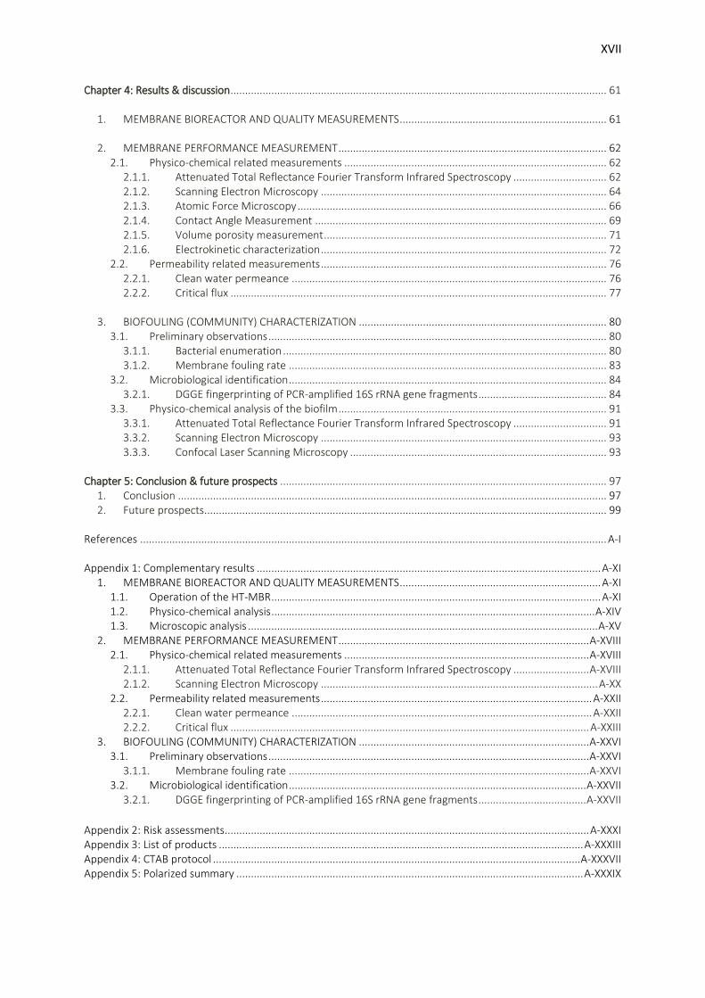
Chapter 4: Results & discussion ................................................................................................................................. 61

1. MEMBRANE BIOREACTOR AND QUALITY MEASUREMENTS ....................................................................... 61

2. MEMBRANE PERFORMANCE MEASUREMENT ............................................................................................ 62 2.1. Physico-chemical related measurements .......................................................................................... 62

2.1.1. Attenuated Total Reflectance Fourier Transform Infrared Spectroscopy ................................ 62 2.1.2. Scanning Electron Microscopy .................................................................................................. 64 2.1.3. Atomic Force Microscopy .......................................................................................................... 66 2.1.4. Contact Angle Measurement .................................................................................................... 69 2.1.5. Volume porosity measurement ................................................................................................. 71 2.1.6. Electrokinetic characterization .................................................................................................. 72

2.2. Permeability related measurements .................................................................................................. 76 2.2.1. Clean water permeance ............................................................................................................ 76 2.2.2. Critical flux ................................................................................................................................. 77

3. BIOFOULING (COMMUNITY) CHARACTERIZATION ..................................................................................... 80

3.1. Preliminary observations .................................................................................................................... 80 3.1.1. Bacterial enumeration ............................................................................................................... 80 3.1.2. Membrane fouling rate ............................................................................................................. 83

3.2. Microbiological identification ............................................................................................................. 84 3.2.1. DGGE fingerprinting of PCR-amplified 16S rRNA gene fragments ............................................ 84

3.3. Physico-chemical analysis of the biofilm ............................................................................................ 91 3.3.1. Attenuated Total Reflectance Fourier Transform Infrared Spectroscopy ................................ 91 3.3.2. Scanning Electron Microscopy .................................................................................................. 93 3.3.3. Confocal Laser Scanning Microscopy ........................................................................................ 93

Chapter 5: Conclusion & future prospects ................................................................................................................ 97

1. Conclusion ................................................................................................................................................... 97 2. Future prospects .......................................................................................................................................... 99

References ................................................................................................................................................................ A-I Appendix 1: Complementary results ...................................................................................................................... A-XI

1. MEMBRANE BIOREACTOR AND QUALITY MEASUREMENTS ..................................................................... A-XI 1.1. Operation of the HT-MBR ................................................................................................................. A-XI 1.2. Physico-chemical analysis ............................................................................................................... A-XIV 1.3. Microscopic analysis ........................................................................................................................ A-XV

2. MEMBRANE PERFORMANCE MEASUREMENT ...................................................................................... A-XVIII 2.1. Physico-chemical related measurements .................................................................................... A-XVIII

2.1.1. Attenuated Total Reflectance Fourier Transform Infrared Spectroscopy .......................... A-XVIII 2.1.2. Scanning Electron Microscopy ............................................................................................... A-XX

2.2. Permeability related measurements ............................................................................................. A-XXII 2.2.1. Clean water permeance ....................................................................................................... A-XXII 2.2.2. Critical flux ........................................................................................................................... A-XXIII

3. BIOFOULING (COMMUNITY) CHARACTERIZATION ............................................................................... A-XXVI 3.1. Preliminary observations .............................................................................................................. A-XXVI

3.1.1. Membrane fouling rate ....................................................................................................... A-XXVI 3.2. Microbiological identification ...................................................................................................... A-XXVII

3.2.1. DGGE fingerprinting of PCR-amplified 16S rRNA gene fragments ..................................... A-XXVII

Appendix 2: Risk assessments ............................................................................................................................. A-XXXI Appendix 3: List of products ............................................................................................................................. A-XXXIII Appendix 4: CTAB protocol .............................................................................................................................. A-XXXVII Appendix 5: Polarized summary ....................................................................................................................... A-XXXIX

Chapter 1: Context & objectives

1. BACKGROUND AND PROBLEM STATEMENT

The growth of world populations, the increasing industrialization and the expansion of intensive

agriculture from the 19th century pressurizes natural ecosystems in general and water bodies in

particular [1]. Increased water consumption combined with an alarming deterioration of the water

resource quality and the projections of climate change make water the most precious and important

common good worldwide. Thus sanitation technology for the treatment of wastewaters produced by

households or industrial activities is of strategic importance in order to provide the world populations

with sufficient amounts of fresh water in the future and to ensure environmental protection.

The currently most commonly used wastewater treatment technology is the Conventional Activated

Sludge Process (CASP), where pollutants and organics are removed from municipal and industrial

wastewaters by biological degradation and subsequent separation of the cleaned water by

sedimentation. Research aiming at improvement of this traditional approach started in the 1960s with

alternative membrane based treatment technologies, which improve the separation efficiency by

means of a filtration step through a membrane instead of sedimentation [2]–[6]. Driven by the

increasing water scarcity and the more stringent regulations, Japan, South Korea, France and the UK

have performed most of the pioneering research around membrane bioreactors (MBRs), so it’s not

surprising the first full-scale MBR plant for treatment of municipal wastewater has been installed in

the UK in 1997. Yet MBR technology can now be considered an established wastewater treatment

system delivering higher effluent quality as well as requiring a smaller footprint than the CASP [4].

The quantity and size of MBRs worldwide has increased exponentially with capacities ranging from < 1

m³ day-1 to > 100 000 m³ day-1 [7]. However, aside from the high investment cost, one of the main

drawbacks and research challenges of membrane technology is membrane fouling. Due to membrane

fouling the performance of the filtration process decreases with time, which implies high energy

demands and operational costs related to fouling prevention, mitigation and remediation. Example

studies on membrane fouling in view of process optimization are manifold, but there still exists a lack

of knowledge about the microorganisms taking part in the fouling process (i.e., biofouling) and their

specific relation to the membrane surface chemistry and to the wastewater environment, thus slowing

down the development of more targeted anti-(bio)fouling strategies.

2 |

2. RESEARCH OBJECTIVES AND RESEARCH APPROACH

The purpose of this study is to elucidate the relationship between the specific surface charge (neutral,

positive, negative) of polyacrylonitrile (PAN) membranes and the development and composition of the

microbial community in the biofouling layer developed during 40 days in a submerged laboratory-scale

aerobic membrane bioreactor (HT-MBR) operated on protamylasse feed.

The effect of membrane composition on biofilm community structure and diversity is assessed by

answering three questions:

Does the bacterial biofouling community differ from the sludge community at a certain time point,

i.e., are bacterial populations from the sludge specifically enriched within a biofilm?

Does the bacterial biofouling community change with time, i.e., do temporal variations in local

conditions favour or exclude specific bacterial populations?

Does the bacterial biofouling community on a membrane differ from the one on another

membrane type at a certain time point, i.e., does the membrane morphology, and more specifically

do the membrane surface charges affect the biofilm community composition?

Two approaches are applied:

Performance determination of the membranes based on physico-chemical related measurements

(ATR-FTIR, SEM, AFM, CAM, volume porosity measurement, electrokinetic characterization) and

permeability related measurements (CWP, critical flux);

Biofouling characterization based on molecular techniques (PCR-DGGE) and physico-chemical

techniques (ATR-FTIR, SEM, CLSM).

Chapter 2 of this work briefly explains conventional wastewater technology and reviews literature on

membrane technology and membrane fouling as to introduce the reader on the topic and on the

commonly used concepts and terminology. Chapter 3 presents the research plan comprising the

methodology and planning of the experiments. Finally Chapter 4 gives an interpretation of the results,

before concluding this work with some recommendations and future research perspectives.

| 3

Chapter 2: Literature review

1. CONVENTIONAL WASTEWATER TREATMENT

The wastewater treatment principles, including an overview of the chemical and biological

components of wastewater as well as a presentation of the conventional treatment train, are

highlighted as springboard towards the introduction to alternative wastewater treatment

technologies.

1.1. Wastewater treatment

1.1.1. Wastewater composition

Wastewater is defined as “domestic sewage or liquid industrial waste that cannot be discarded in

untreated form into lakes or streams due to public health, economic, environmental, and aesthetic

considerations” [8]. Roughly spoken, untreated wastewater is a complex mixture of natural or man-

made organic and inorganic compounds and potentially pathogenic microorganisms [1], [8], [9].

The composition of industrial wastewater varies according to the nature of the industrial process

generating it. For instance, while wastewaters originating from the food processing industry (e.g.,

dairy, meat, sugar) are rich in dissolved and suspended organics (proteins, fats, sugars), wastewaters

from the pharmaceutical or textile industry are enriched in surfactants and inorganic compounds [10].

On the contrary, municipal wastewater has a much more stable composition, but still depends on the

weather variability (i.e., dilution with rainwater) and the life styles and technologies practiced in the

producing society [1], [9]. The Flanders Environment Agency uses the ‘inhabitant equivalent’ to

designate the amount and composition of wastewater produced daily per Flemish inhabitant [11]. It

assumes an average Flemish wastewater composition of 90 g TS1, 54 g BOD2, 135 g COD3, 10 g TN4 and

2 g TP5 taking into account a daily wastewater flow of 150 l capita-1 [9], [11]. The removal of

1 The total solids (TS) (g l-1) represent the total amount of suspended and dissolved organic and inorganic solids in the sludge suspension [53].

2 The biological/biochemical oxygen demand (BOD) (g l-1) represents the relative amount of dissolved oxygen (mg O2 l-1) used by non-

photosynthetic microorganisms to catalyze the biodegradation of dissolved and particulate compounds present in the wastewater [8], [11]. 3 The chemical oxygen demand (COD) (g l-1) represents the amount of BOD together with the amount of organic compounds that are

chemically degradable. The COD does not comprise the oxygen necessary to oxidize nitrogen compounds but do comprise the oxygen needed to oxidize reduced sulfur compounds (SH-1, S2-) [11]. 4 Total nitrogen (TN) is a measure for the total amount of nitrogen compounds present in the wastewater, i.e., organic nitrogen (amino

acids) but also inorganic nitrogen (ammonium (NH3-N and NH4+-N), nitrite (NO2

--N) and nitrate (NO3--N)) [11].

5 Total phosphorus (TP) is a measure for the total amount of phosphate compounds present in the wastewater, i.e., organic phosphates (e.g.,

present in nucleic acids) but also inorganic phosphates (mainly orthophosphate PO43-) [11].

4 |

biodegradable substances (i.e., BOD), nitrogen and phosphorus species (NO3- -N, NO2

- -N, NH4

+ -N and

PO43- -P) is crucial as to avoid eutrophication of the receiving water bodies and toxicity to aquatic

organisms [1], [12]–[14]. Typical criteria for discharge of treated wastewater in surface waters

depends on the type of wastewater (domestic versus industrial) and on the producing industrial

sector, but are in the range of 30 mg TS l-1, 20 mg BOD l-1, 100 mg COD l-1, 10 mg TN l-1 and 1 mg TP l-1

[11], [12], [15].

1.1.2. Wastewater treatment train

Treatment of wastewater dates from the late 1800s [11] and has as primary goal to eliminate toxic

compounds and to reduce the amount of organic and inorganic compounds in the wastewater to a

level where microbial growth becomes limited [8]. Today the most commonly used wastewater

treatment technology for municipal and industrial sewage is a three-stage wastewater treatment

train, consisting of primary, secondary and tertiary treatment technologies (Figure 1) [4], [6]. Mainly

secondary or biological wastewater treatment has contributed largely to the improvement of the

quality of water bodies worldwide for almost a century [13], [16].

Figure 1 Schematic of a typical three-stage wastewater treatment train, comprising a primary treatment, secondary treatment or Conventional Activated Sludge Process (CASP) and a tertiary treatment, after which the

treated water is discharged in surface waters. The CASP detailed here, configured as the University of Cape Town (UCT-CASP) process, is the most commonly used configuration. VFA = volatile fatty acids.

(based on [9], [11], [12]).

1.2. Secondary wastewater treatment: CASP

1.2.1. Configuration: UCT-CASP

Different secondary wastewater treatment configurations exist aiming at the removal of the majority

of the soluble and suspended organic matter (carbon (C)) and mineral nutrients (nitrogen (N) and

| 5

phosphorus (P), e.g., NH4+ -N, NO3

- -N, PO43- -P) from the wastewater, but the most commonly used

Conventional Activated Sludge Process (CASP) for the treatment of wastewaters is the configuration of

the University of Cape Town (UCT-CASP) [17]. The UCT-CASP is a continuously operated system

consisting of a set of perfectly mixed basins connected by means of internal recirculation streams as

showed in detail in Figure 1. In principle the UCT-CASP process could be optimized by incorporating

multiple anoxic and aerobic zones in order to improve nutrient removal and lower energy costs [17].

Several microbially catalyzed reactions sequentially remove P, N and C compounds by conversion to

N2, CO2 and H2O and into a flocculent microbial suspension. P removal is typically achieved by the

activity of Phosphate Accumulating Organisms, such as Propionibacter and Acinetobacter, which

release PO43- -P in anaerobic conditions but take up a larger amount of inorganic phosphate from the

suspension under aerobic conditions. This results in a net accumulation of phosphate in their biomass

(cells can accumulate up to 24% of their dry mass in the form of phosphate) [11], [12], [17]. N removal

is typically based on a classical nitrification-denitrification process. The first step in N removal is

achieved based on nitrification reactions catalyzed by autotrophic organisms, e.g., Nitrosomonas,

Nitrosococcus and Nitrosospira on the one hand (NH3 NO2-) and e.g., Nitrobacter, Nitroeystis,

Nitrococcus, Nitrospora and Nitrospira on the other hand (NO2- NO3

-) under aerobic conditions

[11]–[14]. Finally heterotrophic micro-organisms complete the N removal by denitrification under

anoxic conditions (NO3- N2): Pseudomonas, but also Acinetobacter, Flavobacterium, Agrobacterium,

Chromobacterium, Achromobacter, Alcaligenes, Hyphomicrobium, Paracoccus, Thauera sp. and

Bacillus are reported to participate in the reactions [11]–[14]. Less energy-demanding novel nitrogen

removal processes are under investigation for implementation at large scale [11]: the SHARON6

process where the denitrification step starts from NO2- instead of NO3

- [18], [19]; the ANAMMOX7

process where NO2- and NH4

+ react together anaerobically to directly produce N2 [20], [21]; the

CANON8 process where NH4+ is converted to N2 in a single oxygen-limited step [22], [23]; or a

combination of these processes.

The series of perfectly mixed basins is followed by a secondary conventional gravity clarifier which

separates the purified water from the microbial biomass. The sedimentation efficiency depends on the

settling characteristics of the sludge, e.g., the size, shape and density of the particles, the composition

and concentration of the suspension, but also on the hydrodynamic conditions in the sedimentation

tank [9], [16]. The majority of the concentrated sludge is recirculated to ensure a high level of

biodegradation, while the excess sludge may be processed for energy recovery or disposal [11]. 6 Single reactor system for High Ammonia Removal Over Nitrite

7 ANaerobic AMMonium OXidation 8 Completely Autotrophic Nitrogen removal Over Nitrite

6 |

1.2.2. Sludge composition

The mixture of water and microbes in the perfectly mixed basins is called mixed liquor and consists of

suspended solids (i.e., microorganisms and inert material present as flocs typically at a size ranging

between 10 and 600 µm [24], [25]), dispersed microorganisms and organic and inorganic substances

[2], [4], [11], [26], [27].

The secondary clarifier receives the mixed liquor and separates the microbial biomass from the

purified water. Actually, the microbial biomass, also called activated sludge, is a diverse and

uncontrolled consortium of dead cells and interacting organisms (average ratio 50%-50%) [11]

including approximately 95% bacteria (cell length 1-5 µm [28]) and 5% higher organisms which are

mostly present free in the water phase, such as protozoa9, metazoans10 and fungi (cell length 10-10

000 µm [28]) (Figure 2) [5], [6], [11], [26], [29]. The dominance and balance of organisms present in

the activated sludge determines the overall health of the system [26]. For an extensive discussion on

the microorganisms and parameters affecting the activated sludge system, please refer to Eikelboom

(2000) [28].

Figure 2 Illustration of the evolution with time of the microorganism community in activated sludge (adapted from [30]).

Bacteria have the main role of removing the nutrients from the wastewater. Vanysacker et al. (2014)

report the number of bacteria present in activated sludge to reach 1013 bacteria ml-1 [16], which is

higher than in natural environments (typically 107 bacteria ml-1 in freshwater habitats [8]). Bacteria

living in activated sludge systems can be divided morphologically into floc-forming and filamentous

9 Protozoa, consisting of ciliates, flagellates and amoebas, are unicellular microorganisms [28]. They make up to 3% of the activated sludge

microorganisms and are considered to be the activated sludge cleaners by digestion of free-swimming bacteria and feeding on soluble organic nutrients [26].

10 Metazoans are multicellular microorganisms consisting of i.a., rotifers and nematodes. They have little impact on wastewater treatment

and mainly dominate old sludge [41].

| 7

bacteria [8]. The slow-growing filamentous bacteria are important for the development of well settled

sludge in the secondary clarifier. Indeed, they form the backbone network or macrostructure of flocs

by bridging behaviour [31], upon which a variety of small fast-growing floc-forming bacteria can

adhere (‘Filamentous Backbone Theory’) as well as soluble, colloidal and suspended organics [6]. An

excess of filamentous bacteria can cause sludge bulking in the clarifier and scum formation in the

aeration basin [26], [29].

Sludge bulking is generally caused by e.g., Sphaerotilus natans, Microthrix parvicella, Thiothrix spp,

Type 021N11, Type 0803/0914 or Haliscomenobacter hydrossis [28], [29], [32] and occurs when

approximately 107 µm ml-1 filaments are present in the activated sludge [11], [26]. Bulking sludge is a

sludge characterized by slow compaction and poor settling [29], resulting in large, open and irregular

floc structures due to excessive interfloc bridging [31].

Sludge foaming may be caused by fats or detergents present in the wastewater, but is more generally

caused by the hydrophobic filamentous bacteria Microthrix parvicella and to a limited extent,

Nostocoida limicola [28]. They produce high amounts of tensio-active biopolymers and induce scum

formation, which results in odour and aesthetic problems, extra cleaning work and potential damage

to the equipment [28].

1.3. Alternative technologies

The choice of wastewater treatment technology depends on physical and operational aspects, such as

the wastewater origin, the volumetric flow or the pollutant concentration, as well as the objectives

that have to be achieved (e.g., effluent standards) [9]. Although the CASP is the most widespread

method to treat both municipal and industrial wastewater and typically has a lifespan of minimum 20

years [9], it has a series of disadvantages, as will be highlighted further in this chapter, Section 2.3.2.

Therefore several authors have discussed alternative technologies to CASP.

1.3.1. Anaerobic digestion

Smets (2012) reported the combination of aerobic wastewater treatment followed by anaerobic

digestion of the produced excess sludge [11]. Hereby bacteria involved in anaerobic biodegradation of

organic material – a four-step process at high temperatures (20-75°C) [33] involving acidification and

methanogenesis – produce biogas, typically containing 70-90% CH4, 3-15% CO2 and 0-15% N2 gas [33].

The CH4 gas may be recycled for fuel production or combusted to produce electricity and heat,

generating approximately 380 kWh per 100 kg COD treated [5], [34], [35].

11 Most filamentous microorganisms do not have a name but a number [28].

8 |

1.3.2. Conventional anaerobic reactor

Liao et al. (2006) and Smets (2012) discussed the use of an anaerobic reactor as a wastewater

treatment technology on its own for the treatment of industrial (e.g., pulp & paper, textile,

pharmaceutical, chemical industry), agricultural and food processing wastewaters (e.g., beverage

industries) [11], [34]. These wastewaters typically contain large amounts of insoluble organic

compounds [8] and thus are characterized by high organic strengths12 (1000-85 000 mg COD l-1) [34].

For instance the Upward-flow Anaerobic Sludge Blanket Reactor (UASB) was discovered in the 1970s

and consists of a sludge bed composed of microorganisms that form granules or pellets of 1-3 mm

diameter. These pellets have sedimentation velocities up to 100 m h-1 and are not washed out, in

contrast to flocs. Table 6 compares the characteristics of the UASB to the CASP. Anaerobic systems

tend to achieve an effluent quality that is lower than in CASP due to the slow growth rates of the

microorganisms. Anaerobic systems thus are mainly exclusively used for concentrated waste streams,

while the CASP is used for more diluted waste streams (e.g., municipal water characterized by an

organic strength between 250-800 mg COD l-1 and suspended solids concentration between 120 and

400 mg l-1) [34]. Liao et al. (2006) reported the presence of almost 1600 anaerobic wastewater

systems worldwide [34].

1.3.3. Membrane bioreactor

The most recent advances in wastewater treatment technology reside in the development of

membrane bioreactors (MBRs). The pollutants from the wastewater undergo the same treatment as in

the CASP but the sedimentation in the final clarifier is replaced by filtration through a membrane [11],

[14]. For several years researchers have taken a closer look at both aerobic and anaerobic MBRs and

their implementation in wastewater treatment. Next section gives a description of MBRs and their

field of application.

2. MEMBRANE BIOREACTOR FUNDAMENTALS

Membrane bioreactor technology is presented starting from a general definition and focus on the

main concepts and characteristics of membrane technology as core technology [2], including

membrane synthesis, module configuration and operating parameters. Finally current research trends

in the field are highlighted.

2.1. Definition

A MBR process is defined as the combination of two physical processes that aim at improving

wastewater treatment efficiency: a biological treatment by suspended biomass, similar to the CASP, is

12

The volumetric or organic loading rate (Bv) (kg COD m-³ d-1) represents the amount of substrate given daily to the microorganisms, expressed per reactor volume [11].

| 9

followed by liquid/solid separation by a porous membrane. Hereby the filtration through the

membrane replaces the gravity sedimentation to clear the wastewater effluent [2]–[6].

2.2. Membrane technology

2.2.1. Process classification

A membrane process is a continuous unit operation consisting of a filter (porous or semi-permeable

membrane) between two phases, the concentrated retentate, and the purified permeate (Figure 3).

The membrane allows selective migration of compounds present in the influent depending on their

size, shape and charge [36]. Migration through the membrane is the result of the presence of a driving

force, either a temperature, pressure, concentration or electrical potential difference between the

retentate and permeate side of the membrane [38]. Here only pressure driven membrane processes

between two liquid phases are considered: a suction force is applied at the permeate side as to create

a small vacuum, which adds to the static pressure of the water, resulting in migration through the

membrane [36].

Figure 3 Schematic of a membrane process (adapted from [38]).

Four types of pressure driven membrane processes can be distinguished based on the properties of

the membrane (mainly pore size), the size and chemical properties of the particles or molecules

retained by the membrane, and the pressure applied [36]. An overview of these four types of

processes is given in Table 1.

Microfiltration (MF) and ultrafiltration (UF) membranes are mainly implemented in traditional

wastewater treatment plants. In general UF membranes result in better water quality and less

obstruction of the pores since they are less accessible for particles [5], [36], [39]. Nanofiltration (NF)

and reverse osmosis (RO) membranes have pores that may be hard to detect, called voids or free

volume [16]. Migration through RO membranes can result in retention from 80% to 99%, depending

on the specific compound [36]. The required effluent quality and the investment, treatment and

replacement costs are intimately dependent of the choice of process type [36].

10 |

Table 1 Properties of the four pressure driven membrane processes (adapted from [36]–[38], [40]–[43]).

Membrane process

13

Property Microfiltration Ultrafiltration Nanofiltration Reverse osmosis

Pore size (nm) 50-10 000 1-100 0.1-5 0.05-1

Applied pressure (bar) 0.2-2 1-10 10-20 20-100

Permeability

(l h-1

m-² bar

-1)

>> 50 10-50 1.5-15 0.05-1.5

Main separation principle Sieving Sieving

Sieving, diffusion/size

exclusion, charge

interactions

Diffusion/size exclusion

Membrane materials

most frequently used

Polymeric: e.g., PC14

, PEEK15

, PA16

,

P(E)I17

, P(E)S18

, cellulose esters, PP19

,

PE20

, PVDF21

, PTFE22

,

Inorganic: e.g., Al2O3, ZrO2, TiO2, SiC,

SiO2, stainless steel

Polymeric: e.g., PAN23

,

PVDF, PEEK, PA, P(E)I,

PES, cellulose esters

Inorganic: e.g., Al2O3,

ZrO2

Polymeric: e.g., cellulose

esters, PES, P(E)I, PA Polymeric : e.g., cellulose esters, PA

Most important

applications

Wastewater treatment, food industry,

metallurgy

Wastewater treatment, food

industry Food industry

Drinking water production, water

desalination, wastewater treatment

Retained compounds Suspended particles (fungi, bacteria,

colloidal solids, oil emulsions) Viruses

Macromolecules (proteins,

polysaccharides)

Antibiotics, pesticides, small organic

monomers (e.g., small sugars,

vitamins), inorganic ions (e.g. Na+,

K+, Cl

-, Ca

2+, Mg

2+, SO4

2-)

13

No sharp boundaries exist between membrane processes, so values for pore size, applied pressure and permeability indicated in Table 1 are guidelines rather than fixed values. 14

Polycarbonate, a hydrophilic polymer. 15

Polyetheretherketon, a hydrophilic polymer. 16

Polyamide, a hydrophilic polymer 17

Poly(ether)imide, a hydrophilic polymer. 18

Poly(ether)sulfone, a hydrophilic polymer. 19

Polypropylene, a hydrophobic polymer. 20

Polyethylene, a hydrophobic polymer. 21

Poly(vinylidene fluoride), a hydrophobic polymer. 22

Polytetrafluoroethylene, a hydrophobic polymer. 23

Polyacrylonitrile, a hydrophilic polymer.

| 11

2.2.2. Membrane morphology and membrane materials

Membranes are classified according to their morphology: symmetric membranes are distinguished

from asymmetric membranes (Figure 4). Both are either porous or dense, but while the former

exhibits the same structure along its cross-section, the latter does not and may even consist of several

layers which can be optimized independently. These are so-called composite membranes. Symmetric

membranes are self-supporting and have a working thickness of 10-200 µm. In asymmetric

membranes, it is the 0.1-0.5 µm selective active skin layer that determines the flux, resistance and

rejection characteristics. This skin layer is physically supported by a 50-150 µm porous substructure

[37], [38], [44].

Figure 4 Classification of membranes based on their morphology (adapted from [38]).

While membrane morphology determines the efficiency of the membrane, membrane material

determines the structural (thermal, chemical and mechanical) properties of the membrane [38]. In

general membranes must exhibit a high permeability and selectivity, combined with sufficient

chemical, thermal and mechanical stability [36].

Organic membranes are distinguished from inorganic membranes (Table 1). In pressure driven

processes on aqueous systems, most membranes are constructed from organic or polymeric materials

[45]. On the contrary, inorganic membranes may be applied for the purification of strongly alkaline or

acid mixtures as well as in high temperature wastewaters. Some authors mention ceramic or metallic

materials (e.g., [46], [47]). Inorganic membranes are generally hydraulically, thermally and chemically

more stable than polymeric membranes, have a longer lifetime, are more fouling-resistant and their

pore size can be better controlled to maintain high fluxes. However, their use is limited in large-scale

applications since they are expensive and difficult to prepare [4], [36]–[38], [48]. Research is being

performed in order to develop new membrane materials which are cost-attractive and highly efficient

[48].

12 |

2.2.3. Membrane synthesis

As seen above, a lot of different membrane structures and materials exist, thus resulting in a large

number of membrane synthesis methods. The majority of the commercially available membranes are

polymeric and 90% of these are synthesized by the phase inversion process [38].

Phase inversion is a rapid process where a thermodynamically stable solution of a polymer and a

solvent (‘casting solution’) is transformed from a liquid to a solid asymmetric membrane by controlled

demixing by immersion in a coagulation bath containing a non-solvent. On the one hand, a continuous

polymer-rich phase is formed that will become the membrane matrix of the solid porous membrane.

On the other hand the open pore structure is obtained via the discrete polymer-lean phase [38].

2.2.4. Membrane modules

Membranes are generally mounted in separation units called modules, which are joined to form one

large filtration unit, called a process train (Figure 5) [49].

Figure 5 MBR membrane configurations: membrane, module and process train. (A) flat sheet, (B) hollow fibre, (C) multi-tubes (adapted from [4], [49]).

Depending on the type of separation to achieve, the maintenance requirements, the scale of the

system and the costs, different module designs are on the market with their own application area

(Table 2) [36], [38]. Based on geometry, modules made from flat-sheet membranes are distinguished

from modules made from a large number of tube-like membranes (tubular, capillary or hollow fibre

modules). Flat sheets are stacked either in vertically plate-and-frame modules or in spiral-wound

modules. Both consist of two membrane sheets separated by an internal spacer, but in the latter

configuration the system is wrapped around a central collection pipe and placed in a pressure tube.

The spacer layer is a turbulence promoter aiming at reducing the risk of fouling [36], [38]. For a

discussion on the appropriateness of flat sheet membranes versus tube-like membranes, please refer

to Gunder et al. (1998) and Judd (2002) [50], [51].

| 13

Table 2 Comparison of the modules design and their characteristics (adapted from [5], [36], [38]).

Module design

Characteristic Tubular

(ϕ > 10 mm)

Plate and

frame

Spiral

wound

Capillary

(0.5 < ϕ < 10 mm)

Hollow fibre

(0.5 mm > ϕ)

Packing density Low (150-300

m² m-3

)

High (200-500 m²

m-3

)

Investment high low

Fouling tendency Low Very high

Cleaning efficiency Good Poor

Membrane

replacement Yes/no Yes No No No

Application

MF, UF

In-to-out

filtration

MF, UF MF, UF,

(NF, RO)

MF, UF

In-to-out filtration

NF, RO, (MF, UF)

Out-to-in filtration

2.2.5. System design

In pressure driven membrane processes, the separation can be obtained in two ways: either by dead-

end filtration, or by cross-flow filtration (Figure 6) [36]–[38]. During dead-end filtration the feed

solution is applied perpendicular to the membrane surface. During cross-flow filtration the feed and

permeate solution flow along the membrane, parallel with the surface in co-current or counter-

current directions. Although dead-end filtration is energetically advantageous since it requires less

pumping energy for filtration thanks to the hydraulic pressure built-up, the majority of the industrial

applications is based on cross- flow filtration mode [36]. The main reason is the occurrence of fouling,

whereby regularly cleaning of the membrane becomes necessary.

Figure 6 Dead-end filtration (A) versus cross-flow filtration (B) (adapted from [37]).

2.2.6. Operating parameters

Volumetric flux and transmembrane pressure

According to Wang et al. (2009) the simplest model to describe ideal transport of liquids through a

porous membrane is by considering a membrane as a number of uniformly distributed and evenly

sized parallel cylindrical pores which cover the full membrane cross-section [45]. The volume flux may

be described by the Hagen-Poiseuille equation:

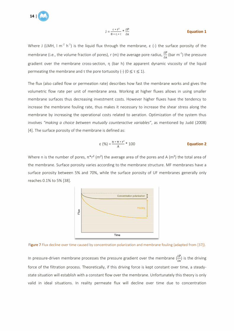
14 |

J =

*

Equation 1

Where J (LMH, l m-2 h-1) is the liquid flux through the membrane, (-) the surface porosity of the

membrane (i.e., the volume fraction of pores), r (m) the average pore radius,

(bar m-1) the pressure

gradient over the membrane cross-section, (bar h) the apparent dynamic viscosity of the liquid

permeating the membrane and the pore tortuosity (-) (0 1).

The flux (also called flow or permeation rate) describes how fast the membrane works and gives the

volumetric flow rate per unit of membrane area. Working at higher fluxes allows in using smaller

membrane surfaces thus decreasing investment costs. However higher fluxes have the tendency to

increase the membrane fouling rate, thus makes it necessary to increase the shear stress along the

membrane by increasing the operational costs related to aeration. Optimization of the system thus

involves “making a choice between mutually counteractive variables”, as mentioned by Judd (2008)

[4]. The surface porosity of the membrane is defined as:

(%) =

* 100 Equation 2

Where n is the number of pores, π*r (m ) the average area of the pores and A (m ) the total area of

the membrane. Surface porosity varies according to the membrane structure. MF membranes have a

surface porosity between 5% and 70%, while the surface porosity of UF membranes generally only

reaches 0.1% to 5% [38].

Figure 7 Flux decline over time caused by concentration polarization and membrane fouling (adapted from [37]).

In pressure-driven membrane processes the pressure gradient over the membrane (

) is the driving

force of the filtration process. Theoretically, if this driving force is kept constant over time, a steady-

state situation will establish with a constant flow over the membrane. Unfortunately this theory is only

valid in ideal situations. In reality permeate flux will decline over time due to concentration

| 15

polarization24 or fouling (Figure 7) [38], a phenomenon that will be explained in next section. The

pressure difference over both permeate (Ppermeate) and retentate side (Pretentate) of the membrane, P, is

called the transmembrane pressure (TMP) [40], [52]:

P = Pretentate – Ppermeate Equation 3

Both the flux and TMP define the operating range of the MBR process [40].

Permeability coefficient

Apart from the flux-concept described above, the efficiency of a membrane process can be expressed

by several other parameters. One of these parameters is the permeability coefficient (l m-1 h-1 bar-1),

P’, which is an intrinsic property of the membrane material and mainly affected by the operating

temperature and the particle size distribution of the mixed liquor [40], [53]. It is defined as the

permeance (LMH bar-1), K, multiplied by the membrane thickness, x, or also as the flux per unit TMP

multiplied by the membrane thickness [4], [38]:

P’ = K * x =

* x Equation 4

2.2.7. Critical flux concept

As already mentioned above, one of the major problems in pressure-driven membrane processes is

the gradual reduction of the permeate flux below the theoretical capacity of the membrane during the

filtration process, due to fouling. Field et al. (1995) introduced the concept of critical flux (Jc) as

quantitative parameter for the assessment of cross-flow MF membrane performance, which may

enable identification of the appropriate operating conditions and optimization of the filtration process

[54], [55].

A filtration process can be conducted in two ways, either constant-flux or constant-pressure filtration.

The former involves the gradual increase in TMP in order to overcome the flux decline due to fouling

phenomena [56]. The latter involves the gradual decrease in flux while keeping the TMP constant.

Field et al. (1995) developed the hypothesis that on start-up of the filtration process, there exists a

flux below which a decline of permeate flux with time does (almost) not occur, while above that flux

fouling cannot be neglected and regularly cleaning becomes necessary [54]. This critical flux concept

involves that it may be possible to operate a constant-flux filtration during up to one month [56]

24

Concentration polarization is an increase of the concentration of retained substances near the membrane surface (from where water is selectively removed). It is inherent of membrane filtration but may induce membrane fouling. It can be decreased for instance by increasing turbulence in the mixed liquor [38].

16 |

without the obligation to gradually increase the TMP (i.e., operating at a sub-critical flux is

theoretically characterized by a membrane fouling rate d P/dt = 0 or a ratio dJ/d P = 0). However this

is almost never achieved. Even at low flux, marginal fouling does occur – mainly due to adsorption

phenomena [57], [58] – and TMP values must be slightly increased in order to maintain a constant flux

[56], [59]. When filtration progresses in long-term operations, more severe fouling becomes

unavoidable leading to a roughly exponential TMP increase above the critical TMP value and flux

decline [54], [59]. However van der Marel et al. (2009) reported that it is possible to operate at a flux

higher than the critical flux, as long as no significant irreversible fouling occurs, i.e., at a flux between

the critical flux and a flux of 100 l m-2 h-1 [60].

The estimated critical flux value and fouling rate on the short-term also depends on the methodology

used to assess it. The most widely used methodology is the TMP measurement in flux-stepping

experiments during constant-flux filtration. However the short-term flux-stepping methodology used

in laboratory- or pilot scale systems cannot be used to assess the long term fouling behaviour, nor in

laboratory- or pilot scale systems, nor in full-scale systems [48], [61].

2.3. Membrane bioreactor technology

2.3.1. Historical market development

Yang et al. (2006) performed an extended study around the evolution and implementation of MBR

technology in North-America [62], while Lesjean et al. (2008) surveyed the European MBR market

[63]. Research on membrane bioreactors (MBRs) started in the 1960s. MBR technology is now

implemented as ‘Best Available Technology' for the treatment of industrial wastewaters from e.g., the

food, pharmaceutical, textile or meet industry, which produce wastewaters with much more varying

composition and organic loading than municipal wastewater. GE-Zenon Environmental Inc. (Canada),

USFilter (USA), Kubota (Japan) and Mitsubishi-Rayon (Japan) are some of the largest European

membrane suppliers, but are gradually expanding towards emerging economies such as Brazil or China

[5]. It is expected that the technology will further develop as to respond to national and international

environmental, economic and political expectations [3], [64]. Frost & Sullivan (2013), as cited by Royan

(2014), estimated the global MBR market volume to be $ 838.2 million in 2011 (i.e., € 716.2 million

based on the actual conversion ratios) and is expected to increase up to $ 3.44 billion by 2018 (i.e., €

2.63 billion) [65], [66].

2.3.2. Prospects and constraints of the MBR technology

Several characteristics of MBRs make them advantageous compared to the CASP. However, many

barriers still limit the faster and larger development of this technology, as depicted in Table 3 and

Table 4 [5].

| 17

The most cited limitation of membrane filtration is membrane fouling. This phenomenon is related to

interactions between the membrane surface and the soluble and particulate matter present in the

activated sludge mixed liquor [16]. It mainly occurs in MF and UF filtration processes and is partly

responsible for the retardation of faster commercialization of MBR technology since it has a large

negative influence on the economics [38], [62], [67]. Membrane fouling is extensively discussed

further in this chapter, Section 3.

2.3.3. Process configurations

At the beginning of MBR technology development, the majority of MBRs were based on a side-stream

or external configuration (eMBR), where the membrane modules are located outside the reactor

(Figure 8) [40]. In 1989 an internal or immersed MBR (iMBR) was used for the first time for the

investigation of stable flux conditions and nutrient removal through hollow fibre membranes [68]. In

this configuration the membrane module is immersed in the basin containing the active sludge. iMBRs

now dominate the market [42]. Table 5 compares iMBRs and eMBRs.

Figure 8 Internal or immersed MBR (A) versus side stream or external configuration (B) (adapted from [4], [16], [40], [69]).

2.4. Current research trends

2.4.1. Anaerobic membrane bioreactors

One of the most widely explored trends in the last 10 years involves the development of immersed

and external anaerobic membrane bioreactors (AnMBRs). This technology combines the membrane

technology with anaerobic biological treatment (Figure 9) [4]. Actually, research around AnMBRs

started in the late 1970s but the technology could only be successfully implemented at large scale in

the 1990s [33], [34]. Nevertheless the process design still needs to be optimized further technically

and economically in order to ensure greater large scale utilization of AnMBRs. Lin et al. (2013), Liao et

al. (2006) and Stuckey (2012) reviewed extensively recent literature about AnMBRs [33], [34], [42]. For

instance they reviewed the application of AnMBRs with different kinds of wastewater (synthetic,

industrial, food processing, municipal) and at different scales (laboratory, pilot, full scale). They

concluded that the AnMBR technology is mainly applicable to highly concentrated/high strength and

particulate/high solids wastewater, such as sludge and wastewater from slaughterhouses.

18 |

Table 3 Advantages of the MBR technology compared to the CASP.

Advantage compared to CASP Additional notes References

Space requirement and

environmental footprint

Compact because of the absence of settling requirements which limits the sludge concentration to 5 g l-1

and imposes large basins, thus applicable in space-limited locations. For instance, compare an average

surface of 4452 m² (CASP) to 190 m² (MBR) for the treatment of 100 000 kg COD day-1

.

[4]–[6], [11], [16], [24],

[25], [35], [36], [40], [56],

[67], [69]–[74]

Easy up-scaling Modular and compact design. Possible to assess technical and economical feasibility on a small-scale.

Moreover possible to integrate in existing CASP. [36]–[38], [48], [69]

Higher and constant effluent

quality

The filtered effluent is nearly free of particles, bacteria and soluble organic substances, while in theory

an infinite settling time is necessary in the CASP to obtain the same result. For instance, the presence of

coliform bacteria25

may be reduced to a factor log 7 in the effluent compared to the original wastewater.

Moreover e.g., bulking sludge or foaming phenomena (Section 1.2.2) do not affect the liquid-solid

separation.

[3]–[6], [11], [16], [24],

[25], [36], [40], [64], [67],

[69]–[73], [75], [76]

Adjustable membrane properties Membranes can be optimized independently from each other and from the reactor process, for instance

in order to be compatible with the type of wastewater. [6], [36]–[38]

Decoupling of hydraulic (HRT26

)

and sludge retention time (SRT27

)

HRT can be reduced to a minimum (4-6 h) independent of SRT, which can be increased (up to 30 days),

thus offering great process control and increasing biomass concentration in the reactor.

[4]–[6], [25], [40], [71],

[73]

Less excess sludge

Excess sludge, which needs to be processed (drying, handling, incineration), is minimized thus reducing

overall costs. Moreover the produced excess sludge is more concentrated, thus making faster conversion

of biodegradable material possible and easier post-treatment.

[4]–[6], [9], [11], [16], [24],

[25], [35], [36], [56], [64],

[67], [70]–[74], [76]

25

Coliform bacteria are widely used as indicators for microbial water contamination [8] 26

The hydraulic retention time (HRT) (h) represents the average time the microorganisms have been in contact with the biodegradable compounds in the wastewater [11]. 27

The sludge residence time (SRT) (d) represents the average time the microorganisms reside in the reactor. The more often sludge is removed from the reactor, the smaller the SRT [11].

| 19

Table 4 Disadvantages of the MBR technology.

Disadvantages of the MBR Additional notes References

Flux decline (during constant-pressure

filtration) or increase in TMP over time

(during constant-flux filtration)

May be attributed to concentration polarization or fouling phenomena. [5], [11], [16], [25], [36],

[67], [69], [70], [76], [77]

High operational and maintenance

costs

Costs related to wastewater pretreatment, membrane cleaning, membrane/module replacement

and energy consumption (aeration, pumping). The latter reaches 0.2-1.5 kWh m-3

produced water

with a feed of 1 g COD l-1

). Membranes generally have a lifetime ranging from 3 to 8 years,

depending on the membrane type, the operating conditions, the cleaning frequency and the

characteristics of the influent.

[4], [5], [24], [36]–[38],

[42], [69], [71], [75]

Complex design and operation

Operational protocols need to be executed well in order to assure a long lifetime of the system.

Moreover MBR suppliers and users often lack knowledge about sludge properties and long-term

performances of the system since it is a relatively new technology.

[4], [5], [70]

Aeration and oxygen transfer

Lower oxygen transfer due to i.a., higher biomass concentration. Thus a more intensive aeration is

necessary in order to maintain a fast conversion of biodegradable material. On the other hand also

floc size does influence oxygen transfer. Flocs in MBRs experience shear rates and on average tend

to be 10 times smaller than flocs in CASP, resulting in higher oxygen transfer rates and removal

rates.

[4], [5], [16], [24], [36],

[69]

Variable investment costs

10-20% higher investment costs: large membrane surface area needed to maintain acceptable

overall flux.

Lower investment costs: no clarifier needed and compact installation. Moreover the cost of

membrane modules decreases with the years.

[4], [5], [36], [71]

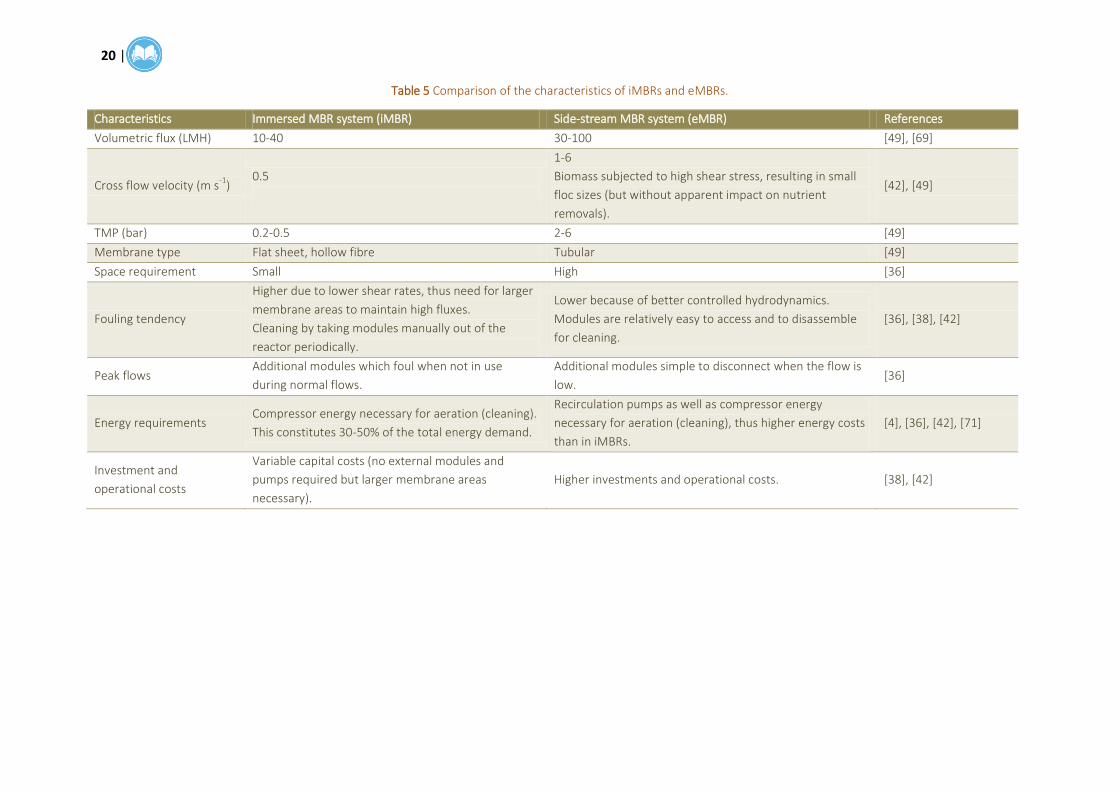
20 |

Table 5 Comparison of the characteristics of iMBRs and eMBRs.

Characteristics Immersed MBR system (iMBR) Side-stream MBR system (eMBR) References

Volumetric flux (LMH) 10-40 30-100 [49], [69]

Cross flow velocity (m s-1

) 0.5

1-6

Biomass subjected to high shear stress, resulting in small

floc sizes (but without apparent impact on nutrient

removals).

[42], [49]

TMP (bar) 0.2-0.5 2-6 [49]

Membrane type Flat sheet, hollow fibre Tubular [49]

Space requirement Small High [36]

Fouling tendency

Higher due to lower shear rates, thus need for larger

membrane areas to maintain high fluxes.

Cleaning by taking modules manually out of the

reactor periodically.

Lower because of better controlled hydrodynamics.

Modules are relatively easy to access and to disassemble

for cleaning.

[36], [38], [42]

Peak flows Additional modules which foul when not in use

during normal flows.

Additional modules simple to disconnect when the flow is

low. [36]

Energy requirements Compressor energy necessary for aeration (cleaning).

This constitutes 30-50% of the total energy demand.

Recirculation pumps as well as compressor energy

necessary for aeration (cleaning), thus higher energy costs

than in iMBRs.

[4], [36], [42], [71]

Investment and

operational costs

Variable capital costs (no external modules and

pumps required but larger membrane areas

necessary).

Higher investments and operational costs. [38], [42]

| 21

Figure 9 Anaerobic membrane bioreactor in immersed configuration (based on [11]).

Table 6 compares aerobic and anaerobic conventional and membrane systems. The effect of lots of

parameters on AnMBRs has been assessed recently but by using aerobic MBRs instead of AnMBRs and

simply assuming to be similar thus extrapolated to AnMBRs [4], [42]. For instance, a large amount of

work has been done concerning fouling in aerobic MBRs, as will be discussed later, but rather few

information is available about anaerobic fouling and the best ways to control it [5]. However it is

estimated that fouling control strategies in AnMBR are cheaper than in aerobic MBRs (0.80 kWh m-3

treated water with a feed of 1 g COD l-1 compared to around 2 kWh m-3 treated water for the same

feed) [42].

Table 6 Comparison of aerobic and anaerobic conventional and membrane systems

for the treatment of municipal wastewater (table based on [33] but extended with data from [4], [5], [34]–[36], [42], [43], [52], [56], [69]).

Parameter CASP UASB Aerobic MBR Anaerobic MBR

Start-up time 2-4 weeks 2-4 months <1 week <2 weeks

HRT (hour) 4-8 6-14 4-9 3-17

SRT (day) 3-15 30-100 5-20 >100

MLSS in bioreactor (g l-1

) 1-5 15-30 5-20 10-40

COD removal (%) <95 95-99 94-98

Effluent COD (mg l-1

) 30-70 100-220 10-30 <100

Effluent TSS (mg l-1

) <30 (5-8) 30-70 <1 <1

Effluent TN (mg l-1

) 8 5

Effluent PO43-

–P (mg l-1

) 1-3 0.3-3

Organic loading rate

(kg COD m-3

day-1

) <2 <30 <10 10-25

Anaerobic systems must be operated at higher temperatures than aerobic systems, thus consuming

more electricity (compare on average 0.45 kWh m-3 for an aerobic MBR versus 0.60 kWh m-3 for an

anaerobic MBR) [34]. This disadvantage could be balanced completely by recovery of the methane gas

as explained previously in this chapter (Section 1.3.1) [33]. Moreover Stuckey (2012) reviewed recent

literature demonstrating that anaerobic bioreactors could be operated stably at temperatures down

22 |

to 13°C [42]. However methane yield is strongly dependent on temperature, since methane is

approximately 1.5 times more soluble at 15°C compared to 35°C, thus rendering methane recovery

more difficult for lower temperature effluents [33]. Finally, although nutrient (N, P) removal in

AnMBRs is limited compared to aerobic systems, this can be seen as an opportunity to recover and

recycle these nutrients from the effluent of an AnMBR in view of reuse in agriculture [42].

2.4.2. Alternative membranes

Another current research topic involves the development of alternative membranes including low-cost

filters, dynamic membranes and membrane modifications [78], mainly in order to decrease the

investment and operational costs of MBRs. Low-cost filters encompass non-wovens, meshes and filter

cloths and may be used in applications that do not require high end-product quality [48]. Precoated or

self-forming dynamic membranes are synthesized by filtering a solution of one or more membrane-

forming materials such as hydrated oxides, polymers or colloidal materials through a porous support.

This dynamic forming method is mainly used for the synthesis of NF and RO membranes [79]. Finally

membrane surface modifications are mainly applied in order to increase the hydrophilic character of a

hydrophobic membrane in order to limit its fouling tendency [78]. For an extensive review of these

topics, please refer to Meng et al. (2009) [48].

2.4.3. Alternative configurations

Li et al. (2005) studied the development of Aerobic Granular-Sludge Membrane Bioreactors which

would be more effective for fouling control than normal aerobic MBRs [80]. These reactors contain

large sized, dense, granular sludge as substitute for sludge flocs.

Finally research is being performed around extractive and diffusive MBRs in view of future

commercialization [4], [52]. In ‘normal’ MBRs, the biomass is retained by the membrane while the

permeate goes through it. In contrast, in diffusive MBRs the membrane is used to introduce a gas in its

molecular form directly into the biofilm on the membrane surface in the bioreactor. This gas is then

used for biotreatment. In extractive MBRs the membrane is used to extract specific (toxic) compounds

from the reactor across the membrane in order to treat them biologically.

3. FUNDAMENTALS OF MEMBRANE FOULING

Figure 10 emphasizes the growing importance of fouling in MBR filtration processes. Membrane

fouling is one of the major problems concerning membrane filtration processes to be resolved, but

because of the complexity of the fouling mechanisms and the variety of parameters influencing it, it is

still unclear how to respond efficiently to that problem [16]. Moreover different researchers all

| 23

implement different operating conditions and module configurations during their investigations, thus

making it difficult to draw uniform conclusions. For an intensive review on membrane fouling and

fouling control actions, please refer to Wang et al. (2014) [81].

Figure 10 Evolution of the annual publications on MBR fouling, searched via Google Scholar until 2008 and via PubMed from 2009 to 2014 (adapted from [48]).

3.1. Definition

Judd (2008) defined fouling as “the restriction, occlusion or blocking of membrane pores at the surface

of the membrane, reducing the flow of permeate water through the membrane material” [4].

Membrane fouling is provoked by undesirable deposition and accumulation of salts, macromolecules,

microorganisms, colloids, solutes and cell debris onto or within the membranes [75].

3.2. Classification of membrane fouling

Membrane fouling can be classified in three ways:

based on the mechanism;

based on the permeability recovery;

based on the nature of the foulants.

3.2.1. Classification based on the mechanism

Grelier et al. (2006) defined the fouling rate d P/dt as “the gradient of membrane resistance over

time” [2] which can be written as [38], [52]:

Rt = Rm + Rf Equation 5

Where Rt (m

-1) is the total membrane resistance, Rm (m-1) is the intrinsic clean or hydraulic resistance

of the membrane and Rf (m-1) is the time-dependent resistance due to fouling and concentration

polarization (Rcp). Rm is independent of mixed liquor characteristics or applied pressure and indicates

the tolerance of the membrane against hydraulic pressure [78].

24 |

Ye et al. (2005) and Liang et al. (2005) defined the flux using the TMP and the concept of resistance

(‘Resistance-in-series model’) [55], [71]:

J =

=

Equation 6

With (Pa h) the viscosity of the feed solution. Rf can be further divided into resistance due to surface,

external or macro-fouling and resistance due to pore, internal or micro-fouling (Figure 11) [24], [40].

Rf = Rg + Rp + Ra + Rcp Equation 7

The former includes resistance due to deposition and accumulation of particles on the membrane

surface, eventually leading to a gel or cake layer (Rg) (Figure 11). Cake layer formation is caused by

particles with a size larger than the membrane pore size [49]. The cake layer is a porous structure on

top of the membrane [48] that resembles the composition of the biomass flocs [82]. Lee et al. (2001)

assumed the cake layer to contribute up to 80% to total membrane resistance [83].

Figure 11 Membrane fouling mechanisms. (A) surface fouling, (B) pore fouling, (C) cake layer formation (adapted from [38]).

Pore or micro-fouling includes resistance due to pore blocking via soluble organic or microbiological

material (Rp) or resistance due to partial pore closure by adsorption of solutes or colloids on the walls

on the pore channels (Ra). Pore blocking is caused mainly by particles with a size comparable to the

membrane pore size, while pore closure is caused by particles that are smaller than the pores [49].

3.2.2. Classification based on the permeability recovery

Ye et al. (2005) and Liang et al. (2005) wrote Rf in terms of the degree of fouling removability [55],

[71]:

Rf = Rirrev + Rr + Rirrec Equation 8

Rirrev (m-1) is the irreversible or permanent fouling mainly caused by pore blocking by dissolved organic

substances [71], [84] and is believed to be independent of filtration time [58]. Irreversible fouling is

often insignificant compared to Rt or Rf [58] and can only be reduced to zero by using chemical

cleaning methods [71].

| 25

Rr (m-1) is the removable, reversible or temporary fouling and also includes the concentration

polarization. Rr is mainly attributed to cake layer formation by mixed liquor suspended solids (MLSS)

[48], [71] and can be removed by hydraulic cleaning methods [4], [71], [84].

Finally Judd (2008) also defined long-term irrecoverable, irremovable or absolute fouling, Rirrec (m

-1)

[4], which cannot be removed by any cleaning method and which defines membrane lifetime [48].

However, these three types of fouling are often defined differently in literature, often due to

differences in measurement protocols, resulting in confusing situations where the meaning of the

terms irreversible and irremovable fouling is interchanged [16], [48].

3.2.3. Classification based on the nature of the foulants

Recent reports [6], [16], [38], [48], [85] distinguished three types of foulants occurring simultaneously,

based on their physical and chemical characteristics: organic precipitates, inorganic precipitates and

biofouling.

Organic and inorganic precipitates

Organic precipitates are deposited biopolymers (proteins and carbohydrates) or humic substances

(dissolved organic matter) resulting from non-covalent interactions between macromolecules or

complexation reactions involving metal ions (e.g., Ca2+, Mg2+) present in the feed solution and the

mixed liquor [25], [76], [86].

Inorganic precipitates are inorganic salts (e.g., CaSO4, CaCO3, SiO2, Fe(OH)3) present in the feed

solution and the mixed liquor that precipitate (‘scaling’) onto the membrane surface due to

concentration polarization or pH and temperature variations [85], [87].

Biofouling and biofilm formation

Biofouling refers to the undesirable gradual attachment on the wet membrane surface of individual

cells, cell clusters or materials of biological origin present in the mixed liquor [88]. The bacteria

present in the biofilm are believed to depend on the composition of the bulk solution, although it has

been proven that biofilm composition differs largely from bulk composition, indicating the existence of

specific biofilm-developing bacteria [3], [89]–[91]. Table 7 gives some example studies that

investigated the pioneer microbial composition of the membrane biofouling layer. The phylum of the

Proteobacteria, which is characterized by the largest metabolic diversity among phyla [8], was

reported to house the predominant pioneering bacteria. These pioneering bacteria attach to the

membrane surface and influence the further attachment of other bacterial species during biofilm

maturation [89]. All research groups use different operating conditions thus making generalizations

very difficult.

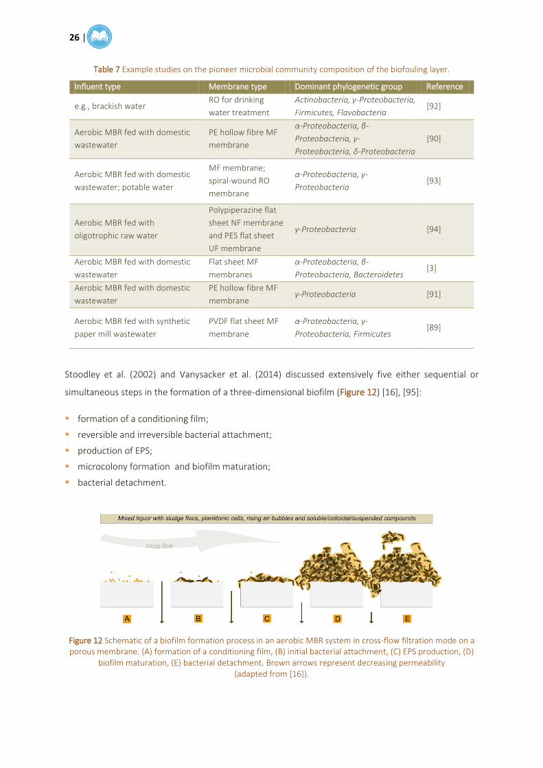
26 |

Table 7 Example studies on the pioneer microbial community composition of the biofouling layer.

Influent type Membrane type Dominant phylogenetic group Reference

e.g., brackish water RO for drinking

water treatment

Actinobacteria, γ-Proteobacteria,

Firmicutes, Flavobacteria [92]

Aerobic MBR fed with domestic

wastewater

PE hollow fibre MF

membrane

α-Proteobacteria, β-

Proteobacteria, γ-

Proteobacteria, δ-Proteobacteria

[90]


wastewater; potable water

MF membrane;

spiral-wound RO

membrane

α-Proteobacteria, γ-

Proteobacteria [93]

Aerobic MBR fed with

oligotrophic raw water

Polypiperazine flat

sheet NF membrane

and PES flat sheet

UF membrane

γ-Proteobacteria [94]


wastewater

Flat sheet MF

membranes

α-Proteobacteria, β-

Proteobacteria, Bacteroidetes [3]


wastewater

PE hollow fibre MF

membrane γ-Proteobacteria [91]

Aerobic MBR fed with synthetic

paper mill wastewater

PVDF flat sheet MF

membrane

α-Proteobacteria, γ-

Proteobacteria, Firmicutes [89]

Stoodley et al. (2002) and Vanysacker et al. (2014) discussed extensively five either sequential or

simultaneous steps in the formation of a three-dimensional biofilm (Figure 12) [16], [95]:

formation of a conditioning film;

reversible and irreversible bacterial attachment;

production of EPS;

microcolony formation and biofilm maturation;

bacterial detachment.

Figure 12 Schematic of a biofilm formation process in an aerobic MBR system in cross-flow filtration mode on a porous membrane. (A) formation of a conditioning film, (B) initial bacterial attachment, (C) EPS production, (D)

biofilm maturation, (E) bacterial detachment. Brown arrows represent decreasing permeability (adapted from [16]).

| 27

The first step in biofilm formation involves a physico-chemical change of the surface under

consideration (e.g., change in roughness or degree of hydrophilicity) [96] due to

adsorption/precipitation of particulate compounds or adhesion of dissolved substances onto the

surface, such as humic acids, proteins and carbohydrates present in the mixed liquor [6], [16].

The second step in biofilm formation, the initial bacterial attachment, is provoked by random collisions

of planktonic cells with the membrane surface [16] and an interplay between attractive van der Waals

and hydrophobic forces and mostly repulsive electrostatic interactions between the membrane

surface and the bacterial cell [97]. The bacterial attachment is then further promoted by interactions

between bacterial cells and between the bacterial cell and the membrane (e.g., via cellular surface

structures) [8].

The third step in biofilm formation is the production of extracellular polymeric substances (EPSs),

triggered by intra- and intercellular communication [8] EPSs are composed of various macromolecular

polyelectrolytes secreted by bacteria at or outside the cell surface. These biopolymers are mainly

carbohydrates and proteins of various molecular weights (typically from a few thousand to several

hundred thousand Daltons [98]) and at various ratios, but also lipids and nucleic acids are part of EPSs

[4], [6], [36], [53], [55], [58]. The exact composition is yet not known [67], but Xuang et al. (2000) and

Pollice et al. (2005) assumed it to be independent of the type of wastewater [61], [73]. These matrices

thus provides mechanic strength and protection against environmental stress factors (e.g., antibiotics,

pH changes) [16].

Vanysacker et al. (2014) reported that 400 articles were published between 1950 and 2014 on the role

of EPSs in membrane fouling [16]. However there exists a lot of discussion around the question

whether or not EPS have an influence on membrane fouling and at which extent [2], [25], [36], [48].

For instance Cho et al. (2002) stated that EPSs are important foulants [99] and Zhang et al. (2008)

attributed irreversible fouling to EPS adsorption [100], but there is uncertainty whether the

polysaccharides [7], [67] or the more hydrophobic proteins [27], [53] are the major contributors to

fouling. Two example studies illustrate this disagreement: Metzger et al. (2007) and Chen et al. (2006)

[82], [101].

The fourth step in biofilm formation involves microcolony development, thus reducing the overall flux.

A microcolony is defined as a cluster of cells on a surface, embedded in EPS, that has developed from

a single colonizing bacterial cell [8]. As the biofilm continues to grow, anoxic or anaerobic conditions

may develop in some parts of the biofilm and microniches may develop due to uneven spatial and

temporal distribution of nutrients inside the biofilm [16], thus enhancing colonization of the surface by

28 |

new bacterial species that ultimately intimately cooperate with the well-established species [8]. The

final architecture of the biofilm not only depends on the bacterial species, but also on the local flow

environment and the nutrient availability [8].

Finally the last step in biofilm formation is bacterial detachment from the biofilm. Detachment occurs

naturally (e.g., influenced by the physiology of the bacteria) or is provoked by human actions (e.g.,

membrane cleaning). Detached bacteria may start forming a biofilm elsewhere in the system [102].

3.3. Fouling stages

A long-term constant-flux filtration process seems to be characterized by a progressive increase of

resistance to filtration, translated in a time-dependent TMP increase (or similarly by a time-dependent

permeate flux decline) [85]. The time-dependency may be subdivided in two different regions (Figure

13), based on the critical flux concept as a central concept [56]. Pollice et al. (2005) considered the

critical flux value to determine the transition between reversible and irreversible fouling [61].

Figure 13 Typical fouling stages (adapted from [48]).

Field et al. (1995) distinguished Stage 1 and Stage 2 within the sub-critical region (i.e., when operating

a constant-flux filtration at a flux below the critical flux) [54].

Stage 1, also called ‘conditioning’ stage, consists of an initial short-term rapid linear rise in TMP

occurring in just a few hours, probably due to adsorption and precipitation of colloids and solutes

on the membrane surface and in the pores leading to pore blocking and closure [7], [48]. Stage 1

generally becomes less clear when membrane history becomes important (i.e., when the

membrane is not virgin anymore but already has undergone fouling and subsequently cleaning) [7].

Stage 2, also called ‘sustainable stage’, is characterized by a long and gradual linear or slightly

exponential increase in TMP up to the critical flux value [99]. This stage is mainly due to organic

precipitation and accumulation of EPSs present in the mixed liquor or produced by microorganisms

in the biofilm on the membrane surface or into the membrane pores [7], [48], [99].

| 29

Heterogeneous gradual pore closure and deposition of material at the membrane surface lead to

spatial variations in local fluxes along the membrane which could exceed the critical flux of the

suspension [61], [99]. At a certain point the supra-critical region is attained, the so-called Stage 3

where operation cannot be maintained for an extended period of time without severe fouling to

occur [7], [56], [61], [99]. Stage 3 is characterized by a sudden TMP jump. The cake layer gradually

loses porosity by compression [76]. Transfer limitation inside de cake layer finally result in death of

bacteria, thus more EPS release which further enhances fouling [39], [48], [53].

Zhang et al. (2006) reported that it may be desirable to limit the extent of Stage 1, to try to extend

Stage 2 as much as possible and definitely to avoid Stage 3 [7]. Unfortunately Cho et al. (2002)

reported that Stage 3 eventually occurs both in short-term filtration processes as in MBRs operated at

long term, even if filtration was performed at a flux below the critical flux [99]. However Pollice et al.

(2005) mentioned that Stage 3 arises more frequently in laboratory-scale set-ups [61]. Nevertheless

Fan et al. (2000), as cited by Ognier et al. (2009), managed to run a MBR continuously during 70 days

at a stable TMP that did equal four times the clear water TMP [58], [103].

3.4. Fouling control strategies

Zhang et al. (2006) discriminated between three interdependent parameters having an influence on

membrane fouling and sludge filterability (Figure 14) [7]:

the nature of the hydrodynamic environment;

the membrane properties;

the sludge characteristics, biopolymer concentration and microbial community structure, which in

turn are affected by operating parameters impacting on biomass growth and decay.

Field et al. (1995) introduced three approaches for the avoidance and remediation of fouling [54]:

the improvement of the hydrodynamics;

optimization of the membrane and process design;

periodic cleaning methods. Indeed, membrane fouling and biofilm formation are natural processes

that cannot be avoided completely [104]. Cleaning technologies can be divided into mechanical,

hydraulic, electrical and chemical methods [38], [105]. For an extensive review on membrane

cleaning methods in membrane bioreactors, please refer to Wang et al. (2014) [81].

These approaches may be combined to efficiently counteract fouling. As a reference, Zhang et al.

(2006) and Lee et al. (2007) reviewed studies focusing on specific fouling control strategies [7], [106].

The next sections highlight the effect of the hydrodynamic environment and the membrane and

process design.

30 |

Figure 14 Schematic of the factors affecting membrane fouling (adapted from [4], [7], [16], [42], [48], [52]).

3.4.1. Improvement of the hydrodynamics

Improvement of the hydrodynamics is inherently associated with decreasing the concentration

polarization and enhancing back transport of the deposited particles on the membrane surface into

the bulk mixed liquor [38]. This can be done in several ways.

Hydraulic cleaning methods involve intermittent operation modes such as back-flushing and/or

relaxation [52], [62], [107]. Back-flushing means the flux is reversed by switching the pressure so that

the permeate migrates in opposite direction through the membrane to the reactor for a limited

amount of time [4], [40]. On the contrary during relaxation the pressure is switched off for a limited

amount of time (i.e., TMP = 0), thus permitting the membrane and cake layer to relax, the latter

becoming more open. In the latter case the layer is removed by the turbulent forces across the

membrane surface and resuspended in the mixed liquor [4], [36], [38]. Back-flushing as well as

relaxation mode are standard anti-fouling strategies used in most of the MBR processes [27].

However, since both methods reduce the overall flux through the membrane (since the filtration

process is interrupted at discrete time moments, typically during 1-2 min every 8-10 min [4]), a

relatively high instantaneous flux must be applied in order to compensate for this loss. Wu et al.

(2008) and Metzger et al. (2007) reported the fouling behaviour to be more dependent on the

instantaneous flux than the filtration mode (continuous or intermittent mode) [27], [82]. Also the

duration, the interval and the strength of these hydraulic techniques were reported to influence the

fouling rate [27]. Finally the efficiency of hydraulic cleaning tends to decline with filtration time [5],

[27]. Thus a trade-off has to be made between permeation efficiency and fouling control [27].

| 31

Secondly hydrodynamic conditions can be improved by enhancing the shear forces along the

membrane by sparging coarse oxygen or air bubbles (> 3 mm) from the bottom of the bioreactor or

the membrane module (typically hollow fibres or flat sheets [4]) along the membrane surface, the so-

called ‘air-flush concept’ [38]. Judd (2008) stated that on approximation the membrane permeability

of submerged modules shows a linear increase with aeration rate [4]. Moreover this method has the

supplementary advantages to provide extra oxygen in the reactor mixed liquor by diffusion of oxygen

from the air bubble to the liquid [108] and to keep the biomass in suspension [5], [38]. It is however

important to determine the optimal packing density and distance between the modules in order to

optimize the air flow along the membrane surface [48], [62]. Finally it has been proven that there

exists a maximal aeration rate, above which no further significant fouling reduction is observed [5].

3.4.2. Optimization of the membrane design

The membrane design involves the adjustment of the membrane properties as to reduce the affinity

of the solutes with the membrane surface [54]. Stuckey (2012) distinguished three membrane surface

modifications: increase in hydrophilicity, alteration of the surface charge and bacterial anti-adhesion

modifications [42]. Liu et al. (2010) reported that a combination of these surface modifications yields

the best results for control and minimization of membrane biofouling [109].

Solutes and bacteria in the mixed liquor tend to show a greater affinity towards hydrophobic

membranes, as already mentioned previously in this chapter (Section 2.4.2). Thus it leads to more

severe fouling than hydrophilic membranes [5], [48], [88], [96], where the bacteria-membrane

interactions are mostly reversible [96]. Although research is being performed in order to increase

the hydrophilicity of hydrophobic membranes (e.g., [110] [111] [112] [113] [114] ), it has been

reported that the degree of hydrophilicity of a membrane is not a good indicator for biofouling

tendency; on the contrary the membrane surface charge plays a very important role [96], [109].

Moreover the degree of hydrophobicity of bacteria may even increase when attached onto the

membrane, as reported by Jinhua et al. (2006), thus enhancing further bacterial attachment [91].

The electrical properties of membrane surfaces can be modified with polycations or polyanions

[109]. Theoretically, electrostatic repulsion between the particles and the membrane surface will

occur if they bear the same charge, thus reducing fouling tendency by counteraction of the

attractive van der Waals forces [16], [78], [88]. However Pasmore et al. (2001) found that

biofouling is minimized when membranes are electrically neutral and increases with increasing

positive or negative charge [96]. This is most surprising since particles and bacteria must overcome

the electrical double layer formed in electrolytes and adjacent to the charged membrane surface

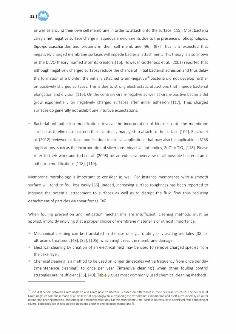
32 |

as well as around their own cell membrane in order to attach onto the surface [115]. Most bacteria

carry a net negative surface charge in aqueous environments due to the presence of phospholipids,

(lipo)polysaccharides and proteins in their cell membrane [96], [97] Thus it is expected that

negatively charged membrane surfaces will impede bacterial attachment. This theory is also known

as the DLVO theory, named after its creators [16]. However Gottenbos et al. (2001) reported that

although negatively charged surfaces reduce the chance of initial bacterial adhesion and thus delay

the formation of a biofilm, the initially attached Gram-negative28 bacteria did not develop further

on positively charged surfaces. This is due to strong electrostatic attractions that impede bacterial

elongation and division [116]. On the contrary Gram-negative as well as Gram-positive bacteria did

grow exponentially on negatively charged surfaces after initial adhesion [117]. Thus charged

surfaces do generally not exhibit one intuitive expectations.

Bacterial anti-adhesion modifications involve the incorporation of biocides onto the membrane

surface as to eliminate bacteria that eventually managed to attach to the surface [109]. Bazaka et

al. (2012) reviewed surface modifications in clinical applications that may also be applicable in MBR

applications, such as the incorporation of silver ions, bioactive antibodies, ZnO or TiO2 [118]. Please

refer to their work and to Li et al. (2008) for an extensive overview of all possible bacterial anti-

adhesion modifications [118], [119].

Membrane morphology is important to consider as well. For instance membranes with a smooth

surface will tend to foul less easily [36]. Indeed, increasing surface roughness has been reported to

increase the potential attachment to surfaces as well as to disrupt the fluid flow thus reducing

detachment of particles via shear forces [96].

When fouling prevention and mitigation mechanisms are insufficient, cleaning methods must be

applied, implicitly implying that a proper choice of membrane material is of utmost importance.

Mechanical cleaning can be translated in the use of e.g., rotating of vibrating modules [38] or

ultrasonic treatment [48], [85], [105], which might result in membrane damage.

Electrical cleaning by creation of an electrical field may be used to remove charged species from

the cake layer.

Chemical cleaning is a method to be used on longer timescales with a frequency from once per day

(‘maintenance cleaning’) to once per year (‘intensive cleaning’) when other fouling control

strategies are insufficient [36], [40]. Table 8 gives most commonly used chemical cleaning methods.

28 The distinction between Gram-negative and Gram-positive bacteria is based on differences in their cell wall structure. The cell wall of

Gram-negative bacteria is made of a thin layer of peptidoglycan surrounding the cytoplasmatic membrane and itself surrounded by an outer membrane bearing proteins, phospholipids and polysaccharides. On the other hand Gram-positive bacteria have a thick cell wall consisting of several peptidoglycan sheets stacked upon one another and no outer membrane [8].

| 33

Table 8 Most commonly used chemical cleaning agents for maintenance or intensive cleaning of membranes (based on [4], [38], [40], [48], [88]).

Chemical cleaning agent Example Purpose

Strong acids HCl, citric acid To break metal-associated structures, e.g., inorganic

precipitates and metal-organic complexes.

Enzymes Amylase, protease To destroy the cake layer.

Complexing agents EDTA, polyacrylates To remove organic and metal precipitates.

Disinfectants/oxidantia H2O2, NaClO To remove organic-based precipitation and

microorganisms.

Bases NaOH To remove organic foulants.

3.4.3. Optimization of the process design

Pollice et al. (2005) stated that increasing sludge concentration results in an exponential increase in

membrane fouling resistance during supra-critical operation [61], [71]. For instance as reported by

Yamamoto et al. (1989), when the MLSS concentration exceeds 40 000 mg l-1, the flux decreases

abruptly [68]. Indeed, since the MLSS concentration of the sludge suspension typically is several times

greater than the concentration of dissolved species [53], it may impact fouling by increasing the

dynamic viscosity of the mixed liquor [31]. Also high amounts of biopolymers (i.e., proteins,

carbohydrates) increase the viscosity of the sludge suspension so that the permeate flux through the

membrane is reduced and fouling is enhanced [72].

Process design can be optimized by adding non-ionic detergents and fouling reducers (adsorbents,

metal salts coagulants or flocculants) which may alter both the flocs and the mixed liquor supernatant

[38], [52], [62], [107]. Huyskens et al. (2012) reviewed literature about the effects of fouling reducers

[107]. The use of fouling reducers showed promising results in short-term experiments, but because of

their high cost [4], the uncertainty about the effect they have on the microbiology and their

environmental impact [48], it is uncertain they would show the same degree of success in long-term

applications.

Meng et al. (2006) stated that the particle size of sludge flocs, colloids and solutes present in the

mixed liquor has an influence on fouling [53]. When large sized particles (like flocs) attach to the

membrane, they tend to form a cake layer on the membrane surface. On the contrary, foulants which

are smaller (e.g., solutes) or of comparable size (e.g., colloids) than the membrane pores, will tend to

enter the pores and cause pore closure and pore blocking respectively. Thus fouling is greatly

influenced by the average sludge particle size distribution of the mixed liquor.

Influence of operating conditions

An important parameter to be considered in view of achieving long-term and sustainable operation is

the volumetric flux. High fluxes tend to enhance fouling by increasing convective transport of bacterial

cells and other particles to the membrane surface [3]. Thus, in order to decrease the migration of

34 |

bacterial cells and nutrients towards the membrane surface and to avoid compaction of the biofilm

[16], it is crucial to operate at a low ‘sustainable’ flux near the critical flux as to pursue a slow and

gradual TMP increase that can be maintained over a longer period [7], [52], [62], [107]. If high

productivities must be achieved, the low flux must be compensated by larger membrane areas [38].

Grelier et al. (2006) found membrane fouling in laboratory-scale experiments to be more dependent

on SRT than on MLSS concentration [2] and Huang et al. (2008) and Meng et al. (2009) designated the

SRT as the most important operating parameter in fouling phenomena [3], [48]. Short SRTs (< 10 days)

might result in an accumulation of biopolymers [4], [67] and a decrease of sludge filterability [2], thus

leading to high fouling rates and permeability decrease [4]. On the contrary divergent views exist on

the effect of high SRTs on membrane fouling. For instance Le-Clech (2010) and Massé et al. (2006)

stated that high SRTs generate higher MLSS concentrations in the form of smaller flocs and denser floc

aggregates, thus impeding oxygen transfer due to increased mixed liquor viscosity [5], [70]. Moreover

membrane fouling is enhanced by excessive development of filamentous bacteria [70]. On the other

hand some authors found that the biopolymer concentration tend to decrease at longer SRT (from 10

to 60 days) [2], [61], [67], thus leading to lower sub-critical fouling and increased wastewater

treatment efficiency [13]. Finally Judd (2008) evoked the advantage of promotion of slow-growers and

reduction of excess sludge production [4]. Based on Grelier et al. (2006) a SRT of 40 days shows

optimal membrane performance [2], but since full-scale plants are space-limited, a SRT between 15

and 40 days seems more appropriate, depending on the HRT and the feed solution [48].

Meng et al. (2007) investigated the effect of HRT on membrane fouling and stated that the HRT has an

indirect rather than a direct influence on fouling [31]. Decreasing HRTs result in lower DO

concentration due to the high biodegradation and thus oxygen utilization rate. Low HRTs moreover

result in a high F:M ratio, larger floc sizes, higher MLSS concentration and a higher sludge viscosity, all

of them influencing the oxygen transfer rate and the metabolic activity of the microorganisms.

Jeong et al. (2007) investigated the effect of the loading rate on bio-fouling and biopolymer

production rate and found that high loading rates resulted in a larger amount of attached substances

on the membrane surface [25] and higher fouling rates [120] caused by an increased sludge viscosity

and MLSS concentration [31].

Low temperatures produce a more viscous suspension thus slowing down diffusion of particles away

from the membrane surface and reducing the shear by air bubbles along the surface [60]. Low

temperatures also require higher driving forces in order to achieve the same flux [40]. Finally when

charged membranes are used in MBRs, their interaction with the charges on colloids or

macromolecules (e.g., proteins) is affected by pH-changes of the mixed liquor. The pH can also alter

inorganic precipitation of salts [48].

| 35

Chapter 3: Research methodology

The effect of the membrane morphology and more specifically the effect of membrane surface charge

on biofilm community structure and diversity, was assessed by means of two approaches:

Performance determination of the membranes based on physico-chemical related measurements

(ATR-FTIR, SEM, AFM, CAM, volume porosity measurement, electrokinetic characterization) and

permeability related measurements (CWP, critical flux);

Biofouling characterization based on molecular techniques (PCR-DGGE) and physico-chemical

techniques (ATR-FTIR, SEM, CLSM).

1. MEMBRANE AND MODULE PREPARATION

1.1. Membrane material

The homopolymer polyacrylonitrile (PAN) was chosen to synthesize hand-made

membranes to conduct the research on. The reasons are manifold. For instance

PAN is known to be thermally stable [121] and to have a high degree of

resistance against chemical cleaning agents (e.g., citric acid, CH3COOH, NaClO,

H2O2 and weak alkaline solutions such as NaOH) [45], [122]. Secondly Zhang et

al. (2008) reported that compared to other membrane materials, like PVDF, PSf or PES, the more

hydrophilic PAN membranes are more fouling-resistant [100]. Thirdly stable surface modifications are

much easier to achieve compared to e.g., PSf membranes [123]. Finally PAN can be used in a wide

range of full scale applications such as municipal and industrial wastewater treatment, biomedical

applications and concentration of proteins or oil/water mixtures [122], [123].

1.2. Membrane casting

16 flat-sheet membranes were prepared for the experiments, all having PAN as base structure:

Four neutral membranes containing no surface charges;

Four negatively charged membranes (hydrolysis);

Four positively charged membranes (hydrolysis followed by coating of 1 polymer layer);

Four negatively charged membranes (hydrolysis followed by coating of 2 different polymer layers).

Polyacrylonitrile

(PAN)

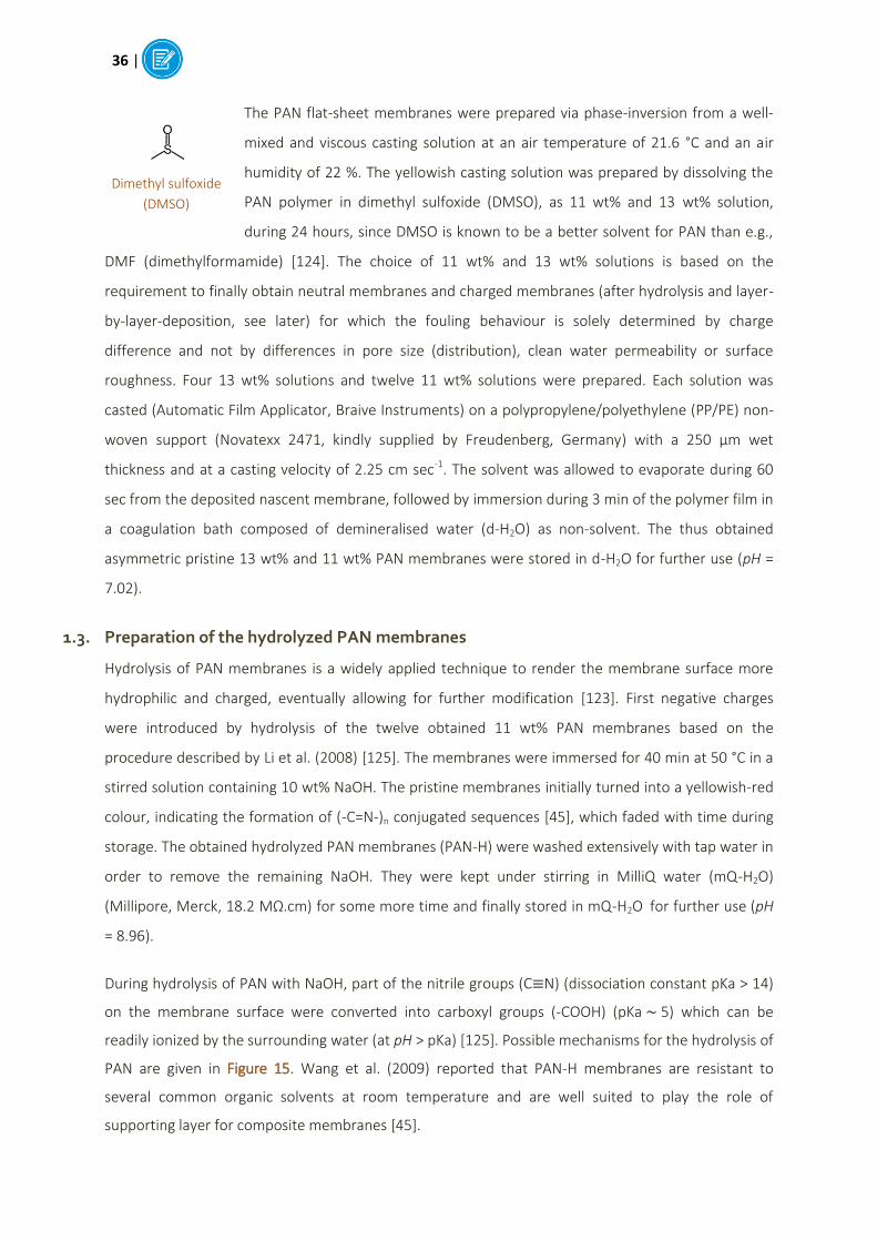
36 |

The PAN flat-sheet membranes were prepared via phase-inversion from a well-

mixed and viscous casting solution at an air temperature of 21.6 °C and an air

humidity of 22 %. The yellowish casting solution was prepared by dissolving the

PAN polymer in dimethyl sulfoxide (DMSO), as 11 wt% and 13 wt% solution,

during 24 hours, since DMSO is known to be a better solvent for PAN than e.g.,

DMF (dimethylformamide) [124]. The choice of 11 wt% and 13 wt% solutions is based on the

requirement to finally obtain neutral membranes and charged membranes (after hydrolysis and layer-

by-layer-deposition, see later) for which the fouling behaviour is solely determined by charge

difference and not by differences in pore size (distribution), clean water permeability or surface

roughness. Four 13 wt% solutions and twelve 11 wt% solutions were prepared. Each solution was

casted (Automatic Film Applicator, Braive Instruments) on a polypropylene/polyethylene (PP/PE) non-

woven support (Novatexx 2471, kindly supplied by Freudenberg, Germany) with a 250 µm wet

thickness and at a casting velocity of 2.25 cm sec-1. The solvent was allowed to evaporate during 60

sec from the deposited nascent membrane, followed by immersion during 3 min of the polymer film in

a coagulation bath composed of demineralised water (d-H2O) as non-solvent. The thus obtained

asymmetric pristine 13 wt% and 11 wt% PAN membranes were stored in d-H2O for further use (pH =

7.02).

1.3. Preparation of the hydrolyzed PAN membranes

Hydrolysis of PAN membranes is a widely applied technique to render the membrane surface more

hydrophilic and charged, eventually allowing for further modification [123]. First negative charges

were introduced by hydrolysis of the twelve obtained 11 wt% PAN membranes based on the

procedure described by Li et al. (2008) [125]. The membranes were immersed for 40 min at 50 °C in a

stirred solution containing 10 wt% NaOH. The pristine membranes initially turned into a yellowish-red

colour, indicating the formation of (-C=N-)n conjugated sequences [45], which faded with time during

storage. The obtained hydrolyzed PAN membranes (PAN-H) were washed extensively with tap water in

order to remove the remaining NaOH. They were kept under stirring in MilliQ water (mQ-H2O)

(Millipore, Merck, 18.2 MΩ.cm) for some more time and finally stored in mQ-H2O for further use (pH

= 8.96).

During hydrolysis of PAN with NaOH, part of the nitrile groups (C N) (dissociation constant pKa > 14)

on the membrane surface were converted into carboxyl groups (-COOH) (pKa 5) which can be

readily ionized by the surrounding water (at pH > pKa) [125]. Possible mechanisms for the hydrolysis of

PAN are given in Figure 15. Wang et al. (2009) reported that PAN-H membranes are resistant to

several common organic solvents at room temperature and are well suited to play the role of

supporting layer for composite membranes [45].

Dimethyl sulfoxide

(DMSO)

| 37

Figure 15 Possible mechanism for the hydrolysis of PAN with NaOH (reproduced from [123]).

In this research 11 wt% PAN membranes are hydrolysed instead of 13 wt% PAN membranes because:

11 wt% PAN yields a high porosity membrane after phase inversion compared to 13 wt% PAN;

membrane functionalization by hydrolysis results in a pore size reduction due to stretching of the

carboxylic groups under basic conditions, as reported previously [126].

Thus the non-modified (or neutral) 13 wt% PAN membranes and the hydrolysed (or negatively

charged) 11 wt% PAN-H membranes were expected to exhibit approximately the same pore size, what

will be confirmed further on during the experiments (Chapter 4, Section 2.1.2).

1.4. Layer-by-layer deposition: membrane functionalization

Eight out of the twelve PAN-H membranes did undergo surface modification by dipcoating in aqueous

solution of weak polyelectrolytes by means of manual layer-by-layer deposition.

The membranes were first immersed in a rinsing solution containing 0.05 M

NaNO3 in mQ-H2O (pH = 6) for 10 min, in order to wash the pores before the

polymer layer deposition. The wash step was followed by 30 min of dipping in an

aqueous solution of the polycation poly(allylamine hydrochloride) (PAH) (pKa =

8.7 [127]) with a concentration of 0.1 g in 1 l rinsing solution. The thus obtained

composite positively charged membranes (at pH < pKa) were then immersed again in the rinsing

solution for 2x 10 min in order to stabilize the adsorbed layer and to remove unadsorbed PAH and

thus preventing complexation of PAH and PAA in the next step [128]. The salt concentration has been

reported to have no significant effect on the assembly outcome [128]. Four out of the eight

membranes were stored in mQ-H2O for further use (pH = 8.45).

Poly(allylamine

hydrochloride)

(PAH)

38 |

The other four positively charged membranes continued the coating train with

the polyanion. After an additional 10 min immersion in the rinsing solution, they

were dipped for 30 min in a solution of 0.1 g poly(acrylic acid) (PAA) (pKa = 4.5

[129]) in 1 l rinsing solution. The thus obtained composite negatively charged

membranes (at pH > pKa) were then immersed again in the rinsing solution for 2x 10 min and finally

stored in mQ-H2O for further use (pH = 8.41).

1.5. Module potting

The obtained flat sheet membranes were potted into envelope-size modules (Figure 16). Each

membrane sheet was cut at the appropriate size and folded double to form an envelope surrounding

two sheets of spacer (3510 Corex, Agfa) and a permeate channel (silicon tube), meant to connect the

module interior to the peristaltic pump of the reactor. Each folded membrane was fixed to a PVC

frame (Bonte Ateliers, Leuven) by glueing the edges together using a 50/50 mixture of binder and

hardener (UHU plus, endfest 300, Germany). The glued edges were allowed to dry overnight while

keeping the membranes wet.

Figure 16 Structure of the envelope-sized modules. (1) double folded membrane sheet, (2) spacer sheets, (3)

permeate channel, (4) PVC frame.

The final modules (Figure 17) had an effective filtration area of 2x 75 cm² and were stored in d-H2O for

further use.

Figure 17 Final modules and their respective surface charges. (A) 13% PAN – neutral, (B) 11% PAN (-) – hydrolyzed, (C) 11% PAN (+) – 1 deposited layer PAH, (D) 11% PAN (-) – 2 deposited layers PAH & PAA.

Poly(acrylic acid)

(PAA)

| 39

2. OPERATING CONDITIONS OF THE LAB-SCALE MBR SYSTEM

2.1. Membrane bioreactor design

2.1.1. Laboratory-scale high-throughput membrane bioreactor

Fouling experiments were conducted using a laboratory-scale high-throughput membrane bioreactor

(HT-MBR) (Figure 18) composed of an aerated bioreactor tank with a volume of 37.8 l which contained

the 4x four replicate membrane modules immersed in clusters of 4 different membrane types in 20 l

activated sludge.

Figure 18 Schematic of the HT-MBR. (1) feed tanks, (2) feed pump and level controller, (3) bioreactor containing the 4x 4 replicate membrane modules immersed in activated sludge, (4) permeate pump, (5) air supply. The upper right figure represents the clustered arrangement of the membrane replicates inside the bioreactor.

The permeate was sucked through a multichannel peristaltic pump (Watson Marlow, 205U) connected

to the 4x four replicate modules and at an average total constant cross-flow rate of (25.6 3.1) l day-

1, corresponding to 6.5 LMH per membrane, using cycles of 8 min filtration and 2 min relaxation

without back-flush, as done by e.g., Piasecka et al. (2012) [6]. The use of moderate permeation and

relaxation times allows for control of local instantaneous fluxes across the membrane thus mitigating

fouling [27]. The MBR was fed (Watson Marlow, 503S) with a protamylasse solution as to keep the

sludge suspension volume constant by means of a level controller. 1.4 l sludge suspension was

withdrawn manually from the reactor weekly to control the sludge retention time (SRT) and total

solids concentration (TS). The MBR was operated at a SRT of 100 days and an average hydraulic

retention time (HRT) of 18.75 hours. The SRT is defined as:

SRT =

Equation 9

40 |

Where V (m³) is the working volume of the reactor and Qsludge (m³ day-1) is the rate at which sludge is

removed from the reactor [11]. The longer the SRT, the longer the contact time between bacteria and

organic molecules, thus the higher the biodegradation [11], [70]. A SRT of 100 days is higher than

generally reported in literature for the treatment of municipal wastewater, i.e., typically between 5

days [13] and 60 days [76], but since the HT-MBR here was operated on protamylasse wastewater

(industrial origin), a SRT of 100 days is most common. For instance, Piasecka et al. (2012) reported to

work with molasses wastewater (from alcohol distilleries) at a non-limiting SRT (i.e., no sludge

withdrawal except for sampling) [6]. The HRT is defined as:

HRT =

Equation 10

Where V (m³) is the volume of the reactor and Qfeed (m³ h-1) is the rate at which the reactor is fed. The

HRT thus is a measure for the time needed by the liquid phase to migrate through the reactor [4]. A

HRT of 18.75 hours is relatively high compared to HRTs previously reported for the treatment of

municipal wastewater, e.g., varying between 5 hours [13] and 12 hours [2], [76]. Since the HT-MBR

here was operated on protamylasse wastewater, a HRT of 18.75 hours is most common, like reported

by Piasecka et al. (2012) or Bilad et al. (2011) who operated their MBR on molasses wastewater with a

HRT of 18-20 hours [6], [130].

The MBR was aerated at a constant rate of 10 LPM (l min-1) (i.e., 0.6 m³ h-1) unfiltered compressed air

at a pressure of 3.25 bar (Variable Area Flow Meter EK-4BR, Kytola Instruments), which is in the range

of reported aeration rate values, e.g. values as low as 0.2 m³ h-1 [2], [53], [76] and as high as 1.2 m³ h-1

[3], [27]. The air was introduced in the reactor by means of coarse bubbles rising from perforated

pipes underneath the membrane modules to provide oxygen and turbulent mixing.

Finally the temperature was monitored four times a week and fluctuated between 10.5 °C and 16.2 °C

according to variations in room temperature since no heat control was applied.

2.1.2. Origin of activated sludge and feed

The bioreactor was inoculated with 20 l aerobic activated sludge collected from the sedimentation

tank of the local wastewater treatment plant of Leuven, Aquafin.

During the first 17 days, the HT-MBR was operated on 1.5 ml l-1 protamylasse feed (AVEBE, Veendam,

The Netherlands) diluted in tap water. From day 18 on, the concentration was increased up to 2.3 ml l-

1 as to control sludge bulking. The concentration was comparable to the one used by Bilad et al. (2010)

| 41

and Bilad et al. (2011) for the operation of a HT-MBR on molasses wastewater (i.e., 2.25 ml l-1) [130],

[131]. Protamylasse can be defined as a protein-free potato-juice, a brownish and viscous residue of

the industrial starch industry, containing a range of compounds necessary for microbial growth (Table

9). As seen from the table, the feed solution contains a pH-buffer (KH2PO4) thus influent pH was

adjusted to neutral pH and had a value of (6.90 0.25) throughout the experiments.

Table 9 Average composition of the protamylasse residue (54% dry weight) (adapted from [132]).

Composition Concentration (g l-1

)

Amino acids Total: 183.0

Mainly: Asparagine 65.1 Glutamine 39.7

Organic acids Total: 135.2

Citric acid 76.3 Oxalic acid 6.1 Lactic acid 13.2

Malic acid 35.6 Acetic acid 4.1

Sugars Total: 142.3

Glucose 35.6 Fructose 35.6 Saccharose 71.2

Salts and minerals Total: 225.7

K+

97.6 Na+

0.8 Cu2+

0.04

PO43-

25.4 NH4+

4.0 Cl-

8.1

Mg2+

4.5 Mn2+

0.03 NO3-

2.2

Ca2+

0.6 Zn2+

0.08 SO42-

22.4

2.1.3. Maintenance of the HT-MBR

The reactor was inoculated with sludge on the 15th of September 2014 (Day 1) (Figure 19). First the

sludge suspension was acclimated to the MBR system using random PVDF membranes for 72 days as

to obtain stable operation before starting the fouling experiments, hereafter called ‘Transient Period

1’. During this transient period, the feed pump did stop working several times thus perturbing stability.

The 4x four replicate modules were immersed in the reactor on the 25th of November 2014 (Day 72),

hereafter called ‘pristine membranes (P-membranes)’. On the 3rd of January 2015 (Day 111), after 39

days stable operation, hereafter called ‘Fouling Period 1’, the fouling experiment ended abruptly due

to feed pump malfunctions. The membrane modules were removed from the reactor and cleaned

thoroughly using a three-step protocol in order to remove the hardened and dried fouling cake on

their surfaces: (i) washing with tap water during 5 min to remove loosely attached material, (ii)

submerging intermittently in 2 ‰ NaClO (pH 10.55) in d-H2O during a total of 3.5 days, (iii) rinsing with

d-H2O during 5 min to remove the cake residues and the residual NaClO. The NaClO solution was

changed every day in order to maintain a constant chlorine concentration. The modules were filtered

with mQ-H2O (as explained in Section 3.3.2) and stored in d-H2O for further use.

42 |

The reactor was run for 40 days using random PVDF and PVC/silica membranes as to obtain stable

operation again before restarting the fouling experiments, hereafter called ‘Transient Period 2’. During

this transient period, the feed pump did stop working several times.

The cleaned replicate modules were immersed back in the reactor on the 12th of February 2015 (Day

151), hereafter called ‘cleaned membranes (C-membranes)’. On the 23rd of March 2015 (Day 190),

after 39 days stable operation, hereafter called ‘Fouling Period 2’, the fouling experiment was ended.

Figure 19 Timeline of the fouling experiments.

None of the equipment was sterile or autoclaved during use. The modules were not cleaned

chemically or mechanically during the fouling periods. Only the protamylasse feed containers and the

PVC tubes transporting the feed solution to the bioreactor vessel were thoroughly cleaned with 1 ‰

NaClO (15° chlorine) during 30 min and rinsed with tap water during 5 min every week during both

transient periods and fouling periods. The period between two cleaning moments, hereafter called

‘maintenance period’, thus lasted 8 days.

2.2. Quality measurements

2.2.1. Operational parameters

During both the transient periods and the fouling periods, the total solids (TS), the mixed liquor

(volatile) suspended solids (ML(V)SS), the sludge volume index (SVI) and pH were monitored (pH-

Meter 330, WTW) two times a week by taking uniform sludge samples from the middle zone of the

bioreactor. The dissolved oxygen concentration (DO) (pH/Oxi 340i, WTW) was recorded only at the

end of Fouling Period 2 since the measurement equipment was not available earlier.

The TS concept (g l-1) (expressed in dry weight) has already been introduced before as the

concentration of suspended and dissolved solids present in the wastewater (Chapter 2, Section 1.1.1).

It was measured by drying 3 ml activated sludge suspension in the oven (Memmert) during 2 h at 105

°C to constant weight and calculating the difference between wet and dry sample [11]. Measurements

were performed in triplicates.

| 43

The total suspended solids (TSS) or MLSS concentration (g l-1) (expressed in dry weight) is defined as

the concentration of suspended solids present in the wastewater. Its evolution with time is an

indication of biomass growth [6]. It is obtained after filtration of the sludge suspension through a 0.22

µm or 0.45 µm filter paper and subsequently drying the filter residue in the oven at 105 °C during 2 h

to constant weight [11], [108]. The MLSS is obtained by calculating the difference between wet and

dry sample. Here the TS concentration is used as approximation for the MLSS concentration.

The volatile suspended solids (VSS) or MLVSS concentration (g l-1) (expressed in dry weight) represents

the organic fraction of the suspended solids in the wastewater. It is an approximation for the

concentration of active biomass. It was measured by drying 3 ml activated sludge in the oven

(Memmert) during 2 h at 105 °C to constant weight, followed by ashing the residue in the muffle oven

(B 180, Nabertherm) at 550 °C during 3 h. The MLVSS was then calculated as: MLVSS = MLSS – ash

[11], [108]. Measurements were performed in triplicates.

The SVI (ml g-1) is an empirical measure for the settleability and flocculation state of activated sludge

[49]. It is defined as the total volume (ml) occupied by 1 g of MLSS after 30 minutes of sedimentation.

Good settling sludge has a SVI equal to or less than 100 ml g-1 (expressed as dry weight), while bulking

sludge (Chapter 2, Section 1.2.2) occurs at a SVI exceeding 150 ml g-1 (expressed as dry weight) [28]. In

the latter case the diluted sludge volume index (DSVI) (ml g-1) is a better measure [11]. The settled

volume was measured in twofold replicates in 100 ml graduated cylinders. The SVI was calculated

according to:

SVI =

Equation 11

2.2.2. Physico-chemical analysis

During both the transient periods and the fouling periods, parameters for the measurement of organic

pollution (COD) and parameters for the measurement of nutrient concentrations (TN, phosphate)

were monitored once every two weeks by taking uniform sludge samples from the middle zone of the

bioreactor, as well as feed wastewater samples and permeate samples from the outlet of the

peristaltic tubes.

The concepts of Chemical Oxygen Demand (COD), total nitrogen (TN) and phosphate have already

been introduced before (Chapter 2, Section 1.1.1). The concentrations were measured using Hach-

Lange kits on the appropriate dilutions in tap water (Table 10) (LCK 314: 2.5 mg l-1, LCK 138: 0.26

mg l-1 and LCK 349: 0.03 mg l-1 respectively) supported by Hach-Lange equipment (LT 200 Dry

44 |

thermostat and DR 1900 Portable spectrophotometer). No distinction was made between nitrogen

species during the measurements (NO3- -N, NO2

- -N, NH4+ -N). Also the soluble COD (sCOD) of the

sludge suspension were determined by filtering the liquid through a 0.45 µm polyester-filter

(Chromafil® PET-45/15 MS, Macherey-Nagel), as adapted from [70]. No replicates were used.

Table 10 Hach-Lange measurements performed on permeate, sludge and protamylasse feed solution samples.

Sample Dilution COD29

TN30

phosphate31

Permeate

/ X

10x X

20x X

Feed solution 25x X X X

Sludge suspension, filtered 3x X

The measured concentrations were used to calculate the COD:N:P ratio of the protamylasse feed

solution and permeate as well as removal efficiencies. The removal efficiency (%), representing the

relative concentration difference between reactor influent and effluent, was calculated as:

RE =

* 100 Equation 12

Where Ci is the concentration in the influent and Ce is the concentration in the effluent [11].

Finally the average COD concentration of the feed was used to determine the sludge loading rate and

the volumetric loading rate. The sludge loading rate (Bx) (kg COD kg-1 MLSS d-1), also designated as the

food-to-microorganism ratio (F:M), represents the amount of substrate given daily to the

microorganisms. The volumetric or organic loading rate (Bv) (kg COD m-3 d-1) was already introduced

before (Chapter 2, Section 1.3.2). The volumetric loading rate is expressed per reactor volume (m³) and

is calculated according to [11]:

Bv = MLSS * Bx Equation 13

2.2.3. Microscopic analysis

The sludge composition and floc structure and size were analyzed microscopically (BX51, Olympus)

with a 10x zoom magnification and by means of the objectives UPlanFI 100x/1.30 oil Ph3 ∞/0.17

(magnification 100x), UPlanFI 40x/0.75 Ph2 ∞/0.17 (magnification 40x) and UPlanFI 10x/0.30 JAPAN

(magnification 10x) every two weeks in order to assess the quality and state of the sludge biomass and

29 measurement range: 15-150 mg l-1 30 measurement range: 1-16 mg l-1 31 measurement range: 0.05-1.50 mg l-1

| 45

the presence of microorganisms other than bacteria in view of rapid process optimization (e.g.,

organic loading, aeration). The microscope images (analySIS®, Soft Imaging System GmbH, Germany)

at a magnification 100x were used to quantify the number of filamentous bacteria by means of the

arbitrary Filament Index (FI). The FI has a scale between 0 and 5, representing none to very many

filaments, and is determined based on a series of reference images as explained by Eikelboom (2000)

[28]. Microscopic analysis was also performed every two weeks on the permeate and during three

maintenance periods of 8 days on the protamylasse feed solution in order to assess the presence of

bacteria or other micro-organisms.

3. MEMBRANE PERFORMANCE MEASUREMENT

Since the structural properties of membranes used in the MBR influence the membrane separation

process and the (bio)fouling phenomena, it is essential to collect information on the membrane

characteristics (e. g., surface groups, top layer thickness, pore size, surface charge, surface roughness,

degree of hydrophilicity/hydrophobicity, permeability, etc.). Two types of characterization methods

can be distinguished, the latter being considered as a validation method for the former [37]:

Physico-chemical related measurements

Permeability related measurements

3.1. Membrane sampling

Physico-chemical related measurements were performed on membrane disks or coupons with an area

of 1.77 cm² cut out of the membrane sheets. Permeability related measurements were performed (i)

on membrane disks or coupons with an area of 1.77 cm² cut out of the membrane sheets or (ii) on the

membrane modules. Unless specified otherwise, all measurements were performed on P-membranes

(Section 2.1.3).

3.2. Physico-chemical related measurements

3.2.1. Attenuated Total Reflectance Fourier Transform Infrared Spectroscopy

Attenuated Total Reflectance Fourier Transform Infrared Spectroscopy (ATR-FTIR) allows

determination of the functional groups present at the membrane surface, by collecting an infrared

spectrum in the range 4000-370 cm-1 and assigning chemical bonds to typical vibration typologies.

Two coupon replicates per membrane type were air-dried during 24 h to remove the majority of the

water, followed by drying in a vacuum oven (Sheldon Manufacturing 1410, VWR International) at 29

Hg.vac (i.e., 50 mbar) (Mad.Duo2, Pfeiffer Vacuum) at room temperature during 6 h prior to analysis,

46 |

in order to minimize IR absorbance due to water present in the sample which could occur other peaks.

After drying, the coupons were stored in closed recipients partly filled with cobalt chloride desiccants

pending the measurements. The IR spectra were collected by measurements at room temperature on

2 to 4 points per coupon replicate using a FTIR spectrometer (Alpha-P, Bruker Corporation) and

baseline corrected with optical spectroscopy software (OPUS, Bruker Corporation). ATR-FTIR

measurements were performed on both the P- and the C-membranes in order to investigate the

effect of long-term cleaning with NaClO. The IR spectra of the C-membranes are presented in Section

2.1.1 of Appendix 1.

3.2.2. Scanning Electron Microscopy

Scanning Electron Microscopy (SEM) allows determination of the surface structure and membrane

morphology (top layer thickness, cross-section, porosity [37]) by means of electrons accelerated

towards the membrane sample and backscattered to a detector, which records depth and surface

information, thus yielding a two- or three-dimensional image of the sample [133].

A coupon of each membrane type was air-dried for 24 h and cut (surface analysis) or fractured

manually (cross-sectional analysis). No liquid nitrogen was required since PAN is naturally very brittle

in its dry state. The membrane samples were mounted on a SEM-holder by means of double-sided

adhesive tape. Samples meant for surface analysis were coated with a thin layer of a mixture of gold

and palladium (Sputtering Device 07120/172, Balzers Union) prior to analysis. Samples meant for

cross-sectional analysis were coated with a thin layer of gold (Auto Fine Coater JFC-1300, JEOL USA).

The membrane surface structures were analyzed using a scanning electron microscope (SEM XL30

FEG, Philips) and imaging software (XL30 Microscope Control) at an accelerating voltage of 10 kV and

magnifications 1500x and 10 000x as well as at 12 kV and magnification 50 000x. The membrane

cross-sections were analyzed using a scanning electron microscope (JSM-6010 LV, JEOL USA) and

imaging software (InTouch, JEOL USA) at an accelerating voltage of 10 kV and magnifications 300x,

330x or 350x and 3000x or 3500x. SEM measurements were performed on both the P- and the C-

membranes in order to investigate the effect of long-term cleaning with NaClO. The SEM images of

the C-membranes are presented in Section 2.1.2 of Appendix 1.

3.2.3. Atomic Force Microscopy

Atomic Force Microscopy (AFM) allows determination of the three-dimensional micro-topography of

the membrane surface (to atomic resolution [134], [135]) based on attractive forces (hydrogen

bonding, van der Waals) and repulsive forces (electrostatic) between the scanning probe and the

membrane surface [24], [133] It is often used as complementary technique to SEM [44], [78].

| 47

Measurements were performed in collaboration with Prof. Dhr. Alexander Volodin for the Department

of Physics and Astronomy of the KUL. One coupon of each membrane type was air-dried during 24 h

prior to analysis. Measurements were performed in dry state at three different locations per coupon

as to take into account local heterogeneities of the membrane surface. Scans were performed at

tapping mode using a scanning probe microscope (PicoPlus – AFM, Series 5500, Agilent Technologies

Inc., USA) and thus allowing minimal deformation of the surface topography of the dried membranes

[44]. Silicon tips (Pointprobe-Plus® Silicon-SPM-Sensor, Nanosensors, Germany) hold by a cantilever

with a thickness of (2.0 1) µm, a resonance frequency of 6-21 kHz and a force constant of 0.02-0.77

N m-1 were used at a tip height of 10-15 µm. The images were flattened (1st order) in order to exclude

the long-wave variations related to the substrate. The membrane surface roughness was determined

from 1x1 µm and 10x10 µm areas at each location and reported in terms of the root mean square

height, Rms (nm) [121], [125]:

Rms =

Equation 14

With n the locations per coupon, Zi (nm) the height at location i and (nm) the average height of the n

data points.

3.2.4. Contact Angle Measurement

Contact Angle Measurements (CAM) allow determination of the degree of

hydrophilicity/hydrophobicity of chemical groups attached to the outer layer of a membrane surface

by measurement of the wetting or contact angle formed between the solid surface and the line

tangent to the surface of the droplet used for the analysis. A contact angle of less than 90 degrees

represents a hydrophilic surface, while a contact angle between 90 and 180 degrees represents a

hydrophobic surface [98].

Two coupon replicates of each membrane type were air-dried for 24 h prior to analysis. Contact angles

were measured by placing one drop of d-H2O with a volume of 2 µl at 3 locations per coupon replicate

with a dropper at room temperature. Directly after placing the droplet on the membrane surface, a

camera recorded the time-evolution of the drop from the side view, followed by on-line

measurements of the contact angle on both sides of the drop (left and right angle, as measure for the

droplet uniformity) by a goniometer (DSA 10-MK2, Krüss). These measurements were averaged out to

yield the average contact angle (ϑ-value).

48 |

3.2.5. Volume porosity measurement

Water uptake measurements based on the method described by Panda et al. (2015) were performed

to determine the swelling potential and volume porosity of the P-membranes [121]. Two coupon

replicates per membrane type were immersed in d-H2O immediately after synthesis during a non-

limiting amount of days (> 72 h) followed by oven-drying at 60°C during 24 h. The oven temperature

would not alter the chemical structure of the membranes since the glass transition temperature of

PAN is 85 °C [45], 106 °C for PAA and around 90 °C for PAH [136] . The water uptake results, calculated

as a water mass loss after drying, were used to determine the volume porosity of the membranes ( ),

using following relationship [121]:

(%) =

=

* 100 Equation 15

With Vvoids (m³) the pore volume of the membrane, Vtotal (m³) the total volume of the membrane, ρw =

1 000 000 g m-3 the water density at room temperature, A = 0.000314 m² the membrane surface area

and x = 0.0005 m the membrane thickness (non-woven support + porous membrane). mwet (g) and

mdry (g) are the mass of the wet and air-dried membrane coupon respectively. The wet membrane

mass was obtained by removing the excess water from the surface of the membrane coupons with

filter paper. The effect of the Novatexx non-woven support was taken into account by subtracting its

water mass uptake from the measurements.

3.2.6. Electrokinetic characterization

Zeta (ζ) potential or surface electric potential measurements [137] allow for the determination of the

surface charge density of membranes [115] and is calculated based on the relative migration of a

colloidal suspension with varying pH along the membrane surface [133]. The ζ-potential values are

highly dependent on surface characteristics of the membranes (e.g., functional groups, wettability,

roughness), on the properties of the electrolyte solution used for the measurements (e.g.,

concentration, pH, valence of ions) and measurement conditions (e.g., temperature) [137]–[139].

Measurements were performed in collaboration with Prof. Dhr. Anthony Szymczyk from the Institut

des Sciences Chimiques de Rennes (France). The apparent ζ-potential can be determined based on

measurements of the tangential streaming current, induced by a hydrostatic gradient, and which

represents the amount of charged particles that flow along the membrane surface and their

subsequent accumulation downstream of the membrane [133], [137]. One pair of coupon replicates

per membrane type, stored in d-H2O prior to analysis, was mounted as a channel in a streaming

potential cell (SurPASS Electrokinetic Analyzer, Anton Paar) at a channel height or inter-membrane

| 49

distance of (95 5) µm. An electrolyte solution of 0.001 M KCl was pumped through the cell at room

temperature based on hydrostatic pressure increments from 0 to 300 mbar. The pH of the electrolyte

solution was adjusted between 3 and 8 by means of 0.1 M HCl and 0.1 M KOH solutions. The

electrokinetic behaviour of the membrane samples was analyzed under N2 inert atmosphere and the

streaming current was monitored by Ag electrodes coated with AgCl. Data acquisition took place by

means of the Visiolab software. The relationship between the streaming current, Is (A), and the ζ –

potential (V) is given by the Helmholtz-Smoluchowski equation [115], [137], [140]:

= -

Equation 16

With W (m) the channel width, hch (m) the channel height, 0 the vacuum permittivity (8.854E-12 F m-

1), r (-) the dielectric constant of the electrolyte solution, ΔP (N m-2) the hydrostatic pressure, (kg m-

1 s-1) the viscosity of the electrolyte solution and L (m) the channel length. The determination of the

surface charge density based on ζ-potential values is done as explained by Schaep et al. (2001) [115].

3.3. Permeability related measurements

3.3.1. Clean water permeance of membrane coupons

The clean water permeance (CWP) (LMH bar-1) is defined as the maximum flux per unit TMP that the

membrane can achieve in the absence of (bio)fouling [37].

The CWP of three membrane coupon replicates per membrane type was assessed at room

temperature by means of a stainless steel high throughput device (HT pressure driven liquid

separation, in collaboration with Agila) running 16 dead-end filtrations in parallel at a constant

pressure of 1.3 bar (Nuova Fima) using mQ-H2O (Figure 20).

Figure 20 High-throughput device for the CWP measurement of membrane coupons.

The feed water was stirred at 500 rpm during filtration. After a compression period of 15 min the

permeate of each coupon was collected in vials in triplicate. The CWP of each membrane type

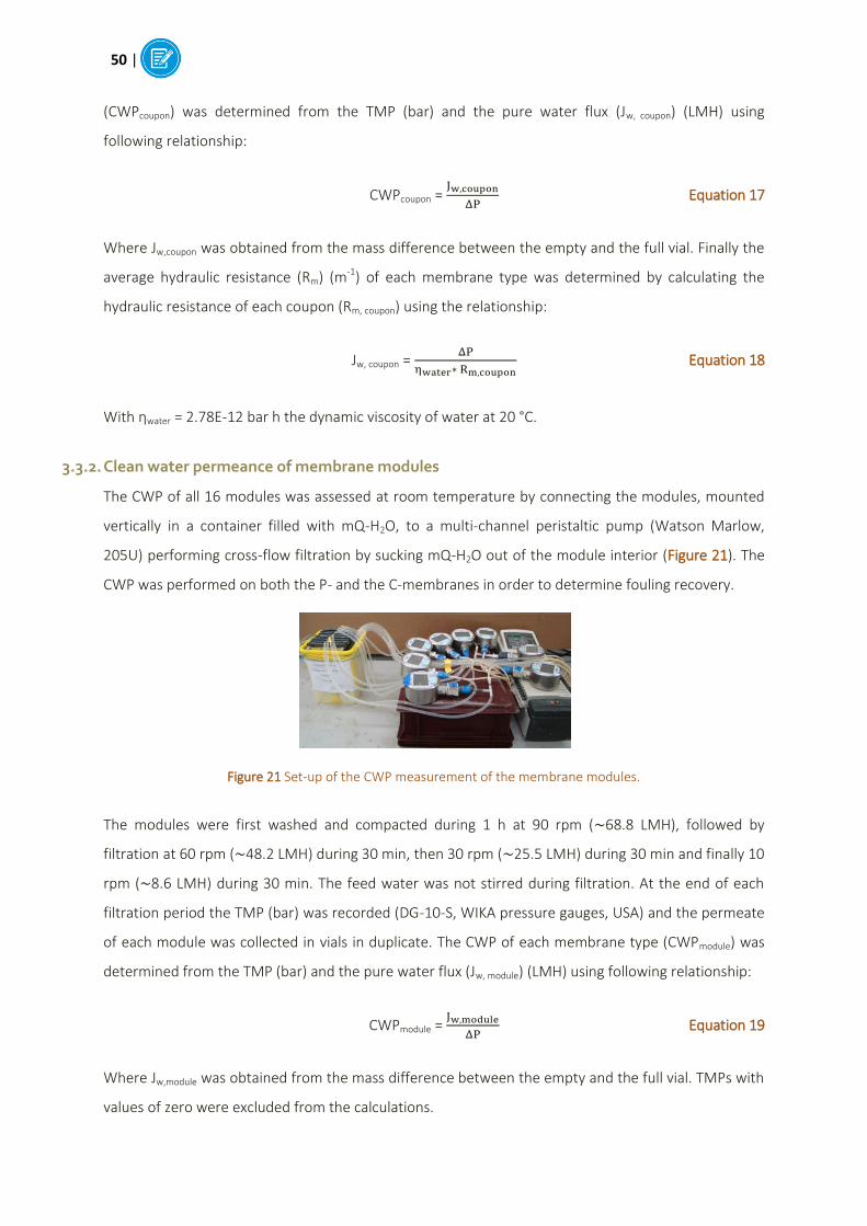
50 |

(CWPcoupon) was determined from the TMP (bar) and the pure water flux (Jw, coupon) (LMH) using

following relationship:

CWPcoupon =

Equation 17

Where Jw,coupon was obtained from the mass difference between the empty and the full vial. Finally the

average hydraulic resistance (Rm) (m-1) of each membrane type was determined by calculating the

hydraulic resistance of each coupon (Rm, coupon) using the relationship:

Jw, coupon =

Equation 18

With water = 2.78E-12 bar h the dynamic viscosity of water at 20 °C.

3.3.2. Clean water permeance of membrane modules

The CWP of all 16 modules was assessed at room temperature by connecting the modules, mounted

vertically in a container filled with mQ-H2O, to a multi-channel peristaltic pump (Watson Marlow,

205U) performing cross-flow filtration by sucking mQ-H2O out of the module interior (Figure 21). The

CWP was performed on both the P- and the C-membranes in order to determine fouling recovery.

Figure 21 Set-up of the CWP measurement of the membrane modules.

The modules were first washed and compacted during 1 h at 90 rpm ( 68.8 LMH), followed by

filtration at 60 rpm ( 48.2 LMH) during 30 min, then 30 rpm ( 25.5 LMH) during 30 min and finally 10

rpm ( 8.6 LMH) during 30 min. The feed water was not stirred during filtration. At the end of each

filtration period the TMP (bar) was recorded (DG-10-S, WIKA pressure gauges, USA) and the permeate

of each module was collected in vials in duplicate. The CWP of each membrane type (CWPmodule) was

determined from the TMP (bar) and the pure water flux (Jw, module) (LMH) using following relationship:

CWPmodule =

Equation 19

Where Jw,module was obtained from the mass difference between the empty and the full vial. TMPs with

values of zero were excluded from the calculations.

| 51

Finally the average hydraulic resistance (Rm,P-module) (m-1) for P-membranes and the average resistance

after cleaning Rm,C-module (m-1) for C-membranes was determined for each membrane type by

calculating the hydraulic resistance of each module using the relationships:

Jw, module =

or Jw, module =

Equation 20

With water = 2.78E-12 bar h the dynamic viscosity of water at 20 °C.

3.3.3. Critical flux determination

The theory of critical flux was already extensively explained previously (Chapter 2, Section 2.2.7). The

most widely used methodology to assess the critical flux value and the short-term fouling rate, is the

TMP measurement in flux-stepping experiments during constant-flux filtration on membrane modules

with activated sludge, performed in the MBR. Due to a personal error, the critical flux measurement

was performed on the C-membranes instead of the P-membranes. Thus the critical flux values of the

pristine membranes were extrapolated from the results obtained based on the cleaned membranes.

Based on an adaptation of the methodology used by Le Clech et al. (2003), van der Marel et al. (2009),

Pollice et al. (2005) and Cho et al. (2002), the flux-stepping experiment was performed with flux steps

of 30 min, involving 20 min filtration (Watson Marlow, 205U) and 10 min relaxation [59]–[61], [99]. An

arbitrary maximum flux scale of 50 rpm ( 35.0 LMH) was reached starting from an initial flux scale of

5 rpm ( 3.5 LMH) and with a flux step height of 5 rpm ( 3.5 LMH). The corresponding TMP was

recorded every 5 min (DG-10-S, WIKA pressure gauges, USA).

Two different figures were obtained based on the collected results. Firstly a graph, summarizing the

experimental data, was plotted to represent the TMP (mbar), averaged over the modules of the same

membrane type, and the flux (LMH) against time (min). Secondly, the average fouling rate dΔP/dt

(mbar h-1) was plotted against the flux (LMH). From the figure, the (apparent) critical flux (Jc) could be

determined. Jc is defined as the maximum flux above which deviation from the linear trend occurs by

calculation of

[59]. Alternatively the determination of Jc could be based on arbitrary threshold

values like a threshold fouling rate of 0.1 mbar min-1 [59] or a threshold permeance change K > 0.9 K0,

with K0 the permeance during the first flux step [55]. Threshold values are necessary to determine Jc

since fouling does always occur during MBR operation with activated sludge [59] [60]. The effect of

temperature on the critical flux value was minimized by correction of Jc based on following empirical

formula from [141]:

52 |

JcT = Jc

20 * 1.025(T-20) Equation 21

Where JcT and JC

20 are the critical flux values at a sludge temperature T = 14.2 °C during the

measurements and at 20°C respectively.

4. BIOFOULING (COMMUNITY) CHARACTERIZATION

Meng et al. (2010) considered MBR fouling as a Black Box, despite the many efforts to correlate the

fouling mechanism to influences of membrane materials, sludge characteristics and operating

conditions [24]. They identified three approaches to unravel the mysteries around fouling:

Microbiological identification

Morphological visualization of the fouling layer

Chemical characterization of the foulants

These approaches will be employed in order to explore the physical structure and microbial diversity

of the biofilm formed during the fouling experiments and to correlate the findings with the system

specifications.

4.1. Preliminary observations

4.1.1. Bacterial enumeration

An approximation of vial cell numbers present in the protamylasse feed solution ( t = day 4 of the

maintenance period), the permeate, the sludge and in the biofilm of two randomly chosen modules

( t = day 30 of the fouling experiment) was obtained by means of serial dilutions.

Feed wastewater and permeate samples were taken from the outlet of the peristaltic tubes and

inoculated without pretreatment. The sludge samples were taken from the middle of the reactor and

sonicated (Vibra-Cell VCX 130, Sonics & Material) in an ice-water bath during 10 min at an amplitude

of 20% and a pulse cyclus of 30 sec on/30 sec off in order to reduce the surface tension between

filamentous bacteria and floc-formers [29] and to dissociate floc-formers from particles [8]. The effect

of sonication on the integrity of the bacterial structures was evaluated by microscopic analysis (BX51,

Olympus) with a 10x zoom magnification and by means of the objective UPlanFI 100x/1.30 oil Ph3

∞/0.17 (magnification 100x). Before sampling of the biofilm, each module was taken out of the

bioreactor and rinsed with d-H2O during 1 min in order to remove all loosely attached sludge material.

Biofilm samples were obtained by carefully scraping cell material from the two identical membrane

surfaces of the module over the full length of the membrane with a sterile stainless steel scraper and

| 53

transferred and resuspended in 65 µl 10 mM MgSO4.7H2O in mQ-H2O. After sampling the modules

were immersed back in the reactor.

200 µl of inoculum were used to construct a dilution series in liquid Tryptone Soy Agar (TSA) (pH 7.02)

from 10-1 to 10-12. The dilution series were performed in microtiterplates and incubated during 96 h on

a shaking platform at 23.5 °C. Each sample was evaluated in triplicate series. The last well in the series

exhibiting turbidity was considered to have originated from ten or fewer cells [8]. The average density

of viable cells in each sample was expressed as Most Probable Number (MPN) ml-1 sample and was

determined by means of MPN tables as published and explained by Blodget (2010) [142].

4.1.2. Membrane fouling rate

The evolution of the transmembrane pressure (TMP) with time of each membrane module replicate,

an indicator of the fouling rate, was monitored (DG-10-S, WIKA pressure gauges, USA) twice a week

during Fouling Period 1. Before measurement, each module was taken out of the bioreactor and

rinsed with d-H2O during 1 min in order to remove all loosely attached sludge material. The modules

were immersed back in the reactor and the TMP was recorded after 15 min stabilization. The overall

fouling rate was calculated as:

=

Equation 22

With t1 and t72 (day) the time moment the pressure was monitored.

4.2. Microbiological identification

4.2.1. Membrane sampling and sample storage

During Fouling Period 1 the bacterial diversity and composition of the protamylasse feed solution, the

sludge suspension and the membrane biofilm developing on the modules were analysed.

Feed samples were collected in a sterile microcentrifuge tube from the outlet of the peristaltic tubes

on day 1, day 2, day 3, day 4 and day 8 of two maintenance periods of 8 days. The samples were

centrifuged (Centrifuge 5424, Eppendorf or Mikro 200R, Hettich Zentrifugen) at room temperature

during 15 min at 12 000 rcf. The supernatant was discarded and the pellet was resuspended in 450 µl

GTE buffer (25 mM Tris.Cl, 10 mM EDTA, 50 mM glucose, pH 8.31) by vortexing at intermediate speed

(< 1600 rpm). The samples were stored at -21 °C for DNA extraction.

54 |

A sample of the pellet at the bottom of the feed container was collected in a sterile microcentrifuge

tube on day 8 of the maintenance period by resuspending an aliquot of the pellet in 450 µl GTE buffer

by vortexing at intermediate speed (< 1600 rpm). The sample was stored at -21 °C for DNA extraction.

Sludge samples of 1 ml were taken from the middle of the reactor on the 25th of November 2014 (Day

72), on the 1st of December 2014 (Day 78), on the 8th of December 2014 (Day 85), on the 15th of

December 2014 (Day 92), on the 19th of December 2014 (Day 96) and on the 2nd of January 2015 (Day

110) and collected in a sterile microcentrifuge tube. The samples were centrifuged at room

temperature during 15 min at 3000 rcf. The supernatant was discarded and the pellet was

resuspended in 450 µl GTE buffer by vortexing at intermediate speed (< 1600 rpm). The samples were

stored at -21 °C for DNA extraction.

Biofilm samples of each of the 4x four replicate modules were taken on the 25th of November 2014

(Day 72), on the 1st of December 2014 (Day 78), on the 8th of December 2014 (Day 85), on the 15th of

December 2014 (Day 92), on the 19th of December 2014 (Day 96) and on the 2nd of January 2015 (Day

110). Before sampling of the biofilm, each module was taken out of the bioreactor and rinsed with d-

H2O during 1 min in order to remove all loosely attached sludge material. Biofilm samples were

obtained by carefully scraping cell material from the two identical membrane surfaces of the module

over the full length of the membrane with a sterile stainless steel scraper (Figure 22). The sample was

transferred and resuspended in a sterile microcentrifuge tube containing 450 µl GTE buffer by

vortexing at intermediate speed (< 1600 rpm). The samples were stored at -21 °C for DNA extraction.

After sampling the modules were immersed back in the reactor.

Figure 22 Membrane sampling. Each vertical line corresponds to a sampling moment. The same pattern is present at the back side of the module.

4.2.2. Culture-independent analysis of microbial communities

Figure 23, adapted from Muyzer et al. (1998), depicts the different steps undergone in view of

determination of the microbial community composition and diversity of the protamylasse feed, sludge

and membrane biofilm samples [143]. Culture-independent analysis was preferred here since culture-

dependent analysis (i.e., cultivation, isolation) are rather time-consuming and may lead to an

| 55

underestimation of the real community diversity [13]. Indeed, it has been reported that only between

1% and 15% of all bacteria present in activated sludge and introduced on laboratory media, grow

effectively, i.e. they exhibit a low cultivability [144], [145].

Figure 23 Flowdiagram applied for the culture-independent analysis of microbial communities (adapted from [143]).

DNA extraction and purification

Genomic DNA was extracted using the cetyltrimethylammonium bromide (CTAB)-lysozyme method

[146] with some modifications (Appendix 4). This method yields DNA-fragments of length < 50 kb.

Detection through Polymerase Chain Reaction

Polymerase Chain Reaction (PCR) allows for amplification of the extracted DNA samples in view of

assessment of the diversity of microorganisms present in the protamylasse feed solution, the sludge

suspension and responsible for biofilm formation in MBRs, by Denaturing Gradient Gel Electrophoresis

(DGGE).

A mastermix with a volume of [2x number of samples + negative control (NC) + 2] was prepared and

distributed over the individual PCR tubes. PCR reactions were performed in duplicate on each DNA

sample in order to obtain large amounts of PCR products. Each PCR mix (25 µl) contained 7.5 µl PCR

water (DNAse and RNAse free mQ-H2O), 0.5 µl GelTrack Loading Dye, 12.5 µl AccuStart ll PCR

Thoughmix (Quanta Sciences inc.) and 1.25 µl of each primer (10 µM). 2 µl extracted template DNA

was added to each PCR mix, originated from the four module replicates. Indeed, the purpose is not to

investigate microbial differences between module replicates, but between different membrane types.

The NC consisted of 2 µl PCR water. The Eubacterial primers GC-63F forward primer and 518R reverse

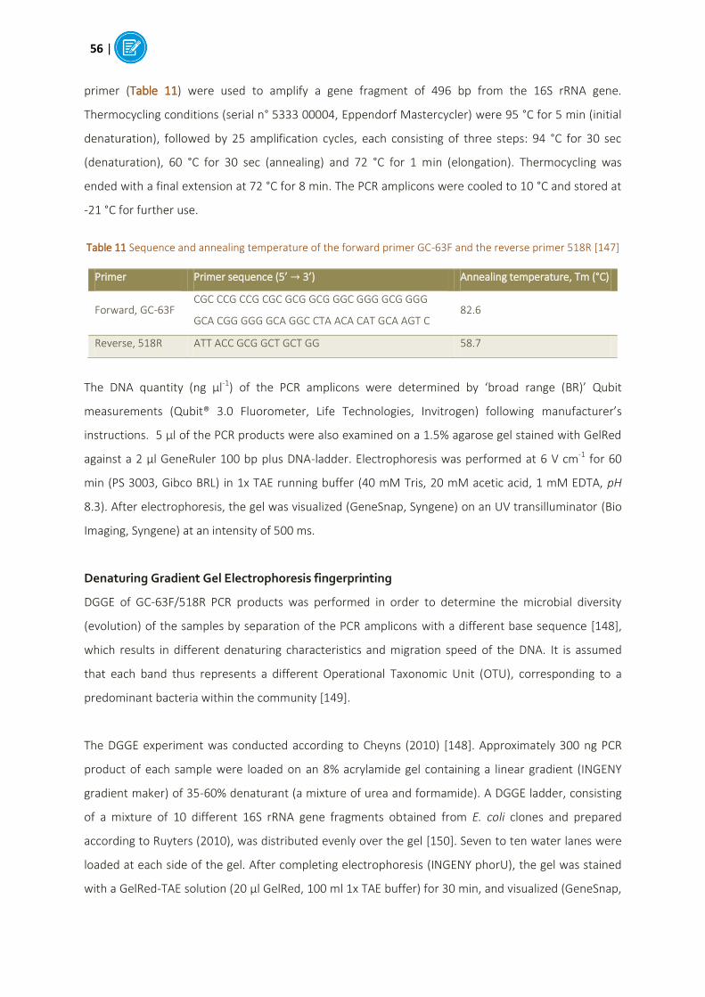
56 |

primer (Table 11) were used to amplify a gene fragment of 496 bp from the 16S rRNA gene.

Thermocycling conditions (serial n° 5333 00004, Eppendorf Mastercycler) were 95 °C for 5 min (initial

denaturation), followed by 25 amplification cycles, each consisting of three steps: 94 °C for 30 sec

(denaturation), 60 °C for 30 sec (annealing) and 72 °C for 1 min (elongation). Thermocycling was

ended with a final extension at 72 °C for 8 min. The PCR amplicons were cooled to 10 °C and stored at

-21 °C for further use.

Table 11 Sequence and annealing temperature of the forward primer GC-63F and the reverse primer 518R [147]

Primer Primer sequence (5’ 3’) Annealing temperature, Tm (°C)

Forward, GC-63F CGC CCG CCG CGC GCG GCG GGC GGG GCG GGG

GCA CGG GGG GCA GGC CTA ACA CAT GCA AGT C 82.6

Reverse, 518R ATT ACC GCG GCT GCT GG 58.7

The DNA quantity (ng µl-1) of the PCR amplicons were determined by ‘broad range (BR)’ Qubit

measurements (Qubit® 3.0 Fluorometer, Life Technologies, Invitrogen) following manufacturer’s

instructions. 5 µl of the PCR products were also examined on a 1.5% agarose gel stained with GelRed

against a 2 µl GeneRuler 100 bp plus DNA-ladder. Electrophoresis was performed at 6 V cm-1 for 60

min (PS 3003, Gibco BRL) in 1x TAE running buffer (40 mM Tris, 20 mM acetic acid, 1 mM EDTA, pH

8.3). After electrophoresis, the gel was visualized (GeneSnap, Syngene) on an UV transilluminator (Bio

Imaging, Syngene) at an intensity of 500 ms.

Denaturing Gradient Gel Electrophoresis fingerprinting

DGGE of GC-63F/518R PCR products was performed in order to determine the microbial diversity

(evolution) of the samples by separation of the PCR amplicons with a different base sequence [148],

which results in different denaturing characteristics and migration speed of the DNA. It is assumed

that each band thus represents a different Operational Taxonomic Unit (OTU), corresponding to a

predominant bacteria within the community [149].

The DGGE experiment was conducted according to Cheyns (2010) [148]. Approximately 300 ng PCR

product of each sample were loaded on an 8% acrylamide gel containing a linear gradient (INGENY

gradient maker) of 35-60% denaturant (a mixture of urea and formamide). A DGGE ladder, consisting

of a mixture of 10 different 16S rRNA gene fragments obtained from E. coli clones and prepared

according to Ruyters (2010), was distributed evenly over the gel [150]. Seven to ten water lanes were

loaded at each side of the gel. After completing electrophoresis (INGENY phorU), the gel was stained

with a GelRed-TAE solution (20 µl GelRed, 100 ml 1x TAE buffer) for 30 min, and visualized (GeneSnap,

| 57

Syngene) on an UV-transilluminator (Bio Imaging, Syngene) at an intensity of 400 ms. Community

fingerprint images were processed and analyzed with GelCompar ll software (Applied Maths) and a

dendrogram, calculated with the Dice coefficient taking into account the number of shared bands, was

constructed from clustering of all data from the gels based on the UPGMA32 algorithm. The structural

diversity of the samples was compared based on the Shannon diversity index evaluation of the

normalized band patterns of the specific groups, H, based on the underlying formula [149], [151]:

H = Equation 23

With S the number of species and Pi the relative frequency of the observations.

4.3. Physico-chemical analysis of the biofilm

At the end of Fouling Period 2, the fouled C-membranes were taken out of the bioreactor and the

biofilm structure (thickness, composition, density) was investigated by means of (microscopic) fouling

measurement techniques: ATR-FTIR, SEM and CLSM.


ATR-FTIR allows determination of the functional groups of organic membrane foulants [24]. Two

coupon replicates were carefully cut out of the fouled membranes taking care not to disturb or

destroy the biofilm. The coupons underwent the same procedure as described previously in this

chapter in Section 3.2.1.


Scanning Electron Microscopy (SEM) allows for qualitative description of the morphology of the

foulants [76]. Two coupon replicates were carefully cut out of the fouled membranes taking care not

to disturb or destroy the biofilm. The coupons did undergo a stringent pretreatment adapted from the

procedure described by Miura (2006) and Meng (2007) [76], [90]. The samples were first fixed by

immersion in 25 ml 3% (v/v) glutaraldehyde solution in 0.1 M phosphate buffer (pH 7.2) for 2 h. The

samples were then washed twice for 10 min followed by 1 h in 0.1 M phosphate buffer (pH 7.2).

Finally the samples were dehydrated in a seven-step ethanol series in mQ-H2O (25%, 50%, 75%, 85%,

95%, 100%, 100%) for 15 min each dehydration step. The dehydrated samples were mounted on a

SEM-holder by means of double-sided adhesive tape and coated prior to surface-analysis as described

32

Unweighted Pair Group Method of Arithmetic means

58 |

previously (Section 3.2.2). They were examined at an accelerating voltage of 25 kV and magnifications

250x, 1500x and 10 000x.

4.3.3. Confocal Laser Scanning Microscopy

Confocal Laser Scanning Microscopy (CLSM) is an optical microscope technique [152] which allows for

3D and depth visualization of the biofilm structure as well as determination of the biofilm thickness.

The biofilm is stained with dyes targeting the biopolymers of interest and the fluorescence light is

visualized. Moreover it may allow for discrimination of the membrane foulants (proteins, bacteria,

polysaccharides) and determination of their spatial distribution within the biofilm [24].

One coupon was carefully cut out of the fouled membranes taking care not to disturb or destroy the

biofilm. The coupon was immersed in 25 ml 0.1 M phosphate buffer and stored in the fridge during 24

h prior to staining and without additional fixation. The biofilm was stained based on the procedure

adapted from Lee et al. (2007) [106]. The samples were incubated at room temperature in the dark

during 30 min after immersion in a 10 ml mixture of 5 µM of two non-selective nucleic acid

fluorescence dyes in 10 mM MgSO4.7H2O, being SYTO 9 and SYTO 62, which are specific to

prokaryotes but may also stain eukaryotic microorganisms (cytoplasmatic, mitochondrial or nuclear

staining) [153]. Proteins and polysaccharides were not stained. The stained biofilm was fixed on a

microscope cover glass. The images were immediately acquired (Olympus Fluoview Viewer software,

Ver.4.1) with a laser-scanning microscope (FV1000-lX81, Olympus Fluoview) by means of the

objectives UPLanSAPO 40x/0.90 ∞0.17/FN26.5 (magnification 40x) and UPLanSAPO 100x/1.40oil

∞/0.17/FN26.5 (magnification 100x). At magnification 40x, depth images were acquired by optical

sectioning using steps of 1 µm, while at magnification 100x the step sizes were set at 0.5 or 0.25 µm.

Biofilm thicknesses were calculated by multiplying the number of slices taken by the size of each step.

The image size was adjusted to 512 x 512 pixels, 1x zoom and an aspect ratio 1:1. Signals were

recorded sequentially in the green channel (SYTO 9, excitation at 488 nm, emission at 500-524 nm)

and in the red channel (SYTO 62, excitation at 635 nm, emission at 655-755 nm). Finally the three

dimensional structure of the biofilm was reconstructed and images were processed (evaluation

version, Imaris Bitplane, Zurich, Switzerland).

5. STATISTICAL ANALYSIS

It is assumed that the variables follow a normal distribution (µ, σ2) with variance σ . The only

exception is the Shannon diversity index which is assumed to follow a lognormal distribution, since it is

| 59

calculated based on environmental samples [154]. Thus it is converted to log-values prior to analysis.

All data are expressed as (mean standard deviation s) with n the sample size or replicates.

Although statistical hypothesis testing between two small populations is not a very powerful tool,

independent two-tailed Student’s t-tests were applied to determine if two sets of data are significantly

different from each other based on a mutual comparison of all possible pairs of means µi [155].

Null hypothesis H0: µ1 = µ2 Equation 24 Alternative hypothesis Ha: µ1 µ2 Equation 25

t-statistic T =

Equation 26

With the pooled standard deviation sx1 x2 =

Equation 27

With the unbiased estimator of the variance of sample i. Reject H0 if |T| >

with α = 0.05 the

statistical significance, ʋ = 2n-2 the degrees of freedom and

from tables. Probability values (p-

values), indicating statistical significance, are also given. Sample means were considered significantly

different at a 95% confidence interval (p < 0.05).

| 61

Chapter 4: Results & discussion

The results obtained from the membrane physico-chemical related measurements (ATR-FTIR, SEM,

AFM, CAM, volume porosity measurement, electrokinetic characterization) and permeability related

measurements (CWP, critical flux) on the pure and functionalized PAN membranes, as well as

biofouling characterization measurements of the biofilm based on molecular techniques (PCR-DGGE)

and physico-chemical techniques (ATR-FTIR, SEM, CLSM), are presented here. Each section is

concluded with a brief summary, marked by ҉, meant for busy people. But first the stability of

operation of the HT-MBR is assessed.

1. MEMBRANE BIOREACTOR AND QUALITY MEASUREMENTS

The HT-MBR, which was operated at intermittent mode (8 min filtration – 2 min relaxation) and which

contained four replicates of each membrane type (i.e., the neutral membranes 13% PAN (neutral), the

negatively charged membranes 11% PAN-H (-) and 11% PAN-H, 2 layers (-) and the positively charged

membranes 11% PAN-H, 1 layer (+)), was monitored during both Transient Periods 1 and 2 and Fouling

Periods 1 and 2, which were defined in Section 2.1.3 of Chapter 3. Table 12 and Table 13 give an

overview of the operating conditions and physico-chemical properties of the HT-MBR respectively. For

an extensive discussion on the values presented here as well as microscopic investigation of the sludge

suspension, protamylasse feed solution and permeate, please refer to Section 1 of Appendix 1.

Table 12 Summary of the characteristics and operating parameters of the HT-MBR over both Transient Periods 1

and 2 and Fouling Periods 1 and 2. Values are given as (mean standard deviation).

Parameter Value Parameter Value

Reactor volume (l) 37.8 Total cross-flow rate (l day-1

) 25.6 3.1

Activated sludge volume (l) 20 Aeration rate (LPM) 10

Protamylasse feed solution

concentration (ml l-1

) 1.5 2.3

Dissolved oxygen concentration

(mg O2 l-1

) 4.6 0.6

HRT (hours) 18.75 SVI (ml g-1

) 153 37

SRT (days) 100 pH 7.81 0.24

TSS (g l-1

) 6.05 1.74 VSS (g l-1

) 5.31 1.79

Average volumetric loading rate (kg COD m

-3 d

-1)

1.05 Average sludge

loading rate (kg COD kg-1

TSS d-1

) 0.17

Temperature (°C) 13.6 1.2

62 |

Table 13 COD, TN and phosphate concentrations in the feed solution, the sludge supernatant and/or the permeate as well as their nutrient ratio and the removal efficiencies (%). Values are given as (mean standard

deviation). sCOD = soluble COD.

Parameter Feed solution Sludge Permeate Removal efficiency (%)

COD (mg O2 l-1

) 823.1 202.3 71.2 10.2 90.9 2.9

sCOD (mg O2 l-1

) 98.2 20.9

TN (mg TN l-1

) 132.8 39.5 70.7 33.1 49.3 22.9

P (mg PO43-

-P l-1

) 9.9 3.7 8.4 2.0 25.5 11.8

COD:N:P 100:17:1 100:138:18

҉ Summarized, the HT-MBR started to show steady-state behaviour at the end of Fouling Period 2.

The activated sludge pH provided the required membrane surface charges. The bioreactor exhibited

normal biomass concentrations with irregularly shaped flocs and good carbon, nitrogen and phosphate

removal efficiencies over the complete experimental period, but the activated sludge settled poorly due

to proliferation of filamentous bacteria. This might among others be due to an unevenly distributed

oxygen supply within the bioreactor. Moreover the sludge was inhabited by a series of non-bacterial

microorganisms. Thus overall the sludge was of good to moderate quality and the membranes seemed

to fully retain microorganisms from the sludge suspension.




Figure 24 gives the ATR-FTIR spectra of the P-membranes. The ATR-FTIR spectra of the C-membranes

are given in Section 2.1.1 of Appendix 1, together with the discussion. The absorbance values

correspond to typical literature values (from below 0.010 to 0.35), although most authors do not

indicate absorbance values or units on their graphs. The 13% PAN (neutral) membranes show three

important peaks at 1450 cm-1, 2240 cm-1 and 2935 cm-1, corresponding to the (-CH-) bend of PAN

backbone, the nitrile (C N) stretching vibration of the membrane surface groups and the asymmetric

(-CH-) stretching vibration of the PAN backbone, respectively [121], [126], [156].

The spectrum of the 11% PAN-H (-) membranes show the three same important peaks as the neutral

membrane type. The hydrolysis procedure did not transform all surface nitrile groups into carboxylate

groups since the peak at 2240 cm-1 did not change significantly. Additionally, a prominent peak at

1690 cm-1 can be noticed, corresponding to the carbonyl (-C=O) stretch vibration of the carboxylate

surface groups, as well as a peak at 3100 cm-1 corresponding to the carboxylate (O-H) stretch

vibration. For instance Moya et al. (2001), Moharram et al. (2002) and Kirwan et al. (2003) assigned

the carbonyl (-C=O) stretching vibration to FTIR-peaks in the range 1685-1725 cm-1 [156]–[158]. The

| 63

shifting to lower wavenumbers could be attributed to an interaction between the (-C=O) groups and

the nitrile (C N) groups remaining at the membrane surface after hydrolysis. As shown in Figure 15

(Chapter 3) amide groups (-CONH2) could be produced during the first hydrolysis step and be

subsequently transformed into carboxylate groups. However no amide group peak (1570 cm-1) [126]

was present on the FTIR spectra, thus indicating the predominance of the carboxylate groups and

complete hydrolysis.

Figure 24 ATR-FTIR spectra of the four membrane types (P-membranes).

The 11% PAN-H, 1 layer (+) and 11% PAN-H, 2 layers (-) membranes exhibit the same peaks as the 13%

PAN (neutral) and the 11% PAN-H (-) membranes. Indeed the application of one and two

polyelectrolyte layers respectively on the 11% PAN-H membrane, interrupted with rinsing steps, may

result in an incomplete coating of the membrane surface thus carboxylate and nitrile surface groups

can protrude into the external environment. Moreover the polymers are believed to undergo

interpenetration and rearrangement at the membrane surface in function of the pH of the solution,

thus being present at an equal volume fraction, independent on which polymer was deposited first

[159]. Additionally, the membranes exhibit a peak at 3350 cm-1, corresponding to the asymmetric

amine (N-H) stretch [158].

҉ Summarized, the ATR-FTIR results show the presence of the required functional groups on the

membrane surfaces which provide them with neutral (C N) or charged properties (-COO-, -NH3+) in

aqueous solutions or in the sludge suspension when these are characterized by a pH ranging between

the pKa values of the respective functional groups.

0

0,02

0,04

0,06

0,08

0 500 1000 1500 2000 2500 3000 3500 4000

Arb

itra

ry a

bso

rban

ce u

nit

s

Wavenumber (cm-1)

13% PAN, neutral 11% PAN-H (-) 11% PAN-H, 1 layer (+) 11% PAN-H, 2 layers (-)

1450 cm-1

-CH- bend

2240 cm-1

Nitrile C N stretch

1690 cm-1

Carboxylate –C=O stretch

3350 cm-1

Amine N-H stretch 2935 cm-1

-CH- stretch

3100 cm-1

Carboxylate O-H stretch

64 |


Figure 25 shows the surface and cross-sectional images of the four membrane types (P-membranes) at

different magnifications. The SEM cross-sectional and surface images of the C-membranes are given in

Section 2.1.2 of Appendix 1, together with the discussion.

The cross-sectional images (D) of Figure 25 show asymmetric integrally skinned membranes consisting

of finger-like pores or macrovoids extending from just below the membrane surface to the Novatexx

support over a distance of approximately 250 µm, corresponding to the wet casting thickness during

membrane manufacturing. This open porous structure developed after phase-inversion provides

physical support for the selective top layer at the membrane surface, which can be hardly

distinguished. The distance between the top layer and the top of the macrovoids, the so-called sub

layer, ranges between 1.4 and 2.1 µm for the 13% PAN (neutral) membrane and between 0.6 and 1.2

µm for the 11% PAN-H (-) as well as for the 11% PAN-H, 1 layer (+) and 11% PAN-H, 2 layers (-)

membranes (images (E) of Figure 25). As seen from the images (D) and (E), surface modification of the

PAN membrane (hydrolysis or/and coating) may adjust membrane properties but do not alter the

macroporous structure. The deposited PAH and PAA layers at the membrane surface cannot be

distinguished on the cross-sectional images (E) since their individual thickness must range between 3

and 5 Å at pH 6 (i.e., the pH of the rinsing solution during membrane synthesis) [159], [160]. Since

membrane preparation for SEM is a meticulous work, some errors can occur during membrane

fracturing, as has been the case for 11% PAN-H (-) (image (E) of Figure 25) where no clear cut was

obtained. It had been better to dip the membrane in liquid nitrogen before fracturation.

Next, the surface images (A) and (B) exhibit a relatively rough structure consisting of depressions of

approximately 600 nm diameter, which are apparently amplified as polyelectrolyte layers are coated

upon the membrane surface (compare 13% PAN (neutral) to 11% PAN-H, 2 layers (-), images (A), (B)

and (D) of Figure 25). Apparent increasing surface roughness with increasing number of deposited

layers has already been reported [125]. The depression-like structures may be confused with pores,

however these are not, nor artefacts due to sample preparation or to the SEM electron beamer, as

has been confirmed by AFM measurements (Section 2.1.3). Fritzsche et al. (1993) reported these

depression-like structures to be caused by small macrovoid structures residing between 90 and 200

nm below the membrane surface above the larger macrovoids and originating from the phase

inversion process (PAN concentration not mentioned) [44]. They may extend to the surface and cause

ruptures around which the membrane surface is depressed due to rapid water intrusion into the fluid-

like nascent membrane. However no such small macrovoids can be detected here on the cross-

sectional images (E). Yet most authors mostly do report smooth surfaces of the PAN and PAN-H

| 65

membranes instead of structural depressions (e.g., [123], [125], [126]), but the final membrane

morphology always is dependent on the coagulation bath temperature and the polymer

concentration: lower temperatures and higher polymer concentrations (and thus higher viscosity of

the casting solution) result in more dense and smooth surfaces [121], [122], [124].

Figure 25 SEM surface and cross-sectional visualization of the four membrane types (P-membranes). (A) 10 kV, magnification 1500x, (B) 10 kV, magnification 10 000x, (C) 12 kV, magnification 50 000x, (D) 10 kV, magnification

300x or 330x, (E) 10 kV, magnification 3000x.

Ding et al. (2015) investigated the surface structure of PAN membranes made of different PAN

concentrations and reported to distinguish pores at a 500x magnification for 8 wt% PAN membranes

in DMSO, but not at higher PAN concentrations (12 wt%, 16 wt%, 20 wt%, 24 wt%) [124]. However

here it is assumed that their designated pores might be artefacts of their membrane surface because

of their large size. The real pores are actually only visible at magnifications 50 000x or higher and are

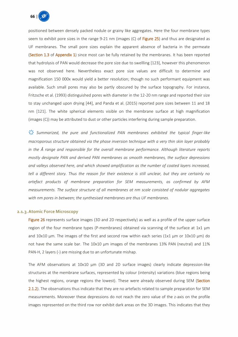
66 |

positioned between densely packed nodule or grainy like aggregates. Here the four membrane types

seem to exhibit pore sizes in the range 9-21 nm (images (C) of Figure 25) and thus are designated as

UF membranes. The small pore sizes explain the apparent absence of bacteria in the permeate

(Section 1.3 of Appendix 1) since most can be fully retained by the membranes. It has been reported

that hydrolysis of PAN would decrease the pore size due to swellling [123], however this phenomenon

was not observed here. Nevertheless exact pore size values are difficult to determine and

magnification 150 000x would yield a better resolution; though no such performant equipment was

available. Such small pores may also be partly obscured by the surface topography. For instance,

Fritzsche et al. (1993) distinguished pores with diameter in the 12-20 nm range and reported their size

to stay unchanged upon drying [44], and Panda et al. (2015) reported pore sizes between 11 and 18

nm [121]. The white spherical elements visible on the membrane surface at high magnification

(images (C)) may be attributed to dust or other particles interfering during sample preparation.

҉ Summarized, the pure and functionalized PAN membranes exhibited the typical finger-like

macroporous structure obtained via the phase inversion technique with a very thin skin layer probably

in the Å range and responsible for the overall membrane performance. Although literature reports

mostly designate PAN and derived PAN membranes as smooth membranes, the surface depressions

and valleys observed here, and which showed amplification as the number of coated layers increased,

tell a different story. Thus the reason for their existence is still unclear, but they are certainly no

artefact products of membrane preparation for SEM measurements, as confirmed by AFM

measurements. The surface structure of all membranes at nm scale consisted of nodular aggregates

with nm pores in between; the synthesised membranes are thus UF membranes.

2.1.3. Atomic Force Microscopy

Figure 26 represents surface images (3D and 2D respectively) as well as a profile of the upper surface

region of the four membrane types (P-membranes) obtained via scanning of the surface at 1x1 µm

and 10x10 µm. The images of the first and second row within each series (1x1 µm or 10x10 µm) do

not have the same scale bar. The 10x10 µm images of the membranes 13% PAN (neutral) and 11%

PAN-H, 2 layers (-) are missing due to an unfortunate mishap.

The AFM observations at 10x10 µm (3D and 2D surface images) clearly indicate depression-like

structures at the membrane surfaces, represented by colour (intensity) variations (blue regions being

the highest regions, orange regions the lowest). These were already observed during SEM (Section

2.1.2). The observations thus indicate that they are no artefacts related to sample preparation for SEM

measurements. Moreover these depressions do not reach the zero value of the z-axis on the profile

images represented on the third row nor exhibit dark areas on the 3D images. This indicates that they

| 67

are no pores, as already concluded earlier. These conclusions are assumed to be equally valid for the

13% PAN (neutral) and 11% PAN-H, 2 layers (-) membranes.

Figure 26 Atomic Force Microscopy observations (2D and 3D) of the four membrane types at 1x1 µm and of only two membrane types at 10x10 µm surface areas (P-membranes). The first and second row of images within each

series (1x1 µm or 10x10 µm) represent the three dimensional and the two dimensional surface structure respectively. The third row of images within each series represents the profile structure of the upper surface

region of the membranes.

The AFM images at 1x1 µm scale indicate the presence of assemblies of nodule-like structures on the

membrane surface and thus confirm the SEM observations. The actual pores are to be found between

these nodules and are represented as small dark areas. Since they are assumed to have a diameter

around 10-20 nm that does not shrink upon drying [44] they cannot be observed on the profile images

of the 1x1 µm images either. Though, the small profile segments extending to the zero-value of the z-

axis might possibly be considered as pores that are not fully detected due to forces interacting

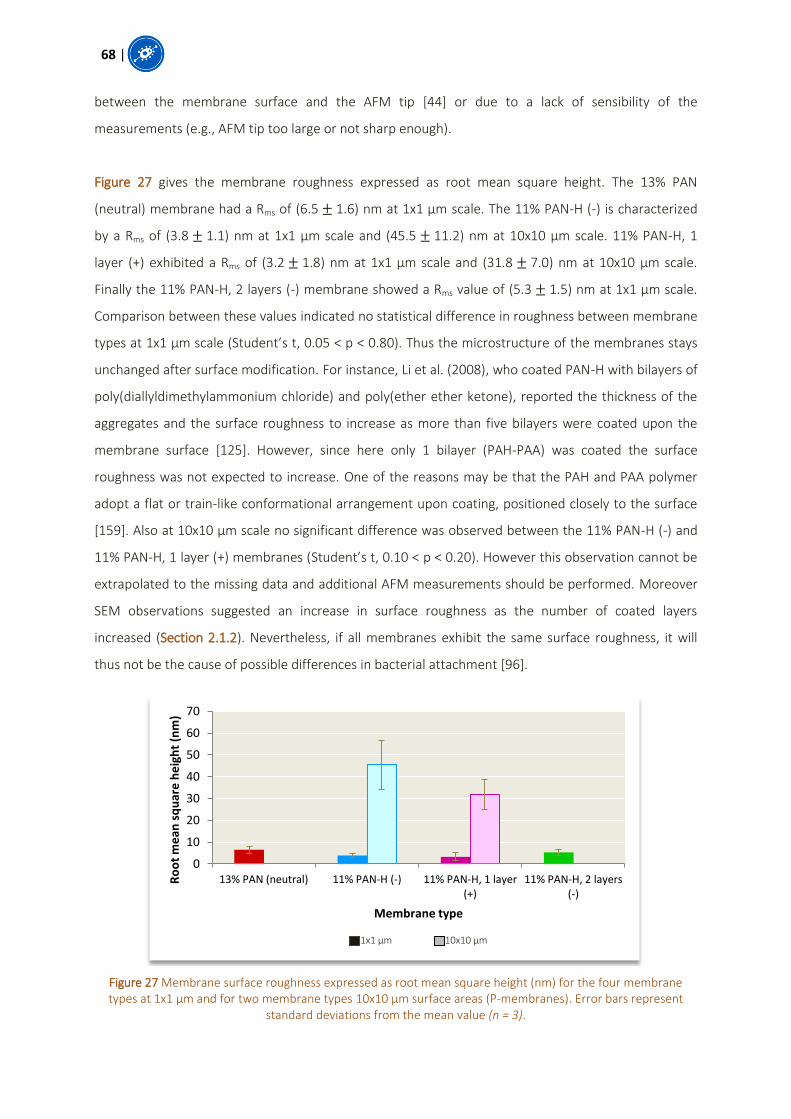
68 |

between the membrane surface and the AFM tip [44] or due to a lack of sensibility of the

measurements (e.g., AFM tip too large or not sharp enough).

Figure 27 gives the membrane roughness expressed as root mean square height. The 13% PAN

(neutral) membrane had a Rms of (6.5 1.6) nm at 1x1 µm scale. The 11% PAN-H (-) is characterized

by a Rms of (3.8 1.1) nm at 1x1 µm scale and (45.5 11.2) nm at 10x10 µm scale. 11% PAN-H, 1

layer (+) exhibited a Rms of (3.2 1.8) nm at 1x1 µm scale and (31.8 7.0) nm at 10x10 µm scale.

Finally the 11% PAN-H, 2 layers (-) membrane showed a Rms value of (5.3 1.5) nm at 1x1 µm scale.

Comparison between these values indicated no statistical difference in roughness between membrane

types at 1x1 µm scale (Student’s t, 0.05 < p < 0.80). Thus the microstructure of the membranes stays

unchanged after surface modification. For instance, Li et al. (2008), who coated PAN-H with bilayers of

poly(diallyldimethylammonium chloride) and poly(ether ether ketone), reported the thickness of the

aggregates and the surface roughness to increase as more than five bilayers were coated upon the

membrane surface [125]. However, since here only 1 bilayer (PAH-PAA) was coated the surface

roughness was not expected to increase. One of the reasons may be that the PAH and PAA polymer

adopt a flat or train-like conformational arrangement upon coating, positioned closely to the surface

[159]. Also at 10x10 µm scale no significant difference was observed between the 11% PAN-H (-) and

11% PAN-H, 1 layer (+) membranes (Student’s t, 0.10 < p < 0.20). However this observation cannot be

extrapolated to the missing data and additional AFM measurements should be performed. Moreover

SEM observations suggested an increase in surface roughness as the number of coated layers

increased (Section 2.1.2). Nevertheless, if all membranes exhibit the same surface roughness, it will

thus not be the cause of possible differences in bacterial attachment [96].

Figure 27 Membrane surface roughness expressed as root mean square height (nm) for the four membrane types at 1x1 µm and for two membrane types 10x10 µm surface areas (P-membranes). Error bars represent

standard deviations from the mean value (n = 3).

0

10

20

30

40

50

60

70

13% PAN (neutral) 11% PAN-H (-) 11% PAN-H, 1 layer (+)

11% PAN-H, 2 layers (-)

Ro

ot

me

an s

qu

are

he

igh

t (n

m)

Membrane type

1x1 µm 10x10 µm

| 69

҉ Summarized, AFM observations complement and confirm the SEM observations: the valleys

observed at the membrane surfaces are inherent structures of the membranes, while the effective

pores lie between nodular structures covering the surface at the nm scale. The membranes exhibited

the same roughness at 1x1 µm scale indicating that the microtopography of the pure PAN membrane

was not influenced upon modification and due to specific conformational arrangement of the coated

polymers. The observations at 10x10 µm scale cannot be extrapolated to the missing data, but there

might be an indication that the surface roughness is not significantly different either between

membranes at this scale.

2.1.4. Contact Angle Measurement

Figure 28 gives the contact angles ϑ of the four membrane types (P-membranes) measured with d-

H2O. The water drops were absorbed extremely fast by the dried membranes, indicating their

hydrophilic character and wettability (i.e., wetting angles values below 90 degrees).

Figure 28 Contact angle images of the four membrane types (P-membranes) performed with d-H2O, and their

respective contact angle ϑ. Values are given as (mean standard deviation) (n = 2 x 3).

As expected the pure PAN membrane (13% PAN (neutral)) showed to be more hydrophobic than the

charged membranes with an average contact angle of 69.8 degrees. Values in literature are reported

to vary between e.g., 47 degrees for 12 wt% PAN [124] to 76 degrees for 20 wt% PAN [121]. Ding et al.

(2015) reported the degree of hydrophilicity of PAN membranes to be dependent on polymer

concentration and phase inversion conditions [124]. They found that increasing polymer

concentrations and higher coagulation bath temperatures render a more polar membrane surface,

thus enhancing hydrophilicity.

70 |

The hydrolyzed PAN membrane (11% PAN-H (-)) showed increasing membrane wettability with an

average ϑ value of 18.4 degrees, due to the polar character of the carboxylate (-COO-) surface groups,

thus facilitating hydrogen bonding with the water molecules [110]. The pH of the d-H2O drop used

during the experiment was not measured, but it is assumed to be in the range 4.5-5.8 [161]. Indeed

freshly produced d-H2O should have a pH of 7 due to the lack of ions, but during use it comes into

contact with atmospheric carbon dioxide, thus reducing the pH to slightly acidic values. In this pH

range, the carboxylic surface groups were ionized for 80-90 % [159].

The difference in degree of hydrophilicity between the positively and negatively charged coated

membranes must be explained by a difference in charge of the PAN-H surface on the one hand and

the charge density of the polyelectrolytes on the other hand. It has been reported that the surface

wettability and thickness of weakly charged polyelectrolyte multilayers is strongly dependent on the

pH of the rinsing solution used during layer-by-layer deposition, since it controls the charge density of

the adsorbing polymers as well as the charge density of the previously adsorbed polymers [159].

However at pH 6 (i.e., the pH of the rinsing solution used here during the layer assembly), PAH is fully

protonated while PAA and the 11% PAH-H (-) membrane are almost fully protonated (80-90 %). In this

pH region, both PAH and PAA polymers are reported to be deposited as very thin layers of

approximately the same thickness (3-5 Å) due to spreading of the polymer chains over the surface

instead of stacking upon one another [159]. Moreover the polymers are believed to undergo

interpenetration and rearrangement at the membrane surface in function of the pH of the solution,

thus being present at an equal volume fraction, independent on which polymer was deposited first

[159]. Thus, although CAM theoretically only gives information on the degree of hydrophilicity of the

outer layer of the membrane surface [78], it may be assumed here that the results are slightly

influenced by the underlying charges (11% PAN-H (-) and/or 11% PAN-H, 1 layer (+)). These

conclusions are further strengthen by the observations made during the electrokinetic

characterization, explained later (Section 2.1.6).

In the pH range of the d-H2O drop used for the experiment (pH 4.5-5.8), the degree of ionization of

the carboxylic groups decreases (-COO- -COOH). This phenomenon is less pronounced for 11% PAN-

H, 2 layers (-) than for 11% PAN-H (-). For instance, a statistical comparison of the wetting angles of

both negatively charged membranes showed that the ϑ value of 11% PAN-H (-) is significantly different

from the ϑ value of 11% PAN-H, 2 layers (-) (Student’s t, p < 0.01), indicating that 11% PAN-H, 2 layers

(-) is more hydrophilic than 11% PAN-H (-). Indeed, it has been reported that assembly of

polyelectrolytes into a multilayered structure alters the dissociation constant (pKa) of the individual

polyelectrolytes compared to their value in aqueous solution due to the influence of local electrostatic

| 71

forces after coating [128]. Burke et al. (2003) explained this phenomenon by assuming that the

charged surface upon which the polyelectrolyte is coated, promotes protonation or dissociation of the

deposited layer to neutralize the residual negative or positive charges respectively, and does this more

strongly than repulsive forces between neighbouring groups resulting from this protonation or

dissociation [128]. For instance PAA would experience a shift to lower pKa values (pKa 4.5 4.1), i.e.,

an increase in acidic strength [128], while 11% PAN-H (-) does not, explaining the difference in contact

angle due to differences in degree of ionization of the surface charges.

In contrast to PAA, the amino groups of PAH stay fully protonated in the pH range of the d-H2O drop

used for the experiment (pH 4.5-5.8). But although the amount of PAA surface charges decreases

slightly at pH 4.5-5.8 compared to PAH, this change is assumed to be almost insignificant. Therefore

11% PAN-H, 2 layer (-) is assumed to have a larger charge density than 11% PAN-H, 1 layer (+) due to

its smaller atomic mass unit (compare 1.55E-25 Da for the monomer allylamine hydrochloride to

1.20E-25 Da for the monomer acrylic acid), thus explaining its more hydrophilic character. Indeed,

both polymers bear one charge per monomer.

҉ Summarized, the neutral pure 13% PAN membrane, characterized by chemically inert nitrile (C N)

surface groups, showed a higher degree of hydrophobicity than the functionalized charged PAN

membranes, of which the polar character was provided by the carboxylate (-COO-) and amine (-NH3+)

surface groups at the pH of the test-water. The negatively charged 11% PAN-H, 2 layers (-) seemed to

be the most hydrophilic membrane due to a shift in the dissociation constant of its surface carboxylate

groups upon coating on the one hand, as well as a charge density difference on the other hand. These

phenomena explain its larger hydrophilic character compared to hydrolyzed PAN and positively

charged PAN membrane, respectively. Overall, due to interpenetration phenomena of the coated

polymer layers, the CAM results are assumed to be slightly influenced by the charges of the underlying

structures, and these observations are strengthened by electrokinetic characterization of the

membranes. Thus based on the results presented here, it could be expected that the negatively charged

membranes, which show the largest hydrophilicity, would foul more slowly than the positively charged

membrane, and itself more slowly than the neutral PAN membrane, as explained previously in Chapter

3, Section 3.4.2. However, hydrophobicity is not the major parameter affecting fouling behaviour, as

seen in Section 2.2.2.

2.1.5. Volume porosity measurement

Figure 29 represents the volume porosity of the four membrane types (P-membranes). 13% PAN

(neutral) exhibits a volume porosity of (31.5 4.1) %. 11% PAN-H (-) exhibits a volume porosity of

72 |

(27.0 3.6) %. Finally 11% PAN-H, 1 layer (+) and 11% PAN-H, 2 layers (-) have a volume porosity of

(37.1 4.0) % and (36.5 7.0) % respectively. Statistical comparison of the measurements shows no

significant difference between the porosities of the membrane types (Student’s t, 0.10 < p < 0.80),

indicating that the surface modifications (hydrolysis, layer-by-layer deposition) did not alter the

porosity. However it has already been reported that higher polymer concentrations result in

membranes with a lower porosity [122], [124]. Thus it could have been expected that the 11 wt% PAN

membranes would have been more porous than the 13 wt% PAN membrane. The porosities are higher

than generally reported in literature for UF membranes (0.1-5% [38]). However Panda et al. (2015)

reported a porosity of 25% for a membrane made of 20% PAN [121]. Since high polymer

concentrations yield denser membranes, it can be assumed that the porosity values obtained here for

13 wt% and 11 wt% PAN membranes are accordingly reliable. High porosities yield high permeabilities,

as has been observed indeed (Section 2.2.1 of this chapter).

Figure 29 Membrane volume porosity measurements (-) of the four membrane types (P-membranes) based on water uptake measurements. Error bars represent standard deviations from the mean value (n = 2).

҉ Summarized, all membranes exhibited the same high volume porosity of around 30%, indicating

that surface modification by hydrolysis and layer-by-layer deposition did not alter the membrane

structure.

2.1.6. Electrokinetic characterization

Figure 30 represents the streaming current coefficient in function of the pH of the electrolyte solution

pumped tangential to the membrane surface of the four membrane types (P-membranes). The

membrane samples as well as the non-woven support did swell considerably during the

measurements and exhibited inconsistent results compared to expectations, as will be presented

0

25

50

75

100

13% PAN (neutral)

11% PAN-H, (-) 11% PAN-H, 1 layer (+)


Me

mb

ran

e v

olu

me

po

rosi

ty (

%)

Membrane type

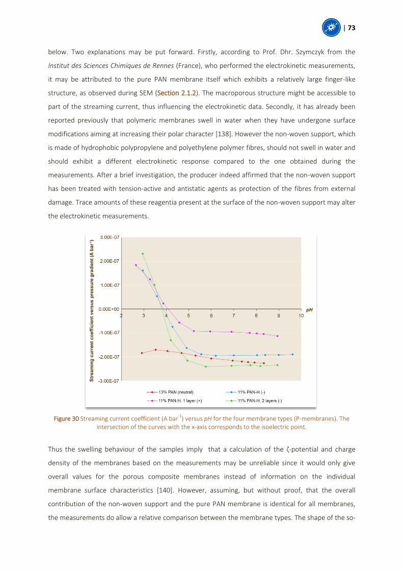
| 73

below. Two explanations may be put forward. Firstly, according to Prof. Dhr. Szymczyk from the

Institut des Sciences Chimiques de Rennes (France), who performed the electrokinetic measurements,

it may be attributed to the pure PAN membrane itself which exhibits a relatively large finger-like

structure, as observed during SEM (Section 2.1.2). The macroporous structure might be accessible to

part of the streaming current, thus influencing the electrokinetic data. Secondly, it has already been

reported previously that polymeric membranes swell in water when they have undergone surface

modifications aiming at increasing their polar character [138]. However the non-woven support, which

is made of hydrophobic polypropylene and polyethylene polymer fibres, should not swell in water and

should exhibit a different electrokinetic response compared to the one obtained during the

measurements. After a brief investigation, the producer indeed affirmed that the non-woven support

has been treated with tension-active and antistatic agents as protection of the fibres from external

damage. Trace amounts of these reagentia present at the surface of the non-woven support may alter

the electrokinetic measurements.

Figure 30 Streaming current coefficient (A bar-1

) versus pH for the four membrane types (P-membranes). The intersection of the curves with the x-axis corresponds to the isoelectric point.

Thus the swelling behaviour of the samples imply that a calculation of the ζ-potential and charge

density of the membranes based on the measurements may be unreliable since it would only give

overall values for the porous composite membranes instead of information on the individual

membrane surface characteristics [140]. However, assuming, but without proof, that the overall

contribution of the non-woven support and the pure PAN membrane is identical for all membranes,

the measurements do allow a relative comparison between the membrane types. The shape of the so-

74 |

called ‘acid-base titration curve’ [128] (i.e., plot of streaming current potential against pH) and the

position of the isoelectric point stay unchanged when plotting the ζ-potential, calculated from the

streaming current potential via the Helmholtz-Smoluchowski equation, against pH. If the non-woven

support has a large contribution to the streaming current data, it will also have a large contribution to

the derived ζ-potential values. Though, Prof. Dhr. Szymczyk is considering performing electrokinetic

measurements on the bare non-woven support as well as on free-standing membrane films in the

near future in order to clear up the research question. The remainder of this section thus attempts to

interpret the data collected so far.

As seen from Figure 30 the charged membranes (11% PAN-H (-) as well as 11% PAN-H, 1 layer (+) and

11%-PAN-H, 2 layers (-)) do exhibit a different behaviour compared to the neutral 13% PAN membrane

over the pH range considered, although all membranes show acidic behaviour [162].

The 13% PAN (neutral) membrane shows a stable negative charge independent on the pH of the

electrolyte solution and does not have an isoelectric point, i.e., the data points do not cross the x-axis

thus there is no pH where the ζ -potential is equal to zero [133]. Among other studies [126], [139], Cho

et al. (2012), who investigated the ζ-potential of nanofibres made of 11 wt% PAN in DMF as solvent at

a pH ranging between 5 and 8 and based on streaming current measurements, indicated almost

exactly the same behaviour but without providing substantial explanation [137]. According to Prof.

Dhr. Szymczyk, the observation made for the 13% PAN (neutral) membrane suggests the presence of

strong acid functions onto its surface and may be the result of interference with the non-woven PP/PE

support, since pure polyacrylonitrile is stable in aqueous solutions. However the studies mentioned

above do not report the use of such kind of non-woven support, thus the explanation might be

incomplete. A possible complementary explanation for the negative surface charges may also come

from Kolská et al. (2013). They stated that water molecules might undergo intensified autolysis (2 H2O

H3O+ + OH-) at the surface of (highly) hydrophobic membranes and the OH- molecules may adsorb

preferably to hydrophobic, non-polar or chemically inert surfaces compared to the H3O+ molecules. On

the contrary, the K+ and Cl- ions from the electrolyte solution are indifferent to these surfaces [138].

Moreover, rough surfaces, like of the PAN membranes (Section 2.1.2), have been reported to exhibit a

strong influence on the ζ-potential since the flow of the electrolyte solution over the membrane

surface is not evenly distributed and may result in higher surface charges [138].

In contradiction to 13% PAN (neutral), all charged membranes exhibited the same behaviour with an

isoelectric point around pH = 4 and thus indicating that they bear a positive net charge at a pH < 4 and

a negative net charge at a pH > 4. Here the charge mechanism is dominated by the ionization or

| 75

dissociation of the surface groups (‘intrinsic charges’ [126]) instead of preferential adsorption of ions

from the electrolyte solution [138]. According to Prof. Dhr. Szymczyk, the horizontal trend in the data

points from around pH = 5.5 suggests the presence of weak acid functions onto their surfaces, and

indeed, the surface carboxylic are reported to be weak acids [128]. On the contrary the surface amine

groups are weak bases, thus should exhibit a reversed S-shaped curve with a plateau at positive

streaming current potential. Several observations can be made.

Firstly, the inflection point of the curves has been reported to be the point where the pH equals the

dissociation constant (pKa) of the functional groups [128]. The trend represented by 11% PAN-H (-)

has already been observed by Bao et al. (2009), who investigated the electrokinetic behaviour of

hollow fibre hydrolyzed PAN membranes over the pH range 3-9 and in different electrolyte solutions

[126]. As expected, most of the carboxylic surface groups (dissociation constant pKa 5) are

negatively charged at a pH > pKa. However at low pH the membrane exhibits positive surface charges.

The K+ ions from the electrolyte solution probably to not adsorb on the membrane surface [138] thus

it cannot explain this increase in streaming current in acidic conditions. Bao et al. (2009) explain this

phenomenon by a shrinking of the carboxylic groups at low pH [126]. Moreover the electrokinetic

properties of 11% PAN-H (-) might possibly be explained by the contribution of residues from tension-

active and antistatic agents on the underlying hydrophilized non-woven support, which were possibly

not observable for the hydrophobic 13% PAN (neutral) membrane, thus leading to an overestimation

of the real electrokinetic values [140].

Secondly, the pKa value of the polymers PAH and PAA in solution are 8.7 and 4.5 respectively. Since

the results shown in Figure 30 indicate that their pKa in the multilayer structure is around pH = 4, it

seems to indicate a shift to lower apparent pKa values. The observation corresponds partly with the

ones made during the contact angle measurements (Section 2.1.4) and already reported by Burke et

al. (2003) [128]. The trend shown by 11% PAN-H, 1 layer (+) membrane, coated with PAH as polymer

layer, exhibits a reverse S-shaped curve compared to what has been reported in literature, as already

mentioned above [128]. However the overall trend still is as expected since the membrane is

positively charged at a pH below the apparent pKa value of the coated polymer. The negative values at

high pH might indicate the contribution of the hydrolyzed non-woven support and the PAN-H

underlying membrane structure to the overall surface charge: once all amine groups are deionised

(i.e., back to neutral state), the membrane becomes negatively charged due to deprotonation of the

carboxylate groups of the PAN-H structure [162]. Finally the pH-dependency of the 11% PAN-H, 2

layers (-) membrane is as expected [128] since these membranes bear carboxylate surface groups and

are thus negatively charged at a pH above the apparent pKa. The positive charges at low pH may

76 |

indicate a substantial contribution of the underlying PAH layer to the overall surface charge, based on

the same principle as mentioned above.

҉ Summarized, the extensive swelling of the macroporous structures of the synthesized composite

membranes (i.e., the chemically modified non-woven support as well as the pure PAN membrane),

indicating their accessibility to part of the streaming current, did alter the electrokinetic measurements

by providing data values only valid for the overall composite membranes. Subsequent derivation of the

zeta potential and surface charge densities was not possible. Nevertheless the raw streaming current

measurements suggest the presence of strong acid functions onto the surface of the neutral pure PAN

membrane, and of weak acid functions onto the surface of the charged membranes. Conclusions on the

pKa shift of coated layers drawn from the CAM measurements, might be confirmed here. However the

underlying structures may have a substantial contribution to these observations. Future electrokinetic

measurements on the bare non-woven support and the free-standing membrane films are planned in

order to complete the data and explain the measurements.


2.2.1. Clean water permeance

Figure 31 gives the clean water permeability of the four membrane types, for both the P- as well as the

C-membranes. The discussion on the permeability results of the C-membranes, as well as the

calculated hydraulic resistances (Rm) of the membranes are given in Section 2.2.1 of Appendix 1. The

permeabilities were not corrected to a standard temperature of 20 °C, but were all obtained by

filtration at room temperature (fluctuating around 21.6 °C).

Statistical comparison of the permeabilities obtained by filtration of the coupons and filtration of the

respective P-modules demonstrated that the CWP values of the coupons were not different from the

modules, as expected, except for the membrane 11% PAN-H (-), were a statistical difference was

obtained (Student’s t, 0.02 < p < 0.03). However the choice of the threshold significance limit is

arbitrary (here set at 95%). If a 99% confidence interval was chosen instead, no statistical difference

would have been noted. The permeability values of the P-membranes fluctuate around an overall

CWP value of 890 LMH bar-1. However most authors report pure water permeability values of around

210 LMH bar-1 for 16 wt% PAN [124] and 250 LMH bar-1 for 13 wt% PAN [122]. Thus the synthesised

membranes are characterised by high permeabilities decreasing the need for severe pumping and

reducing overall operational costs. Mutual statistical comparison of the coupons and the modules

indicated a significant difference between the CWP values of the 13% PAN (neutral) and 11% PAN-H, 2

| 77

layers (-) coupons and modules (Student’s t, 0.001 < p < 0.005 and 0.03 < p < 0.04 respectively). This

could be explained by the slight increase in membrane thickness upon layer-by-layer deposition, thus

slightly decreasing the clean water permeability [37]. Moreover the swelling behaviour of PAA in

contact with a solvent at pH 5-7 (here : mQ-H2O) has been reported to decrease the membrane

permeability [163].

Figure 31 Clean water permeance (LMH bar-1

) of coupons (pristine) (n = 3 x 3) and modules (P- and C-membranes) (n = 4 x 2) of the four membrane types, performed with mQ-H2O. Error bars represent standard

deviations from the mean value.

҉ Summarized, the membrane coupons and the respective membrane modules were characterized by

the same high clean water permeance of around 890 LMH bar-1. Thus together with the observations

and conclusions drawn from the physico-chemical related measurements (ATR-FTIR, SEM, AFM, CAM,

volume porosity measurement, electrokinetic characterization), the initial requirement is fulfilled,

namely to obtain neutral and charged membranes for which the fouling behaviour would be solely

determined by charge difference or membrane material and not by differences in pore size

(distribution), clean water permeability or surface roughness.

2.2.2. Critical flux

Figure 32 shows the flux-stepping experiment performed on the 13% PAN (neutral) modules (C-

membranes). Figure 33 shows the evolution of the mean fouling rate in function of the applied flux,

based on the measurements obtained during the flux-stepping experiment of the 13% PAN (neutral)

modules. As seen from the graph, the fouling rate increased exponentially during the flux-stepping

0

1000

2000

3000

4000

5000



Cle

an w

ate

r p

erm

ean

ce (

LMH

bar

-1)

Membrane coupons (P-membranes) Membrane modules (P-membranes)

Membrane modules (C-membranes)

78 |

experiment. The corresponding graphs for the cleaned 11% PAN-H (-), 11% PAN-H, 1 layer (+) and 11%

PAN-H, 2 layers (-) membranes are presented in Section 2.2.2 of Appendix 1. As the flux-stepping

experiment advanced, the TMP of the membranes did not decrease immediately back to 0 bar when

the permeate pump was interrupted at each flux-step, thus indicating that foulants gradually attached

to the membrane surface and could not be removed simply by flux stoppage but the aeration shear

forces had to interfere.

Figure 32 Flux-stepping measurements on 13% PAN (neutral) modules (C-membranes). Error bars represent

standard deviations from the mean value (n = 4).

Figure 33 Mean fouling rate (mbar h-1

) versus average flux (LMH) as determined in the flux-stepping experiment on 13% PAN (neutral) modules (C-membranes) (n = 4). The labels indicate the threshold limits for the critical flux

determination.

0

6

12

18

24

30

36

0

50

100

150

200

250

300

0 50 100 150 200 250 300

Flu

x sc

ale

(LM

H)

Tran

sme

mb

ran

e p

ress

ure

(m

bar

)

Time (min)

Transmembrane pressure Flux steps

-5,0 12,0

-50

0

50

100

150

200

250

300

350

0 10 20 30 40

Ave

rage

fo

ulin

g ra

te (

mb

ar h

-1)

Average flux (LMH)

Fouling rate

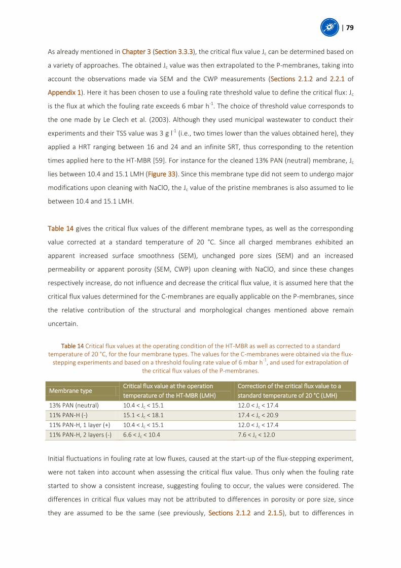
| 79

As already mentioned in Chapter 3 (Section 3.3.3), the critical flux value Jc can be determined based on

a variety of approaches. The obtained Jc value was then extrapolated to the P-membranes, taking into

account the observations made via SEM and the CWP measurements (Sections 2.1.2 and 2.2.1 of

Appendix 1). Here it has been chosen to use a fouling rate threshold value to define the critical flux: Jc

is the flux at which the fouling rate exceeds 6 mbar h-1. The choice of threshold value corresponds to

the one made by Le Clech et al. (2003). Although they used municipal wastewater to conduct their

experiments and their TSS value was 3 g l-1 (i.e., two times lower than the values obtained here), they

applied a HRT ranging between 16 and 24 and an infinite SRT, thus corresponding to the retention

times applied here to the HT-MBR [59]. For instance for the cleaned 13% PAN (neutral) membrane, Jc

lies between 10.4 and 15.1 LMH (Figure 33). Since this membrane type did not seem to undergo major

modifications upon cleaning with NaClO, the Jc value of the pristine membranes is also assumed to lie

between 10.4 and 15.1 LMH.

Table 14 gives the critical flux values of the different membrane types, as well as the corresponding

value corrected at a standard temperature of 20 °C. Since all charged membranes exhibited an

apparent increased surface smoothness (SEM), unchanged pore sizes (SEM) and an increased

permeability or apparent porosity (SEM, CWP) upon cleaning with NaClO, and since these changes

respectively increase, do not influence and decrease the critical flux value, it is assumed here that the

critical flux values determined for the C-membranes are equally applicable on the P-membranes, since

the relative contribution of the structural and morphological changes mentioned above remain

uncertain.

Table 14 Critical flux values at the operating condition of the HT-MBR as well as corrected to a standard

temperature of 20 °C, for the four membrane types. The values for the C-membranes were obtained via the flux-stepping experiments and based on a threshold fouling rate value of 6 mbar h

-1, and used for extrapolation of

the critical flux values of the P-membranes.

Membrane type Critical flux value at the operation

temperature of the HT-MBR (LMH)

Correction of the critical flux value to a

standard temperature of 20 °C (LMH)

13% PAN (neutral) 10.4 < Jc < 15.1 12.0 < Jc < 17.4

11% PAN-H (-) 15.1 < Jc < 18.1 17.4 < Jc < 20.9

11% PAN-H, 1 layer (+) 10.4 < Jc < 15.1 12.0 < Jc < 17.4

11% PAN-H, 2 layers (-) 6.6 < Jc < 10.4 7.6 < Jc < 12.0

Initial fluctuations in fouling rate at low fluxes, caused at the start-up of the flux-stepping experiment,

were not taken into account when assessing the critical flux value. Thus only when the fouling rate

started to show a consistent increase, suggesting fouling to occur, the values were considered. The

differences in critical flux values may not be attributed to differences in porosity or pore size, since

they are assumed to be the same (see previously, Sections 2.1.2 and 2.1.5), but to differences in

80 |

degree of hydrophilicity of the membranes. Madaeni et al. (1999) suggested that the Jc is larger for

more hydrophilic membranes [39]. It can be observed here that the more hydrophobic membranes

13% PAN (neutral) and 11% PAN-H, 1 layer (+) have low Jc values compared to the more hydrophilic

11% PAN-H membrane, as determined by contact angle measurements (see previously, Section 2.1.4).

However, as it was stated that 11% PAN-H, 2 layers (-) is the most hydrophilic membrane, it should

exhibit the larger critical flux. Since it is not the case here, it could be stated that although efforts have

been made to position the membrane replicates in the HT-MBR in such a way that they all experience

the same conditions, the 11% PAN-H, 2 layers (-) modules may have been subjected to lower aeration

shear forces than the other modules, thus increasing its initial fouling rate by rapid deposition of

sludge particles onto the membrane surface. However, eventually all membrane types exhibited the

same fouling rate, except 13% PAN (neutral) which seemed to have a larger fouling rate at high fluxes

(compare Figure 33 and A-Figure 11, A-Figure 13 and A-Figure 15 in Appendix 1).

҉ Summarized, the critical flux values of the membranes were influenced by the degree of

hydrophilicity of the membranes as well as positional aspects in the HT-MBR (uniformity of the oxygen

supply). Since the bioreactor was operated at 6.5 LMH, i.e., in sub-critical region for all membranes,

during both the Transient Periods and Fouling Periods, it thus can be concluded that no severe fouling

was expected to occur during long-term operation. Thus the gradual and slow fouling experiments

could be conducted without the need to clean the membranes chemically or to apply additional fouling

control strategies other than intermittent cross-flow operation with relaxation.



3.1.1. Bacterial enumeration

Figure 34 represents the dilution series in TSA performed on the sludge, protamylasse feed, permeate

and randomly chosen membrane samples. The sludge samples showed bacterial growth until dilution

10-5 (1 replicate) and 10-6 (2 replicates). The protamylasse feed samples taken at day 4 of the

maintenance period, exhibited growth until dilution 10-7 (2 replicates) and 10-8 (1 replicate). The

permeate samples showed growth until dilution 10-3 (1 replicate) and 10-4 (2 replicates). Finally the

randomly chosen membrane samples, which were actually two replicate modules of 13% PAN

(neutral) on Day 30 of the Fouling Period 2, showed growth until dilution 10-5 (2 replicate), 10-6 (3

replicates) and 10-7 (1 replicate).

| 81

Figure 34 Dilution series in Tryptone Soy Agar of the sludge, protamylasse feed (maintenance day 4), permeate and random two randomly chosen membranes (Day 30 of the Fouling Period 2) (n = 3).

Table 15 gives an estimate of the mean density of bacteria in the samples, expressed as Most Probable

Number (MPN) value per ml sample. The membrane samples were not expressed this way since the

sample was taken by scraping the membrane surface followed by resuspension in solution, thus the

original bacterial density cannot be expressed per ml or converted per surface area of the membrane.

In any case the membrane surfaces (i.e., pore channel fouling not taken into account) seemed to

exhibit a bacterial density as high as the sludge. For instance, Ivnitsky et al. (2007) reported that the

bacterial density on membranes are of the magnitude 106 colony-forming units (CFUs) cm-2, regardless

of the operating or hydrodynamic conditions of the MBR, the membrane type or the type of effluents

it treats [164].

Table 15 Approximate amount of bacteria in the sludge suspension, protamylasse feed solution from day 4 of the maintenance period, membrane surface and permeate, expressed as Most Probable Number (MPN) ml

-1 sample.

Sample MPN ml-1

Sludge 4.65 .107

Protamylasse feed solution 2.15 .109

Permeate 4.65 .105

The sludge seemed to house fewer bacteria than the protamylasse feed solution by a factor 100.

However three remarks can be made.

Firstly, the feed sample tested here is from day 4 of the maintenance period. As mentioned previously,

bacteria did develop in the feed tanks from the moment fresh feed was used until the moment the

feed was replaced. Thus the bacterial density found here is only a snapshot at a certain time point:

between day 1 and day 3, the density was less, between day 5 and day 8, the density was larger.

Secondly, the sludge was sonicated before inoculation in order to break the sludge flocs and disperse

bacteria as much as possible in the medium (compare the sludge structure in A-Figure 5 of Appendix 1

82 |

and in Figure 35 after sonication). Microscopic analysis performed after the treatment showed well-

dispersed cells and a decrease or even disappearance of filaments. There was no guarantee the

bacteria did not die during sonication or were fully dispersed and randomly distributed within the

sample after treatment. For instance it has been reported that the cell viability after sonication

reaches 55% [165]. If a certain amount of bacteria was still clumped or if a numerable amount of

bacteria died, the MPN value underestimates the actual bacterial density of the sludge. In this case, it

is probably better to speak of an estimation of the CFUs instead of the amount of individual bacteria

[142].

Figure 35 Microscopic image of the sludge sample after sonication (magnification 1000x, oil objective).

Finally, as has already been mentioned previously in Chapter 3, only 1-15% of all bacteria present in

activated sludge and introduced on laboratory media, are estimated to be cultivable [144], [145]. For

instance, since TSA is a very rich medium, slow growing bacteria are outcompeted by rapid growers.

Thus it could be estimated that the MPN value given here for the sludge must be multiplied by a factor

up to 100 in order to obtain the real amount of cells in the samples. No such derivation has to be

made for the permeate and the protamylasse feed samples, though. Indeed, it would be highly

unlikely that enormous amounts of bacteria are present in the permeate. Indeed, the bacteria are

retained by the membranes in the HT-MBR, as explained previously from the microscopic analysis

(Section 1.3 of Appendix 1), and although no special attention has been drawn to keep the permeation

tubes sterile (explaining the presence of bacteria), such high amounts of bacteria are not believed to

be able to grow in nutrient deficient conditions (i.e., the bacteria in the bioreactor process the

nutrients into new biomass). As for the synthetic feed solution, which is supposed to be free of

bacterial contamination upon inoculation, it can be viewed as a sort of laboratory medium left under

non-sterile conditions during the maintenance period. The high nutrient concentrations thus will

enhance rapid bacterial development.

҉ Summarized, based on the MPN technique, the activated sludge suspension seemed to house fewer

bacteria than the protamylasse feed solution by a factor 100. Among others, the effect of sonication

pretreatment on the cell viability as well as the low cultivability of bacterial members of natural

| 83

samples may be possible explanations. The high number of bacteria detected in the protamylasse feed

solution and the permeate are attributed to the non-sterile working conditions.


Figure 36 represents the evolution of the TMP of the replicate modules of 13% PAN (neutral)

immersed in the HT-MBR during Fouling Period 1. The equivalent graphs for the other membrane

types are presented in Section 3.1.1 of Appendix 1. As seen from Figure 36, the four membrane

replicates did not foul at the same rate. The main explanation for this phenomenon is the badly

distributed aeration of the HT-MBR, although a previous study [131] stated that positional effects for

this particular reactor are minimal. While the replicates 3 and 4 experienced shear forces along their

surfaces, replicates 1 and 2 were positioned in less turbulent zones thus the fouling layer could build

up. However the replicates show large variations in their TMP trend. Thus it is assumed that the

aeration conditions were quite variable even within the low-turbulence zone of the reactor. Also the

effect of membrane sampling and subsequent removal of a small amount of biofilm material may

explain the large variations within the TMP trend. The same trend can be observed in A-Figure 16, A-

Figure 17 and A-Figure 18 in Appendix 1. Thus the two module replicates of each membrane type

exhibiting the slowest fouling rate (e.g., module replicates 3 and 4 for 13% PAN (neutral) in Figure 36)

were used for culture-independent biofouling community characterization (see later, Section 3.2.1).

The other replicates were only used to keep the HT-MBR operated. The remainder of the discussion

deals with the slow fouling membrane replicates.

Figure 36 Evolution of the transmembrane pressure (mbar) of the module replicates of 13% PAN (neutral) during Fouling Period 1. Arrows indicate time points of biofilm sampling.

As seen on the Figures, the short-term ‘conditioning stage’ (Section 3.3 of Chapter 3) cannot be

distinguished since the TMPs were recorded on a daily basis instead of every hour of the first day of

0

100

200

300

400

500

600

700

17-nov. 27-nov. 07-déc. 17-déc. 27-déc. 06-janv.

Tran

sme

mb

ran

e p

ress

ure

(m

bar

)

Date Replicate 1 Replicate 2

Replicate 3 Replicate 4

84 |

immersion. The time-evolution of the TMP was characterized by a slow and linear rise (the

‘sustainable stage’), instead of a two-stage TMP profile often reported in literature, characterised by a

sudden TMP rise [99] [7]. Indeed, this sudden TMP rise occurs when membranes are already highly

fouled or in supra-critical conditions, but here the HT-MBR was operated at a flux below the critical

flux of the sludge suspension (Section 2.2.2), explaining the low TMP increment with time. All pairs of

membrane replicates seemed to foul at the same rate (0.32 mbar day-1 on average), with the

exception of 11% PAN-H, 2 layers (-) which exhibited a larger fouling rate (1.5 mbar day-1 on average).

Since the membrane modules were positioned the same way during the critical flux experiment

(Section 2.2.2) as during the whole Fouling Periods, the conclusion drawn from the critical flux

experiment can be extended here: although efforts have been made to position the membrane

replicates in the HT-MBR in such a way that they all experience the same conditions, the 11% PAN-H, 2

layers (-) modules may have been subjected to lower aeration shear forces than the other modules.

Visual inspection of the biofilm layer in development on the membrane surfaces did not reveal major

differences in structure, colour (brownish and relatively slimy) or coverage. However in the last week

of Fouling Period 1, before the pump malfunctions did occur, several dark brown and disperse pustule

or mushroom like structures developed on the membrane surface in a non-ordered way.

Unfortunately no picture or sample has been taken of these structures, thus it can only be speculated

that they may be of bacterial origin and may have originated from an intensively developing colony

present in the surface biofilm or newly attached to the membrane surface.

҉ Summarized, because of lack of uniformity in the aeration system of the HT-MBR, only two of the

four module replicates per membrane type were used to characterize the biofilm structure and

community composition. The chosen module replicates did foul linearly at an average fouling rate of

0.32 mbar day-1 and visually exhibited identical biofilms.


3.2.1. DGGE fingerprinting of PCR-amplified 16S rRNA gene fragments

The DNA quantity of the sludge, membrane and feed samples obtained by means of Qubit

measurements after PCR is presented in A-Table 2 and A-Table 3 of Appendix 1. The AGE gel obtained

after electrophoresis of the PCR products is presented in A-Figure 19 of Appendix 1, together with the

designation of the lanes in A-Table 4 and A-Table 5.

Figure 37 represents the dendrogram constructed from the 16S rRNA gene community fingerprint of

the membrane biofilms, the activated sludge and the protamylasse feed samples. Although numerous

| 85

intensive bands are distinguishable, representing the most dominant bacteria in the samples, some

weak bands result in a smear unfit for analysis. Most of the sequences exhibited a similarity at the

nodes of less than 90% (i.e., less than 90% of shared bands). Figure 38 gives the number of

Operational Taxonomic Units (OTUs) computed from the fingerprints of the four membrane types at

every sample time point. Although it is assumed that each band in the fingerprint corresponds to a

different OTU, some bacterial species could have the same G+C DNA content but a different base

sequence, thus a single band could represent different species [148], [151]. Moreover one bacterial

species could be represented by different fingerprints G+C sequence micro-heterogeneity and thus

produce multiple bands [143], [151], [166]. Thus the number of OTUs only gives an approximation of

the number and abundance of bacterial species within the community. Finally it must be said that

PCR-DGGE is reported to only detect bacterial populations that make up at least 1% of the total

community, thus bacterial populations present in very low abundance within the community are

mostly excluded from the analysis [143], [149], [151].

Firstly, based on Figure 37 it may be stated that the planktonic community of activated sludge differs

significantly from that of the protamylasse feed, and both differ significantly from the sessile

community of the membrane biofilms, independently on the sampling time point or on the membrane

type. Among other publications [89], [91], Huang et al. (2008) and Piasecka et al. (2012) already

observed that most of the OTUs detected in planktonic biomass were not detected in the biofilm

fingerprints [3], [6], or at least not in the same relative abundance [90]. While the α-, β-, γ- and δ-

Proteobacteria are the dominant species found in biofilms, as mentioned previously in Chapter 2

(Section 3.2.3), the activated sludge communities of both aerobic and anaerobic MBRs were reported

to be dominated by α-, β- or γ-Proteobacteria [6], [13], [64], [144], [145], [151] (e.g., Pseudomonas sp.

which is reported to always be present in activated sludge [13], [14]), Bacteroidetes [6], [64] and

Gram-positive bacteria characterized by a high G+C DNA content (generally > 50%) [145] (although

some members have found to be low G+C [167]). The latter include the class of the Actinobacteria and

more specifically the filamentous actinomycetes [8], [151], [168], to which M. parvicella, a filamentous

bacteria predominant in sludge and already presented previously in Section 1.3 of Appendix 1, is

related [28], [169]. However, since most of these bacteria have not been reported to colonize

membrane surfaces, it explains the band clustering of the dendrogram. Moreover the sludge profiles

exhibit small fluctuations over time during the fouling experiment (e.g., variation in relative abundance

of common bands). It has already been reported that planktonic bacterial community function and

structure in the sludge suspension are highly diverse but do fluctuate over time according the changes

in conditions of the HT-MBR [3], [6], [64]. On the contrary the protamylasse feed solutions did not

86 |

Figure 37 Bacterial 16S rRNA gene community fingerprints (DGGE profile showing differences in community structure and respective dendrogram) derived from membrane biofilms, activated sludge and protamylasse feed solution at different sampling time points of the Fouling Period 1 performed in the HT-MBR. The scale bar represents the

percentage similarity at the nodes. The standard markers were removed from the DGGE profile for the sake of clarity.

| 87

undergo physical or chemical changes between day 1 and day 8 of each of the maintenance periods,

allowing for a stable community to develop from day 1. A seen from Figure 37, the protamylasse feed

sample of day 1 of the maintenance period differs significantly from the feed samples of the other

days of the maintenance period, indicating it did not contain enough biomass as already supported by

microscopic investigation (Section 1.3 in Appendix 1). Finally the feed pellet developing at the bottom

of the feed tank exhibited a lower microbial abundance and diversity than the feed samples taken

from the solution.

Secondly the results reveal that the bacterial community of the membranes sampled on the first

sampling time point (25th of November 2014, Day 72) differs significantly from the bacterial

community of the membranes sampled at the other time points. The main reason might be that

membrane sampling did not yield enough bacterial DNA product for analysis since the pristine

membranes were only freshly immersed in the HT-MBR. Low DNA concentrations thus make it difficult

to perform fingerprint comparison analysis. For instance, the number of OTUs of the samples from 25-

Nov14 differed significantly from the number of OTUs of the other membrane sample time points

(Student’s t, 0.001 < p < 0.015) (Figure 38). On the other hand, since fingerprint analysis did indicate

the presence of a few fingerprint bands, it may indicate the development of a specific pioneer flora of

on average 20 pioneering OTUs during the very first hours and days of biofilm development on the

membrane surfaces that was eventually replaced by a different community later on. Piasecka et al.

(2012) already reported the presence of 25 OTUs responsible for pioneering biofilm development in a

MBR operated on molasses wastewater [6]. Only a specific set of species are known to be able to

initiate biofouling and to eventually modify the surface characteristics of the membrane resulting in

subsequent uniform fouling [6]. To cite two example studies, Zhang et al. (2006) found among others

the α-Proteobacteria to be the major bacterial populations present in biofilms of just a few hours old

[89], while Zhang et al. (2007) designated Acinetobacter calcoaceticus from the γ-subgroup of the

Proteobacteria to be a good biofouling initiator [170]. Since these bacterial populations also are

assumed to be some of the major populations in the sludge community (see above), it may be stated

that the dominant bacteria from the sludge initiate biofouling, but are eventually competed out in

mature biofilms, as already reported previously [6], [16], [171]. Indeed, the activated sludge

suspension may favour some dominant bacterial species, while bacteria present in low abundances

within the solution may grow preferably in nascent biofilms on the membranes due to e.g., protection

from fluctuations in living conditions [171], thus becoming selectively enriched in biofilms [171].

However according to Zhang et al. (2006) specific bacteria rather than the bulk biomass of the sludge

suspension are responsible for biofilm initiation [89].

88 |

Figure 38 Number of Operational Taxonomic Units derived from the number of band in the fingerprints of the membrane samples taken at different time points. Error bars represent standard deviations from the mean value

based on the band number of the four membrane types (n = 4).

Next, the lack of branch similarity between membrane types on the 25th of November 2014 (since they

do not cluster together) may indicate the influence of positional effects in the HT-MBR. For instance,

oxygen deficiency that was likely to occur in the sludge suspension surrounding membrane 11% PAN-

H, 2 layers (-) as already mentioned previously, could have modified the adhesion tendency of the

microbial species [24]. The lack of branch similarity may indicate membrane surface effects (here:

charge) as well in the selection of appropriate foulants. As explained previously in Chapter 2 (Section

3.4.2) 13% PAN (neutral) could have exhibited a lower fouling degree and biofilm diversity than 11%

PAN, 1 layer (+) [96], and itself could have had a lower fouling tendency than the 11% PAN-H (-) and

11% PAN-H, 2 layers (-) membranes [117], due to the influence of the surface charge. However the

surface effect would eventually fade out as the initial stages of fouling are surpassed due to deposition

and accumulation of material which covers the membrane surface. Overall, it would have been

interesting to perform a DGGE analysis on the two different membrane module replicates of the 25th

of November 2014 instead of merging the replicate DNA samples before PCR. Additionally alternative

fingerprinting techniques could be applied. A frequently used molecular technique is Terminal

Restriction Length Polymorphism (T-RFLP) fingerprinting [6], [13], [14], [64], [171], [172], which is

based on enzymatic digestion of fluorescently labelled PCR amplicons [173]. In combination with real-

time quantitative Polymerase Chain Reaction (qPCR), which allows for enumeration of the amplified

DNA extracted from the samples from both viable and death cells, and 16S rRNA gene-clone library

construction and sequencing, it would allow for visualization of the OTUs responsible for biofouling

initiation as well as for determination of the diversity and composition of the sludge and biofilm

communities. This might have allowed visualization of differences in pioneering bacterial communities

during the initial fouling stages, as to confirm above mentioned hypothesis statistically.

Finally, the results reveal that the bacterial community developing on the membranes differ between

sampling time points but not between membrane types. This suggests that the relative abundance

and structure of bacterial population changes with time due to interactions between members of the

0

10

20

30

40

50

25-Nov14 (Day 72)

01-Dec14 (Day 78)

08-Dec14 (Day 85)

15-Dec14 (Day 92)

19-Dec14 (Day 96)

02-Jan15 (Day 110)

Nu

mb

er

of

OTU

s

| 89

biofilm as well as with the external environment (e.g., fluctuating operating conditions and

hydrodynamics). These interactions modify the local biofilm environment with time by creating

ecological protective niches within the biofilm based on physical gradients, leading to exclusion or

favouring of existing members within the community [171]. β-Proteobacteria, or more specifically

Rhodocyclus- or Ralstonia-related bacteria, were reported to be the dominant phylogenetic group in

mature biofilms, although the relative dominance of the α-, β-, γ- and δ-Proteobacteria in biofilms may

vary with time due to e.g., variations in mixed liquor viscosity or aeration rate [90]. For instance it has

been reported that nutrient rich environments favour the γ-Proteobacteria against the β-subgroup

[90]. Martiny (2003), who examined the development of biofilms in a drinking water system during

three years, found that the biofilm communities did stabilize only after two years of operation [171].

However the fingerprints did not indicate an increase in bacterial species since no significant increase

in OTUs was observed throughout the sample time points (Student’s t, 0.10 < p < 0.80) (Figure 38).

Moreover the observation suggests that although there might be a selective attachment of bacteria

during the initial stages of fouling, the local characteristics of the membrane (here: charge) do not play

a decisive role on the long term in selecting the key foulants. Nevertheless one could consider

repeating the fouling experiment and using several HT-MBRs, each containing one membrane under

the same operating conditions, instead of using a single HT-MBR containing all 16 modules. This would

give guarantee that the MBR environment itself and the proximity of and thus possible mutual

interaction between the modules did not play a significant role in the long-term selection of key

foulants.

Figure 39 Log-values of the Shannon diversity index for the membrane and activated sludge samples. Error bars represent standard deviations from the mean value calculated from the values homogenized over the different

time points (n = 6).

A comparison of the log-values of the Shannon diversity indices of the membrane, feed and sludge

samples in Figure 39 indicate a statistical difference between the diversity of the membranes 13% PAN

(neutral) and 11% PAN-H (-) compared to membrane 11% PAN-H, 2 layers (-) (Student’s t, 0.001 < p <

0.005), while no statistical difference was found between 11% PAN-H, 1 layer (+) and 11% PAN-H, 2

layers (-) (Student’s t, 0.30 < p < 0.80). As already mentioned previously in Sections 2.2.2 and 3.1.2, the

0,00

0,25

0,50

0,75

1,00



activated sludge

Shan

no

n d

ive

rsit

y in

de

x

90 |

modules 11% PAN-H, 2 layers (-) may have been subjected to different aeration and turbulence

conditions in the HT-MBR, resulting in a shift in the microbial community structure and diversity

compared to other membrane types. According to expectations, the diversity of 11% PAN-H, 1 layer

(+) should also differ significantly from the diversity of 11% PAN-H, 2 layers (-). However, probably

because of the lack of bacterial DNA product yield from sampling, the banding patterns of 11% PAN-H,

1 layer (+) exhibited large differences in intensity compared to other membrane types (see the bands

on the 8th and 15th of December 2014 in Figure 37), thus rendering fingerprint analysis relatively

unreliable. Finally a comparison between the log-values of the Shannon diversity indices of the

membranes and the sludge samples revealed a significant higher diversity for the membrane samples

(Student’s t, p < 0.001), except for 11% PAN-H, 1 layer (+) (Student’s t, 0.1 < p < 0.2). This

inconsistency may be explained as done above. The observation is in contradiction with studies

reported earlier [89] where the planktonic biomass exhibited a higher diversity than the biofilm

community, but may be explained by a selective enrichment of specific bacterial species in the biofilm

compared to the bulk biomass. Moreover these bacterial populations may make up less than 1% of

the sludge community, thus remaining undetected by PCR-DGGE fingerprinting techniques. However,

since all publications used here to support the observations, report the application of different

operating conditions and the use of different membrane materials and wastewater types,

generalizations are very difficult to make. As reported by Boon et al. (2002), the Shannon diversity

index is only an indication of the diversity within a community rather than an absolute value [151].

҉ Summarized, since the planktonic communities of the activated sludge did exhibit differentiated

branching in the dendrogram from the sessile communities of the biofilm, independently on the

sampling time point or on the membrane type, it may be concluded that bacterial populations from the

sludge suspension were selectively enriched within the biofilms. Dominant bacteria from the sludge

may initiate biofouling, but are assumed to be eventually competed out in mature biofilms due to

physical and chemical changes of the local biofilm environment. Moreover, the membrane samples

exhibited a higher microbial diversity than the sludge samples at every time. Secondly variations in

biofilm community structure and composition were monitored over time, suggesting that local

variations in the biofilm and the gradual development of ecological protective niches favour or exclude

specific bacterial populations. The largest time-dependent difference in amount of OTUs was observed

between the samples from the first sampling time point (25-Nov14, Day 72) and the samples taken at

the other time points, most probably explained by a lack of bacterial product suitable for analysis.

Finally, the bacterial communities did not differ between membrane types at a certain sampling time

point, suggesting that the membrane surface charges do not affect biofilm community composition.

Although results tended to indicate small membrane surface effects on pioneering communities on the

| 91

first day of immersion, the major explanation probably has to be found in the influence of positional

effects within the HT-MBR, such as aeration issues. Thus, the local characteristics of the membrane

(here: charge) do not play a decisive role on the long term in selecting the key foulants. However the

experiment should be repeated with several HT-MBRs, each containing one membrane under the same

operating conditions, instead of using a single HT-MBR containing all 16 modules, in order to confirm

this hypothesis indisputably by excluding proximity effects. Moreover alternative and widely used

molecular techniques, such as a combination of T-RFLP, qPCR and 16S rRNA clone library construction

and sequencing, could be tested against PCR-DGGE fingerprint outcomes.

3.3. Physico-chemical analysis of the biofilm

As already explained in Section 2.2.1 of Appendix 1, the fouling experiment during Fouling Period 2 was

only performed on the cleaned 13% PAN (neutral) modules, since the other membrane types lost their

structural and chemical properties due to extended cleaning with NaClO. At the end of Fouling Period

2 (Day 190) the fouled modules were removed from the HT-MBR and the biofilm structure was

analysed using ATR-FTIR, SEM, AFM and CLSM.


ATR-FTIR was performed in order to identify the main components of the biomass developing on the

membrane surface. Figure 40 represents the ATR-FTIR spectrum of the membrane foulants of 13%

PAN (neutral) after a fouling period of 39 days, which differs considerably from the spectrum obtained

of the pristine membrane (Figure 24).

The only two peaks that are still visible from Figure 24 are the (-CH-) bend and stretch vibrations, at

wavenumbers 1450 cm-1 and 2930 cm-1 respectively [76], [130], which could be attributed to the PAN

backbone as well as to the carbon backbone of the biopolymers. The nitrile (C N) functional group of

the membrane material cannot be discerned anymore, suggesting the biofilm did cover the

membrane surface well. However, since only a small surface area of the membrane was screened, it

cannot be generalized to the whole surface coverage.

Proteins can be discerned from the peaks around 1530 cm-1 and 1630 cm-1 which are specific for the

secondary conformation of proteins, called Amide ll (N-H bend and C-N stretch) and Amide l (C=O

stretch) respectively [24], [76], [130], [174]–[176]. Meng et al. (2010) reported that the peak at 1630

cm-1 could also be attributed to aromatic compounds or humic-like substances [24]. Additionally the

peak around 1400 cm-1 corresponds to the asymmetric stretch of carboxyl (-COO-) or carbonyl (C=O)

groups of amino acids [24], [176]. The hydroxyl (O-H) stretch is represented by the broad peak at 3270

92 |

cm-1 [76]. However 3270 cm-1 could also be attributed to the (N-H) stretch vibration of proteins [174].

The peak around 1035 cm-1 may represent (C-O) stretch vibration of polysaccharides or

polysaccharide-like substances [76], [175], [176]. Finally the peak around 1230 cm-1 can be assigned

to the phosphate vibrations in nucleotides [175].

Figure 40 ATR-FTIR graph of the fouling layer of membrane 13% PAN (neutral).

Small shifts in wavenumber values or band intensities compared to those reported in literature may

be caused by differences in pH and ionic strength of the sludge, leading to conformational changes of

the biopolymers [24] or by the presence of other substituents on the biomolecules [176]. All

functional groups distinguished here suggest the presence of bacteria, protein and polysaccharide like

substances (biopolymers, humic substances) in the cake layer, mostly originating directly from

deposition of activated sludge material [130], and increase the degree of hydrophilicity of the biofilm ,

as already have been reported by Tansel et al. (2008) [98]. However Jinhua et al. (2006) reported that

the degree of hydrophobicity of bacteria may even increase when attached onto the membrane, thus

counterbalancing the relative increase in hydrophilicity of the biofilm and enhancing further bacterial

attachment [24], [91].

҉ Summarized, the spectrum of the fouled membrane differs considerably from the spectrum of the

pristine membrane and exhibits IR peaks mainly associated with bacteria (phosphate in nucleotides)

and biopolymers (proteins, polysaccharides).

0

0,02

0,04

0,06

0,08

0 500 1000 1500 2000 2500 3000 3500 4000

Arb

itra

ry a

bso

rban

ce u

nit

s

Wavenumber (cm-1)

13% PAN (neutral)

1530 cm-1

amide ll 1630 cm-1

amide l

1400 cm-1

amino acid –COO-

or C=O stretch

1035 cm-1

C-O stretch

2930 cm-1

-CH- stretch

3270 cm-1

hydroxyl O-H stretch

or protein N-H stretch 1450 cm-1

-CH- bend

1230 cm-1

nucleotides

| 93


SEM was performed in order to visualize the morphology of the biofilm and determine the

composition of the biofilm. Figure 41 shows the rough three dimensional structure of the biofilm

developing on the surface of the 13% PAN (neutral) membrane after 39 days of fouling. A comparison

of image (B) of Figure 41 with image (A) of Figure 25 indicates that the biofilm and deposited particles

covers the membrane surface well since the surface features of the pristine membrane cannot be

discerned anymore. Moreover the images show a clear size difference between the components of

the biofilm (µm range) and the depressions and pores (nm range) of the pristine membrane,

illustrating why the membranes were capable of retaining particulate matter and bacterial species

from the sludge suspension and the biofilm. A number of spherical and rod-shaped bioparticles (e.g.,

Bacillus sp.) as well as a network of filaments could be distinguished, embedded in a matrix of what it

is assumed to be biopolymers (EPS) or an artefact of SEM preparation (see for instance the viscous-like

structure surrounding the chains of rods in image (C) of Figure 41). Although SEM gives information on

the biofilm structure and allows for discrimination based on size and shape of the particles, it only

gives little information on the nature of the foulants (organic, inorganic) or on the specific bacterial

species. Moreover the rather stringent SEM pretreatment may alter the original structure of the

fouling layer [24]. Nevertheless SEM provides enjoyable images of the biofilm.

Figure 41 SEM surface images of the fouling layer of membrane 13% PAN (neutral) at magnifications 250x (A), 1500x (B) and 10 000x (C) and 25 kV.

҉ Summarized, the SEM images of the fouled membrane differ considerably from the SEM images of

the pristine membrane. The three-dimensional rough structure of the biofilm, consisting of organic and

inorganic material and embedded in a polymeric matrix, covers the membrane surface completely.

3.3.3. Confocal Laser Scanning Microscopy

Figure 42 represents the three dimensional architecture of the biofilm developing on the membrane

surface of 13% PAN (neutral) after 39 days of operation and at different magnifications. It also gives

access to a Youtube video highlighting the three dimensional composition of the fouling layer by

migration of the fluorescence signal over the cake depth, apparently without signal distortions or loss

94 |

of fluorescence with depth. The images are represented in green, since for any undetermined reason

staining and visualisation with SYTO 62 failed. The apparent loose coverage of the biofilm at

magnification 40x (image A) may be due to background subtraction in order to eliminate background

noise. Background subtraction was also applied on image B, but since the image was taken at another

location of the biofilm, the effect seems to be less pronounced.

The biofilm was approximately 45 µm in height dependent on the location on the membrane surface.

It has been reported that the biofilm thickness does not depend on the operating conditions of the

MBR, but tend to converge to the same order of magnitude, influenced by the balance between

nutrient level, shear forces and transmembrane pressure [3], [164]. The bottom of the biofilm is

uneven since the membrane surface was not smooth either (Sections 2.1.2 and 2.1.3) (the membrane

surface is not visible since it was not stained).

Figure 42 CLSM images of the biofouling layer of membrane 13% PAN (neutral) at magnifications 40x and 320x320 µm surface area (A) and magnification 100x and 125x125 µm surface area (B). The QR code

33 (C) gives

access to a Youtube video highlighting the three dimensional structure of the biofilm (100x) by migration of the fluorescence signal over the cake depth. The images and the video were processed by means of the software

evaluation version of Imaris Bitplane.

The biofilm was dense and mainly composed of discrete clusters of apparently a few dominant

bacteria on different locations and at different heights spread across the membrane surface, as can be

clearly seen in the video (QR code in Figure 42). The apparent low diversity may be in contradiction

with the fingerprinting results which suggested a highly diverse biofilm. Since the samples were not

fixated prior the CLSM analysis, a considerable amount of biofilm material may have been lost.

However, the discrete bacterial clusters may be characteristic to biofilms in development since mature

biofilms have been reported to consist of an even and smooth community structure without patches

of independent populations [171]. Thus it suggests that each cluster or colony developed from one

bacteria initially attaching onto the membrane surface or that bacteria seek each other and preferably

assemble instead of living as simple individual elsewhere in the biofilm. Indeed, microorganisms can

33

http://youtu.be/96bUH84PImM

http://youtu.be/96bUH84PImM

| 95

congregate by mutual detection and self-coordination based on the transfer of quorum sensing

molecules, a small signal molecule called an autoinducer [24]. This molecule accumulates in the

external environment when several bacterial members of the same species are present. When a

certain threshold value is reached, which is proportional to a certain cell density, the autoinducer

activates the transcription of specific genes, e.g., expressing surface adhesion proteins or excretion of

EPS [6], [104], resulting in species with sessile phenotypes that are strongly different from their

planktonic phenotypes [95]. For instance, it has been reported that the biofilm former Pseudomonas

aeruginosa, a member of the γ-Proteobacteria, is strongly capable of cell density dependent gene

regulation (e.g., in view of protection, transport, metabolism) [8], [95].

Image A (320x320 µm) and B (125x125 µm) of Figure 42 depict the presence of an extended network

of filamentous structures penetrating the biofilm with clearly visible septa between separate cells,

possibly being filamentous fungi while the more tiny filaments somewhat detectable on image B and

in de video might be of bacterial origin. Filamentous fungi, such as Aspergillus sp., have been reported

to be capable of biofilm formation, as well as EPS production [177] and quorum sensing (e.g., related

to sporulation) [178], although their biofilm formation mechanism differs slightly from biofilm

initiation and development by bacteria [178]. But since they were only observed very sporadically in

the activated sludge suspension by microscopic analysis (Section 1.3 of Appendix 1) it is rather

unexpected to observe them in the biofilm. On the contrary, to my knowledge filamentous bacteria

have not been reported to grow on membranes operated in an activated sludge suspension. The

presence of bacterial filaments in biofilms has only been reported in applications where no

membranes are used. For instance articles dealing with e.g., microbial fuel cells [179] and

ultracompact biofilm reactors [180], used for the generation of electric power from organic matter

and the treatment of wastewater respectively. They mentioned that the local conditions near the

biofilm, such as low pH values, low DO concentration or low surface loading rates initiate filamentous

overgrowth, and that once the filaments attach to the biofilm, further biofilm development is

inhibited. Thus, although these observations do not apply to MBR membranes, there is no direct

reason not to extend them to this specific environment.

҉ Summarized, the biofilm formed on the surface of the neutral pure PAN membrane had an average

thickness of 45 µm and was mainly composed of discrete clusters of bacteria, probably established via

quorum sensing mechanisms and evolving towards a smooth mature biofilm community. Moreover an

interpenetrating network of filamentous fungi and bacteria was observed, probably indicating some pH

or other deviations from normal operation near the biofilm surface.

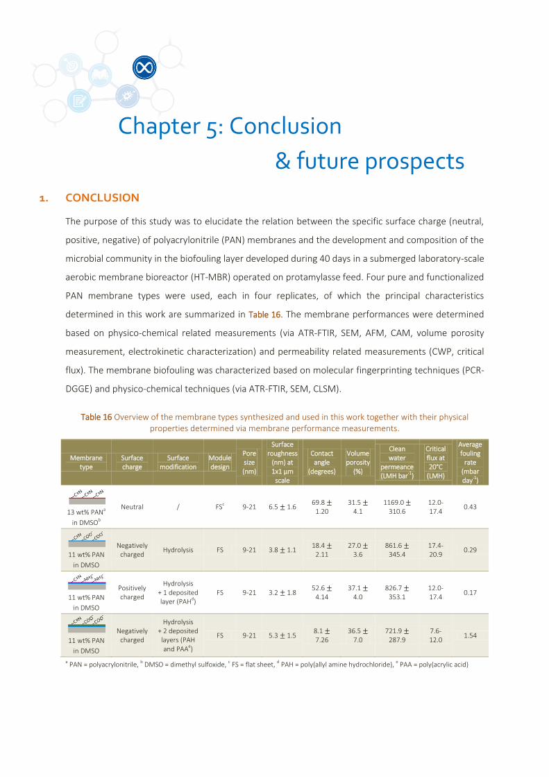
| 97

Chapter 5: Conclusion

& future prospects

1. CONCLUSION

The purpose of this study was to elucidate the relation between the specific surface charge (neutral,

positive, negative) of polyacrylonitrile (PAN) membranes and the development and composition of the

microbial community in the biofouling layer developed during 40 days in a submerged laboratory-scale

aerobic membrane bioreactor (HT-MBR) operated on protamylasse feed. Four pure and functionalized

PAN membrane types were used, each in four replicates, of which the principal characteristics

determined in this work are summarized in Table 16. The membrane performances were determined

based on physico-chemical related measurements (via ATR-FTIR, SEM, AFM, CAM, volume porosity

measurement, electrokinetic characterization) and permeability related measurements (CWP, critical

flux). The membrane biofouling was characterized based on molecular fingerprinting techniques (PCR-

DGGE) and physico-chemical techniques (via ATR-FTIR, SEM, CLSM).

Table 16 Overview of the membrane types synthesized and used in this work together with their physical properties determined via membrane performance measurements.

Membrane type

Surface charge

Surface modification

Module design

Pore size (nm)

Surface roughness

(nm) at 1x1 µm

scale

Contact angle

(degrees)

Volume porosity

(%)

Clean water

permeance (LMH bar-1)

Critical flux at 20°C

(LMH)

Average fouling

rate (mbar day-1)

13 wt% PANa

in DMSOb

Neutral / FSc 9-21 6.5 1.6 69.8

1.20 31.5

4.1 1169.0

310.6 12.0-17.4

0.43

11 wt% PAN

in DMSO

Negatively charged

Hydrolysis FS 9-21 3.8 1.1 18.4

2.11 27.0

3.6 861.6

345.4 17.4-20.9

0.29

11 wt% PAN

in DMSO

Positively charged

Hydrolysis + 1 deposited layer (PAHd)

FS 9-21 3.2 1.8 52.6

4.14 37.1

4.0 826.7

353.1 12.0-17.4

0.17

11 wt% PAN

in DMSO

Negatively charged

Hydrolysis + 2 deposited layers (PAH and PAAe)

FS 9-21 5.3 1.5 8.1 7.26

36.5 7.0

721.9 287.9

7.6-12.0

1.54

a PAN = polyacrylonitrile, b DMSO = dimethyl sulfoxide, c FS = flat sheet, d PAH = poly(allyl amine hydrochloride), e PAA = poly(acrylic acid)

98 |

The HT-MBR started to show steady-state behaviour at the end of the overall experimental period.

The bioreactor exhibited normal biomass concentrations with irregularly shaped flocs and good

carbon, nitrogen and phosphate removal efficiencies over the complete experimental period, but the

activated sludge settled poorly due to proliferation of filamentous bacteria. This might among others

be due to an unevenly distributed oxygen supply within the bioreactor. Moreover the sludge was

inhabited by a series of non-bacterial microorganisms. Thus overall the sludge was of good to

moderate quality and the membranes seemed to fully retain microorganisms from the sludge

suspension.

Membrane physico-chemical related measurements revealed the presence of the required functional

groups on the membrane surfaces (ATR-FTIR). They provided the membranes with neutral (C N) or

charged properties (-COO-, -NH3+) at the pH of the activated sludge suspension. SEM measurements

revealed typical finger-like macroporous structure with a very thin skin layer probably in the Å range

and responsible for the overall membrane performance. The surface depressions and valleys

observed at the surface of the membranes are certainly no artefact products of membrane

preparation for SEM measurements, as confirmed by AFM measurements. The surface structure of all

membranes at nm scale consisted of nodular aggregates with nm pores in between; the synthesised

membranes are thus UF membranes. No apparent difference in surface roughness was observed

between membrane types. CAM measurements indicated that the neutral pure 13% PAN showed a

higher degree of hydrophobicity than the functionalized charged PAN membranes. The negatively

charged 11% PAN-H, 2 layers (-) seemed to be the most hydrophilic membrane due to a shift in the

dissociation constant of its surface carboxylate groups upon coating on the one hand, as well as a

charge density difference on the other hand. Interpenetration phenomena of the coated polymer

layers resulted in an influence of the charges of the underlying structures on the CAM and streaming

current measurements. All membranes exhibited the same high volume porosity of around 30%,

indicating that surface modification by hydrolysis and layer-by-layer deposition did not alter the

membrane structure.

Permeability related measurements indicated that the membranes were characterized by a high clean

water permeance of around 890 LMH bar-1. Thus together with the observations and conclusions

drawn from the physico-chemical related measurements (ATR-FTIR, SEM, AFM, CAM, volume porosity

measurement, electrokinetic characterization), the initial requirement has been fulfilled, namely to

obtain neutral and charged membranes for which the fouling behaviour would be solely determined

by charge difference and membrane material and not by differences in pore size (distribution), clean

water permeability or surface roughness. Since the HT-MBR was operated at a flux below the critical

flux of the sludge suspension, the gradual and slow fouling experiments (average fouling rate 0.32

| 99

mbar day-1) could be conducted without the need to clean the membranes chemically or to apply

additional fouling control strategies other than intermittent cross-flow operation with relaxation.

PCR-DGGE fingerprinting revealed that the planktonic communities of the activated sludge did exhibit

differentiated branching in the dendrogram from the sessile communities of the biofilm,

independently on the sampling time point or on the membrane type. Thus it may be concluded that

bacterial populations from the sludge suspension were selectively enriched within the biofilms.

Moreover, the membrane samples exhibited a higher microbial diversity than the sludge samples at

every time. Secondly variations in biofilm community structure and composition were monitored over

time, suggesting that local variations in the biofilm and the gradual development of ecological

protective niches favour or exclude specific bacterial populations. The largest time-dependent

difference in amount of OTUs was observed between the samples from the first sampling time point

(25-Nov14, Day 72) and the samples taken at the other time points, most probably explained by a lack

of bacterial product suitable for analysis. Finally, the bacterial communities did not differ between

membrane types at a certain sampling time point, suggesting that the membrane surface charges do

not affect biofilm community composition. Although results tended to indicate small membrane

surface effects on pioneering communities on the first day of immersion, the major explanation

probably has to be found in the influence of positional effects within the HT-MBR, such as aeration

issues. Thus, the local characteristics of the membrane (here: charge) do not play a decisive role on

the long term selection of the key foulants.

Morphological visualization and chemical analysis of the 40 days old biofilm grown on the 13% PAN

(neutral) membranes revealed the presence of bacteria (phosphate in nucleotides) and biopolymers

(proteins, polysaccharides) (ATR-FTIR) and the 45 µm thick biofouling coverage consisted of discrete

bacterial clusters embedded in a polymeric matrix and interpenetrating by filamentous fungi and

bacteria (SEM, CLSM).

2. FUTURE PROSPECTS

Overall, following guideline may be taken into consideration in view of future work and data

validation. Enhanced knowledge of the specific relation between membrane and microorganisms as

well as inter-microbial relations, would allow for development of more targeted anti-fouling

strategies.

The experiment should be repeated with one HT-MBR for each membrane under the same

operating conditions, instead of using one single reactor containing all clusters, in order to exclude

100 |

proximity effects. Testing different feed solutions (of municipal, industrial origin), application of

alternative operating conditions (including sterile equipment) and synthesis of membranes with

different polymers and solvents might allow further process optimization in view of undisputable

validation of the observations over a wide range of applications. However the step further to

extrapolation to full-scale applications may still be a matter of uncertainty.

Membrane characterization of PAN membranes could be brought one step further by detailed

investigation of the surface microtopography and surface chemistry via optimization of techniques

that were not able to deliver reliable results here or not easily accessible, namely electrokinetic

measurements (for: surface charge density), porosimetry measurements (for: pore size

distribution, surface porosity and average pore size), Transmission Electron Microscopy (for: pore

size and surface topography), elemental analysis (for: chemical constituents), titration (for: ion-

exchange capacity).

Identification of the pioneering species as well as the relative contribution of the bacteria from the

activated sludge to biofilm formation, could complete the data. Three approaches could be used.

Firstly, the use of alternative and widely used molecular techniques such as a combination of T-

RFLP, qPCR and 16S rRNA clone library construction followed by Sanger sequencing, could be

tested against PCR-DGGE fingerprint outcomes and serve this purpose. Next, optimized use of the

CLSM techniques and Fluorescence In Situ Hybridization would allow for time-dependent

morphological characterization of the biofilm formers. Finally the application of cultivation-

dependent techniques including isolation from the sludge and biofilm samples on adequate

laboratory media followed by spiking of the activated sludge with selected and labelled members

of the pure cultures, would allow for further morphological and physiological characterization and

determination of the proportion of that specific member in the whole biofilm community.

A - I

References [1] N. Abdel-Raouf, a a Al-Homaidan, and I. B. M. Ibraheem, “Microalgae and wastewater treatment.,” Saudi

J. Biol. Sci., vol. 19, pp. 257–275, Jul. 2012.

[2] P. Grelier, S. Rosenberger, and A. Tazi-Pain, “Influence of sludge retention time on membrane bioreactor hydraulic performance.,” Desalination, vol. 192, pp. 10–17, May 2006.

[3] L.-N. Huang, H. De Wever, and L. Diels, “Diverse and Distinct Bacterial Communities Induced Biofilm Fouling in Membrane Bioreactors Operated under Different Conditions.,” Environ. Sci. Technol., vol. 42, pp. 8360–8366, Nov. 2008.

[4] S. Judd, “The status of membrane bioreactor technology.,” Trends Biotechnol., vol. 26, pp. 109–116, Feb. 2008.

[5] P. Le-Clech, “Membrane bioreactors and their uses in wastewater treatments.,” Appl. Microbiol. Biotechnol., vol. 88, pp. 1253–1260, 2010.

[6] A. Piasecka, C. Souffreau, K. Vandepitte, L. Vanysacker, R. M. Bilad, T. De Bie, B. Hellemans, L. De Meester, X. Yan, P. Declerck, and I. F. J. Vankelecom, “Analysis of the microbial community structure in a membrane bioreactor during initial stages of filtration.,” Biofouling, vol. 28, pp. 225–38, Jan. 2012.

[7] J. Zhang, H. C. Chua, J. Zhou, and A. G. Fane, “Factors affecting the membrane performance in submerged membrane bioreactors.,” J. Memb. Sci., vol. 284, pp. 54–66, Nov. 2006.

[8] M. Madigan, J. Martinko, D. Stahl, and D. Clark, Brock. Biology of Microorganisms., 13th ed. San Fransisco: Pearson Education, p. 1150.

[9] B. Van der Bruggen, “Cursustekst - I0S80A Waste Water Treatment Technology. Part 1: Legislation in Flanders and Primary Waste Water Technology.,” Acco, Acco - Leuven. 3rd edition., 2012.

[10] P. M. Armenante, “Characterization of Industrial Wastewaters.”

[11] I. Smets, “Cursustekst - I0S80A Waterzuivering en -hergebruik. Deel 2: Secundaire afvalwaterzuiveringstechnieken.,” Acco, Acco Leuven. 4th edition., 2012.

[12] D. Springael, “Cursustekst - I0N96A Milieutechnische Microbiologie.,” Katholieke Universiteit Leuven, Leuven, 2012.

[13] H. Waheed, I. Hashmi, A. K. Naveed, and S. J. Khan, “Molecular detection of microbial community in a nitrifying–denitrifying activated sludge system.,” Int. Biodeterior. Biodegradation, vol. 85, pp. 527–532, Nov. 2013.

[14] S. J. Khan, F. Parveen, A. Ahmad, I. Hashmi, and N. Hankins, “Performance evaluation and bacterial characterization of membrane bioreactors.,” Bioresour. Technol., vol. 141, pp. 2–7, Aug. 2013.

[15] “Titel ll van het VLAREM Bijlagen. Bijlagen bij het besluit van de Vlaamse Regering van 1 juni 1995 houdende algemene en sectorale bepalingen inzake milieuhygiëne.,” Departement Leefmilieu, Natuur en Energie, 1998. [Online]. Available: http://www.lne.be/themas/vergunningen/bestand/regelgeving/titel-ii-van-het-vlarem-bijlagen-pdf/view?searchterm=milieuhygiëne. [Accessed: 03-Jan-2015].

[16] L. Vanysacker, B. Boerjan, P. Declerck, and I. F. J. Vankelecom, “Biofouling ecology as a means to better understand membrane biofouling.,” Appl. Microbiol. Biotechnol., vol. 98, pp. 8047–72, Oct. 2014.

[17] E. Vaiopoulou, P. Melidis, and A. Aivasidis, “An activated sludge treatment plant for integrated removal of carbon, nitrogen and phosphorus.,” Desalination, vol. 211, pp. 192–199, Jun. 2007.

[18] S. Milia, G. Cappai, M. Perra, and A. Carucci, “Biological treatment of nitrogen-rich refinery wastewater by partial nitritation (SHARON) process.,” Environ. Technol., vol. 33, no. 13, pp. 1477–1483, 2012.

[19] Y. Peng and G. Zhu, “Biological nitrogen removal with nitrification and denitrification via nitrite pathway.,” Appl. Microbiol. Biotechnol., vol. 73, pp. 15–26, Nov. 2006.

[20] B. Kartal, J. G. Kuenen, and M. C. M. van Loosdrecht, “Sewage Treatment with Anammox.,” Science (80-. )., vol. 328, pp. 702–703, 2010.

A - II

[21] L. Zhang, P. Zheng, C. Tang, and R. Jin, “Anaerobic ammonium oxidation for treatment of ammonium-rich wastewaters.,” J. Zhejiang Univ. Sci. B, vol. 9, no. 5, pp. 416–426, May 2008.

[22] P. Xinhong, Y. Hongbing, W. Libo, A. Lina, and F. Lixia, “CANON Process for Nitrogen Removal from Effluents of Municipal Sewage Treatment Plants.,” Trans. Tianjin Univ., vol. 19, no. 4, pp. 255–259, 2013.

[23] K. A. Third, A. O. Sliekers, J. G. Kuenen, and M. S. M. Jetten, “The CANON System ( Completely Autotrophic Nitrogen-removal Over Nitrite ) under Ammonium Limitation : Interaction and Competition between three groups of Bacteria.,” Syst. Appl. Microbiol., vol. 24, pp. 588–596, 2001.

[24] F. Meng, B. Liao, S. Liang, F. Yang, H. Zhang, and L. Song, “Morphological visualization, componential characterization and microbiological identification of membrane fouling in membrane bioreactors (MBRs).,” J. Memb. Sci., vol. 361, pp. 1–14, Sep. 2010.

[25] T.-Y. Jeong, G.-C. Cha, I.-K. Yoo, and D.-J. Kim, “Characteristics of bio-fouling in a submerged MBR.,” Desalination, vol. 207, pp. 107–113, Mar. 2007.

[26] D. L. Seman, “Activated Sludge Microbiology.,” City of Youngstown, 2013. [Online]. Available: http://www.ohiowea.org/docs/Activated_Sludge_Microbiology_Seman.pdf. [Accessed: 26-Dec-2014].

[27] J. Wu, P. Le-Clech, R. M. Stuetz, A. G. Fane, and V. Chen, “Effects of relaxation and backwashing conditions on fouling in membrane bioreactor.,” J. Memb. Sci., vol. 324, pp. 26–32, Oct. 2008.

[28] D. H. Eikelboom, Process Control of Activated Sludge Plants by Microscopic Investigation., 1st ed. Zutphen: IWA Publishing, 2000, p. 170.

[29] T. R. Ramothokang, G. D. Drysdale, and F. Bux, “Isolation and cultivation of filamentous bacteria implicated in activated sludge bulking.,” Water SA, vol. 29, pp. 405–410, 2003.

[30] L. Metcalf and H. P. Eddy, Wastewater engineering: collection, treatment, disposal. New-York: McGraw-Hill Book Company, 1972.

[31] F. Meng, B. Shi, F. Yang, and H. Zhang, “Effect of hydraulic retention time on membrane fouling and biomass characteristics in submerged membrane bioreactors.,” Bioprocess Biosyst. Eng., vol. 30, pp. 359–367, Sep. 2007.

[32] G. Gaval and J.-J. Pernelle, “Impact of the repetition of oxygen deficiencies on the filamentous bacteria proliferation in activated sludge.,” Water Res., vol. 37, pp. 1991–2000, May 2003.

[33] H. Lin, W. Peng, M. Zhang, J. Chen, H. Hong, and Y. Zhang, “A review on anaerobic membrane bioreactors: Applications, membrane fouling and future perspectives.,” Desalination, vol. 314, pp. 169–188, Apr. 2013.

[34] B.-Q. Liao, J. T. Kraemer, and D. M. Bagley, “Anaerobic Membrane Bioreactors: Applications and Research Directions.,” Crit. Rev. Environ. Sci. Technol., vol. 36, pp. 489–530, Dec. 2006.

[35] K. C. Perez, “General overview. Anaerobic Wastewater Treatment.,” Katholieke Universiteit Leuven, Leuven, 2013.

[36] B. Van der Bruggen, “Cursustekst - I0S80A Waste Water Treatment Technology. Part 3: Tertiary Waste Water Treatment.,” Acco, Acco - Leuven. 3rd edition., 2012.

[37] I. F. J. Vankelecom, “Cursustekst - I0P35A Membraantechnologie.,” Katholieke Universiteit Leuven, Leuven, 2013.

[38] M. Mulder, Basic principles of membrane technology., 2nd ed. Dordrecht: Kluwer Academic Publishers, 2003, p. 564.

[39] S. S. Madaeni, A. G. Fane, and D. E. Wiley, “Factors influencing critical flux in membrane filtration of activated sludge.,” J. Chem. Technol. Biotechnol., vol. 74, pp. 539–543, 1999.

[40] M. A. Kader, “A review of membrane bioreactor (MBR) technology and their applications in the wastewater treatment systems.,” in Eleventh International Water Technology Conference, IWTC11, 2007, pp. 269–279.

[41] K. A. Mason, J. B. Losos, S. R. Singer, P. H. Raven, and G. B. Johnson, Biology., 9th ed. New-York: McGraw-Hill Book Company, p. 1279.

A - III

[42] D. C. Stuckey, “Recent developments in anaerobic membrane reactors.,” Bioresour. Technol., vol. 122, pp. 137–148, Oct. 2012.

[43] A. Ramesh, D. J. Lee, M. L. Wang, J. P. Hsu, R. S. Juang, K. J. Hwang, J. C. Liu, and S. J. Tseng, “Biofouling in Membrane Bioreactor.,” Sep. Sci. Technol., vol. 41, no. 7, pp. 1345–1370, Jun. 2006.

[44] A. K. Fritzsche, A. R. Arevalo, M. D. Moore, and C. O’Hara, “The surface structure and morphology of polyacrylonitrile membranes by atomic force microscopy.,” J. Memb. Sci., vol. 81, pp. 109–120, 1993.

[45] J. Wang, Z. Yue, and J. Economy, “Solvent Resistant Hydrolyzed Polyacrylonitrile Membranes.,” Sep. Sci. Technol., vol. 44, pp. 2827–2839, Aug. 2009.

[46] L. Defrance and M. Y. Jaffrin, “Reversibility of fouling formed in activated sludge filtration.,” J. Memb. Sci., vol. 157, pp. 73–84, 1999.

[47] S. Zhang, Y. Qu, Y. Liu, F. Yang, X. Zhang, K. Furukawa, and Y. Yamada, “Experimental study of domestic sewage treatment with a metal membrane bioreactor.,” Desalination, vol. 177, pp. 83–93, Jun. 2005.

[48] F. Meng, S.-R. Chae, A. Drews, M. Kraume, H.-S. Shin, and F. Yang, “Recent advances in membrane bioreactors (MBRs): membrane fouling and membrane material.,” Water Res., vol. 43, pp. 1489–1512, Apr. 2009.

[49] P. K. Krzeminski, “Activated sludge filterability and full-scale membrane bioreactor operation.,” Technische Universiteit Delft, 2013.

[50] B. Gunder and K. Krauth, “Replacement of secondary clarification by membrane separation - results with plate and hollow fibre modules.,” Water Sci. Technol., vol. 38, no. 4–5, pp. 383–393, 1998.

[51] S. Judd, “Submerged Membrane Bioreactors : Flat Plate or Hollow Fibre ?,” Filtr. Sep., vol. 39, no. 5, pp. 30–31, 2002.

[52] M. L. Ferreira, “Wastewater Treatment.,” Delft University of Technology, 2012. [Online]. Available: http://ocw.tudelft.nl/en/courses/watermanagement/wastewater-treatment/lectures/4-membrane-bioreactors/?jumpurl=uploads%2Fmedia%2F4a._Membrane_BioReactors.pdf&juSecure=1&mimeType=application%2Fpdf&locationData=11314%3Att_content%3A60364&juHash=2ee03e1ba5207455f465ddab983cc2d4335a0d05. [Accessed: 16-Jan-2015].

[53] F. Meng, H. Zhang, F. Yang, S. Zhang, Y. Li, and X. Zhang, “Identification of activated sludge properties affecting membrane fouling in submerged membrane bioreactors.,” Sep. Purif. Technol., vol. 51, pp. 95–103, Aug. 2006.

[54] R. W. Field, D. Wu, J. A. Howell, and B. B. Gupta, “Critical flux concept for microfiltration fouling.,” J. Memb. Sci., vol. 100, pp. 259–272, Apr. 1995.

[55] Y. Ye, P. Le-Clech, V. Chen, and A. G. Fane, “Evolution of fouling during crossflow filtration of model EPS solutions.,” J. Memb. Sci., vol. 264, pp. 190–199, Nov. 2005.

[56] L. Defrance and M. Y. Jaffrin, “Comparison between filtrations at fixed transmembrane pressure and fixed permeate flux: application to a membrane bioreactor used for wastewater treatment.,” J. Memb. Sci., vol. 152, pp. 203–210, 1999.

[57] F. Martínez, A. Martín, P. Prádanos, J. Calvo, L. Palacio, and A. Hernández, “Protein Adsorption and Deposition onto Microfiltration Membranes: The Role of Solute-Solid Interactions.,” J. Colloid Interface Sci., vol. 221, pp. 254–261, Jan. 2000.

[58] S. Ognier, C. Wisniewski, and A. Grasmick, “Influence of macromolecule adsorption during filtration of a membrane bioreactor mixed liquor suspension.,” J. Memb. Sci., vol. 209, pp. 27–37, Nov. 2002.

[59] P. Le Clech, B. Jefferson, I.-S. Chang, and S. Judd, “Critical flux determination by the flux-step method in a submerged membrane bioreactor.,” J. Memb. Sci., vol. 227, pp. 81–93, Dec. 2003.

[60] P. van der Marel, A. Zwijnenburg, A. Kemperman, M. Wessling, H. Temmink, and W. van der Meer, “An improved flux-step method to determine the critical flux and the critical flux for irreversibility in a membrane bioreactor.,” J. Memb. Sci., vol. 332, pp. 24–29, Apr. 2009.

[61] A. Pollice, A. Brookes, B. Jefferson, and S. Judd, “Sub-critical flux fouling in membrane bioreactors — a review of recent literature.,” Desalination, vol. 174, pp. 221–230, Apr. 2005.

A - IV

[62] W. Yang, N. Cicek, and J. Ilg, “State-of-the-art of membrane bioreactors: Worldwide research and commercial applications in North America.,” J. Memb. Sci., vol. 270, pp. 201–211, Feb. 2006.

[63] B. Lesjean and E. H. Huisjes, “Survey of the European MBR market: trends and perspectives.,” Desalination, vol. 231, pp. 71–81, Oct. 2008.

[64] C.-Y. Wan, H. De Wever, L. Diels, C. Thoeye, J.-B. Liang, and L.-N. Huang, “Biodiversity and population dynamics of microorganisms in a full-scale membrane bioreactor for municipal wastewater treatment.,” Water Res., vol. 45, pp. 1129–1138, Jan. 2011.

[65] Frost&Sullivan, “Global Membrane Bioreactor (MBR) Market. Soaring Demand in Developing Markets Fuels Growth Momentum .,” 2013. [Online]. Available: http://www.frost.com/sublib/display-report.do?id=M7E2-01-00-00-00&bdata=aHR0cDovL3d3dy5nb29nbGUuYmUvdXJsP3NhPXQmcmN0PWomcT0mZXNyYz1zJnNvdXJjZT13ZWImY2Q9MSZ2ZWQ9MENDb1FGakFBJnVybD1odHRwJTNBJTJGJTJGd3d3LmZyb3N0LmNvbSUyRnByb2QlMkZzZXJ2bGV0JTJGcmVwb3J0LXRvYy5wYWclM0ZyZXBpZCUzRE03RTItMDEtMDAtMDAtMDAmZWk9SEpXM1ZNaWxBOExjN0Fhd3FZQ1FDQSZ1c2c9QUZRakNOR0dlWE9GbHRaTjFqZ3hUWTBXTlM3MzFfMGRUdyZidm09YnYuODM2NDAyMzksZC5aR1VAfkBCYWNrQH5AMTQyMTMxNzQwNzM0Mg%3D%3D. [Accessed: 15-Jan-2015].

[66] F. Royan, “Membrane Multiplier: MBR set for Global Growth.,” 2014. [Online]. Available: http://www.waterworld.com/articles/wwi/print/volume-27/issue-2/regulars/creative-finance/membrane-multiplier-mbr.html. [Accessed: 15-Jan-2015].

[67] J. R. Pan, Y. Su, and C. Huang, “Characteristics of soluble microbial products in membrane bioreactor and its effect on membrane fouling.,” Desalination, vol. 250, pp. 778–780, Jan. 2010.

[68] K. Yamamoto, M. Hiasa, T. Mahmood, and T. Matsuo, “Direct solid liquid separations using hollow fiber membranes in activated sludge aeration tank.,” Water Sci. Technol., vol. 21, no. 4–5, pp. 43–54, 1989.

[69] “Membraanbioreactor.,” Energie- en Milieu-informatiesysteem voor het Vlaamse Gewest (EMIS), 2010. [Online]. Available: http://emis.vito.be/techniekfiche/membraanbioreactor. [Accessed: 17-Jan-2015].

[70] A. Massé, M. Spérandio, and C. Cabassud, “Comparison of sludge characteristics and performance of a submerged membrane bioreactor and an activated sludge process at high solids retention time.,” Water Res., vol. 40, pp. 2405–2415, Jul. 2006.

[71] S. Liang, L. Song, G. Tao, K. A. Kekre, and H. Seah, “A Modeling Study of Fouling Development in Membrane Bioreactors for Wastewater Treatment.,” Water Environ. Res., vol. 78, pp. 857–863, 2005.

[72] S. Rosenberger and M. Kraume, “Filterability of activated sludge in membrane bioreactors.,” Desalination, vol. 151, pp. 195–200, Sep. 2002.

[73] X. Huang, R. Liu, and Y. Qian, “Behaviour of soluble microbial products in a membrane bioreactor.,” Process Biochem., vol. 36, pp. 401–406, Dec. 2000.

[74] “Actief slib systemen.,” Energie- en Milieu-informatiesysteem voor het Vlaamse Gewest (EMIS), 2010. [Online]. Available: http://emis.vito.be/techniekfiche/actief-slib-systemen. [Accessed: 17-Jan-2015].

[75] V. Jacquemet, G. Gaval, S. Rosenberger, B. Lesjean, and J.-C. Schrotter, “Towards a better characterisation and understanding of membrane fouling in water treatment.,” Desalination, vol. 178, pp. 13–20, Jul. 2005.

[76] F. Meng, H. Zhang, F. Yang, and L. Liu, “Characterization of Cake Layer in Submerged Membrane Bioreactor.,” Environ. Sci. Technol., vol. 41, pp. 4065–4070, Jun. 2007.

[77] L. Vanysacker, P. Declerck, R. M. Bilad, and I. F. J. Vankelecom, “Biofouling on microfiltration membranes in MBRs: Role of membrane type and microbial community.,” J. Memb. Sci., vol. 453, pp. 394–401, Mar. 2014.

[78] G. N. B. Baroña, B. J. Cha, and B. Jung, “Negatively charged poly(vinylidene fluoride) microfiltration membranes by sulfonation.,” J. Memb. Sci., vol. 290, pp. 46–54, Mar. 2007.

A - V

[79] K. Akamatsu, M. Okuyama, K. Mitsumori, A. Yoshino, A. Nakao, and S. Nakao, “Effect of the composition of the copolymer of carboxybetaine and n-butylmethacrylate on low-fouling property of dynamically formed membrane.,” Sep. Purif. Technol., vol. 118, pp. 463–469, Oct. 2013.

[80] X. Li, F. Gao, Z. Hua, G. Du, and J. Chen, “Treatment of synthetic wastewater by a novel MBR with granular sludge developed for controlling membrane fouling.,” Sep. Purif. Technol., vol. 46, pp. 19–25, Nov. 2005.

[81] Z. Wang, J. Ma, C. Y. Tang, K. Kimura, Q. Wang, and X. Han, “Membrane cleaning in membrane bioreactors: A review.,” J. Memb. Sci., vol. 468, pp. 276–307, Oct. 2014.

[82] U. Metzger, P. Le-Clech, R. M. Stuetz, F. H. Frimmel, and V. Chen, “Characterisation of polymeric fouling in membrane bioreactors and the effect of different filtration modes.,” J. Memb. Sci., vol. 301, pp. 180–189, Sep. 2007.

[83] J. Lee, W.-Y. Ahn, and C.-H. Lee, “Comparison of the filtration characteristics between attached and suspended growth microorganisms in submerged membrane bioreactor.,” Water Res., vol. 35, pp. 2435–2445, Jul. 2001.

[84] Y. Marselina, P. Le-Clech, R. M. Stuetz, V. Chen, and Lifia, “Characterisation of membrane fouling deposition and removal by direct observation technique.,” J. Memb. Sci., vol. 341, pp. 163–171, Sep. 2009.

[85] D. Spettmann, S. Eppmann, H.-C. Flemming, and J. Wingender, “Visualization of membrane cleaning using confocal laser scanning microscopy.,” Desalination, vol. 224, pp. 195–200, Apr. 2008.

[86] H. Yamamura, K. Kimura, T. Okajima, H. Tokumoto, and Y. Watanabe, “Affinity of Functional Groups for Membrane Surfaces: Implications for Physically Irreversible Fouling.,” Environ. Sci. Technol., vol. 42, pp. 5310–5315, Jul. 2008.

[87] S. Ognier, C. Wisniewski, and A. Grasmick, “Characterisation and modelling of fouling in membrane bioreactors.,” Desalination, vol. 146, pp. 141–147, Sep. 2002.

[88] D. Wu, J. A. Howell, and R. W. Field, “Critical flux measurement for model colloids.,” J. Memb. Sci., vol. 152, pp. 89–98, 1999.

[89] K. Zhang, H. Choi, D. D. Dionysiou, G. A. Sorial, and D. B. Oerther, “Identifying pioneer bacterial species responsible for biofouling membrane bioreactors.,” Environ. Microbiol., vol. 8, no. 3, pp. 433–440, Mar. 2006.

[90] Y. Miura, Y. Watanabe, and S. Okabe, “Membrane Biofouling in Pilot-Scale Membrane Bioreactors ( MBRs ) Treating Municipal Wastewater : Impact of Biofilm Formation.,” Environ. Sci. Technol., vol. 41, pp. 632–638, Jan. 2007.

[91] P. Jinhua, K. Fukushi, and K. Yamamoto, “Bacterial Community Structure on Membrane Surface and Characteristics of Strains Isolated from Membrane Surface in Submerged Membrane Bioreactor.,” Sep. Sci. Technol., vol. 41, no. 7, pp. 1527–1549, Jun. 2006.

[92] J. S. Baker and L. Y. Dudley, “Biofouling in membrane systems — A review.,” Desalination, vol. 118, pp. 81–90, Sep. 1998.

[93] C. L. Chen, W. T. Liu, M. L. Chong, M. T. Wong, S. L. Ong, H. Seah, and W. J. Ng, “Community structure of microbial biofilms associated with membrane-based water purification processes as revealed using a polyphasic approach.,” Appl. Microbiol. Biotechnol., vol. 63, pp. 466–473, Jan. 2004.

[94] P. Hörsch, A. Gorenflo, C. Fuder, A. Deleage, and F. H. Frimmel, “Biofouling of ultra- and nanofiltration membranes fordrinking water treatment characterized by fluorescence in situ hybridization (FISH).,” Desalination, vol. 172, pp. 41–52, Feb. 2005.

[95] P. Stoodley, K. Sauer, D. G. Davies, and J. W. Costerton, “Biofilms as complex differentiated communities.,” Annu. Rev. Microbiol., vol. 56, pp. 187–209, Jan. 2002.

[96] M. Pasmore, P. Todd, S. Smith, D. Baker, J. Silverstein, D. Coons, and C. N. Bowman, “Effects of ultrafiltration membrane surface properties on Pseudomonas aeruginosa biofilm initiation for the purpose of reducing biofouling.,” J. Memb. Sci., vol. 194, pp. 15–32, Nov. 2001.

A - VI

[97] B. A. Jucker, H. Harms, and A. J. B. Zehnder, “Adhesion of the Positively Charged Bacterium Stenotrophomonas (Xanthomonas ) maltophilia 70401 to Glass and Teflon.,” J. Bacteriol., vol. 178, no. 18, pp. 5472–5479, 1996.

[98] B. Tansel, J. Sager, J. Garland, S. Xu, L. Levine, and P. Bisbee, “Biofouling affinity of membrane surfaces under quiescent conditions.,” Desalination, vol. 227, pp. 264–273, Jul. 2008.

[99] B. . Cho and A. G. Fane, “Fouling transients in nominally sub-critical flux operation of a membrane bioreactor.,” J. Memb. Sci., vol. 209, pp. 391–403, Nov. 2002.

[100] G. Zhang, S. Ji, X. Gao, and Z. Liu, “Adsorptive fouling of extracellular polymeric substances with polymeric ultrafiltration membranes.,” J. Memb. Sci., vol. 309, pp. 28–35, Feb. 2008.

[101] M. Chen, D. Lee, and J. H. Tay, “Extracellular Polymeric Substances in Fouling Layer.,” Sep. Sci. Technol., vol. 41, pp. 1467–1474, Jun. 2006.

[102] K. Milferstedt, M.-N. Pons, and E. Morgenroth, “Textural fingerprints: a comprehensive descriptor for biofilm structure development.,” Biotechnol. Bioeng., vol. 100, pp. 889–901, Aug. 2008.

[103] X. J. Fan, V. Urbain, Y. Qian, and J. Manem, “Ultrafiltration of activated sludge with ceramic membranes in a cross-flow membrane bioreactor process.,” Water Sci. Technol., vol. 41, pp. 243–250, 2000.

[104] K.-M. Yeon, W.-S. Cheong, H.-S. Oh, W.-N. Lee, B.-K. Hwang, C.-H. Lee, H. Beyenal, and Z. Lewandowski, “Quorum Sensing: A New Biofouling Control Paradigm in a Membrane Bioreactor for Advanced Wastewater Treatment.,” Environ. Sci. Technol., vol. 43, pp. 380–385, Jan. 2009.

[105] V. Naddeo, V. Belgiorno, L. Borea, M. F. N. Secondes, and F. Ballesteros, “Control of fouling formation in membrane ultrafiltration by ultrasound irradiation.,” Environ. Technol., Dec. 2014.

[106] W.-N. Lee, I.-S. Chang, B.-K. Hwang, P.-K. Park, C.-H. Lee, and X. Huang, “Changes in biofilm architecture with addition of membrane fouling reducer in a membrane bioreactor.,” Process Biochem., vol. 42, pp. 655–661, Apr. 2007.

[107] C. Huyskens, H. De Wever, Y. Fovet, U. Wegmann, L. Diels, and S. Lenaerts, “Screening of novel MBR fouling reducers: Benchmarking with known fouling reducers and evaluation of their mechanism of action.,” Sep. Purif. Technol., vol. 95, pp. 49–57, Jul. 2012.

[108] K. Bernaerts, “Reactor Engineering. Part b: Bioreactor Engineering.,” Katholieke Universiteit Leuven, Leuven, 2012.

[109] C. X. Liu, D. R. Zhang, Y. He, X. S. Zhao, and R. Bai, “Modification of membrane surface for anti-biofouling performance: Effect of anti-adhesion and anti-bacteria approaches.,” J. Memb. Sci., vol. 346, pp. 121–130, Jan. 2010.

[110] L. Zou, I. Vidalis, D. Steele, A. Michelmore, S. P. Low, and J. Q. J. C. Verberk, “Surface hydrophilic modification of RO membranes by plasma polymerization for low organic fouling.,” J. Memb. Sci., vol. 369, pp. 420–428, Mar. 2011.

[111] F. Liu, B.-K. Zhu, and Y.-Y. Xu, “Improving the hydrophilicity of poly(vinylidene fluoride) porous membranes by electron beam initiated surface grafting of AA/SSS binary monomers.,” Appl. Surf. Sci., vol. 253, pp. 2096–2101, Dec. 2006.

[112] G. Kang, M. Liu, B. Lin, Y. Cao, and Q. Yuan, “A novel method of surface modification on thin-film composite reverse osmosis membrane by grafting poly(ethylene glycol).,” Polymer (Guildf)., vol. 48, pp. 1165–1170, Feb. 2007.

[113] H. Yu, Y. Xie, M. Hu, J. Wang, S. Wang, and Z. Xu, “Surface modification of polypropylene microporous membrane to improve its antifouling property in MBR: CO2 plasma treatment.,” J. Memb. Sci., vol. 254, pp. 219–227, Jun. 2005.

[114] H.-Y. Yu, L.-Q. Liu, Z.-Q. Tang, M.-G. Yan, J.-S. Gu, and X.-W. Wei, “Surface modification of polypropylene microporous membrane to improve its antifouling characteristics in an SMBR: Air plasma treatment.,” J. Memb. Sci., vol. 311, pp. 216–224, Mar. 2008.

[115] J. Schaep and C. Vandecasteele, “Evaluating the charge of nanofiltration membranes.,” J. Memb. Sci., vol. 188, pp. 129–136, 2001.

A - VII

[116] A. Roosjen, W. Norde, H. C. van der Mei, and H. J. Busscher, “The Use of Positively Charged or Low Surface Free Energy Coatings versus Polymer Brushes in Controlling Biofilm Formation.,” Prog. Colloid Polym. Sci., vol. 132, pp. 138–144, 2006.

[117] B. Gottenbos, D. W. Grijpma, H. C. van der Mei, J. Feijen, and H. J. Busscher, “Antimicrobial effects of positively charged surfaces on adhering Gram-positive and Gram-negative bacteria.,” J. Antimicrob. Chemother., vol. 48, pp. 7–13, 2001.

[118] K. Bazaka, M. V. Jacob, R. J. Crawford, and E. P. Ivanova, “Efficient surface modification of biomaterial to prevent biofilm formation and the attachment of microorganisms.,” Appl. Microbiol. Biotechnol., vol. 95, pp. 299–311, Jul. 2012.

[119] Q. Li, S. Mahendra, D. Y. Lyon, L. Brunet, M. V. Liga, D. Li, and P. J. J. Alvarez, “Antimicrobial nanomaterials for water disinfection and microbial control: potential applications and implications.,” Water Res., vol. 42, pp. 4591–4602, Nov. 2008.

[120] R. S. Trussell, R. P. Merlo, S. W. Hermanowicz, and D. Jenkins, “The effect of organic loading on process performance and membrane fouling in a submerged membrane bioreactor treating municipal wastewater.,” Water Res., vol. 40, pp. 2675–2683, Aug. 2006.

[121] S. R. Panda and S. De, “Preparation, characterization and antifouling properties of polyacrylonitrile/polyurethane blend membranes for water purification.,” R. Soc. Chem. Adv., vol. 5, pp. 23599–23612, 2015.

[122] N. Scharnagl and H. Buschatz, “Polyacrylonitrile (PAN) membranes for ultra- and microfiltration.,” Desalination, vol. 139, pp. 191–198, 2001.

[123] Z.-G. Wang, L.-S. Wan, and Z.-K. Xu, “Surface engineerings of polyacrylonitrile-based asymmetric membranes towards biomedical applications: An overview.,” J. Memb. Sci., vol. 304, pp. 8–23, Nov. 2007.

[124] S. G. Ding, X. Q. Cheng, Z. X. Jiang, Y. P. Bai, and L. Shao, “Pore morphology control and hydrophilicity of polyacrylonitrile ultrafiltration membranes.,” J. Appl. Polym. Sci., vol. 132, no. 20, p. n/a–n/a, May 2015.

[125] X. Li, S. De Feyter, D. Chen, S. Aldea, P. Vandezande, F. Du Prez, and I. F. J. Vankelecom, “Solvent-Resistant Nanofiltration Membranes Based on Multilayered Polyelectrolyte Complexes.,” Chem. Mater., vol. 20, pp. 3876–3883, Jun. 2008.

[126] W. Bao, Z. Xu, and H. Yang, “Electrokinetic and permeation characterization of hydrolyzed polyacrylonitrile (PAN) hollow fiber ultrafiltration membrane.,” Sci. China Ser. B Chem., vol. 52, no. 5, pp. 683–689, May 2009.

[127] M. Fang, C. H. Kim, G. B. Saupe, H.-N. Kim, C. C. Waraksa, T. Miwa, A. Fujishima, and T. E. Mallouk, “Layer-by-Layer Growth and Condensation Reactions of Niobate and Titanoniobate Thin Films.,” Chem. Mater., vol. 11, no. 6, pp. 1526–1532, Jun. 1999.

[128] S. E. Burke and C. J. Barrett, “Acid - Base Equilibria of Weak Polyelectrolytes in Multilayer Thin Films.,” Langmuir, vol. 19, no. 8, pp. 3297–3303, 2003.

[129] K. F. Tjipangandjara and P. Somasundaran, “Effects of the conformation of poly acrylic acid on the dispersion-flocculation of alumina and kaolinite fines.,” Adv. Powder Technol., vol. 3, no. 2, pp. 119–127, 1992.

[130] M. R. Bilad, P. Declerck, A. Piasecka, L. Vanysacker, X. Yan, and I. F. J. Vankelecom, “Treatment of molasses wastewater in a membrane bioreactor: Influence of membrane pore size.,” Sep. Purif. Technol., vol. 78, pp. 105–112, Dec. 2010.

[131] M. R. Bilad, P. Declerck, A. Piasecka, L. Vanysacker, X. Yan, and I. F. J. Vankelecom, “Development and validation of a high-throughput membrane bioreactor (HT-MBR).,” J. Memb. Sci., vol. 379, pp. 146–153, Sep. 2011.

[132] Y. Elbahloul, K. Frey, J. Sanders, and A. Steinbüchel, “Protamylasse, a Residual Compound of Industrial Starch Production , Provides a Suitable Medium for Large-Scale Cyanophycin Production.,” Appl. Environ. Microbiol., vol. 71, pp. 7759–7767, 2005.

A - VIII

[133] D. De Vos, “Cursustekst - I0O02a Kolloïdchemie.,” Katholieke Universiteit Leuven - Cursusdienst LBK vzw, Leuven, 2012.

[134] W. Richard Bowen, N. Hilal, R. W. Lovitt, and C. . Wright, “Characterisation of membrane surfaces: direct measurement of biological adhesion using an atomic force microscope.,” J. Memb. Sci., vol. 154, pp. 205–212, Mar. 1999.

[135] N. Hilal, W. R. Bowen, L. Alkhatib, and O. Ogunbiyi, “A Review of Atomic Force Microscopy Applied to Cell Interactions with Membranes.,” Chem. Eng. Res. Des., vol. 84, no. A4, pp. 282–292, Apr. 2006.

[136] H. Zhao, X. Wu, W. Tian, and S. Ren, “Synthesis and Thermal Property of Poly(Allylamine Hydrochloride).,” Adv. Mater. Res., vol. 150–151, pp. 1480–1483, Oct. 2011.

[137] D. Cho, S. Lee, and M. W. Frey, “Characterizing zeta potential of functional nanofibers in a microfluidic device.,” J. Colloid Interface Sci., vol. 372, pp. 252–260, Apr. 2012.

[138] Z. Kolská, Z. Makajová, K. Kolářová, N. K. Slepičková, S. Trostová, A. Řezníčková, J. Siegel, and V. Švorčík, “Electrokinetic Potential and Other Surface Properties of Polymer Foils and Their Modifications.,” Polym. Sci., pp. 203–228, 2013.

[139] A. Lin and P. Liu, “Electrokinetic Property of Modified Polyacrylonitrile Membranes in the Haemodialysis.,” in 2009 3rd International Conference on Bioinformatics and Biomedical Engineering, 2009, pp. 1–5.

[140] A. Szymczyk, Y. I. Dirir, M. Picot, I. Nicolas, and F. Barrière, “Advanced electrokinetic characterization of composite porous membranes.,” J. Memb. Sci., vol. 429, pp. 44–51, Feb. 2013.

[141] F. Fan, H. Zhou, and H. Husain, “Identification of wastewater sludge characteristics to predict critical flux for membrane bioreactor processes.,” Water Res., vol. 40, pp. 205–212, Jan. 2006.

[142] R. Blodgett, “BAM Appendix 2: Most Probable Number from Serial Dilutions,” U.S. Food and Drug Administration, 2010. [Online]. Available: http://www.fda.gov/Food/FoodScienceResearch/LaboratoryMethods/ucm109656.htm#tab1. [Accessed: 30-Apr-2015].

[143] G. Muyzer and K. Smalla, “Application of denaturing gradient gel electrophoresis ( DGGE ) and temperature gradient gel electrophoresis ( TGGE ) in microbial ecology.,” Antonie Van Leeuwenhoek, vol. 73, pp. 127–141, 1998.

[144] M. Wagner, R. Amann, and H. Lemmer, “Probing Activated Sludge with Oligonucleotides Specific for Proteobacteria : Inadequacy of Culture-Dependent Methods for Describing Microbial Community Structure.,” Appl. Environ. Microbiol., vol. 59, no. 5, pp. 1520–1525, 1993.

[145] M. Wagner, R. Erhart, W. Manz, R. Amann, H. Lemmer, D. Wedi, and K. Schleifer, “Development of an rRNA-Targeted Oligonucleotide Probe Specific for the Genus Acinetobacter and Its Application for In Situ Monitoring in Activated Sludge.,” Appl. Environ. Microbiol., vol. 60, no. 3, pp. 792–800, 1994.

[146] M. H. Larsen, K. Biermann, S. Tandberg, T. Hsu, and W. R. Jacobs, “Genetic Manipulation of Mycobacterium tuberculosis.,” in Current Protocols in Microbiology, John Wiley & Sons, Inc., 2007, p. Unit 10A.2.

[147] P. Breugelmans, M. Uytebroek, J. Dijk, and K. Bers, “Protocol for Polymerase Chain Reaction (PCR).,” Leuven, 2009.

[148] K. Cheyns, J. Mertens, and P. Breugelmans, “Protocol for Denaturing Gradient Gel Electrophoresis (DGGE).,” Leuven, 2010.

[149] A. K. Goodhead, I. M. Head, J. R. Snape, and R. J. Davenport, “Standard inocula preparations reduce the bacterial diversity and reliability of regulatory biodegradation tests.,” Environ. Sci. Pollut. Res., vol. 21, pp. 9511–9521, Aug. 2014.

[150] S. Ruyters, “Protocol for Making a DGGE ladder.,” 2010.

[151] N. Boon, W. De Windt, W. Verstraete, and E. M. Top, “Evaluation of nested PCR-DGGE (denaturing gradient gel electrophoresis ) with group-specific 16S rRNA primers for the analysis of bacterial

A - IX

communities from different wastewater treatment plants.,” FEMS Microbiol. Ecol., vol. 39, pp. 101–112, 2002.

[152] M. Ferrando, A. Rozek, M. Zator, F. Lopez, and C. Guell, “An approach to membrane fouling characterization by confocal scanning laser microscopy.,” J. Memb. Sci., vol. 250, pp. 283–293, Mar. 2005.

[153] “SYTO Red Fluorescent Nucleic Acid Stains,” 2001.

[154] APHA, “Standard Methods for the Examination of Water and Wastewater. Part 9000 Microbiological Examination.,” 1999.

[155] M. H. Kutner, C. J. Nachtsheim, J. Neter, and W. Li, Applied Linear Statistical Models., Fifth. McGraw-Hill Book Company, 2005, p. 1396.

[156] L. J. Kirwan, P. D. Fawell, and W. van Bronswijk, “In Situ FTIR-ATR Examination of Poly(acrylic acid) Adsorbed onto Hematite at Low pH.,” Langmuir, vol. 19, pp. 5802–5807, Jul. 2003.

[157] S. Moya, L. Dähne, A. Voigt, S. Leporatti, E. Donath, and H. Möhwald, “Polyelectrolyte multilayer capsules templated on biological cells: core oxidation influences layer chemistry.,” Colloids Surfaces A Physicochem. Eng. Asp., vol. 183–185, pp. 27–40, 2001.

[158] M. A. Moharram, S. M. Rabie, and H. M. El-Gendy, “Infrared Spectra of gamma-Irradiated Poly(acrylic acid)-Polyacrylamide Complex.,” J. Appl. Polym. Sci., vol. 85, pp. 1619–1623, Aug. 2002.

[159] S. S. Shiratori and M. F. Rubner, “pH-Dependent Thickness Behavior of Sequentially Adsorbed Layers of Weak Polyelectrolytes.,” Macromolecules, vol. 33, no. 11, pp. 4213–4219, May 2000.

[160] O. Mermut and C. J. Barrett, “Effects of Charge Density and Counterions on the Assembly of Polyelectrolyte Multilayers.,” J. Phys. Chem. B, vol. 107, no. 11, pp. 2525–2530, Mar. 2003.

[161] Lenntech, “Deionized/Demineralized Water.” [Online]. Available: http://www.lenntech.com/applications/process/demineralised/deionised-demineralised-water.htm. [Accessed: 29-Apr-2015].

[162] A. Schulze, M. F. Maitz, R. Zimmermann, B. Marquardt, M. Fischer, C. Werner, M. Went, and I. Thomas, “Permanent surface modification by electron-beam-induced grafting of hydrophilic polymers to PVDF membranes.,” RSC Adv., vol. 3, pp. 22518–22526, 2013.

[163] D. Bhattacharyya, T. Schäfer, S. R. Wickramasinghe, and S. Daunert, Eds., Responsive Membranes and Materials, First. John Wiley & Sons, Ltd, 2013, p. 432.

[164] H. Ivnitsky, I. Katz, D. Minz, G. Volvovic, E. Shimoni, E. Kesselman, R. Semiat, and C. G. Dosoretz, “Bacterial community composition and structure of biofilms developing on nanofiltration membranes applied to wastewater treatment.,” Water Res., vol. 41, pp. 3924–3935, Sep. 2007.

[165] T. Falcioni, A. Manti, P. Boi, B. Canonico, M. Balsamo, and S. Papa, “Comparison of Disruption Procedures for Enumeration of Activated Sludge Floc Bacteria by Flow Cytometry.,” Cytom. Part B (Clinical Cytom., vol. 70B, pp. 149–153, 2006.

[166] A. Bruns, H. Hoffelner, and J. Overmann, “A novel approach for high throughput cultivation assays and the isolation of planktonic bacteria.,” FEMS Microbiol. Ecol., vol. 45, pp. 161–171, Jul. 2003.

[167] R. Ghai, K. D. McMahon, and F. Rodriguez-Valera, “Breaking a paradigm: cosmopolitan and abundant freshwater actinobacteria are low GC.,” Environ. Microbiol. Rep., vol. 4, no. 1, pp. 29–35, Feb. 2012.

[168] M. Ventura, C. Canchaya, A. Tauch, G. Chandra, G. F. Fitzgerald, K. F. Chater, and D. van Sinderen, “Genomics of Actinobacteria: tracing the evolutionary history of an ancient phylum.,” Microbiol. Mol. Biol. Rev., vol. 71, no. 3, pp. 495–548, Sep. 2007.

[169] S. J. McIlroy, R. Kristiansen, M. Albertsen, S. M. Karst, S. Rossetti, J. L. Nielsen, V. Tandoi, R. J. Seviour, and P. H. Nielsen, “Metabolic model for the filamentous ‘Candidatus Microthrix parvicella’ based on genomic and metagenomic analyses.,” ISME J., vol. 7, pp. 1161–1172, Jun. 2013.

[170] K. Zhang, H. Choi, M. Wu, G. a. Sorial, D. Dionysiou, and D. B. Oerther, “An ecology-based analysis of irreversible biofouling in membrane bioreactors.,” Water Sci. Technol., vol. 55, no. 8–9, pp. 395–402, May 2007.

A - X

[171] A. C. Martiny, T. M. Jørgensen, H.-J. Albrechtsen, E. Arvin, and S. Molin, “Long-Term Succession of Structure and Diversity of a Biofilm Formed in a Model Drinking Water Distribution System.,” Appl. Environ. Microbiol., vol. 69, no. 11, pp. 6899–6907, 2003.

[172] A. Piasecka, R. Bernstein, F. Ollevier, F. Meersman, C. Souffreau, R. M. Bilad, K. Cottenie, L. Vanysacker, C. Denis, and I. Vankelecom, “Study of biofilms on PVDF membranes after chemical cleaning by sodium hypochlorite.,” Sep. Purif. Technol., vol. 141, pp. 314–321, Feb. 2015.

[173] D. Springael, “Cursustekst - I0N90A Biochemische analysetechnieken.,” Leuven, 2012.

[174] A. Jabs, “Determination of Secondary Structure in Proteins by Fourier Transfrom Infrared Spectroscopy (FTIR).,” Jena Library of Biological Macromolecules. [Online]. Available: http://jenalib.fli-leibniz.de/ImgLibDoc/ftir/IMAGE_FTIR.html. [Accessed: 01-May-2015].

[175] A. S. Landa, H. C. Van Der Mei, and H. J. Busscher, “Detachment of Linking Film Bacteria From Enamel Surfaces by Oral Rinses and Penetration of Sodium Lauryl Sulphate Through an Artificial Oral Biofilm.,” Adv. Dent. Res., vol. 11, no. 4, pp. 528–538, Nov. 1997.

[176] K. J. Howe, K. P. Ishida, and M. M. Clark, “Use of ATR/FTIR spectrometry to study fouling of microfiltration membranes by natural waters.,” Desalination, vol. 147, pp. 251–255, Sep. 2002.

[177] V. M. Siqueira and N. Lima, “Biofilm Formation by Filamentous Fungi Recovered from a Water System.,” J. Mycol., pp. 1–9, 2013.

[178] M. W. Harding, L. L. R. Marques, R. J. Howard, and M. E. Olson, “Can filamentous fungi form biofilms?,” Trends Microbiol., vol. 17, no. 11, pp. 475–480, Nov. 2009.

[179] S. Ishii, T. Shimoyama, Y. Hotta, and K. Watanabe, “Characterization of a filamentous biofilm community established in a cellulose-fed microbial fuel cell.,” BMC Microbiol., vol. 8, no. 6, Jan. 2008.

[180] H. Lin, S. L. Ong, W. J. Ng, and E. Khan, “Monitoring of Bacterial Morphology for Controlling Filamentous Overgrowth in an Ultracompact Biofilm Reactor.,” Water Environ. Res., vol. 76, pp. 413–424, 2004.

[181] Bernardo, E. C., Egashira, R., & Kawasaki, J. (1997). Decolorization of molasses’ wastewater using activated carbon prepared from cane bagasse. Carbon, 35(9), 1217–1221.

[182] Santal, A. R., & Singh, N. P. (2013). Biodegradation of Melanoidin from Distillery Effluent : Role of Microbes and Their Potential Enzymes. In R. Chamy & F. Rosenkranz (Eds.), Biodegradation of Hazardous and Special Products (pp. 71–104). doi:10.5772/56252

[183] Puspitasari, V., Granville, A., Le-Clech, P., & Chen, V. (2010). Cleaning and ageing effect of sodium hypochlorite on polyvinylidene fluoride (PVDF) membrane. Separation and Purification Technology, 72, 301–308. doi:10.1016/j.seppur.2010.03.001

[184] Rouaix, S., Causserand, C., & Aimar, P. (2006). Experimental study of the effects of hypochlorite on polysulfone membrane properties. Journal of Membrane Science, 277(1-2), 137–147. doi:10.1016/j.memsci.2005.10.040

A - XI

Appendix 1: Complementary results

This section firstly contains the detailed description and discussion of the operating conditions and

physico-chemical properties of the HT-MBR. Secondly it encompasses the results and discussion of the

data obtained from the cleaned (C) membranes in comparison with the pristine (P) membranes.

Indeed, these data are rather a side-product of the research and thus not included in the main part of

the work. Finally it presents figures and tables that are important for the interpretation of the results

but are redundant and thus not presented in the main part of the work. Each explanatory section is

concluded with a brief summary, marked by ҉, meant for busy people, except for Section 1 below, of

which the summary is given in Section 1 of Chapter 4.

1. MEMBRANE BIOREACTOR AND QUALITY MEASUREMENTS

1.1. Operation of the HT-MBR

A-Figure 1 represents the evolution of the sludge biomass concentration during both Transient Periods

1 and 2 and Fouling Periods 1 and 2, which were defined in Section 2.1.3 of Chapter 3. The average TSS

concentration increased slowly from 2.60 g l-1 to 4.72 g l-1 at the start of Fouling Period 1, and from the

moment the protamylasse feed concentration was increased, the TSS showed a rapid increase to a

final value of 9.17 g l-1 at the end of Fouling Period 2. Thus the increase in protamylasse feed

concentration enhanced biomass growth in the mixed liquor, but no steady-state was observed during

the monitoring period. The overall TSS concentration was in the range (6.05 1.74) g l-1, which

corresponds to values reported in literature for operation on industrial wastewater, e.g., by Piasecka

et al. (2012) (TSS increase from 8 to 13 g l-1 during their experiment), Bilad et al. (2010) (8-12 g l-1) or

Bilad et al. (2011) (10.2 g l-1) [6], [130], [131], and guaranteed efficient removal of nutrients (see

further, Section 1.2) [6]. The VSS concentration increased from 2.08 g l-1 to a final value of 8.48 g l-1 at

the end of Fouling Period 2. The overall VSS concentration was in the range (5.31 1.79) g l-1, which is

higher than the typical values reported in literature (i.e., 3 g l-1 [11]).

A-Figure 2 represents the evolution of the SVI during both Transient Periods and 40-day Fouling

Periods. The SVI fluctuated between 312 ml g-1 and 66 ml g-1 during Transient Period 1, but tended to

stabilize from Fouling Period 1 on when the protamylasse feed concentration was increased, to finally

reach an apparent steady state with values between 100 and 150 ml g-1 at the end of Fouling Period 2,

i.e., after a total operation period of 150 days. Indeed, it has already been reported that steady state

conditions appear after a period lasting two to five times the SRT [70]. For instance Boon et al. (2002)

worked with sludge from a wastewater treatment plant treating carbohydrate rich wastewater from

A - XII

the potato processing industry and reported the long-term SVI to be 100 ml g-1 [151]. Unfortunately it

was technically impossible to wait that long before starting the fouling experiment. The overall

average SVI was (153 37) ml g-1, indicating bulking sludge, which was confirmed by microscopic

analysis (see further, Section 1.3). Moreover Transient Periods 1 and 2 were characterized by

excessive scum formation (not shown). Since membranes enhance biomass separation compared to

conventional sedimentation technology, settleability is no longer a limiting factor to obtain an effluent

of high quality (Chapter 2) [2].

A-Figure 1 Evolution of the concentration of total suspended solids (g l-1

) and volatile suspended solids (g l-1

) during Transient Periods 1 and 2 and Fouling Periods 1 and 2. The blue arrow indicates the moment the

concentration of the protamylasse feed solution was increased from 1.5 to 2.3 ml l-1

. Error bars represent standard deviations from the mean value (n = 3).

A-Figure 2 Evolution of the sludge volume index (ml g-1

) during Transient Periods 1 and 2 and Fouling Periods 1 and 2. The blue arrow indicates the moment the concentration of the protamylasse feed solution was increased

from 1.5 to 2.3 ml l-1

.

0

2

4

6

8

10

08-sept. 28-oct. 17-déc. 05-févr. 27-mars

Susp

en

de

d s

olid

s co

nce

ntr

atio

n (

g l-1

)

Date

Total suspended solids (TSS) TSS (Fouling period 1) TSS (Fouling period 2)

Volatile suspended solids (VSS) VSS (Fouling period 1) VSS (Fouling period 2)

0

50

100

150

200

250

300

350

03-sept. 23-oct. 12-déc. 31-janv. 22-mars

Slu

dge

vo

lum

e in

de

x (m

l g-1

)

Date

Sludge volume index (SVI) SVI (Fouling Period 1) SVI (Fouling Period 2)

A - XIII

A-Figure 3 represents the evolution of the temperature, the pH and the DO

concentration of the sludge during both Transient Periods and Fouling

Periods. As already mentioned earlier, the temperature fluctuated according

to environment temperature since no heat control was applied (notice the

temperature decrease during Fall). The overall average temperature was

(13.6 1.2) °C. The pH of the sludge was stable at a value (7.81 0.24),

which corresponds to typical values reported by Khan et al. (2013) (pH 7-8)

or by Piasecka et al. (pH 6-8) [6], [14]. Thus, based on a comparison between the pKa values of the

surface groups and the pH of the sludge (Chapter 3, Section 1), is can be concluded that the

synthesized membranes bore the required surface charge. The dissolved oxygen concentration was

only recorded at the end of Fouling Period 2 since no equipment was available earlier, and showed

values of (4.6 0.6) mg O2 l-1. It is difficult to give an interpretation of the measurements in such a

short period, but it may correspond to typical values reported in literature by Meng et al. (2007) ((4.76

1.27) mg O2 l-1) or Piasecka et al. (2012) (6-8 mg O2 l

-1) [6], [31] or even be higher than reported

values, e.g., Waheed et al. (2013) (2-2.5 mg O2 l-1) or Grelier et al. (2006) (2 mg O2 l

-1) [2], [13]. It can

be assumed that the measured DO values in the bioreactor vessel allowed for biodegradation by

aerobic bacteria since the minimum concentration of DO required for this purpose is known to be 1-2

mg O2 l-1 [11]. However the bubble aeration in the reactor was not evenly distributed over the whole

sludge suspension volume, thus creating zones of turbulence and zones of apparent sludge

stationarity where anoxic conditions could develop and membrane surfaces where not sheared

extensively (QR code1).

A-Figure 3 Evolution of the temperature (°C), the pH and the dissolved oxygen concentration (mg O2 l-1

) of the sludge during Transient Periods 1 and 2 and Fouling Periods 1 and 2.

1 https://www.youtube.com/watch?v=8Lk7Ar3k6io

0,0

5,0

10,0

15,0

20,0

18-sept. 07-nov. 27-déc. 15-févr. 06-avr.

Tem

pe

ratu

re (

°C),

pH

or

dis

solv

ed

o

xyge

n c

on

cen

trat

ion

(m

g l-1

)

Date Temperature Temperature (Fouling Period 1) Temperature (Fouling Period 2) pH pH (Fouling Period 1) pH (Fouling Period 2) DO (Fouling Period 2)

QR code giving access to Youtube: bioreactor aeration

video.

A - XIV

1.2. Physico-chemical analysis

The HT-MBR was able to achieve good organic removal efficiencies, although the standard deviations

on the measurements are rather high, mainly indicating fluctuations in the characteristics of feed and

permeate samples as the measurements were performed on different days (Table 13 of Chapter 4).

The calculated removal efficiencies take into account the effect of the membrane (i.e., retention of

total suspend solids as well as biopolymers (proteins, polysaccharides) from the sludge supernatant)

[70] as well as the effect of the sludge suspension (i.e., biodegradation of organic compounds).

The overall COD removal efficiency was (90.9 2.9) % and corresponds to typical values reported in

literature [70]. A comparison of the COD of the sludge supernatant and the permeate, shows that the

membrane retained up to (33.3 7.7) % of soluble COD. Massé et al. (2006) reported that these

retained compounds are probably gradually degraded in the bioreactor [70]. The high COD values

may be explained by relatively high concentrations of sugars (glucose, fructose, saccharose) in the

protamylasse feed solution.

The overall TN removal efficiency was (49.3 22.9) %, which may be low compared to literature

values (e.g., 59.8 % [14]), but which is still high knowing that the reactor was operated aerobically and

an anoxic environment is needed for denitrification to occur. Nevertheless it can be assumed that

some denitrification did occur by the activity of heterotrophic bacteria due to the unevenly distributed

oxygen supply over the reactor volume, creating zones of oxygen deficiency, as mentioned earlier, as

well as the occurrence of anoxic zones within the sludge flocs and with increasing biofilm depth [6],

[28]. Khan et al. (2013) moreover reported the activity of various Pseudomonas sp., which are

reported to grow in all different sludges, thus catalyzing the denitrification process of a MBR, even at

high DO concentration [14]. The growth of nitrifying bacteria (slow-growers) was probably enhanced

due to the long SRT and complete retention of the biomass by the membranes [13], [130]. Nitrogen

assimilation in microbial cells as NH2 proteins is probably excluded since the average COD:N ratio of

the protamylasse feed solution was 100:17 and thus smaller than the ratio 100:5 known as optimal for

bacterial growth [164].

The overall phosphate removal efficiency was (25.5 11.8) %., which is relatively low compared to

literature values (e.g., 46.5 % [8]). Anaerobic conditions necessary for phosphate removal were

potentially created within the sludge flocs and with increasing biofilm depth [6], thus enabling

phosphate release and subsequent phosphate accumulation in the aerobic zones of the flocs and the

sludge suspension. Moreover phosphate accumulation within microbial cells was susceptible to occur

since the average COD:P ratio of the protamylasse feed solution was 100:1, which corresponds to the

A - XV

ratio known as optimal for bacterial growth [164]. Finally the proliferation of filamentous bacteria,

among which possibly Microthrix parvicella (Section 1.3 below), may explain the phosphate removal

since this bacteria is observed to store polyphosphate under anaerobic as well as under aerobic or

anoxic conditions [169].

The average sludge loading rate of the HT-MBR was 0.17 kg COD kg-1 TSS d-1 and the average

volumetric loading rate was 1.05 kg COD m-3 d-1, corresponding to typical values reported in literature

for the treatment of industrial wastewater [2], [14], [52].

1.3. Microscopic analysis

The protamylasse feed solution freshly inoculated in sterilised vessels on day 1 of the maintenance

period contained almost no bacteria (image (A) of A-Figure 4). However, bacteria started to grow from

day 2 on and on the last day of the maintenance period the free-living bacteria exhibited some

nascent filaments among the community (image (E) of A-Figure 4). The sludge suspension community

thus was influenced by these bacteria. Moreover they consumed part of the COD of the feed solution

in the tank itself before it was delivered to the bacteria in the HT-MBR. Namely the COD of the feed

decreased on average by 17.6% (data not shown) between day 1 and day 8 of the maintenance

period, explaining the large standard deviation on the COD values of the feed presented above.

A-Figure 4 Bacterial growth in the protamylasse feed solution during the maintenance period of 8 days and microscopic investigation of the permeate (magnification 1000x, oil objective). (A) feed day 1, (B) feed day 2, (C)

feed day 3, (D) feed day 4, (E) feed day 8, (F) permeate.

During Transient Periods 1 and 2 and Fouling Periods 1 and 2 large numbers of filaments were

observed microscopically growing through and at the edges of the sludge flocs, explaining the poor

sludge settleability (A-Figure 5). Determination of the bacterial filamentous species based on

A - XVI

microscopic images requires an expert eye, but M. parvicella might be a potential member since it

proliferates in sludges characterised by a sludge loading rate below 0.2 kg BOD kg-1 MLSS day-1, zones

of oxygen deficiency and a high SRT [28]. Attached growth was often observed surrounding the

filaments (image (D) of A-Figure 5). Based on Eikelboom (2000) and on images (A), (B) and (C) from A-

Figure 5, the FI ranged between 3 and 4 during the whole monitoring period, indicating an excessive

growth of filamentous bacteria [28]. The causes of bulking sludge are manifold. The proliferation of

filamentous bacteria could be induced by e.g., too low dissolved oxygen concentrations [32], [76] due

to the unevenly distributed oxygen supply or by a too low sludge loading rate [11]. Indeed, from the

moment the protamylasse feed concentration was increased, the settleability of the sludge improved,

but sludge bulking was still observable. It would have been judicious to apply step-feeding by feeding

on discrete time moments instead of continuously, as to favour the growth of floc-forming bacteria

[11]. Unfortunately the equipment was not available. Also an excessive SRT could cause bulking and

foaming behaviour [26]. Although bulking sludge is not limiting in MBRs, an overgrowth of filamentous

bacteria leads to an increase in sludge viscosity and hydrophobicity [31]. This in turns affects the

filtration efficiency and fastens membrane fouling [48].

The morphology of the flocs did almost not change with time: the flocs were mostly irregularly shaped

and robust, although at some time points free-living bacteria were found in the neighbourhood of the

flocs (image (F) of A-Figure 5), as well as bacteria embedded in a slime matrix (image (E) of A-Figure 5).

Floc dimensions varied between 50 and 500 µm.

A-Figure 5 Microscopic analysis of the sludge at different magnifications and time points.

A - XVII

Organisms other than free-living, filamentous or floc-forming bacteria were observed during the

operation of the HT-MBR as well (A-Figure 6). For instance fungi could be sporadically seen (Image (C)

of A-Figure 6) exhibiting clearly visible transverse septa and rectangular cells larger than bacterial

filaments. Filamentous fungi do not cause bulking sludge [28] but may indicate abnormal conditions

such as pH deviations [26], [29]. However, no such deviations were observed during the HT-MBR

operation and the filamentous fungi were not predominantly present in the activated sludge

suspension. Also protozoa and metazoan could be observed, for instance ciliates (image (A) and (B) of

A-Figure 6, QR code to YouTube video) and nematodes (QR code to YouTube Video). This all indicated a

sludge system of good to moderate quality.

A-Figure 6 Microscopic analysis of the sludge at different magnifications and focusing on non-bacterial microorganisms. The QR code

2 gives access to a YouTube video showing the activity of ciliates

and nematodes.

Microorganisms were not detected visually in the permeate during the

operation of the HT-MBR, thus indicating that the membranes managed to

fully retain microorganisms from the sludge suspension (A-Figure 4). On the

contrary some particles were detected, but these may have originated

from the set-up tubes. The brownish colour of the permeate may be

attributed to melanoidin, a high molecular weight (> 5 kDa [2]) nitrogenous

brown polymer present in wastewater originating from fermentation

2 https://www.youtube.com/watch?v=BBkvOE246Fw

Basic structure of

melanoidin

A - XVIII

industries, as reported by Bernardo et al. (1997) [181]. Although it has been reported that melanoidin

is highly resistant to biodegradation due to its structural complexity [182], its biodegradability may

have been enhanced due to the long SRT the HT-MBR was operated at [130]. The non-degraded

molecules may not have been retained by the membranes, and may thus explain the extremely low

COD:N ratio of 100:138 of the permeate (Chapter 4, Section 3).




A-Figure 7 gives the ATR-FTIR spectra of the C-membranes. The typical peaks for the 13% PAN

(neutral) membranes, i.e., 1450 cm-1, 2240 cm-1 and 2935 cm-1, shown in Figure 24 of Chapter 4, are

still present after intensive cleaning with NaClO. On the contrary the FTIR peaks associated with 11%

PAN-H (-), as well as with 11% PAN-H, 1 layer (+) and 11% PAN-H, 2 layers (-) changed, indicating

removal of the functionalized or deposited layers. Although PAN is known to show good resistance

against NaClO as chemical cleaning agent (active chlorine < 15 ppm) [122], PAN-H is only known to

show good solvent resistance (e.g., chloroform, acetone, hexane) [45]. Moreover cleaning with NaClO

is generally applied for less than 24 h at low to moderate concentrations (0.1-1 ‰) [53], [59], [172].

Here cleaning was performed during 3.5 days with 2 ‰ NaClO, thus altering the membrane surface

chemistry.

A-Figure 7 ATR-FTIR spectra of the four membrane types (C-membranes). (A) intensification of the peak at 1560 cm

-1 and weakening of the peak at 1690 cm

-1, (B) disappearance of the peak at 3100 cm

-1 and 3350 cm

-1.

0

0,02

0,04

0,06

0,08

0 500 1000 1500 2000 2500 3000 3500 4000

Arb

itra

ry a

bso

rban

ce u

nit

s

Wavenumber (cm-1)

13% PAN, neutral 11% PAN-H (-) 11% PAN-H, 1 layer (+) 11% PAN-H, 2 layers (-)

1450 cm-1

-CH- bend

2240 cm-1

Nitrile -C N stretch

2935 cm-1

-CH- stretch

A

B

A - XIX

Firstly it could be assumed that NaClO did affect the negatively charged membranes by converting

almost all carboxylic acid groups (-COOH) to negatively charged carboxylate groups (-COO-) due to its

elevated pH (10.55), thus explaining the disappearance of the (O-H) stretch vibration at 3100 cm-1, the

weakening of the carbonyl (-C=O) stretch vibration at 1690 cm-1 and the intensification of the peak at

1560 cm-1, corresponding to the asymmetric carboxylate ion (-COO-) stretch vibration [156].

Secondly, it seems that the positively charged membrane is more influenced by the oxidation

properties of NaClO than the negatively charged membranes. Moya et al. (2001) reported that

oxidation of PAH destroys the positively charged amino groups and yields among others uncharged

groups (e.g., mainly nitriles) and negatively charged groups (e.g., mainly carboxylic groups) [157]. The

scheme of possible reactions of PAH reaction with NaClO is given in A-Figure 8, highlighting the

complexity of ascribing FTIR peak shifts. Thus this may explain the disappearance of the amine (N-H)

stretch vibration at 3350 cm-1 together with the little intensification of the asymmetric carboxylate ion

(-COO-) stretch vibration at 1560 cm-1 and of the nitrile (C N) stretch at 2240 cm-1 (compare its

intensity with Figure 24 of Chapter 4).

A-Figure 8 Scheme of possible reactions taking place when incubating poly(allylamine hydrochloride) (PAH) in sodium hypochlorite (NaClO) (reproduced from [184]).

҉ Summarized, intensive membrane cleaning with NaClO influences the chemical structure of the

functionalized charged PAN membranes at a higher degree than the neutral pure 13% PAN membrane,

but the precise reaction mechanism is still unclear. It eventually leads to membrane ageing and its

long-term application should be avoided in order to guarantee consistency and reliability of the

membrane surface chemistry.

A - XX


A-Figure 9 shows the surface and cross-sectional images of the four membrane types (C-membranes)

at different magnifications. Like for the P-membranes, the cross-sectional images (D) show

asymmetric integrally skinned membranes consisting of finger-like macrovoids extending along the

membrane cross-section over a distance of approximately 250 µm, corresponding to the wet casting

thickness during membrane manufacturing. The sub layer thickness is approximately 1 µm for the 13%

PAN (neutral) membrane and ranges between 500 and 600 nm for the 11% PAN-H (-) as well as for the

11% PAN-H, 1 layer (+) and 11% PAN-H, 2 layers (-) membranes (images (E) of A-Figure 9). These

values are lower than for the P-membranes and may possibly indicate the removal of (part of) the

surface or deposited layer(s) due to extended chemical cleaning with NaClO. The sub layer thickness

for 13% PAN (neutral) has decreased too compared to the P-membranes, but since it is known that

pure PAN shows excellent resistance against NaClO [122], this decrease in thickness is attributed to

the quality of the membrane preparation, fracturing and subsequent image quality. This conclusion

can be extrapolated to the charged membranes too as second possible explanation for the decrease in

sub layer thickness. As already mentioned previously, artefacts can occur during membrane

preparation and fracturing, as is the case for 11% PAN-H, 1 layer (+), showing crushed pores (images

(D) and (E) of A-Figure 9).

Next, the surface images (A) and (B) of the membranes 11% PAN-H (-) as well as 11% PAN-H, 1 layer

(+) and 11% PAN-H, 2 layers (-) are significantly different from the images of the P-membranes and

resemble 13% PAN (neutral) most (compare with Figure 25, Chapter 4). The depression-like surface

structures that were present on the P-membranes apparently almost disappeared, exhibiting the

underlying surface structure, which is the one of pure PAN. It seems that the positively charged

membrane is more influenced by the oxidation reaction than the negatively charged membranes, as

already mentioned previously during the discussion of the ATR-FTIR results above (compare images (B)

of 11% PAN-H, 1 layer (+) on the one hand, and 11% PAN-H (-) and 11% PAN-H, 2 layers (-) on the

other hand in A-Figure 9). This surface modification may be attributed to the long-term cleaning with

NaClO, which did almost digest the deposited polymer layers as well as did alter the hydrolyzed

membrane surface, as has been explained before [183], [184]. Moreover, as seen in images (C) of A-

Figure 9, the density of pores at the surface of the charged membranes did increase considerably,

without a change in apparent pore diameter, while the porosity of the neutral PAN membrane was not

influenced. As a result, the permeability of the formerly charged membranes should increase

drastically, and this was indeed observed (Chapter 4, Section 6.2.1). The spongy character after long-

term cleaning of PVDF and PSf membranes with NaClO has already been reported by Puspitasari et al.

(2010) and Rouaix et al. (2006) respectively [183], [184]. But in contrast to the observations made

A - XXI

here, they reported a decline in pore size followed by a subsequent pore size increase due to digestion

or elimination of the coated layer. Since the resolution of the SEM images presented here did not

allow for undisputable determination of the pore size, the same behaviour possibly applies.

A-Figure 9 SEM surface and cross-sectional visualization of the four membrane types (C-membranes). (A) 10 kV, magnification 1500x, (B) 10 kV, magnification 10 000x, (C) 12 kV, magnification 50 000x, (D) 10 kV, magnification

350x, (E) 10 kV, magnification 3500x.

҉ Summarized, intensive cleaning with NaClO does not only influence the surface chemistry of the

charged membranes, but also alters their physical structure. Membrane ageing is caused by digestion

of the membrane modifier surfaces, while the underlying surface structure made of neutral pure 13%

PAN membrane remains unaffected. Intensive oxidative cleaning of charged PAN membranes yields

spongy structures characterized by an increase in apparent surface smoothness and no apparent pore

size reduction, while the finger-like macroporous structure remains unchanged.

A - XXII


2.2.1. Clean water permeance

Figure 31 (Chapter 4) gives the clean water permeability of the four membrane types, both the P- as

well as the C-membranes. The discussion on the permeability values of the P-membranes has already

been conducted. Statistical comparison of the permeabilities obtained by the filtration of the P-

modules and filtration of the respective C-modules after extended cleaning with NaClO, demonstrated

the clean water permeability was not affected by the cleaning episode in the case of the 13% PAN

(neutral) membrane, but drastically changed in the case of the charged membranes (Student’s t, p <

0.001 and 0.001 < p < 0.005). The permeability did increase significantly because of a significant

decline in steady-state transmembrane pressure instead of a variation in flux (raw data not shown).

Another explanation may be the increased hydrophilicity of the membranes upon cleaning thus

supporting an enhanced clean water flux [184]. A-Tabel 1 illustrates it clearly: while the intrinsic

membrane resistance does not change upon cleaning for 13% PAN (neutral), it decreases between 60

and 80% for the charged membranes.

A-Tabel 1 Hydraulic resistance (m

-1) of coupons (pristine) (n = 3 x 3) and modules (P- and C-membranes) (n = 4 x

2) of the four membrane types.

Membrane type Rm,coupons (m-1

) Rm,P-modules (m-1

)

A

Rm,C-modules (m-1

)

B

Ratio B/A

13% PAN (neutral)

292 177.7

66 318.6

381 626.9

92 527.9

399 073.4

79 519.0

1.05

11% PAN-H (-)

430 879.1

249 324.6

620 200.0

244 897.9

126 707.7

41 095.9

0.20

11% PAN-H, 1 layer (+)

563 471.2

352 906.4

479 128.1

132 614.1

176 219.0

63 934.9

0.37


634 927.9

437 776.2

575 482.0

137 743.6

225 097.9

92 684.9

0.39

҉ Summarized, intensive cleaning with NaClO does not only influence the surface chemistry and

morphology of the charged membranes, but also alters the hydraulic performances of the membranes.

However the neutral pure 13% PAN membranes are insensitive to these modifications. Since based on

the ATR-FTIR, SEM, AFM and permeability measurements, the charged membranes did lose their

structural and chemical properties due to long-term cleaning with NaClO, they were not reimmersed in

the HT-MBR at the start of Fouling Period 2. Thus the fouling experiments during Fouling Period 2 were

only performed on the 13% PAN (neutral) modules.

A - XXIII

2.2.2. Critical flux

A-Figure 10 Flux-stepping measurements on 11% PAN-H (-) modules (C-membranes). Error bars represent standard deviations from the mean value (n = 4).

A-Figure 11 Mean fouling rate (mbar h-1

) versus average flux (LMH) as determined in the flux-stepping experiment on 11% PAN-H (-) modules (C-membranes) (n = 4). The labels indicate the threshold limits for the

critical flux determination.

0

6

12

18

24

30

36

0

50

100

150

200

250

300

0 50 100 150 200 250 300

Flu

x sc

ale

(LM

H)

Tran

sme

mb

ran

e p

ress

ure

(m

bar

)

Time (min)


1,3 12,0

0

50

100

150

200

250

300

350

0 10 20 30 40 Ave

rage

fo

ulin

g ra

te (

mb

ar h

-1)

Average flux (LMH)

Fouling rate

A - XXIV

A-Figure 12 Flux-stepping measurements on 11% PAN-H, 1 layer (+) modules (C-membranes). Error bars

represent standard deviations from the mean value (n = 4).


) versus average flux (LMH) as determined in the flux-stepping experiment on 11% PAN-H, 1 layer (+) modules (C-membranes) (n = 4). The labels indicate the threshold limits

for the critical flux determination.

0

6

12

18

24

30

36

0

50

100

150

200

250

300

0 50 100 150 200 250 300

Flu

x sc

ale

(LM

H)

Tran

sme

mb

ran

e p

ress

ure

(m

bar

)

Time (min)


0,0 8,0

0

50

100

150

200

250

300

350

0 10 20 30 40 Ave

rage

fo

ulin

g ra

te (

mb

ar h

-1)

Average flux (LMH)

Fouling rate

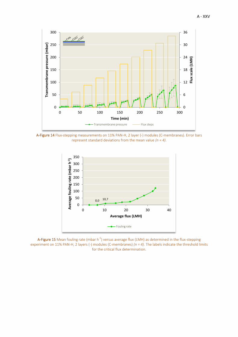
A - XXV

A-Figure 14 Flux-stepping measurements on 11% PAN-H, 2 layer (-) modules (C-membranes). Error bars

represent standard deviations from the mean value (n = 4).


) versus average flux (LMH) as determined in the flux-stepping experiment on 11% PAN-H, 2 layers (-) modules (C-membranes) (n = 4). The labels indicate the threshold limits

for the critical flux determination.

0

6

12

18

24

30

36

0

50

100

150

200

250

300

0 50 100 150 200 250 300

Flu

x sc

ale

(LM

H)

Tran

sme

mb

ran

e p

ress

ure

(m

bar

)

Time (min)


0,0 10,7

0

50

100

150

200

250

300

350

0 10 20 30 40 Ave

rage

fo

ulin

g ra

te (

mb

ar h

-1)

Average flux (LMH)

Fouling rate

A - XXVI




A-Figure 16 Evolution of the transmembrane pressure (mbar) of the module replicates of 11% PAN-H (-) during

Fouling Period 1. Arrows indicate time points of biofilm sampling.

A-Figure 17 Evolution of the transmembrane pressure (mbar) of the module replicates of 11% PAN-H, 1 layer (+)

during Fouling Period 1. Arrows indicate time points of biofilm sampling.

0

100

200

300

400

500

600

700


Tran

sme

mb

ran

e p

ress

ure

(m

bar

)

Date



0

100

200

300

400

500

600

700


Tran

sme

mb

ran

e p

ress

ure

(m

bar

)

Date



A - XXVII

A-Figure 18 Evolution of the transmembrane pressure (mbar) of the module replicates of 11% PAN-H, 2 layers (-)

during Fouling Period 1. Arrows indicate time points of biofilm sampling.


3.2.1. DGGE fingerprinting of PCR-amplified 16S rRNA gene fragments

As seen from A-Tabel 2, the genomic DNA concentration of the sludge and of the biomass developing

at the membrane surfaces stayed approximately constant over time, except for 25-Nov14, which

corresponds to the first day the pristine membranes were immersed in the HT-MBR (first contact

moment between the membranes and the sludge biomass). The fluctuations in concentrations can be

attributed to different amount of samples scraped off from the membrane surfaces meant for DNA

extraction, or to some loss of material during processing of the samples. Since the concentration of

PCR amplicons was not constant, different volumes were loaded on the DGGE gel in order to analyse

approximately 300 ng per sample.

A-Tabel 2 Genomic DNA quantity (ng µl

-1) of the PCR amplicons of the sludge and the biofouling layer of the

different membrane types sampled at different time points and determined based on Qubit measurements. Values are given as (mean standard deviation) (n = 2 membrane replicates).

Genomic DNA concentration (ng µl-1

) at the sampling date

Sample 25-Nov14

(Day 72)

01-Dec14

(Day 78)

08-Dec14

(Day 85)

15-Dec14

(Day 92)

19-Dec14

(Day 96)

02-Jan15

(Day 110)

13% PAN

(neutral) / 20.0 0.6 13.7 5.0 24.8 0.6 20.1 2.4 35.3 8.1

11% PAN-H,

(-) / 28.2 2.6 24.2 2.3 25.1 4.1 16.7 2.6 28.7 4.1

11% PAN-H,

1 layer (+) 5.1 1.6 13.9 1.1 4.5 0.2 6.3 0.1 46.2 2.3 72.6 2.0

11% PAN-H,

2 layers (-) 4.2 0.2 27.2 1.4 46.9 5.8 61.4 8.8 62.3 4.4 59.5 1.3

Sludge 49.1 3.5 51.8 9.3 32.0 0.3 31.5 3.6 32.1 2.4 49.5 5.2

0

100

200

300

400

500

600

700


Tran

sme

mb

ran

e p

ress

ure

(m

bar

)

Date



A - XXVIII

As seen from A-Tabel 3, the concentration of genomic DNA of the protamylasse feed samples

increased with time from day 1 (feed freshly prepared in disinfected vessel) during the maintenance

period, and eventually reached a final concentration of around 100 ng µl-1 on day 8, indicating

bacterial development in the feed vessel. This observation was supported by the microscopic

investigation of the feed solution (Chapter 4, Section 1.3) and attributed to the non-sterile working

conditions enhancing bacterial growth in nutrient rich environments (Chapter 4, Section 3.1.1).

A-Tabel 3 Genomic DNA quantity (ng µl-1

) of the PCR amplicons of the protamylasse feed solution sampled at different time points during two maintenance periods and determined based on Qubit measurements. Values are given as (mean standard deviation) (n = 2). No replicate measurement was performed on the feed pellet

developing at the bottom of the feed vessel.

Day of the maintenance period Genomic DNA concentration (ng µl-1

)

Day 1 /

Day 2 10.4 1.5

10.8 0.8

Day 3 46.7 2.7

61.9 4.1

Day 4 101.5 4.9

Day 8 98.1 2.7

Feed pellet 95.6

A-Figure 19 AGE gel of the PCR products obtained by electrophoresis on a 1.5% agarose gel and stained with GelRed, run against a GeneRuler 100 bp plus DNA-ladder.

A - XXIX

A-Figure 19 represents the AGE gel obtained by electrophoresis of the PCR amplicons of the sludge,

membrane and protamylasse feed samples. The NC (lane n° 21 of row D) showed no signal, indicating

absence of contamination during sample handling and processing. The majority of the bands hold a

substantial amount of DNA and are not preceded by a smear of degraded RNA. Since the extracted

DNA of all samples was amplified with the same forward and reverse primers, the position of the PCR

amplicons is approximately on a horizontal line corresponding to the migration distance of the 400 to

500 bp sequence of the reference ladder (lane n° 1 and 22 of rows A, B, C and D), as expected. Small

fluctuations from the horizontal line are due to differences in genomic DNA concentration, which

makes high concentration bands appear more prominent and at a greater downward distance than

low concentration bands.

A-Tabel 4 Attribution of the lanes of the AGE gel presented in A-Figure 19 (membrane and sludge samples).

Sampling date

25-Nov14

(Day 72)

01-Dec14

(Day 78)

08-Dec14

(Day 85)

15-Dec14

(Day 92)

19-Dec14

(Day 96)

02-Jan15

(Day 110)

Row Sample Lane number

A

13% PAN

(neutral) 2, 4 3, 5

11% PAN-H (-) 6, 8 7, 9

11% PAN-H,

1 layer (+) 10, 12 11, 13

11% PAN-H,

2 layers (-) 14, 16 15, 17

Sludge 18, 20 19, 21

B

13% PAN

(neutral)

2, 4

3, 5

11% PAN-H (-) 6, 8 7, 9

11% PAN-H,

1 layer (+) 10, 12 11, 13

11% PAN-H,

2 layers (-) 14, 16 15, 17

Sludge 18, 20 19, 21

C

13% PAN

(neutral)

2, 4

3, 5

11% PAN-H (-) 6, 8 7, 9

11% PAN-H,

1 layer (+) 10, 12 11, 13

11% PAN-H,

2 layers (-) 14, 16 15, 17

Sludge 18, 20 19, 21

A - XXX

A-Tabel 5 Attribution of the lanes of the AGE gel presented in A-Figure 19 (protamylasse feed samples).

Row Day of the maintenance period Lane number3

D

Day 1 2, 3

Day 2 4, 5, 16, 17

Day 3 6, 7, 18, 19

Day 4 10, 11

Day 8 14, 15

Feed pellet 20

҉ Summarized, Qubit measurement and AGE visualisation of the PCR products obtained from

genomic DNA extracted from the activated sludge, protamylasse feed and membrane biofilm samples

did indicate relatively stable DNA concentrations throughout the experimental period and DNA

sequences of between 400 and 500 bp, and thus allowed for further use in DGGE fingerprinting

analysis. The negative control showed no signal.

3 Lane numbers 8, 9, 12 and 13 are of no meaning for this work.

A - XXXI

Appendix 2: Risk assessments

PAN membrane preparation/characterization

Membrane potting

Continuous filtration experiment

COD measurement

TN measurement

Phosphate measurement

Biofouling characterization by SEM

The risk assessments were submitted to [email protected].

A - XXXII

A - XXXIII

Appendix 3: List of products

Reagens Bruto formula CAS n° Supplier references

Membrane and module preparation

Binder, contains epoxy resin / / UHU plus, endfest 300 90.5 gr/75 ml

Dimethyl sulfoxide, zur Analyse C2H6OS 67-68-5 Acros Organics

Hardener, contains N,N-dimethyldipropylenetriamine

/ 10563-29-8 UHU plus, endfest 300 72.5 gr/75 ml

Poly(acrylic acid, sodium salt) solution, 35 wt% in H2O

(C3H4O2)x.(C3H3O2)y.yNa 9003-04-7 Sigma-Aldrich 416037-100ML Average Mw = 15.000 g/mol

Poly(allylamine hydrochloride) (C3H2N)n.HCl 71550-12-4 Sigma-Aldrich 283215-5G Average Mw = 15.000 g/mol

Polyacrylonitrile (C3H3N)n 25014-41-9 Scientific Polymer Products Inc. Average Mw = 150.000 g/mol

Sodium hydroxide - pearl, analytical reagent grade

NaOH 1310-73-2 Fisher Chemical 1KG

Sodium nitrate a.r. NaNO3 7631-99-4 Chem-Lab NV 1KG

Operating conditions of the lab-scale MBR system

2-propanol C3H8O 67-63-0 Hach Lange GMBH LCK 138

4-chloor-3,5-dimethylfenol = chloroxylenol

C8H9ClO 88-04-0 DettolMedical chloroxylenol 4.9%, antiseptum-desinfectans 1L

Dipotassium peroxodisulfate K2S2O8 7727-21-1 Hach Lange GMBH LCK 138

Disodium tetraborate Na2B4O7 1330-43-4 Hach Lange GMBH LCK 138

Mercury(ll)sulfate HgSO4 7783-35-9 Hach Lange GMBH LCK 314

Phosphoric acid, 33% H3PO4 7664-38-2 Hach Lange GMBH LCK 138

Sodium hydroxide NaOH 1310-73-2 Hach Lange GMBH LCK 138

Sodium hypochlorite NaClO 7681-52-9 Aqueous solution containing 3.6% active chlorine, 15° Chl (Javel) Delhaize, 2L

Sodium hypochlorite solution, reagent grade

NaClO 7681-52-9 Sigma-Aldrich 425044-1L Available chlorine 10-15%

Sodium metaborate NaBO3.4H2O 10486-00-7 Hach Lange GMBH LCK 349

Sodium peroxodisulfate Na2S2O8 7775-27-1 Hach Lange GMBH LCK 349

Sodiumazide NaN3 26628-22-8 Hach Lange GMBH LCK 138

Sulfuric acid, 11% H2SO4 7664-93-9 Hach Lange GMBH LCK 349




A - XXXIV


Membrane performance measurement Methylene blue C16H18N3S.Cl 61-73-4 /

Biofouling (community) characterization 0.5M EDTA C10H12FeN2NaO8 60-00-4 /

1M Tris.Cl, pH 8.0 (Trizma base: C4H11NO3) (Trizma base: 77-86-1) (Trizma-base: Sigma-Aldrich, T6066-1KG)

25:24:1 phenol-chloroform-isoamyl alcohol mixture; BioUltra, for molecular biology

/ 136112-00-0 Sigma-Aldrich 77617-500ML

2-propanol molecular biology grade

C3H8O 67-63-0 AppliChem

50x TAE Tris/Acetic Acid/EDTA Buffer

/ Tris acetate: 6850-28-8; EDTA: 60-00-4

Bio-Rad Laboratories 1l

6x LD, 6x DNA Loading Dye / / Thermo Scientific 1 ml

AccuStart ll PCR ToughMix / / Quanta Sciences inc. 1.25 ml

Acrylamide/N,N'-Methylenebisacrylamide 37.5:1; for biochemistry; 40% mix solution in water

(C7H10N2O2.C3H5NO)n 25034-58-6 Acros Organics 500 ml

Ammonium persulphate / 7727-54-0 Bio-Rad Laboratories 10g

Cetrimide (=hexadecyltrimethyl ammonium bromide)

C19H42BrN 57-09-0 Sigma-Aldrich H9151-25G

Di-sodiumhydrogen phosphate PA

Na2HPO4 7558-79-4 /

DNAse and RNAse free water / / The Epigenetics Company Zymo Research 10 ml

Ethanol absolute C2H6O 64-17-5 AnalaR NORMAPUR VWR BDH Prolabo

Formamide, 99.5%; for analysis CH3NO 75-12-7 Acros Organics 100 ml

Forward primer (GC-63F) / / J.T'SYEN

GeneRuler 100 bp plus DNA Ladder, 0.5 µg/µl

/ / Thermo Scientific 50 µg

Glutaraldehyde solution, Grade ll, 25wt% in H2O

C5H8O2 111-30-8 Sigma-Aldrich G6257-1L

Lysozyme chloride form, from chicken egg white

47400 units/mg solid 54500 units/mg protein (UV)

9066-59-5 Sigma-Aldrich L2879-5G

Magnesium sulphate heptahydrate

MgSO4.7H2O 10034-99-8 Merck 1kg

Proteinase K / 39450-01-6 AppliChem Pancrea MM = 27000 g/mol

Qubit dsDNA BR Buffer / / Life Technologies Invitrogen 50 ml

A - XXXV


Biofouling (community) characterization (continued)

Qubit dsDNA BR Reagent, 200x concentrate in DMSO

/ / Life Technologies Invitrogen 250 µl

RedGel Nucleic Acid Stain, 10000x in DMSO

/ / Biotium 0.5 ml

Reverse primer (518R) / / J.T'SYEN

RNAase A, 100 mg/ml / / Qiagen 1.25 ml

Sdium dihydrogenphosphate.1H2O PA 99%

NaH2PO4.H2O 10049-21-5 Merck 500g

Sodium chloride NaCl 7647-14-5 AnalaR NORMAPUR VWR BDH Problabo

Sodium dodecyl sulfate C12H25NaO4S 151-21-3 Sigma-Aldrich 71729-500G

SYTO® 62 Red Fluorescent Nucleic Acid Stain - 5 mM Solution in DMSO

/ / Life Technologies Invitrogen

SYTO® 9 Green Fluorescent Nucleic Acid Stain

/ / Life Technologies Invitrogen

TEMED, N,N,N',N'-tetramethylethylene-diamine

C6H16N2 110-18-9 Bio-Rad Laboratories 5 ml

Ultra Pure Agarose / 9012-36-6 Invitrogen

Urea; powder, BioReagent, for molecular biology, suitable for cell culture

CH4N2O 57-13-6 Sigma-Aldrich U5378-1KG

α-D-glucose, 96% anhydrous C6H12O6 492-62-6 Sigma-Aldrich 158968-500G

A - XXXVI

A - XXXVII

Appendix 4: CTAB protocol

Adapted CTAB-lysozyme method for genomic DNA extraction

Based on [32]

A. Transfer the sample suspension in 450 μl GTE buffer to a sterile 2-ml microcentrifuge tube

containing 50 μl of a 10 mg ml-1 lysozyme solution.

EDTA binds heavy metals and forms complexes with bivalent cations, thus destabilizing the cell membrane. It

inhibits deoxyribonuclease thus prevents DNA to be broken up. Glucose increases the osmotic pressure and

enhances cell lysis. The lysozyme solution was prepared in MQ instead of 25 mM Tris.Cl. Lysozyme weakens the

peptidoglycan cell wall and permits water to enter the cell, thus causing lysis.

B. Mix gently and incubate 1 h at 37 °C at 900 rpm shaking speed (MB-102, ThermocCell Mixing Block,

Bioer).

C. Make a 2:1 solution (v/v) of 10% SDS solution and 10 mg ml-1 proteinase K in MQ. Add 150 μl of this

solution to the cells and mix gently. Incubate 40 min at 55 °C at 900 rpm shaking speed.

SDS is an anionic detergent destroying de cytoplasmatic membrane of the cells. Proteinase K destroys proteins.

Plasmids and chromosomal DNA are released from the cells.

D. Add 1 µl RNAase A.

Destruction of the RNA released from the cell.

E. Add 200 μl of 5 M NaCl and mix gently.

NaCl blocks the binding of DNA to cetrimide.

F. Preheat CTAB solution to 65 °C in a water bath (RTE-101, Neslab), add 160 μl, and mix gently.

Incubate 10 min at 65 °C in a water bath.

G. Add an equal volume (∼1 ml) 25:24:1 (v/v) phenol/chloroform/isoamyl alcohol, shake vigorously to

mix, and microcentrifuge for 5 min at 12 000 rcf and 4 °C (Centrifuge 5424, Eppendorf or Mikro

200R, Hettich Zentrifugen).

The aqueous (upper) layer (isoamyl alcohol) contains the DNA. The apolar (bottom) layer (phenol/chloroform)

contains the undesirable organic compounds (lipids, proteins, polysaccharides, etc.).

H. Transfer 900 μl aqueous layer to a fresh sterile 2-ml microcentrifuge tube.

I. Repeat extraction with 25:24:1 (v/v) phenol/chloroform/isoamyl alcohol, shake vigorously to mix,

and spin in microcentrifuge for 5 min at 12 000 rcf and 4 °C..

J. Transfer 800 μl to fresh sterile 1.5-ml microcentrifuge tube.

CAUTION: For BSL3 organisms, dip tube in a disinfectant such as Vesphene IIse to disinfect outer surface. From this

point on, the supernatant can be processed in a BSL-2 laboratory (see Strategic Planning).

K. To 800 μl aqueous layer, add 560 μl (0.7 vol) isopropanol, mix gently by inversion until the DNA has

precipitated out of solution.

Precipitation of DNA.

A - XXXVIII

L. Incubate 30 min at room temperature. Microcentrifuge for 15 min at 12 000 rcf, room

temperature.

M. Aspirate supernatant and add 1 ml of 70% ethanol in MQ to wash DNA pellet. Mix gently by

inversion and microcentrifuge 5 min at 12 000 rcf at room temperature.

DNA is washed in order to remove precipitated salts.

N. Carefully aspirate supernatant, avoiding the pellet, and air-dry DNA pellet for 2 min. Do not

overdry.

O. Add 30, 50 or 100 μl TE buffer (10 mM Tris.HCl, 0.1 mM EDTA in MQ, pH 8.23), depending on size

of DNA pellet, to dried DNA pellet and store overnight at 4 °C to allow pellet to dissolve. Store up to

1 year at −20 °C.

RNase A can be added to TE (1 μg/ml) to reduce RNA contamination.

A - XXXIX

Appendix 5: Polarized summary

Traditional wastewater treatment installations, abbreviated as CASP, have the disadvantages of for

instance not being capable of delivering high quality water at all times as well as requiring a lot of

space. Therefore alternative technologies have been developed, including membrane bioreactors,

abbreviated as MBRs, using membranes through which the wastewater is filtered in combination with

so-called activated sludge containing microorganisms that perform the biodegradation of the

pollutants. However this technology is not perfect either. It has high investment costs, but most

importantly, the pores of the membranes can be filled up or covered by particles as well as

microorganisms, thus blocking the water from passing through. This phenomenon is more commonly

referred to as ‘fouling’ or biofilm formation. Fouling leads to high energy demands and related costs in

order to prevent, to diminish or to remediate the phenomenon. Moreover it prevents the broader

market development of the MBRs. A lot of researchers already have tried to find efficient anti-fouling

strategies. However the underlying processes are still unclear as well as the knowledge of the relation

between the microorganisms and the membranes, referred to as biofouling.

The main goal of this study was to gather knowledge about the relation between the microorganisms

and the membrane surface. The used membranes were made of polyacrylonitrile (PAN), a synthetic

molecule, and some of them were chemically modified as to bear either a positive or negative charge.

The membranes were placed during 40 days inside a laboratory-scale MBR, which was fed with

protamylasse, a by-product of the potato industry. The physico-chemical properties of the membranes

themselves were determined by means of several techniques (ATR-FTIR, SEM, AFM, CAM, volume

porosity measurement, electrokinetic measurement), but also their performance was analyzed in

terms of permeability (via CWP) and fouling tendency (via critical flux measurements). The

microorganisms in the MBR which interacted with the membranes and developed upon their surfaces

were characterized on a molecular level (referred to as PCR-DGGE fingerprinting) but also their

chemical properties and morphology were determined (via ATR-FTIR, SEM, CLSM).

The results revealed that the membranes differed from each other only in terms of surface charge and

membrane material (as a result of the chemical modifications applied), but that they were similar in

terms of physical properties (including pore size, permeability and surface roughness). The molecular

investigations indicated that the microorganisms growing in the biofilm at the membrane surface

were different from the ones present in the activated sludge of the MBR. Next it seemed that the

community of microorganisms in the biofilm evolved with time, but that all membranes housed the

same community at a certain moment in time. These observations allow concluding that certain

microorganisms are more prone to colonize membrane surfaces than others and that the surface

charges of the membranes do not play a decisive role in the selection of these microorganisms. These

observations might help the scientific community to develop more efficient anti-fouling strategies.

Keywords: membrane bioreactor, polyacrylonitrile, surface charge, biofouling, PCR-DGGE fingerprinting.

biofouling in membrane bioreactors: nexus between ... · nexus between polyacrylonitrile surface...

Documents