biodiversity of intertidal soft-sediment habitats in the ......biodiversity of intertidal...

Biodiversity of intertidal soft-sediment habitats in the Auckland Region

NIWA Client Report: HAM2009-097 June 2009 NIWA Project: DOC09302

All rights reserved. This publication may not be reproduced or copied in any form without the permission of the client. Such permission is to be given only in accordance with the terms of the client's contract with NIWA. This copyright extends to all forms of copying and any storage of material in any kind of information retrieval system.

Biodiversity of intertidal soft-sediment habitats in the Auckland Region Judi Hewitt Scott Edhouse Julia Simpson

NWA contact/Corresponding author

Judi Hewitt

Prepared for

Department of Conservation NIWA Client Report: HAM2009-097 June 2009 NIWA Project: DOC09302

National Institute of Water & Atmospheric Research Ltd Gate 10, Silverdale Road, Hamilton P O Box 11115, Hamilton, New Zealand Phone +64-7-856 7026, Fax +64-7-856 0151 www.niwa.co.nz

Contents Executive Summary iv 1. Introduction 1 2. Methods 5

2.1 Sample areas 5 2.2 Sampling 5 2.3 Habitat types 6 2.4 Diversity definitions 7 2.5 Diversity calculations 8

3. Average habitat diversity at the replicate scale 10 3.1 Southern Kaipara 10 3.2 Kawau Bay 10 3.3 Mahurangi Harbour 13 3.4 Weiti Estuary 13 3.5 Okura Estuary 13 3.6 Central Waitemata Harbour 17 3.7 Upper Waitemata Harbour 17 3.8 Whitford Embayment 20 3.9 Tamaki Strait 20

4. Species accumulation rates and total species richness of habitats 23 4.1 Southern Kaipara 23 4.2 Kawau Bay 24 4.3 Mahurangi Harbour 25 4.4 Karepiro Bay (Weiti and Okura Estuaries) 26 4.5 Waitemata Harbour (Central and Upper) 27 4.6 Whitford Embayment 28 4.7 Tamaki Strait 29

5. Effect of scale on diversity 31 5.1 Within-habitat heterogeneity 31 5.2 Habitat, site and replicate comparisons 35

6. Summary of results 40 6.1 Patterns apparent at the replicate core scale 40 6.2 Diversity at the habitat scale 40 6.3 Bullet point summary 41 6.4 Conclusions 42

7. Acknowledgements 43 8. References 44

Reviewed by: Approved for release by:

Carolyn Lundquist Neale Hudson

Formatting checked

Biodiversity of intertidal soft-sediment habitats in the Auckland Region iv

Executive Summary

The allocation of Marine Protected areas is a major conservation and management priority in New

Zealand. This task requires some determination of both representativeness and uniqueness of areas in

terms of their biodiversity and ecology. At present, while the role of habitats at a smaller-scale is

considered, the main focus of the classifications is on habitats described by environmental variables

(depth and substrate type) rather than including biotic factors. In part, this emphasis is driven by a

lack of information both about the effect of biogenic habitats on diversity and on the distribution of

such habitats. This project seeks to remedy the lack of information regarding key-habitat forming

species on biodiversity in the soft-sediment intertidal zone, a particular information gap identified by

the Biodiversity and Biosecurity Outcome Based Investment (OBI). The habitats used in the study

included both environmentally driven (i.e., those defined by the Ministry of Fisheries (MFish) and

Department of Conservation (DoC)) and biogenic habitats. Data was available for six habitats:

Cockles, Macomona, Mud, Sand (medium to fine particle size), Seagrass and Tubeworms.

We found no strong patterns in alpha diversity (i.e., the average number of species per core) between

the habitats that applied across all locations. However, Cockle habitats were more likely to have a high

alpha diversity, closely followed by Seagrass and Tubeworm habitats. Importantly, the habitats

described by sediment characteristics (as mud and sand) were most likely to have a low alpha

diversity.

Gamma diversity (i.e., the total number of species predicted for a habitat if 100 samples were

collected) also showed no consistent patterns between the habitats across locations. The Tubeworm

and Cockle habitats were most likely to have high gamma diversity, while the Mud habitat most

frequently had the lowest gamma diversity.

The differences we observe between the replicate and habitat scale, in which habitats have more

species richness, are driven by the within-habitat heterogeneity. This is controlled by the number of

infrequently occurring species (beta diversity). Two consistent patterns were observed: the Seagrass

habitat never exhibited the highest or lowest beta diversity; and within sites, the species found in

individual cores varied little for the Cockle habitat at all locations.

While we did not find consistent patterns of diversity among different habitats, our results suggest that

some species do provide a habitat for other species and can, therefore, affect biodiversity. In

particular, the New Zealand cockle, seagrass and the mats created by maldanid and polydorid

tubeworms. Location-specific variables, rather than regional species pools, seemed to be most

important for controlling the effect of the relationship between a habitat and its biodiversity. This

highlights the need to preserve a variety of habitats rather than concentrating on those habitats that are

considered to be of high biodiversity. Indeed preserving habitat diversity at a variety of scales is likely

to be the key to conserving biodiversity and ecosystem function.

Biodiversity of intertidal soft-sediment habitats in the Auckland Region 1

1. Introduction

Recently, the Ministry of Fisheries (MFish) and the Department of Conservation

(DoC) defined important habitat types for biodiversity conservation and mapping

(Ministry of Fisheries and Department of Conservation 2008). These were based on a

few sedimentary types and depth categories, e.g., mud, sand, intertidal, <20 m depth

etc. However, such broad-scale habitat definitions blur over the small-scale

preferences exhibited by many benthic macrofaunal species. Particularly in soft-

sediments, biogenic habitats can be important for biodiversity, with many rare species

exhibiting habitat specificity (Ellingsen et al. 2007, Hewitt et al. 2005, Thrush et al.

2006a).

There is surprisingly little New Zealand data available from which to determine which

habitat features of intertidal coastal areas are of particular importance to biodiversity.

Although there are many popular accounts that assert the importance of specific

biogenic habitats, few of these accounts have quantified diversity. Early work in New

Zealand focussed on description of assemblages (see Rowden et al. 2007 for a review)

rather than biodiversity estimates per se. Assessments of effects of marine reserves

generally focus on species-specific comparisons of abundance and size. Assessments

of biodiversity have been made in some marine areas of New Zealand, e.g.,

MacDiarmid (2006) and Rowden et al. (2007); however, these assessments are

focussed on specific groups of organisms and/or determining the location of

biodiversity hotspots, rather than habitat dependency.

This project supports the research on biodiversity, habitat diversity and species

richness in estuaries and coasts within the Biodiversity & Biosecurity OBI. Work

within the OBI determined that while knowledge of biodiversity of many New

Zealand marine habitats was generally lacking, knowledge of biodiversity in the

habitats occurring within intertidal soft-sediment areas was particularly sparse. The

habitats to be utilised were chosen to include both environmentally determined (i.e.,

those defined by MFish and DoC) and biogenic habitats that had been proven to have

effects on macrofaunal species, or that were considered to be important species for

other reasons: mangroves, seagrass meadows, cockle beds (Austrovenus stutchburyi),

tubeworm mats (Cummings et al. 1993, Thrush et al. 1996), Macomona liliana beds

(Pridmore et al. 1990, Thrush et al. 2006b), pipi beds (Paphies australis) and shrimp

burrows (Berkenbusch et al. 2007). Available data reduced this list of habitats to six:

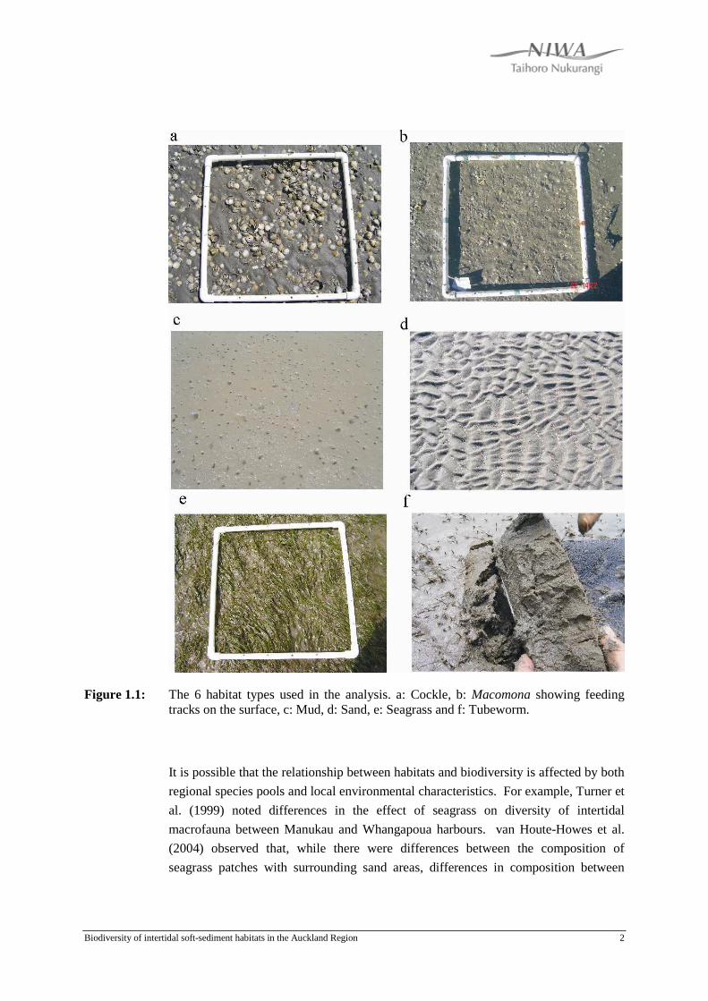
cockles, Macomona, mud, sand (medium to fine particle size), seagrass and

tubeworms (Fig. 1.1).


Figure 1.1: The 6 habitat types used in the analysis. a: Cockle, b: Macomona showing feeding tracks on the surface, c: Mud, d: Sand, e: Seagrass and f: Tubeworm.

It is possible that the relationship between habitats and biodiversity is affected by both

regional species pools and local environmental characteristics. For example, Turner et

al. (1999) noted differences in the effect of seagrass on diversity of intertidal

macrofauna between Manukau and Whangapoua harbours. van Houte-Howes et al.

(2004) observed that, while there were differences between the composition of

seagrass patches with surrounding sand areas, differences in composition between


harbours was greater still. Lundquist et al. (2003) noted that while diversity of muddy

estuarine intertidal areas was generally expected to be lower than that of sandy areas,

location-specific sedimentation rates were an important factor. Sites with higher

sedimentation rates exhibited lower diversity, independent of grain size. For this

reason, only locations where most of the habitats present had been sampled were

considered in this project (Fig. 1.2). Furthermore, habitat types had to be defined at the

scale of the site prior to sampling of sediment. A search was made for coastal

locations for which the majority of their intertidal areas had been sampled in the past

10 years. Data from these locations were investigated to determine whether most of

the habitats were present and whether samples had been collected in a consistent

fashion. Because the aim of the study was the calculation of biodiversity, it was

imperative that data of high taxonomic resolution were used. This resulted in the

exclusion of some locations. In a few cases, locations had been sampled but not yet

analysed, and in another case the results had already been published (Alfaro 2006).

Figure 1.2: Coastal locations for which information was available.


This report investigates the relationship between different types of diversity (species

richness, evenness and diversity indices) relative to key habitat types and habitat

forming species (mud, sand, seagrass, cockle beds, wedge shell beds and tube-worm

beds). Results are presented for nine North Island locations around the Auckland area:

Southern Kaipara, Kawau Bay, Mahurangi Harbour, Weiti Estuary, Okura Estuary,

Upper Waitemata Harbour, Central Waitemata Harbour, Whitford Embayment and

Tamaki Strait (Fig. 1.2). Insight gained from this analysis will be useful in:

• defining appropriate measures of biodiversity;

• illustrating the efficacy of rapid assessment techniques for determining

habitats; and

• demonstrating the value of maintaining habitat diversity.


2. Methods

2.1 Sample areas

Intertidal soft-sediment benthic macrofauna information was available for 9 North

Island locations (Southern Kaipara, Tamaki Strait, Whitford Embayment, Okura

Estuary, Kawau Bay, Weiti Estuary, Mahurangi Harbour, and the Central and Upper

Waitemata Harbour (see Fig. 1.2)). All of these coastal areas are within 100 km of

each other. The Southern Kaipara is in a different regional species pool, being on the

west coast, while all the other locations are on the east coast of the North Island.

Sampling of each location had been carried out under different studies, often in

different years (Table 2.1), but all samples were collected using a 13 cm diam., 15 cm

deep corer.

Table 2.1: Information on the data available. ARC contact Grant Barnes, NIWA contact Judi Hewitt Marine Ecology group, Hamilton.

Location Area to mean high water (km2) Estuary Type Year(s) sampled Data holder

Southern Kaipara Harbour

440 Drowned Valley 2004 ARC

Kawau Bay 121.5 Coastal Embayment

2006 ARC

Mahurangi Harbour 24.57 Drowned Valley 1994 - ongoing

2005-6

ARC

NIWA

Okura Estuary 1.36 Tidal Lagoon 1999 NIWA

Weiti Estuary 2.83 Tidal Lagoon 2008 ARC

Upper Waitemata Harbour

Drowned Valley 2003-ongoing ARC

Central Waitemata Harbour

Drowned Valley 2000-ongoing

2006

ARC

NIWA

Whitford Embayment

11.06 Drowned Valley 2000

2000-1

ARC

NIWA

Tamaki Strait 335.36 Coastal Embayment

2002, 2007-8

2001, 2006

ARC

NIWA

2.2 Sampling

The number of replicates collected at a site varied from 3 to 12. Where more than 3

replicates were collected, 3 replicates were randomly chosen. In all studies, the

benthic macrofauna had been identified in the same laboratory to the same taxonomic


level (generally species) and enumerated. More importantly, different studies used

differing mesh sizes (either 1 mm or 0.5 mm). Fortunately, in the four locations for

which the 1 mm mesh was not the primary method there had been some studies using

both mesh sizes. This information was used to determine the species found when a

0.5 mm mesh was used that were not found when a 1 mm mesh was used, and these

species were removed from the data before analysis.

2.3 Habitat types

For all the studies used, the core data was accompanied by general habitat

descriptions, mainly consisting of biogenic features.

Six habitat types were common enough for analysis: seagrass meadows and patches

(Zostera muelleri), tube worm beds (most frequently the spionid polychaete Boccardia

syrtis, but also the maldanid polychaetes Macroclymenella stewartensis and Asychis

spp.), adult cockle beds (Austrovenus stutchburyi >20 mm longest shell dimension),

adult wedge shell beds (Macomona liliana >20 mm longest shell dimension),

unvegetated mudflats (>20% mud content) and unvegetated fine-sand (>80% fine-

medium sand) flats that did not contain sufficient densities of cockles, Macomona or

tubeworms to be allotted to one of these habitats. This definition of the Sand habitat

may result in low species richness simply because of the exclusion of cockles,

Macomona and tubeworms (common intertidal species) from their species lists.

Habitats based on fauna were defined as follows: Tubeworm >5 in a 20 x 20 cm

quadrat; Austrovenus > 5 in a quadrat; Macomona >5 feeding tracks in 2 quadrats. In a

few cases a site belonged to more than one faunal habitat type (e.g., cockles and

Macomona or tube worms-Macomona) and the site was allocated to both habitat

types. Seagrass habitats frequently contained cockles and Macomona but were

defined as Seagrass only, in order to aid comparisons with other published studies.

All of the habitats occurred at 4 of the locations. No seagrass occurred at Okura

Estuary, Weiti Estuary, Upper Waitemata Harbour and Whitford Embayment and

while a patch occurred in the Central Waitemata, it had not been sampled. The

Tubeworm habitat did not occur in Okura and the Macomona habitat was not found in

the Upper Waitemata Harbour. Generally, 3 – 9 sites had been sampled from each

habitat in each location but only one site was found for the Macomona habitat in the

Central Waitemata Harbour, the Sand habitat in Mahurangi Harbour and the

Tubeworm habitat in Weiti Estuary.


A number of other habitats were recorded but either occurred infrequently in an area

or did not occur in many of the areas. It is also possible that a number of biogenic

habitats were not recognised as such when sampling.

2.4 Diversity definitions

Many methods exist for measuring biodiversity. Of these, the most used is species

richness or, more simply, the number of species. Even this simple measure can be

expressed in a number of ways: average number of species observed; total number of

species observed, Margalef’s species richness, and number of species predicted, using

species accumulation curves, from a set number of samples (Colwell & Coddington

1994), areas (Ugland et al. 2003) or habitats (Thrush et al. 2006a).

In both terrestrial and marine systems, most individuals belong to a few abundant

species and most species are represented by a small number of individuals. Thus

another way to consider biodiversity is how abundances are distributed amongst

species (Pielou’s evenness). Low evenness generally indicates dominance by a single

species.

A number of indices have been developed to combine both the number of species and

evenness. Of these, the most frequently used is the Shannon-Weiner index.

Shannon-Weiner is a logarithmic index and care must be taken when making

comparisons between studies to ensure that a similar log base has been used (here we

use loge). The second most frequently used is Simpson’s index, calculated simply

from probabilities of occurrence. The Shannon-Weiner index is more sensitive to rare

species, while Simpson’s index is more sensitive to more abundant species.

Measures can also be made at a number of different scales: alpha or gamma. The

frequency distributions of species observed are typically strongly right-skewed, with a

large number of species present in only a few samples. Thus much of biodiversity as

measured by species number is represented by rare (infrequently occurring species).

How these species are spatially distributed and what proportions they represent

primarily affect the difference between the average and total number of species. The

average number of species is often termed alpha diversity, the total number of

species, gamma diversity and the difference between the two, beta diversity (Crist et

al. 2003, Klimek et al. 2008, Lande 1996). The latter is a representation of how

heterogeneous the sampled area is. Note that species turnover along a gradient can

also be termed beta diversity; in this case it is generally calculated as the ratio of the

average to the total number of species (Ricotta 2008, Whittaker 1960).


2.5 Diversity calculations

A number of diversity measures were calculated at the replicate level: species

richness, evenness, Shannon-Weiner and Simpson index (Primer E, Clarke & Gorley

2006), from which the average at each site was reported. The statistical significance of

differences between habitats in each location was determined by one-way ANOVA

with habitat as a fixed factor. Averages and standard errors were calculated for each

habitat in each location.

Species richness and evenness were calculated at three spatial scales:

• The replicate (within-site) scale. Number of species and evenness of the

distribution of individuals across species were calculated for each replicate.

• The site scale. Number of species and evenness of the distribution of

individuals across species were calculated for the sum of the three replicates at

each site. Averages of these were then calculated for each habitat in each

location.

• The habitat scale.

o Evenness of the distribution of individuals across species was

calculated for the sum of the sites in each habitat in each location.

o Species richness was determined by prediction as it is highly

dependent on numbers of samples and each habitat had a different

number of samples, due to the different number of sites available for

each habitat. We derived species accumulation curves for each

habitat in each location using the commonly used Mao Tau estimation

(EstimateS, Colwell 2006). As few of the species accumulation

curves reached an asymptote (i.e., in most cases collecting more

samples continued to increase the number of species observed), we set

total species richness (gamma diversity) as the number of species

predicted to be found if 100 samples had been collected. N = 100 was

chosen, as the degree of separation between the curves had largely

stabilised by this point. Furthermore, for these comparisons it was

necessary to have as many samples per habitat as possible. For this

reason, Okura and Weiti estuaries which both flow into Karepiro Bay

were combined, and the Upper and Central Waitemata were also

combined.


Beta diversity (heterogeneity of species richness occurring within each

habitat) was calculated as [total – average] species richness. Beta diversity

was calculated at two scales: within site; and within habitat.


3. Average habitat diversity at the replicate scale

3.1 Southern Kaipara

In the southern Kaipara, the average number of species found was significantly lower

in the Mud and Sand habitats than the others (Fig. 3.1). Seagrass and Tubeworms had

the highest average number of species, though these differences were not statistically

significant due to high variability in these habitats. No differences were detected in

the average number of individuals observed between the habitats, due to the high

variability between sites. All habitats exhibited high evenness (>0.74), with the Mud

habitat the least even and the Tubeworm habitat the most even. The Tubeworm

habitat also had the highest Shannon-Weiner and Simpson index, within the habitats in

the Southern Kaipara, followed by the Seagrass habitat, while the Sand habitat had the

lowest Shannon-Weiner index and the Mud habitat had the lowest Simpson index.

3.2 Kawau Bay

In Kawau Bay, the average number of species found in the Sand habitat was

significantly lower than the number found in the Seagrass and Tubeworm habitats

(Fig. 3.2). These two habitats had the highest average number of species (11.5 and 9.4

respectively). Some differences were detected in the average number of individuals

observed between the habitats, with the Sand and Macomona habitats having the

lowest numbers and the Cockle habitat the highest. All habitats, except the Cockle

habitat, exhibited high evenness (>0.79), with the Tubeworm habitat again being the

most even. The Seagrass habitat had the highest Shannon-Weiner index and the

Tubeworm habitat had the highest Simpson index, while the Sand habitat again had

the lowest Shannon-Weiner index and the Cockle habitat had the lowest Simpson

index.


Figure 3.1: Differences in diversity in Southern Kaipara Harbour based on six habitats.


Figure 3.2: Differences in diversity in Kawau Bay based on six habitats.


3.3 Mahurangi Harbour

In Mahurangi Harbour, the average number of species found was significantly lower

in the Seagrass and Tubeworm habitats than the Cockle habitat (Fig. 3.3). The Cockle

and the Sand habitats had the highest average number of species. No significant

differences were detected in the average number of individuals observed between the

habitats, due to the high variability between sites. All habitats exhibited high

evenness (>0.74), with the Mud habitat again the least even and the Seagrass habitat

the most even. The Cockle habitat had the highest Shannon-Weiner index and the

Seagrass had the highest Simpson index, while the Tubeworm habitat had the lowest

Shannon-Weiner and Simpson index.

3.4 Weiti Estuary

In Weiti Estuary, no Seagrass habitat was found. The average number of species found

was significantly higher in the Cockle habitat than in the all the other habitats (Fig.

3.4). No significant differences were detected in the average number of individuals

observed between the habitats, due to the high variability between sites. The Cockle

and the Macomona habitat exhibited a high evenness (> 0.74), while the remaining

habitats were less even. The Cockle habitat had the highest Shannon-Weiner

(statistically significant) and Simpson index, while the sand had the lowest Shannon-

Weiner and Simpson index.

3.5 Okura Estuary

In Okura Estuary, no Seagrass habitat was found and no Tubeworm habitats were

sampled. There were no significant differences between habitats in the average

number of species found due to high variability, however the Mud habitat exhibited

the lowest average number of species and the Cockle habitat exhibited the highest

average number of species (8.3 and 11.1 respectively), as shown in Fig. 3.5. Some

differences were also detected in the average number of individuals observed between

the habitats, with the Mud habitats having the lowest numbers and the Cockle habitat

the highest. All habitats exhibited high evenness > 0.74, with the Cockle habitat the

least even and the Mud habitat the most even. The Macomona habitat had the highest

Shannon-Weiner and Simpson index (although not significantly so).


Figure 3.3: Differences in diversity in Mahurangi Harbour based on six habitats.


Figure 3.4: Differences in diversity in Weiti Estuary based on five habitats.


Figure 3.5: Differences in diversity in Okura Estuary based on four habitats.


3.6 Central Waitemata Harbour

While a small area of seagrass does occur in the Central Waitemata Harbour area, this

had not been sampled. In the Central Waitemata Harbour, the average number of

species found in the Mud habitat was significantly lower than the others (Fig. 3.6).

The Cockle, Macomona and Tubeworm habitats had the highest average number of

species. Again no significant differences were detected in the average number of

individuals observed between the habitats, although the Mud and Sand habitats had

the lowest numbers and the Cockle habitat the highest. All habitats, except the Cockle

and Tubeworm habitat, exhibited high evenness, with the Sand habitat most even. The

Sand habitat also had the highest Shannon-Weiner and Simpson indices, followed by

the Macomona habitat, while the Mud habitat had the lowest Shannon-Weiner and

Simpson indices.

3.7 Upper Waitemata Harbour

In the Upper Waitemata Harbour, Seagrass and Macomona habitats are absent. The

Cockle habitat had the highest number of species and individuals (Fig. 3.7). However,

the Cockle habitat exhibited low evenness (<0.7); all others had evenness values

between 0.70 and 0.76. The Cockle habitat also exhibited a significantly higher

Shannon-Weiner diversity index than the Mud habitat, but there were no significant

differences in Simpson index between the four habitats.


Figure 3.6: Differences in diversity in Central Waitemata Harbour based on five habitats.


Figure 3.7: Differences in diversity in Upper Waitemata Harbour based on four habitats.


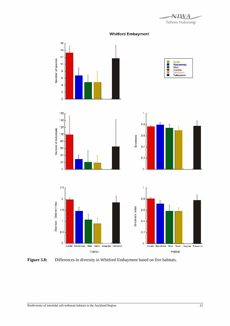
3.8 Whitford Embayment

Seagrass habitat is absent from the Whitford Embayment. The average number of

species found was significantly higher in the Cockle habitat than in the Macomona,

Mud and Sand habitats (Fig. 3.8). The average number of species found in the

Tubeworm habitat was not significantly higher than the other habitats due to high

variability. No differences were detected in the average number of individuals

observed between the habitats, due to the high variability observed in the Cockle and

Tubeworm habitats, although number of individuals was on average lower in the

Macomona, Sand and Mud habitats. Evenness ranged between 0.70 - 0.82, with the

Macomona habitat the most even. The Cockle habitat had the highest Shannon-Weiner

and Simpson index, followed by the Tubeworm habitat. The Sand and Mud habitats

had significantly lower Shannon-Weiner indices than the Cockle and Tubeworm

habitats, and also had the lowest Simpson index.

3.9 Tamaki Strait

In the Tamaki Strait, no significant differences were observed between habitats in the

average number of species found, with the average ranging between 6 and 10 (Fig.

3.9). No significant differences were detected in the average number of individuals

observed between the habitats, although the averages ranged between 18 and 50, due

to the high variability between sites. All habitats, except the Cockle habitat, exhibited

high evenness (> 0.74), with the Sand habitat being the most even. The Macomona

and the Mud habitats exhibited significantly higher Shannon-Weiner indices than the

Sand habitat and a significantly higher Simpson index than all the other habitats.


Figure 3.8: Differences in diversity in Whitford Embayment based on five habitats.


Figure 3.9: Differences in diversity in Tamaki Strait based on six habitats.


4. Species accumulation rates and total species richness of habitats

Species accumulation curves for each habitat in each location were derived as

described in the Methods using Mao Tau estimation. In Section 4, we describe the

behaviour of these species accumulation curves for the number of samples collected at

each site. These curves are used to estimate total species richness (gamma diversity)

for each habitat by extrapolating these species accumulation curves out to 100 samples

for each location.

4.1 Southern Kaipara

The species accumulation curves for the habitats in Southern Kaipara show that the

Seagrass habitat has the greatest number of species present (Fig. 4.1). This is followed

by the Tubeworm habitat, then Cockle and Macomona habitats. The Mud and

Macomona habitats initially increase at a greater rate than the Sand habitat but appear

to be reaching an asymptote earlier than the Sand habitat, which continues to increase

at a rate that will result in higher species richness than the Macomona and Mud

habitats.


Figure 4.1: Species accumulation curves for the different habitats in Southern Kaipara Harbour.

4.2 Kawau Bay

In Kawau Bay the Tubeworm habitat showed the greatest accumulation rate of species

(Fig. 4.2). The Cockle and Seagrass habitats have the next highest accumulation rates,

although the Seagrass habitat is reaching an asymptote while the Cockle habitat is

continuing to accumulate more species. The Mud habitat increased faster than the

Sand habitat at first but was flattening out, while the Sand habitat continued to

accumulate new species. The small number of samples taken in the Macomona

habitat makes it difficult to reach any conclusion, although it seems likely that the

species accumulation asymptote would lie between that of the Cockle and Sand

habitats (similar to the Southern Kaipara).


Figure 4.2: Species accumulation curves for the different habitats in Kawau Bay.

4.3 Mahurangi Harbour

In this location, the Cockle habitat exhibited the highest species accumulation rate

(Fig. 4.3). The number of species found in the Macomona habitat increased quickly as

well, but approached an asymptote earlier. Interestingly, the Mud habitat exhibited a

high species accumulation rate in this location, with a predicted maximum at 100

samples higher than that of the Macomona habitat. The predicted maximum of the

Tubeworm habitat at 100 samples is greater than that of both the Macomona or Mud

habitats. The few samples taken in the Seagrass and Sand habitats make it difficult to

assess their species accumulation rates accurately, although initially the Sand habitat

species accumulation curve is similar to that of the Macomona habitat while the

Seagrass habitat lies a little below that of the Mud habitat.


Figure 4.3: Species accumulation curves for the different habitats in Mahurangi Harbour.

4.4 Karepiro Bay (Weiti and Okura Estuaries)

The Cockle habitat showed the greatest rate of species accumulation in Karepiro Bay

(Fig 4.4). The Mud habitat initially had the second highest rate, but this decreased

rapidly after 5 samples had been collected, while both the Sand and Macomona

habitats continued to accumulate species at high rates. The Tubeworm habitat

exhibited the lowest species accumulation rate for this location and there is no

Seagrass habitat here.


Figure 4.4: Species accumulation curves for the different habitats in Karepiro Bay (Okura and Weiti Estuary).

4.5 Waitemata Harbour (Central and Upper)

In Waitemata Harbour, the Tubeworm habitat showed the greatest rate of species

accumulation, and does not appear to be reaching asymptote (Fig 4.5). The rate from

the Cockle habitat is initially higher but began to decrease after 15 samples. The Mud

habitat initially had a higher species accumulation rate than the Sand habitat but this

rate began to decrease faster than the Sand habitat after 30 samples. While the

Macomona habitat started accumulating at a rate similar to the Cockle and Tubeworm

habitats, the limited number of samples from this habitat makes it difficult to predict

accumulation rates. There is very little seagrass habitat in the Waitemata Harbour and

the few patches observed were not included in this analysis.


Figure 4.5: Species accumulation curves for the different habitats in Waitemata Harbour.

4.6 Whitford Embayment

In the Whitford Embayment no Seagrass habitat was sampled. The Tubeworm habitat

displayed the greatest rate of species accumulation (Fig. 4.6). The Cockle habitat

initially exhibited the highest species accumulation rate, but this decreased markedly

after 5 samples had been collected. As a consequence the maximum number of species

predicted for 100 samples is higher for the Sand habitat. The Macomona habitat

followed a similar curve to the Cockle habitat at a lower level and the curve for the

Mud habitat was approximately parallel to that of the Macomona Habitat, but at a

lower level.


Figure 4.6: Species accumulation curves for the different habitats in Whitford Embayment.

4.7 Tamaki Strait

In Tamaki Strait the Tubeworm habitat displayed the greatest rate of species

accumulation (Fig 4.7). The Mud, Cockle and Macomona habitats were next highest,

with the Sand and Seagrass habitats having the lowest rates.


Figure 4.7: Species accumulation curves for the different habitats in Tamaki Strait.


5. Effect of scale on diversity

5.1 Within-habitat heterogeneity

In the estimation of biodiversity, spatial scale is considered very important, with a

general increase in biodiversity estimates as we move from estimation at a replicate to

a regional scale. This increase in biodiversity with increase in spatial scale is

represented by the difference between the average species richness and the total

species richness of all the replicates combined. For species richness, this difference is

entitled beta diversity - the degree of heterogeneity. Beta diversity is crucially

important as it is largely a reflection of the number of rare (infrequently occurring)

species. Rare species, while having low numbers of individuals per species, generally

make up the largest proportion of the number of species. Thus, when making

comparisons, beta diversity is frequently converted to a percentage of the total

diversity.

In Section 5.1 we compare the proportion of the total species richness (gamma

diversity) represented by the beta diversity with that represented by the average

species richness (alpha diversity) (Fig. 5.1 & 2). In all cases, beta diversity is greater

than alpha diversity. In Section 5.2, we differentiate the beta diversity into that

occurring at the site scale (betasite) and that at the habitat scale (betahab), making

comparisons between them and the average species richness in a replicate core. This

indicates the scale at which we gain the most species.

In the Southern Kaipara Harbour, the proportion of beta diversity is always much

greater than the alpha diversity (87 - 92% Fig. 5.1). Within this narrow range, the

Mud and Sand habitats have the highest beta diversity, possibly due to the wider range

of communities that may inhabit these broad definitions.

In Kawau Bay, the proportion of beta diversity was again much higher than the alpha

diversity (81-90%, Fig. 5.1). Again the Sand habitat had the highest proportion of

beta diversity, but in this location the Tubeworm habitat also had a high proportion of

beta diversity.

In the Mahurangi Harbour, the range of proportions of beta diversity was small (80-

86% Fig. 5.1), with the exception of the Sand habitat for which very few samples had

been collected. The Tubeworm habitat had the highest proportion of beta diversity.


In the Weiti Estuary (Fig. 5.1), the proportion of beta diversity was variable (80 –

91%), although still much greater than the proportion represented by alpha diversity,

with the highest proportion occurring in the Sand habitat.

However, in the Okura Estuary (Fig. 5.1), the proportion of beta diversity varied little

between the habitats (81 – 84%), with the exception of the Macomona habitat for

which few samples had been collected. The proportion of beta diversity was again

much higher than the alpha diversity and this result held for all locations.


Figure 5.1: Percent alpha (i.e., average number of species in a replicate core) and beta diversity (within-habitat heterogeneity) for the different habitats in the Southern Kaipara, Kawau Bay, Mahurangi Harbour and Weiti and Okura Estuaries.


In the Central Waitemata, the proportion of beta diversity varied between 80 – 88%

(Fig. 5.2). Similar to the Southern Kaipara the highest proportion occurred in the Mud

habitat.

In the Upper Waitemata, the proportion of beta diversity varied from 82 – 92% (Fig.

5.2), with the lowest proportion in the Cockle habitat and the highest proportions in

the Tubeworm and Mud habitats.

Figure 5.2: Percent alpha (i.e., average number of species in a replicate core) and beta diversity (within-habitat heterogeneity) for the different habitats in Central and Upper Waitemata Harbours, Whitford Embayment and the Tamaki Strait areas.


In Whitford (Fig. 5.2), the Cockle habitat exhibited the lowest proportion of beta diversity (78%) while the Sand habitat had the highest (90%).

In Tamaki Strait (Fig. 5.2), the proportion of beta diversity was always high and

varied little (84 -89%); however, the Sand habitat had the highest proportion of beta

diversity.

5.2 Habitat, site and replicate comparisons

Here, we use the species accumulation curves to estimate total species richness at site

and habitat scales. We then calculate beta diversity as the increase in species richness

at the site (betasite) and habitat scales (betahab) when comparing between average

species richness in individual replicates and total species richness predicted to be

found in 100 samples for each site and habitat. Betasite refers to increases in diversity

when adding more replicates within a site. Betahab refers to increases in diversity

when adding more habitats.

For all habitats in all locations, the greatest gain in number of species occurred when

more habitats were sampled (betahab Table 5.1). The next greatest gain occurred at

the individual replicate level (alpha Table 5.1). The number of extra species being

added as more replicates were added at a site was generally low (betasite Table 5.1).

However, this did not hold for three of the habitats in the Kaipara (Mud, Sand and

Seagrass), or for Tubeworms and Mud habitats in the Upper Waitemata, Tubeworms

and Macomona habitats in Tamaki Strait, or Tubeworm and Sand habitats in Whitford.

These habitats all exhibited high variation between replicates at a site in the species

found, increasing the proportion of within-site beta diversity (betasite Table 5.1).


Table 5.1: Comparison of the increase in species richness as a proportion of the species richness predicted to be found in 100 samples for each habitat and location. Alpha = average % found in individual replicates. Betasite = % increase to average found in a site. Betahab = % increase to total found in a habitat.

Cockle Macomona Mud Sand Seagrass Tubeworm

Sth Kaipara alpha 12 13 9 8 10 12

betasite 9 9 8 8 8 9

betahab 79 78 83 84 82 79

Kawau alpha 13 16 14 10 19 12

betasite 10 13 10 9 15 8

betahab 77 71 76 82 67 80

Mahurangi alpha 18 17 19 32 17 14

betasite 12 8 8 16 14 6

betahab 70 74 73 52 69 80

Weiti alpha 18 13 17 9 20

betasite 11 5 10 7 15

betahab 71 82 74 84 64

Okura alpha 16 23 19 17

betasite 8 15 13 13

betahab 76 62 69 70

C.Waitemata alpha 20 20 12 18 18

betasite 9 14 8 14 12

betahab 71 66 79 68 70

U.Waitemata alpha 18 9 11 8

betasite 11 7 7 6

betahab 71 84 82 86

Tamaki alpha 16 15 14 11 17 15

betasite 13 13 11 8 24 13

betahab 71 73 75 81 59 72



Whitford alpha 22 15 14 10 13

betasite 10 11 10 10 11

betahab 68 73 75 80 76

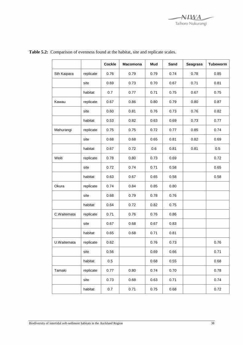
Generally the evenness with which individuals were distributed across species was

greatest at the replicate scale with the least even distribution occurring at the habitat

scale (Table 5.2). Some exceptions to this occurred for all habitat types and for all

locations, with the exception of the Upper Waitemata. In Southern Kaipara, the

habitat scale exhibited greatest evenness for the Sand habitat and moderate evenness

for the Cockle and Macomona habitats. Greatest evenness occurred at the site and

habitat scale for the Sand habitat in Mahurangi, at the habitat scale for the Mud habitat

in Whitford, and at the site scale for the Seagrass habitat in Tamaki. Greater evenness

was also found for the habitat scale rather than the site scale for the Mud habitat in

Okura and Central Waitemata, for the Macomona habitat in Kawau, Mahurangi and

Whitford, and for the Tubeworm habitat in Tamaki.


Table 5.2: Comparison of evenness found at the habitat, site and replicate scales.


Sth Kaipara replicate 0.76 0.79 0.79 0.74 0.78 0.85

site 0.69 0.73 0.70 0.67 0.71 0.81

habitat 0.7 0.77 0.71 0.75 0.67 0.75

Kawau replicate 0.67 0.86 0.80 0.79 0.80 0.87

site 0.60 0.81 0.76 0.73 0.76 0.82

habitat 0.53 0.82 0.63 0.69 0.73 0.77

Mahurangi replicate 0.75 0.75 0.72 0.77 0.85 0.74

site 0.68 0.68 0.65 0.81 0.82 0.69

habitat 0.67 0.72 0.6 0.81 0.81 0.5

Weiti replicate 0.78 0.80 0.73 0.69 0.72

site 0.72 0.74 0.71 0.58 0.65

habitat 0.63 0.67 0.65 0.58 0.58

Okura replicate 0.74 0.84 0.85 0.80

site 0.68 0.79 0.78 0.76

habitat 0.64 0.72 0.82 0.75

C.Waitemata replicate 0.71 0.76 0.76 0.86

site 0.67 0.68 0.67 0.83

habitat 0.65 0.68 0.71 0.81

U.Waitemata replicate 0.62 0.76 0.73 0.76

site 0.56 0.69 0.66 0.71

habitat 0.5 0.68 0.55 0.68

Tamaki replicate 0.77 0.80 0.74 0.70 0.78

site 0.73 0.68 0.63 0.71 0.74

habitat 0.7 0.71 0.75 0.68 0.72



Whitford replicate 0.71 0.86 0.84 0.89 0.79 0.77

site 0.64 0.80 0.77 0.84 0.84 0.72

habitat 0.62 0.7 0.71 0.7 0.77 0.73


6. Summary of results

6.1 Patterns apparent at the replicate core scale

Alpha diversity (i.e., the average number of species per core) showed no strong

patterns between the habitats that applied across all locations. However, Cockle

habitats were more likely to have a high alpha diversity, closely followed by Seagrass

and Tubeworm habitats. Importantly, the habitats described by sediment

characteristics (as mud and sand) were most likely to have a low alpha diversity.

Shannon Weiner and Simpson indices were even less likely to show consistent

patterns across locations, in terms of ranking the habitats. The Cockle habitat was

ranked highest for Shannon-Weiner diversity three times (Weiti Estuary, Upper

Waitemata and Whitford). The Macomona and Sand habitats were both ranked

highest for Shannon-Weiner diversity twice, but the Macomona habitat was also

ranked lowest once and the Sand habitat was ranked lowest in all locations but

Mahurangi and Central Waitemata. The only habitat that never exhibited a high

ranking for Shannon-Weiner diversity was the Mud habitat. For the Simpson index,

the Tubeworm, Cockle and Sand habitats ranked highest in 2 locations each, they each

also ranked lowest in 2 locations. Even the Mud habitat ranked second highest in one

location (Tamaki Strait).

Very few differences were observed in the average number of individuals found in a

replicate, due mainly to high variability in all habitats and locations. Generally the

Tubeworm habitat exhibited the greatest evenness. Interestingly, the Cockle habitat

was the only habitat that never exhibited the highest evenness.

6.2 Diversity at the habitat scale

Gamma diversity (i.e., the total number of species predicted to be found in a habitat if

100 samples were collected) also showed no consistent patterns between the habitats

across locations. The Tubeworm and Cockle habitats were most likely to have high

gamma diversity, while the Mud habitat most frequently had the lowest gamma

diversity.

The differences we observe between the replicate and habitat scale in which habitats

have more species richness are driven by the within habitat heterogeneity. This is

controlled by the number of infrequently occurring species (beta diversity). The only

consistent pattern between habitats across sites was that the Seagrass habitat never


exhibited the highest or lowest beta diversity. Beta diversity was generally high

(>80% of the total number of species), with very little difference occurring between

locations.

For all habitats in all locations, the greatest gain in number of species occurred when

more sites and/or habitat patches were sampled (Table 5.1). Within sites, the species

found in individual cores varied little for the Cockle habitat in all locations. Other

habitats in the Southern Kaipara and the Sand and Tubeworm habitats in other

locations were likely to have more variation between replicates at a site in the species

found, increasing the proportion of within-site beta diversity.

Generally the evenness with which individuals were distributed across species was

greatest within replicates and this decreased to a less even distribution within sites

with another decrease at the habitat scale.

6.3 Bullet point summary

• No habitat had highest diversity across all locations.

• Cockle habitats were most likely to have highest average number of species at

a site, closely followed by Seagrass and Tubeworm habitats.

• Mud habitats were most likely to have low Shannon Weiner and Simpson

indices.

• The Tubeworm habitat was most likely to have high evenness.

• The Tubeworm and Cockle habitats were most likely to have highest predicted

number of species, while the Mud habitat most frequently had the lowest.

• The Seagrass habitat never exhibited the highest or lowest beta diversity.

• Beta diversity was generally high (>80% of the total number of species), with

very little difference occurring between locations. The greatest gain in number

of species occurred when more habitat patches were sampled.


6.4 Conclusions

At present, conservation and management strategies in New Zealand are focussing on

the allocation of Marine Protected Areas. This task requires some determination of

representativeness versus uniqueness of areas in terms of their biodiversity and

ecology. As little information is generally available with which to select specific

areas, New Zealand has developed a classification based on environmental variables

for offshore areas (Snelder et al. 2006) and a biogeographical classification for both

offshore and coastal areas (Ministry of Fisheries and Department of Conservation

2008). While the role of habitats at a smaller-scale is considered, the main focus of the

classifications is on habitats described by environmental variables (depth and substrate

type) rather than including biotic factors (Ministry of Fisheries and Department of

Conservation 2008).

Our results suggest, however, that some species do provide a habitat for other species

and can, therefore, affect biodiversity. The New Zealand cockle, seagrass and the

mats created by maldanid and polydorid tubeworms all created habitats more likely to

have higher average numbers of species (alpha diversity) than the other habitats.

Cockles and tubeworm mats also created habitats likely to have higher total numbers

of species (gamma diversity). Our results are consistent with other published data.

For example, Macomona has been demonstrated to have a negative effect on a

number of species (Thrush et al. 2006b, Thrush et al. 1992). Similarly we did not find

this habitat to have high species richness. Seagrass is internationally considered to be

a habitat of high biodiversity. However similar to our findings, published New

Zealand studies show variable results. Henriques (1980) showed that seagrass habitats

in the Manukau Harbour had higher species diversity than comparable non-vegetated

habitat. Turner et al. (1999) did not always find greater diversity and number of

species inside seagrass patches than on bare sandflats. Alfaro (2006) found higher

average species richness in seagrass than in coarse sand, channels, mud, mangroves, or

pneumatophore zones.

Effects of habitat-creating species in soft sediments, however, go beyond that of

simply affecting biodiversity of the sediment. Effects on oxygen and nutrient fluxes

have been demonstrated for both cockles and Macomona (Thrush et al. 2006b).

Cockles have also been demonstrated to affect benthic-pelagic coupling, with their

feeding changing sedimentation rates (Hewitt & Norkko 2007). Pawson (2004)

suggested that feeding by cockles controlled the availability of food in the water

column (as algal biomass) in Papanui Inlet on the Otago Peninsula. Sandwell (2006)

observed that Macomona feeding and movement destabilised the sediment. Seagrass

habitats have been demonstrated to trap sediment (Larkum et al. 2006, Matheson et al.

2008); polydorid tubeworm mats were observed to stabilise sediment (Thrush et al.


1996). Furthermore, tubeworms, Macomona and cockles are a food source for fish

and birds.

Location-specific variables rather than regional species pools seemed to be most

important for controlling the effect of the relationship between a habitat and its

biodiversity. The Southern Kaipara did not give results that were markedly different

to the other locations, nor did locations spatially close to each other produce results

that were more similar than locations further apart. While local hydrodynamics and

anthropogenic activities are the factors most likely to affect the biodiversity of a

specific habitat, factors such as patch size and density are also likely to be important.

For the Tubeworm habitat, species of tubeworm may also be important; unfortunately

there was not enough information to be able to analysis the relative importance of this

factor. For the seagrass habitat, the presence of other species may also be important.

For example, many of the seagrass sites in the Southern Kaipara contained high

numbers of cockles or tubeworms.

In particular, this report highlights the need to preserve a variety of habitats rather than

concentrate on those that are considered to be of high biodiversity. Indeed preserving

habitat diversity at a variety of scales is likely to be the key to conserving biodiversity

and ecosystem function (Thrush & Dayton 2002, Thrush et al. 2006a).

7. Acknowledgements

Without the data produced by the ARC this report could not have been written.

Thanks also go to James Dare for dataset preparation.


8. References

Alfaro, A.C. (2006). Benthic macro-invertebrate community composition within a mangrove / seagrass estuary in northern New Zealand. Estuarine, Coastal and Shelf Science 66: 97-110.

Berkenbusch, K.; Rowden, A.A. (2007). An examination of the spatial and temporal generality of the influence of ecosystem engineers on the composition of associated assemblages. Aquatic Ecology 41: 129-147.

Clarke, R.T.; Gorley, R.N. (2006). Primer v6. PrimerE, Plymouth.

Colwell, R.K. & Coddington, J.A. (1994). Estimating terrestrial biodiversity through extrapolation. Philosophical Transactions of the Royal Society of London 345: 101-118.

Colwell, R.K. (2006). EstimateS: Biodiversity estimation. 8.0. http://viceroy.eeb.uconn.edu/EstimateS,

Crist, T.O.; Veech, J.A.; Gering, J.C.; Summerville, K.S. (2003). Partitioning species diversity across landscapes and regions: a hierarchical analysis of α, β, and γ diversity. American Naturalist 162: 734-743.

Cummings, V.J.; Pridmore, R.D.; Thrush, S.F.; Hewitt, J.E. (1993). Emergence and floating behaviours of post-settlement juveniles of Macomona liliana (Bivalvia: Tellinacea). Marine Behaviour and Physiology 24: 25-32.

Ellingsen, K.E.; Hewitt, J.E.; Thrush, S.F. (2007). Rare species, habitat diversity and functional redundancy in marine benthos. Journal of Sea Research 58: 291-301.

Henriques, P.R. (1980). Faunal community structure of eight soft shore, intertidal habitats in the Manukau harbour. New Zealand Journal of Ecology 3: 97-103.

Hewitt, J.E.; Norkko, J. (2007). Incorporating temporal variability of stressors into studies: An example using suspension-feeding bivalves and elevated suspended sediment concentrations. Journal of Experimental Marine Biology and Ecology 341: 131-141.

Hewitt, J.E.; Thrush, S.F.; Halliday, J.; Duffy, C. (2005). The importance of small-scale biogenic habitat structure for maintaining beta diversity. Ecology 86: 1618-1626.


Klimek, S.; Marini, L.; Hofman, M.; Isselstein, J. (2008). Additive partitioning of plant diversity with respect to grassland management regime, fertilisation and abiotic factors. Basic and Applied Ecology 9: 626-634.

Lande, R. (1996). Statistics and partitioning of species diversity, and similarity among multiple communities. Oikos 76: 5-13.

Larkum, A.W.D.; Orth, R.J.; Duarte, C.M. (eds) (2006). Seagrasses: Biology, Ecology and Conservation. Dordrecht, The Netherlands. Springer.

Lundquist, C.J.; Vopel, K.; Thrush, S.F.; Swales, A. (2003). Evidence for the physical effects of catchment sediment runoff preserved in estuarine sediments: Phase III macrofaunal communities. NIWA Client Report HAM2003-051 prepared for Auckland Regional Council June 2003. (NIWA Project ARC03202).

MacDiarmid, A. (ed.) (2006). An assessment of biodiversity in the New Zealand marine ecoregion. NIWA Client Report for WWF WLG2006–44. http://www.treasuresofthesea.org.nz/

Matheson, F.; Dos Santos, V.; Pilditch, C. (2008). Environmental stressors of New Zealand seagrass: an introduction and progress report. NIWA Client Report #HAM2008-053 prepared for the Department of Conservation, project #DOC08202.

Ministry of Fisheries, Department of Conservation (2008). Marine protected areas: Classification, protection standard and implementation guidelines. 54 p.

Pawson, M.M. (2004). The cockle Austrovenus stutchburyi and chlorophyll depletion in a southern New Zealand inlet. University of Otago, Dunedin. p.

Pridmore, R.D.; Thrush, S.F.; Hewitt, J.E.; Roper, D.S. (1990). Macrobenthic community composition of six intertidal sandflats in Manukau Harbour, New Zealand. New Zealand Journal of Marine and Freshwater Research 24: 81-96.

Snelder, T.H.; Leathwick, J.R.; Dey, K.L.; Rowden, A.A.; Weatherhead, M.A.; Fenwick, G.D.; Francis, M.P.; Gorman, R.M.; Grieve, J.M.; Hadfield, M.G. (et al.) (2006). Development of anecologic marine classification in the New Zealand region. Environmental Management 39(1): 12-29.

Ricotta, C. (2008). Computing additive diversity from presence-absence scores: a critique and alternative parameters. Theoretical Population Biology 73: 244-249.


Rowden, A.A.; Berkenbusch, K.; Brewin, P.E.; Dalen, J.; Neill, K.F.; Nelson, W.A.; Oliver, M.D.; Probert, P.K.; Schwarz, A-M.; Sui, P.H.; Sutherland, D. (2007). A review of the marine soft-sediment assemblages of New Zealand. NZ Aquatic Environment and Biodiversity Report. 184 pp.

Sandwell, D.R. (2006). Austrovenus stutchburyi, regulators of estuarine benthic-pelagic coupling. University of Waikato, Hamilton. p.

Thrush, S.F.; Gray, J.S.; Hewitt, J.E.; Ugland, K.I. (2006a). Predicting the effects of habitat homogenization on marine biodiversity. Ecological Applications 16: 1636-1642.

Thrush, S.F.; Whitlatch, R.B.; Pridmore, R.D.; Hewitt, J.E.; Cummings, V.J.; Maskery, M. (1996). Scale-dependent recolonization: the role of sediment stability in a dynamic sandflat habitat. Ecology 77: 2472-2487.

Thrush, S.F.; Hewitt, J.E.; Gibb, M.; Lundquist, C.; Norkko, A. (2006b). Functional role of large organisms in intertidal communities: Community effects and ecosystem function. Ecosystems 9: 1029-1040.

Thrush, S.F.; Pridmore, R.D.; Hewitt, J.E.; Cummings, V.J. (1992). Adult infauna as facilitators of colonization on intertidal sandflats. Journal of Experimental Marine Biology and Ecology 159: 253-265.

Thrush, S.F.; Dayton, P.K. (2002). Disturbance to marine benthic habitats by trawling and dredging - Implications for marine biodiversity. Annual Review of Ecology and Systematics 33: 449-473.

Turner, S.J.; Hewitt, J.E.; Wilkinson, M.R.; Morrisey, D.J.; Thrush, S.F.; Cummings, V.J.; Funnell, G. (1999). Seagrass patches and landscapes: the influence of wind-wave dynamics and hierarchical arrangements of spatial structure on macrofaunal seagrass communities. Estuaries 22: 1016-1032.

Ugland, K.I.; Gray, J.S. & Ellingsen, K.E. (2003). The species-accumulation curve and estimation of species richness. Journal of Animal Ecology 72:888-897.


van Houte-Howes, K.S.; Turner, S.J.; Pilditch, C.A. (2004). Spatial differences in Macroinvertebrate communities in intertidal seagrass habitats and unvegetated sediment in three New Zealand estuaries. Estuaries 27: 945-957.

Whittaker, R.H. (1960). Vegetation of the Siskiyou Mountains, Oregon and California. Ecological Monographs 30: 279-338.

biodiversity of intertidal soft-sediment habitats in the ......biodiversity of intertidal...

Documents