biodiversity and the tourism value of changbai …60663/uq60663_oa.pdf · an important...

Tourism Economics, 2000, 6 (4 ), 335–357

Biodiversity and the tourism value ofChangbai Mountain Biosphere Reserve,

China: a Travel Cost approach

D AYUAN X UE, A VERIL C OOK AND C LEM T ISDELL

The Department of Economics, The University of Queensland, Brisbane, Queensland 4072,Australia. Tel: +61 7 3365 6570. Fax: +61 7 3365 7299.

Email: [email protected]

The recreational value of an outdoor site is reflected in a visitor’swillingness to pay for the visit. This can sometimes be estimatedusing the Travel Cost Methodology (TCM) as the consumer surplusunder the site demand curve. Based on a case study of ChangbaiMountain Biosphere Reserve (CMBR) located in Northeast China,this paper focuses on the recreational values of tourism using theTCM and speculates on the extent to which this value depends onthe biodiversity present in CMBR.

Application of the Travel Cost Methodology (TCM ) to value protected areas andoutdoor recreational sites has now become relatively common in Western coun-tries. But, apart from initial research undertaken by Xue1 for Changbai Moun-tain Biosphere Reserve (CMBR ) located in Northeast China, there have beenno such studies for China. The purpose of this paper is to use Xue’s data toestimate the recreational tourism value of CMBR using the TCM and tospeculate on the extent to which this value depends on the biodiversity presentin CMBR.

Considerable gaps exist in our knowledge about the value of biodiversity asa magnet for tourism, even though biodiversity valuation has been designed asa key part of studies of countries by the United Nations Environment Pro-gramme (UNEP).2 Generally, biodiversity in a nature reserve has four categoriesof values: the direct value of extractive goods, the direct value of non-extractiveservices, the indirect value of ecological functions, and non-use values includingexistence value, bequest value and option value.3 A nature reserve is an import-ant facility for conserving biodiversity as well as a resort location for tourism.Recreational value is one of the non-extractive services of biodiversity, and isan important characteristic for a nature reserve.

Helpful comments by Jackie Robinson on an earlier version of this paper are thankfully acknowl-edged. The usual caveat applies.

TOURISM ECONOMICS336

Using the TCM, this article highlights the substantial economic value ofCBMR for tourism, a value believed to depend largely but not exclusively onits conservation of biodiversity. This biodiversity is characterized by the extentof the variety and the number of relatively unique species and ecosystems there.As yet no satisfactory means have been devised or applied to value these variouscharacteristics or attributes as variables. Instead, particular protected areas,species or ecosystems have been valued. A characteristics-type approach, as, forexample, that pioneered by Lancaster,4 may have potential for determining theimportance of various attributes of biodiversity as generators of tourism demand.This is not used here, but it is noted as a gap in current tourism analyses ofthe value of nature conservation. Site valuation using the TCM is undertakenand information is reported which suggests that most of the tourism value ofCMBR is attributable to the biodiversity characteristics present.

The TCM has been applied in many US governmental institutions and itrevealed that the average outdoor recreational value for one person-day in thecountry was US$34 in 1987.5 A study funded by the UK National ForestryCommission evaluated the recreational values of 900,000 ha of six forests underthe Commission by the TCM and the result indicated that the total recreationalvalues in 1988 were up to £53 million.6 Another study reveals that the wildlifeattributes of each forest are estimated to contribute about 38% of the totalrecreational value.7 The TCM is usually used to value a given site, such as inthe study on Achray Forest in the middle of Scotland.8 The method can alsobe used to value a group of sites. Examples are the study of lakes in easternTexas,9 and studies on recreational lakes in the USA.10 Tobias and Mendelsohn11

used the TCM to measure the value of ecotourism at Monteverde Cloud ForestReserve in Costa Rica. They found domestic recreational visits alone representedan annual value of between US$97,500 and $116,200, and foreign visitationrepresented an additional US$400,000 to $500,000 annually.

Description of study site

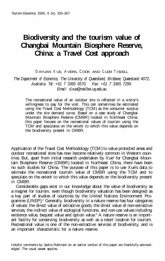
The Changbai Mountains are situated in the northeast of China, straddling theborder with North Korea. Their location is shown in Figure 1.

The CMBR is a typical example of an intact primary natural forest ecosystem.It is a rare natural protected area and includes the highest mountain in north-east China, Bai Yun. This is a volcano, 2,691 metres high with a large and deepcrater lake at the summit that is actually half in North Korea and half in China.CMBR is an attractive recreational site covered by ancestral forests and thou-sands of hot springs, and displays typical altitude vegetation zones in a tem-perate climate, as well as alpine tundra in the far east. CMBR is important forscience and evolution, not only because of the variety of forest types, but alsobecause of its rare fauna and flora and special volcanic relics. There are over 300species of vertebrate animals as well as more than a thousand species of plantsfor medicinal use, many of which are valuable Chinese herbal ingredients.12

Since the reserve opened the north slope of Baitou Peak for tourism in 1982,visitation has increased. There are now around 200,000 people visiting per yearand the total visitor numbers up to 1996 amounted to 1.6 million, of whichmany were from abroad. CMBR was established in 1960 and was incorporated

337Biodiversity and the tourism value of Changbai Mountain Biosphere Reserve, China

Figure 1. The Changbai Mountain Biosphere Reserve in northeast China, onthe border with North Korea.

in the World Biosphere Reserve Network in 1980. Each Biosphere Reserve inthe Network fulfils three basic functions, which are complementary and mu-tually reinforcing:

� a conservation function – to contribute to the conservation of landscapes,ecosystems, species and genetic variation;

� a development function – to foster economic and human development whichis socio-culturally and ecologically sustainable;

� a logistic function – to provide support for research, monitoring, educationand information exchange related to local, national and global issues ofconservation and development.13

The CMBR therefore has as one of its aims the conservation of the biodiversityof the forest ecosystems. This biodiversity has an important direct non-extractiveservice value for science, culture and recreation, as well as remarkable indirectvalues in ecological functions and non-use values such as existence, bequest andoption values. This paper aims to reveal the non-extractive value of domestic


tourism through a case study in CMBR and attempts to evaluate what portionof this value can be attributed to the biodiversity qualities of the reserve.Although international tourism has value, it is not easy to measure using thismethodology, so we concentrate on domestic tourism here.

Description of the economic valuation methodology

The transaction price for most goods can be considered to be an expression ofwillingness to pay for the right to consume the good, or the utility receivedfrom it.

A financial analysis focuses on such market prices and cash flows. However,an economic analysis is concerned with the total value to the whole communityor country including, for example, the existence value of a park or forest thatprovides enjoyment and pleasure to those who visit. It is important in economicsto acknowledge that utility and welfare can be obtained from goods and serviceseven if they are provided free or at minimum charge. The difference betweenthe amount paid and the total utility enjoyed is sometimes measured by the‘consumer surplus’, or CS.

Travel Cost methodology

In this study, the ‘Zonal Travel Cost Method’ is used to measure the recreationalvalue in terms of the economic welfare measure, the consumer surplus. This isa measure of visitors’ willingness to pay for the recreation above the pricecurrently charged. This is a minimum valuation of the site, as it does notinclude the non-use values or the extractive use values.

In order to estimate a value for the recreational use of Changbai MountainBiosphere Reserve, a demand curve is needed. It is not possible to estimate ademand curve directly for the site since there is no variation in the price ofadmission. Only one point on the demand curve can be obtained correspondingto the present entry fee. The TCM enables a demand curve to be derived fordifferent entry fees, based on the actual costs involved for travel to the site. Thisis achieved in a two-step procedure. Once the site demand curve (stage II ) hasbeen estimated then the calculation of consumer surplus can be obtained.

The TCM relies on the assumption that the value people place on the siteis represented by the amount they are willing to pay to travel to it. Thus linkingvisitation rates with travel costs and other socio-economic variables enables itsrecreation value to be estimated. This constitutes stage I of the procedure. Then,assuming that visitors would respond to an increase in entrance fees in the sameway they respond to an increase in travel costs, the second-stage demand curvefor the actual site can be estimated.

Following the methodology initially described by Clawson and Knetsch,14 thewhole country was divided into 37 residential zones by administrative areas,including 28 provincial areas, and 9 municipal areas within Jilin Province,where the reserve is located. The average income for each zone is known, as wellas the distance to the reserve. The statistical data for all residential zones areshown in Table 1. The average travel cost and time taken from each zone canbe calculated. Using this aggregate data the first-stage demand estimation can


be made, which provides an indication of how demand for the reserve variesas the characteristics of the zones vary. Clawson and Knetsch15 call this ‘thedemand curve for the whole recreation experience’. The second stage of thedemand estimation derives a demand curve for the recreation site (CMBR ) itself.The number of visitors at the present entry fee is one point on the demand curvefor the site. In order to derive other points, the travel cost was incremented byvarious amounts and the number of visitors calculated. This was carried out foreach individual zone until visitation from the zone was depressed to zero. Thetotal visitation was then calculated by summing across all the zones for eachincrement. Since the zones at different distances do not exhibit a uniform changein demand for each incremental cost, the resulting relationship between theincremental amounts and total visitation is usually a decreasing non-linearfunction which is called the demand curve for the actual site (or site demandfunction ). This is the second stage of the TCM and assumes that visitors wouldreact to higher entrance fees in the same way they do to higher travel costs.Using the estimated site demand function the consumer surplus can be calcu-lated as the area under the curve above the current costs. This is illustrated inFigure 2, in which DD represents the demand curve and P

1 the current price

paid.It is expected that zones closer to the site, which have lower travel costs and

hence usually higher rates of visitation, will exhibit a more rapid decrease indemand as the cost is incremented. This is because the amount of the incrementconstitutes a larger proportion of travel costs than for those visitors from a moredistant zone.

Calculation of the dependent variable, visitation rate

On-site questioning of 3,131 visitors identified their zonal origin, from whichthe dependent variable in the regression was calculated. The period used wasthe full year 1996. Table A1 in the Appendix indicates that total domesticvisitation for the year amounted to 176,000 people. Assuming the same pro-portion as in the sample, the total number of visitors per residential zone (V

i)

for 1996 can be calculated. This can be used as the dependent variable, oralternatively can be divided by the population for each zone to obtain the visitrate from each zone. Here the zonal visit rate (VR

i) has been calculated by

dividing by the population in tens of thousands, resulting in a rate per tenthousand population.

total number of visitors per residential zone = sample proportion × totalvisitation

ni

Vi = ––––– × 176,000

3,131

total visitors per zonevisit rate from each residential zone = ––––––––––––––––––––

100 × zonal population V

iVRi = ––––––––

100 × ni


Figure 2. Consumer surplus.

Description of independent variables

The most important independent variable is the total travel cost. Travel timewas also considered, as was the average zonal income.

Calculation of total travel costs. The zonal total travel costs include the followingthree items:

� transportation costs based on the actual ticket prices in the summer of 1996for a round-trip by train and bus;

� accommodation costs calculated by trip days multiplied by average standardaccommodation hotel costs plus food; and

� entrance costs – the actual fees (50 yuan per person ) charged by the reserveadministration.

The details of these costs are shown in Appendix Table A1.

Zonal average income. The average annual per capita wages for formal employeesfrom the cities and provinces16 are shown in Table 1. It is noted that thesestatistics are official wages and do not necessarily represent the full income.

It can be seen from Table 1 that the travel costs from some of the zonesconstitute a large proportion of the annual average wage rate for the region. Intwo-thirds of the zones the travel costs are over 25% of the annual salary andin one-quarter of the zones they are more than 40% of the annual salary. It isunreasonable to assume that people earning only the average wage would spendthis much on a short holiday. The visitors to this special Biosphere Reserve arelikely to earn well above the zonal average, and so have far more discretionary


income than the common worker. Many visitors also are entitled to reimburse-ment for their visitation expenditures. Hence, the assumption that the visitors’incomes are representative of the zonal population average incomes may not beapplicable.

Consideration of travel time. Incorporating travel time into a travel cost analysishas received wide attention. Visitors from distant zones visit the site lessfrequently than those who live closer, because of the combined effect of trans-portation costs and travel time. The opportunity cost of scarce time acts as aseparate deterrent at the margin to visiting more distant sites.17 Failure toinclude travel time will bias the results. In 1987 the UK Department ofTransport, in a re-appraisal of the value of non-working time, advocated astandard average appraisal value of 43% of earnings, with slightly higher valuesfor adults and people of working age, but a lower value for retired people andchildren. This amount is used by Willis and Benson18 to value non-working orleisure time forgone to visit the forest sites. Chavas et al19 consider that theopportunity value of travel time is between 30% and 50% of actual wage. ButSmith et al20 assume that the opportunity cost of time is equal to the wage rate,and they find that assuming a fraction of the opportunity cost is not superiorto using the full wage rate. In this study, travel time has been arbitrarily valuedat 40% of the average wage for each zone for the travel time involved.

Travel time and travel cost cannot both be included in a regression analysis,as discussed. Estimation has been carried out in this study in two ways: (a ) usingonly travel costs (TC) and (b) using travel costs plus travel time (TT) (but noton-site time ) valued at 40% of the wage rate. On-site time has been consideredto be a benefit rather than a cost, since CMBR is taken as a single destinationtrip.

The travel time opportunity cost has been calculated as follows:

total work hours per year = No of working days × average workday hours

= 254 × 8

= 2,032 hours

average wage per year average zonal hourly wage per person = ––––––––––––––––––– × 40% 2,032

total travel hours = hours by train or bus + hours for transit + on-site time(as shown in Table 1, column 3 )

value of travel time per person = (total travel hours – 36 ) × average hourlywage

Since on-site time has not been included in the travel cost analysis and visitors,on average, spend one night and two days at the Reserve, 36 hours have beendeducted from the total travel hours.


Table 1. Sampling data statistics and visiting rates of residential zones.

Residential zones Population 1995 avge Total Total Sampling 1996 Visitingin 1995 wage travel cost number visiting rate(million ) (yuan/per time (yuan/ (persons ) quantity to CMBR

capita) (hours ) trip ) to CMBR in 1996(trips ) (o/000 )

Changcun, Jilin Prov. 6.78 5,119 79 573 494 27,773 40.96Jilin, Jilin Prov. 4.34 4,635 74 514 301 16,914 38.97Siping, Jilin Prov. 3.15 3,562 71 551 66 3,714 11.79Liaoyuan, Jilin Prov 1.25 3,649 68 498 60 3,379 27.03Tonghua, Jilin Prov. 2.28 4,026 48 385 161 9,046 39.68Baishan, Jilin Prov. 1.32 3,781 45 357 286 16,069 121.73Songyuan,Jilin Prov 2.59 4,338 103 722 37 2,077 8.02Baicheng, Jilin Prov 1.99 3,303 110 808 19 1,074 5.40Yanbian, Jilin Prov. 2.22 4,030 48 330 595 33,446 150.66Heilongjiang Prov. 37.01 4,145 99 752 272 15,294 4.13Liaoning Prov. 40.92 4,911 87 617 297 16,695 4.08Beijing Munic. 12.51 8,144 124 1,158 275 15,458 12.36Tianjin Munic. 9.42 6,501 120 1,094 39 2,200 2.34Hebei Prov. 63.47 4,839 144 1,352 17 950 0.15Shanxi Prov. 30.77 4,721 151 1,457 6 334 0.11Inner-Mongolia Reg. 22.84 4,134 156 1,526 7 387 0.17Shandong Prov. 87.05 5,145 131 1,257 50 2,811 0.32Shanghai Munic. 14.15 9,279 158 1,688 14 787 0.56Jiangsu Prov. 70.66 5,943 150 1,554 27 1,518 0.21Zhejiang Prov. 43.17 6,619 188 1,862 7 387 0.09Anhui Prov. 60.13 4,609 172 1,620 3 176 0.03Fujian Prov. 32.37 5,857 216 2,299 3 176 0.05Jiangxi Prov. 40.63 4,211 206 2,145 1 53 0.01Henan Prov. 91.00 4,344 168 1,557 31 1,742 0.19Hubei Prov. 57.72 4,685 183 1,795 5 282 0.05Hunan Prov. 63.92 4,797 194 1,958 3 176 0.03Guangdong Prov. 68.68 8,250 215 2,284 28 1,566 0.23Guangxi Reg. 45.43 5,105 222 2,397 5 282 0.06Hainan Prov. 7.24 5,340 248 2,627 1 53 0.07Sichuan Prov. 113.25 4,645 207 2,162 8 458 0.04Guizhou Prov. 35.08 4,475 221 2,383 4 229 0.07Yunnan Prov. 39.90 5,149 239 2,671 1 53 0.01Shaanxi Prov. 35.14 4,396 182 1,769 2 106 0.03Gansu Prov. 24.38 5,493 200 2,116 4 229 0.09Qinghai Prov. 4.81 5,753 208 2,186 1 53 0.11Xinjiang Reg. 16.61 5,348 256 2,937 1 53 0.03Tibet Reg. 2.40 7,382 328 3,444 0 0 0

Analysis of recreational value

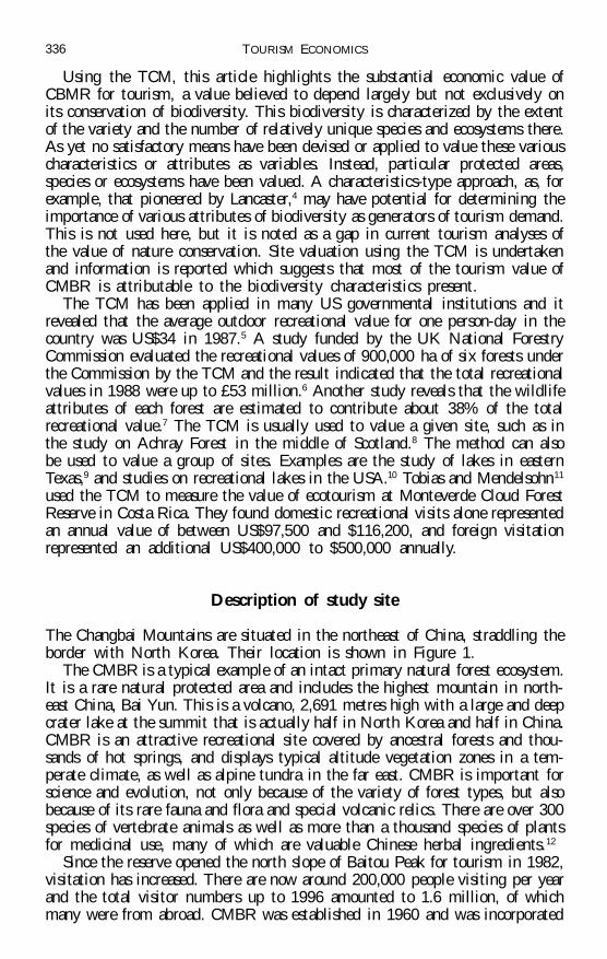
Travel cost stage I regressionThe first-stage regression relates visitation rates to travel cost and other vari-ables. The data for the CMBR include total population, travel cost, and traveltime. It can be seen from the correlation matrix in Table 2 that there is almost


Table 2. Correlation matrix of variables.

Visit rate Number of Average wage Travel cost Travel timeVR visitors V Y TC t

Visit rate 1Visiting quantity 0.767296 1Average wage –0.28102 –0.14223 1Travel cost –0.54871 –0.64931 0.419691 1Travel time –0.58715 –0.66107 0.405316 0.993555 1

perfect correlation between the travel cost and travel time. Hence, both variablescannot be included in the regression as the estimation would have almost perfectmulticollinearity.

There is a low correlation between each of the possible dependent variables(V, VR ) and the average zonal wage, which again suggests that the visitors toCMBR are not the ‘average’ for the zone in terms of wages.

Since only zonal averages for income and travel distance and time are avail-able, it is necessary to build an aggregate travel cost model. This can providean indication of how demand for the reserve varies as the characteristics of thezones vary. However, there are limitations to using aggregate data. Hellerstein21

points out that, if only averages and sums are available, then only linear modelscan be estimated consistently. If additional information on the distribution ofthe aggregate data is available, then the set of models can be expanded toinclude non-linear functional forms. These data are not available in this case.

Linear initial regressions. When linear regressions were estimated (taking intoaccount Hellerstein’s warning ) none were particularly satisfactory. Average in-come was not a significant variable when included in a multiple regression witheither travel costs or travel costs plus time, as shown in Table 3 in which t valuesare shown in parentheses.

Non-linear initial regressions. Non-linear estimation produced a much better fitto the data, as shown in Table 4. In both the linear and non-linear estimations,it can be seen that the inclusion of the value of travel time does not improvethe estimation, with the first equation in each of the above tables giving thebest fit. Durbin–Watson values of 1.7 indicate no autocorrelation problem forn = 37 and two independent variables.

Travel cost stage II demand curve derivation

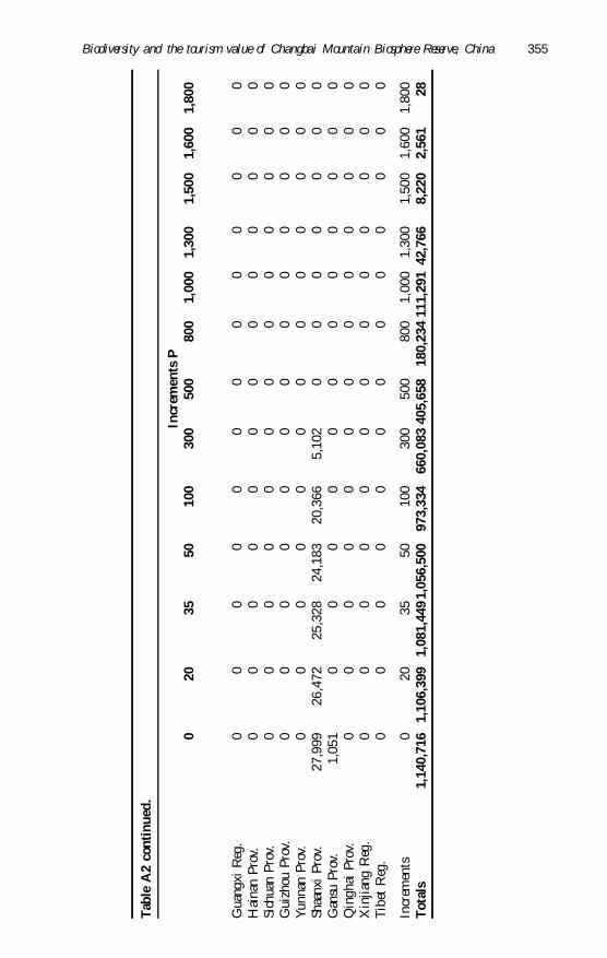
The first regression equation from Table 3, relating visit rates to total travelcost only, and the first equation from Table 4 have been used to derive separatedemand curves for the CMBR (the demand curve for the recreation resource ).Various entry fee levels can be represented by incrementing the travel cost valuesfor each zone until visitation drops to zero.22 For each increment the visitationrate for the zone can be calculated and all the zones summed to obtain the totalvisitation rate at that increment. These values are shown in Appendix TablesA2 and A3. Table A2 shows the estimated visitation rates at various increments


Table 3. Linear regressions estimated.

Regression equation F p-value R2 –R2 D–W

VR = 46.39 – 0.0217TC 15.078 0.00044 0.301 0.281 2.22(4.75 ) (–3.88 )

VR = 45.6 – 0.0197TT 14.96 0.0001 0.300 0.279 2.22(4.74 ) (–3.87 )

VR = 52.38 – 0.00147Y – 0.0207TC 7.43 0.00210 0.304 0.263 2.27 (2.87 ) (–0.39* ) (–3.32 )

VR = 50.06 – 0.001106Y – 0.0190TT 7.33 0.00226 0.301 0.260 2.26 (2.74 ) (–0.289* ) (–3.29 )

TT = travel cost plus value of travel time but not including on-site time* = not significant at 5% levelD–W = Durbin–Watson statistic

Table 4. Non-linear regressions estimated.

Equation F R2 –R2 D–W

ln VR = 8.054 + 2.889lnY – 4.66 lnTC 223 0.93109 0.92691 1.675(1.652* ) (4.54 ) (–20.36 )

ln VR = 5.060 + 3.196lnY – 4.563lnTT 221 0.93044 0.92623 1.704 (1.027* ) (4.94 ) (–20.26 )

VR = 214.5 + 6.26lnY – 35.58lnTC 16.4 0.490 0.460 2.27(1.47* ) (0.325* ) (–5.099 )

ln VR = 3.046 + 0.000328Y – 0.00357TC 80.2 0.82939 0.81905 1.149(3.68 ) (1.97* ) (–12.4 )

TT = travel cost plus value of travel time but not including on-site time* = not significant at 5% levelD–W = Durbin–Watson statisticp-values for the F statistic are not quoted since they are all close to zero

Table 5. Estimated stage II regressions from initial first-stage linear regressions.

Regression equation F R2 –R2 D–W

P = 2940.57 – 194.407lnV 55.0 0.833 0.818 0.612 (9.38 ) (–7.41 )

P = 1370.6 – 0.001302V 87.5 0.888 0.878 0.314(370.62 ) (–9.36 )

ln P = 7.424 – 3.402×10–6 V 261 0.963 0.959 0.636 (54.1 ) (–16.16 )

P = 1526.16 – 0.00321V + 1.703×10–9 V2 128.59 0.963 0.955 0.670(22.17 ) (–7.35 ) (4.45 )

p-values for the F statistic are not quoted since they are all close to zero


above the present entry fee starting from a first-stage linear estimation, whereasTable A3 shows the estimated visitation rate calculated from the initial non-linear first-stage equation.

Stage II estimations and consumer surplus from initial linear regressions. The esti-mated functions connecting the increments (P ) with the estimated total numberof visitors (V ) (for linear initial estimation ) are shown in Table 5. From the tableit can be seen that the log-linear form and the quadratic form of the demandcurve give similar statistics and appear to fit the data better than the first twoequations estimated. However, they both have a problem of autocorrelation, butsince the procedure simply requires integration to find the area under the curve,the presence of autocorrelation does not present difficulty.

It was decided to use the log-linear form for the site demand curve origi-nating from a linear first-stage estimation. The relationship between price (P= increment ) and quantity (V = number of visitors ) is therefore:

P = e7.424 e–0.000003402 V = 1674.93 e–0.000003402 V.

This estimated demand curve and the total demand (from Appendix Table A2)are plotted in Figure 3.

The consumer surplus is calculated as the area under this curve in the firstquadrant. Since the increments are plotted against the estimated total visitation,this is the area above the present entry price.

The consumer surplus, or area under the function, is:

1.2m e–00.000003402× 1.2m – 1 1674.93e–0.000003402 VdV = 1674.93 ––––––––––––––

0 –0.000003402

= 492336860.7[ e–4.0824 – 1]

= 48.4 m yuan

Stage II estimations and consumer surplus from initial non-linear regressions. Theestimated functions connecting the increments (P ) with the total visitors (V )(for non-linear initial estimation ) are shown in Table 6.

Table 6. Stage II estimation from initial non-linear equation.

Equations F R2 –R2 D–W

P = 1277.2 – 0.023745V + 9.175×10–8 V2 10.8 0.682 0.619 0.378(7.96 ) (–3.49 ) (2.46 ) (0.0032 )

lnP = 7.023 – 2.64×10–5 V 85.5 0.895 0.885 0.281(49.7 ) (–9.25 )

lnP = 11.96 – 0.631lnV 172 0.945 0.939 0.459(27.1 ) (–13.12 )

P = 3918.9 – 339.7 lnV 187 0.944 0.939 0.258(16.7 ) (–13.7 )

p-values for the F statistic are close to zero. The highest value is shown in parentheses and the others areof the order of 10–6 or less.


Figure 3. Demand and estimated demand.

Using the final equation, the consumer surplus may be calculated as follows:

102370 102370

0 3918.9 – 339.7 ln V dV = [3918.9 – 339.7V(ln V – 1 )]

0

= 34.78 m yuan

This value of consumer surplus is much less than the one estimated from aninitial linear regression which was not a particularly good fit to the data eventhough it may have had the property of consistency. This latter, lower value istherefore taken as the minimum measure of the recreation value of CMBR andis used later in the paper.

The estimated demand function P = 3918.9 – 339.7 lnV and the totaldemand from Appendix Table A3 are plotted in Figure 4.

Summary of results

Results of valuation

Total travel expenses. By calculation, the total travel costs of all domestic visitorsto CMBR in 1996 was 114.75 million yuan as shown in Appendix Table A1.

Total consumer surplus. The consumer surplus value was found (above ) to be34.78 million yuan.

Total travel time costs. The total value of travel time was calculated to be 8.61million yuan using (travel hours – 36) × average hourly wage × 40% × zonalvisitation numbers to CMBR. The average hourly wage is described earlier andother data are presented in Table 1.


Figure 4. Demand curve and total estimated demand from an initial non-linearestimation.

Other expenses. There are other expenses for visitors, mainly photography, shop-ping for souvenirs, local art and crafts, native products, cultural T-shirts andother items, which reflect the characteristics of the site. A survey showed thateach visitor spent 80 yuan on average for these purchases:

total other expenses = total domestic visitors to CMBR in 1996 × averageexpenses

= 176,000 × 80

= 14.08 million yuan

Total recreational value for domestic tourism:

total recreational = travel + consumer + travel time + other value cost surplus value expenses

= 114.75 + 34.78 + 8.61 + 14.08

= 172.22 (million yuan/year )

Recreational value of biodiversity for CMBR

CMBR is characterized by its rich biodiversity, especially the primary forestecosystem. However, the total recreational value noted above cannot all beattributed to this biodiversity because there are other famous geological and


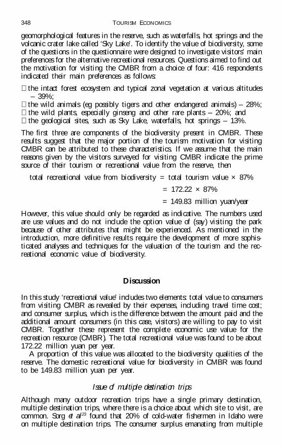
geomorphological features in the reserve, such as waterfalls, hot springs and thevolcanic crater lake called ‘Sky Lake’. To identify the value of biodiversity, someof the questions in the questionnaire were designed to investigate visitors’ mainpreferences for the alternative recreational resources. Questions aimed to find outthe motivation for visiting the CMBR from a choice of four: 416 respondentsindicated their main preferences as follows:

� the intact forest ecosystem and typical zonal vegetation at various altitudes– 39%;

� the wild animals (eg possibly tigers and other endangered animals ) – 28%;� the wild plants, especially ginseng and other rare plants – 20%; and� the geological sites, such as Sky Lake, waterfalls, hot springs – 13%.

The first three are components of the biodiversity present in CMBR. Theseresults suggest that the major portion of the tourism motivation for visitingCMBR can be attributed to these characteristics. If we assume that the mainreasons given by the visitors surveyed for visiting CMBR indicate the primesource of their tourism or recreational value from the reserve, then

total recreational value from biodiversity = total tourism value × 87%

= 172.22 × 87%

= 149.83 million yuan/year

However, this value should only be regarded as indicative. The numbers usedare use values and do not include the option value of (say ) visiting the parkbecause of other attributes that might be experienced. As mentioned in theintroduction, more definitive results require the development of more sophis-ticated analyses and techniques for the valuation of the tourism and the rec-reational economic value of biodiversity.

Discussion

In this study ‘recreational value’ includes two elements: total value to consumersfrom visiting CMBR as revealed by their expenses, including travel time cost;and consumer surplus, which is the difference between the amount paid and theadditional amount consumers (in this case, visitors ) are willing to pay to visitCMBR. Together these represent the complete economic use value for therecreation resource (CMBR ). The total recreational value was found to be about172.22 million yuan per year.

A proportion of this value was allocated to the biodiversity qualities of thereserve. The domestic recreational value for biodiversity in CMBR was foundto be 149.83 million yuan per year.

Issue of multiple destination trips

Although many outdoor recreation trips have a single primary destination,multiple destination trips, where there is a choice about which site to visit, arecommon. Sorg et al23 found that 20% of cold-water fishermen in Idaho wereon multiple destination trips. The consumer surplus emanating from multiple


destination trips is a large component of total site value.24 Sorg et al25 usingthe contingent valuation method, found that multiple destination visitorsactually placed a higher marginal value on the measured recreation site thansingle destination users of that site.

In this study CMBR has no close substitutes, and a visit to the reserve maybe considered as a single destination trip. The multiple destination issue isignored and on-site time has not been included as a cost. Among the 3,131survey respondents, there were 64.5% from Jilin Province in which the reserveis located, 18.2% from Liaoning and Heilongjiang, two neighbouring provincesof Jilin, and 8.8% from Beijing. So 91.5% of visitors can be regarded as havingthe CMBR as their sole destination because there is no other attractive recrea-tional site near the reserve. The other 8.5% of visitors were from more than20 other provinces or regions, and would possibly have other destinations formeetings or recreational visiting. Due to this small proportion, the multipledestination trip issue is not taken into account in this paper.

Recreational value of foreign visitors

CMBR is of international recreational significance, with many foreign visitorsespecially from South Korea. In 1996, the number of foreign visitors was71,312, constituting 28.8% of total visitors. These visitors have higher travelcosts and they generate producer surplus for providers of recreation-relatedproducts and services as well as contributing to consumer surplus. Recreationalvalue for foreign visitors has not been dealt with in this paper. So, actually, theestimate for recreational value calculated on domestic visitors is not the wholerecreational value of the reserve or of biodiversity within the reserve.

Conclusion and comment

This study has found the consumer surplus value for CMBR using the ZonalTravel Cost methodology to be 34.78 million yuan (US $4.2 million ). This isconsidered to be a minimum estimate. The total biodiversity recreational valueof the reserve has been found to be 149.83 million yuan (US $18.2 million).These valuations are for only one year (1996 ) and therefore are static estimates.In the longer term those values can be expected to increase.

The recreational value estimation in China is based mainly on visitors’ travelcosts involving bus and train travel. The availability of public transport isimportant for visitation in China since most people depend on public transpor-tation. When suitable public transport is available to visit a recreation site, ahigher consumer surplus value will be found for biodiversity recreation. Butthose sites that are not easy to access now, or are currently short of tourismfacilities, will display a lower recreational value even if they possess a richbiodiversity. This paper has suggested a biodiversity recreation value for CMBRin 1996. With further development in ecotourism infrastructure, and improve-ments in transportation in the future, this value is likely to increase. With risingincomes in China and more leisure-time as China develops, Chinese demand forrecreation in CMBR can be expected to grow and the tourism value of CMBRto rise. In addition, there is opportunity in the future to evaluate the recreational


value of biodiversity in other more remote sites when ecotourism is betterdeveloped. It follows that current tourism economic values of protected areasin China are likely to understate considerably the long-term recreational valuesof these areas, or the discounted present sum of the future tourism economicvalues of such areas, which far exceeds their current annual recreational economicvalue.26

Endnotes

1. Dayuan Xue, Economic Valuation of Biodiversity - A Case Study on Changbai Mountain BiosphereReserve in Northeast China, China Environmental Sciences Press (Chinese version), Beijing, 1997.

2. UNEP (United Nations Environmental Program), Guidelines for Country Studies on BiologicalDiversity, Oxford University Press, Oxford, 1993.

3. Dayuan Xue, ‘Categories and valuation methods of economic values of biodiversity in naturereserves’, Rural Eco-Environment (Chinese version), Vol 15, No 2, 1999, pp 54-59.

4. K. Lancaster, ‘A new approach to consumer theory’, Journal of Political Economy, Vol 74, 1966,pp 132-137.

5. R.G. Walsh, R.D. Bjonback, R.A. Aiken and D.H. Rosenthal, ‘Estimating the public benefitsof protecting forest quality’, Journal of Environmental Management, Vol 30, 1990, pp 175-189.

6. K.G. Willis and J.F. Benson, ‘A comparison of user benefit and costs of nature conservationat three nature reserves’, Regional Studies, Vol 22, 1988, pp 417-428; Ian Bateman, ‘Placingmoney values on the unpriced benefits of forestry’, Quarterly Journal of Forestry, Vol 86, 1992,pp 9-17.

7. K.G. Willis and J.F. Benson, ‘Recreational value of forests’, Forestry, Vol 62, No 2, 1989, pp93-109.

8. D.N. Hanley, ‘Valuing rural recreation benefits: an empirical comparison of two approaches’,Journal of Agricultural Economics, Vol 40, 1989, pp 361-374.

9. C. Seller, J.R. Stoll and J-P. Chavas, ‘Validation of empirical measures of welfare change: acomparison of non-market techniques’, Land Economics, Vol 61, 1985, pp 156-175.

10. V.K. Smith, W.H. Desvousges and A. Fisher, ‘A comparison of direct and indirect methods forestimating environmental benefits’, American Journal of Agricultural Economics, Vol 68, 1986, pp280-290.

11. D. Tobias and R. Mendelsohn, ‘Valuing ecotourism in a tropical rain-forest reserve’, Ambio, Vol20, No 2, 1991, pp 91-93.

12. http://www.chinarainbow.com/english/lyuyou/zdmsh.htm13. http://www.euromab.org/brprogram/what.html14. Marion Clawson and Jack L. Knetsch, Economics of Outdoor Recreation, Johns Hopkins University

Press, Baltimore, MD, 1966.15. Ibid, at p 61.16. These are taken from the 1996 China Statistics Yearbook (p 117) and the 1996 China Labour

Statistics Yearbook (p 141), China Statistical Publishing House, Beijing.17. Frank A. Ward and John B. Loomis, ‘The Travel Cost Demand Model as an environmental policy

assessment tool: a review of the literature’, Western Journal of Agricultural Economics, Vol 11, No 2,1986, pp 164-178.

18. K.G. Willis and J.F. Benson, ‘A comparison of user benefit and costs of nature conservationat three nature reserves’, Regional Studies, Vol 22, 1988, pp 417-428.

19. J-P. Chavas, J. Stoll and C. Seller, ‘On the commodity value of travel time in recreationalactivities’, Applied Economics, Vol 21, 1989, pp 711-722.

20. V.K. Smith, W.H. Desvousges and A. Fisher, ‘A comparison of direct and indirect methods forestimating environmental benefits’, American Journal of Agricultural Economics, Vol 68, 1986, pp280-290.

21. D. Hellerstein, ‘Welfare estimation using aggregate and individual-observation models: a com-parison using Monte-Carlo techniques’, American Journal of Agricultural Economics, Vol 77, No 3,1995, pp 620-630, at p 621.

22. It is important to keep incrementing until the visitation drops to zero, since otherwise thesummations of the visitation quantity data will be truncated. This may simply result in aninaccurate estimation of the demand function and hence consumer surplus, or else in points


representing only a limited section of the demand curve, making the choice of functional formin the estimation difficult due to extrapolation. This difficulty of finding the correct functionalform due to having only a narrow band of values for the independent variable has occurred inD.J. Beal ‘A travel cost analysis of the value of Carnarvon Gorge National Park for recreationaluse’, Review of Marketing and Agricultural Economics, Vol 63, No 2, 1995, pp 292–303. Beal limitsher increments to a maximum of $20 instead of finding the increment value (or entry fee) forwhich visitation becomes zero.

23. C.J. Sorg et al, ‘Net economic value of cold and warm water fishing in Idaho’, Resource BulletinRM-11, USFS, USDA, 1985.

24. R. Mendelsohn, J. Hof, G. Peterson, and R. Johnson, ‘Measuring recreation values with multipledestination trips’, American Journal of Agricultural Economics, Vol 74, 1992, pp 926-933.

25. Op cit, Ref 23.26. See also C. Tisdell, ‘Investment in ecotourism: assessing its economics’, Tourism Economics, Vol 1,

No 4, 1995, pp 375-387.

Appendix

(see overleaf )

TOURISM ECONOMICS352T

able

A1.

Th

e tr

avel

exp

ense

s to

CM

BR

for

th

e d

omes

tic

visi

tors

.

Reg

ion

Dis

tan

ce t

oT

ran

spor

tF

ood

Acc

omm

.E

ntr

y fe

eT

otal

tra

vel

Tot

al v

isit

orT

otal

Tot

al t

rave

ln

earb

y ci

tyco

stco

stco

st+

ser

vice

cost

sn

um

ber

str

ansp

ort

cost

in

199

6(k

m)

(yu

an/p

)(y

uan

/p)

(yu

an/p

)(y

uan

/p)

(yu

an/p

)in

199

6co

st(m

illi

on(p

eop

le)

(mil

lion

yu

an)

yuan

)

Cha

ngcu

n, J

ilin

Pro

v.47

729

113

210

050

573

27,7

738.

0815

.91

Jili

n, J

ilin

Pro

v.34

924

012

410

050

514

16,9

144.

068.

69Si

ping

, Ji

lin

Pro

v.59

228

112

010

050

551

3,71

41.

042.

05Li

aoyu

an,

Jili

n P

rov.

480

236

112

100

5049

83,

379

0.80

1.68

Tong

hua,

Jil

in P

rov.

277

155

8010

050

385

9,04

61.

403.

48B

aish

an,

Jili

n P

rov.

217

131

7610

050

357

16,0

692.

115.

74So

ngyu

an,

Jilin

Pro

v.62

635

017

215

050

722

2,07

70.

731.

50B

aich

eng,

Jil

in P

rov.

810

424

184

150

5080

81,

074

0.46

0.87

Yan

bian

, Ji

lin

Pro

v.10

080

100

5033

033

,446

3.34

11.0

4H

eilo

ngji

ang

Pro

v.71

938

816

415

050

752

15,2

945.

9311

.50

Liao

ning

Pro

v.63

529

814

412

550

617

16,6

954.

9810

.30

Bei

jing

Mun

ic.

1,62

375

020

815

050

1,15

815

,458

11.5

917

.90

Tia

njin

Mun

ic.

1,48

669

420

015

050

1,09

42,

200

1.53

2.41

Heb

ei P

rov.

1,90

686

224

020

050

1,35

295

00.

821.

28Sh

anxi

Pro

v.2,

137

955

252

200

501,

457

334

0.32

0.49

Inne

r M

ongo

lia

Reg

.2,

291

1,01

626

020

050

1,52

638

70.

390.

59Sh

ando

ng P

rov.

1,84

383

722

015

050

1,25

72,

811

2.35

3.53

Shan

ghai

Mun

ic.

2,81

11,

224

264

150

501,

688

787

0.96

1.33

Jian

gsu

Pro

v.2,

506

1,10

225

215

050

1,55

41,

518

1.67

2.36

Zhe

jian

g P

rov.

3,00

01,

300

312

200

501,

862

387

0.50

0.72

Anh

ui P

rov.

2,45

61,

082

288

200

501,

620

176

0.19

0.29

Fujia

n P

rov.

3,97

21,

689

360

200

502,

299

176

0.30

0.40

Jian

gxi

Pro

v.3,

628

1,55

134

420

050

2,14

55

30.

080.

11H

enan

Pro

v.2,

318

1,02

728

020

050

1,55

71,

742

1.80

2.71

Hub

ei P

rov.

2,85

21,

241

304

200

501,

795

282

0.35

0.51

cont

inue

d


Tab

le A

1 co

nti

nu

ed.

Reg

ion

Dis

tan

ce t

oT

ran

spor

tF

ood

Acc

omm

.E

ntr

y fe

eT

otal

tra

vel

Tot

al v

isit

orT

otal

Tot

al t

rave

ln

earb

y ci

tyco

stco

stco

st+

ser

vice

cost

sn

um

ber

str

ansp

ort

cost

in

199

6(k

m)

(yu

an/p

)(y

uan

/p)

(yu

an/p

)(y

uan

/p)

(yu

an/p

)in

199

6co

st(m

illi

on(p

eop

le)

(mil

lion

yu

an)

yuan

)

Hun

an P

rov.

3,21

01,

384

324

200

501,

958

176

0.24

0.34

Gua

ngdo

ng P

rov.

3,93

61,

674

360

200

502,

284

1,56

62.

623.

58G

uang

xi R

eg.

4,18

81,

775

372

200

502,

397

282

0.50

0.68

Hai

nan

Pro

v.4,

537

1,91

541

225

050

2,62

753

0.10

0.14

Sich

uan

Pro

v.3,

671

1,56

834

420

050

2,16

245

80.

720.

99G

uizh

ou P

rov.

4,16

31,

765

368

200

502,

383

229

0.40

0.55

Yun

nan

Pro

v.4,

802

2,02

140

020

050

2,67

153

0.11

0.14

Shan

xi P

rov.

2,78

81,

215

304

200

501,

769

106

0.13

0.19

Gan

su P

rov.

3,43

61,

474

392

200

502,

116

229

0.34

0.48

Qin

ghai

Pro

v.3,

721

1,58

834

820

050

2,18

653

0.08

0.12

Xin

jian

g R

eg.

5,29

72,

259

428

200

502,

937

530.

120.

16T

ibet

Reg

.5,

711

2,38

456

045

050

3,44

40

00

Tot

al17

6,00

061

.14

114.

75


able

A2.

Est

imat

ed v

isit

atio

n n

um

ber

s u

sin

g V

R =

46.

3904

9 –

0.02

172T

C;

V =

100

Ni V

R.

Incr

emen

ts P

020

3550

100

300

500

800

1,00

01,

300

1,50

01,

600

1,80

0

Cha

ngcu

n, J

ilin

Pro

v.23

,015

22,7

2022

,499

22,2

7821

,542

18,5

9715

,652

11.2

348,

289

3,87

192

50

0Ji

lin,

Jil

in P

rov.

15,2

8815

,100

14,9

5814

,817

14,3

4612

,460

10,5

757,

747

5,86

23,

034

1,14

920

60

Sipi

ng,

Jili

n P

rov.

10,8

4310

,706

10,6

0410

,501

10,1

598,

791

7,42

25,

370

4,00

11,

949

580

00

Liao

yuan

, Ji

lin

Pro

v.4,

447

4,39

24,

352

4,31

14,

175

3,63

23,

089

2,27

51,

732

917

374

103

0To

nghu

a, J

ilin

Pro

v.8,

670

8,57

18,

497

8,42

38,

175

7,18

56,

194

4,70

93,

718

2,23

31,

242

747

0B

aish

an,

Jili

n P

rov.

5,10

05,

043

5,00

04,

957

4,81

34,

240

3,66

62,

806

2,23

31,

373

799

513

0So

ngyu

an,

Jilin

Pro

v.7,

954

7,84

17,

757

7,67

27,

391

6,26

65,

141

3,45

32,

328

640

00

0B

aich

eng,

Jil

in P

rov.

5,73

95,

653

5,58

85,

523

5,30

74,

443

3,57

82,

281

1,41

712

00

00

Yan

bian

, Ji

lin

Pro

v.8,

707

8,61

18,

539

8,46

68,

225

7,26

16,

297

4,85

03,

886

2,43

91,

475

993

28H

eilo

ngji

ang

Pro

v.11

1,24

110

9,63

310

8,42

810

7,22

210

3,20

387

,125

71,0

4846

,933

30,8

556,

740

00

0Li

aoni

ng P

rov.

134,

992

133,

214

131,

881

130,

548

126,

104

108,

329

90,5

5363

,889

46,1

1419

,450

1,67

50

0B

eijin

g M

unic

.26

,570

26,0

2625

,619

25,2

1123

,852

18,4

1812

,984

4,83

20

00

00

Tia

njin

Mun

ic.

21,3

1620

,907

20,6

0020

,293

19,2

7015

,178

11,0

864,

948

856

00

00

Heb

ei P

rov.

108,

058

105,

301

103,

233

101,

165

94,2

7266

,701

39,1

300

00

00

0Sh

anxi

Pro

v.45

,369

44,0

3243

,030

42,0

2738

,685

25,3

1911

,952

00

00

00

Inne

r M

ongo

lia

Reg

.30

,253

29,2

6128

,517

27,7

7325

,292

15,3

715,

449

00

00

00

Shan

dong

Pro

v.16

6,16

516

2,38

415

9,54

715

6,71

114

7,25

810

9,44

371

,629

14,9

070

00

00

Shan

ghai

Mun

ic.

13,7

6413

,149

12,6

8812

,227

10,6

914,

544

00

00

00

0Ji

angs

u P

rov.

89,2

9786

,228

83,9

2681

,624

73,9

5043

,255

12,5

610

00

00

0Z

heji

ang

Pro

v.25

,677

23,8

0222

,395

20,9

8916

,300

00

00

00

00

Anh

ui P

rov.

67,3

7064

,758

62,7

9960

,840

54,3

1028

,189

2,06

90

00

00

0Fu

jian

Pro

v.0

00

00

00

00

00

00

Jian

gxi

Pro

v.0

00

00

00

00

00

00

Hen

an P

rov.

114,

409

110,

456

107,

491

104,

527

94,6

4455

,114

15,5

830

00

00

0H

ubei

Pro

v.42

,731

40,2

2338

,343

36,4

6230

,194

5,12

00

00

00

00

Hun

an P

rov.

24,6

9121

,914

19,8

3117

,749

10,8

070

00

00

00

0G

uang

dong

Pro

v.0

00

00

00

00

00

00

cont

inue

d


Tab

le A

2 co

nti

nu

ed.

Incr

emen

ts P

020

3550

100

300

500

800

1,00

01,

300

1,50

01,

600

1,80

0

Gua

ngxi

Reg

.0

00

00

00

00

00

00

Hai

nan

Pro

v.0

00

00

00

00

00

00

Sich

uan

Pro

v.0

00

00

00

00

00

00

Gui

zhou

Pro

v.0

00

00

00

00

00

00

Yun

nan

Pro

v.0

00

00

00

00

00

00

Shaa

nxi

Pro

v.27

,999

26,4

7225

,328

24,1

8320

,366

5,10

20

00

00

00

Gan

su P

rov.

1,05

10

00

00

00

00

00

0Q

ingh

ai P

rov.

00

00

00

00

00

00

0X

inji

ang

Reg

.0

00

00

00

00

00

00

Tib

et R

eg.

00

00

00

00

00

00

0

Incr

emen

ts0

2035

5010

030

050

080

01,

000

1,30

01,

500

1,60

01,

800

Tot

als

1,14

0,71

61,

106,

399

1,08

1,44

91,

056,

500

973,

334

660,

083

405,

658

180,

234

111,

291

42,7

668,

220

2,56

128


able

A3.

Est

imat

ed n

um

ber

of

visi

tors

V, u

sing

ln

VR

= 8

.054

454

+ 2

.889

143

lnY

– 4

.656

574l

nT

C a

nd

V =

100

N e

xp(l

nVR

).

Incr

emen

ts0

5010

030

050

080

01,

000

1,20

01,

500

1,80

02,

000

Cha

ngcu

n, J

ilin

Pro

v.15

,923

.50

10,7

85.7

37,

528.

842,

241.

5085

7.78

272.

1414

4.47

82.7

439

.96

21.2

914

.61

Jili

n, J

ilin

Pro

v.12

,688

.94

8,23

5.52

5,54

5.15

1,49

1.72

536.

2716

0.42

82.9

346

.54

21.9

611

.50

7.82

Sipi

ng,

Jili

n P

rov.

3,11

3.73

2,07

7.89

1,43

2.22

411.

3615

3.94

47.8

125

.14

14.2

96.

843.

622.

48Li

aoyu

an,

Jili

n P

rov.

2,12

1.71

1,35

8.94

904.

9423

6.13

83.3

424

.51

12.5

87.

023.

291.

711.

16To

nghu

a, J

ilin

Pro

v.17

,042

.59

9,65

1.71

5,81

5.27

1,16

4.99

353.

4090

.77

43.9

123

.43

10.4

55.

253.

49B

aish

an,

Jili

n P

rov.

11,6

97.6

16,

353.

543,

704.

1568

3.26

198.

2248

.99

23.3

212

.29

5.41

2.69

1.78

Song

yuan

, Ji

lin P

rov.

1,28

5.15

940.

8970

2.47

254.

8111

0.86

39.8

822

.44

13.4

66.

853.

802.

66B

aich

eng,

Jil

in P

rov.

266.

0120

1.13

154.

5061

.14

28.2

310

.79

6.25

3.84

2.01

1.14

0.80

Yan

bian

, Ji

lin

Pro

v.34

,114

.77

17,6

86.2

59,

945.

991,

679.

7846

5.25

110.

5951

.78

26.9

711

.72

5.78

3.80

Hei

long

jian

g P

rov.

13,3

21.0

29,

870.

887,

448.

182,

790.

091,

240.

6145

6.28

259.

4815

6.85

80.6

145

.03

31.6

9Li

aoni

ng P

rov.

60,4

05.7

042

,023

.90

30,0

13.1

19,

544.

543,

808.

571,

257.

9468

0.22

395.

2019

3.99

104.

6672

.28

Bei

jing

Mun

ic.

4,24

4.58

3,48

6.16

2,88

6.21

1,45

1.94

797.

9736

7.83

233.

8615

4.78

88.6

253

.86

39.7

1T

ianj

in M

unic

.2,

172.

101,

764.

011,

445.

4170

2.74

376.

4116

8.63

105.

6669

.09

38.9

823

.42

17.1

6H

ebei

Pro

v.2,

326.

611,

964.

641,

668.

8591

5.05

537.

4526

7.13

176.

6012

0.77

71.9

845

.18

33.9

2Sh

anxi

Pro

v.74

1.39

633.

5954

4.26

310.

0418

7.67

96.6

065

.05

45.1

927

.46

17.5

113

.27

Inne

r M

ongo

lia

Reg

.30

2.30

260.

1622

4.95

131.

0680

.78

42.4

728

.92

20.2

812

.47

8.03

6.12

Shan

dong

Pro

v.5,

348.

134,

459.

823,

744.

521,

974.

051,

124.

5253

9.72

350.

3623

5.95

137.

9985

.30

63.5

0Sh

angh

ai M

unic

.1,

210.

401,

056.

5692

5.84

565.

0836

1.62

198.

7913

8.69

99.2

962

.67

41.2

231

.80

Jian

gsu

Pro

v.2,

452.

352,

116.

111,

834.

261,

077.

9966

9.02

354.

6024

2.57

170.

7510

5.50

68.2

052

.08

Zhe

jian

g P

rov.

881.

2377

8.93

690.

7143

9.53

291.

1116

6.82

119.

0686

.93

56.2

537

.78

29.4

9A

nhui

Pro

v.82

4.94

716.

0662

4.15

373.

9723

5.74

127.

2987

.94

62.4

438

.99

25.4

319

.52

Fujia

n P

rov.

173.

8715

7.30

142.

6098

.22

69.5

443

.29

32.3

524

.60

16.7

711

.77

9.43

Jian

gxi

Pro

v.11

6.19

104.

3793

.98

63.1

643

.80

26.5

619

.56

14.6

89.

846.

815.

41H

enan

Pro

v.1,

265.

581,

092.

3794

7.12

557.

1334

6.02

183.

5612

5.62

88.4

654

.69

35.3

627

.01

Hub

ei P

rov.

514.

9145

3.08

400.

0325

0.72

163.

9892

.54

65.4

947

.47

30.4

320

.28

15.7

6H

unan

Pro

v.40

7.30

362.

1732

2.98

209.

7114

1.25

82.6

259

.64

43.9

828

.82

19.5

615

.37

cont

inue

d


Tab

le A

3 co

nti

nu

ed.

Incr

emen

ts0

5010

030

050

080

01,

000

1,20

01,

500

1,80

02,

000

Gua

ngdo

ng P

rov.

1,02

3.30

925.

1483

8.19

576.

0140

7.06

252.

7518

8.64

143.

2497

.50

68.3

554

.71

Gua

ngxi

Reg

.13

5.08

122.

7011

1.67

78.0

055

.90

35.3

326

.64

20.4

114

.05

9.95

8.01

Hai

nan

Pro

v.16

.00

14.6

613

.45

9.67

7.11

4.64

3.56

2.78

1.95

1.41

1.15

Sich

uan

Pro

v.41

4.45

372.

6033

5.76

226.

3115

7.31

95.6

770

.57

53.0

435

.63

24.6

919

.63

Gui

zhou

Pro

v.73

.26

66.5

160

.50

42.1

830

.18

19.0

314

.33

10.9

77.

545.

334.

29Y

unna

n P

rov.

73.4

767

.39

61.9

144

.75

33.0

421

.69

16.7

113

.05

9.22

6.67

5.44

Shan

xi P

rov.

279.

1424

5.16

216.

0813

4.59

87.5

849

.12

34.6

525

.04

15.9

910

.63

8.24

Gan

su P

rov.

160.

0914

3.59

129.

1286

.34

59.6

235

.96

26.4

019

.76

13.2

09.

117.

22Q

ingh

ai P

rov.

31.0

227

.92

25.1

917

.05

11.8

97.

265.

374.

042.

721.

891.

51X

inji

ang

Reg

.21

.93

20.2

718

.77

13.9

410

.55

7.14

5.60

4.45

3.21

2.37

1.95

Tib

et R

eg.

3.83

3.58

3.35

2.60

2.04

1.45

1.17

0.95

0.71

0.54

0.45

Tot

al19

7,19

4.20

130,

601.

2591

,504

.67

30,9

11.1

514

,125

.64

5,80

8.63

3,59

7.55

2,36

5.00

1,36

6.28

847.

1363

4.73

biodiversity and the tourism value of changbai …60663/uq60663_oa.pdf · an important...

Documents