binary encoding and quantization - nyu tandon...

Binary Encoding and Quantization

Yao WangTandon School of Engineering, New York University

Yao Wang, 2017 EL6123: Image and Video Processing 1

Yao Wang, 2017 EL6123: Image and Video Processing

Outline

• Need for compression• Review of probability and stochastic processes• Entropy as measure of uncertainty and lossless coding

bounds• Huffman coding• Arithmetic coding• Binarization• Scalar quantization• Vector quantization

2


Necessity for Signal CompressionImage / Video format Size

One small VGA size picture (640x480, 24-bit color) 922 KB One large 12 MB pixel picture (3072x4096) 24-bit color still image

36 MB

Animation ( 320x640 pixels, 16-bit color, 16 frame/s) 6.25 MB/second SD Video (720x480 pixels, 24-bit color, 30 frame/s) 29.7 MB/second HD Video (1920x1080 pixels, 24-bit color, 60 frame/s) 356 MB/second


Image/Video Coding Standardsby ITU and ISO

• G3,G4: facsimile standard

• JBIG: The next generation facsimile standard– ISO Joint Bi-level Image experts Group

• JPEG: For coding still images or video frames. – ISO Joint Photographic Experts Group

• JPEG2000: For coding still images, more efficient than JPEG• Lossless JPEG: for medical and archiving applications.• MPEGx: audio and video coding standards of ISo• H.26x: video coding standard of ITU-T

• ITU: International telecommunications union• ISO: International standards organization


Components in a Coding System


Binary Encoding

• Binary encoding– To represent a finite set of symbols using binary codewords.

• Fixed length coding– N levels represented by (int) log2(N) bits.– Ex: simple binary codes

• Variable length coding– more frequently appearing symbols represented by shorter

codewords (Huffman, arithmetic, LZW=zip).• The minimum number of bits required to represent a

sequence of random variables is bounded by its entropy.

Reviews of Random Variables

• Not covered during the lecture. Review at the end of the slide

• What is random variables• A single RV

– Pdf (continuous RV), pmf (discrete RV)– Mean, variance– Special distributions (uniform, Gaussian, Laplacian, etc.)

• Function of a random variable• Two and multiple RV

– Joint probability, marginal probability– Conditional probability– Conditional mean and co-variance


Yao Wang, 2017 EL6123: Image and Video Processing

Example

• Assuming the image is a Gaussian process with inter-sample correlation as shown below. Determine the covariance matrix of A,B,C,D

8


Statistical Characterization of Random Sequences

• Random sequence (a discrete time random process) – Ex 1: an image that follows a certain statistics

• Fn represents the possible value of the n-th pixel of the image, n=(m,n)• fn represents the actual value taken

– Ex 2: a video that follows a certain statistics• Fn represents the possible value of the n-th pixel of a video, n=(k,m,n)• fn represents the actual value taken

– Continuous source: Fn takes continuous values (analog image)– Discrete source: Fn takes discrete values (digital image)

• Stationary source: statistical distribution invariant to time (space) shift• Probability distribution

– probability mass function (pmf) or probability density function (pdf):– Joint pmf or pdf:– Conditional pmf or pdf:

Entropy and Mutual Information

• Single RV: entropy• Multiple RV: joint entropy, conditional entropy, mutual

information



Entropy of a RV

• Consider RV F={f1,f2,…,fK}, with probability pk=Prob.{F= fK}

• Self-Information of one realization fk : Hk= -log(pk)– pk=1: always happen, no information– Pk ~0: seldom happen, its realization carries a lot of

information• Entropy = average information:

– Entropy is a measure of uncertainty or information content, unit=bits

– Very uncertain -> high information content


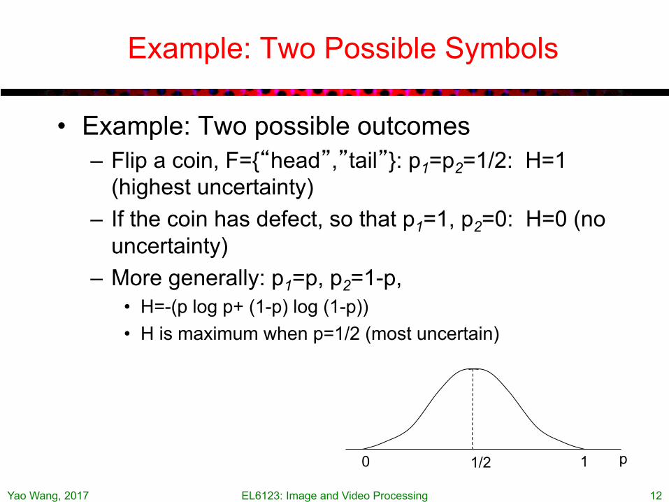
Example: Two Possible Symbols

• Example: Two possible outcomes– Flip a coin, F={“head”,”tail”}: p1=p2=1/2: H=1

(highest uncertainty)– If the coin has defect, so that p1=1, p2=0: H=0 (no

uncertainty)– More generally: p1=p, p2=1-p,

• H=-(p log p+ (1-p) log (1-p))• H is maximum when p=1/2 (most uncertain)

1/20 1 p


Another Example: English Letters

• 26 letters, each has a certain probability of occurrence– Some letters occurs more often: “a”,”s”,”t”, …– Some letters occurs less often: “q”,”z”, …

• Entropy ~= information you obtained after reading an article.

• But we actually don’t get information at the alphabet level, but at the word level!– Some combination of letters occur more often: “it”, “qu”,…


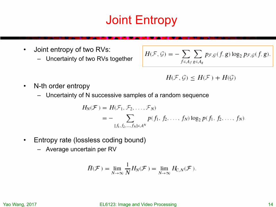
• Joint entropy of two RVs:– Uncertainty of two RVs together

• N-th order entropy– Uncertainty of N successive samples of a random sequence

• Entropy rate (lossless coding bound)– Average uncertain per RV

Joint Entropy


Conditional Entropy

• Conditional entropy between two RVs:– Uncertainty of one RV

given the other RV

• M-th order conditional entropy


Example: 4-symbol source

• Four symbols: “a”,”b”,”c”,”d”• pmf:

• 1st order conditional pmf: qij=Prob(fi|fj)

• 2nd order pmf:

• Go through how to compute H1, H2, Hc,1.

]1154.0,1703.0,2143.0,5000.0[=Tp

0938.01875.0*5.0)"/""(")"(")"(" Ex. === abqapabp


Mutual Information

• Mutual information between two RVs :– Information provided by G about F

• N-th order mutual information (lossy coding bound)


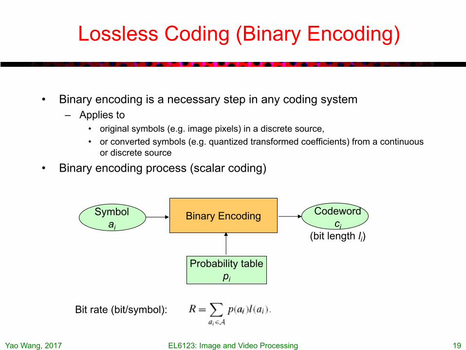
Lossless Coding (Binary Encoding)

• Binary encoding is a necessary step in any coding system– Applies to

• original symbols (e.g. image pixels) in a discrete source, • or converted symbols (e.g. quantized transformed coefficients) from a continuous

or discrete source

• Binary encoding process (scalar coding)

Binary Encoding Codewordci

(bit length li)

Symbolai

Probability tablepi

Bit rate (bit/symbol):


Bound for Lossless Coding

• Scalar coding:– Assign one codeword to one symbol at a time– Problem: could differ from the entropy by up to 1 bit/symbol

• Vector coding:– Assign one codeword for each group of N symbols– Larger N -> Lower Rate, but higher complexity

• Conditional coding (context-based coding)– The codeword for the current symbol depends on the pattern (context) formed

by the previous M symbols

!!

RN(F):bits!for!N!symbolsRN(F)= RN(F)/N : !bits!per!symbol


Binary Encoding: Requirement

• A good code should be:– Uniquely decodable– Instantaneously decodable – prefix code (aka prefix-free code)


Huffman Coding

• Idea: more frequent symbols -> shorter codewords• Algorithm:

• Huffman coding generate prefix code J• Can be applied to one symbol at a time (scalar coding), or a group of symbols (vector coding), or one symbol conditioned on previous symbols (conditional coding)


Huffman Coding Example:Scalar Coding

Huffman Coding Example:Vector Coding



Huffman Coding Example:Conditional Coding

6922.1,8829.1,5016.17500.1,9375.1,5625.1

1,"","","","",

1,"","","","",

=====

=====

CdCcCbCaC

CdCcCbCaC

HHHHHRRRRR


Arithmetic Coding (Not Required)

• Basic idea: – Represent a sequence of symbols by an interval with length d equal to its

probability p– The interval is specified by its lower boundary (l), upper boundary (u) and

length d (=probability)– The codeword for the sequence is the common bits in binary representations of

l and u– Theoretically, no. bits (B) = ceiling( -log2 d)=ceiling (- log2 p)– A more likely sequence=a longer interval=fewer bits

• The interval is calculated sequentially starting from the first symbol– The initial interval is determined by the first symbol– The next interval is a subinterval of the previous one, determined by the next

symbol


Huffman vs. Arithmetic Coding

• Huffman coding (assuming vector coding of N symbols together)– Convert a fixed number of N symbols into a variable length codeword– Efficiency:

– To approach entropy rate, must code a large number of symbols together– Used in all earlier image and video coding standards

• Arithmetic coding (not required)– Convert a variable number of symbols into a variable length codeword– Efficiency:

– Can approach the entropy rate by processing one symbol at a time– Easy to adapt to changes in source statistics– Integer implementation is available, but still more complex than Huffman coding

with a small N– Used as advanced options in earlier image and video coding standards (JPEG,

H264 and before)– Standard options in newer standards (JPEG2000, HEVC)

N is sequence length


Summary on Binary Coding

• Coding system: – original data -> model parameters -> quantization-> binary encoding– Waveform-based vs. content-dependent coding

• Characterization of information content by entropy– Entropy, Joint entropy, conditional entropy – Mutual information

• Lossless coding– Bit rate bounded by entropy rate of the source– Huffman coding:

• Scalar, vector, conditional coding • can achieve the bound only if a large number of symbols are coded together• Huffman coding generates prefix code (instantaneously decodable)

– Arithmetic coding• Can achieve the bound by processing one symbol at a time• More complicated than scalar or short vector Huffman coding

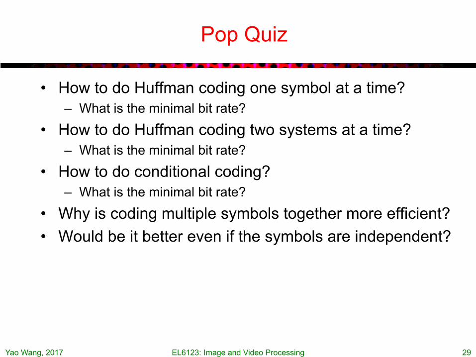
Pop Quiz

• How to do Huffman coding one symbol at a time?– What is the minimal bit rate?

• How to do Huffman coding two systems at a time?– What is the minimal bit rate?

• How to do conditional coding?– What is the minimal bit rate?

• Why is coding multiple symbols together more efficient?• Would be it better even if the symbols are independent?



Lossy Coding

• Original source is discrete– Lossless coding: bit rate >= entropy rate– One can further quantize source samples to reach a lower rate

• Original source is continuous– Lossless coding will require an infinite bit rate!– One must quantize source samples to reach a finite bit rate– Lossy coding rate is bounded by the mutual information

between the original source and the quantized source that satisfy a distortion criterion

• Quantization methods• Scalar quantization: quantize one variable at a time• Vector quantization: quantize one vector (containing multiple

variables) at a time, to exploit the correlation between these variables


Scalar Quantization

• General description• Uniform quantization• MMSE quantizer• Lloyd algorithm


SQ as Line Partition

ll

l

lll

l

BfgfQgbbB

bL

Î=

= -

if ,)( :mappingQuantizer :stion valueReconstruc

),[ :regionsPartition :aluesBoundary v

:levelson Quantizati

1


Function Representation

ll BfgfQ Î= if ,)(


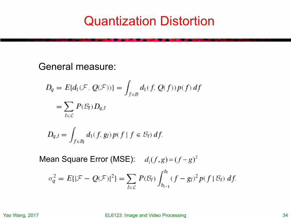
Quantization Distortion

General measure:

Mean Square Error (MSE): 21 )(),( gfgfd -=


Uniform Quantization

Uniform Quantizer for Uniform Source


Uniform source:

Each additional bit provides 6dB gain!

Quantization error e=f-Q(f) is also uniform in (-q/2, q/2), q=B/N=B 2-R

𝜎"#=$% ∫ 𝑓#𝑑𝑓 = %*

$#%/#,%/#

p(f)

f

B

p(e)

eq/2-q/2

Truncated uniform quantization for sources with infinite range


f

Q(f)

t0 =-∞ t1 t2 t3 t4 t5 t6 t7fmin fmax

r0=fmin+q/2

r1

r2

r3

r4

r5

r6

r7=fmax-q/2

overloadregion

overloadregion

t8 =∞

Example

• Suppose the signal has the following distribution. We use a uniform quantizer with three levels, as indicated below. What is the quantization MSE?


pF(f)

f -1 1

1

0 2/3 -2/3 1/3 -1/3


Minimum MSE (MMSE) Quantizer

• Special case: uniform source– MSE optimal quantizer = Uniform quantizer

MSE minimize to, Determine ll gb

:yields 0 0, Setting22

=¶

=¶

l

q

l

q

gbss

(Nearest Neighbor Condition)

(Centroid Condition)

or

Example

• Going back to the previous example. What is the MMSE quantizer(partition levels, reconstruction levels) and corresponding MSE?


pF(f)

f -1 1

1


High Resolution Approximation of MMSE Quantizer

• For a source with arbitrary pdf, when the rate is high so that the pdf within each partition region can be approximated as flat:

1 :sourceGaussian for Bound

VLC) (w/o 71.2 :sourceGaussian i.i.d

1 :source Uniform

2

2

2

=

=

=

e

e

e

(achievable only if coding many many Gaussian variables together)

Pop Quiz

• Suppose the output of a CCD sensor (usually in terms of voltage) is in the range of (0,1) (volt), and you want to represent each pixel using 8 bit.

• What would be the uniform quantizer?– How many levels? – What is the step size?

• Will it be optimal (i.e. minimize MSE)?• How would you go about ”optimal” design?



Vector Quantization

• General description• Nearest neighbor quantizer• MMSE quantizer• Generalized Lloyd algorithm


Vector Quantization: General Description

• Motivation: quantize multiple random variables together, to exploit the correlation between these variables. Treat these RVs as a random vector. E.g. the color of a pixel is a random vector of 3 RVs.

• All possible vectors are distributed in a high dimensional space.• Quantization can be thought of as clustering all possible points to a

finite number of clusters, with all points in the same cluster qunatized into a single centroid of the cluster.

• Applications:– Color quantization: Quantize all colors appearing in an image to L

colors for display on a monitor that can only display L distinct colors at a time – Adaptive palette

– Image quantization: Quantize every NxN block into one of the L typical patterns (obtained through training). More efficient with larger block size, but block size are limited by complexity.


VQ as Space Partition or Clustering

Every point in a region (Bl) is replaced by (quantized to) the point indicated by the circle (gl)

LN

R

LlCBQ

BLR

l

ll

l

l

N

2log1 :rateBit

},...,2,1,{ :Codebook if ,)( :mappingQuantizer :(codeword)r tion vectoReconstruc

:regionsPartition :levelson Quantizati

: vectorOriginal

=

==Î=

Î

gfgfg

f

Clustering view: Each region is a cluster. The codeword for a region is the cluster centroid.


Distortion Measure

Mean quantization distortion:

Square error:

Distortion in each partition region:


Nearest Neighbor (NN) Quantizer(Given the codebook)

Challenge: How to determine the codebook?


Complexity of NN VQ

• Complexity analysis:– Must compare the input vector with all the codewords– Each comparison takes N operations– Need L=2^{NR} comparisons– Total operation = N 2^{NR} – Total storage space = N 2^{NR} – Both computation and storage requirement increases exponentially with N!

• Example: – N=4x4 pixels, R=1 bpp: 16x2^16=2^20=1 Million operation/vector– Apply to video frames, 720x480 pels/frame, 30 fps: 2^20*(720x480/16)*30=6.8

E+11 operations/s !– When applied to image, block size is typically limited to <= 4x4

• Fast algorithms:– Structured codebook so that one can conduct binary tree search– Product VQ: can search subvectors separately


Codebook Design (= Clustering of Training Samples)

• Necessary conditions for minimizing distortion– Nearest neighbor condition: region Bl includes all f that are

closest to gl

– Generalized centroid condition:

– MSE as distortion: centroid= cluster mean


Generalized Lloyd Algorithm

(LBG Algorithm=K-Means)

• Start with initial codewords

• Iterate between finding best partition using NN condition, and updating codewords using centroid condition

Example



Caveats L

Both quantizers satisfy the NN and centroid condition, but the quantizer on the right is better!

NN and centroid conditions are necessary but NOT sufficient for MSE optimality!

Pop Quiz

• Why VQ can be more efficient than SQ in representing a signal? (More efficient means using fewer bits to reach the same distortion)

• What are the two steps in the K-means algorithm for designing the codebook

• Will it always converge?• Will it always converge to the “best” solution?


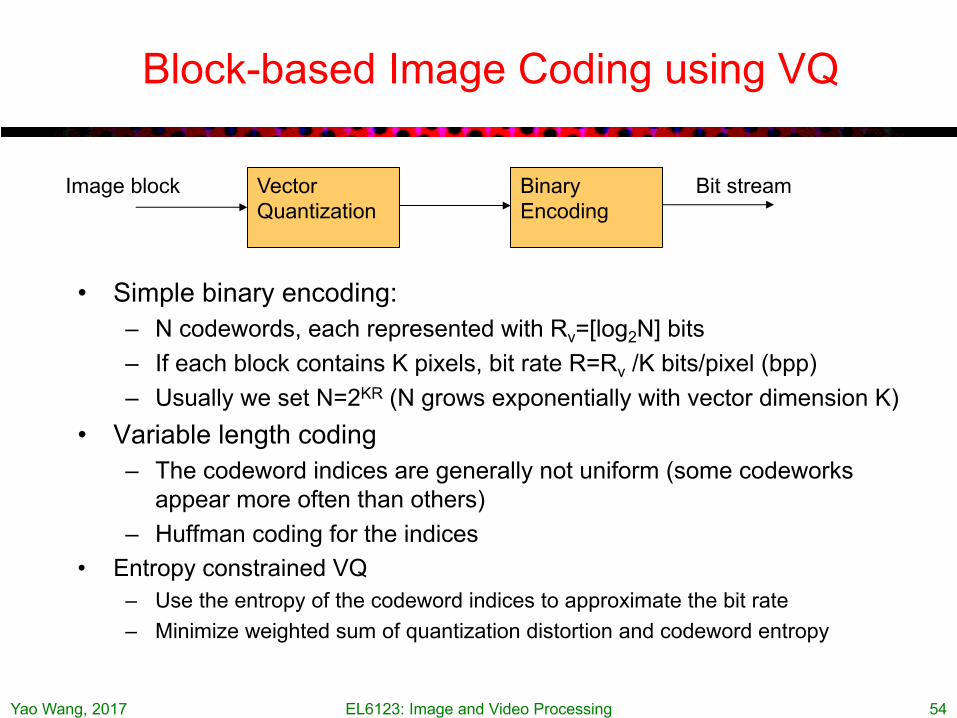
Block-based Image Coding using VQ

• Simple binary encoding: – N codewords, each represented with Rv=[log2N] bits– If each block contains K pixels, bit rate R=Rv /K bits/pixel (bpp)– Usually we set N=2KR (N grows exponentially with vector dimension K)

• Variable length coding – The codeword indices are generally not uniform (some codeworks

appear more often than others)– Huffman coding for the indices

• Entropy constrained VQ– Use the entropy of the codeword indices to approximate the bit rate– Minimize weighted sum of quantization distortion and codeword entropy


Vector Quantization

Image block Binary Encoding

Bit stream


Rate-Distortion Characterizationof Lossy Coding

• Operational rate-distortion function of a quantizer:– Relates rate and distortion: R(D)– A vector quantizer reaches a different point on its R(D) curve by using a

different number of codewords– Can also use distortion-rate function D(R)

• Rate distortion bound for a source– Minimum rate R needed to describe the source with distortion <=D

• RD optimal quantizer:– Minimize D for given R or vice versa

Typical D(R) curve

R

D

(bound) )(RD

quantizer)given (a )(RD


Lossy Coding Bound (Shannon Lossy Coding Theorem, Not required)

IN(F,G): mutual information between F and G, information provided by G about FQD,N: all coding schemes (or mappings q(g|f)) that satisfy distortion criterion dN(f,g)<=D

h(F): differential entropy of source FRG(D): RD bound for Gaussian source with the same variancei.i.d. Gaussian source requires highest bit rate!


RD Bound for Gaussian Source (Not required)

• i.i.d. 1-D Gaussian:

• i.i.d. N-D Gaussian with independent components:

• N-D Gaussian with covariance matrix C:

• Gaussian source with power spectrum (FT of correlation function)


Summary on Quantization

• Scalar quantization:– Uniform quantizer– MMSE quantizer (Nearest neighbor and centroid condition)

• Closed-form solution for some pdf• Lloyd algorithm for numerical solution

• Vector quantization– Nearest neighbor quantizer– MMSE quantizer (Nearest neighbor and centroid condition)– Generalized Lloyd alogorithm– Uniform quantizer

• Can be realized by lattice quantizer (not discussed here)• Rate distortion characterization of lossy coding (not required)

– Bound on lossy coding– Operational RD function of practical quantizers


References

• Reading assignment:– [Wang2002] Wang, et al, Digital video processing and

communications. Sec. 8.1-8.4 (Sec. 8.3.2,8.3.3 optional), 8.5-8.7• Optional reading on arithmetic coding and CABAC

– Witten, Radford, Neal, Cleary, “Arithmetic Coding for Data Compression” Communications of the ACM, vol. 30, no. 6, pp. 520-540, June 1987.

– Marpe, Detlev, Heiko Schwarz, and Thomas Wiegand. "Context-based adaptive binary arithmetic coding in the H. 264/AVC video compression standard." Circuits and Systems for Video Technology, IEEE Transactions on 13.7 (2003): 620-636.

– http://www.hhi.fraunhofer.de/fields-of-competence/image-processing/research-groups/image-video-coding/statistical-modeling-coding/fast-adaptive-binary-arithmetic-coding-m-coder.html

Written Assignment: Binary coding and quantization

• Answer all quizes• Problems from [Wang2002] Prob. 8.1,8.6, 8.11, 8.14• Additional problems in the following slides


Written assignment (2)


Written assignment (3)


Computer assignment (Optional!)

• Do one of the two– Option 1: Write a program to perform vector quantization on a gray scale image

using 4x4 pixels as a vector. You should design your codebook using all the blocks in the image as training data, using the generalized Lloyd algorithm. Then quantize the image using your codebook. You can choose the codebook size, say, L=128 or 256. If your program can work with any specified codebook size L, then you can observe the quality of quantized images with different L.

– Option 2: Write a program to perform color quantization on a color RGB image. Your vector dimension is now 3, containing R,G,B values. The training data are the colors of all the pixels. You should design a color palette (i.e. codebook) of size L, using generalized Lloyd algorithm, and then replace the color of each pixel by one of the color in the palette. You can choose a fixed L or let L be a user-selectable variable. In the later case, observe the quality of quantized images with different L.


Reviews of Random Variables

• Not covered during the lecture. Review at the end of the slide

• What is random variables• A single RV

– Pdf (continuous RV), pmf (discrete RV)– Mean, variance– Special distributions (uniform, Gaussian, Laplacian, etc.)

• Function of a random variable• Two and multiple RV

– Joint probability, marginal probability– Conditional probability– Conditional mean and co-variance



Distribution, Density, and Mass Functions

• The cumulative distribution function (cdf) of a random variable X, is defined by

• If X is a continuous random variable (taking value over a continuous range)– FX(x) is continuous function.– The probability density function (pdf) of X is given by

• If X is a discrete random variable (taking a finite number of possible values)– FX(x) is step function.– The probability mass function (pmf) of X is given by

x.allfor ),.(Pr)( xXxFX £=

).(Pr)( xXxpX ==

)()( xFdxdxf XX =

The percentage of time that X=x.


Special Cases• Binomial (discrete)

• Poisson distribution

• Normal (or Gaussian) N(µ, σ2)

• Uniform over (x1, x2),

• Laplacian L(µ, b)

.,...,1,0,)1(}{ nkppkn

kXP knk =-÷÷ø

öççè

æ== -

)2/()( 22

21)( sµ

sp--= xexf

ïî

ïíì ££

-=otherwise0

1)( 21

12

xxxxxxf

,...1,0,!

}{ === - kkaekXPk

a

bxeb

xf /||

21)( µ--=

Figures are from http://mathworld.wolfram.com


Expected Values

• The expected (or mean) value of a random variable X:

• The variance of a random variable X:

• Mean and variance of common distributions:– Uniform over range (x1, x2): E{x} = (x1+x2)/2, VarX = (x2-x1)2/12– Gaussian N(µ, σ2): Ex = µ, VarX = σ2

– Laplace L(µ, b): Ex = µ, VarX = 2b2

ïî

ïíì

===åòÎ

¥

¥-

discrete is X if)(continuous is X if)(}{

Xx

XX

xXxPdxxxfXEh

( )( )ïî

ïíì

=-

-==åòÎ

¥

¥-

discrete is X if)(

continuous is X if)(}{

X2

22

x X

XXX

xXPx

dxxfxXVar

h

hs


Functions of Random Variable

• Y=g(X)– Following the example of the lifetime of the bulb, let Y

represents the cost of a bulb, which depends on its lifetime X with relation

• Expectation of Y

• Variance of Y

XY =

ïî

ïíì

===åòÎ

¥

¥-

discrete is X if)()(continuous is X if)()(}{

Xx

XY

xXPxgdxxfxgYEh

( )( )ïî

ïíì

=-

-==åòÎ

¥

¥-

discrete is X if)()(

continuous is X if)()(}{

X2

22

x Y

XYY

xXPxg

dxxfxgYVar

h

hs


Two RVs

• We only discuss discrete RVs (i.e. X and Y for both discrete RVs)

• The joint probability mass function (pmf) of X and Y is given by

• The conditional probability mass function of X given Y is

• Important relations

),.(Pr),( yYxXyxpXY ===

)|.(Pr)/(/ yYxXyxp YX ===

)()/(),( / ypyxpyxp YYXXY =

åÎ

===Yy

XYX yYxXxp ),(.Pr)(


Conditional Mean and Covariance

• Conditional mean

• Correlation

• Correlation matrix

• Covariance

• Covariance matrix

å Î====

X| )|(}|{xyX yYxXxPyXEh

å ÎÎ====

YyX,, ),(}{xYX yYxXxyPXYER

( )( ) YXYXYXYX RYXEC hhhh -=--= ,, }{

[ ] úû

ùêë

é=

þýü

îíì

--úû

ùêë

é--

= 2

2

YXY

XYXYX

Y

X

CC

YXYX

Es

shh

hh

C

[ ] { }{ } { } 222

2

2

, XXXY

XY XEYERRXE

YXYX

E hs +=úû

ùêë

é=

þýü

îíì

úû

ùêë

é=R


Multiple RVs

• The definitions for two RVs can be easily extended to multiple (N>2) RVs, X1,X2, …, XN

• The joint probability mass function (pmf) is given by

• Covariance matrix is

[ ]

úúúúú

û

ù

êêêêê

ë

é

=

ïïþ

ïïý

ü

ïïî

ïïí

ì

---

úúúú

û

ù

êêêê

ë

é

-

--

=

221

22221

11221

221122

11

...............

...

......

NNN

N

N

NN

NN CC

CCCC

XXX

X

XX

E

s

ss

hhh

h

hh

C

),...,,.(Pr),...,,( 221121 NNN xXxXxXxxxp ====

binary encoding and quantization - nyu tandon...

Documents