Binary Classification ProblemLearn a Classifier from the Training Set

Given a training dataset

Main goal: Predict the unseen class label for new data

xi 2 A+ , yi = 1 & xi 2 Aà , yi = à 1

S = f (xi;yi)ììxi 2 Rn;yi 2 f à 1;1g;i = 1;. . .;mg

Find a function by learning from data f : Rn ! R

f (x) > 0) x 2 A+ and f (x) < 0) x 2 Aà

The simplest function is linear: f (x) = w0x + b

Binary Classification ProblemLinearly Separable Case

A-

A+

x0w+ b= à 1

wx0w+ b= + 1x0w+ b= 0

Malignant

Benign

Support Vector MachinesMaximizing the Margin between Bounding Planes

A+

A-

x0w+ b= 1

x0w+ b= à 1

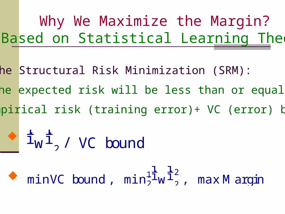
Why We Maximize the Margin?(Based on Statistical Learning Theory)

The Structural Risk Minimization (SRM):

The expected risk will be less than or equal toempirical risk (training error)+ VC (error) bound

íí w

íí

2 / VC bound

minVC bound , min21íí w

íí 2

2 , maxMargin

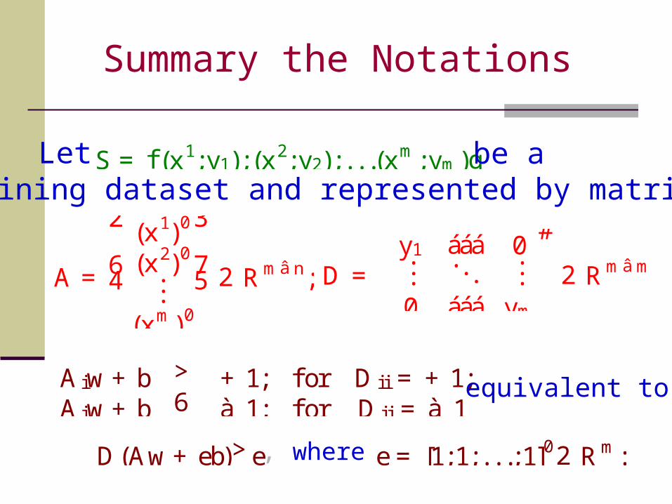
Summary the Notations

Let S = f (x1;y1); (x2;y2); . . .(xm;ym)gbe a training dataset and represented by matrices

A =

(x1)0

(x2)0...

(xm)0

2

64

3

75 2 Rmâ n; D =

y1 ááá 0......

...0 ááá ym

" #

2 Rmâ m

e= [1;1; . . .;1]02 Rm:D(Aw+ eb)>e, where

A iw+ b > + 1; for D ii = + 1;A iw+ b 6 à 1; for D ii = à 1

equivalent to

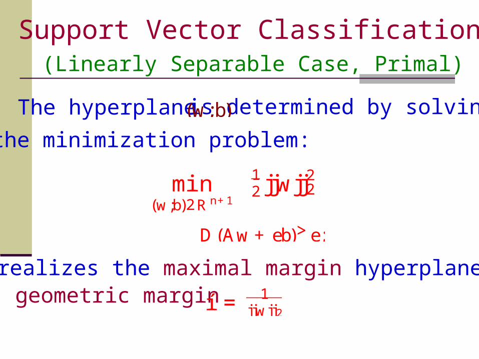
Support Vector Classification(Linearly Separable Case, Primal)

the minimization problem:

The hyperplane is determined by solving (w;b)

min(w;b)2R n+1

21 jjwjj22

D(Aw+ eb)>e;

It realizes the maximal margin hyperplane withgeometric margin í = jjwjj2

1

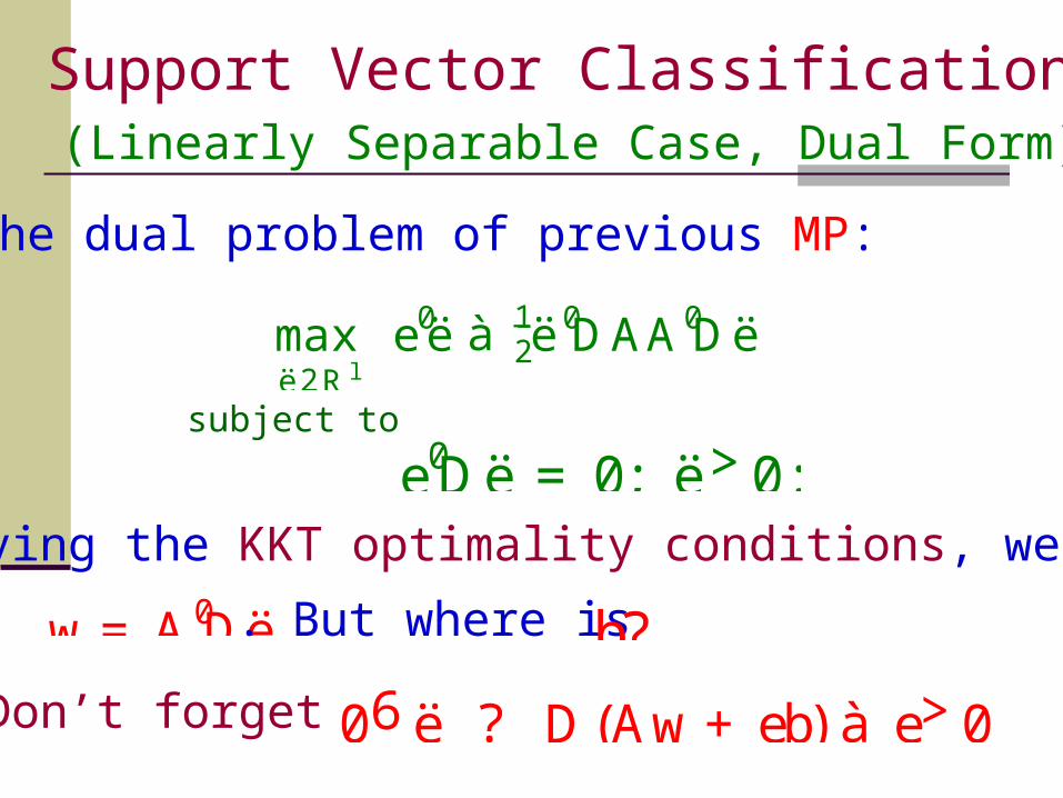
Support Vector Classification(Linearly Separable Case, Dual Form)

The dual problem of previous MP:

maxë2R l

e0ë à 21ë0DAA0Dë

subject to

e0Dë = 0; ë>0:Applying the KKT optimality conditions, we have

w = A0Dë. But where isb?

06ë ? D(Aw+ eb) à e>0Don’t forget

Dual Representation of SVM(Key of Kernel Methods: )

The hypothesis is determined by (ëã;bã)

h(x) = sgn(êx;A0Dëã

ë+ bã)

= sgn(P

i=1

l

yiëãi

êxi;x

ë+ bã)

= sgn(P

ëãi >0

yiëãi

êxi;x

ë+ bã)

w = A0Dëã =P

i=1

`yiëã

i A0i

Remember : A0i = xi

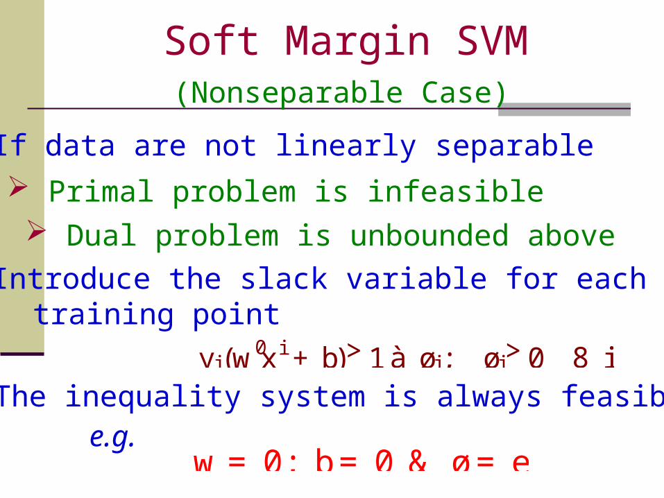
Soft Margin SVM(Nonseparable Case)

If data are not linearly separable Primal problem is infeasible Dual problem is unbounded above

Introduce the slack variable for each training point

yi(w0xi + b)>1à øi; øi>0 8 i The inequality system is always feasible

w = 0; b= 0 & ø= ee.g.

xj

x

x

x

x

x

x

x

x

o

o

o

o

o

o

o

oi

í

í

øj

øi

D(Aw+ eb) >e+ øø>0

whereø: nonnegative slack (error) vector

The term e0ø , 1-norm measure of error vector, is

called the training error.

minw;b;ø

e0ø

s.t. (LP)

Robust Linear ProgrammingPreliminary Approach to SVM

For the linearly separable case, at solution of (LP):

ø= 0

min(w;b;ø)2R n+1+l

21jjwjj22 + 2

Cjjøjj22

D(Aw+ eb) + ø>e

2-Norm Soft Margin:

1-Norm Soft Margin (Conventional SVM):

min(w;b;ø)2R n+1+l

21jjwjj22 + Ce0ø

D(Aw+ eb) + ø>e

ø> 0

Support Vector Machine Formulations(Two Different Measures of Training Error)

Tuning ProcedureHow to determine C?

overfitting

The final value of parameter is one with the maximum testing set correctness !

C

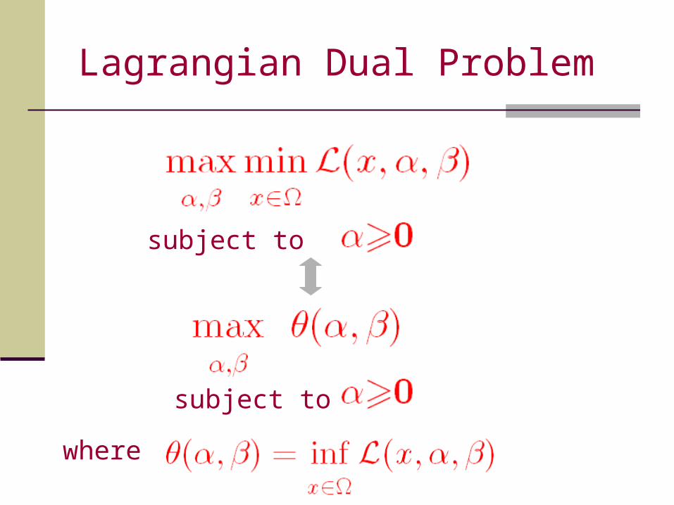
Lagrangian Dual Problem

subject to

subject to

where

1-Norm Soft Margin SVM Dual Formulation

The Lagrangian for 1-norm soft margin:

L (w;b;ø;ë;r) = 21w0w+ Ce0ø+

ë0[eà D(Aw+ eb) à ø]à r0øwhere ë>0 & r>0

The partial derivatives with respect to primalvariables equal zeros

@w@L (w;b;ø;ë) = wà A0Dë = 0

@b@L (w;b;ø;ë) = e0Dë = 0;

@ø@L (w;b;ø;ë) = Ceà ë à r = 0

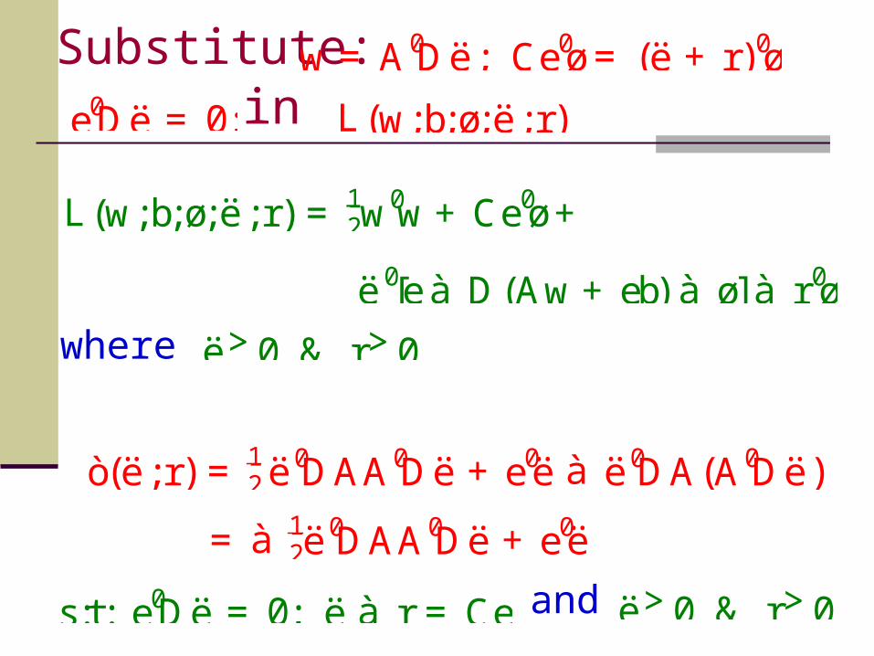
Substitute:

L (w;b;ø;ë;r) = 21w0w+ Ce0ø+

ë0[eà D(Aw+ eb) à ø]à r0ø

where ë>0 & r>0

w = A0Dë; Ce0ø= (ë + r)0ø

in L(w;b;ø;ë;r)e0Dë = 0;

ò(ë;r) = 21ë0DAA0Dë + e0ë à ë0DA(A0Dë)

= à 21ë0DAA0Dë + e0ë

s:t: e0Dë = 0; ë à r = Ce ë>0 & r>0and

Dual Maximization Problemfor 1-Norm Soft Margin

Dual:

0 6 ë 6 Ce

maxë2R l

e0ë à 21ë0DAA0Dë

e0Dë = 0

The corresponding KKT complementarity:

06ë ? D(Aw+ eb) + øà e>0

06ø ? ë à Ce60

Slack Variables for 1-Norm Soft Margin SVM

Non-zero slack can only occur when ëãi = C

The points for which 0< ëãi < C lie at the

bounding planes This will help us to find bã

The contribution of outlier in the decision

rule will be at most C The trade-off between accuracy and

regularization directly controls by C

f (x) =P

ëãi >0

yiëãi

êxi;x

ë+ bã

Two-spiral Dataset(94 White Dots & 94 Red Dots)

Learning in Feature Space(Could Simplify the Classification Task)

Learning in a high dimensional space could degrade

generalization performance This phenomenon is called curse of dimensionality

By using a kernel function, that represents the innerproduct of training example in feature space, we never need to explicitly know the nonlinear map.

Even do not know the dimensionality of feature space There is no free lunch

Deal with a huge and dense kernel matrix

Reduced kernel can avoid this difficulty

X Fþ

þ( ) þ( )

þ( )þ( )

þ( )

þ( )

þ( )þ( )

f (x) =ð P

j=1

?

wjþj(x)ñ

+ b

Linear Machine in Feature Space

Let þ : X ! Fbe a nonlinear map from the

input space to some feature space

The classifier will be in the form (Primal):

Make it in the dual form:

f (x) =ð P

i=1

lë iyi

êþ(xi) áþ(x)

ëñ+ b

K (x;z) =êþ(x) áþ(z)

ë

Kernel: Represent Inner Product in Feature Space

The classifier will become:

f (x) =ð P

i=1

lë iyiK (xi;x)

ñ+ b

Definition: A kernel is a functionK : X â X ! Rsuch thatfor all x;z 2 X

where þ : X ! F

A Simple Example of KernelPolynomial Kernel of Degree 2: K (x;z) =

êx;z

ë2

Let x = x1

x2

ô õ

;z = z1

z2

ô õ2 R2 and the nonlinear map

þ : R27! R3 defined by þ(x) =x2

1

x22

2p

x1x2

2

4

3

5.

Thenêþ(x);þ(z)

ë=

êx;z

ë2= K (x;z).

There are many other nonlinear maps, (x), that

satisfy the relation:ê (x); (z)

ë=

êx;z

ë2= K (x;z)

Power of the Kernel Technique

Consider a nonlinear map þ : Rn7! Rp that consists

of distinct features of all the monomials of degree d.

Then p = n + dà 1d

ð ñ.

For example: n = 11; d = 10; p = 92378

Is it necessary? We only need to know êþ(x);þ(z)

ë!

This can be achieved

K (x;z) =êx;z

ëd

x31x

12x

43x

44 ) â î î î â î â î î î î â î î î î

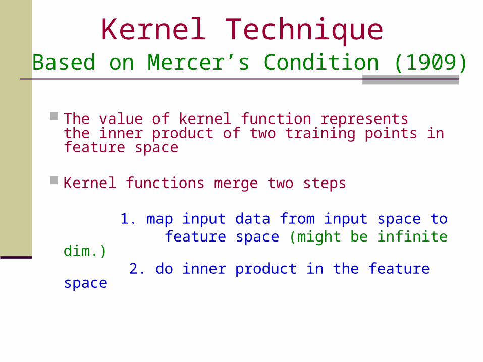
The value of kernel function represents the inner product of two training points in feature space

Kernel functions merge two steps

1. map input data from input space to feature space (might be infinite dim.) 2. do inner product in the feature space

Kernel TechniqueBased on Mercer’s Condition (1909)

More Examples of Kernel

K (A;B) : Rmâ n â Rnâ l 7à! Rmâ l

A 2 Rmâ n;a 2 Rm;ö 2 R; d is an integer:

Polynomial Kernel :(AA0+ öaa0)dï

)(Linear KernelAA0: ö = 0;d = 1

Gaussian (Radial Basis) Kernel:

"à ökA ià A jk22; i; j = 1;. . .;mK (A;A0)ij =

Theij -entry of K (A;A0) represents the “similarity” of data points A i A jand

Nonlinear 1-Norm Soft Margin SVMIn Dual Form

Linear SVM:

0 6 ë 6 Ce

maxë2R l

e0ë à 21ë0DAA0Dë

e0Dë = 0

Nonlinear SVM:maxë2R l

e0ë à 21ë0DK (A;A0)Dë

0 6 ë 6 Ce

e0Dë = 0

1-norm Support Vector MachinesGood for Feature Selection

C > 0 Solve the quadratic program for some :min Ce0ø+ kwk1

D(Aw+ eb) + ø>eø>0;w;b

s. t. ,, denoteswhere D ii = æ1 A+ Aàor membership.

Equivalent to solve a Linear Program as follows: min

ø>0;w;b;s Ce0ø+ e0s

D(Aw+ eb) + ø>e

à s6w6s

SVM as an Unconstrained Minimization Problem

Hence (QP) is equivalent to the nonsmooth SVM:

minw;b2

C k(eà D(Aw+ eb))+k22 + 2

1(kwk22 + b2)

2C køk2

2+ 21(kwk2

2+ b2)

D(Aw+ eb) + ø>eø>0;w;bmin

s. t.(QP)

Change (QP) into an unconstrained MP

Reduce (n+1+m) variables to (n+1) variables

At the solution of (QP):

where (á)+ = maxf á;0gø= (eà D(Aw+ eb))+

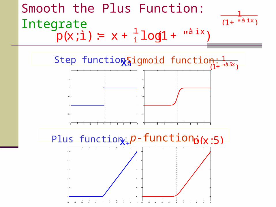
Smooth the Plus Function: Integrate

Step function: xã Sigmoid function:(1+"à 5x)

1

Plus function: x+ p-function: p(x;5)

(1+"à ì x)1

p(x; ì ) := x + ì1 log(1+ "à ì x)

SSVM: Smooth Support Vector Machine

(á)+

Replacing the plus function in the nonsmooth SVM by the smooth p(á; ì ), gives our SSVM:

ìnonsmooth SVM as goes to infinity. The solution of SSVM converges to the solution of

ì = 5(Typically, )

min(w;b) 2 Rn+12

Ckp((eà D(Aw+ eb)); ì )k22 + 2

1(kwk22 + b2)

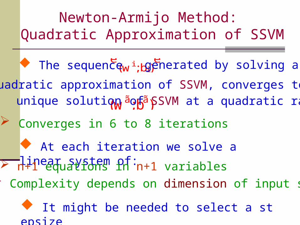
Newton-Armijo Method: Quadratic Approximation of SSVM

At each iteration we solve a linear system of:

n+1 equations in n+1 variables Complexity depends on dimension of input space

Converges in 6 to 8 iterations

(wi;bi)è é

generated by solving a The sequence

(wã;bã)quadratic approximation of SSVM, converges to the

of SSVM at a quadratic rate.unique solution

It might be needed to select a stepsize

Newton-Armijo Algorithm

Start with any (w0;b0) 2 Rn+1. Having(wi;bi);

stop if r Ðì (wi;bi) = 0; else : (i) Newton Direction :

r 2Ðì (wi;bi)di = à r Ðì (wi;bi)0

(ii) Armijo Stepsize :

(wi+1;bi+1) = (wi;bi) + õidi

õi 2 f1;21;4

1; :::g

globally and globally and quadraticallquadratically converge ty converge to unique solo unique solution in a finiution in a finite number of te number of stepsstepssuch that Armijo’s rule is satisfied

Ðì (w;b) = 2Ckp((eà D(Aw+ eb)); ì )k2

2+ 21(kwk2

2+ b2)

Nonlinear Smooth SVM K (x0;A0)Dë + b= 0

K (A;A0) ReplaceAA0by a nonlinear kernel :

2Ckp(eà D(K (A;A0)Dë + eb; ì )k2

2+ 21(këk2

2 + b2)ë;bmin

Use Newton-Armijo algorithm to solve the problem

Each iteration solves m+1 linear equations in m+1 variables

Nonlinear classifier depends on the data points with nonzero coefficients :K (x0;A0)Dë + b=

P

ë j>0ë jyjK (A j ;x) + b= 0

Nonlinear Classifier:

Conclusion

SSVM: A new formulation of support vector machine as a smooth unconstrained minimization problem

No optimization (LP, QP) package is needed

Can be solved by a fast Newton-Armijo algorithm

An overview of SVMs for classification

There are many important issues did not address this lecture such as:

How to solve conventional SVM?

How to deal with massive datasets?

How to select parameters: C & ö

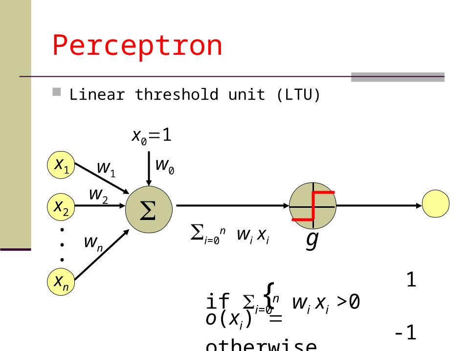
Perceptron

Linear threshold unit (LTU)

x1

x2

xn

.

..

w1

w2

wn

w0

x01

i=0n wi xi

1 if i=0n wi xi >0

o(xi) -1 otherwise{

g

Possibilities for function g

Step functionSign function Sigmoid (logistic) function

step(x) = 1, if x > threshold 0, if x threshold(in picture above, threshold = 0)

sign(x) = +1, if x > 0

-1, if x 0sigmoid(x) = 1/(1+e-x)

Adding an extra input with activation x0 = 1 and weightwi, 0 = -T (called the bias weight) is equivalent to having a threshold at T. This way we can always assume a 0 threshold.

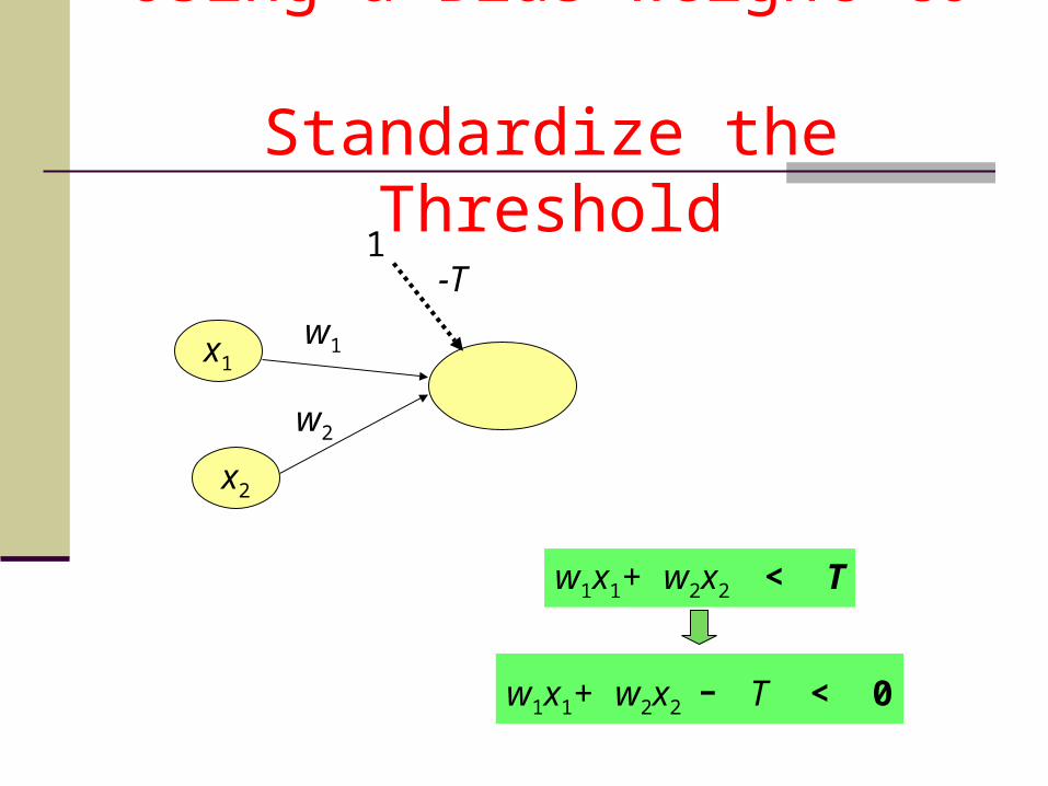
Using a Bias Weight to Standardize the Threshold

1-T

x1

x2

w1

w2

w1x1+ w2x2 < T

w1x1+ w2x2 - T < 0

Perceptron Learning Rule

t = 1

o=1

o=-1

w = [0.2 0.2 0.2]

w = [0.25 –0.1 0.5]x2 = 0.2 x1 – 0.5

t = -1

(x, t)=([-1,-1], 1)o = sgn(0.25+0.1-0.5) =1w = [0.2 –0.2 –0.2]w = [0.2 –0.4 –0.2]

(x, t)=([2,1], 1)o =sgn(0.45-0.6+0.3) =1(x, t)=([1,1], 1)o = sgn(0.250.7+0.1) = 1

x1 x1

x1 x1

x2 x2

x2 x2

-0.5x1+0.3x2+0.45>0 o = 1

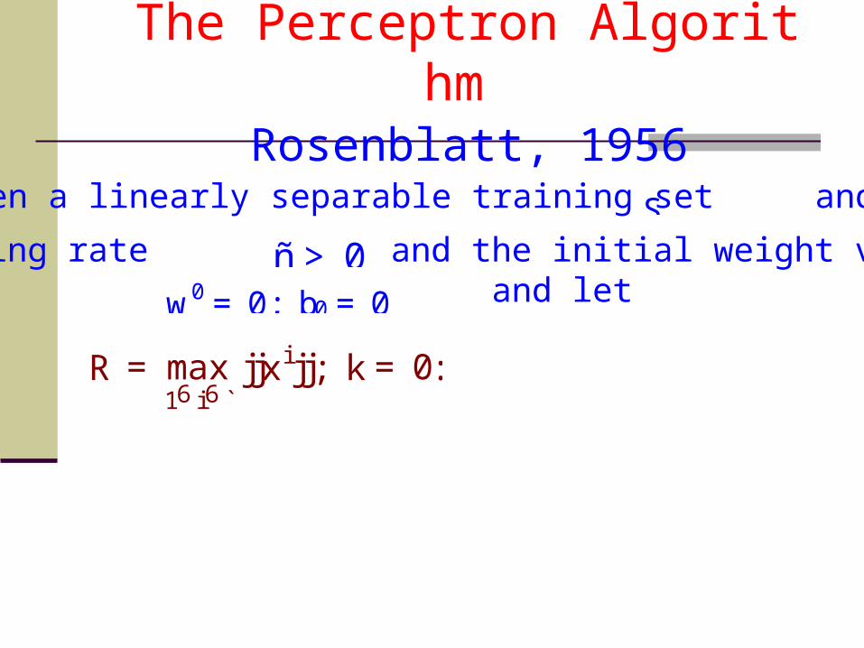
The Perceptron Algorithm Rosenblatt, 1956

Given a linearly separable training set andSñ > 0learning rate and the initial weight vector,

bias: and letw0 = 0; b0 = 0

R = max16 i6 `

jjxijj; k = 0:

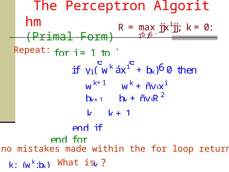
The Perceptron Algorithm (Primal Form)

Repeat: for i = 1 to `

if yi(êwk áxi

ë+ bk)60 then

wk+1 wk + ñyixi

bk+1 bk + ñyiR2

k k + 1end if

until no mistakes made within the for loop return:end for

k; (wk;bk) . What is k ?

R = max16 i6 `

jjxijj; k = 0:

wk+1 wk + ñyixi and bk+1 bk + ñyiR2

yi

àêwk+1 áxi

ë+ bk+1

á> yi

àêwk áxi

ë+ bk

á?

yiàê

wk+1 áxië

+ bk+1á

= yiàê

wk áxië

+ bká

+ ñàê

xi áxië

+ R2á

= yiàê

(wk + ñyixi) áxië

+ bk + ñyiR2á

= yiàê

wk áxië

+ bká

+ yiàñyi

êxi áxi

ë+ R2

á

The Perceptron Algorithm ( STOP in Finite Steps )

Theorem (Novikoff)

SLet be a non-trivial training set, and letR = max16i6`

jjxijj2:

Suppose that there exists a vector wopt 2 Rn; jjwoptjj = 1

and yi(êwopt áxi

ë+ bopt)>í ;8 16 i6 .̀ Then the number

of mistakes made by the on-line perceptron algorithmSon is at most ( í

2R)2:

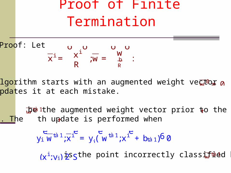
Proof of Finite Termination

Proof: Let

xi = xi

R

ô õ;w =

w

Rb

ô õ:

The algorithm starts with an augmented weight vector and updates it at each mistake.

w0 = 0

Let be the augmented weight vector prior to the th mistake. The th update is performed when

wtà 1

tt

yiêwtà 1;xi

ë= yi(

êwtà 1;xi

ë+ btà 1)60

where is the point incorrectly classified by . (xi;yi) 2 S wtà 1

Update Rule of Perceotron wt wtà 1 + ñyixi ;bt bt + ñyiR2

wt =wt

Rbt

ô õ=

wtà 1

Rbtà 1

ô õ+ ñyi

xi

R

ô õ= wtà 1 + ñyixi:

êwt;wopt

ë=

êwtà 1;wopt

ë+ ñyi

êxi;wopt

ë

>êwtà 1;wopt

ë+ ñí >

êwtà 2;wopt

ë+ 2ñí . . . > tñí

(NOTE : yi(êwopt áxi

ë+ bopt)>í ;8 16 i6 )̀

Similarly,jjwtjj22 = jjwtà 1jj22 + 2ñyi

êwtà 1;xi

ë+ ñ2jjxijj22

6 jjwtà 1jj22 + ñ2jjxijj22 = jjwtà 1jj22 + ñ2(jjxijj22 + R2)

6 jjwtà 1jj22 + 2ñ2R2 6 ááá6 2tñ2R2

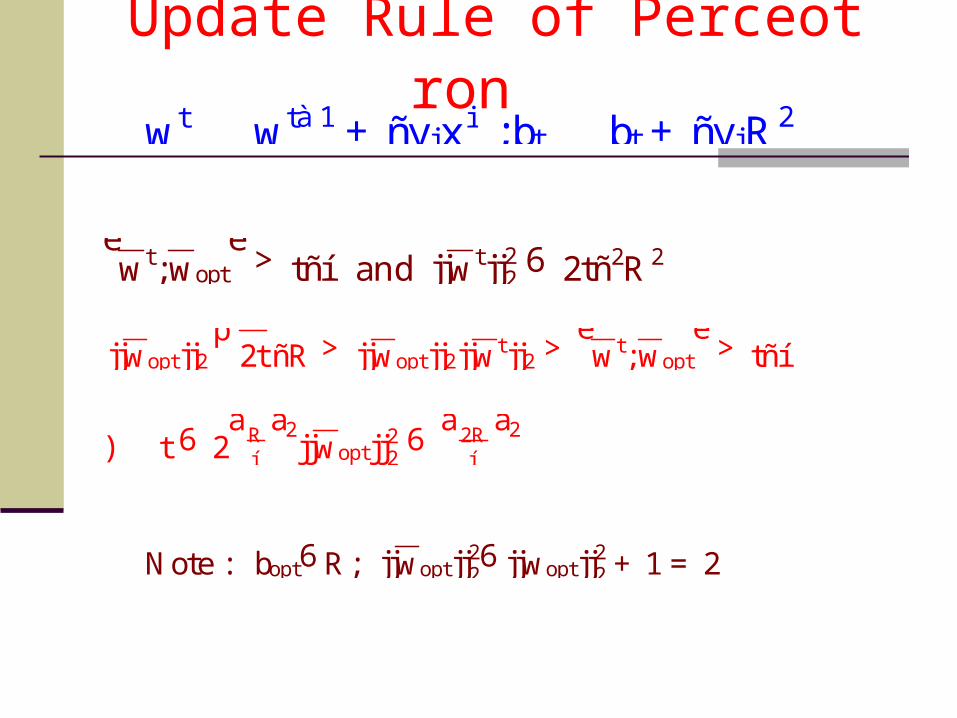
Update Rule of Perceotron wt wtà 1 + ñyixi ;bt bt + ñyiR2

êwt;wopt

ë> tñí and jjwtjj22 6 2tñ2R2

jjwoptjj2 2tp

ñR > jjwoptjj2jjwtjj2 >êwt;wopt

ë> tñí

) t 6 2à

íR

á2jjwoptjj22 6

àí

2Rá2

Note : bopt6R; jjwoptjj226 jjwoptjj22 + 1= 2

The Perceptron Algorithm (Dual Form)

Given a linearly separable training set andS

ë = 0; ë 2 R l ;b= 0;R = max16i6 l jjxijj

w =P

i=1l ë iyixi

Repeat: for i = 1 to l

if yi(P

j=1

l

ë jyjêxj áxi

ë+ b)60 then

ë i ë i + 1; b b+ yiR2

end if

until no mistakes made within the for loop return:

end for

(ë;b)

What We Got in the Dual Form Perceptron Algorithm?

The number of updates equals:P

i=1

l

ë i = jjëjj1 6 ( í2R)2

ë i > 0implies that the training point(xi;yi)has been

misclassified in the training process at least once.

ë i = 0implies that removing the training point(xi;yi)will not affect the final results

The training data only appear in the algorithm through the entries of the Gram matrix, which is defined below:G 2 R lâ l

Gi j =êxi;xj

ë