big islands in dispersing billiard-like...

Physica D 130 (1999) 187–210

Big islands in dispersing billiard-like potentials

Vered Rom-Kedar1,a,∗, Dmitry Turaevb

a The Department of Applied Mathematics and Computer Science, The Weizmann Institute of Science, P.O. Box 26, Rehovot 76100, Israelb Weierstrass Institute for Applied Analysis and Stochastics, Mohrenstr. 39, 10117 Berlin, Germany

Received 6 April 1998; received in revised form 22 January 1999; accepted 28 January 1999Communicated by C.K.R.T. Jones

Abstract

We derive a rigorous estimate of the size of islands (in both phase space and parameter space) appearing in smoothHamiltonian approximations of scattering billiards. The derivation includes the construction of a local return map nearsingular periodic orbits for an arbitrary scattering billiard and for the general smooth billiard potentials. Thus,universalityclasses for the local behavior are found. Moreover, for all scattering geometries and for many types of natural potentials whichlimit to the billiard flow as a parameterε → 0, islands ofpolynomialsize inε appear. This suggests that the loss of ergodicityvia the introduction of the physically relevant effect of smoothening of the potential in modeling, for example, scatteringmolecules, may be of physically noticeable effect. ©1999 Elsevier Science B.V. All rights reserved.

MSC:58F15; 82C05; 34C37; 58F05; 58F13; 58F14

Keywords:Singular Hamiltonian systems; Elliptic islands; Ergodicity; Mixed dynamics

1. Introduction

When an integrable Hamiltonian system is perturbed, non-integrable motion appears [1]. What happens when ahighly chaotic Hamiltonian system is perturbed? In particular, consider an ergodic mixing flow – can a perturbationruin these properties? Clearly, for uniformly hyperbolic systems the answer is negative, e.g., for geodesic flows onthe surfaces of negative curvature [2]. The other basic example for hyperbolic behavior in the Hamiltonian settingis the class of scattering billiards [3]; Billiard motion corresponds to a point particle traveling with a constantspeed in a region, undergoing elastic collisions at the region’s boundary. When the boundary is concave, causingneighboring trajectories to diverge upon reflection, the billiard is called scattering. Due to the divergence instabilitythe scattering billiards are ergodic and mixing systems [3–5]. Thus, these have been suggested [3] as a first step

∗ Corresponding author. Tel.: +1-212-998-3251; fax: +1-212-995-4121; e-mail: [email protected] Present address; Courant Institution of Mathematical Science, 251 Mercer Street, New York University, New York, NY 10012-1185, USA.

0167-2789/99/$ – see front matter ©1999 Elsevier Science B.V. All rights reserved.PII: S0167-2789(99)00021-4

188 V. Rom-Kedar, D. Turaev / Physica D 130 (1999) 187–210

models for substantiating the basic assumption of statistical mechanics – the ergodic hypothesis of Boltzmann (seeespecially the discussion and references in [4,6]).

The scattering billiard corresponds to a non-smooth dynamical system which may formally be thought of asa Hamiltonian motion in a singular potential. However, classical molecules move in smooth (though very steep)potentials. Therefore, it is natural to consider the effect of smoothening of the potential on scattering billiards, and inparticular its effect on the ergodic properties. In [7] we proved that smooth scattering billiard-like potentials may giverise to islands, ruining ergodicity (see also [8] for related results concerning the ‘finite range potentials’ problem).Thus, we demonstrated that proving Boltzmann hypothesis for the hard sphere model is a priori insufficient forproving the achievement of thermodynamical equilibrium for a gas.

Islands appearing in highly chaotic regimes were observed in numerous numerical simulations [9,10]. Whilemany of these simulations were carried for the standard map, only recently it has been shown that for largeK it hasa dense set of parameter values for which elliptic islands exist [11]. It is tempting to assume that the numericallyobserved chaotic sea is a nonuniformly hyperbolic set of positive measure; however, no results in this direction haveappeared to the best of our knowledge.

What is clearly known and has, thus, attracted much attention [9,12–16] is that the appearance of islands in large‘chaotic sea’ is of vast significance; First, it implies that the tail of the correlation function has finite range oscillationsfor initial conditions falling in the island. Moreover, around the islands there may be a ‘stickiness’ region, whichinfluences the temporal correlation function of initial conditions from the ‘chaotic sea’. It is suspected that thisstickiness may cause power-law instead of exponential decay of correlations even when the initial conditions lie inthe chaotic sea.

Islands may be useful; When living in a chaotic sea, the islands correspond to stable dynamics in a highly noisyenvironment. This observation may be used in the context of control of chaos (see focus issue in [16]), where itis desirable to switch quickly from highly ordered to highly chaotic behavior. Our construction enables to locateislands in both phase space and parameter space of the smooth billiard-like flow, allowing for a control of suchswitching.

In all applications the size of the islands and their periodicity matters; these define the space and time scaleson which the transition from chaotic to periodic motion is observable. For example, consider the time correlationfunction

C(T ; x(0)) = limτ→∞

1

2τ

∫ τ

−τ

f (x(t))f (x(t + T )) dt. (1)

This function will essentially beN -periodic forx(0) ∈ IN whereIN denotes an island of periodN . Thus, clearly,the difference between the chaotic sea and island behavior will not be seen before time of orderN – demonstratingthe crucial dependence on the periodicity of the islands. Averaging Eq. (1) overx(0) gives the correlation functionfor a general ensemble of initial conditions – clearly the contribution of the time correlation function associatedwith the island is proportional to its area.

Here, we consider a two degrees of freedom Hamiltonian flow associated with

H = p2x

2+ p2

y

2+ V (x, y; γ, ε), (2)

where, asε → 0, the billiard-like potentialV (x, y; γ, ε) vanishes in the interior of the scattering billiard domainDγ and is of finite height on its boundary (see the next section for exact conditions onV ). The parameterε controlsthe steepness of the potential whereasγ controls the billiard geometry. We assume that atγ = 0 the billiard hasa simple singular periodic orbit– namely, a periodic orbit which is tangent to the billiard boundary at exactly onereflection point. In [7] we proved that in such a setting a linearly stable periodic orbit appears in Eq. (2) forε > 0.

V. Rom-Kedar, D. Turaev / Physica D 130 (1999) 187–210 189

Here, we find thatfor typical potentialsV there exist elliptic islands around these periodic orbits and that their sizedepends onε as a power-law – see Theorem 1 and the following discussion.

A natural question that arises here is how prevalent are billiards with simple singular periodic orbits? We arguedin [7] that a most natural conjecture would be that the singular periodic orbits may be obtained by an arbitrarilysmall deformation of the boundary of any dispersing billiard. We also supported this conjecture by some simplenumerical simulations. Our results, thus, mean that elliptic islands may appear at a smoothening of any dispersingbilliard potential, no matter what the specific geometry of the billiard is. Due to presumed exponential decay ofcorrelation in the dispersing billiards [17], one may expect that the typical period of the elliptic islands for thesmoothened billiard-like potential is of order

∼ λ−1 ln ε

whereλ is the Lyapunov exponent of the (non-smoothened) billiard. Thus, even for extremely steep potentials (verysmallε) the period of elliptic islands seems to be not so large. In other words,the differences between the statisticalbehavior of an idealized (billiard) model and its more realistic smooth approximations may become visible on areasonable time scale.

The proof of Theorem 1 includes the construction of the local return map near the periodic singular orbit, see Eq.(12). This map divides the smooth dispersing billiard-like potentials into universality classes, supplying for eachclass a computational tool for estimating the size and location of elliptic islands (see Section 5).

The paper is ordered as follows; in Section 2 we formulate the main results of our paper, in Section 3 we constructthe local return map near a singular periodic orbit (the proofs are in Appendices A and B), in Section 4 we computethe Birkhoff normal form for the local return map and prove that the first Birkhoff coefficient is not identically zero.In Section 5 we discuss the geometrical interpretation of the universality classes which emerge from the local returnmap and give more details regarding the visibility and typical period of the islands we have found.

2. Main result

Consider a plane scattering (or dispersing) billiard – a billiard in a domainD ⊂ R2 which is a complement toa union of a finite number of strictly convex regions. The boundary ofD consists of a finite number of smooth(Cr+1, r ≥ 2) curvesS1, S2, . . . joined at the corner points. The angles between the boundary arcsSi at the cornerpoints are non-zero and the curvature ofSi is bounded away from zero along the arcs.

The billiard defines a dynamical system (the billiard flowbt ): inertial motion of a pointwise particle insideDand elastic reflections at the boundary – the angle of reflection equals the angle of incidence. We consider a billiardwhich possessesa (simple) singularperiodic orbit.

A basic tool in our analysis is the construction of a regularized billiard to a billiard with a singular periodic orbit.Its construction naturally leads to a new definition of stability or multipliers of the singular orbit. We observe thatthese multipliers play an essential role in determining the dynamics near the singular periodic orbit. Thus, we define(see Fig. 1):

Definition. Consider the billiard flow inD which has a singular periodic orbitL. The domainDL is a regularizationof D with respect toL if L is a regular periodic orbit ofDL, namelyDL differs fromD by a local smooth deformationof D near the tangencies ofL and the support of the deformation is bounded away from any regular reflection pointof L.

Definition. Consider the billiard flow inD which has a singular periodic orbitL. The singular multipliers ofL arethe multipliers ofL in a regularization ofD with respect toL.


Fig. 1. Domain regularization· − · − · − · − · is a regularizing deformation ofD w.r.t. L.

Fig. 2. Domain deformation withγ .

Notice that while a singular billiard has many regularizing billiards, the singular multipliers of a singular periodicorbit are uniquely defined (because they depend only on the position of the regular reflection points and on thecurvature of the boundary there).

2.1. Smooth billiard potentials

Consider a smooth Hamiltonian approximation of the given billiard. Namely, consider a two parameter familyht,ε,γ of Cr Hamiltonian flows associated with

H = p2x

2+ p2

y

2+ V (x, y; γ, ε). (3)

We begin with recalling the formulation and the sufficient conditions introduced in [7] which ensure that theHamiltonian flow of Eq. (3) approximates the billiard flow asε → 0 (for a fixedγ ). Furthermore, below wedescribe the required generic dependence onγ .

The potentialV (x, y; γ, ε) tends to zero inside a regionDγ asε → 0 (along with all derivatives, uniformly inany compact subregion ofDγ ) and it tends to infinity outsideDγ , whereDγ=0 = D.

Thus, varyingγ corresponds to changing the shape of the limiting billiard (see Fig. 2) whereas the parameterε

governs the rate at which the Hamiltonian flow approximates the billiard flow inDγ .To have the proper reflection law in the limit, it is necessary that the gradient of the potential stays normal to the

boundary of the billiard asε → 0. We formalize this requirement as follows:In a neighborhood of(∂D\C) (C is the set of corner points) there exists a pattern functionQ(x, y; γ, ε) whose

level lines coincide with the level lines ofV in a small neighborhood of the boundary arcs without the corners andwhich has (along with all derivatives) a finite limit asε → 0 such that atγ = 0 the boundary of the billiard iscomposed of level lines ofQ(x, y; 0, 0):

Q(x, y; 0, 0)|(x,y)∈Si≡ const. (4)

Here, we further assume that these level lines depend smoothly onγ . Thus, atγ 6= 0 they define a deformedbilliard regionDγ so that the original billiard is now embedded in the one-parameter family of scattering billiards.This is done to unfold the appearance of the singular (tangent) periodic orbit in the original billiard flow. Indeed,


Fig. 3. The form of the barrier function near the boundary.

if the dependence ofDγ on γ is in general position (satisfies Eq. (29)), as for example in Fig. 2, then the tangentperiodic orbit disappears, say, atγ < 0 and there is no other periodic orbit in its small neighborhood, whereas atthe opposite sign ofγ two periodic orbits are born, one passing near the former point of tangency without hittingthe boundary and the other has a regular reflection close to that point (see [7] for more details).

The existence of the pattern function implies that for each boundary arcSi there existsa barrier functionWi(Q, ε)

such that near the boundary (in a small neighborhoodNi of Si without the corners)

V (x, y; ε, γ ) = Wi(Q(x, y; γ, ε), ε). (5)

We assume that∇V does not vanish in a finite neighborhood of the boundary arcs, thus:

∇Q|(x,y)∈Ni6= 0 (6)

and

d

dQWi(Q, ε) 6= 0. (7)

Note that the barrier function does not depend explicitly on(x, y) andγ . It describes the growth of the potentialacross the boundary arcs and we consider it as afore-hand given and unchanged (though we allow for smallCr+1

perturbations of the functionQ which describes the geometry of the billiard). We consider a large class of possiblebarrier functions; however, some restrictions are imposed.

First, the barrier functionWi must, asε → 0, tend to zero at eachQ that lies to the inner side ofSi and it musttend to infinity on the outer side (Fig. 3). Now note that by Eq. (7) the value ofQ may be considered as a functionof W (andε) near the boundary arc. At smallε, a finite change inW corresponds to a small change inQ. Therefore,the following condition makes sense:

Asε → +0, for any finite, strictly positive valuesV1 andV2, the functionQ(W ; ε) tends to zero uniformly onthe intervalV1 ≤ W ≤ V2 along with all(r + 1) derivatives.

Potentials of the above structure (e.g., having the form of Fig. 3 near the boundary) will be calledsmooth billiardpotentials. For example, the following barrier functions give rise to such potentials:

ε

Qα, (1 − Qα)1/ε, e−Q/ε, ε| ln Q|α, ε ln . . . | ln Q|, α > 0. (8)

It is proved in [7] that, asε → 0, the Hamiltonian flows (3) with smooth billiard potentialsr-converge to the billiardflow in Dγ , for any finiter. Namely, these convergeCr smoothly to the billiard flow outside any neighborhood ofsingular orbits andC0 converge near tangent trajectories.


2.2. The scaling assumption, asymptotic normal form and elliptic islands

In this paper we impose an additional restriction on the class of smooth billiard potentials which is satisfied by alltypical examples (e.g., Eq. (8)), as demonstrated in Section 2.3. Assume that the barrier functionsW(Q, ε) satisfythe followingscaling assumptionswith respect to rescaling ofQ = δQ + β to Q:

[S] For someδ = δ(ε, H) > 0, β = β(ε, H) andν(ε, H) such thatδ → 0, β → 0, ν/H → 0 asε → 0, thefunction

Wε(Q) = W(δQ + β, ε) − ν

Hδ3/2(9)

converges asε → 0 to aCr+1 functionW0(Q), either forQ > 0or for all real Q. The convergence isCr+1-uniformon any closed finite interval of values ofQ from the domain of definition. Furthermore, the integral∫ +∞

1W ′

ε(q)dq√

q(10)

converges uniformly, for all sufficiently smallε.In this definitionH is the value of energy, see remarks after Theorem 1.The scaling assumption arises naturally when one requires that the local equations of motion near the tangency

will be independent of the small parameterε and the energyH (see Appendix B, in particular the derivation of Eq.(B.11)). We do not have a clear understanding of a ‘physical sense’ of the scaling parametersδ, β, ν. It is, however,clear that the scaling assumption would not be satisfied with an arbitrary choice of them. Only thoseδ, β, ν forwhich the scaling assumption is satisfied are good for our purposes. In the examples below, this requirement definesδ, β, ν (and the limiting functionW0 as well)uniquely.

The convergence of the integral (10) allows one to consider a function

F(v) = −∫ +∞

0W ′

0(v + x2) dx ≡ −1

2

∫ +∞

v

W ′0(Q)

dQ√Q − v

. (11)

This function arises from integrating the local rescaled equations of motion near the tangency (see Appendix B).It is defined either onR+ or onR (i.e., on the domain of definition ofW0) and it isCr -smooth. Indeed, rewrite

F(v) = −∫ 1

0W ′

0(v + x2) dx − 1

2

∫ +∞

v+1W ′

0(Q)dQ√Q − v

.

The smoothness of both the summands is evident.We take a convention (see Eqs. (6) and (7)) that the pattern functionQ increases across the billiard boundary

when moving inwards, therefore,W ′ is negative soF is a positive function.The following theorem is the main result of the paper:

Theorem 1. Consider a scattering billiard which has a simple singular periodic orbit. Consider a two parameterfamily ofCr, r ≥ 5, smooth Hamiltonian flowsht (ε, γ ) of the form(3) with a smooth billiard potential, approx-imating the billiard flow as(ε, γ ) → 0. Assume that the barrier function near the point of tangency satisfies thescaling assumption [S] for someδ(ε, H) and that the associated functionF is such that the range of values ofF ′(v)

includesR−. Finally, assume thatQ dependence onγ is in general position(i.e., Eq. (29)holds).Then, for smallε, in the (γ, ε) plane there exists a wedgeC−δ(ε, H) < γ < C+δ(ε, H) (with some constant

C±) such that for the parameter values in this wedge, on the energy levelH there exist elliptic islands of widthproportional toδ(ε, H).


Proof. The proof occupies Sections 3 and 4. Roughly speaking, we first show (Proposition 1) that the dynamicsof the Hamiltonian flow in an O(δ)-neighborhood of the tangent periodic trajectory is described, asε → 0, by thetwo-dimensional map

u = v, v = ξ

(v + a√

κF(v)

)− (ξ − 2)0 − u. (12)

It is the limit of the two-dimensional return map of the Hamiltonian flow to a local cross-section near the tangenttrajectory, written in some rescaled coordinates.κ is the billiard’s curvature at the tangency and the quantitiesξ

anda (|ξ | > 2, a > 0) are defined by the billiard flow atε = 0, γ = 0; In fact,ξ is just the sum of the singularmultipliers ofL; 0 is the rescaled parameterγ .

We call Eq. (12)the asymptotic normal formof the local Poincaré map near the tangent trajectory. In Proposition(31), we show that the map (12) has an elliptic island of finite size (in the rescaled toδ variablesu andv) for a finiterange of values of0. Returning to the original, non-scaled variables gives theδ-size island which appears in thewedge as stated. �

Few remarks are now in order; first, the theorem implies that given a billiard with a simple singular periodic orbitthere exist one parameter family of Hamiltonian flowsht (ε, γ (ε)) which r-converge to the billiard flow and forwhich elliptic islands of sizeδ(ε, H) exist for allε < ε0.

Second, the size of the island depends, of course, on the choice of the coordinates – we choose the most naturalcoordinates so the theorem applies directly to the islands size as observed in the phase space coordinates (3). To bespecific, given the singular periodic orbitL, we choose the origin as the point of tangency, and thex-axis parallel toL at that point. A local Poincaré map in a neighborhood ofL is defined by takingx = const, and the coordinates onthe cross-section are the variablesy andy′ = py/px (herepx ≈ √

H , hence, when largeH values are consideredthis additional factor arises).

Thirdly, the billiard flow is clearly independent ofH , hence, using assumption [S] it is possible to obtain localreturn map which is independent ofH . It follows that for the Hamiltonian flow islands appear for allH values (andtheir size depends onH via δ(ε, H) and

√H as explained above). For greater genericity, we also allow the chosen

value ofH to depend onε.Finally, the scaling assumption [S] is satisfied by all potentials listed in Eq. (8). Moreover, given a barrier function

W , in many cases, the scaling constantδ and the functionF involved in the above estimate of the size of ellipticislands are fairly easy to compute. Before embarking into the details of the proof, we demonstrate the above statementfor typical examples of the list (8).

2.3. Islands size for specific potentials

Consider the barrier function

W(Q, ε) = ε

Qα.

It satisfies assumption [S] provided

δ(ε, H) =( ε

H

)1/(α+3/2)

, ν = 0, β = 0, (13)

for which

W0(Q) = 1

Qα.


Integration of Eq. (11) gives in this case

F(v) =√

π

2

0(α + 1/2)

0(α)

1

vα+1/2.

The functionF satisfies the condition of the theorem so for such potentials the size of elliptic islands is given byδ of Eq. (13), namely it is polynomial inε/H . Note that the size of islands is larger (asymptotically) for largerα

(though the limitα → ∞ cannot be taken in Eq. (13)).Choosing

W(Q, ε) = exp(−Q/ε)

will satisfy the scaling assumption, provided

δ = ε, ν = 0, β = −ε ln(δ3/2H), (14)

for which

W0(Q) = exp(−Q)

and

F(v) =√

π

2e−v.

Thus, in this case the elliptic islands are of sizeε, independent asymptotically of the value ofH (in the (y, y′)coordinates).

An example which has been used by many authors [18,19] is:

W(Q, ε) = (1 − Qα)1/ε.

It is obviously equivalent to

W(Q, ε) = exp(−Qα/ε)

which is analogous to the previous example; ifε3/2αH → 0, one may assume

δ = ε1/α

α(− ln(ε3/2αH))(1−α)/α, ν = 0, β =

(−ε ln(δ3/2H)

)1/α

. (15)

Here again

W0(Q) = exp(−Q)

and

F(v) =√

π

2e−v.

Thus, the islands size is again polynomial inε. The critical exponent ofH ∝ ε−3/(2α) arises from the analysis –if H grows faster – different asymptotics applies. Also, notice the different behavior forα > 1 versusα < 1, againwe see that steeper decay of the potential gives rise to larger islands.


Fig. 4. Auxiliary regular local map near tangency.· − · − · − · − · is the regularization ofD w.r.t. L and . . . is a trajectory of the auxiliaryHamiltonian flow.

Finally, for

W(Q, ε) = ε| ln Q|α

take

δ =(αε

H

)2/3(

2

3

∣∣∣logαε

H

∣∣∣)2(α−1)/3

, ν = ε| ln δ|α, β = 0, (16)

for which

W0(Q) = − ln Q

and

F(v) = π

2√

v.

3. The Poincaré map near a tangent periodic orbit

Here, we formulate and prove Proposition 1 describing the local return map near a simple singular periodic orbit.Consider the two parameter family of Hamiltonian systems (3) with smooth billiard potentials obeying the scalingassumption [S] (by whichδ, β, W (Q) are determined), whichr-converge to the embedding family of the billiardflow with the simple singular periodic orbitL as above.

Choose the coordinates(x, y) such that the origin is at the point of tangency and thex-axis is tangent to theboundary – i.e., it is parallel to the tangent piece of the singular trajectoryL. On a fixed energy levelH take a smalltwo-dimensional cross section6 = {x = −c} to this piece ofL, wherec is some fixed small positive number (seeFig. 4). For greater genericity, we assume thatc may depend onε andγ and it tends to some small positive valueasε, γ → 0.

The variablesy andy′ ≡ py/px serve as the coordinates on6: given fixedy′, the value ofpx is found from theenergy constrain because∂H/∂px ≡ px(1 + y′2) does not vanish on6 due to the choice of the coordinate frame.

Proposition 1. There is a region on the cross-section6 on the energy levelH where the local return mapBε ofthe smooth Hamiltonian flow may be reduced, by an affine transformation(y, y′) 7→ (u, v) which has a finite limit(with non-zero Jacobian) asε → 0, to the form:

u = v + · · ·v = ξ

(v + a√

κδF

(v + · · ·

δ

))− (ξ − 2)vγ − u + · · · (17)


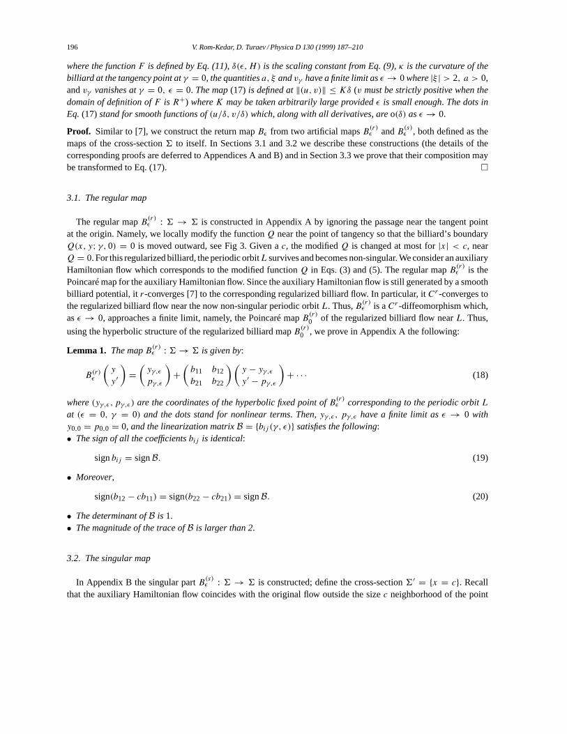
where the functionF is defined by Eq. (11), δ(ε, H) is the scaling constant from Eq. (9), κ is the curvature of thebilliard at the tangency point atγ = 0, the quantitiesa, ξ andvγ have a finite limit asε → 0 where|ξ | > 2, a > 0,andvγ vanishes atγ = 0, ε = 0. The map(17) is defined at‖(u, v)‖ ≤ Kδ (v must be strictly positive when thedomain of definition ofF is R+) whereK may be taken arbitrarily large providedε is small enough. The dots inEq. (17)stand for smooth functions of(u/δ, v/δ) which, along with all derivatives, areo(δ) asε → 0.

Proof. Similar to [7], we construct the return mapBε from two artificial mapsB(r)ε andB

(s)ε , both defined as the

maps of the cross-section6 to itself. In Sections 3.1 and 3.2 we describe these constructions (the details of thecorresponding proofs are deferred to Appendices A and B) and in Section 3.3 we prove that their composition maybe transformed to Eq. (17). �

3.1. The regular map

The regular mapB(r)ε : 6 → 6 is constructed in Appendix A by ignoring the passage near the tangent point

at the origin. Namely, we locally modify the functionQ near the point of tangency so that the billiard’s boundaryQ(x, y; γ, 0) = 0 is moved outward, see Fig 3. Given ac, the modifiedQ is changed at most for|x| < c, nearQ = 0. For this regularized billiard, the periodic orbitL survives and becomes non-singular. We consider an auxiliaryHamiltonian flow which corresponds to the modified functionQ in Eqs. (3) and (5). The regular mapB(r)

ε is thePoincaré map for the auxiliary Hamiltonian flow. Since the auxiliary Hamiltonian flow is still generated by a smoothbilliard potential, itr-converges [7] to the corresponding regularized billiard flow. In particular, itCr -converges tothe regularized billiard flow near the now non-singular periodic orbitL. Thus,B(r)

ε is aCr -diffeomorphism which,asε → 0, approaches a finite limit, namely, the Poincaré mapB

(r)0 of the regularized billiard flow nearL. Thus,

using the hyperbolic structure of the regularized billiard mapB(r)0 , we prove in Appendix A the following:

Lemma 1. The mapB(r)ε : 6 → 6 is given by:

B(r)ε

(y

y′

)=(

yγ,ε

pγ,ε

)+(

b11 b12

b21 b22

)(y − yγ,ε

y′ − pγ,ε

)+ · · · (18)

where(yγ,ε, pγ,ε) are the coordinates of the hyperbolic fixed point ofB(r)ε corresponding to the periodic orbitL

at (ε = 0, γ = 0) and the dots stand for nonlinear terms. Then, yγ,ε, pγ,ε have a finite limit asε → 0 withy0,0 = p0,0 = 0, and the linearization matrixB = {bij (γ, ε)} satisfies the following:• The sign of all the coefficientsbij is identical:

signbij = signB. (19)

• Moreover,

sign(b12 − cb11) = sign(b22 − cb21) = signB. (20)

• The determinant ofB is 1.• The magnitude of the trace ofB is larger than 2.

3.2. The singular map

In Appendix B the singular partB(s)ε : 6 → 6 is constructed; define the cross-section6′ = {x = c}. Recall

that the auxiliary Hamiltonian flow coincides with the original flow outside the sizec neighborhood of the point


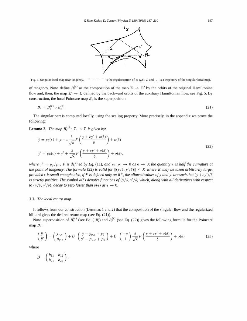
Fig. 5. Singular local map near tangency.· − · − · − · − · is the regularization ofD w.r.t. L and. . . is a trajectory of the singular local map.

of tangency. Now, defineB(s)ε as the composition of the map6 → 6′ by the orbits of the original Hamiltonian

flow and, then, the map6′ → 6 defined by the backward orbits of the auxiliary Hamiltonian flow, see Fig. 5. Byconstruction, the local Poincaré mapBε is the superposition

Bε = B(r)ε ◦ B(s)

ε . (21)

The singular part is computed locally, using the scaling property. More precisely, in the appendix we prove thefollowing:

Lemma 2. The mapB(s)ε : 6 → 6 is given by:

y = y0(ε) + y − cδ√κ

F

(y + cy′ + o(δ)

δ

)+ o(δ)

y′ = p0(ε) + y′ + δ√κ

F

(y + cy′ + o(δ)

δ

)+ o(δ),

(22)

wherey′ = py/px , F is defined by Eq.(11), andy0, p0 → 0 as ε → 0; the quantityκ is half the curvature atthe point of tangency. The formula(22) is valid for ‖(y/δ, y′/δ)‖ ≤ K whereK may be taken arbitrarily large,providedε is small enough; also, if F is defined only onR+, the allowed values ofy andy′ are such that(y +cy′)/δis strictly positive. The symbolo(δ) denotes functions of(y/δ, y′/δ) which, along with all derivatives with respectto (y/δ, y′/δ), decay to zero faster thanδ(ε) asε → 0.

3.3. The local return map

It follows from our construction (Lemmas 1 and 2) that the composition of the singular flow and the regularizedbilliard gives the desired return map (see Eq. (21)).

Now, superposition ofB(r)ε (see Eq. (18)) andB(s)

ε (see Eq. (22)) gives the following formula for the PoincarémapBε :(

y

y′

)=(

yγ,ε

pγ,ε

)+ B

(y − yγ,ε + y0

y′ − pγ,ε + p0

)+ B

(−c

1

)δ√κ

F

(y + cy′ + o(δ)

δ

)+ o(δ) (23)

where

B =(

b11 b12

b21 b22

).


Let us make the affine transformation

v = y + cy′, u = (1, c)B−1(

y − yγ,ε

y′ − pγ,ε

)+ (1, c)

(yγ,ε − y0

pγ,ε − p0

); (24)

recall that detB = 1, hence

B−1 =(

b22 −b12

−b21 b11

).

It is easy to see that this change of coordinates brings the map (23) to the form (17), where

ξ = tr B, (25)

a = (1, c)B(−c, 1)T

ξ(26)

and

vγ = yγ,ε + cpγ,ε − (b11 + b21c − 1)y0 + (b12 + b22c − c)p0

ξ − 2. (27)

Moreover,a > 0 by Eq. (20) and|ξ | > 2 by Eq. (25) (see Lemma 1).Finally, the determinant of the transformation is given by:

J = ∂(u, v)

∂(y, y′)= (1, c)B(−c, 1)T = ξa, (28)

hence it clearly has a finite, non-vanishing limit asε → 0, completing the proof of Proposition 1. �

3.4. Non-degenerate dependence onγ

Here, we establish that under the assumptions of Proposition 1, and if additionally, the dependence of the smoothbilliard potential onγ is in general position, thenvγ of Eq. (17) can be replaced byγ .

Indeed, consider the billiard flow(ε = 0); then from Eq. (27)vγ = 2(yγ,ε=0 + cpγ,ε=0) where the pointMγ = (yγ 0, pγ 0) is the hyperbolic fixed point of the regular map which corresponds to the regularized billiard.Notice that on the cross-section6 : {x = −c} the straight linev = y + cy′ = 0 is tangent to thesingularityline (the curve of initial conditions corresponding to tangent trajectories). Moreover, the pointM0 belongs to thesingularity line by assumption, and by definitionM0 = (0, 0). Thus,v0 = 0. We make the followingnon-degeneracyassumption:

The fixed pointMγ of the regular mapB(r)0 crosses the singularity line with non-zero velocity asγ varies.

Sincev measures the distance from the singularity line, it is equivalent to

∂vγ

∂γ6= 0. (29)

Thusγ may be rescaled so that

vγ ≡ γ. (30)

Notice that the non-degeneracy assumption is formulated in terms of the billiard flow solely; thus, it describeshow the boundary of the billiard depends onγ . It is a condition of general position: if it is not satisfied, it may beeasily achieved by a small smooth perturbation of the functionQ(x, y; γ, 0): the position of the singularity line is


determined only by the local behavior ofQ near the point of tangency whereas the position of the auxiliary fixedpointM is determined only by the local behavior ofQ at the points of regular collision ofL with the boundary.

The non-degeneracy condition is simple and natural when the dependence onγ is localized near the tangent point(e.g., when artificially embedding the singular billiard in a family of billiards as in regularization); in this case theperiodic orbit of the auxiliary billiard does not move asγ varies. This means thaty′

γ = 0. Since the coordinates on6 are defined so that the orbit starting at(y = 0, y′ = 0) is tangent to the boundary, it follows that∂yγ /∂γ 6= 0provided the boundary near the point of tangency moves, asγ varies, with non-zero velocity in the normal direction(e.g., see Fig 4).

4. Islands

To complete the proof of Theorem 1, we now establish that the Poincaré map found in Proposition 1 attainselliptic islands as stated in the Theorem. Let us consider the following rescaling of Eq. (17):

u′ = u

δ, v′ = v

δ, 0 = vγ

δ. (31)

In the new variables the map (17) has the map (12) as a limit asε → 0. Since O(1) intervals in the rescaledvariables correspond to O(δ) intervals in the original variables, it follows that once we show that for a finite rangeof values of0 the map (12) has an elliptic island of a finite size, we are done. The idea is to use KAM-theory inorder to establish the existence of the island around an elliptic periodic point, like in [8,20,21] and in many otherpapers.

Thus, Theorem 1 reduces to the following statement.

Proposition 2. Assume the range of values ofF ′(v) includesR−. Then, for any|ξ | > 2 anda > 0 there exists aninterval of values of0 for which the map(12)has an elliptic fixed point with non-zero first coefficient in the Birkhoffnormal form.

Proof. Fixed points of Eq. (12) are:

uf = vf , 0f (vf ) = vf + aξ√κ(ξ − 2)

F (vf ) (32)

which defines0f (vf ) for all vf in the domain of definition ofF (e.g.,R+). The fixed points are linearly stable ifand only if:

vf ∈ Is ={vf | −

(1 + 2

|ξ |)

<a√κ

F ′(vf ) < −(

1 − 2

|ξ |)}

. (33)

NamelyIs is a union of open intervals of stability invf , which is non-empty if, for example, the range ofF ′(v)

includesR− as required, leading to intervals of the corresponding0f values.On Is, the eigenvalues of the fixed point are e±iω where

cosω = ξ

2

(1 + a√

κF ′(vf )

). (34)

SinceF ′ takes all negative values, there exists at least one interval of linear stability fromIs on which the value ofω runs from 0 toπ .

To prove the lemma we need to show that at least for onevf from the given interval the first coefficient of theBirkhoff normal form at the elliptic fixed point is non-zero (according to Moser theorem this will prove that at thecorresponding value of0 and for all close0, there exists an elliptic island surrounding the fixed point).


The sought Birkhoff coefficient equals to

B(vf ) = − 1

8 sin3ω

(ξa

2√

κF ′′′(vf ) +

(ξa

2√

κF ′′(vf )

)2(1 + 4 cosω)

(1 − cosω)(1 + 2 cosω)

). (35)

Indeed, the linear transformationz = eiω(v − vf ) − (u − uf ) brings the map (12) to the following form near thefixed point:

z = eiωz − ξa√κ

F ′′(vf )eiω

8 sin2ω(z − z∗)2 + i

ξa√κ

F ′′′(vf )eiω

48 sin3ω(z − z∗)3 + · · · (36)

where the dots stand for higher order terms.An arbitrary two-dimensional conservative map near an elliptic fixed point is written as

z = eiωz + eiω(αz2 − 2α∗zz∗ + ηz∗2

)+ eiωβz2z∗ + · · · (37)

where

Reβ = αα∗ − ηη∗ (38)

(which is necessary to have the Jacobian equal to one) and the dots stand for the rest of cubic and higher orderterms. In the case of map (36)

α = η = − ξaF ′′(vf )

8√

κ sin2ω(39)

and

β = −iξaF ′′′(vf )

16√

κ sin3ω. (40)

If ω 6= 2π/3, a simplectic transformation of the form

z′ = z −[

eiωα

e2iω − eiωz2 − 2

eiωα∗

1 − eiωzz∗ + eiωη

e−2iω − eiωz∗2

]+[

(1/2)ηη∗

1 − cos 3ω− (1/2)αα∗

1 − cosω

]z2z∗ + · · · (41)

eliminates all quadratic terms in Eq. (37) and brings it to the form (dropping′)

z = eiωz + ieiωBz2z∗ + · · · (42)

whereB is the first Birkhoff coefficient2 :

B = Imβ + sinω

1 − cosω

[ηη∗ 1 − 2 cosω

1 + 2 cosω− 3αα∗

]. (43)

Plugging Eq. (39) and (40) in Eq. (43) gives Eq. (35).If ω 6= 2π/3, ω 6= π/2, all the other cubic terms in Eq. (42) are non-resonant, hence, they can be eliminated by

the further normalizing transformation. Then, in the simplectic polar coordinatesz = √reiθ the map becomes

r = r + o(r2), θ = θ + ω + Br + o(r). (44)

Whenθ ′r |r=0 ≡ B 6= 0, the KAM-theory is applied to this map at smallr, which gives the existence of the sought

elliptic island.

2 At β = 0 this expression coincides with that found in [20].


Now, note that the quantityB(vf ) given by Eq. (35) cannot be identically zero on the interval of values ofvf

under consideration. Indeed, if for exampleF ′′(vf ) never vanishes, thenB(vf ) tends to infinity when approachingthe bifurcation pointvf = v1

f which corresponds to cosω = 1. One can check that even ifF ′′(v1f ) vanishes but

the zero is of finite order, then stillB(vf ) is not identically zero nearvf = v1f . Indeed, in this case, for some finite

n ≥ 1 andd 6= 0,

F ′(vf ) = F ′(v1f ) + d(vf − v1

f )n + · · · ,

F ′′(vf ) = nd(vf − v1f )n−1 + · · · ,

F ′′′(vf ) = n(n − 1)d(vf − v1f )n−2 + · · · , (45)

then, from Eq. (34)

cosω = 1 + daξ

2√

κ(vf − v1

f )n + · · · (46)

hence, from Eq. (35)

B(vf ) = daξ

16√

κ sin3ωn

(1 + 8

3n

)(vf − v1

f )n−2 + · · · 6≡ 0. (47)

This proves the lemma for the case where the functionF is analytic (as in all our examples). In this case, itfollows thatB may vanish only at isolated points in the interval of stability.

Without the assumption of the analyticity, ifB(vf ) were identically zero on the interval under consideration, wewould have by Eq. (35)

ξa

2√

κF ′′′(vf ) +

(ξa

2√

κF ′′(vf )

)2(1 + 4 cosω)

(1 − cosω)(1 + 2 cosω)= 0 (48)

or, in view of Eq. (34),

d2 cosω

dv2f

+(

d cosω

dvf

)2(1 + 4 cosω)

(1 − cosω)(1 + 2 cosω)= 0. (49)

This equation is easily integrated; on the interval cosω ∈ [−1/2, 1] we get

d cosω

dvf

= c3√

(1 − cosω)5(1 + 2 cosω), (50)

wherec is some constant which cannot be zero because cosω must run all the interval under consideration asvf

varies. At cosω close to 1 we have

d cosω

dvf

∼ (1 − cosω)5/3. (51)

This means thatω never approaches zero at finitevf which contradicts the initial assumption (that the range ofF ′ includes all negative values, see Eq. (34)). �

As an example, consider numerical simulations of the map (12) forW(Q) = ε/Q which confirm the existenceof O(1) islands; the map (12) becomes:

u = v

v = ξv − (ξ − 2)0 − u + ξπ

4

a√κ

1

v3/2(52)


Fig. 6. Rescaled local map near singular periodic orbit. Orbits of Eq. (52) (W(Q) = ε/Q, ξ = 4, π/4a/√

κ = 1) (a)0 = 2.6, (b)0 = 2.8, (c)0 = 3.

Taking ξ = 4, (π/4)(a/√

κ) = 1 makesIs = (1, 30.4 ≈ 1.5518) and thus an interval of stability for0 ∈((5/3)30.4 ≈ 2.586, 3.), Fig. 6 confirms the existence of elliptic island for0 = 2.6, 2.8. In fact it is seen that evenfor 0 = 3. the stability island still exists.

5. Discussion

Our main result, Theorem 1, together with assumption [S], supplies a computational tool for estimating the sizeof elliptic islands for specific potentials. For natural Hamiltonians which appear in physical setting, the estimatedsize of the islands is polynomial inε, whereε is the small parameter which controls the steepness of the potentialnear the core. Moreover, the dependence of the islands size on the energy has also been explicitly computed (seeSections 2.2 and 2.3) and is also typically polynomial.

Furthermore, we introduced the notion of singular multipliers for tangent periodic orbits of billiard. Thesemeasure the impact of the singular periodic orbit. In our setting these multipliers play a central role in the dynamicsas explained next. We believe billiards with singular periodic orbits are dense among scattering billiards, hence thatthe concept of singular multipliers may be useful in other investigations of billiard problems.


While proving the rigorous estimates for the islands size, we have constructed the following local map nearsingular periodic orbits (12):

u = v

v = ξv + aξ√κ

F(v) − u + (ξ − 2)0.(53)

This map defines universality classes – large classes of different billiard geometries and different potentials giverise to exactly the same local map. The Jacobian of the transformation to this map isJ = ξa/δ2 and the unfoldingparameter0 = vγ /δ, see Eqs. (25), (26) and (28). Nowδ andF(·) are the rescaling parameter and rescaling functionwhich depend only on the rate at which the smooth billiard potential approaches a billiard – they are independentof the billiard geometry (see Section 2.3 for examples ofδ, F ). Conversely,κ, ξ, a are parameters which dependonly on the billiard flow (the geometry):κ is the local curvature near the tangent periodic orbit (local parameter).ξ is the sum of the singular multipliers measuring the instability of the singular periodic orbit (global parameter,independent of the local structure near tangency). The parametera measures, roughly, how the regular flow rotatesthe singularity line – the larger thea the closer the image of the singularity line to its normal. The larger theξ thecloser this image is to the unstable eigenvector of the regularized billiard return map, thus for largeξ , the quantitya measures the alignment between this eigenvector and the normal to the singularity line.

Summarizing, the coefficient of the nonlinear term in Eq. (17) is given by(1/√

κ)ξa which shows how thecurvature, the singular multipliers and the global billiard geometry effects (respectively) scale together to create asignificant nonlinear term.

5.1. Are the islands observable?

The disappearance of two hyperbolic periodic orbits via a simple singular periodic orbit is a codimension onebifurcation as follows from Section 3.1 of [7]. This implies, in particular, that such a bifurcation persists in oneparameter families of scattering billiards. In [7], we conjectured that billiards with simple singular periodic orbitsare dense among the scattering billiards; if true, the above observation implies that any one parameter family ofscattering billiards must undergo such a bifurcation along a dense set of values of the parameterγ . Then, by Theorem1, islands exist in aδ(ε) wedge emanating from each suchγ .

Clearly the width of the wedge in parameter space and the size of the island depend on its periodN . Indeed,examine the map (12). It depends on the two parametersξ andξa/

√κ. For periodic orbits of long period, one

expects large singular multipliers hence largeξ : if λL is the Lyapunov exponent of the billiard map, we expect thatfor largeN

ξ = 3 + 1

3≈ exp(NλL). (54)

On the other hand, as discussed above, in this limit the parametera asymptotes a constant positive value. Itfollows (see Eqs. (32) and (33)) that the stability interval inγ values is proportional toδ/ξ = δ(ε)exp(−NλL).Finally, recall that the transformation to Eq. (12) involved a Jacobianξ(1/δ2)a, thus, it follows that order one areasin Eq. (12) correspond to orderδ2exp(−NλL) areas in the physical variables(y, y′).

We see that the period of the singular periodic orbit plays a crucial role in the islands’ size estimates as well.Consider a valueγ ∗ for which no singular periodic orbits exist. Consider anε-ball in phase space around a pointlying on the singularity line. Using the exponential stretching rates of the billiard, one can argue that in this ball thereexists a periodic point of periodN = −2 lnε/λT , whereλT denotes the exponential growth rate of lines under thebilliard flow. Now, assuming thatε size perturbations of the billiard geometry (i.e., inγ ) may be made so that the


periodic orbit of periodN does not hit the corner points (this is another formulation of the density assumption), weobtain that there is a singular periodic orbit of period of orderN for aγ value which isε-close toγ ∗. Summarizing,provided our density conjecture is correct, in anε ball around(γ, ε) = (γ ∗, 0), for any value ofγ ∗ there exist apolynomial (inε) size set of parameter values for which polynomial size islands of period O(ln ε) exist. So, theislands are observable.

Acknowledgements

We thank H. Primack, Y. Sinai and U. Smilansky for useful discussions. This work has been supported by a researchgrant from the Henri Gutwirth fund for research. RK also acknowledges the support of the Jakubskind–CymermanPrize.

Appendix A. The regular map BBB(((rrr)))εεε

Here, we prove Lemma 1 regarding the form of the regular auxiliary map. The mapB(r)ε : 6 → 6 is constructed

by ignoring the passage near the tangent point at the origin, by locally moving the boundary outward as shown inFig. 4. For the obtained auxiliary billiard the singular periodic orbitL becomes regular. Therefore [7], the mapB

(r)ε

which is the Poincaré map for the auxiliary Hamiltonian flow isCr -close to the Poincaré mapB(r)0 : 6 → 6 for

the auxiliary billiard flow.SinceL is now regular and the auxiliary billiard is still scattering, the fixed point(y = 0, y′ = 0) of B(r)

0 atγ = 0is hyperbolic. Thus, for smallγ andε it persists. Denoting the fixed point asMγ,ε = (yγ,ε, pγ,ε), let us write the

Taylor expansion forB(r)ε atMγ,ε :

B(r)ε

(y

y′

)=(

yγ,ε

pγ,ε

)+(

b11 b12

b21 b22

)(y − yγ,ε

y′ − pγ,ε

)+ · · · (A.1)

where the dots stand for nonlinear terms. Now, we establish some inequalities on the coefficients of the linearizationmatrixB = {bij (γ, ε)} which will be used in constructing the asymptotic normal form.

The linearization matrixB = {bij (γ, ε)}, depends continuously on the parameters. Atε = 0, it is the linearizationmatrix of the Poincaré map for the billiard flow, therefore it must fit the specific hyperbolic structure of the scatteringbilliard. Thus, it is known [22,23] that the tangent to the unstable manifold of the fixed pointM lies in the unstablecone dy · dy′ > 0 and the tangent to the stable manifold lies in the stable cone dy · dy′ < 0. Moreover, the unstablecone is mapped inside itself by the linearized map, and the stable cone is mapped inside itself by the inverse to thelinearized map. It follows that all thebij are of same sign, which proves Eq. (19).

In fact, the invariance of the stable and unstable cones of this particular form holds for the map from any cross-section to any other (near each of the cross-sections thex-axis must be parallel to the piece of the orbit which is cutby the given cross-section). It is geometrically evident for the scattering billiard that upon each regular reflectionwith the boundary the orientation is changed on the unstable (as well as on the stable) manifold: after the reflectionthe positive part of the unstable cone is mapped into the negative one and vice versa. Since the sign ofbij determineswhether the linearized map preserves orientation on the unstable manifold ofM or not, it follows that

signB = (−1)N (A.2)

whereN is the number of regular collisions ofL with the boundary.


Fig. 7. Details of singular local map construction.. . . is the forward singular trajectory of the singular local map, leading to Eq. (B.4).·−·−·−·−·is the auxiliary free backward motion, leading to Eq. (B.5).

At γ = 0 the fixed pointM on the cross-section6 : {x = −c} is (y = 0, y′ = 0). Infinitesimal increments dyand dy′ which satisfy dy + cdy′ = 0, correspond to a family of rays which focus at(x = 0, y = 0). It is the point oftangency ofL to the boundary of the original billiard. For the auxiliary billiard, the boundary is pushed outward nearthis point. Thus, in the auxiliary billiard, the family of rays pass the focusing point without reflection and becomesdivergent. This means that after the first regular reflection the image of the vector(dy = −cdy′, dy′) must belongto the unstable cone. Moreover, it is geometrically evident that it belongs to the same (positive or negative) part ofthe unstable cone as the image of the vector(dy = 0, dy′) for the same dy′. This means that (see another proof in[7])

sign(b12 − cb11) = sign(b22 − cb21) = signB, (A.3)

namely Eq. (20) holds.The mapB(r) is a measure-preserving diffeomorphism, so

b11b22 − b12b21 = 1.

Finally, the trace of the matrix{bij } is the sum of the multipliers of the hyperbolic fixed point, therefore,

|b11 + b22| > 2. (A.4)

Appendix B. The singular mapBBB(((sss)))εεε

Here, we prove Lemma 2 regarding the form of the singular map. To construct the singular map, one composesthe local forward motion under the full nearly singular flow (see Eq. (B.4)) and the backward motion under theauxiliary Hamiltonian, which amounts to a constant speed motion (see Eq. (B.5)), see Fig. 7. Below, we start witha short set-up of the coordinate system and establish that once Eq. (B.4) is proved we are done. To prove Eq. (B.4),we first integrate the local equations of motion in a boundary layer which is close to the tangency (denoted by6δ inFig. 7). Using rescaling and the rescaling assumption which are valid in6δ, we obtain simple equations that can beintegrated by quadratures (see Eq. (B.13)). We then prove that outside of this boundary layer the motion is essentiallyfree (constant speed motion, see Eqs. (B.15) and (B.16) in theCr topology. This is a non-trivial statement, whichis proved by integrating the local equations of motion with the scaled level-set (Q) as an independent variable. Thecomposition of the boundary layer motion and the outer free motion produces Eq. (B.4).


The equations of motion near the boundary are found from Eq. (3):

x = px, px = −W ′(Q)Qx,

y = py, py = −W ′(Q)Qy.(B.1)

Let β(ε, H) be defined by the scaling assumption [S]. It is convenient to move the origin onto the levelQ(x, y; γ, ε) = β(ε, H), to the point where thex-axis is tangent to this level (such a point is unique for allsmallε andγ because the curvature of the boundary never vanishes). Hence:

Qx |(0,0;γ,ε) = 0, Qy |(0,0;γ,ε) = 1. (B.2)

It follows that

Q = β + y + κ(γ, ε)x2 + O(xy, y2, x3) (B.3)

where the curvature factorκ is strictly positive.The move of the origin leads to a small shift of the cross-section6 and of the position of the origin on the

cross-section; this, obviously, does not affect Proposition 1.Let us prove that the map from6 : {x = −c} to 6′ : {x = c} by the forward flow is written as

yout = yin + c(y′in + y′

out) + o(δ), y′out = y′

in + δ√κ

F

(yin + cy′

in + o(δ)

δ

)+ o(δ), (B.4)

where ‘in’ refers to6 and ‘out’ refers to6′; the functionF is defined by Eq. (11) ando(δ) has the same sense asin Lemma 2.

The mapB(s) is the composition of Eq. (B.4) and the backward motion from6′ to6 with the auxiliary Hamiltonianflow. In the auxiliary Hamiltonian flow the billiard’s boundary is pushed outside on a finite distance, so the potentialasymptotically vanishes everywhere between6′ and6. Therefore, the auxiliary Hamiltonian flow is hereCr -closeto the motion with a constant speed asε → 0. Thus, the backward map is written as

yin = y0(ε) + yout − 2cy′out + o(δ), y′

in = p0(ε) + y′out + o(δ). (B.5)

(This is just the Taylor expansion near(yout, y′out) = 0: since(yout, y

′out) = O(δ) in Lemma 1, the nonlinearities

areo(δ) in the sense defined there.) The composition of Eqs. (B.4) and (B.5) gives Eq. (22). Thus, to prove thelemma, it is sufficient to prove the formula (B.4).

Notice thatx ≡ px > 0 near the tangent trajectory, thus one may usex as the new independent variable. Fixingthe energy implies:

2(H − W(Q, ε)) = p2x(1 + y′2) (B.6)

and Eq. (B.1) are rewritten as

dy

dx= py

px

,d2y

dx2= −W ′(Q, ε)

Qy(x, y) − Qx(x, y)(dy/dx)

2(H − W(Q, ε))

(1 +

(dy

dx

)2)

(B.7)

Let us rescale the variables, taking into account the smallness ofy andy′:

y = δy, x =√

δx,dy

dx= δp. (B.8)

From Eq. (B.3) it follows that

Q = β + δ(y + κx2 + O(√

δ)). (B.9)


Let us denote

Q = (Q − β)

δ= y + κx2 + O(

√δ). (B.10)

Now, the scaling assumption [S] is designed so that Eq. (B.7) becomes, in the rescaled variables,

y′ = √δp

p′ = −12W ′

ε(Q)G(x, y, p; ε)(B.11)

where′ in the left-hand side denotes the differentiation with respect tox; the functionG is

G = Qy(√

δx, δy) − δQx(√

δx, δy)p

1 − (δ/(1 − ν/H))√

δWε(Q)

1 + δ2p2

1 − ν/H. (B.12)

For each fixed(x, y, p), asε → 0, this system has the following limit (we use Eqs. (B.2) and (B.10)) and thatν/H → 0 by the scaling assumption):

y′ = 0, p′ = −12W ′

0(y + κx2). (B.13)

Thus, the solution of Eq. (B.11) approaches the solution of Eq. (B.13) asε → 0, on any bounded interval ofx. It follows that there exists someX(ε) which tends to infinity so slowly that the solution of Eq. (B.11) stillapproaches (along with all derivatives with respect to the initial conditions) the solution of Eq. (B.13) asε → 0, onthe unbounded intervalx ∈ [−CX, CX] for any fixedC, providedy andp stay bounded (whenW0 is defined onR+ only, y should also stay positive and separated from zero).

Take a cross-section6δ = {Q = β + δX2} = {Q = X2}, see Fig. 7. By the assumption onX(ε), the system(B.11) inside6δ is well approximated by the system (B.13). The latter is easily integrated so one can see that theflow inside6δ defines the map(yin,δ, pin,δ) 7→ (yout,δ, pout,δ) from any finite size neighborhood ofx = −X/

√κ

to a neighborhood ofx = X/√

κ, which is written as

yout,δ = yin,δ + o(1), pout,δ = pin,δ + 1√κ

F(yin,δ) + o(1). (B.14)

Comparison of Eq. (B.14) with Eq. (B.4) shows that to prove the lemma it is sufficient to verify that the flowoutside6δ is essentially a constant speed motion. Namely, we will prove that for negativex the flow from6 to 6δ

in the region of finitey andp defines the map

yin,δ = 1

δ(yin + cy′

in + o(δ)), pin,δ = 1

δ(y′

in + o(δ)), (B.15)

and for positivex the flow from6δ to 6′ in the region of finitey andp defines the map

yout = δ(yout,δ + cpout,δ) + o(δ), y′out = δpout,δ + o(δ). (B.16)

These two formulas are absolutely symmetric, therefore, we prove only Eq. (B.15). It is convenient to start on thecross-section6Q : {Q(x, y) = Q(−c, 0)} rather than on6 : {x = −c}. For any orbit which starts withyin andy′

inof order O(δ) the distance1x between the intersections with these two cross-sections is O(δ) too. The flow near6is close to the constant speed motion, being on a finite distance on the billiard boundary. Thus, the transition from6 to 6Q adds onlyo(δ) terms toy′, andy′1x is added to the value ofy. Correspondingly, the map6 → 6δ hasthe form (B.15) if and only if the map6Q → 6δ is written as follows (we also use the rescaled variables on6Q):

yin,δ = yin −√

δxinpin + o(1), pin,δ = pin + o(1). (B.17)

Let us prove this formula.


It follows from Eq. (B.3)) that ifc is not large, then for allx ∈ [−c, c]

|Qx | ≥ C|x| − O(y) = C√

δ|x| + O(δ) (B.18)

for some positive constantC. Hence

|Q′| ≥ C|x| + O(√

δ) (B.19)

where

Q′ ≡ dQ

dx= 1√

δQx(

√δx, δy) +

√δQy(

√δx, δy)p. (B.20)

Recall, that we consider the region of largeQ:

X2 ≡ Q1 ≤ Q ≤ Q2 ≡ (Q(−c, 0) − β)

δ, (B.21)

for finite y andp. In this regionx is large hence separated from zero soQ′ 6= 0. Thus,Q may be taken as a newindependent variable and the equations of motion (B.11) are rewritten as follows:

dy

dQ=

√δ

p

Q′ ,dp

dQ= − 1

2Q′ W′ε(Q)G(x, y, p; ε). (B.22)

The variablex is now a function ofQ andy. For fixedQ

∂x

∂y= −

√δ

Qx

Qy (B.23)

(see Eqs. (B.8) and (B.10)). It follows from Eq. (B.18) that the ratio√

δ/Qx(√

δx, δy) is bounded along with allderivatives with respect tox andy. Hence,∂x/∂y is bounded, along with all derivatives with respect toy, in theregion under consideration.

As it is seen from Eq. (B.20), all the derivatives ofQ′ with respect tox andy are bounded. So, it follows nowthat all the derivatives ofQ′ with respect toy at fixedQ are bounded too. Moreover (see Eqs. (B.19) and (B.10)),

∂k

∂yk

1

Q′ ≤ const· 1√Q

, k = 0, . . . , r. (B.24)

When evaluating the solution(y(Q), p(Q)) of Eq. (B.22) we are assuming, a prioriy, that it is bounded alongwith all derivatives with respect to the initial conditions(yin, pin). Namely, we assume that

‖(y(Q), p(Q))‖Cr ≤ Y (B.25)

whereY is some sufficiently large constant; we denote as‖ · ‖Cr the maximum of the absolute values of the quantityitself and of all its derivatives with respect to(yin, pin). Note that we do not evaluate the derivatives with respectto Q.

This assumption is valid at the starting moment (Q = Q2, see Eq. (B.21)) so it is, obviously, valid on someinterval of valuesQ. Below we show, in particular, that when the estimate (B.25) is satisfied on some interval ofQ,it is in fact satisfied with the margin of safety; i.e., the actual bound on theCr -norm of the solution is independentof the initially assumed valueY ; see Eq. (B.27). This will justify the a priori assumption for the whole intervalQ ∈ [Q1, Q2].


Rewrite the system (B.22)) as

y(Q) = yin +√

δpin

∫ Q

Q2

dq

Q′ +√

δ

∫ Q

Q2

(p − pin)Rdq√

q, p(Q) = pin − 1

2

∫ Q

Q2

RGW ′ε(q)

dq√q

, (B.26)

whereR ≡√

Q/Q′. The functionsR andG are uniformly bounded along with all derivatives with respect to(yin, pin). The boundedness follows from Eq. (B.24), from the a prioriy assumed boundedness ofy andp (seeEq. (B.25)) and from the boundedness ofQx , Qy and∂x/∂y. Note also that asQ grows, the functionWε whichenters the expression (B.12) for the functionG may, in principle, grow unbounded. However, since the integral

of Wε′/√

Q is bounded by assumption [S], the functionWε is at most linear with respect to√

Q. Now, since

Q = O(1/δ) by definition (see Eq. (B.10)), it follows that the product√

δWε is uniformly bounded, so the factor(1 − (δ/(1 − ν/H))

√δWε(Q))−1 in G is bounded indeed3 .

Integration of Eq. (B.26) gives (we use that√

δ∫ dq√

q= O(

√δQ) is bounded sinceQ is O(1/δ) by definition):

y(Q) = yin +√

δpin(x − xin) + O(1) · maxq

‖p(q) − pin‖Cr , p(Q) = pin + O(1) ·∫ Q2

Q

∣∣∣W ′ε(q)

∣∣∣ dq√q

,

(B.27)

where O(1) denotes functions bounded, along with all derivatives with respect to(yin, pin).By the scaling assumption [S], the integral

∫∞1 W ′

ε(q) dq/√

q converges uniformly. Now, sinceQ1, Q2 → ∞asε → 0, it follows that the integral in the right-hand side of the second equation of (B.27) tends to zero. Thus,though the estimates for the O(1)-factors in Eq. (B.27) may depend on the a priori assumed boundY for y andp,their contribution is canceled by the factor which can be taken arbitrarily small asε → 0. This justifies the a prioriassumption (B.25).

PuttingQ = Q1 in Eq. (B.27) gives the map6Q → 6δ. Since|x(Q1)| ≤ CX andX(ε) is assumed to growsufficiently slow, the term

√δpinx(Q1) in the first equation of (B.27) iso(1). Thus, we are in a complete agreement

with Eq. (B.17). The lemma is proven. �

References

[1] H. Poincaré, Sur les équations de la dynamique et le problème de trois corps, Acta Math. 13 (1890) 1–270.[2] D.V. Anosov, Geodesic flows on Riemann manifolds with negative curvature, Proc. Steklov Inst. Math., 90, 1967.[3] Y. Sinai, Dynamical systems with elastic reflections: Ergodic properties of scattering billiards, Russian Math. Sur. 25(1) (1970) 137–189.[4] Y. Sinai, N. Chernov, Ergodic properties of certain systems of two-dimensional disks and three-dimensional balls, Russ. Math. Surv. 42(3)

(1987) 181–207.[5] G. Gallavotti, D. Ornstein, Billiards and Bernoulli schemes, Comm. Math. Phys. 38 (1974) 83–101.[6] D. Szász, Boltzmann’s ergodic hypothesis, a conjecture for centuries? Studia Sci. Math. Hungar. 31 (1–3) (1996) 299–322.[7] D. Turaev, V. Rom-Kedar, Islands appearing in near-ergodic flows, Nonlinearity 11(3) (1998) 575–600.[8] V. Donnay, Elliptic islands in generalized Sinai billiards, Ergod. Th. Dynam. Sys. 16 (1996) 975–1010.[9] C. Karney, Long time correlations in the stochastic regime, Physica D 8 (1983) 360.

[10] G. Zaslavsky, M. Edelman, B. Niyazov, Self-similarity, renormalization and phase space nonuniformity of hamiltonian chaotic dynamics,Chaos 7 (1997) 159.

[11] P. Duarte, Plenty of elliptic islands for the standard family of area preserving maps, Ann. Inst. H. Poincaré Anal. Non Liniaire 11(4) (1994)359–409.

[12] R. MacKay, J. Meiss, I. Percival, Resonances in area preserving maps, Physica D 27 (1987) 1–20.

3 This term depends only onQ and is independent of(yin, pin), so we do not need to estimate its derivatives. This was the main technicalreason for introducingQ as a new independent variable.


[13] J. Meiss, E. Ott, Markov tree model of transport in area-preserving maps, Physica D 20 (1986) 387–402.[14] R. Fleischmann, T. Geisel, R. Ketzmerick, Quenched and negative hall effect in periodic media: application to antidot superlattices,

Europhys. lett. 25(3) (1994) 219–224.[15] G. Zaslavsky, M. Edelman, Maxwell’s demon as a dynamical model, Phys. Rev. E 56(5) (1997) 5310–5320.[16] W.L. Ditto, K. Showalter, Focus issue on control and synchronization of Chaos, Chaos 7(4) (1997) 509–687.[17] C. Liverani, Decay of correlations, Annals of Mathematics 142 (1995) 239–301.[18] K. Hansen, Bifurcations and complete chaos for the diamagnetic kepler problem, Phys. Rev. E 51(3) (1995) 1838–1844.[19] P. Collas, D. Klein, H.-P. Schwebler, Convergence of Hamiltonian systems to billiards, Chaos (1998).[20] V. Biragov, Bifurcations in a two-parameter family of conservative mappings that are close to the Henon map, Selecta. Mat. Sovietica. 9

(1990) 247–280.[21] A.I. Neishtadt, V.V. Sidorenko, D.V. Treschev, Stable periodic motions in the problem on passage through a separatrix, Chaos 7(1) (1997)

2–11.[22] Y. Sinai, On the foundations of the ergodic hypothesis for dynamical system of statistical mechanics, Dokl. Akad. Nauk. SSSR 153 (1963)

1261–1264.[23] M. Wojtkowski, Principles for the design of billiards with nonvanishing lyapunov exponents, Comm. Math. Phys. 105(3) (1986) 391–414.

big islands in dispersing billiard-like...

Documents