big data performance on vsphere 6 - vmware.com€¦ · best practices are described for optimizing...

Big Data Performance on vSphere 6 Best Practices for Optimizing Virtualized Big Data Applications

T E C H N I C A L W H I T E P A P E R

T E C H N I C A L W H I T E P A P E R / 2

Big Data Performance on vSphere 6

Table of Contents

Executive Summary .................................................................................................................................................................................................. 3

Introduction................................................................................................................................................................................................................... 3

Best Practices .............................................................................................................................................................................................................. 4 Hardware Selection ........................................................................................................................................................................................... 4 Software Selection ............................................................................................................................................................................................. 4 Virtualizing Hadoop ........................................................................................................................................................................................... 4

Tuning .............................................................................................................................................................................................................................. 5 Operating System ............................................................................................................................................................................................... 5 Hadoop ..................................................................................................................................................................................................................... 5 Spark on YARN .................................................................................................................................................................................................... 6

Workloads ...................................................................................................................................................................................................................... 7 MapReduce ............................................................................................................................................................................................................. 7 Spark.......................................................................................................................................................................................................................... 7

Test Environment ........................................................................................................................................................................................................ 8 Testbed Architecture ......................................................................................................................................................................................... 8 Hardware ................................................................................................................................................................................................................ 9 Software................................................................................................................................................................................................................. 13 Hadoop/Spark Configuration ...................................................................................................................................................................... 13

Performance Results – Virtualized vs Bare Metal ...................................................................................................................................... 17 TeraSort Results ................................................................................................................................................................................................. 17 TestDFSIO Results ............................................................................................................................................................................................ 20 Spark Results ....................................................................................................................................................................................................... 21

Performance Results – Scaling from 5 to 10 Hosts .................................................................................................................................. 24 TeraSort Results ................................................................................................................................................................................................ 24 TestDFSIO Results ............................................................................................................................................................................................ 26 Spark Results ...................................................................................................................................................................................................... 27

Best Practices ............................................................................................................................................................................................................ 29

Conclusion .................................................................................................................................................................................................................. 30

References .................................................................................................................................................................................................................. 30



Executive Summary Best practices are described for optimizing Big Data applications running on VMware vSphere®. Hardware, software, and vSphere configuration parameters are documented, as well as tuning parameters for the operating system, Hadoop, and Spark. The Dell 12-server cluster (10 of which were dedicated to Hadoop worker processes) used in the test is described in detail, showing how the best practices were applied in its configuration. Test results are shown from two MapReduce and two Spark applications running on vSphere as well as directly on the hardware, and results from a reduced-size cluster of 5 worker servers. The virtualized cluster outperformed the bare metal cluster by 5-10% for all MapReduce and Spark workloads with the exception of one Spark workload, which ran at parity. All workloads showed excellent scaling from 5 to 10 worker servers and from smaller to larger dataset sizes.

Introduction Server virtualization has brought its advantages of rapid deployment, ease of management, and improved resource utilization to many data center applications, and Big Data is no exception. IT departments are being tasked to provide server clusters to run Hadoop, Spark, and other Big Data programs for a variety of different uses and sizes. There might be a requirement, for example, to run test/development, quality assurance, and production clusters at the same time, or different versions of the same software. Virtualizing Hadoop on vSphere avoids the need to dedicate a set of hardware to each different requirement, thus reducing costs. And with the need for many identical worker nodes, the automation tools provided by vSphere can provide for rapid deployment of new clusters.

A recent study [1] showed how Hadoop Map Reduce version 1 (MR1) workloads running on highly tuned vSphere implementations can approach and sometimes even exceed native performance. The current work applies some of the learning from that study to a more typical customer environment, one which utilizes tools such as Cloudera Manager and YARN [2] to deploy and manage a Hadoop cluster in a highly available fashion. YARN (Yet Another Resource Negotiator) replaces the JobTracker/TaskTracker resource management of MR1 with a more general resource management process that can support other workloads such as Spark, in addition to MapReduce. A YARN-based Hadoop cluster has two master processes, the NameNode and the ResourceManager. The NameNode manages the Hadoop Distributed Filesystem (HDFS) as in MR1, communicating with DataNode processes on each worker node to read and write data to HDFS. The ResourceManager manages NodeManager processes on each worker node, which manage containers to run the map and reduce tasks of MapReduce or the executors used by Spark.

This paper will show how to best deploy and configure the underlying vSphere infrastructure, as well as the Hadoop cluster, in such an environment. Best practices for all layers of the stack will be documented and their implementation in the test cluster described. The performance of the cluster will be shown both with the standard Hadoop MapReduce benchmark suite of TeraGen, TeraSort, and TeraValidate, and the TestDFSIO HDFS stress tool, as well as a set of Spark machine learning programs that represent some of the leading edge uses of Big Data technology.

The MapReduce and Spark workloads were run on 3 distinct Hadoop cluster configurations. To compare Big Data performance on a virtualized cluster to that of native performance, similarly configured clusters were built on the same 12 servers (10 of which were dedicated to worker nodes), first on top of vSphere and then directly on bare metal. Then, to gauge scalability of the virtualized cluster, the tests were run with worker nodes on just 5 servers.

http://www.vmware.com/files/pdf/techpaper/Virtualized-Hadoop-Performance-with-VMware-vSphere6.pdf

https://hadoop.apache.org/docs/r2.7.1/hadoop-yarn/hadoop-yarn-site/YARN.html



Best Practices Hardware Selection

Large memory (at least 256 GiB per server) and fast processors are increasingly critical for newer technologies like Spark. Both increased CPU speed and core count are used by Big Data applications. (In this document notation such as “GiB” refers to binary quantities such as gigibytes (2**30 or 1,073,741,824) while “GB” refers to gigabytes (10**9 or 1,000,000,000)).

Fast access to storage is very important with solid state disks (SSDs) starting to play an important role in Big Data. When not available, fast (10K RPM or higher) spinning disks such as those used in these tests are recommended.

With networking prices coming down, the network connecting the Hadoop nodes within a rack should be 10 Gigabit Ethernet (GbE). The racks should be aggregated by 40 GbE switches.

The number of servers should be determined by workload size, number of concurrent users, and types of application. For workload size, it is necessary to include in the calculation the number of data block replicas created by the Hadoop File System (HDFS) for availability in the event of disk or server failure (3 by default), as well as the possibility that the application needs to keep a copy of the input and output at the same time. Once sufficient capacity is put in place, it might be necessary to increase the cluster’s computation resources to improve application performance or handle many simultaneous users. Finally, the application type commonly run on the cluster can influence design. For heavy Spark use, for example, larger memory should be a priority over faster processors or disks.

Software Selection

Hadoop can be deployed directly from open source Apache Hadoop, but many production Hadoop users employ a distribution such as Cloudera, Hortonworks, or MapR, which provide deployment and management tools, performance monitoring, and support. These tests used Cloudera 5.7.1.

Most recent Linux operating systems are supported for Hadoop including RedHat/CentOS 6 and 7, SUSE Linux Enterprise Server 11, and Ubuntu 12 and 14. Java Development Kit versions 1.7 and 1.8 are supported. For any use other than a small test/development cluster, it is recommended to use a standalone database for management and for the Hive Metastore. MySQL, PostgreSQL, and Oracle are supported. Check the distribution for details.

Virtualizing Hadoop

On a virtualized server, some memory needs to be reserved for ESXi for its own code and data structures. With vSphere 6, about 5-6% of total server memory should be reserved for ESXi, with the remainder used for virtual machines.

Contemporary multiprocessor servers employ a design where each processor is directly connected to a portion of the overall system memory. This results in non-uniform memory access (NUMA), where a processor’s access to its local memory is faster than to its remote memory. For best NUMA performance, it is recommended to create an even number of virtual machines, which the vSphere scheduler will distribute equally across all NUMA nodes (the processor and its local memory). With its default tuning, the vSphere scheduler will keep each virtual machine on the NUMA node to which it was originally assigned, hence optimizing memory locality. So, for a two-processor system, creating two or four virtual machines will give the fastest memory access.

To maximize the utilization of each data disk, the number of disks per DataNode should be limited: 4 to 6 is a good starting point. (See Virtualized Hadoop Performance with VMware vSphere 6 [1] for a full discussion). Disk areas need to be cleared before writing. By choosing the eager-zeroed thick (Thick Provision Eager Zeroed) format for the Virtual Machine Filesystem (VMFS) virtual machine disks (VMDKs), this step will be accomplished before use, thereby increasing production performance. The file system used inside the guest should be ext4.




Ext4 provides fast large block sequential I/O—the kind used in HDFS—by mapping contiguous blocks (up to 128MB) to a single descriptor or “extent.”

The VMware® Paravirtual SCSI (pvscsi) driver for disk controllers provides the best disk performance. There are four virtual SCSI controllers available in vSphere 6.0; the data disks should be distributed among all four.

Virtual network interface cards (NICs) should be configured with MTU=9000 for jumbo Ethernet frames and use the vmxnet3 network driver; virtual switches and the physical switches that the host attach to should be configured to enable jumbo frames.

Tuning Operating System

For both virtual machines and bare metal servers, the following operating systems parameters are recommended for Hadoop (see for example the Cloudera documentation for Performance Management) [3].

The Linux kernel parameter vm.swappiness controls the aggressiveness of memory swapping, with higher values increasing the chance that an inactive memory page will be swapped to disk. This can cause problems for Hadoop clusters due to lengthy garbage collection pauses for critical system processes. It is recommended this be set to 0 or 1.

The use of transparent hugepage compaction should be disabled by setting the value of /sys/kernel/mm/transparent_hugepage/defrag to never. For example, the command

echo never > /sys/kernel/mm/transparent_hugepage/defrag

can be placed in /etc/rc.local where it will be executed upon system startup.

Jumbo Ethernet frames should be enabled on network interface cards (both in the bare metal and guest OS) and on physical network switches.

Hadoop

The developers of Hadoop have exposed a large number of configuration parameters to the user. In this work, a few key parameters were addressed.

For HDFS, the two most important parameters involve size and replication number of the blocks making up the content stored in the HDFS filesystem. The block size, dfs.blocksize, controls the number of Hadoop input splits. Higher values result in fewer blocks (and map tasks) and thus more efficiency except for very small workloads. For most workloads, the block size should be raised from the default 128 MiB to 256 MiB. This can be made a global parameter that can be overridden at the command line if necessary. To accommodate the larger block size, mapreduce.task.io.sort.mb (a YARN parameter) should also be raised to 400 MiB. This is the buffer space allocated on the mapper to contain the input split while being processed. Raising it prevents unnecessary spills to disk. The number of replicas, dfs.replication, defaults to 3 copies of each block for availability in the case of disk, server, or rack loss. These tests were run with the default value.

YARN and MapReduce2 do away with the concept of map and reduce slots from MapReduce1 and instead dynamically assign resources to applications through the allocation of task containers, where a task is a map or reduce task or Spark executor. The user specifies available CPU and memory resources as well as minimum and maximum allocations for container vcores and memory, and YARN will allocate the resources to tasks. This is the best approach for general cluster use, in which multiple applications are running simultaneously. For greater control of applications running one at a time, task container CPU and memory requirements can be specified to manually allocate cluster resources. This latter approach was used in the tests described here.

http://www.cloudera.com/documentation/enterprise/latest/topics/admin_performance.html



For CPU resources, the key parameter is yarn.nodemanager.resource.cpu-vcores. This tells YARN how many virtual CPU cores it can allocate to containers. In these tests, all available vCPUs (virtualized) or logical cores (bare metal) were allocated. This will be discussed in more detail later after the hardware configurations are described.

The application container CPU requirements for map and reduce tasks are specified by mapreduce.map.cpu.vcores and mapreduce.reduce.cpu.vcores, which are specified in the cluster configuration and can be overridden in the command line. The default of 1 vcore per task was used for map tasks; 2 vcores were used for some reduce tasks.

Similarly to CPU resources, cluster memory resources are specified by yarn.nodemanager.resource.memory-mb, which should be defined in the cluster configuration parameters, while mapreduce.map.memory.mb and mapreduce.reduce.memory.mb can be used to specify container memory requirements that differ from the default of 1 GiB. The Java Virtual Machine (JVM) that runs the task within the YARN container needs some overhead; a parameter, mapreduce.job.heap.memory-mb.ratio, specifies what percentage of the container memory to use for the JVM heap size. The default value of 0.8 was used in these tests. Details of the memory allocation for the virtualized and bare metal clusters are below.

In general, it is not necessary to specify the number of maps and reduces in an application because YARN will allocate sufficient containers based on the calculations described above. However, in certain cases (such as TeraGen, an all-map application that writes data to HDFS for TeraSort to sort), it is necessary to instruct YARN how many tasks to run in the command line. To fully utilize the cluster, the total number of available tasks minus one for the ApplicationMaster task that controls the application can be specified. The parameters controlling the number of tasks are mapreduce.job.maps and mapreduce.job.reduces.

The correct sizing of task containers—larger versus more containers—and the correct balance between map and reduce tasks are fundamental to achieving high performance in a Hadoop cluster. A typical MapReduce job starts with all map tasks ingesting and processing input data from files (possibly the output of a previous MapReduce job). The result of this processing is a set of key-value pairs which the map tasks then partition and sort by key and write (or spill) to disk. The sorted output is then copied to other nodes where reduce tasks merge the files by key, continue the processing, and (usually) write output to HDFS. The map and reduce phases can overlap, so it is necessary to review the above choices in light of the fact that each DataNode/NodeManager node will generally be running both kinds of tasks simultaneously. This will be explored in detail below.

Spark on YARN

Spark is a memory-based execution engine that in many ways is replacing MapReduce for Big Data applications. It can run standalone on Big Data clusters or as an application under YARN. For these tests, the latter was used. The parameters spark.executor.cores and spark.executor.memory play the same role for Spark executors as map/reduce task memory and vcore assignment do for Map Reduce. Additionally the parameter spark.yarn.executor.memoryOverhead can be set if the default (10% of spark.executor.memory) is insufficient (if out-of-memory issues are seen). In general, Spark runs best with fewer executors containing more memory.



Workloads MapReduce

Two industry standard MapReduce benchmarks, the TeraSort suite and TestDFSIO, were used for measuring performance of the cluster.

TeraSort Suite

The TeraSort suite (TeraGen/TeraSort/TeraValidate) is the most commonly used Hadoop benchmark and ships with all Hadoop distributions. By first creating a large dataset, then sorting it, and finally validating that the sort was correct, the suite exercises many of Hadoop’s functions and stresses CPU, memory, disk, and network. With the advent of MapReduce version 2, a new, less compressible dataset was introduced into the benchmark, so these results cannot be compared directly to previous results.

TeraGen generates a specified number of 100 byte records, each with a randomized key occupying the first 10 bytes, creating the default number of replicas as set by dfs.replication. In these tests 10, 30, and 100 billion records were specified resulting in datasets of 1, 3, and 10 TB. TeraSort sorts the TeraGen output, creating one replica of the sorted output. In the first phase of TeraSort, the map tasks read the dataset from HDFS. Following that is a CPU-intensive phase where map tasks partition the records they have processed by a computed key range, sort them by key, and spill them to disk. At this point, the reduce tasks take over, fetch the files from each mapper corresponding to the keys associated with that reducer, and then merge the files for each key (sorting them in the process) with several passes and finally write to disk. TeraValidate, which validates that the TeraSort output is indeed in sorted order, is mainly a read operation with a single reduce task at the end.

TestDFSIO

TestDFSIO is a write-intensive HDFS stress tool also supplied with every distribution. It generates a specified number of files of a specified size. In these tests 100, 300, and 1000 10GB files were created for total size of 1, 3, and 10 TB.

Spark

Two standard analytic programs from the Spark MLLib (Machine Learning Library), Logistic Regression and Support Vector Machines, were driven using Spark-Bench [4].

Logistic Regression

Logistic Regression (LR) is a binary classifier used in tools such as credit card fraud detection and spam filters. Given a training set of credit card transaction examples with, say, 20 features, (date, time, location, credit card number, amount, etc.) and whether that example is valid or not, LR builds a numerical model that is used to quickly determine if subsequent (real) transactions are fraudulent.

Spark caches its resilient distributed datasets (RDDs) in memory while processing and then writes to disk when necessary. To gauge the performance of the Spark applications when dataset size exceeded cluster memory, large training datasets up to 3 TB were used. To get to these sizes, however, both a large numbers of examples (up to the limit of the 32-bit integer used in Spark MLLib for this quantity, about 2.1 billion) and large, perhaps unrealistic, numbers of features (up to 80) were used. In these tests, training datasets of 700 million, 1.4 billion, and 2.1 billion examples with 40 features (.5, 1, 1.5 TB respectively) were used. For LR, a second set of tests was performed using the same number of examples with 80 features to generate datasets of 1, 2, and 3 TB.

On the 5-node cluster (840 GiB of cluster memory—see Table 6), all LR datasets overflowed memory and were written to disk; whereas, on the 10-node cluster, for both virtualized (1680 GiB) and bare-metal (2040 GiB), 1.5 TB and larger datasets were written to disk.

https://github.com/SparkTC/spark-bench



Support Vector Machine

Support Vector Machine (SVM) is a binary classifier with a different algorithm than Logistic Regression. Training datasets from .5 to 1.5 TB tested were generated using the same number of examples as LR with 40 features. The SVM algorithm handled all datasets in memory.

The Spark MLLib code enables the specification of the number of partitions that each resilient distributed dataset (RDD) employs. For these tests, the number of partitions was set equal to the number of Spark executors.

Test Environment Testbed Architecture

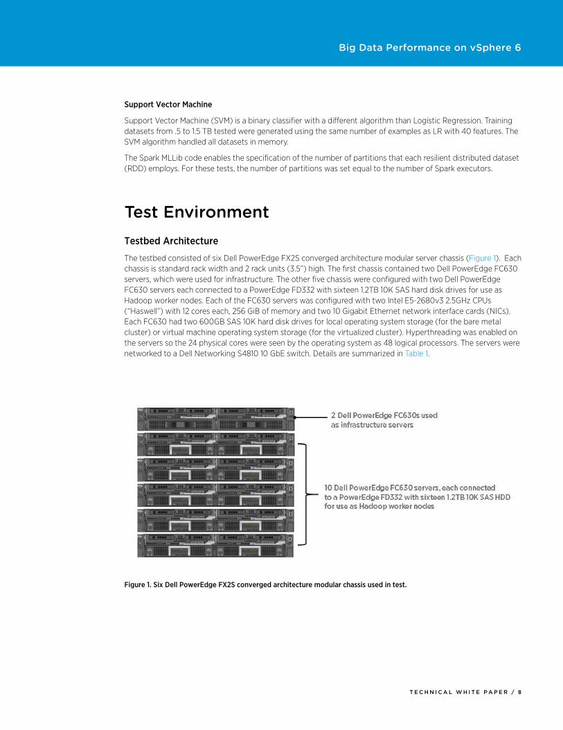
The testbed consisted of six Dell PowerEdge FX2S converged architecture modular server chassis (Figure 1). Each chassis is standard rack width and 2 rack units (3.5”) high. The first chassis contained two Dell PowerEdge FC630 servers, which were used for infrastructure. The other five chassis were configured with two Dell PowerEdge FC630 servers each connected to a PowerEdge FD332 with sixteen 1.2TB 10K SAS hard disk drives for use as Hadoop worker nodes. Each of the FC630 servers was configured with two Intel E5-2680v3 2.5GHz CPUs (“Haswell”) with 12 cores each, 256 GiB of memory and two 10 Gigabit Ethernet network interface cards (NICs). Each FC630 had two 600GB SAS 10K hard disk drives for local operating system storage (for the bare metal cluster) or virtual machine operating system storage (for the virtualized cluster). Hyperthreading was enabled on the servers so the 24 physical cores were seen by the operating system as 48 logical processors. The servers were networked to a Dell Networking S4810 10 GbE switch. Details are summarized in Table 1.

Figure 1. Six Dell PowerEdge FX2S converged architecture modular chassis used in test.



COMPONENT QUANTITY/TYPE

Server Dell PowerEdge FC630

Processor 2x Intel E5-2680v3 2.5GHz CPUs w/ 12 cores each

Logical Processors (including hyperthreads)

48

Memory 256 GiB

NICs Intel X520k dual-port 10GbE NICs

Internal Disk Drives 2x 600GB SAS 10K HDD

Direct Attached Disk Drives

(worker nodes only)

PowerEdge FD332 w/ 16x 1.2TB 10K SAS HDD

RAID Controller Dell PERC 730P

Remote Access Integrated Dell Remote Access Controller 8 (iDRAC)

Table 1. Server configuration. In this document notation such as “GiB” refers to binary quantities such as gigibytes (2**30 or 1,073,741,824) while “GB” refers to gigabytes (10**9 or 1,000,000,000).

Hardware

VMware vSphere ESXi version 6.0.0 was installed on an SD card on each server. The two internal 600GB disks in each server were mirrored in a RAID1 set and used for the operating system (for bare metal) or as a virtual machine file system (VMFS) datastore upon which the operating system disks for the virtual machines on that host were stored. The sixteen 1.2 TB drives attached to each worker server were used as data drives. For the bare metal cluster, the drives were formatted and mounted as an ext4 filesystem. For the virtualized cluster, they were set up as VMFS datastores with one 1.1 TB virtual machine disk (VMDK) created on each, which was then formatted and mounted as ext4 using the same parameters as in the bare metal case. For best performance, these VMDKs were initialized with eager-zeroed thick formatting, meaning that the disk was pre-formatted so writes did not have to format the disk during production.

One virtual switch was created on each ESXi host using the two 10 GbE NICs bonded together. This switch served as the management network for the host as well as the external virtual machine network for the guests. By setting the bond load balancing policy to Route based on originating virtual port, both failover and performance throughput enhancement were achieved because the virtual machines attached to that NIC bond had different originating ports. The maximum transmission unit (MTU) of the bonded 10GbE NIC was set to 9000 bytes to handle jumbo Ethernet frames (the guest NIC must be set the same way).

In a Hadoop cluster, there are three kinds of servers or nodes (see Table 2). One or more gateway servers act as client systems for Hadoop applications and provide a remote access point for users of cluster applications. Master servers run the Hadoop master services such as NameNode and ResourceManager and their associated services (JobHistory Server, etc.), as well as other Hadoop services such as Hive, Oozie, and Hue. Worker nodes run only the resource intensive HDFS DataNode role and the YARN NodeManager role (which also serve as Spark executors). For NameNode and ResourceManager high availability, at least three ZooKeeper services and three HDFS JournalNodes are required; these can run on the gateway and two master servers. The Active NameNode and ResourceManager run on different nodes for best distribution of CPU load, with the Standby of each on the opposite master node. The Master1 and Master2 virtual machines should be placed on different servers for availability.

T E C H N I C A L W H I T E P A P E R / 1 0


NODE ROLES

Gateway Cloudera Manager, ZooKeeper Server, HDFS JournalNode, HDFS gateway, YARN gateway, Hive gateway, Spark gateway

Master1 HDFS NameNode (Active), YARN ResourceManager (Standby), ZooKeeper Server, HDFS JournalNode, HDFS Balancer, HDFS FailoverController, HDFS HttpFS, HDFS NFS gateway

Master2 HDFS NameNode (Standby), YARN ResourceManager (Active), ZooKeeper Server, HDFS JournalNode, HDFS FailoverController, YARN JobHistory Server, Hive Metastore Server, Hive Server2, Hive WebHCat Server, Hue Server, Oozie Server, Spark History Server

Workers (40) HDFS DataNode, YARN NodeManager, Spark Executor

Table 2. Hadoop/Spark roles

In these tests, two of the virtualized servers acted as the infrastructure cluster, hosting the gateway and two master servers as well as Cloudera Manager, vSphere vCenter Server, and two VMware management tools: vRealize Operations Manager Appliance and vRealize Log Insight. These services can be protected and load balanced through VMware High Availability and Distributed Resource Scheduler, in addition to the protection offered by NameNode and ResourceManager high availability. These are the only servers that need direct network access to the outside world so they can be protected with a firewall and access limited with a tool such as Kerberos. (The worker nodes may need Internet access during installation depending on the method used; that can be achieved by IP forwarding through one of the master servers).

The other ten virtualized servers hosted worker nodes. Following the best practices described above, 4 virtual machines were created on each vSphere host to optimize NUMA locality and at the same time present an optimum number of disks, 4, to each node. The 48 virtual CPUs on each host (corresponding to the 48 logical processors with hyperthreading enabled) were exactly committed to the 4 virtual machines at 12 each. Again, following best practices, 16 GiB of each server’s 256 GiB of memory (6%) was provided for ESXi, and the remaining 240 GiB was divided equally as 60 GiB to each virtual machine. On all virtual machines, the virtual NIC connected to the bonded 10 GbE NIC was assigned an IP address internal to the cluster. The vmxnet3 driver was used for all network connections.

Each virtual machine had its operating system drive on the RAID1 datastore for that host and four 1.1 TB VMDKs set up as data disks. All disks were connected through virtual SCSI controllers using the VMware Paravirtual SCSI driver. The OS disk and the first data disk utilized SCSI controller 0, while data disks 2, 3, and 4 utilized SCSI controllers 1, 2, and 3 respectively. The virtualized cluster is shown in Figure 2.



Virtualized Cluster

Figure 2. Big Data cluster – virtualized

For the bare metal performance tests, the worker nodes were reinstalled with CentOS 6.7. The same infrastructure as used in the vSphere tests was used in the bare metal tests. This ensures a fair comparison of 10 virtualized worker servers vs. 10 bare metal worker servers while not penalizing the bare metal side of the comparison by dedicating 3 full servers for Hadoop master nodes, ZooKeeper, etc. It is a common practice in production clusters to have a dedicated infrastructure (comprised of less expensive servers) managing several clusters of more richly configured worker servers.

Each of the 10 bare metal worker nodes used the full complement of 48 logical processors, 256 GiB, one RAID1 pair of 600GB disks for its operating system, and 16 1.1 TB data disks. The two 10 GbE NICs were bonded together using Linux bonding mode 6 (adaptive load balancing) to provide both failover and enhanced throughput similar to that employed with ESXi. In neither the virtualized nor the bare metal case was the network switch to which the NICs attach configured with any special configuration for the NIC bonding. The bare metal cluster is shown in Figure 3.

The worker node configurations for virtualized and bare metal are compared in Table 3. Container memory and vcores are discussed in more detail below.



Bare Metal Cluster

Figure 3. Big Data cluster - bare metal

COMPONENT VM BARE METAL

Virtual CPUs 12 48

Memory 60 GiB 256 GiB

Container Memory 42 GiB 204 GiB

Container vcores 12 48

Virtual NICs Bonded 10 GbE NICs – ESX bonding Bonded 10 GbE NICs – Balance ALB

Disk Drives 1x 40 GB OS disk, 4x 1.1 TB data disks 1x 600 GB OS disk, 16x 1.1 TB data disks

Table 3. Worker node configuration - VMs vs. bare metal



Software

The software stack employed on each virtual machine is shown in Table 4. The combination of Cloudera Distribution of Hadoop (CDH) 5.7.1 on CentOS 6.7 was used. The Oracle Java Development Kit 1.8.0_65 was installed on each node and then employed by CDH. MySQL 5.7 Community Release was installed on Master 2 for the Hive Metastore and Oozie databases.

COMPONENT VERSION

vSphere 6.0.0

Guest Operating System Centos 6.7

Cloudera Distribution of Hadoop 5.7.1

Cloudera Manager 5.7.1

Hadoop 2.6.0+cdh5.7.1+1335

HDFS 2.6.0+cdh5.7.1+1335

YARN 2.6.0+cdh5.7.1+1335

MapReduce2 2.6.0+cdh5.7.1+1335

Hive 1.1.0+cdh5.7.1+564

Spark 1.6.0+cdh5.7.1+193

ZooKeeper 3.4.5+cdh5.7.1+93

Java Oracle 1.8.0_65

MySQL 5.6 Community Release

Table 4. Key software components

Hadoop/Spark Configuration

The Cloudera Distribution of Hadoop (CDH) was installed using Cloudera Manager and the parcels method (see the Cloudera documentation [5] for details). HDFS, YARN, ZooKeeper, Spark, Hive, Hue, and Oozie were installed with the roles deployed as shown in Table 2. Once the Cloudera Manager and Master nodes were installed on the infrastructure servers, they were left in place for the 5- and 10-worker server virtualized clusters, as well as the 10-worker server bare metal cluster, with the worker nodes being redeployed between each set of tests. The Cloudera Manager home screen is shown in Figure 4.

http://www.cloudera.com/documentation/enterprise/latest.html



Figure 4. Cloudera Manager screenshot showing 10 Terabyte TeraGen/TeraSort/TeraValidate resource utilization. Where the CPU hits 0% marks the beginning of the next application.

A final cluster optimization is to use the Hadoop concept of rack awareness to label virtual machines running on the same host as belonging to the same “rack.” This not only ensures that the multiple replicas of a given block are placed on different physical servers for availability, but that a process running on one virtual machine that requires a given block will copy that block from a virtual machine on the same rack if possible. Since that block is actually on the same physical server, copy time will be minimized.

As described above in tuning for Hadoop, the two key cluster parameters that need to be set by the user are yarn.nodemanager.resource.cpu-vcores and yarn.nodemanager.resource.memory-mb, which tell YARN how much CPU and memory resources, respectively, can be allocated to task containers in each worker node.

For the virtualized case, the 12 vCPUs in each worker VM were exactly committed to YARN containers. As seen in Figure 5, this actually overcommits the CPUs slightly since, in addition to the 12 vcores for containers, a total of 1 vcore was required for the DataNode and NodeManager processes that run on each worker node. For the bare metal case, all 48 logical CPUs were allocated to containers, again slightly overcommitting the CPU resources.

The memory calculation was a little more involved. Each of the four worker virtual machines per host have 60 GiB of memory after the 16 GiB of the 256 GiB host memory was set aside for ESXi. Cloudera Manager then allocated 20% of that 60 GiB for the virtual machine’s operating system. Of the remaining 48 GiB, 1.3 GiB each were required for the Java Virtual Machines (JVMs) running the DataNode and NodeManager processes, plus 4 GiB for cache, leaving about 42 GiB for containers. This left the amount of memory for the operating system slightly under Cloudera’s target of 20%. Since no swapping was seen on the worker nodes, the warning from Cloudera Manager was suppressed. (The 20% target could have been lowered as well).



Figure 5. DataNode/NodeManager resources

The memory calculation for the bare metal servers is similar. Setting aside 20% of the 256 GiB server memory for the OS plus the 6.6 GiB for the DataNode and NodeManager processes and cache leaves about 198 GiB for containers, which was adjusted upward slightly to 204 GiB, again without seeing any swapping.

Note that between the ESXi overhead (16 GiB) and the fact that 4 sets of JVMs for the DataNode, NodeManager, and associated cache (requiring 6.6 GiB total) occur on the 4 virtual machines versus just 1 set on bare metal, the total container memory of the 4 virtual machines per host (168 GiB) is lower than that available on the same host without virtualization (204) (see Figure 6). However, as will be shown in the results, this advantage does not make up for the virtualization advantages of NUMA locality and better disk utilization on most applications.

Figure 6. Worker node memory use - virtualized vs. bare metal

To achieve the correct balance between number and size of containers, much experimentation was done, particularly with TeraSort, factoring in the available memory vs. vcores. For the virtualized workers, the total 12 vcores for containers limits the number of map tasks to 12 (with mapreduce.map.cpu.vcores set to 1), so the entire 42 GiB of memory was allocated by setting mapreduce.map.cpu.memory.mb to 42 divided by 12 or 3.5 GiB. Reduce tasks, which generally require more memory than map tasks, were found to be able to use 2 vcores each, so mapreduce.map.cpu.vcores was set to 2 and mapreduce.map.cpu.memory.mb was set to 7 GiB so that 6 reduce tasks take up both the 12 vcores and 42 GiB of container memory.

0

16

45.4

45.6

6.6

26.4

204

168

0 50 100 150 200 250 300

Bare Metal

Virtualized

GiB

Memory Use Virtualized vs. Bare Metal

ESXi

OS

DN/NM

Container



The bare metal cluster is limited to the same overall number of vcores; that is, a single bare metal host has 48 vcores for containers, the same total as the 4 virtual machines that ran on it in the virtualized tests. So the same vcore allocation to map and reduce tasks was used. However, the slightly larger memory available on the bare metal servers enabled the map and reduce tasks to be allocated more memory, 4.25 and 8.5 GiB, respectively.

It should be emphasized this type of task specification differs from the MapReduce1 notion of map and reduce slots. With MapReduce1 the pre-defined map and reduce slots could only be used for each type of task, so during the map- and reduce-only stages of applications, the cluster was underutilized. With YARN and the parameter set specified here, the full resources of the cluster will be devoted to the map-only stages of applications and then re-deployed to the reduce stage. During the transition period, YARN will allocate resources to map or reduce tasks as resources are available during task initiation.

As mentioned earlier, Spark executors optimally use larger memory footprints. Thus spark.executor.memory was set to 8 GiB with spark.yarn.executor.memoryOverhead set to 2 GiB for a total of 10 GiB on the virtualized cluster. Three vcores were allocated to executors with spark.executor.cores, so each virtualized node can support a maximum of 4 executors (with 2 GiB of container memory left over). On bare metal the optimum point was found to be 10 GiB for the executor plus 2 GiB overhead, and 3 vcores. Sixteen executors can run on each bare metal server, also with some memory left over.

The log levels of all key processes were turned down from the Cloudera default of INFO to WARN for production use, but the much lower levels of log writes did not have a measurable impact on application performance.

All parameters are summarized in Table 5.

PARAMETER DEFAULT VIRTUALIZED BARE METAL

dfs.blocksize 128 MiB 256 MiB 256 MiB

mapreduce.task.io.sort.mb 256 MiB 400 MiB 400 MiB

yarn.nodemanager.resource.cpu-vcores 12 48

mapreduce.map.cpu.vcores 1 1 1

mapreduce.reduce.cpu.vcores 1 2 2

yarn.nodemanager.resource.memory-mb 42 GiB 204 GiB

mapreduce.map.memory.mb 1 GiB 3.5 GiB 4.25 GiB

mapreduce.reduce.memory.mb 1 GiB 7 GiB 8.5 GiB

Maximum map tasks per node 12 48

Maximum reduce tasks per node 6 24

spark.executor.cores 1 3 3

spark.executor.memory 256 MiB 8 GiB 1 0 GiB

spark.yarn.executor.memoryOverhead 26 MiB 2 GiB 2 GiB

Maximum number of Spark executors per node 4 16

Log Level on HDFS, YARN, Hive INFO WARN WARN

Note: MiB = 2**20 (1048576) bytes, GiB = 2**30 (1073741824) bytes

Table 5. Key Hadoop/Spark cluster parameters used in tests



Performance Results – Virtualized vs Bare Metal For all configurations, the number of map tasks was specified for the TeraGen test, the number of reduce tasks was specified for TeraSort, and the number of executors was specified for all Spark tests. In all cases, the full number of tasks the cluster can handle was specified. For map tasks, each of the 40 worker virtual machines can handle 12 tasks, for a total of 480. However, one task needs to be devoted to the ApplicationMaster that runs each application, so 479 map tasks were specified for TeraGen using mapreduce.job.maps in the TeraGen command line. Similarly, 239 of the fatter reduce tasks were specified for TeraSort using mapreduce.job.reduces, and 159 Spark executors were specified in the Spark command line. The numbers for the bare metal cluster are the same, as noted above, since the total vcore count per server is the same (but the tasks on bare metal are allocated more memory). See Table 6 for all cases.

METRIC 5 HOSTS

VIRTUALIZED

10 HOSTS VIRTUALIZED 10 HOSTS BARE METAL

Worker nodes 20 40 10

Total container vcores 240 480 480

Total container memory 840 GiB 1680 GiB 2040 GiB

Maximum map tasks per node 12 12 48

Maximum reduce tasks per node 6 6 24

Maximum number of Spark executors per node

4 4 16

Total number of containers available for Map tasks

240 480 480

Total number of containers available for Reduce tasks

120 240 240

Total number of containers available for Spark Executors

80 160 160

Table 6. 5- and 10-host total containers available per task. In each case the number of tasks specified for the cluster must be these numbers reduced by 1, for the ApplicationMaster.

TeraSort Results

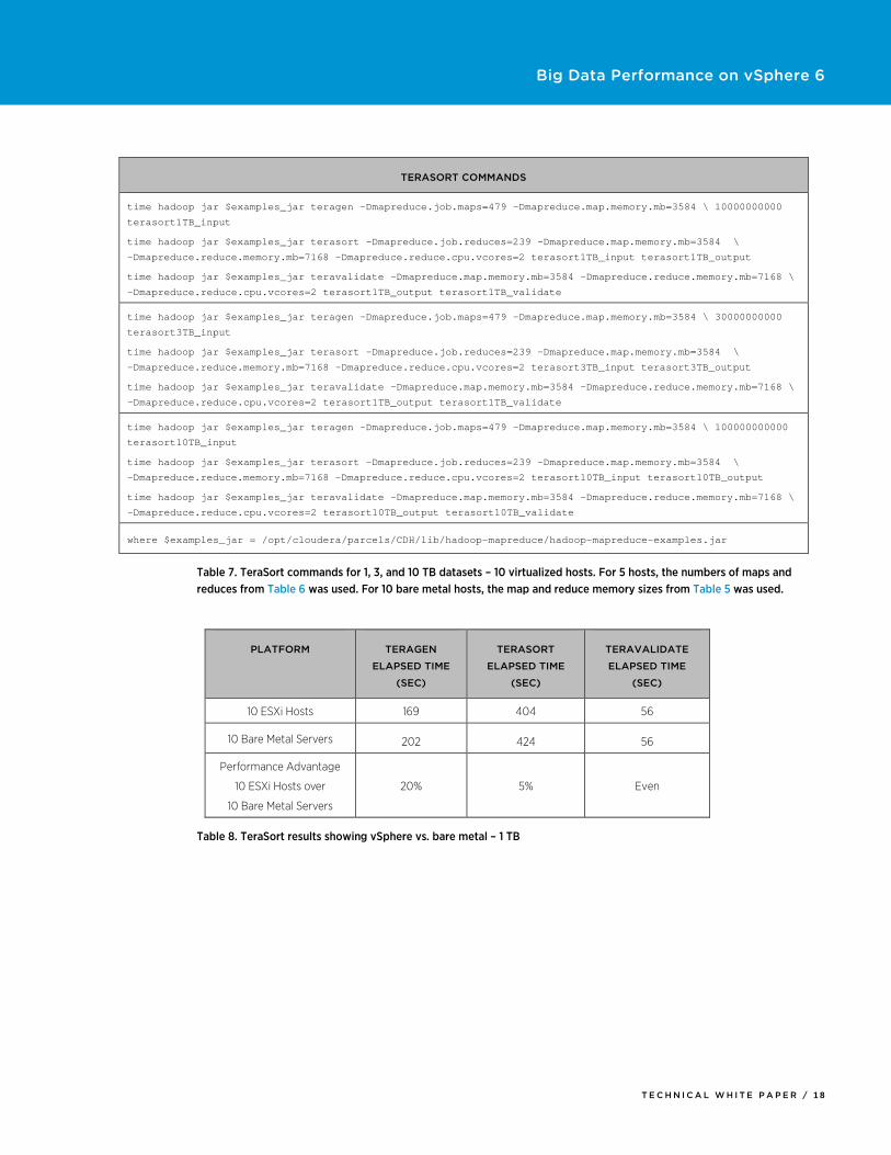
The TeraSort suite was run with the cluster parameters shown in Table 5 and the command lines of the form shown in Table 7. The results are shown in Table 8−Table 10 and plotted in Figure 7. Virtualized TeraGen was faster than bare metal due to the smaller number of disks per data node. This tends to even out over time (1 TB virtualized is 20% faster, 10 TB virtualized is 4% faster). Virtualized TeraSort is about 5% faster than bare metal due to the benefits of NUMA locality discussed above. Virtualized TeraValidate, mainly reads, is about the same as bare metal.

The resource utilization of the three applications is shown in the Cloudera Manager screenshot in Figure 4. During TeraGen, about 19 GiB per second (GB/s) of cluster disk writes occur accompanied by over 10 GB/s of cluster network I/O as replicas are copied to other nodes. TeraSort starts with the CPU-intensive map sort, with disk writes occurring as sorted data is spilled to disk. In the reduce copy phase of TeraSort, network I/O ticks up, followed by disk I/O as the sorted data gets written to HDFS by the reducers. Finally, TeraValidate is a high disk read, low CPU operation.



TERASORT COMMANDS

time hadoop jar $examples_jar teragen -Dmapreduce.job.maps=479 -Dmapreduce.map.memory.mb=3584 \ 10000000000

terasort1TB_input

time hadoop jar $examples_jar terasort -Dmapreduce.job.reduces=239 -Dmapreduce.map.memory.mb=3584 \

-Dmapreduce.reduce.memory.mb=7168 -Dmapreduce.reduce.cpu.vcores=2 terasort1TB_input terasort1TB_output

time hadoop jar $examples_jar teravalidate -Dmapreduce.map.memory.mb=3584 -Dmapreduce.reduce.memory.mb=7168 \

-Dmapreduce.reduce.cpu.vcores=2 terasort1TB_output terasort1TB_validate


terasort3TB_input






terasort10TB_input





where $examples_jar = /opt/cloudera/parcels/CDH/lib/hadoop-mapreduce/hadoop-mapreduce-examples.jar

Table 7. TeraSort commands for 1, 3, and 10 TB datasets – 10 virtualized hosts. For 5 hosts, the numbers of maps and reduces from Table 6 was used. For 10 bare metal hosts, the map and reduce memory sizes from Table 5 was used.

PLATFORM TERAGEN

ELAPSED TIME

(SEC)

TERASORT

ELAPSED TIME

(SEC)

TERAVALIDATE

ELAPSED TIME

(SEC)

10 ESXi Hosts 169 404 56

10 Bare Metal Servers 202 424 56

Performance Advantage

10 ESXi Hosts over

10 Bare Metal Servers

20% 5% Even

Table 8. TeraSort results showing vSphere vs. bare metal – 1 TB



PLATFORM TERAGEN

ELAPSED TIME

(SEC)

TERASORT

ELAPSED TIME

(SEC)

TERAVALIDATE

ELAPSED TIME

(SEC)

10 ESXi Hosts 484 1265 288

10 Bare Metal Servers 550 1365 NA


10 ESXi Hosts over


14% 8%


PLATFORM TERAGEN

ELAPSED TIME

(SEC)

TERASORT

ELAPSED TIME

(SEC)

TERAVALIDATE

ELAPSED TIME

(SEC)

10 ESXi Hosts 1676 4274 872



10 ESXi Hosts over


4% 5% 1% slower


Figure 7. TeraSort suite performance showing vSphere vs. bare metal

0

500

1000

1500

2000

2500

3000

3500

4000

4500

5000

TeraGen(1TB)

TeraSort(1TB)

TeraValidate(1TB)

TeraGen(3TB)

TeraSort(3TB)

TeraValidate(3TB)

TeraGen(10TB)

TeraSort(10TB)

TeraValidate(10TB)

Elap

sed

Tim

e (s

ec)

TeraSort Suite Performance - vSphere vs. Bare Metal Smaller is Better

10 ESXi hosts 10 Bare Metal Servers



TestDFSIO Results

TestDFSIO was used as shown in Table 11 to generate output of 1, 3, and 10 TB by writing an increasing number of 10 GB files. The results are shown Table 12 and Figure 8. Like TeraGen, TestDFSIO was faster on the virtualized cluster due to the better match of number of disks (4) to DataNodes than on bare metal (16). The generation of the 3 and 10 TB outputs were about 10% faster than bare metal, with the virtualized cluster seeing 20.4 GiB/s maximum cluster disk I/O vs. 16.8 for bare metal.

TESTDFSIO COMMANDS

time hadoop jar $test_jar TestDFSIO -Dmapreduce.map.memory.mb=3584 -Dmapreduce.reduce.memory.mb=7168 \ -Dmapreduce.reduce.cpu.vcores=2 -write -nrFiles 100 -size 10GB

time hadoop jar $test_jar TestDFSIO -Dmapreduce.map.memory.mb=3584 -Dmapreduce.reduce.memory.mb=7168 \ -Dmapreduce.reduce.cpu.vcores=2 -write -nrFiles 300 -size 10GB

time hadoop jar $test_jar TestDFSIO -Dmapreduce.map.memory.mb=3584 -Dmapreduce.reduce.memory.mb=7168 \

-Dmapreduce.reduce.cpu.vcores=2 -write -nrFiles 1000 -size 10GB

where $test_jar=/opt/cloudera/parcels/CDH/lib/hadoop-mapreduce/hadoop-mapreduce-client-jobclient-tests.jar

Table 11. TestDFSIO commands for 1, 3, and 10 TB datasets for the virtualized clusters. For 10 bare metal hosts the map and reduce memory sizes from Table 5 was used.

PLATFORM TESTDFSIO 1TB

ELAPSED TIME

(SEC)

TESTDFSIO 3TB

ELAPSED TIME

(SEC)

TESTDFSIO 10TB

ELAPSED TIME

(SEC)

10 ESXi Hosts 176 543 1683



10 ESXi Hosts over


42% 9% 10%

Table 12. TestDFSIO results showing vSphere vs. bare metal



Figure 8. TestDFSIO performance showing vSphere vs. bare metal

Spark Results

The Spark Support Vector Machines (SVM) and Logistic Regression (LR) machine learning programs were driven by SparkBench code from the SparkTC github project [4]. For each test, first a training set of the specified size was created. Then the machine learning component was executed and timed, with the training set ingested and used to build the mathematical model to be used to classify real input data. SVM results are shown in Table 13 and Figure 9. For SVM, which stays in memory even for the larger dataset sizes, the larger memory of the bare metal Spark executors was more than offset by the NUMA locality advantage of the virtualized ones, so SVM ran about 10% faster virtualized. The advantage seems to drop off slightly with an increased dataset size, perhaps showing the influence of the larger bare metal executor memory.

Table 13. Spark Support Vector Machine results showing vSphere vs. bare metal

0

200

400

600

800

1000

1200

1400

1600

1800

2000

TestDFSIO (1TB) TestDFSIO (3TB) TestDFSIO (10TB)

Elap

sed

Tim

e (s

ec)

TestDFSIO Performance - vSphere vs Bare Metal Smaller Is Better

10 ESXi Hosts 10 Bare Metal Servers

PLATFORM SVM .5 TB

ELAPSED TIME

(SEC)

SVM 1 TB

ELAPSED TIME

(SEC)

SVM 1.5 TB

ELAPSED TIME

(SEC)

10 ESXi Hosts 278 711 1280



10 ESXi Hosts over


12% 10% 8%



Figure 9. Spark Support Vector Machine performance

Logistic Regression was run with two different numbers of features, 40 and 80, to be able to generate dataset sizes up to 3 TB that would be much larger than the available container memory. The results are shown in Table 14 and Table 15 and Figure 10. Unlike SVM, the LR resilient distributed datasets were written to disk during processing as they filled up container memory. Despite the virtualized disk I/O advantage seen in the MapReduce tests, the virtualized LR tests actually ran slightly slower than bare metal for the larger dataset sizes. This needs further examination. Perhaps the caching to disk needed better tuning or the large number of features exceeded the size the algorithm was designed to handle.

Table 14. Spark Logistic Regression results (40 features) showing vSphere vs. bare metal

0

200

400

600

800

1000

1200

1400

1600

SVM (.5TB) SVM (1TB) SVM (1.5TB)

Elap

sed

Tim

e (s

ec)

Spark Support Vector Machine Perf - vSphere vs. Bare Metal Smaller Is Better

Results shown for 40 features with 700M, 1.4B and 2.1B examples

10 ESXi Hosts 10 Bare Metal Servers

PLATFORM LOGISTIC

REGRESSION

40 FEATURES

.5 TB

ELAPSED TIME

(SEC)

LOGISTIC

REGRESSION

40 FEATURES

1 TB

ELAPSED TIME

(SEC)

LOGISTIC

REGRESSION

40 FEATURES

1.5 TB

ELAPSED TIME

(SEC)

10 ESXi Hosts 129 217 334



10 ESXi Hosts over


1% 3% 4% slower



Table 15. Spark Logistic Regression results (80 features) showing vSphere vs. bare metal

Figure 10. Spark Logistic Regression performance showing vSphere vs. bare metal

0

100

200

300

400

500

600

700

LR-40F(.5TB)

LR -40F(1TB)

LR-40F(1.5TB)

LR-80F (1TB) LR -80F(2TB)

LR-8F (3TB)

Elap

sed

Tim

e (s

ec)

Spark Logistic Regression Performance - vSphere vs. Bare MetalSmaller Is Better

Results shown for 40 and 80 features with 700M, 1.4B and 2.1B examples

10 ESXi hosts 10 Bare Metal Servers

PLATFORM LOGISTIC

REGRESSION

80 FEATURES

1 TB

ELAPSED TIME

(SEC)

LOGISTIC

REGRESSION

80 FEATURES

2 TB

ELAPSED TIME

(SEC)

LOGISTIC

REGRESSION

80 FEATURES

3 TB

ELAPSED TIME

(SEC)

10 ESXi Hosts 209 426 663



10 ESXi Hosts over


5% 3% slower 1% slower



Performance Results – Scaling from 5 to 10 Hosts To measure the scalability of the virtualized cluster, all of the tests were repeated with half of the worker nodes using the application parameters described above. As the remaining charts and graphs show (which use the same 10 ESXi host data as above), all of the tests scaled well as the worker nodes increased from 5 hosts to 10 hosts. Most of the scaling numbers were around 2x, which would indicate linear scaling, with a few outliers as low as 1.74x and as high as 2.85x. Additionally, as seen on the graphs, each application scaled well on both 5 and 10 hosts as the dataset size increased.

TeraSort Results

PLATFORM TERAGEN

ELAPSED TIME

(SEC)

TERASORT

ELAPSED TIME

(SEC)

TERAVALIDATE

ELAPSED TIME

(SEC)

5 ESXi Hosts 323 709 139

10 ESXi Hosts 169 404 56

Scaling 5 to 10 ESXi Hosts 1.91x 2.50x 2.48x

Table 16. TeraSort results showing scaling from 5 hosts to 10 hosts - 1 TB

PLATFORM TERAGEN

ELAPSED TIME

(SEC)

TERASORT

ELAPSED TIME

(SEC)

TERAVALIDATE

ELAPSED TIME

(SEC)

5 ESXi Hosts 995 2438 530

10 ESXi Hosts 484 1265 288


Table 17. TeraSort results showing scaling from 5 hosts to 10 hosts – 3 TB



PLATFORM TERAGEN

ELAPSED TIME

(SEC)

TERASORT

ELAPSED TIME

(SEC)

TERAVALIDATE

ELAPSED TIME

(SEC)

5 ESXi Hosts 3327 8357 2376

10 ESXi Hosts 1676 4274 872


Table 18. TeraSort results showing scaling from 5 hosts to 10 hosts – 10 TB

Figure 11. TeraSort suite performance

0

1000

2000

3000

4000

5000

6000

7000

8000

9000

TeraGen(1TB)

TeraSort(1TB)

TeraValidate(1TB)

TeraGen(3TB)

TeraSort(3TB)

TeraValidate(3TB)

TeraGen(10TB)

TeraSort(10TB)

TeraValidate(10TB)

Elap

sed

Tim

e (s

ec)

TeraSort Suite Performance - Scaling from 5 to 10 Hosts - Smaller Is Better

5 ESXi Hosts 10 ESXi hosts



TestDFSIO Results

PLATFORM TESTDFSIO 1TB

ELAPSED TIME

(SEC)

TESTDFSIO 3TB

ELAPSED TIME

(SEC)

TESTDFSIO 10TB

ELAPSED TIME

(SEC)

5 ESXi Hosts 381 1209 3669

10 ESXi Hosts 176 543 1683


Table 19. TestDFSIO results showing scaling from 5 hosts to 10 hosts

Figure 12. TestDFSIO performance showing scaling from 5 hosts to 10 hosts

0

500

1000

1500

2000

2500

3000

3500

4000

TestDFSIO (1TB) TestDFSIO (3TB) TestDFSIO (10TB)

Elap

sed

Tim

e (s

ec)

TestDFSIO Performance - Scaling from 5 to 10 Hosts Smaller Is Better

5 ESXi Hosts 10 ESXi Hosts



Spark Results

PLATFORM SVM .5 TB

ELAPSED TIME

(SEC)

SVM 1 TB

ELAPSED TIME

(SEC)

5 ESXi Hosts 673 1931

10 ESXi Hosts 278 711

Scaling 5 to 10 ESXi Hosts 2.16x 2.23x

Table 20. Spark Support Vector Machine results showing scaling from 5 hosts to 10 hosts

Figure 13. Spark Scalable Vector Machine performance showing scaling from 5 hosts to 10 hosts

0

500

1000

1500

2000

2500

SVM (.5TB) SVM (1TB)

Elap

sed

Tim

e (s

ec)

Spark Support Vector Machine Perf - Scaling from 5 to 10 Hosts Smaller Is Better

Results shown for 40 features with 700M and 1.4B examples

5 ESXi Hosts 10 ESXi Hosts



Table 21. Spark Logistic Regression (40 features) results showing scaling from 5 hosts to 10 hosts

PLATFORM LOGISTIC REGRESSION 80 FEATURES

1 TB ELAPSED TIME

(SEC)

LOGISTIC REGRESSION 80 FEATURES

2 TB ELAPSED TIME

(SEC)

LOGISTIC REGRESSION 80 FEATURES

3 TB ELAPSED TIME

(SEC)

5 ESXi Hosts 423 1134 1888

10 ESXi Hosts 209 426 663


Table 22. Spark Logistic Regression (80 features) results showing scaling from 5 hosts to 10 hosts

PLATFORM LOGISTIC

REGRESSION

40 FEATURES

.5 TB

ELAPSED TIME

(SEC)

LOGISTIC

REGRESSION

40 FEATURES

1 TB

ELAPSED TIME

(SEC)

LOGISTIC

REGRESSION

40 FEATURES

1.5 TB

ELAPSED TIME

(SEC)

5 ESXi Hosts 223 451 859

10 ESXi Hosts 129 217 334




Figure 14. Spark Logistic Regression performance showing scaling from 5 hosts to 10 hosts

Best Practices To recap, here are the best practices cited in this paper:

• Reserve about 5-6% of total server memory for ESXi; use the remainder for the virtual machines.

• Create 1 or more virtual machines per NUMA node.

• Limit the number of disks per DataNode to maximize the utilization of each disk – 4 to 6 is a good starting point.

• Use eager-zeroed thick VMDKs along with the ext4 filesystem inside the guest.

• Use the VMware Paravirtual SCSI (pvscsi) adapter for disk controllers; use all 4 virtual SCSI controllers available in vSphere 6.0.

• Use the vmxnet3 network driver; configure virtual switches with MTU=9000 for jumbo frames.

• Configure the guest operating system for Hadoop performance including enabling jumbo IP frames, reducing swappiness, and disabling transparent hugepage compaction.

• Place Hadoop master roles, ZooKeeper, and journal nodes on three virtual machines for optimum performance and to enable high availability.

• Dedicate the worker nodes to run only the HDFS DataNode, YARN NodeManager, and Spark Executor roles.

• Use the Hadoop rack awareness feature to place virtual machines belonging to the same physical host in the same rack for optimized HDFS block placement.

• Run the Hive Metastore in a separate MySQL database.

• Set the Yarn cluster container memory and vcores to slightly overcommit both resources.

• Adjust the task memory and vcore requirement to optimize the number of maps and reduces for each application.

0200400600800

100012001400160018002000

LR-40F(.5TB)

LR -40F(1TB)

LR-40F(1.5TB)

LR-80F(1TB)

LR -80F(2TB)

LR-8F (3TB)

Elap

sed

Tim

e (s

ec)

Spark Logistic Regression Performance Scaling from 5 to 10 Hosts

Smaller Is BetterResults shown for 40 and 80 features with 700M, 1.4B, and 2.1B examples

5 ESXi Hosts 10 ESXi hosts



Conclusion Virtualization of Big Data clusters with vSphere brings advantages that bare metal clusters don’t have including better utilization of cluster resources, enhanced operational flexibility, and ease of deployment and management. From a performance point of view, enhanced NUMA locality and a better match of disk drives per worker node more than outweigh the extra memory required for virtualization. Through application of best practices throughout the hardware and software stack, it is possible to utilize all the benefits of virtualization without sacrificing performance in a production cluster. These best practices were tested in a highly available 12-server cluster running Hadoop MapReduce version 2 and Spark on YARN with the latest cluster management tools. Several MapReduce and Spark tests ran at 5-10% faster on vSphere than on bare metal, over a wide range of dataset sizes. One Spark test, which possibly was pushing the limits of its machine learning algorithm, ran slightly slower virtualized at higher dataset sizes.

References [1] Jeff Buell. (2015, February) Virtualized Hadoop Performance with VMware vSphere 6.


[2] The Apache Software Foundation. (2015, June) Apache Hadoop NextGen MapReduce (YARN). https://hadoop.apache.org/docs/r2.7.1/hadoop-yarn/hadoop-yarn-site/YARN.html

[3] Cloudera. (2016) Performance Management. http://www.cloudera.com/documentation/enterprise/latest/topics/admin_performance.html

[4] GitHub, Inc. (2016, June) spark-bench. https://github.com/SparkTC/spark-bench

[5] Cloudera. (2016) Cloudera Enterprise 5.8.x Documentation. http://www.cloudera.com/documentation/enterprise/latest.html


https://hadoop.apache.org/docs/r2.7.1/hadoop-yarn/hadoop-yarn-site/YARN.html

http://www.cloudera.com/documentation/enterprise/latest/topics/admin_performance.html

https://github.com/SparkTC/spark-bench

http://www.cloudera.com/documentation/enterprise/latest.html

VMware, Inc. 3401 Hillview Avenue Palo Alto CA 94304 USA Tel 877-486-9273 Fax 650-427-5001 www.vmware.com Copyright © 2016 VMware, Inc. All rights reserved. This product is protected by U.S. and international copyright and intellectual property laws. VMware products are covered by one or more patents listed at http://www.vmware.com/go/patents. VMware is a registered trademark or trademark of VMware, Inc. in the United States and/or other jurisdictions. All other marks and names mentioned herein may be trademarks of their respective companies. Date: 23-Aug-16 Comments on this document: https://communities.vmware.com/docs/DOC-32739


About the Author Dave Jaffe is a staff engineer at VMware, specializing in Big Data Performance.

Acknowledgements The author would like to thank Razvan Cheveresan, Tariq Magdon-Ismail, and Justin Murray for valuable discussions, and Kris Applegate and the Dell Customer Solution Center for providing access to the test cluster.

http://www.vmware.com/go/patents

https://communities.vmware.com/docs/DOC-32739

big data performance on vsphere 6 - vmware.com€¦ · best practices are described for optimizing...

Documents