big data and business analytics - iare

LECTURE NOTES

ON

BIG DATA AND BUSINESS

ANALYTICS

2020 – 2021

VII Semester (IARE-R16)

Ms B.Pravallika, Assistant Professor

INSTITUTE OF AERONAUTICAL ENGINEERING (Autonomous)

Dundigal, Hyderabad - 500 043

Department of Information Technology

UNIT I

INTRODUCTION TO BIG DATA

1.1 INTRODUCTION TO BIG DATA

Big Data is becoming one of the most talked about technology trends nowadays. The real challenge

with the big organization is to get maximum out of the data already available and predict what kind of

data to collect in the future. How to take the existing data and make it meaningful that it provides us

accurate insight in the past data is one of the key discussion points in many of the executive meetings

in organizations.

With the explosion of the data the challenge has gone to the next level and now a Big Data is

becoming the reality in many organizations. The goal of every organization and expert is same to get

maximum out of the data, the route and the starting point are different for each organization and

expert. As organizations are evaluating and architecting big data solutions they are also learning the

ways and opportunities which are related to Big Data.

There is not a single solution to big data as well there is not a single vendor which can claim to know

all about Big Data. Big Data is too big a concept and there are many players – different architectures,

different vendors and different technology.

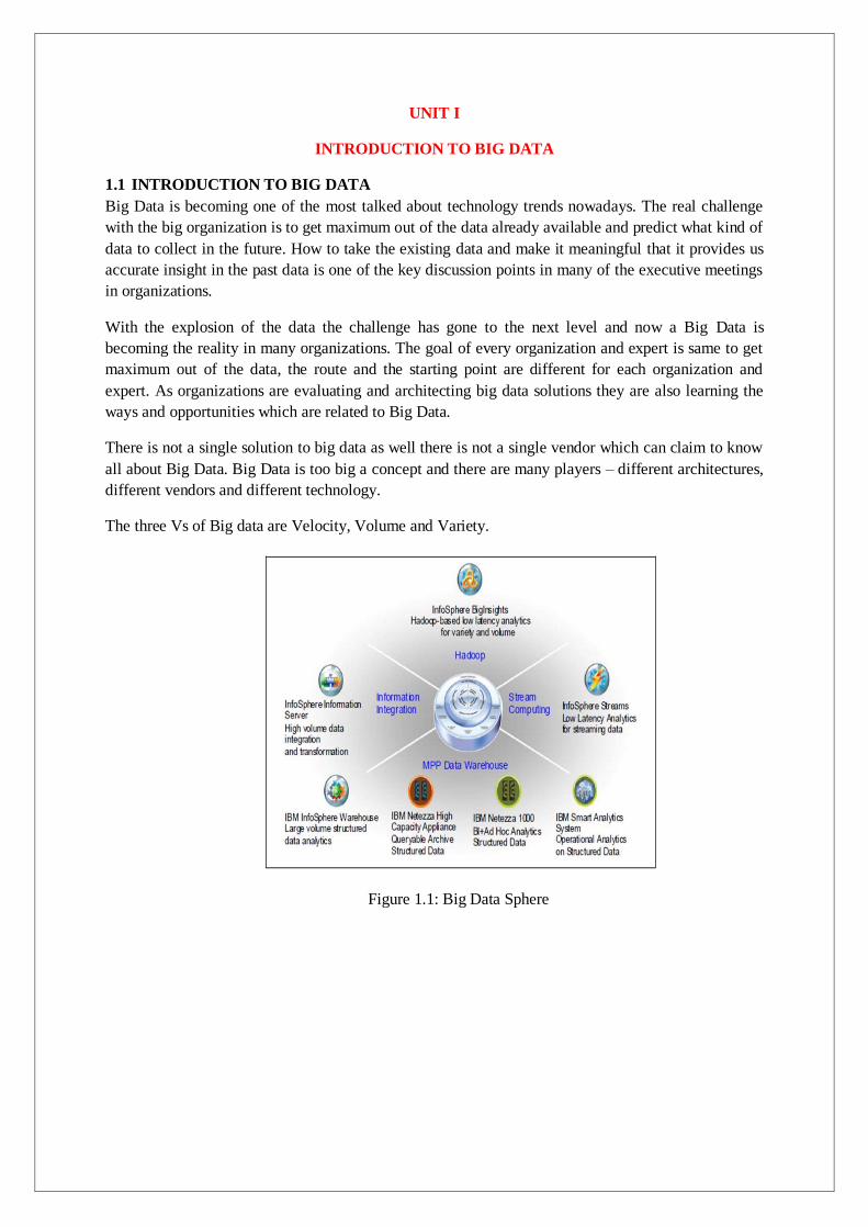
The three Vs of Big data are Velocity, Volume and Variety.

Figure 1.1: Big Data Sphere

Figure 1.2: Big Data – Transactions, Interactions, Observations

1.2 BIG DATA CHARACTERISTICS

1.The three Vs of Big data are Velocity, Volume and Variety

VOLUME

The exponential growth in the data storage as the data is now more than text data. The data can be

found in the format of videos, music’s and large images on our social media channels. It is very

common to have Terabytes and Petabytes of the storage system for enterprises. As the database

grows the applications and architecture built to support the data needs to be re-evaluated quite often.

Sometimes the same data is re-evaluated with multiple angles and even though the original data is the

same the new found intelligence creates explosion of the data. The big volume indeed represents Big

Data.

Figure

1

.

3

: Characteristics of Big

Data

VELOCITY

The data growth and social media explosion have changed how we look at the data. There was a time

when we used to believe that data of yesterday is recent. The matter of the fact newspapers is still

following that logic. However, news channels and radios have changed how fast we receive the news.

Today, people reply on social media to update them with the latest happening. On social media

sometimes a few seconds old messages (a tweet, status updates etc.) is not something interests users.

They often discard old messages and pay attention to recent updates. The data movement is now

almost real time and the update window has reduced to fractions of the seconds. This high velocity

data represent Big Data.

VARIETY

Data can be stored in multiple format. For example database, excel, csv, access or for the matter of the

fact, it can be stored in a simple text file. Sometimes the data is not even in the traditional format as

we assume, it may be in the form of video, SMS, pdf or something we might have not thought about

it. It is the need of the organization to arrange it and make it meaningful.

It will be easy to do so if we have data in the same format, however it is not the case most of the time.

The real world have data in many different formats and that is the challenge we need to overcome

with the Big Data. This variety of the data represent Big Data.

1.3TYPES OF BIG DATA

1.APACHE HADOOP

Apache Hadoop is one of the main supportive element in Big Data technologies. It simplifies the

processing of large amount of structured or unstructured data in a cheap manner. Hadoop is an open

source project from apache that is continuously improving over the years. "Hadoop is basically a set

of software libraries and frameworks to manage and process big amount of data from a single server

to thousands of machines.

Figure 1.5 : Big Data Layout

It provides an efficient and powerful error detection mechanism based on application layer rather than

relying upon hardware."

In December 2012 apache releases Hadoop 1.0.0, more information and installation guide can be

found at Apache Hadoop Documentation. Hadoop is not a single project but includes a number of

other technologies in it.

2.MAPREDUCE

MapReduce was introduced by google to create large amount of web search indexes.It is basically a

framework to write applications that processes a large amount of structured or unstructured data over

the web. MapReduce takes the query and breaks it into parts to run it on multiple nodes. By

distributed query processing it makes it easy to maintain large amount of data by dividing the data

into several different machines.Hadoop MapReduce is a software framework for easily writing

applications to manage large amount of data sets with a highly fault tolerant manner. More tutorials

and getting started guide can be found at Apache Documentation.

3.HDFS(Hadoop distributed file system)

HDFS is a java based file system that is used to store structured or unstructured data over large

clusters of distributed servers. The data stored in HDFS has no restriction or rule to be applied, the

data can be either fully unstructured of purely structured.In HDFS the work to make data senseful is

done by developer's code only. Hadoop distributed file system provides a highly fault tolerant

atmosphere with a deployment on low cost hardware machines. HDFS is now a part of Apache

Hadoop project, more information and installation guide can be found at Apache HDFS

documentation.

4. HIVE

Hive was originally developed by Facebook, now it is made open source for some time. Hive works

something like a bridge in between sql and Hadoop, it is basically used to make Sql queries on

Hadoop clusters. Apache Hive is basically a data warehouse that provides ad-hoc queries, data

summarization and analysis of huge data sets stored in Hadoop compatible file systems.

Hive provides a SQL like called HiveQL query based implementation of huge amount of data stored

in Hadoop clusters. In January 2013 apache releases Hive 0.10.0, more information and installation

guide can be found at Apache Hive Documentation.

5. PIG

Pig was introduced by yahoo and later on it was made fully open source. It also provides a bridge to

query data over Hadoop clusters but unlike hive, it implements a script implementation to make

Hadoop data access able by developers and business persons. Apache pig provides a high level

programming platform for developers to process and analyses Big Data using user defined functions

and programming efforts. In January 2013 Apache released Pig 0.10.1 which is defined for use with

Hadoop 0.10.1 or later releases. More information and installation guide can be found at Apache Pig

Getting Started Documentation.

1.4 TRADITIONAL VS BIG DATA BUSINESS APPROACH

1. Schema less and Column oriented Databases (No Sql)

We are using table and row based relational databases over the years, these databases are just fine

with online transactions and quick updates. When unstructured and large amount of data comes into

the picture we needs some databases without having a hard code schema attachment. There are a

number of databases to fit into this category, these databases can store unstructured, semi structured

or even fully structured data.

Apart from other benefits the finest thing with schema less databases is that it makes data migration

very easy. MongoDB is a very popular and widely used NoSQL database these days.NoSQL and

schema less databases are used when the primary concern is to store a huge amount of data and not to

maintain relationship between elements. "NoSQL (not only Sql) is a type of databases that does not

primarily rely upon schema based structure and does not use Sql for data processing."

The traditional approach work on the structured data that has a basic layout and the structure

provided.

Figure 1.7: Static Data

Figure 1.

6

: Big Data

Architecture

The structured approach designs the database as per the requirements in tuples and columns. Working

on the live coming data, which can be an input from the ever changing scenario cannot be dealt in the

traditional approach. The Big data approach is iterative.

Figure 1.8: Streaming Data

The Big data analytics work on the unstructured data, where no specific pattern of the data is defined.

The data is not organized in rows and columns. The live flow of data is captured and the analysis is

done on it. xv.Efficiency increases when the data to be analyzed is large.

1.9 Big Data Architecture

UNITII

INTRODUCTION TO HADOOP

2.1 Hadoop

1. Hadoop is an open source framework that supports the processing of large data sets in a

distributed computingenvironment.

2. Hadoop consists of MapReduce, the Hadoop distributed file system (HDFS) and a number of

related projects such as Apache Hive, HBase and Zookeeper. MapReduce and Hadoop

distributed file system (HDFS) are the main component ofHadoop.

3. ApacheHadoopisanopen-source,freeandJavabasedsoftwareframeworkoffers a powerful

distributed platform to store and manage BigData.

4. It is licensed under an Apache V2license.

5. It runs applications on large clusters of commodity hardware and it processes thousands of

terabytes of data on thousands of the nodes. Hadoop is inspired from Google’s MapReduce

and Google File System (GFS)papers.

6. The major advantage of Hadoop framework is that it provides reliability and high

availability.

2.2 Use of Hadoop

There are many advantages of using Hadoop:

1. Robust and Scalable – We can add new nodes as needed as well modifythem.

2. AffordableandCostEffective–Wedonotneedanyspecialhardwareforrunning Hadoop. We can

just use commodityserver.

3. Adaptive and Flexible – Hadoop is built keeping in mind that it will handle structured and

unstructureddata.

4. Highly Available and Fault Tolerant – When a node fails, the Hadoop framework

automatically fails over to anothernode.

2.3 Core HadoopComponents

There are two major components of the Hadoop framework and both of them does two of the important

task for it.

1. Hadoop MapReduce is the method to split a larger data problem into smaller chunk and

distribute it to many different commodity servers. Each server have their own set of

resources and they have processed them locally. Once the commodity server has processed

the data they send it back collectively to main server. This is effectively a process where we

process large data effectively and efficiently

2. Hadoop Distributed File System (HDFS) is a virtual file system. There is a big difference

between any other file system and Hadoop. When we move a file on HDFS, it is

automatically split into many small pieces. These small chunks of the

filearereplicatedandstoredonotherservers(usually3)forthefaulttoleranceor high availability.

3. Namenode: Namenode is the heart of the Hadoop system. The NameNode manages the file

system namespace. It stores the metadata information of the data blocks. This metadata is

stored permanently on to local disk in the form of

namespaceimageandeditlogfile.TheNameNodealsoknowsthelocationofthe data blocks on the

data node. However the NameNode does not store this information persistently. The

NameNode creates the block to DataNode mapping when it is restarted. If the NameNode

crashes, then the entire Hadoop system goes down. Read more aboutNamenode

4. Secondary Namenode: The responsibility of secondary name node is to

periodicallycopyandmergethenamespaceimageandeditlog.Incaseifthename node crashes,

then the namespace image stored in secondary NameNode can be used to restart

theNameNode.

5. DataNode: It stores the blocks of data and retrieves them. The DataNodes also reports the

blocksinformation to the NameNodeperiodically.

6. Job Tracker: Job Tracker responsibility is to schedule the client’s jobs. Job tracker creates

map and reduce tasks and schedules them to run on the DataNodes (task trackers). Job

Tracker also checks for any failed tasks and reschedules the failed tasks on another

DataNode. Job tracker can be run on the NameNode or a separatenode.

7. Task Tracker: Task tracker runs on the DataNodes. Task trackers responsibility is

torunthemaporreducetasksassignedbytheNameNodeandtoreportthestatus of the tasks to

theNameNode.

Besides above two core components Hadoop project also contains following modules as well.

1. Hadoop Common: Common utilities for the other Hadoopmodules

2. Hadoop Yarn: A framework for job scheduling and cluster resourcemanagement

2.4 RDBMS

Whycan’tweusedatabaseswithlotsofdiskstodolarge-scalebatchanalysis?Whyis

MapReduceneeded?

The answer to these questions comes from another trend in disk drives: seek time is improving

more slowly than transfer rate. Seeking is the process of moving the disk’s head to a particular

place on the disk to read or write data. It characterizes the latency of a disk operation, whereas

the transfer rate corresponds to a disk’sbandwidth.

Ifthedataaccesspatternisdominatedbyseeks,itwilltakelongertoreadorwritelarge portions of the

dataset than streaming through it, which operates at the transfer rate. On the other hand, for

updating a small proportion of records in a database, a traditional B-Tree (the data structure

used in relational databases, which is limited by the

rateitcanperformseeks)workswell.Forupdatingthemajorityofadatabase,aB-Tree is less efficient

than MapReduce, which uses Sort/Merge to rebuild thedatabase.

Inmanyways,MapReducecanbeseenasacomplementtoanRDBMS.(Thedifferences

betweenthetwosystems. MapReduceisagoodfitforproblems

thatneedtoanalyzethewholedataset,inabatchfashion,particularlyforadhocanalysis. An RDBMS

is good for point queries or updates, where the dataset has been indexedtodeliverlow-

latencyretrievalandupdatetimesofarelativelysmallamountof data. MapReduce suits applications

where the data is written once, and read many times, whereas a relational database is good for

datasets that are continually updated.

Another difference between MapReduce and an RDBMS is the amount of structurein the

datasets that they operate on. Structured data is data that is organized into entities that have a

defined format, such as XML documents or database tables that conform to a particular

predefined schema. This is the realm of the RDBMS. Semi-structured

data,ontheotherhand,islooser,andthoughtheremaybeaschema,itisoftenignored,

soitmaybeusedonlyasaguidetothestructureofthedata:forexample,aspreadsheet, in which the

structure is the grid of cells, although the cells themselves may hold any form of data.

Unstructured data does not have any particular internal structure: for example, plain text or

image data. MapReduce works well on unstructured or semi- structured data, since it is

designed to interpret the data at processing time. In other words, the input keys and values for

MapReduce are not an intrinsic property of the data, but they are chosen by the person

analyzing thedata.

Relational data is often normalized to retain its integrity and remove redundancy.

Normalization poses problems for MapReduce, since it makes reading a record anon- local

operation, and one of the central assumptions that MapReduce makes is that itis possible to

perform (high-speed) streaming reads andwrites.

A web server log is a good example of a set of records that is not normalized (for ex-

ample,theclienthostnamesarespecifiedinfulleachtime,eventhoughthesameclient

mayappearmanytimes),andthisisonereasonthatlogfilesofallkindsareparticularly well-suited to

analysis withMapReduce.

MapReduce is a linearly scalable programming model. The programmer writes two

functions—a map function and a reduce function—each of which defines a mapping from one

set of key-value pairs to another. These functions are oblivious to the sizeof the data or the

cluster that they are operating on, so they can be used unchanged for a

smalldatasetandforamassiveone.Moreimportant,ifyoudoublethesizeoftheinput data, a job will

run twice as slow. But if you also double the size of the cluster, a job

willrunasfastastheoriginalone.ThisisnotgenerallytrueofSQLqueries.

Overtime,however,thedifferencesbetweenrelationaldatabasesandMapReducesys- tems are

likely to blur—both as relational databases start incorporating some of the ideas from

MapReduce (such as Aster Data’s and Greenplum’s databases) and, from the other direction,

as higher-level query languages built on MapReduce (such as Pig and Hive) make MapReduce

systems more approachable to traditional database programmers.

2.5 A BRIEF HISTORY OF HADOOP

Hadoop was created by Doug Cutting, the creator of Apache Lucene, the widely used

textsearchlibrary.HadoophasitsoriginsinApacheNutch,anopensourcewebsearch engine, itself a

part of the Luceneproject.

Building a web search engine from scratch was an ambitious goal, for not only is the

softwarerequiredtocrawlandindexwebsitescomplextowrite,butitisalsoachallenge to run without

a dedicated operations team, since there are so many moving parts. It’s expensive, too: Mike

Cafarella and Doug Cutting estimated a system supporting a 1-billion-page index would cost

around half a million dollars in hardware, with a monthly running cost of

$30,000.Nevertheless, they believed it was a worthy goal, as it would open up and ultimately

democratize search enginealgorithms.

Nutchwasstartedin2002,andaworkingcrawlerandsearchsystemquicklyemerged.

However,theyrealizedthattheirarchitecturewouldn’tscaletothebillionsofpageson the Web. Help

was at hand with the publication of a paper in 2003 that described the architecture of Google’s

distributed filesystem, called GFS, which was being used in production at Google.11 GFS, or

something like it, would solve their storage needs for the very large files generated as a part of

the web crawl and indexing process. In particular, GFS would free up time being spent on

administrative tasks such asmanaging storage nodes. In 2004, they set about writing an open

source implementation, the Nutch Distributed Filesystem(NDFS).

In 2004, Google published the paper that introduced MapReduce to theworld.12 Early in

2005, the Nutch developers had a working MapReduce implementation in Nutch, and by the

middle of that year all the major Nutch algorithms had been ported to run using MapReduce

andNDFS.

NDFSandtheMapReduceimplementationinNutchwereapplicablebeyondtherealm of search, and

in February 2006 they moved out of Nutch to form an independent subproject of Lucene

called Hadoop. At around the same time, Doug Cutting joined Yahoo!, which provided a

dedicated team and the resources to turn Hadoop into a system that ran at web scale (see

sidebar). This was demonstrated in February 2008 when Yahoo! announced that its production

search index was being generated by a 10,000-core Hadoopcluster.13

InJanuary2008,Hadoopwasmadeitsowntop-levelprojectatApache,confirmingits success and its

diverse, active community. By this time, Hadoop was being used by many other companies

besides Yahoo!, such as Last.fm, Facebook, and the New York Times.

In one well-publicized feat, the New York Times used Amazon’s EC2 compute cloud to

crunch through four terabytes of scanned archives from the paper converting them to PDFs for

the Web.14 The processing took less than 24 hours to run using 100 machines, and the

project probably wouldn’t have been embarked on without the com- binationofAmazon’spay-

by-the-hourmodel(whichallowedtheNYTtoaccessalarge number of machines for a short

period) and Hadoop’s easy-to-use parallel programmingmodel.

In April 2008, Hadoop broke a world record to become the fastest system to sort a terabyte of

data. Running on a 910-node cluster, Hadoop sorted one terabyte in 209 seconds (just under

3½ minutes), beating the previous year’s winner of 297 seconds.InNovember of the same

year, Google reported that its MapReduce implementation sorted one terabyte in 68

seconds.15 As the first edition of this book was going to press (May2009),

itwasannouncedthatateamatYahoo!usedHadooptosortoneterabytein62seconds.

2.6 ANALYZING THE DATA WITH HADOOP

TotakeadvantageoftheparallelprocessingthatHadoopprovides,weneedtoexpress

ourqueryasaMapReducejob.Aftersomelocal,small-scaletesting,wewillbeableto run it on a

cluster ofmachines.

MAP AND REDUCE

MapReduce works by breaking the processing into two phases: the map phase andthe reduce

phase. Each phase has key-value pairs as input and output, the types of which may be chosen

by the programmer. The programmer also specifies two functions: the map function and the

reducefunction.

TheinputtoourmapphaseistherawNCDCdata.Wechooseatextinputformatthat gives us each line

in the dataset as a text value. The key is the offset of the beginning

ofthelinefromthebeginningofthefile,butaswehavenoneedforthis,weignoreit.

Ourmapfunctionissimple.Wepullouttheyearandtheairtemperature,sincethese are the only

fields we are interested in. In this case, the map function is just a data

preparationphase,settingupthedatainsuchawaythatthereducerfunctioncando

itsworkonit:findingthemaximumtemperatureforeachyear.Themapfunctionis

alsoagoodplacetodropbadrecords:herewefilterouttemperaturesthataremissing, suspect,

orerroneous.

Tovisualizethewaythemapworks,considerthefollowingsamplelinesofinputdata (some unused

columns have been dropped to fit the page, indicated byellipses):

0067011990999991950051507004...9999999N9+00001+99999999999...

0043011990999991950051512004...9999999N9+00221+99999999999...

0043011990999991950051518004...9999999N9-00111+99999999999...

0043012650999991949032412004...0500001N9+01111+99999999999...

0043012650999991949032418004...0500001N9+00781+99999999999...

These lines are presented to the map function as the key-value pairs:

(0, 0067011990999991950051507004...9999999N9+00001+99999999999...)

(106, 0043011990999991950051512004...9999999N9+00221+99999999999...)

(212, 0043011990999991950051518004...9999999N9-00111+99999999999...)

(318, 0043012650999991949032412004...0500001N9+01111+99999999999...)

(424, 0043012650999991949032418004...0500001N9+00781+99999999999...)

Thekeysarethelineoffsetswithinthefile,whichweignoreinourmapfunction.The map function

merely extracts the year and the air temperature (indicated in bold text), and emits them as its

output (the temperature values have been interpreted as integers):

(1950, 0)

(1950, 22)

(1950,−11)

(1949,111)

(1949, 78)

The output from the map function is processed by the MapReduce framework before

beingsenttothereducefunction.Thisprocessingsortsandgroupsthekey-valuepairs by key. So,

continuing the example, our reduce function sees the followinginput:

(1949, [111, 78])

(1950, [0, 22, −11])

Eachyearappearswithalistofallitsairtemperaturereadings.Allthereducefunction

hastodonowisiteratethroughthelistandpickupthemaximumreading:

(1949, 111)

(1950, 22)

This is the final output: the maximum global temperature recorded in each year.

Thewholedataflowisillustratedin2.2.AtthebottomofthediagramisaUnix

pipeline,whichmimicsthewholeMapReduceflow,andwhichwewillseeagainlater in the chapter

when we look at HadoopStreaming.

Figure 2-1. MapReduce logical data flow

JAVA MAPREDUCE

Having run through how the MapReduce program works, the next step is to express it in code.

We need three things: a map function, a reduce function, and some code to run the job. The

map function is represented by the Mapper class, which declares an abstract map() method.

The Mapper class is a generic type, with four formal type parameters that specify the

inputkey,inputvalue,outputkey,andoutputvaluetypesofthemapfunction.Forthe present example,

the input key is a long integer offset, the input value is a line oftext,

theoutputkeyisayear,andtheoutputvalueisanairtemperature(aninteger).Rather thanusebuilt-

inJavatypes,Hadoopprovidesitsownsetofbasictypesthatareopti-

mizedfornetworkserialization.Thesearefoundintheorg.apache.hadoop.iopackage.

HereweuseLongWritable,whichcorrespondstoaJavaLong,Text(likeJavaString), and

IntWritable (like JavaInteger).

Themap()methodispassedakeyandavalue.WeconverttheTextvaluecontaining the line of

input into a Java String, then use its substring() method to extract the columns we are

interestedin.

The map() method also provides an instance of Context to write the output to. In this case, we

write the year as a Text object (since we are just using it as a key), and the temperature is

wrapped in an IntWritable. We write an output record only if the temperature is present and

the quality code indicates the temperature reading is OK.

Again,fourformaltypeparametersareusedtospecifytheinputandoutputtypes,this

timeforthereducefunction.Theinputtypesofthereducefunctionmustmatchthe output types of

the map function: Text and IntWritable. And in this case, the output types of the reduce

function are Text and IntWritable, for a year and its maximum

temperature,whichwefindbyiteratingthroughthetemperaturesandcomparingeach

witharecordofthehighestfoundsofar.

AJobobjectformsthespecificationofthejob.Itgivesyoucontroloverhowthejobis

run.WhenwerunthisjobonaHadoopcluster,wewillpackagethecodeintoaJAR

file(whichHadoopwilldistributearoundthecluster).Ratherthanexplicitlyspecify

thenameoftheJARfile,wecanpassaclassintheJob’ssetJarByClass()method,which

HadoopwillusetolocatetherelevantJARfilebylookingfortheJARfilecontaining thisclass.

Having constructed a Job object, we specify the input and output paths. An input path is

specified by calling the static addInputPath() method on FileInputFormat, and it can

beasinglefile,adirectory(inwhichcase,theinputformsallthefilesinthatdirectory), or a file pattern.

As the name suggests, addInputPath() can be called more than once to use input from

multiplepaths.

The output path (of which there is only one) is specified by the static setOutput

Path()methodonFileOutputFormat.Itspecifiesadirectorywheretheoutputfilesfrom

thereducerfunctionsarewritten.Thedirectoryshouldn’texistbeforerunningthejob,

asHadoopwillcomplainandnotrunthejob.Thisprecautionistopreventdataloss(it can be very

annoying to accidentally overwrite the output of a long job with another).

Next, we specify the map and reduce types to use via the setMapperClass() and

setReducerClass() methods.

The setOutputKeyClass() and setOutputValueClass() methods control the output types

forthemapandthereducefunctions,whichareoftenthesame,astheyareinourcase. If they are

different, then the map output types can be set using the methods

setMapOutputKeyClass() and setMapOutputValueClass().

Theinputtypesarecontrolledviatheinputformat,whichwehavenotexplicitlyset

sinceweareusingthedefaultTextInputFormat.

After setting the classes that define the map and reduce functions, we are ready to run the job.

The waitForCompletion() method on Job submits the job and waits for it to finish. The

method’s boolean argument is a verbose flag, so in this case the job writes information about

its progress to the console.

The return value of the waitForCompletion() method is a boolean indicating success (true)

or failure (false), which we translate into the program’s exit code of 0 or 1.

A TEST RUN

After writing a MapReduce job, it’s normal to try it out on a small dataset to flushout any

immediate problems with the code. First install Hadoop in standalone mode— there are

instructions for how to do this in Appendix A. This is the mode in which

Hadooprunsusingthelocalfilesystemwithalocaljobrunner.Theninstallandcompile the examples

using the instructions on the book’swebsite.

When the hadoop command is invoked with a classname as the first argument, it launches a

JVM to run the class. It is more convenient to use hadoop than straight java since the former

adds the Hadoop libraries (and their dependencies) to the classpath and picks up the Hadoop

configuration, too. To add the application classes to the

classpath,we’vedefinedanenvironmentvariablecalledHADOOP_CLASSPATH,whichthe

hadoop script picksup.

The last section of the output, titled “Counters,” shows the statistics that Hadoop

generatesforeachjobitruns.Theseareveryusefulforcheckingwhethertheamount

ofdataprocessediswhatyouexpected.Forexample,wecanfollowthenumberof

recordsthatwentthroughthesystem:fivemapinputsproducedfivemapoutputs,then

fivereduceinputsintwogroupsproducedtworeduceoutputs.

The output was written to the output directory, which contains one output file per reducer. The

job had a single reducer, so we find a single file, named part -r-00000:

% cat output/part-r-00000

1949 111

1950 22

This result is the same as when we went through it by hand earlier. We interpret this as saying

that the maximum temperature recorded in 1949 was 11.1°C, and in 1950 it was 2.2°C.

THE OLD AND THE NEW JAVA MAPREDUCE APIS

TheJavaMapReduceAPIusedintheprevioussectionwasfirstreleasedinHadoop

0.20.0.ThisnewAPI,sometimesreferredtoas“ContextObjects,”wasdesignedto

make the API easier to evolve in the future. It is type-incompatible with the old, however, so

applications need to be rewritten to take advantage of it.

ThenewAPIisnotcompleteinthe1.x(formerly0.20)releaseseries,sotheoldAPIis

recommendedforthesereleases,despitehavingbeenmarkedasdeprecatedintheearly

0.20 releases. (Understandably, this recommendation caused a lot of confusion so the

deprecation warning was removed from later releases in thatseries.)

Previous editions of this book were based on 0.20 releases, and used the old API

throughout(althoughthenewAPIwascovered,thecodeinvariablyusedtheoldAPI).

InthiseditionthenewAPIisusedastheprimaryAPI,exceptwherementioned.How-

ever,shouldyouwishtousetheoldAPI,youcan,sincethecodeforalltheexamples

inthisbookisavailablefortheoldAPIonthebook’swebsite.1

There are several notable differences between the two APIs:

• ThenewAPIfavorsabstractclassesoverinterfaces,sincetheseareeasiertoevolve.

Forexample,youcanaddamethod(withadefaultimplementation)toanabstract class without

breaking old implementations of the class2. For example, the

MapperandReducerinterfacesintheoldAPIareabstractclassesinthenewAPI.

• The new API is in the org.apache.hadoop.mapreduce package (and subpackages). The

old API can still be found inorg.apache.hadoop.mapred.

• The new API makes extensive use of context objects that allow the user code to

communicate with the MapReduce system. The new Context, for example, essen- tially

unifies the role of the JobConf, the OutputCollector, and the Reporter from the oldAPI.

• In both APIs, key-value record pairs are pushed to the mapper and reducer, butin

addition, the new API allows both mappers and reducers to control the execution flow

by overriding the run() method. For example, records can be processed in batches, or the

execution can be terminated before all the records have been pro-

cessed.IntheoldAPIthisispossibleformappersbywritingaMapRunnable,butno equivalent

exists forreducers.

• Configuration has been unified. The old API has a special JobConf object for job

configuration, which is an extension of Hadoop’s vanilla Configuration object

(usedforconfiguringdaemons. Inthe new API, this distinction is dropped, so job

configuration is done through a Configuration.

• Job control is performed through the Job class in the new API, rather than theold

JobClient, which no longer exists in the new API.

• Output files are named slightly differently: in the old API both map and reduce

outputsarenamedpart-nnnnn,whileinthenewAPImapoutputsarenamedpart- m-nnnnn, and

reduce outputs are named part-r-nnnnn (where nnnnn is an integer designating the part

number, starting fromzero).

• User-overridable methods in the new API are declared to throw java.lang.Inter

ruptedException. What this means is that you can write your code to be reponsive to

interupts so that the framework can gracefully cancel long-running operations if it

needsto3.

• InthenewAPIthereduce()methodpassesvaluesasajava.lang.Iterable,rather

thanajava.lang.Iterator(astheoldAPIdoes).Thischangemakesiteasierto iterate

over the values using Java’s for-each loop construct: for (VALUEIN

value : values) { ...}

2.7 HadoopEcosystem

AlthoughHadoopisbestknownforMapReduceanditsdistributedfilesystem(HDFS, renamed from

NDFS), the term is also used for a family of related projects that fall under the umbrella of

infrastructure for distributed computing and large-scale data processing.

AllofthecoreprojectscoveredinthisbookarehostedbytheApacheSoftwareFoundation, which

provides support for a community of open source software projects, including the original

HTTP Server from which it gets its name. As the Hadoop eco- system grows, more projects

are appearing, not necessarily hosted at Apache, which provide complementary services to

Hadoop, or build on the core to add higher-level abstractions.

The Hadoop projects that are covered in this book are described briefly here:

Common

A set of components and interfaces for distributed filesystems and general I/O (serialization,

Java RPC, persistent data structures).

Avro

http://hadoop.apache.org/

http://hadoop.apache.org/

A serialization system for efficient, cross-language RPC, and persistent data storage.

MapReduce

A distributed data processing model and execution environment that runs on large clusters of

commodity machines.

HDFS

A distributed filesystem that runs on large clusters of commodity machines.

Pig

Adataflowlanguageandexecutionenvironmentforexploringverylargedatasets. Pig runs on

HDFS and MapReduceclusters.

Hive

A distributed data warehouse. Hive manages data stored in HDFS and provides a query

language based on SQL (and which is translated by the runtime engine to MapReduce jobs)

for querying the data.

HBase

A distributed, column-oriented database. HBase uses HDFS for its underlying storage, and

supports both batch-style computations using MapReduce and point queries (random reads).

ZooKeeper

Adistributed,highlyavailablecoordinationservice.ZooKeeperprovidesprimitives such as

distributed locks that can be used for building distributedapplications.

Sqoop

A tool for efficiently moving data between relational databases and HDFS.

2.8 PHYSICALARCHITECTURE

Figure 2.2: Physical Architecture

Hadoop Cluster - Architecture, Core Components andWork-flow

1. The architecture of HadoopCluster

2. Core Components of HadoopCluster

3. Work-flow of How File is Stored inHadoop

A. Hadoop Cluster

i. Hadoopclusterisaspecialtypeofcomputationalclusterdesignedforstoringand

analyzing vast amount of unstructured data in a distributed computing environment

Figure 2.3: Hadoop Cluster

ii. These clusters run on low cost commoditycomputers.

iii. Hadoop clusters are often referred to as "shared nothing" systems because the only

thing that is shared between nodes is the network that connectsthem.

Figure 2.4: Shared Nothing

iv. Large Hadoop Clusters are arranged in several racks. Network traffic between

different nodes in the same rack is much more desirable than network traffic across

the racks.

A Real Time Example: Yahoo's Hadoop cluster. They have more than 10,000 machines

running Hadoop and nearly 1 petabyte of user data.

Figure 2.4: Yahoo Hadoop Cluster

v. AsmallHadoopclusterincludesasinglemasternodeandmultipleworkerorslave node.

As discussed earlier, the entire cluster contains twolayers.

vi. One of the layer of MapReduce Layer and another is of HDFSLayer.

vii. Each of these layer have its own relevantcomponent.

viii. ThemasternodeconsistsofaJobTracker,TaskTracker,NameNodeandDataNode.

ix. A slave or worker node consists of a DataNode andTaskTracker.

It is also possible that slave node or worker node is only data or compute node. The

matter of the fact that is the key feature of theHadoop.

Figure 2.4: NameNode Cluster

B. HADOOP CLUSTERARCHITECTURE:

Figure 2.5: Hadoop Cluster Architecture Hadoop Cluster would consists of

110 differentracks

Each rack would have around 40 slavemachine

At the top of each rack there is a rackswitch

Each slave machine(rack server in a rack) has cables coming out it from both

theends

Cables are connected to rack switch at the top which means that top rack

switch will have around 80ports

There are global 8 coreswitches

The rack switch has uplinks connected to core switches and henceconnecting

all other racks with uniform bandwidth, forming theCluster

Inthecluster,youhavefewmachinestoactasNamenodeandasJobTracker. They are

referred as Masters. These masters have different configuration favoring more

DRAM and CPU and less localstorage.

Hadoop cluster has 3 components:

1. Client

2. Master

3. Slave

The role of each components are shown in the below image.

Figure 2.6: Hadoop Core Component

1. Client:

i. It is neither master nor slave, rather play a role of loading the data into cluster, submit

MapReducejobs describing how the data should be processed and then retrieve the data to

see the response after jobcompletion.

Figure 2.6: Hadoop Client

2. Masters:

The Masters consists of 3 components NameNode, Secondary Node name and JobTracker.

Figure 2.7: MapReduce - HDFS

i. NameNode:

NameNode does NOT store the files but only the file's metadata. In later section we will see

it is actually the DataNode which stores thefiles.

Figure 2.8: NameNode

NameNode oversees the health of DataNode and coordinates access to the data stored

inDataNode.

Name node keeps track of all the file system related information such asto

Which section of file is saved in which part of thecluster

Last access time for thefiles

User permissions like which user have access to thefile

ii. JobTracker:

JobTracker coordinates the parallel processing of data using MapReduce.

To know more about JobTracker, please read the article All You Want to Know about

MapReduce (The Heart ofHadoop)

iii. Secondary NameNode:

Figure 2.9: Secondary NameNode

The job of Secondary Node is to contact NameNode in a periodic manner after certain time

interval (by default 1hour).

NameNode which keeps all filesystem metadata in RAM has no capability to process that

metadata on to disk.

If NameNode crashes, you lose everything in RAM itself and you don't have any backup

offilesystem.

What secondary node does is it contacts NameNode in an hour and pulls copy of metadata

information out ofNameNode.

It shuffle and merge this information into clean file folder and sent to back again to

NameNode, while keeping a copy foritself.

Hence Secondary Node is not the backup rather it does job ofhousekeeping.

In case of NameNode failure, saved metadata can rebuild iteasily.

3. Slaves:

i. Slave nodes are the majority of machines in Hadoop Cluster and are responsible to

Store thedata

Process thecomputation

Figure 2.10: Slaves

ii. Each slave runs both a DataNode and Task Tracker daemon which communicates to

theirmasters.

iii. The Task Tracker daemon is a slave to the Job Tracker and the DataNodedaemon a slave to

theNameNode

II. Hadoop- Typical Workflow inHDFS:

Take the example of input file as Sample.txt.

Figure 2.11: HDFS Workflow

1. How TestingHadoop.txt gets loaded into the HadoopCluster?

Figure 2.12: Loading file in Hadoop Cluster

Client machine does this step and loads the Sample.txt intocluster.

It breaks the sample.txt into smaller chunks which are known as "Blocks" in Hadoopcontext.

Clientputtheseblocksondifferentmachines(datanodes)throughoutthecluster.

2. Next, how does the Client knows that to which data nodes load theblocks?

Now NameNode comes intopicture.

The NameNode used its Rack Awareness intelligence to decide on which DataNode

toprovide.

For each of the data block (in this case Block-A, Block-B and Block-C), Client contacts

NameNode and in response NameNode sends an ordered list of 3 DataNodes.

3. How does the Client knows that to which data nodes load the blocks?

For example in response to Block-A request, Node Name may send DataNode-2, DataNode-

3 andDataNode-4.

Block-B DataNodes list DataNode-1, DataNode-3, DataNode-4 and for Block C data node

list DataNode-1, DataNode-2, DataNode-3.Hence

Block A gets stored in DataNode-2, DataNode-3,DataNode-4

Block B gets stored in DataNode-1, DataNode-3,DataNode-4

Block C gets stored in DataNode-1, DataNode-2,DataNode-3

Every block is replicated to more than 1 data nodes to ensure the data recovery on the time of

machine failures. That's why NameNode send 3 DataNodes list for each individualblock

4. Who does the blockreplication?

Client write the data block directly to one DataNode. DataNodes then replicate the block to

other Datanodes.

When one block gets written in all 3 DataNode then only cycle repeats for next block.

5. Who does the block replication?

InHadoopGen1thereisonlyoneNameNodewhereinGen2thereisactive

passivemodelinNameNodewhereonemorenode"PassiveNode"comes in picture.

The default setting for Hadoop is to have 3 copies of each block in the cluster. This setting

can be configured with "dfs.replication" parameter of hdfs-site.xmlfile.

Keep note that Client directly writes the block to the DataNode without any intervention of

NameNode in thisprocess.

2.9 Hadooplimitations

i. Network File system is the oldest and the most commonly used distributed file system and

was designed for the general class of applications, Hadoop only specific kind of applications

can make use ofit.

ii. It is known that Hadoop has been created to address the limitations of the distributed file

system, where it can store the large amount of data, offers failure

protectionandprovidesfastaccess,butitshouldbeknownthatthebenefitsthat come with Hadoop

come at somecost.

iii. Hadoopisdesignedforapplicationsthatrequirerandomreads;soifafilehasfour parts the file

would like to read all the parts one-by-one going from 1 to 4 till the end. Random seek is

where you want to go to a specific location in the file; thisissomething that isn’t possible

with Hadoop. Hence, Hadoop is designed for non- real-time batch processing of data.

iv. Hadoop is designed for streaming reads caching of data isn’t provided. Cachingof data is

provided which means that when you want to read data another time, it can be read very fast

from the cache. This caching isn’t possible because you get

fasteraccesstothedatadirectlybydoingthesequentialread;hencecachingisn’t available

throughHadoop.

v. It will write the data and then it will read the data several times. It will not be updating the

data that it has written; hence updating data written to closed files

isnotavailable.However,youhavetoknowthatinupdate0.19appendingwillbe supported for

those files that aren’t closed. But for those files that have been closed, updating isn’tpossible.

vi. In case of Hadoop we aren’t talking about one computer; in this scenario we

usuallyhavealargenumberofcomputersandhardwarefailuresareunavoidable; sometime one

computer will fail and sometimes the entire rack can fail too. Hadoop gives excellent

protection against hardware failure; however the performance will go down proportionate to

the number of computers that are down. In the big picture, it doesn’t really matter and it is

not generally noticeable since if you have 100 computers and in them if 3 fail then 97 are

still working. So the proportionate loss of performance isn’t that noticeable. However, the

way Hadoop works there is the loss in performance. Now this loss of performance through

hardware failures is something that is managed through replication strategy.

UNIT-III

THE HADOOP DISTRIBUTEDFILESYSTEM

Whenadatasetoutgrowsthestoragecapacityofasinglephysicalmachine,itbecomes

necessarytopartitionitacrossanumberofseparatemachines.Filesystemsthatmanage the storage

across a network of machines are called distributed filesystems. Sincethey arenetwork -

based,allthecomplicationsofnetworkprogrammingkickin,thusmaking distributed filesystems

more complex than regular disk filesystems. For example, one

ofthebiggestchallengesismakingthefilesystemtoleratenodefailurewithoutsuffering dataloss.

Hadoop comes with a distributed filesystem called HDFS, which stands for Hadoop

DistributedFilesystem.(Youmaysometimesseereferencesto“DFS”—informallyorin older

documentation or configurations—which is the same thing.) HDFS is Hadoop’s

flagshipfilesystemandisthefocusofthischapter,butHadoopactuallyhasageneral-

purposefilesystemabstraction,sowe’llseealongthewayhowHadoopintegrateswith

otherstoragesystems(suchasthelocalfilesystemandAmazonS3).

THE DESIGN OF HDFS

HDFS is a filesystem designed for storing very large files with streaming data access

patterns, running on clusters of commodity hardware.1 Let’s examine this statement in

moredetail:

VERY LARGEFILES

“Verylarge”inthiscontextmeansfilesthatarehundredsofmegabytes,gigabytes, or terabytes in

size. There are Hadoop clusters running today that store petabytes ofdata.

STREAMING DATA ACCESS

HDFS is built around the idea that the most efficient data processing pattern is a write-once,

read-many-times pattern. A dataset is typically generated or copied from source, then various

analyses are performed on that dataset over time. Each

analysiswillinvolvealargeproportion,ifnotall,ofthedataset,sothetimetoread the whole dataset is

more important than the latency in reading the firstrecord.

COMMODITY HARDWARE

Hadoopdoesn’trequireexpensive,highlyreliablehardwaretorunon.It’sdesigned

torunonclustersofcommodityhardware(commonlyavailablehardwareavailable from multiple

vendors3) for which the chance of node failure across the cluster is high, at least for large

clusters. HDFS is designed to carry on working without a noticeable interruption to the user

in the face of suchfailure.

It is also worth examining the applications for which using HDFS does not work so

well.Whilethismaychangeinthefuture,theseareareaswhereHDFSisnotagoodfit today:

LOW-LATENCY DATA ACCESS

Applications that require low-latency access to data, in the tens of milliseconds

range,willnotworkwellwithHDFS.Remember,HDFSisoptimizedfordelivering a high

throughput of data, and this may be at the expense of latency. HBase is currently a better

choice for low-latencyaccess.

Sincethenamenodeholdsfilesystemmetadatainmemory,thelimittothenumber

offilesinafilesystemisgovernedbytheamountofmemoryonthenamenode.As a rule of thumb,

each file, directory, and block takes about 150 bytes. So, for example, if you had one million

files, each taking one block, you would need at

least300MBofmemory.Whilestoringmillionsoffilesisfeasible,billionsisbe- yond the capability

of currenthardware.

MULTIPLE WRITERS, ARBITRARY FILE MODIFICATIONS

FilesinHDFSmaybewrittentobyasinglewriter.Writesarealwaysmadeat the end of the file. There

is no support for multiple writers, or for modifications at arbitrary offsets in the file. (These

might be supported in the future, but they are likely to be relativelyinefficient.)

HDFS CONCEPTS

BLOCKS

Adiskhasablocksize,whichistheminimumamountofdatathatitcanreadorwrite.

Filesystemsforasinglediskbuildonthisbydealingwithdatainblocks,whicharean

integralmultipleofthediskblocksize.Filesystemblocksaretypicallyafewkilobytes in size, while

disk blocks are normally 512 bytes. This is generally transparent to the

filesystemuserwhoissimplyreadingorwritingafile—ofwhateverlength.However, there are

tools to perform filesystem maintenance, such as df and fsck, that operate on the filesystem

blocklevel.

HDFS,too,hastheconceptofablock,butitisamuchlargerunit—64MBbydefault.

Likeinafilesystemforasingledisk,filesinHDFSarebrokenintoblock-sizedchunks, which are

stored as independent units. Unlike a filesystem for a single disk, a file in HDFS that is

smaller than a single block does not occupy a full block’s worth of underlying storage. When

unqualified, the term “block” in this book refers to a block in HDFS.

Havingablockabstractionforadistributedfilesystembringsseveralbenefits.Thefirst

benefitisthemostobvious:afilecanbelargerthananysinglediskinthenetwork.

There’snothingthatrequirestheblocksfromafiletobestoredonthesamedisk,so

theycantakeadvantageofanyofthedisksinthecluster.Infact,itwouldbepossible,

ifunusual,tostoreasinglefileonanHDFSclusterwhoseblocksfilledallthedisksin thecluster.

Second, making the unit of abstraction a block rather than a file simplifies the storage

subsystem. Simplicity is something to strive for all in all systems, but is especially

importantforadistributedsysteminwhichthefailuremodesaresovaried.Thestorage

subsystemdealswithblocks,simplifyingstoragemanagement(sinceblocksareafixed size, it is

easy to calculate how many can be stored on a given disk) and eliminating metadata concerns

(blocks are just a chunk of data to be stored—file metadata suchas

permissionsinformationdoesnotneedtobestoredwiththeblocks,soanothersystem can handle

metadataseparately).

Furthermore, blocks fit well with replication for providing fault tolerance and availability. To

insure against corrupted blocks and disk and machine failure, each block is

replicatedtoasmallnumberofphysicallyseparatemachines(typicallythree).Ifablock becomes

unavailable, a copy can be read from another location in a way that is transparent to the

client. A block that is no longer available due to corruption or machine failure can be

replicated from its alternative locations to other live machines to bring the replication factor

back to the normal level. Similarly, some applications may choose to set a high replication

factor for the blocks in a popular file to spread the read load on thecluster.

Likeitsdiskfilesystemcousin,HDFS’sfsckcommandunderstandsblocks.Forexample,runnin

g:

% hadoopfsck / -files -blockswilllisttheblocksthatmakeupeachfileinthefilesystem.

NAMENODES AND DATANODES

AnHDFSclusterhastwotypesofnodeoperatinginamaster-workerpattern:aname- node (the

master) and a number of datanodes (workers). The namenode manages the

filesystemnamespace.Itmaintainsthefilesystemtreeandthemetadataforallthefiles and

directories in the tree. This information is stored persistently on the local disk in

theformoftwofiles:thenamespaceimageandtheeditlog.Thenamenodealsoknows the datanodes

on which all the blocks for a given file are located, however, it does not store block locations

persistently, since this information is reconstructed from datanodes when the systemstarts.

Aclientaccessesthefilesystemonbehalfoftheuserbycommunicatingwiththename-

nodeanddatanodes.TheclientpresentsaPOSIX-likefilesysteminterface,sotheuser code does not

need to know about the namenode and datanode tofunction.

Datanodes are the workhorses of the filesystem. They store and retrieve blocks when they are

told to (by clients or the namenode), and they report back to the namenode periodically with

lists of blocks that they are storing.

Without the namenode, the filesystem cannot be used. In fact, if the machine running

thenamenodewereobliterated,allthefilesonthefilesystemwouldbelostsincethere would be no

way of knowing how to reconstruct the files from the blocks on the datanodes. For this

reason, it is important to make the namenode resilient to failure, and Hadoop provides two

mechanisms forthis.

The first way is to back up the files that make up the persistent state of the filesystem

metadata. Hadoop can be configured so that the namenode writes its persistent state to

multiple filesystems. These writes are synchronous and atomic. The usual configuration

choice is to write to local disk as well as a remote NFSmount.

Itisalsopossibletorunasecondarynamenode,whichdespiteitsnamedoesnotactas a namenode. Its

main role is to periodically merge the namespace image with the edit log to prevent the edit

log from becoming too large. The secondary namenodeusually runs on a separate physical

machine, since it requires plenty of CPU and as much memory as the namenode to perform

the merge. It keeps a copy of the merged namespace image, which can be used in the event

of the namenode failing. However, the

stateofthesecondarynamenodelagsthatoftheprimary,sointheeventoftotalfailure of the primary,

data loss is almost certain. The usual course of action in this case is to copy the namenode’s

metadata files that are on NFS to the secondary and run it as the newprimary.

HDFS FEDERATION

The namenode keeps a reference to every file and block in the filesystem in memory,

whichmeansthatonverylargeclusterswithmanyfiles,memorybecomesthelimiting factor for

scaling. HDFS Federation, introduced in the 0.23 release series, allows a cluster to scale by

addingnamenodes,eachofwhichmanagesaportionofthefilesystemnamespace.For

example,onenamenodemightmanageallthefilesrootedunder/user,say,andasecond namenode

might handle files under/share.

Under federation, each namenode manages a namespace volume, which is made upof

themetadataforthenamespace,andablock poolcontainingalltheblocksforthefiles in the

namespace. Namespace volumes are independent of each other, which means namenodes do

not communicate with one another, and furthermore the failure of one

namenodedoesnotaffecttheavailabilityofthenamespacesmanagedbyothernamen- odes. Block

pool storage is not partitioned, however, so datanodes register with each namenode in the

cluster and store blocks from multiple blockpools.

To access a federated HDFS cluster, clients use client-side mount tables to map file paths to

namenodes. This is managed in configuration using the ViewFileSystem, and viewfs:// URIs.

HDFS HIGH-AVAILABILITY

Thecombinationofreplicatingnamenodemetadataonmultiplefilesystems,andusing the

secondary namenode to create checkpoints protects against data loss, but does not

providehigh-availabilityofthefilesystem.Thenamenodeisstillasinglepointoffail - ure (SPOF),

since if it did fail, all clients—including MapReduce jobs—would beun- able to read, write,

or list files, because the namenode is the sole repository of the metadata and the file-to-block

mapping. In such an event the whole Hadoop system would effectively be out of service until

a new namenode could be broughtonline.

To recover from a failed namenode in this situation, an administrator starts a new primary

namenode with one of the filesystem metadata replicas, and configures datanodes and

clients to use this new namenode. The new namenode is not able to serve requests until it has

i) loaded its namespace image into memory, ii) replayed its edit log, and iii) received enough

block reports from the datanodes to leave safe mode.On

largeclusterswithmanyfilesandblocks,thetimeittakesforanamenodetostartfrom cold can be 30

minutes ormore.

The long recovery time is a problem for routine maintenance too. In fact, since unex- pected

failure of the namenode is so rare, the case for planned downtime is actually more important

in practice.

The0.23releaseseriesofHadoopremediesthissituationbyaddingsupportforHDFS high-

availability(HA).Inthisimplementationthereisapairofnamenodesinanactive- standby

configuration. In the event of the failure of the active namenode, the standby takes over its

duties to continue servicing client requests without a significant interruption. A few

architectural changes are needed to allow this tohappen:

The namenodes must use highly-available shared storage to share the edit log. (In

theinitialimplementationofHAthiswillrequireanNFSfiler,butinfuturereleases more options

will be provided, such as a BookKeeper-based system built onZoo- Keeper.) When a standby

namenode comes up it reads up to the end of theshared edit log to synchronize its state

with the active namenode, and then continues to read new entries as they are written by

the activenamenode.

Datanodes must send block reports to both namenodes since the block mappings are stored in

a namenode’s memory, and not ondisk.

Clientsmustbeconfiguredtohandlenamenodefailover,whichusesamechanism that is

transparent tousers.

Iftheactivenamenodefails,thenthestandbycantakeoververyquickly(inafewtens of seconds)

since it has the latest state available in memory: both the latest edit log entries, and an up-to-

date block mapping. The actual observed failover time will be longer in practice (around a

minute or so), since the system needs to be conservative in deciding that the active namenode

hasfailed.

Intheunlikelyeventofthestandbybeingdownwhentheactivefails,theadministrator can still start

the standby from cold. This is no worse than the non-HA case, and from an operational point

of view it’s an improvement, since the process is a standard operational procedure built

intoHadoop.

FAILOVER AND FENCING

The transition from the active namenode to the standby is managed by a new entity in

thesystemcalledthefailovercontroller.Failovercontrollersarepluggable,butthefirst

implementation uses ZooKeeper to ensure that only one namenode is active. Each

namenoderuns a lightweight failover controller process whose job it is to monitor its

namenode for failures (using a simple heartbeating mechanism) and trigger a failover should

a namenodefail.

Failover may also be initiated manually by an adminstrator, in the case of routine

maintenance,forexample.Thisisknownasagracefulfailover,sincethefailovercon- troller

arranges an orderly transition for both namenodes to switchroles.

Inthecaseofanungracefulfailover,however,itisimpossibletobesurethatthefailed namenode has

stopped running. For example, a slow network or a network partition can trigger a failover

transition, even though the previously active namenode is still running, and thinks it is still

the active namenode. The HA implementation goes to great lengths to ensure that the

previously active namenode is prevented from doing anydamageandcausingcorruption—

amethodknownasfencing.Thesystememploys

arangeoffencingmechanisms,includingkillingthenamenode’sprocess,revokingits access to the

shared storage directory (typically by using a vendor-specific NFS command), and

disabling its network port via a remote management command. As a last resort, the

previously active namenode can be fenced with a technique rather graphi- cally known as

STONITH, or “shoot the other node in the head”, which uses a specialized power distribution

unit to forcibly power down the hostmachine.

Client failover is handled transparently by the client library. The simplest implementation

uses client-side configuration to control failover. The HDFS URI uses a logical

hostnamewhichismappedtoapairofnamenodeaddresses(intheconfigurationfile), and the client

library tries each namenode address until the operationsucceeds.

BASIC FILESYSTEM OPERATIONS

Thefilesystemisreadytobeused,andwecandoalloftheusualfilesystemoperations

suchasreadingfiles,creatingdirectories,movingfiles,deletingdata,andlistingdirec- tories. You

can type hadoop fs -help to get detailed help on everycommand.

Start by copying a file from the local filesystem to HDFS:

% hadoop fs -copyFromLocal input/docs/quangle.txt hdfs://localhost/user/tom/

quangle.txt

This command invokes Hadoop’s filesystem shell command fs, which supports a

numberofsubcommands—inthiscase,wearerunning-copyFromLocal.Thelocalfile

quangle.txtiscopiedtothefile/user/tom/quangle.txtontheHDFSinstancerunningon

localhost.Infact,wecouldhaveomittedtheschemeandhostoftheURIandpicked up the

default, hdfs://localhost, as specified incore-site.xml:

% hadoop fs -copyFromLocal input/docs/quangle.txt /user/tom/quangle.txt

We could also have used a relative path and copied the file to our home directory in HDFS,

which in this case is /user/tom:

% hadoop fs -copyFromLocal input/docs/quangle.txt quangle.txt

Let’s copy the file back to the local filesystem and check whether it’s the same:

% hadoop fs -copyToLocal quangle.txt quangle.copy.txt

% md5 input/docs/quangle.txt quangle.copy.txt

MD5 (input/docs/quangle.txt) = a16f231da6b05e2ba7a339320e7dacd9 MD5

(quangle.copy.txt) = a16f231da6b05e2ba7a339320e7dacd9

The MD5 digests are the same, showing that the file survived its trip to HDFS and is back

intact.

Finally, let’s look at an HDFS file listing. We create a directory first just to see how it is

displayed in the listing:

% hadoopfs -mkdir books

% hadoop fs -ls .

Found 2 items

drwxr-xr-x-tomsupergroup 0 2009-04-02 22:41/user/tom/books-rw-r--r--

1tomsupergroup2009-04-02 22:29/user/tom/quangle.txt

The information returned is very similar to the Unix command ls -l, with a fewminor

differences.Thefirstcolumnshowsthefilemode.Thesecondcolumnisthereplication factor of the

file (something a traditional Unix filesystem does not have). Remember

wesetthedefaultreplicationfactorinthesite-wideconfigurationtobe1,whichiswhy

weseethesamevaluehere.Theentryinthiscolumnisemptyfordirectoriessincethe concept of

replication does not apply to them—directories are treated as metadataand stored by the

namenode, not the datanodes. The third and fourth columns show the

fileownerandgroup.Thefifthcolumnisthesizeofthefileinbytes,orzerofordirectories. The sixth

and seventh columns are the last modified date and time. Finally, the eighth column is the

absolute name of the file ordirectory

HADOOP FILESYSTEMS

Hadoop has an abstract notion of filesystem, of which HDFS is just one implementation. The

Java abstract class org.apache.hadoop.fs.FileSystem represents a filesystem in Hadoop, and

there are several concrete implementations

Hadoop provides many interfaces to its filesystems, and it generally uses the URI scheme to

pick the correct filesystem instance to communicate with. For example, the filesystem shell

that we met in the previous section operates with all Hadoop filesystems. To list the files in

the root directory of the local filesystem, type:

% hadoop fs -ls file:///

Although it is possible (and sometimes very convenient) to run MapReduce programs that

access any of these filesystems, when you are processing large volumes of data, you should

choose a distributed filesystem that has the data locality optimization, notably HDFS.

INTERFACES

HadoopiswritteninJava,andallHadoopfilesysteminteractionsaremediatedthrough

theJavaAPI.Thefilesystemshell,forexample,isaJavaapplicationthatusestheJava FileSystem

class to provide filesystem operations. The other filesystem interfaces are

discussedbrieflyinthissection.TheseinterfacesaremostcommonlyusedwithHDFS,

sincetheotherfilesystemsinHadooptypicallyhaveexistingtoolstoaccesstheunder-

lyingfilesystem(FTPclientsforFTP,S3toolsforS3,etc.),butmanyofthemwillwork with any

Hadoopfilesystem.

HTTP

TherearetwowaysofaccessingHDFSoverHTTP:directly,wheretheHDFSdaemons

serveHTTPrequeststoclients;andviaaproxy(orproxies),whichaccessesHDFSon the client’s

behalf using the usual DistributedFileSystem API.

Inthefirstcase,directorylistingsareservedbythenamenode’sembeddedwebserver (which runs

on port 50070) formatted in XML or JSON, while file data is streamed from datanodes by

their web servers (running on port50075).

The original direct HTTP interface (HFTP and HSFTP) was read-only, while the new

WebHDFS implementation supports all filesystem operations, including Kerberos

authentication. WebHDFS must be enabled by setting dfs.webhdfs.enabled to true, for you to

be able to use webhdfs URIs.

Figure 3-1. Accessing HDFS over HTTP directly, and via a bank of HDFS proxies

ThesecondwayofaccessingHDFSoverHTTPreliesononeormorestandaloneproxy

servers.(Theproxiesarestatelesssotheycanrunbehindastandardloadbalancer.)All traffic to the

cluster passes through the proxy. This allows for stricter firewall and

bandwidthlimitingpoliciestobeputinplace.It’scommontouseaproxyfortransfers between

Hadoop clusters located in different datacenters.

The original HDFS proxy (in src/contrib/hdfsproxy) was read-only, and could be ac- cessed

by clients using the HSFTP FileSystem implementation (hsftp URIs). From re-

lease0.23,thereisanewproxycalledHttpFSthathasreadandwritecapabilities,and

whichexposesthesameHTTPinterfaceasWebHDFS,soclientscanaccesseitherusing

webhdfsURIs.

TheHTTPRESTAPIthatWebHDFSexposesisformallydefinedinaspecification,so

itislikelythatovertimeclientsinlanguagesotherthanJavawillbewrittenthatuseit directly.

C

Hadoop provides a C library called libhdfs that mirrors the Java FileSystem interface (it was

written as a C library for accessing HDFS, but despite its name it can be used

toaccessanyHadoopfilesystem).ItworksusingtheJavaNativeInterface(JNI)tocall a Java

filesystemclient.

The C API is very similar to the Java one, but it typically lags the Java one, so newer features

may not be supported. You can find the generated documentation for the C API in the

libhdfs/docs/api directory of the Hadoop distribution.

Hadoop comes with prebuilt libhdfs binaries for 32-bit Linux, but for other platforms, you

will need to build them yourself using the instructions at

http://wiki.apache.org/hadoop/LibHDFS.

FUSE

FilesysteminUserspace(FUSE)allowsfilesystemsthatareimplementedinuserspace to be

integrated as a Unix filesystem. Hadoop’s Fuse-DFS contrib module allows any Hadoop

filesystem (but typically HDFS) to be mounted as a standard filesystem. You can then use

Unix utilities (such as ls and cat) to interact with the filesystem, as well

asPOSIXlibrariestoaccessthefilesystemfromanyprogramminglanguage.

Fuse-DFSisimplementedinCusinglibhdfsastheinterfacetoHDFS.Documentation for compiling

and running Fuse-DFS is located in the src/contrib/fuse-dfs directory of the

Hadoopdistribution.

THE JAVAINTERFACE

In this section, we dig into the Hadoop’s FileSystem class: the API for interacting with one

of Hadoop’s filesystems.5 While we focus mainly on the HDFS implementation,

DistributedFileSystem, in general you should strive to write your code against the

FileSystem abstract class, to retain portability across filesystems. This is very useful when

testing your program, for example, since you can rapidly run tests using data stored on the

local filesystem.

READING DATA FROM A HADOOP URL

One of the simplest ways to read a file from a Hadoop filesystem is by using a

java.net.URL object to open a stream to read the data from. The general idiom is:

InputStream in = null; try {

in = new URL("hdfs://host/path").openStream();

// process in

http://wiki.apache.org/hadoop/LibHDFS

http://wiki.apache.org/hadoop/LibHDFS

} finally { IOUtils.closeStream(in);

}

There’s a little bit more work required to make Java recognize Hadoop’s hdfsURL

scheme. This is achieved by calling the setURLStreamHandlerFactory method on URL

1. Fromrelease0.21.0,thereisanewfilesysteminterfacecalledFileContextwithbetterhandlingof

multiple

filesystems(soasingleFileContextcanresolvemultiplefilesystemschemes,forexample)andaclea

ner, more consistentinterface.

2. withaninstanceofFsUrlStreamHandlerFactory.Thismethodcanonlybecalledonce

perJVM,soitistypicallyexecutedinastaticblock.Thislimitationmeansthatifsome

otherpartofyourprogram—perhapsathird-partycomponentoutsideyourcontrol—

setsaURLStreamHandlerFactory,youwon’tbeabletousethisapproachforreadingdata

fromHadoop.Thenextsectiondiscussesanalternative.

ProgramfordisplayingfilesfromHadoopfilesystemsonstandard output, like the Unix

catcommand.

Example 3-1. Displaying files from a Hadoop filesystem on standard output using a

URLStreamHandler

public class URLCat{

3.

static {

URL.setURLStreamHandlerFactory(new FsUrlStreamHandlerFactory());

}

4.

public static void main(String[] args) throws Exception { InputStream in = null;

try {

in = new URL(args[0]).openStream(); IOUtils.copyBytes(in, System.out, 4096,

false);


}

}

WemakeuseofthehandyIOUtilsclassthatcomeswithHadoopforclosingthestream in the

finally clause, and also for copying bytes between the input stream and the output

stream (System.out in this case). The last two arguments to the copyBytes

methodarethebuffersizeusedforcopyingandwhethertoclosethestreamswhenthe

copyiscomplete.Weclosetheinputstreamourselves,andSystem.outdoesn’tneedto beclosed.

READING DATA USING THE FILESYSTEM API

As the previous section explained, sometimes it is impossible to set a

URLStreamHandlerFactory for your application. In this case, you will need to use the

FileSystem API to open an input stream for afile.

A file in a Hadoop filesystem is represented by a Hadoop Path object (and not a

java.io.Fileobject, since its semantics are too closely tied to the local filesystem). You can

think of a Path as a Hadoop filesystem URI, such as hdfs://localhost/user/tom/ quangle.txt.

FileSystem is a general filesystem API, so the first step is to retrieve an instance for the

filesystemwewanttouse—HDFSinthiscase.Thereareseveralstaticfactorymethods for getting a

FileSysteminstance:

public static FileSystemget(Configuration conf) throws IOException

public static FileSystemget(URI uri, Configuration conf) throws IOException

public static FileSystemget(URI uri, Configuration conf, String user) throws

IOException

AConfigurationobjectencapsulatesaclientorserver’sconfiguration,whichissetusing

configurationfilesreadfromtheclasspath,suchasconf/core-site.xml.Thefirstmethod returns the

default filesystem (as specified in the file conf/core-site.xml, or the default local filesystem if

not specified there). The second uses the given URI’s scheme and

authoritytodeterminethefilesystemtouse,fallingbacktothedefaultfilesystemifno

schemeisspecifiedinthegivenURI.Thethirdretrievesthefilesystemasthegivenuser.

Insomecases,youmaywanttoretrievealocalfilesysteminstance,inwhichcaseyou can use the

convenience method,getLocal():

public static LocalFileSystemgetLocal(Configuration conf) throws IOException

WithaFileSysteminstanceinhand,weinvokeanopen()methodtogettheinputstream for afile:

public FSDataInputStreamopen(Path f) throws IOException

public abstract FSDataInputStreamopen(Path f, int bufferSize) throws

IOException

The first method uses a default buffer size of 4 K.

Putting this together, we can rewrite Example 3-1 as shown in Example 3-2.

Example 3-2. Displaying files from a Hadoop filesystem on standard output by using the

FileSystem directly

public class FileSystemCat{

public static void main(String[] args) throws Exception { String uri = args[0];

Configuration conf = new Configuration();

FileSystem fs = FileSystem.get(URI.create(uri), conf); InputStream in = null;

try {

in = fs.open(new Path(uri)); IOUtils.copyBytes(in, System.out, 4096,false);


}

}

}

FSDataInputStream

The open() method on FileSystem actually returns a FSDataInputStream rather than a

standard java.io class. This class is a specialization of java.io.DataInputStream with

support for random access, so you can read from any part of the stream:

package org.apache.hadoop.fs;

public class FSDataInputStream extends DataInputStreamimplements Seekable,

PositionedReadable{

// implementation elided

}

The Seekable interface permits seeking to a position in the file and a query method for the

current offset from the start of the file (getPos()):

public interface Seekable {

void seek(long pos) throws IOException; long getPos() throws IOException;

}

Callingseek()withapositionthatisgreaterthanthelengthofthefilewillresultinan IOException.

Unlike the skip() method of java.io.InputStream that positions the

streamatapointlaterthanthecurrentposition,seek()canmovetoanarbitrary,absolute

position in thefile.

Example 3-3 is a simple extension of Example 3-2 that writes a file to standard out twice:

after writing it once, it seeks to the start of the file and streams through it once again.

Example 3-3. Displaying files from a Hadoop filesystem on standard output twice, by using seek

public class FileSystemDoubleCat{

public static void main(String[] args) throws Exception { String uri = args[0];


FileSystem fs = FileSystem.get(URI.create(uri), conf); FSDataInputStream in =

null;

try {

in = fs.open(new Path(uri)); IOUtils.copyBytes(in, System.out, 4096, false);

in.seek(0); // go back to the start of the file IOUtils.copyBytes(in, System.out,

4096, false);


}

}

}

Here’s the result of running it on a small file:

FSDataInputStreamalsoimplementsthePositionedReadableinterfaceforreadingparts

ofafileatagivenoffset:

public interface PositionedReadable{

public int read(long position, byte[] buffer, int offset, int length)

throwsIOException;

public void readFully(long position, byte[] buffer, int offset, int length)

throwsIOException;

public void readFully(long position, byte[] buffer) throws IOException;

}

Theread()methodreadsuptolengthbytesfromthegivenpositioninthefileintothe

bufferatthegivenoffsetinthebuffer.Thereturnvalueisthenumberofbytesactually

read:callersshouldcheckthisvalueasitmaybelessthanlength.ThereadFully()

methodswillreadlengthbytesintothebuffer(orbuffer.lengthbytesfortheversion

thatjusttakesabytearraybuffer),unlesstheendofthefileisreached,inwhichcase an

EOFException isthrown.

All of these methods preserve the current offset in the file and are thread-safe, so they

provideaconvenientwaytoaccessanotherpartofthefile—metadataperhaps—while reading the

main body of the file. In fact, they are just implemented usingthe Seekable interface using

the followingpattern:

long oldPos = getPos(); try {

seek(position);

// read data

} finally { seek(oldPos);

}

Finally, bear in mind that calling seek() is a relatively expensive operation and should be

used sparingly. You should structure your application access patterns to rely on streaming

data, (by using MapReduce, for example) rather than performing a large number of seeks.

WRITING DATA

The FileSystem class has a number of methods for creating a file. The simplest is the method

that takes a Path object for the file to be created and returns an output stream to write to:

public FSDataOutputStream create(Path f) throws IOException

There are overloaded versions of this method that allow you to specify whether to forcibly

overwrite existing files, the replication factor of the file, the buffer size touse

whenwritingthefile,theblocksizeforthefile,andfilepermissions.

There’s also an overloaded method for passing a callback interface, Progressable, so your

application can be notified of the progress of the data being written to the datanodes:

package org.apache.hadoop.util;

public interface Progressable{ public void progress();

}

As an alternative to creating a new file, you can append to an existing file using the

append() method (there are also some other overloaded versions):

public FSDataOutputStreamappend(Path f) throws IOException

Theappendoperationallowsasinglewritertomodifyanalreadywrittenfilebyopening it and

writing data from the final offset in the file. With this API, applications that produce

unbounded files, such as logfiles, can write to an existing file after a restart, for example. The

append operation is optional and not implemented by all Hadoop filesystems. For example,

HDFS supports append, but S3 filesystemsdon’t.

TocopyalocalfiletoaHadoopfilesystem.Weillustratepro-

gressbyprintingaperiodeverytimetheprogress()methodiscalledbyHadoop,which is after each

64 K packet of data is written to the datanode pipeline. (Note that this

particularbehaviorisnotspecifiedbytheAPI,soitissubjecttochangeinlaterversions of Hadoop.

The API merely allows you to infer that “something ishappening.”)

Example 3-4. Copying a local file to a Hadoop filesystem

public class FileCopyWithProgress{

public static void main(String[] args) throws Exception { String localSrc = args[0];

String dst = args[1];

InputStream in = new BufferedInputStream(new FileInputStream(localSrc));


FileSystemfs = FileSystem.get(URI.create(dst), conf); OutputStream out =

fs.create(new Path(dst), new Progressable() {

public void progress() { System.out.print(".");

}

});

IOUtils.copyBytes(in, out, 4096, true);

}

}

Typical usage:

% hadoopFileCopyWithProgress input/docs/1400-8.txt hdfs://localhost/user/tom/ 1400-8.txt

Currently, none of the other Hadoop filesystems call progress() during writes. Progress is

important in MapReduce applications, as you will see in later chapters.

FSDataOutputStream

The create() method on FileSystem returns an FSDataOutputStream, which, like

FSDataInputStream, has a method for querying the current position in the file:

package org.apache.hadoop.fs;

public class FSDataOutputStream extends DataOutputStream implements Syncable{

public long getPos() throws IOException{


}


}

However, unlike FSDataInputStream, FSDataOutputStream does not permit seeking. This

isbecauseHDFSallowsonlysequentialwritestoanopenfileorappendstoanalready written file. In

other words, there is no support for writing to anywhere other than the

endofthefile,sothereisnovalueinbeingabletoseekwhilewriting.

DATA FLOW

ANATOMY OF A FILE READ

TogetanideaofhowdataflowsbetweentheclientinteractingwithHDFS,thename-

nodeandthedatanodes,whichshowsthemainsequenceofevents when reading afile.

Figure 3-2. A client reading data from HDFS

The client opens the file it wishes to read by calling open() on the FileSystem object, which

for HDFS is an instance of DistributedFileSystem DistributedFileSystem calls the

namenode, using RPC, to determine the locations of the blocks for the first few blocks in the

file (step 2). For each block, the namenode

returnstheaddressesofthedatanodesthathaveacopyofthatblock.Furthermore,the datanodes are

sorted according to their proximity to the client (according to the topology of the cluster’s

network; see “Network Topology and Hadoop” ). If the client is itself a datanode (in the case

of a MapReduce task, for instance), then it

willreadfromthelocaldatanode,ifithostsacopyoftheblock.

The DistributedFileSystem returns an FSDataInputStream (an input stream that sup-

portsfileseeks)totheclientforittoreaddatafrom.FSDataInputStreaminturnwraps

aDFSInputStream,whichmanagesthedatanodeandnamenodeI/O.

Theclientthencallsread()onthestream(step3).DFSInputStream,whichhasstored

thedatanodeaddressesforthefirstfewblocksinthefile,thenconnectstothe first

(closest)datanodeforthefirstblockinthefile.Dataisstreamedfromthedatanode

backtotheclient,whichcallsread()repeatedlyonthestream(step4).Whentheend

oftheblockisreached,DFSInputStreamwillclosetheconnectiontothedatanode,then

findthebestdatanodeforthenextblock(step5).Thishappenstransparentlytothe

client,whichfromitspointofviewisjustreadingacontinuousstream.

BlocksarereadinorderwiththeDFSInputStreamopeningnewconnectionstodatanodes

astheclientreadsthroughthestream.Itwillalsocallthenamenodetoretrievethe

datanodelocationsforthenextbatchofblocksasneeded.Whentheclienthasfinished reading, it

calls close() on the FSDataInputStream (step6).

During reading, if the DFSInputStream encounters an error while communicating with a

datanode, then it will try the next closest one for that block. It will also remember

datanodesthathavefailedsothatitdoesn’tneedlesslyretrythemforlaterblocks.The

DFSInputStreamalsoverifieschecksumsforthedatatransferredtoitfromthedatanode. If a

corrupted block is found, it is reported to the namenode before the DFSInput Stream attempts

to read a replica of the block from anotherdatanode.

One important aspect of this design is that the client contacts datanodes directly to retrieve

data and is guided by the namenode to the best datanode for each block. This design allows

HDFS to scale to a large number of concurrent clients, since the data

trafficisspreadacrossallthedatanodesinthecluster.Thenamenodemeanwhilemerely has to

service block location requests (which it stores in memory, making them very efficient) and

does not, for example, serve data, which would quickly become a bot - tleneck as the number

of clientsgrew.

ANATOMY OF A FILE WRITE

Nextwe’lllookathowfilesarewrittentoHDFS.Althoughquitedetailed,itisinstructive to

understand the data flow since it clarifies HDFS’s coherencymodel.

The case we’re going to consider is the case of creating a new file, writing data to it, then

closing the file.

The client creates the file by calling create() on Distributed Filesystem (step 1 in

Distributed FilesystemmakesanRPCcalltothename nodetocreateanew

fileinthefilesystem’snamespace,withnoblocksassociatedwithit(step2).Thename-

nodeperformsvariouscheckstomakesurethefiledoesn’talreadyexist,andthatthe

clienthastherightpermissionstocreatethefile.Ifthesecheckspass,thename node

makesarecordofthenewfile;otherwise,filecreationfailsandtheclientisthrownan

IOException. The Distributed Filesystem returns an FS Data Output Stream for theclient

to start writing data to. Just as in the read case, FSDataOutputStream wraps a DFSOutput

Stream, which handles communication with the datanodes and namenode.

Astheclientwritesdata(step3),DFSOutputStreamsplitsitintopackets,whichitwrites to an

internal queue, called the data queue. The data queue is consumed by the Data Streamer,

whose responsibility it is to ask the namenode to allocate new blocks by picking a list of

suitable datanodes to store the replicas. The list of datanodes forms a pipeline—we’ll assume

the replication level is three, so there are three nodes in the pipeline. The DataStreamer

streams the packets to the first datanode in the pipeline, which stores the packet and forwards

it to the second datanode in the pipeline. Similarly, the second datanode stores the packet and

forwards it to the third (and last) datanode in the pipeline (step4).

DFSOutputStream also maintains an internal queue of packets that are waiting to be

acknowledged by datanodes, called the ack queue. A packet is removed from the ack

queueonlywhenithasbeenacknowledgedbyallthedatanodesinthepipeline(step5).

Ifadatanodefailswhiledataisbeingwrittentoit,thenthefollowingactionsaretaken,

whicharetransparenttotheclientwritingthedata.Firstthepipelineisclosed,andany packets in the

ack queue are added to the front of the data queue so that datanodes

thataredownstreamfromthefailednodewillnotmissanypackets.Thecurrentblock on the good

datanodes is given a new identity, which is communicated to the name-

node,sothatthepartialblockonthefaileddatanodewillbedeletedifthefailed.

Figure 3-4. A client writing data to HDFS

datanode recovers later on. The failed datanode is removed from the pipeline and the

remainderoftheblock’sdataiswrittentothetwogooddatanodesinthepipeline.The

namenodenoticesthattheblockisunder-replicated,anditarrangesforafurtherreplica to be created

on another node. Subsequent blocks are then treated asnormal.

It’spossible,butunlikely,thatmultipledatanodesfailwhileablockisbeingwritten.

Aslongasdfs.replication.minreplicas(defaultone)arewritten,thewritewillsucceed,

andtheblockwillbeasynchronouslyreplicatedacrosstheclusteruntilitstargetrep- lication

factor is reached (dfs.replication, which defaults tothree).

Whentheclienthasfinishedwritingdata,itcallsclose()onthestream(step6).This action

flushes all the remaining packets to the datanode pipeline and waits for ac-

knowledgmentsbeforecontactingthenamenodetosignalthatthefileiscomplete(step 7). The

namenode already knows which blocks the file is made up of (via Data

Streameraskingforblockallocations),soitonlyhastowaitforblockstobeminimally replicated

before returningsuccessfully.

LIMITATIONS

ThereareafewlimitationstobeawareofwithHARfiles.Creatinganarchivecreates

acopyoftheoriginalfiles,soyouneedasmuchdiskspaceasthefilesyouarearchiving to create the

archive (although you can delete the originals once you have created the

archive).Thereiscurrentlynosupportforarchivecompression,althoughthefilesthat

gointothearchivecanbecompressed(HARfilesareliketarfilesinthisrespect).

Archivesareimmutableoncetheyhavebeencreated.Toaddorremovefiles,youmust re-create the

archive. In practice, this is not a problem for files that don’t change after

beingwritten,sincetheycanbearchivedinbatchesonaregularbasis,suchasdailyor weekly.

As noted earlier, HAR files can be used as input to MapReduce. However, there is no

archive-aware InputFormat that can pack multiple files into a single MapReduce split,

soprocessinglotsofsmallfiles,eveninaHARfile,canstillbeinefficient.“Smallfilesand

CombineFileInputFormat”discusses another approach to this problem.

Finally,ifyouarehittingnamenodememorylimitsevenaftertakingstepstominimize the number of

small files in the system, then consider using HDFS Federation toscale the namespace

UNIT IV

UNDERSTANDING MAP REDUCE FUNDAMENTALS

MapReduce

1. Traditional Enterprise Systems normally have a centralized server to store and process data.

2. The following illustration depicts a schematic view of a traditional enterprise system.

Traditional model is certainly not suitable to process huge volumes of scalable data and cannot

be accommodated by standard database servers.

3. Moreover, the centralized system creates too much of a bottleneck while processing multiple

files simultaneously.

Figure 4.1: MapReduce

4. Google solved this bottleneck issue using an algorithm called MapReduce. MapReduce divides

a task into small parts and assigns them to many computers.

5. Later, the results are collected at one place and integrated to form the result dataset.

Figure 4.2: Physical structure

6. A MapReduce computation executes as follows:

Some number of Map tasks each are given one or more chunks from a distributed file system.

These Map tasks turn the chunk into a sequence of key-value pairs. The way key-value pairs are

produced from the input data is determined by the code written by the user for the Map function.

The key-value pairs from each Map task are collected by a master controller and sorted by key. The

keys are divided among all the Reduce tasks, so all key-value pairs with the same key wind up at

the same Reduce task.

The Reduce tasks work on one key at a time, and combine all the values associated with that key in

some way. The manner of combination of values is determined by the code written by the user for

the Reduce function.

Figure 4.3: Schematic MapReduce Computation

A.The Map Task

i. We view input files for a Map task as consisting of elements, which can be any type: a tuple or a

document, for example.

ii. A chunk is a collection of elements, and no element is stored across two chunks.

iii. Technically, all inputs to Map tasks and outputs from Reduce tasks are of the key-value-pair

form, but normally the keys of input elements are not relevant and we shall tend to ignore them.

iv. Insisting on this form for inputs and outputs is motivated by the desire to allow composition of

several MapReduce processes.

v. The Map function takes an input element as its argument and produces zero or more key-value

pairs.

vi. The types of keys and values are each arbitrary. vii. Further, keys are not “keys” in the usual

sense; they do not have to be unique.

vii. Rather a Map task can produce several key-value pairs with the same key, even from the same

element.

Example 1: A MapReduce computation with what has become the standard example application:

counting the number of occurrences for each word in a collection of documents. In this example,

the input file is a repository of documents, and each document is an element. The Map function for

this example uses keys that are of type String (the words) and values that are integers. The Map

task reads a document and breaks it into its sequence of words w1, w2, . . . ,wn. It then emits a

sequence of key-value pairs where the value is always 1. That is, the output of the Map task for this

document is the sequence of key-value pairs:

(w1, 1), (w2, 1), . . . , (wn, 1)

A single Map task will typically process many documents – all the documents in one or more

chunks. Thus, its output will be more than the sequence for the one document suggested above. If a

word w appears m times among all the documents assigned to that process, then there will be m

key-value pairs (w, 1) among its output. An option, is to combine these m pairs into a single pair

(w, m), but we can only do that because, the Reduce tasks apply an associative and commutative

operation, addition, to the values.

B.Grouping by Key

i.As the Map tasks have all completed successfully, the key-value pairs are grouped by key, and the

values associated with each key are formed into a list of values.

ii.The grouping is performed by the system, regardless of what the Map and Reduce tasks do.

iii. The master controller process knows how many Reduce tasks there will be, say r such tasks.

iv. The user typically tells the MapReduce system what r should be.

v. Then the master controller picks a hash function that applies to keys and produces a bucket

number from 0 to r − 1.

vi. Each key that is output by a Map task is hashed and its key-value pair is put in one of r local

files. Each file is destined for one of the Reduce tasks.1.

vii.To perform the grouping by key and distribution to the Reduce tasks, the master controller

merges the files from each Map task that are destined for a particular Reduce task and feeds the

merged file to that process as a sequence of key-list-of-value pairs.

viii. That is, for each key k, the input to the Reduce task that handles key k is a pair of the

form (k, [v1, v2, . . . , vn]), where (k, v1), (k, v2), . . . , (k, vn) are all the key-value pairs with

key k coming from all the Map tasks.

C.The Reduce Task

i. The Reduce function’s argument is a pair consisting of a key and its list of associated values.

ii. The output of the Reduce function is a sequence of zero or more key-value pairs.

iii. These key-value pairs can be of a type different from those sent from Map tasks to Reduce

tasks, but often they are the same type.

iv. We shall refer to the application of the Reduce function to a single key and its associated list of

values as a reducer. A Reduce task receives one or more keys and their associated value lists.

v. That is, a Reduce task executes one or more reducers. The outputs from all the Reduce tasks are

merged into a single file.

vi. Reducers may be partitioned among a smaller number of Reduce tasks is by hashing the keys

and associating each

vii. Reduce task with one of the buckets of the hash function.

The Reduce function simply adds up all the values. The output of a reducer consists of the word

and the sum. Thus, the output of all the Reduce tasks is a sequence of (w, m) pairs, where w is a

word that appears at least once among all the input documents and m is the total number of

occurrences of w among all those documents.

D.Combiners

i. A Reduce function is associative and commutative. That is, the values to be combined can be

combined in any order, with the same result.

ii. The addition performed in Example 1 is an example of an associative and commutative

operation. It doesn’t matter how we group a list of numbers v1, v2, . . . ,vn; the sum will be the

same. iii.When the Reduce function is associative and commutative, we can push some of what

the reducers do to the Map tasks

iv. These key-value pairs would thus be replaced by one pair with key w and value equal to the sum

of all the 1’s in all those pairs.

v. That is, the pairs with key w generated by a single Map task would be replaced by a pair (w, m),

where m is the number of times that w appears among the documents handled by this Map task.

E.Details of MapReduce task

The MapReduce algorithm contains two important tasks, namely Map and Reduce.

i. The Map task takes a set of data and converts it into another set of data, where individual

elements are broken down into tuples (key-value pairs).

Figure 4.4: Overview of the execution of a MapReduce program

ii. The Reduce task takes the output from the Map as an input and combines those data tuples (key-

value pairs) into a smaller set of tuples.

iii. The reduce task is always performed after the map job.

Figure 4.5: Reduce job

Input Phase − Here we have a Record Reader that translates each record in an input file and sends

the parsed data to the mapper in the form of key-value pairs.

Map − Map is a user-defined function, which takes a series of key-value pairs and processes each

one of them to generate zero or more key-value pairs.

Intermediate Keys − they key-value pairs generated by the mapper are known as intermediate

keys.

Combiner − A combiner is a type of local Reducer that groups similar data from the map phase

into identifiable sets. It takes the intermediate keys from the mapper as input and applies a user-

defined code to aggregate the values in a small scope of one mapper. It is not a part of the main

MapReduce algorithm; it is optional.

Shuffle and Sort − The Reducer task starts with the Shuffle and Sort step. It downloads the

grouped key-value pairs onto the local machine, where the Reducer is running. The individual key-

value pairs are sorted by key into a larger data list. The data list groups the equivalent keys together

so that their values can be iterated easily in the Reducer task.

Reducer − The Reducer takes the grouped key-value paired data as input and runs a Reducer

function on each one of them. Here, the data can be aggregated, filtered, and combined in a number

of ways, and it requires a wide range of processing. Once the execution is over, it gives zero or

more key-value pairs to the final step.

Output Phase − In the output phase, we have an output formatter that translates the final key-value

pairs from the Reducer function and writes them onto a file using a record writer.

F.MapReduce-Example

Twitter receives around 500 million tweets per day, which is nearly 3000 tweets per second. The

following illustration shows how Tweeter manages its tweets with the help of MapReduce.

iv. The MapReduce phase

Figure 4 6

:

The MapReduce Phase

Figure4.7: Example

i. Tokenize − Tokenizes the tweets into maps of tokens and writes them as key-value pairs.

ii. Filter − Filters unwanted words from the maps of tokens and writes the filtered maps as key-

value pairs.

iii. Count − Generates a token counter per word.

iv. Aggregate Counters − Prepares an aggregate of similar counter values into small manageable

units.

G.MapReduce – Algorithm

The MapReduce algorithm contains two important tasks, namely Map and Reduce.

i. The map task is done by means of Mapper Class

Mapper class takes the input, tokenizes it, maps and sorts it. The output of Mapper class is used

as input by Reducer class, which in turn searches matching pairs and reduces them.

ii. The reduce task is done by means of Reducer Class.

MapReduce implements various mathematical algorithms to divide a task into small parts and

assign them to multiple systems. In technical terms, MapReduce algorithm helps in sending the

Map & Reduce tasks to appropriate servers in a cluster.

H.Coping With Node Failures

i.The worst thing that can happen is that the compute node at which the Master is executing fails. In

this case, the entire MapReduce job must be restarted.

ii.But only this one node can bring the entire process down; other failures will be managed by the

Figure 4 . 8 : The MapReduce Class

Master, and the MapReduce job will complete eventually.

iii.Suppose the compute node at which a Map worker resides fails. This failure will be detected by the

Master, because it periodically pings the Worker processes.

iv.All the Map tasks that were assigned to this Worker will have to be redone, even if they had

completed. The reason for redoing completed Map asks is that their output destined for the Reduce

tasks resides at that compute node, and is now unavailable to the Reduce tasks.

v.The Master sets the status of each of these Map tasks to idle and will schedule them on a Worker

when one becomes available.

vi.The Master must also inform each Reduce task that the location of its input from that Map task has

changed. Dealing with a failure at the node of a Reduce worker is simpler.

vii.The Master simply sets the status of its currently executing Reduce tasks to idle. These will be

rescheduled on another reduce worker later.

UNIT V

INTRODUCTION TO PIG AND HIVE

Pigraisesthelevelofabstractionforprocessinglargedatasets.MapReduceallowsyou the

programmer to specify a map function followed by a reduce function, butworking out how to

fit your data processing into this pattern, which often requires multiple MapReduce stages,

can be a challenge. With Pig, the data structures are much richer, typically being multivalued

and nested; and the set of transformations you can apply to the data are much more

powerfulthey include joins, for example, which are not for the faint of heart inMapReduce.

Pig is made up of two pieces:

• The language used to express data flows, called PigLatin.

• The execution environment to run Pig Latin programs. There are currently two

environments: local execution in a single JVM and distributed execution on aHa-

doopcluster.

A Pig Latin program is made up of a series of operations, or transformations, that are applied

to the input data to produce output. Taken as a whole, the operations describe a data flow,

which the Pig execution environment translates into an executable representation and then

runs. Under the covers, Pig turns the transformations into a series

ofMapReducejobs,butasaprogrammeryouaremostlyunawareofthis,whichallows you to focus

on the data rather than the nature of theexecution.

Pigisascriptinglanguageforexploringlargedatasets.OnecriticismofMapReduceis that the

development cycle is very long. Writing the mappers and reducers,compiling and packaging

the code, submitting the job(s), and retrieving the results is a time-

consumingbusiness,andevenwithStreaming,whichremovesthecompileandpackage step, the

experience is still involved. Pig’s sweet spot is its ability to processterabytes of data simply

by issuing a half-dozen lines of Pig Latin from the console. Indeed, it

wascreatedatYahoo!tomakeiteasierforresearchersandengineerstominethehuge

datasetsthere.Pigisverysupportiveofaprogrammerwritingaquery,sinceitprovides

severalcommandsforintrospectingthedatastructuresinyourprogram,asitiswritten.

Evenmoreuseful,itcanperformasamplerunonarepresentativesubsetofyour inputdata, so you can

see whether there are errors in the processing before unleashing it on the full dataset.

Pig was designed to be extensible. Virtually all parts of the processing path are cus-

tomizable: loading, storing, filtering, grouping, and joining can all be altered by user-

definedfunctions(UDFs).ThesefunctionsoperateonPig’snesteddatamodel,sothey can integrate

very deeply with Pig’s operators. As another benefit, UDFs tend to be more reusable than the

libraries developed for writing MapReduceprograms.

Pigisn’tsuitableforalldataprocessingtasks,however.LikeMapReduce,itisdesigned for batch

processing of data. If you want to perform a query that touches only a small amount of data

in a large dataset, then Pig will not perform well, since it is set up to scan the whole dataset,

or at least large portions ofit.

In some cases, Pig doesn’t perform as well as programs written in MapReduce. How-

ever,thegapisnarrowingwitheachrelease,asthePigteamimplementssophisticated algorithms for

implementing Pig’s relational operators. It’s fair to say that unless you

arewillingtoinvestalotofeffortoptimizingJavaMapReducecode,writingqueriesin Pig Latin will

save youtime.

INSTALLING AND RUNNING PIG

Pig runs as a client-side application. Even if you want to run Pig on a Hadoop cluster, there is

nothing extra to install on the cluster: Pig launches jobs and interacts with HDFS (or other

Hadoop filesystems) from your workstation.

Installationisstraightforward.Java6isaprerequisite(andonWindows,youwillneed

Cygwin).Downloadastablereleasefromhttp://pig.apache.org/releases.html,andunpack the

tarball in a suitable place on yourworkstation:

% tar xzf pig-x.y.z.tar.gz

It’s convenient to add Pig’s binary directory to your command-line path. For example:

% export PIG_INSTALL=/home/tom/pig-x.y.z

% export PATH=$PATH:$PIG_INSTALL/bin

You also need to set the JAVA_HOME environment variable to point to a suitable Java

installation.

Try typing pig -help to get usage instructions.

EXECUTION TYPES

Pig has two execution types or modes: local mode and MapReduce mode.

LOCAL MODE

Inlocalmode,PigrunsinasingleJVMandaccessesthelocalfilesystem.Thismodeis suitable only

for small datasets and when trying outPig.

http://pig.apache.org/releases.html

Theexecutiontypeissetusingthe-xor-exectypeoption.Toruninlocalmode,set the option

tolocal:

% pig -x local

grunt>

This starts Grunt, the Pig interactive shell, which is discussed in more detail shortly.

MAPREDUCE MODE

In MapReduce mode, Pig translates queries into MapReduce jobs and runs them on a

Hadoop cluster. The cluster may be a pseudo- or fully distributed cluster. MapReduce mode

(with a fully distributed cluster) is what you use when you want to run Pig on large datasets.

To use MapReduce mode, you first need to check that the version of Pig you down- loaded is

compatible with the version of Hadoop you are using. Pig releases will only work against

particular versions of Hadoop; this is documented in the release notes.

Pig honors the HADOOP_HOME environment variable for finding which Hadoop client to run.

However if it is not set, Pig will use a bundled copy of the Hadoop libraries. Note that these may

not match the version of Hadoop running on your cluster, so it is best to explicitly

setHADOOP_HOME.

Next,youneedtopointPigatthecluster’snamenodeandjobtracker.Iftheinstallation

ofHadoopatHADOOP_HOMEisalreadyconfiguredforthis,thenthereisnothingmoreto

do.Otherwise,youcansetHADOOP_CONF_DIRtoadirectorycontainingtheHadoopsite file (or

files) that define fs.default.name andmapred.job.tracker.

Alternatively, you can set these two properties in the pig.propertiesfile in Pig’s conf directory (or

the directory specified by PIG_CONF_DIR). Here’s an example for a pseudo- distributed setup:

fs.default.name=hdfs://localhost/ mapred.job.tracker=localhost:8021

Once you have configured Pig to connect to a Hadoop cluster, you can launch Pig, setting the

-x option to mapreduce, or omitting it entirely, as MapReduce mode is the default:

% pig

2012-01-18 20:23:05,764 [main] INFO org.apache.pig.Main- Logging error message

s to:/private/tmp/pig_1326946985762.log

2012-01-18 20:23:06,009 [main] INFO

org.apache.pig.backend.hadoop.executionengine.HExecutionEngine- Connecting

to hadoop file system at: hdfs://localhost/ 2012-01-18 20:23:06,274 [main] INFO

org.apache.pig.backend.hadoop.executionengine.HExecutionEngine- Connecting

to map-reduce job tracker at: localhost:8021 grunt>

As you can see from the output, Pig reports the filesystem and jobtracker that it has

connected to.

RUNNING PIG PROGRAMS

There are three ways of executing Pig programs, all of which work in both local and

MapReduce mode:

Script

Pig can run a script file that contains Pig commands. For example, pig

script.pigrunsthecommandsinthelocalfilescript.pig.Alternatively,forvery

shortscripts,youcanusethe-eoptiontorunascriptspecifiedasastringonthe commandline.

Grunt

Grunt is an interactive shell for running Pig commands. Grunt is started when no file is

specified for Pig to run, and the -e option is not used. It is also possible to run Pig scripts

from within Grunt using run and exec.

Embedded

You can run Pig programs from Java using the PigServer class, much like you can

useJDBCtorunSQLprogramsfromJava.ForprogrammaticaccesstoGrunt,usePigRunner.

Pig Latin Editors

PigPenisanEclipseplug-inthatprovidesanenvironmentfordevelopingPigprograms. It includes a

Pig script text editor, an example generator (equivalent to the ILLUS- TRATE command),

and a button for running the script on a Hadoop cluster. There is

alsoanoperatorgraphwindow,whichshowsascriptingraphform,forvisualizingthe data flow. For

full installation and usage instructions, please refer to the Pig wiki at

https://cwiki.apache.org/confluence/display/PIG/PigTools.

TherearealsoPigLatinsyntaxhighlightersforothereditors,includingVimandText- Mate. Details

are available on the Pigwiki.

An Example

Let’s look at a simple example by writing the program to calculate the maximum

recordedtemperaturebyyearfortheweatherdatasetinPigLatin(justlikewedidusing MapReduce.

The complete program is only a few lineslong:

https://cwiki.apache.org/confluence/display/PIG/PigTools

-- max_temp.pig: Finds the maximum temperature by year records = LOAD

'input/ncdc/micro-tab/sample.txt'

AS (year:chararray, temperature:int, quality:int); filtered_records = FILTER records

BY temperature != 9999 AND

(quality == 0 OR quality == 1 OR quality == 4 OR quality == 5 OR quality == 9);

grouped_records = GROUP filtered_records BY year;

max_temp = FOREACH grouped_records GENERATE group,

MAX(filtered_records.temperature);

DUMP max_temp;

Toexplorewhat’sgoingon,we’llusePig’sGruntinterpreter,whichallowsustoenter

linesandinteractwiththeprogramtounderstandwhatit’sdoing.StartupGruntin

localmode,thenenterthefirstlineofthePigscript:

grunt>records = LOAD 'input/ncdc/micro-tab/sample.txt'

>> AS (year:chararray, temperature:int, quality:int);

Forsimplicity,theprogramassumesthattheinputistab-delimitedtext,witheachline

havingjustyear,temperature,andqualityfields.(Pigactuallyhasmoreflexibilitythan

thiswithregardtotheinputformatsitaccepts,asyou’llseelater.)Thislinedescribes

theinputdatawewanttoprocess.Theyear:chararraynotationdescribesthefield’s

nameandtype;achararrayislikeaJavastring,andanintislikeaJavaint.TheLOAD

operatortakesaURIargument;herewearejustusingalocalfile,butwecouldrefer

toanHDFSURI.TheASclause(whichisoptional)givesthefieldsnamestomakeit

convenienttorefertotheminsubsequentstatements.

PIG LATIN

ThissectiongivesaninformaldescriptionofthesyntaxandsemanticsofthePigLatin programming

language.3 It is not meant to offer a complete reference to the language,4 but there should be

enough here for you to get a good understanding ofPig Latin’sconstructs.

STRUCTURE

APigLatinprogramconsistsofacollectionofstatements.Astatementcanbethought of as an

operation, or a command.5 For example, a GROUP operation is a type of statement:

The command to list the files in a Hadoop filesystem is another example of a statement:

ls /

Statements are usually terminated with a semicolon, as in the example of the GROUP

statement. In fact, this is an example of a statement that must be terminated with a semicolon:

it is a syntax error to omit it. The ls command, on the other hand, does not have to be

terminated with a semicolon. As a general guideline, statements or commands for

interactive use in Grunt do not need the terminating semicolon. This group includes the

interactive Hadoop commands, as well as the diagnostic operators like

DESCRIBE.It’sneveranerrortoaddaterminatingsemicolon,soifindoubt,it’ssim- plest to

addone.

Statements that have to be terminated with a semicolon can be split across multiple lines for

readability:

records = LOAD 'input/ncdc/micro-tab/sample.txt'

AS (year:chararray, temperature:int, quality:int);

Pig Latin has two forms of comments. Double hyphens are single-line comments. Everything

from the first hyphen to the end of the line is ignored by the Pig Latin interpreter:

-- My program

DUMP A; -- What's in A?

C-style comments are more flexible since they delimit the beginning and end of the

commentblockwith/*and*/markers.Theycanspanlinesorbeembeddedinasingle line:

/*

* Description of my programspanning

* multiplelines.

*/

A = LOAD 'input/pig/join/A'; B = LOAD 'input/pig/join/B';

C = JOIN A BY $0, /* ignored */ B BY $1; DUMP C;

PigLatinhasalistofkeywordsthathaveaspecialmeaninginthelanguageandcannot

beusedasidentifiers.Theseincludetheoperators(LOAD,ILLUSTRATE),commands

(cat,ls),expressions(matches,FLATTEN),andfunctions(DIFF,MAX)—allofwhich are covered

in the followingsections.

Pig Latin has mixed rules on case sensitivity. Operators and commands are not case-

sensitive(tomakeinteractiveusemoreforgiving);however,aliasesandfunctionnames arecase-

sensitive.

TYPES

SofaryouhaveseensomeofthesimpletypesinPig,suchasintandchararray.Here

wewilldiscussPig’sbuilt-intypesinmoredetail.

Pighasfournumerictypes:int,long,float,anddouble,whichareidenticaltotheir

Javacounterparts.Thereisalsoabytearraytype,likeJava’sbytearraytypeforrepresentingab

lobofbinarydata,andchararray,which,likejava.lang.String,represents

textualdatainUTF-16format,althoughitcanbeloadedorstoredinUTF-8format.

PigdoesnothavetypescorrespondingtoJava’sboolean,byte,short,orcharprimitive

types.ThesearealleasilyrepresentedusingPig’sinttype,orchararrayforchar.

Thenumeric,textual,andbinarytypesaresimpleatomictypes.PigLatinalsohasthree

complextypesforrepresentingnestedstructures:tuple,bag,andmap.

The complex types are usually loaded from files or constructed using relational operators. Be

aware, however, that the literal form is used when a constant value is created from within a

Pig Latin program. The raw form in a file is usually different when using the standard

PigStorage loader. For example, the representation in a file of the bagwould be

{(1,pomegranate),(2)} (note the lack of quotes), and with a suitable schema, this would be

loaded as a relation with a single field and row, whose value was thebag.

Pigprovidesbuilt-infunctionsTOTUPLE,TOBAGandTOMAP,whichareusedforturning

expressions into tuples, bags andmaps.

Although relations and bags are conceptually the same (an unordered collection of

tuples),inpracticePigtreatsthemslightlydifferently.Arelationisatop-levelconstruct, whereas a

bag has to be contained in a relation. Normally, you don’t have to worry

aboutthis,butthereareafewrestrictionsthatcantripuptheuninitiated.Forexample,

it’snotpossibletocreatearelationfromabagliteral.Sothefollowingstatementfails:

A = {(1,2),(3,4)}; -- Error

ThesimplestworkaroundinthiscaseistoloadthedatafromafileusingtheLOAD statement.

As another example, you can’t treat a relation like a bag and project a field into anew relation

($0 refers to the first field of A, using the positionalnotation):

B = A.$0;

Instead, you have to use a relational operator to turn the relation A into relation B:

B = FOREACH A GENERATE $0;

It’s possible that a future version of Pig Latin will remove these inconsistencies and treat

relations and bags in the same way.

Functions

Functions in Pig come in four types:

Eval function

A function that takes one or more expressions and returns another expression. An example of a

built-in eval function is MAX, which returns the maximum value of the entries in a bag. Some

eval functions are aggregate functions, which means they operate on a bag of data to produce a

scalar value; MAX is an example of an aggregate function. Furthermore, many aggregate

functions are algebraic, which means that the result of the function may be calculated

incrementally. In MapReduce terms, algebraic functions make use of the combiner and are much

more efficient to calculate MAX is an algebraic function, whereas a function to calculate the

median of a collection of values is an example of a function that is notalgebraic.

Filter function

A special type of eval function that returns a logical boolean result. As the name suggests,

filter functions are used in the FILTER operator to remove unwanted rows. They can also be

used in other relational operators that take boolean con- ditions and, in general, expressions

using boolean or conditional expressions. An exampleofabuilt-

infilterfunctionisIsEmpty,whichtestswhetherabagoramap contains anyitems.

Load function

A function that specifies how to load data into a relation from external storage.

Store function

Afunctionthatspecifieshowtosavethecontentsofarelationtoexternalstorage. Often, load and

store functions are implemented by the same type. For example, PigStorage, which loads

data from delimited text files, can store data in the same format.

Pig comes with a collection of built-in functions. The complete list of built-in functions,

which includes a large number of standard math and string functions, can be found in the

documentation for each Pig release.

If the function you need is not available, you can write your own. Before you do that,

however,havealookinthePiggyBank,arepositoryofPigfunctionssharedbythePig

community.Forexample,thereareloadandstorefunctionsinthePiggyBankforAvro

datafiles,CSVfiles,HiveRCFiles,SequenceFiles,andXMLfiles.ThePigwebsitehas

instructionsonhowtobrowseandobtainthePiggyBankfunctions.IfthePiggyBank doesn’t have

what you need, you can write your own function (and if it is sufficiently

general,youmightconsidercontributingittothePiggyBanksothatotherscanbenefit

fromit,too).Theseareknownasuser-definedfunctions,orUDFs.

DATA PROCESSING OPERATORS

Loading and Storing Data

Throughout this chapter, we have seen how to load data from external storage for

processinginPig.Storingtheresultsisstraightforward,too.Here’sanexampleofusing PigStorage

to store tuples as plain-text values separated by a coloncharacter:

grunt>STORE A INTO 'out' USING PigStorage(':');

grunt>cat out Joe:cherry:2 Ali:apple:3 Joe:banana:2 Eve:apple:7

Filtering Data

Once you have some data loaded into a relation, the next step is often to filter it to

removethedatathatyouarenotinterestedin.Byfilteringearlyintheprocessingpipe-

line,youminimizetheamountofdataflowingthroughthesystem,whichcanimprove efficiency.

FOREACH...GENERATE

WehavealreadyseenhowtoremoverowsfromarelationusingtheFILTERoperator

withsimpleexpressionsandaUDF.TheFOREACH...GENERATEoperatorisusedto

actoneveryrowinarelation.Itcanbeusedtoremovefieldsortogeneratenewones. In this example,

we doboth:

grunt>DUMP A; (Joe,cherry,2) (Ali,apple,3) (Joe,banana,2) (Eve,apple,7)

grunt>B = FOREACH A GENERATE $0, $2+1, 'Constant';

grunt>DUMP B; (Joe,3,Constant) (Ali,4,Constant) (Joe,3,Constant) (Eve,8,Constant)

HerewehavecreatedanewrelationBwiththreefields.Itsfirstfieldisaprojectionof

thefirstfield($0)ofA.B’ssecondfieldisthethirdfieldofA($2)withoneaddedtoit. B’s third field is

a constant field (every row in B has the same third field) with the chararray valueConstant.

The FOREACH...GENERATE operator has a nested form to support more complex

processing. In the following example, we compute various statistics for the weather dataset:

-- year_stats.pig

REGISTER pig-examples.jar;

DEFINE isGoodcom.hadoopbook.pig.IsGoodQuality(); records = LOAD

'input/ncdc/all/19{1,2,3,4,5}0*'

USING com.hadoopbook.pig.CutLoadFunc('5-10,11-15,16-19,88-92,93-93')

AS (usaf:chararray, wban:chararray, year:int, temperature:int, quality:int);

grouped_records = GROUP records BY year PARALLEL 30;

year_stats = FOREACH grouped_records{ uniq_stations = DISTINCT records.usaf;

good_records = FILTER records BYisGood(quality);

GENERATE FLATTEN(group), COUNT(uniq_stations) AS station_count,

COUNT(good_records) AS good_record_count, COUNT(records) AS record_count;

}

DUMP year_stats;

UsingthecutUDFwedevelopedearlier,weloadvariousfieldsfromtheinputdataset into the records

relation. Next we group records by year. Notice the PARALLEL keyword for setting the

number of reducers to use; this is vital when running on a cluster. Then we process each

group using a nested FOREACH...GENERATE operator. The first nested statement creates a

relation for the distinct USAF identifiers for stations

usingtheDISTINCToperator.Thesecondnestedstatementcreatesarelationforthe

recordswith“good”readingsusingtheFILTERoperatorandaUDF.Thefinalnested

statementisaGENERATEstatement(anestedFOREACH...GENERATEmustalways

haveaGENERATEstatementasthelastnestedstatement)thatgeneratesthesummary

fieldsofinterestusingthegroupedrecords,aswellastherelationscreatedinthenested block.

Running it on a few years of data, we get the following:

(1920,8L,8595L,8595L) (1950,1988L,8635452L,8641353L) (1930,121L,89245L,89262L)

(1910,7L,7650L,7650L) (1940,732L,1052333L,1052976L)

Thefieldsareyear,numberofuniquestations,totalnumberofgoodreadings,and total

numberofreadings.Wecanseehowthenumberofweatherstationsandreadingsgrew overtime.

STREAM

The STREAM operator allows you to transform data in a relation using an external program

or script. It is named by analogy with Hadoop Streaming, which provides a similar capability

for MapReduce.

STREAMcanusebuilt-incommandswitharguments.Hereisanexamplethatusesthe Unix cut

command to extract the second field of each tuple in A. Note that the command and its

arguments are enclosed inbackticks:

grunt>C = STREAM A THROUGH `cut -f 2`;

grunt>DUMPC; (cherry) (apple) (banana) (apple)

TheSTREAMoperatorusesPigStoragetoserializeanddeserializerelationstoandfrom the

program’s standard input and output streams. Tuples in A are converted to tab- delimited

lines that are passed to the script. The output of the script is read one line at

atimeandsplitontabstocreatenewtuplesfortheoutputrelationC.Youcanprovide a custom

serializer and deserializer, which implement PigToStream and StreamToPig respectively

(both in the org.apache.pig package), using the DEFINEcommand.

Pigstreamingismostpowerfulwhenyouwritecustomprocessingscripts.Thefollow- ing Python

script filters out bad weatherrecords:

#!/usr/bin/env python

import re import sys

for line in sys.stdin:

(year, temp, q) = line.strip().split()

if (temp != "9999" and re.match("[01459]", q)):

print "%s\t%s" % (year, temp)

To use the script, you need to ship it to the cluster. This is achieved via a DEFINE

clause,whichalsocreatesanaliasfortheSTREAMcommand.TheSTREAMstatement can then

refer to the alias, as the following Pig scriptshows:

-- max_temp_filter_stream.pig

DEFINE is_good_quality `is_good_quality.py`

SHIP ('ch11/src/main/python/is_good_quality.py'); records = LOAD 'input/ncdc/micro-

tab/sample.txt'

AS (year:chararray, temperature:int, quality:int); filtered_records = STREAM

records THROUGH is_good_quality

AS (year:chararray, temperature:int); grouped_records = GROUP filtered_records BY

year; max_temp = FOREACH grouped_records GENERATE group,

MAX(filtered_records.temperature); DUMP max_temp;

Grouping and Joining Data

Joining datasets in MapReduce takes some work on the part of the, whereas Pig has very

good built-in support for join operations, making it much more approachable. Since the large

datasets that are suitable for analysis by Pig (and MapReduce in general) are not normalized,

joins are used more infrequently in Pig than they are in SQL.

JOIN

Let’s look at an example of an inner join. Consider the relations A and B:

grunt>DUMP A;

(2,Tie)

(4,Coat)

(3,Hat)

(1,Scarf) grunt>DUMP B; (Joe,2)

(Hank,4)

(Ali,0)

(Eve,3)

(Hank,2)

We can join the two relations on the numerical (identity) field in each:

grunt>C = JOIN A BY $0, B BY $1;

grunt>DUMP C;

(2,Tie,Joe,2)

(2,Tie,Hank,2)

(3,Hat,Eve,3)

(4,Coat,Hank,4)

This is a classic inner join, where each match between the two relations corresponds

toarowintheresult.(It’sactuallyanequijoinsincethejoinpredicateisequality.)The

result’sfieldsaremadeupofallthefieldsofalltheinputrelations.

You should use the general join operator if all the relations being joined are too large to fit in

memory. If one of the relations is small enough to fit in memory, there is a

specialtypeofjoincalledafragmentreplicatejoin,whichisimplementedbydistributing

thesmallinputtoallthemappersandperformingamap-sidejoinusinganin-memory

lookuptableagainstthe(fragmented)largerrelation.Thereisaspecialsyntaxfortelling Pig to use a

fragment replicatejoin:8

grunt>C = JOIN A BY $0, B BY $1 USING "replicated";

The first relation must be the large one, followed by one or more small ones (all of which

must fit in memory).

PigalsosupportsouterjoinsusingasyntaxthatissimilartoSQL’s. Forexample:

grunt>C = JOIN A BY $0 LEFT OUTER, B BY $1;

grunt>DUMP C;

(1,Scarf,,)

(2,Tie,Joe,2)

(2,Tie,Hank,2)

(3,Hat,Eve,3)

(4,Coat,Hank,4)

COGROUP

JOINalwaysgivesaflatstructure:asetoftuples.TheCOGROUPstatementissimilar to JOIN, but

creates a nested set of output tuples. This can be useful if you want to exploit the structure in

subsequentstatements:

grunt>D = COGROUP A BY $0, B BY $1;

grunt>DUMP D;

(0,{},{(Ali,0)})

(1,{(1,Scarf)},{}) (2,{(2,Tie)},{(Joe,2),(Hank,2)})

(3,{(3,Hat)},{(Eve,3)})

(4,{(4,Coat)},{(Hank,4)})

COGROUPgeneratesatupleforeachuniquegroupingkey.Thefirstfieldofeachtuple

isthekey,andtheremainingfieldsarebagsoftuplesfromtherelationswithamatching key. The first

bag contains the matching tuples from relation A with the same key. Similarly, the second

bag contains the matching tuples from relation B with the same key.

If for a particular key a relation has no matching key, then the bag for that relation is

empty.Forexample,sincenoonehasboughtascarf(withID1),thesecondbaginthe tuple for that

row is empty. This is an example of an outer join, which is the default type for COGROUP.

It can be made explicit using the OUTER keyword, making this COGROUP statement the

same as the previousone:

D=COGROUPABY$0OUTER,BBY$1OUTER;

YoucansuppressrowswithemptybagsbyusingtheINNERkeyword,whichgivesthe COGROUP

inner join semantics. The INNER keyword is applied per relation, so the

followingonlysuppressesrowswhenrelationAhasnomatch(droppingtheunknown product

0here):

grunt>E = COGROUP A BY $0 INNER, B BY $1;

grunt>DUMPE; (1,{(1,Scarf)},{}) (2,{(2,Tie)},{(Joe,2),(Hank,2)})

(3,{(3,Hat)},{(Eve,3)})

(4,{(4,Coat)},{(Hank,4)})

We can flatten this structure to discover who bought each of the items in relation A:

grunt>F = FOREACH E GENERATE FLATTEN(A), B.$0;

grunt>DUMP F; (1,Scarf,{}) (2,Tie,{(Joe),(Hank)})

(3,Hat,{(Eve)})

(4,Coat,{(Hank)})

UsingacombinationofCOGROUP,INNER,andFLATTEN(whichremovesnesting) it’s possible

to simulate an (inner)JOIN:

grunt>G = COGROUP A BY $0 INNER, B BY $1 INNER;

grunt>H = FOREACH G GENERATE FLATTEN($1), FLATTEN($2);

grunt>DUMP H;

(2,Tie,Joe,2)

(2,Tie,Hank,2)

(3,Hat,Eve,3)

(4,Coat,Hank,4)

This gives the same result as JOIN A BY $0, B BY $1.

Ifthejoinkeyiscomposedofseveralfields,youcanspecifythemallintheBYclauses of the JOIN or

COGROUP statement. Make sure that the number of fields in eachBY clause is thesame.

Here’s another example of a join in Pig, in a script for calculating the maximum tem-

perature for every station over a time period controlled by the input:

-- max_temp_station_name.pigREGISTER pig-examples.jar;

DEFINE isGoodcom.hadoopbook.pig.IsGoodQuality();

stations = LOAD 'input/ncdc/metadata/stations-fixed-width.txt' USING

com.hadoopbook.pig.CutLoadFunc('1-6,8-12,14-42')

AS (usaf:chararray, wban:chararray, name:chararray);

trimmed_stations = FOREACH stations GENERATE usaf, wban,

com.hadoopbook.pig.Trim(name);

records = LOAD 'input/ncdc/all/191*'

USING com.hadoopbook.pig.CutLoadFunc('5-10,11-15,88-92,93-93')

AS (usaf:chararray, wban:chararray, temperature:int, quality:int);

filtered_records = FILTER records BY temperature != 9999 AND isGood(quality);

grouped_records = GROUP filtered_records BY (usaf, wban) PARALLEL 30;

max_temp= FOREACH grouped_recordsGENERATE FLATTEN(group),


max_temp_named = JOIN max_temp BY (usaf, wban), trimmed_stations BY (usaf,

wban) PARALLEL 30;

max_temp_result = FOREACH max_temp_named GENERATE $0, $1, $5, $2;

STORE max_temp_result INTO 'max_temp_by_station';

We use the cut UDF we developed earlier to load one relation holding the station IDs (USAF

and WBAN identifiers) and names, and one relation holding all the weather records, keyed

by station ID. We group the filtered weather records by station ID and aggregate by

maximum temperature, before joining with the stations. Finally, we project out the fields we

want in the final result: USAF, WBAN, station name, maximum temperature.

Thisquerycouldbemademoreefficientbyusingafragmentreplicatejoin,asthestation metadata

issmall.

CROSS

Pig Latin includes the cross-product operator (also known as the cartesian product), which

joins every tuple in a relation with every tuple in a second relation (and with

everytupleinfurtherrelationsifsupplied).Thesizeoftheoutputistheproductofthe size of the

inputs, potentially making the output verylarge:

grunt>I = CROSS A, B;

grunt>DUMP I;

(2,Tie,Joe,2)

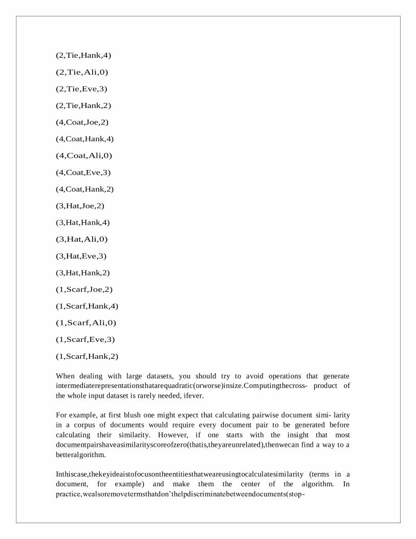
(2,Tie,Hank,4)

(2,Tie,Ali,0)

(2,Tie,Eve,3)

(2,Tie,Hank,2)

(4,Coat,Joe,2)

(4,Coat,Hank,4)

(4,Coat,Ali,0)

(4,Coat,Eve,3)

(4,Coat,Hank,2)

(3,Hat,Joe,2)

(3,Hat,Hank,4)

(3,Hat,Ali,0)

(3,Hat,Eve,3)

(3,Hat,Hank,2)

(1,Scarf,Joe,2)

(1,Scarf,Hank,4)

(1,Scarf,Ali,0)

(1,Scarf,Eve,3)

(1,Scarf,Hank,2)

When dealing with large datasets, you should try to avoid operations that generate

intermediaterepresentationsthatarequadratic(orworse)insize.Computingthecross- product of

the whole input dataset is rarely needed, ifever.

For example, at first blush one might expect that calculating pairwise document similarity

in a corpus of documents would require every document pair to be generated before

calculating their similarity. However, if one starts with the insight that most

documentpairshaveasimilarityscoreofzero(thatis,theyareunrelated),thenwecan find a way to a

betteralgorithm.

Inthiscase,thekeyideaistofocusontheentitiesthatweareusingtocalculatesimilarity (terms in a

document, for example) and make them the center of the algorithm. In

practice,wealsoremovetermsthatdon’thelpdiscriminatebetweendocuments(stop-

words),andthisreducestheproblemspacestillfurther.Usingthistechniquetoanalyze

asetofroughlyonemillion(106)documentsgeneratesintheorderofonebillion

(109)intermediatepairs,9 ratherthantheonetrillion(1012)producedbythenaive

approach(generatingthecross-productoftheinput)ortheapproachwithnostopword removal.

GROUP

AlthoughCOGROUPgroupsthedataintwoormorerelations,theGROUPstatement groups the

data in a single relation. GROUP supports grouping by more than equality of keys: you can

use an expression or user-defined function as the group key. For example, consider the

following relationA:

grunt>DUMP A; (Joe,cherry) (Ali,apple) (Joe,banana) (Eve,apple)

Let’s group by the number of characters in the second field:

grunt>B = GROUP A BY SIZE($1);

grunt>DUMP B;

(5,{(Ali,apple),(Eve,apple)})

(6,{(Joe,cherry),(Joe,banana)})

GROUPcreatesarelationwhosefirstfieldisthegroupingfield,whichisgiventhealias

group.Thesecondfieldisabagcontainingthegroupedfieldswiththesameschemaas the original

relation (in this case,A).

There are also two special grouping operations: ALL and ANY. ALL groups all the tuples in

a relation in a single group, as if the GROUP function was a constant:

grunt>C = GROUP A ALL;

grunt>DUMP C;

(all,{(Joe,cherry),(Ali,apple),(Joe,banana),(Eve,apple)})

Note that there is no BY in this form of the GROUP statement. The ALL grouping is

commonly used to count the number of tuples in a relation.

The ANY keyword is used to group the tuples in a relation randomly, which can be useful for

sampling.

Sorting Data

Relations are unordered in Pig. Consider a relation A:

grunt>DUMP A;

(2,3)

(1,2)

(2,4)

There is no guarantee which order the rows will be processed in. In particular, when

retrieving the contents of A using DUMP or STORE, the rows may be written in any order.

If you want to impose an order on the output, you can use the ORDER operator to sort a

relation by one or more fields. The default sort order compares fields of the same type using

the natural ordering, and different types are given an arbitrary, but deterministic, ordering (a

tuple is always “less than” a bag, for example).

The following example sorts A by the first field in ascending order and by the second field in

descending order:

grunt>B = ORDER A BY $0, $1 DESC;

grunt>DUMP B;

(1,2)

(2,4)

(2,3)

Any further processing on a sorted relation is not guaranteed to retain its order. For example:

grunt>C = FOREACH B GENERATE *;

Even though relation C has the same contents as relation B, its tuples may be emitted

inanyorderbyaDUMPoraSTORE.Itisforthisreasonthatitisusualtoperformthe ORDER

operation just before retrieving theoutput.

The LIMIT statement is useful for limiting the number of results, as a quick and dirty

waytogetasampleofarelation;prototyping(theILLUSTRATEcommand)shouldbe

preferredforgeneratingmorerepresentativesamplesofthedata.Itcanbeusedimme- diately after

the ORDER statement to retrieve the first n tuples. Usually, LIMIT will select any n tuples

from a relation, but when used immediately after an ORDERstate- ment, the order is retained

(in an exception to the rule that processing a relation does not retain itsorder):

grunt>D = LIMIT B 2;

grunt>DUMP D;

(1,2)

(2,4)

If the limit is greater than the number of tuples in the relation, all tuples are returned (so

LIMIT has no effect).

Using LIMIT can improve the performance of a query because Pig tries to apply the limit as

early as possible in the processing pipeline, to minimize the amount of data that needs to be

processed. For this reason, you should always use LIMIT if you are not interested in the

entireoutput.

Combining and Splitting Data

Sometimesyouhaveseveralrelationsthatyouwouldliketocombineintoone.Forthis, the UNION

statement is used. Forexample:

grunt>DUMP A;

(2,3)

(1,2)

(2,4)

grunt>DUMP B;

(z,x,8)

(w,y,1)

grunt>C = UNION A, B;

grunt>DUMP C;

(2,3)

(1,2)

(2,4)

(z,x,8)

(w,y,1)

C is the union of relations A and B, and since relations are unordered, the order of the tuples

in C is undefined. Also, it’s possible to form the union of two relations with

differentschemasorwithdifferentnumbersoffields,aswehavedonehere.Pigattempts

tomergetheschemasfromtherelationsthatUNIONisoperatingon.Inthiscase,they are

incompatible, so C has noschema:

grunt>DESCRIBE A; A: {f0: int,f1: int} grunt>DESCRIBEB;

B: {f0: chararray,f1: chararray,f2: int} grunt>DESCRIBEC;

Schema for C unknown.

If the output relation has no schema, your script needs to be able to handle tuples that vary in

the number of fields and/or types.

TheSPLIToperatoristheoppositeofUNION;itpartitionsarelationintotwoormore relations..

Pig in Practice

There are some practical techniques that are worth knowing about when you are developing

and running Pig programs. This section covers some of them.

Parallelism

When running in MapReduce mode it’s important that the degree of parallelism

matchesthesizeofthedataset.Bydefault,Pigwillsetsthenumberofreducersby

lookingatthesizeoftheinput,andusingonereducerper1GBofinput,uptoamax-

imumof999reducers.Youcanoverridetheseparametersbysettingpig.exec.reducers.bytes.pe

r.reducer (the default is 1000000000 bytes) and pig.exec.reducers.max (default999).

Toexplictlysetthenumberofreducersyouwantforeachjob,youcanuseaPARALLEL clause for

operators that run in the reduce phase. These include all the grouping and joining operators

(GROUP, COGROUP, JOIN, CROSS), as well as DISTINCT and ORDER. The following

line sets the number of reducers to 30 for theGROUP:

grouped_records = GROUP records BY year PARALLEL 30;

Alternatively, you can set the default_parallel option, and it will take effect for all

subsequent jobs:

grunt>set default_parallel 30

A good setting for the number of reduce tasks is slightly fewer than the number of reduce

slots in the cluster.

Thenumberofmaptasksissetbythesizeoftheinput(withonemapperHDFSblock) and is not

affected by the PARALLELclause.

Parameter Substitution

IfyouhaveaPigscriptthatyourunonaregularbasis,thenit’squitecommontowant

tobeabletorunthesamescriptwithdifferentparameters.Forexample,ascriptthat

runsdailymayusethedatetodeterminewhichinputfilesitrunsover.Pigsupports parameter

substitution, where parameters in the script are substituted with values

suppliedatruntime.Parametersaredenotedbyidentifiersprefixedwitha$character;

forexample,$inputand$outputareusedinthefollowingscripttospecifytheinput and

outputpaths:

-- max_temp_param.pig

records = LOAD '$input' AS (year:chararray, temperature:int, quality:int);

filtered_records = FILTER records BY temperature != 9999 AND

(quality == 0 OR quality == 1 OR quality == 4 OR quality == 5 OR quality == 9);

grouped_records = GROUP filtered_records BY year;

max_temp = FOREACH grouped_records GENERATE group,


STORE max_temp into '$output';

ParameterscanbespecifiedwhenlaunchingPig,usingthe-paramoption,oneforeach parameter:

% pig -param input=/user/tom/input/ncdc/micro-tab/sample.txt \

> -param output=/tmp/out\

> ch11/src/main/pig/max_temp_param.pig

YoucanalsoputparametersinafileandpassthemtoPigusingthe-param_fileoption. For example,

we can achieve the same result as the previous command by placing the parameter

definitions in afile:

# Input file

input=/user/tom/input/ncdc/micro-tab/sample.txt # Outputfile

output=/tmp/out

The pig invocation then becomes:

% pig -param_file ch11/src/main/pig/max_temp_param.param \

> ch11/src/main/pig/max_temp_param.pig

You can specify multiple parameter files using -param_file repeatedly. You can also use a

combination of -param and -param_file options, and if any parameter is defined in both a

parameter file and on the command line, the last value on the command line takesprecedence.

HIVE

In “Information Platforms and the Rise of the Data Scientist,”1 Jeff Hammerbacher describes

Information Platforms as “the locus of their organization’s efforts to ingest, process, and

generate information,” and how they “serve to accelerate the process of learning from

empirical data.”

OneofthebiggestingredientsintheInformationPlatformbuiltbyJeff’steamatFace- book was

Hive, a framework for data warehousing on top of Hadoop. Hive grewfrom

aneedtomanageandlearnfromthehugevolumesofdatathatFacebookwasproducing

everydayfromitsburgeoningsocialnetwork.Aftertryingafewdifferentsystems,the

teamchoseHadoopforstorageandprocessing,sinceitwascost-effectiveandmettheir

scalabilityneeds.2

Hive was created to make it possible for analysts with strong SQL skills (but meager Java

programming skills) to run queries on the huge volumes of data that Facebook

storedinHDFS.Today,HiveisasuccessfulApacheprojectusedbymanyorganizations as a

general-purpose, scalable data processingplatform.

Of course, SQL isn’t ideal for every big data problem—it’s not a good fit forbuilding

complex machine learning algorithms, for example—but it’s great for many analyses, and it

has the huge advantage of being very well known in the industry. What’smore,

SQListhelinguafrancainbusinessintelligencetools(ODBCisacommonbridge,for example), so

Hive is well placed to integrate with theseproducts.

ThischapterisanintroductiontousingHive.Itassumesthatyouhaveworkingknowl-

edgeofSQLandgeneraldatabasearchitecture;aswegothroughHive’sfeatures,we’ll often

compare them to the equivalent in a traditionalRDBMS.

Installing Hive

Innormaluse,HiverunsonyourworkstationandconvertsyourSQLqueryintoaseries

ofMapReducejobsforexecutiononaHadoopcluster.Hiveorganizesdataintotables, which

provide a means for attaching structure to data stored in HDFS. Metadata— such as table

schemas—is stored in a database called themetastore.

When starting out with Hive, it is convenient to run the metastore on your local machine. In

this configuration, which is the default, the Hive table definitions that you create will be local

to your machine, so you can’t share them with other users. We’ll see how to configure a

shared remote metastore, which is the norm in production environments.

Installation of Hive is straightforward. Java 6 is a prerequisite; and on Windows, you will

need Cygwin, too. You also need to have the same version of Hadoop installed

locallythatyourclusterisrunning.3Ofcourse,youmaychoosetorunHadooplocally,

eitherinstandaloneorpseudo-distributedmode,whilegettingstartedwithHive.These options are

all covered in AppendixA.

Download a release at http://hive.apache.org/releases.html, and unpack the tarball in a

suitable place on your workstation:

% tar xzf hive-x.y.z-dev.tar.gz

It’s handy to put Hive on your path to make it easy to launch:

% export HIVE_INSTALL=/home/tom/hive-x.y.z-dev

% export PATH=$PATH:$HIVE_INSTALL/bin

NowtypehivetolaunchtheHiveshell:

% hive

hive>

Running Hive

Inthissection,welookatsomemorepracticalaspectsofrunningHive,includinghow to set up Hive

to run against a Hadoop cluster and a shared metastore. In doing so, we’ll see Hive’s

architecture in somedetail.

Configuring Hive

Hive is configured using an XML configuration file like Hadoop’s. The file is called hive-

site.xmlandislocatedinHive’sconfdirectory.Thisfileiswhereyoucansetprop- erties that you

want to set every time you run Hive. The same directory containshive-

default.xml,whichdocumentsthepropertiesthatHiveexposesandtheirdefaultvalues.

YoucanoverridetheconfigurationdirectorythatHivelooksforinhive-site.xmlby passing the -

-config option to the hivecommand:

% hive --config /Users/tom/dev/hive-conf

Note that this option specifies the containing directory, not hive-site.xml itself. It can be

useful if you have multiple site files—for different clusters, say—that you switch between on

a regular basis. Alternatively, you can set the HIVE_CONF_DIRenvironment variable to the

configuration directory, for the sameeffect.

http://hive.apache.org/releases.html

Thehive-site.xmlisanaturalplacetoputtheclusterconnectiondetails:youcanspecify the

filesystem and jobtracker using the usual Hadoop properties, fs.default.name and

mapred.job.tracker (see Appendix Afor more details on configuring Hadoop). If not set, they

default to the local filesystem and the local (in-process) job runner—justlike

theydoinHadoop—whichisveryhandywhentryingoutHiveonsmalltrialdatasets. Metastore

configuration settings are commonly found in hive-site.xml,too.

Hive also permits you to set properties on a per-session basis, by passing the

-hiveconfoptiontothehivecommand.Forexample,thefollowingcommandsetsthe

cluster(toapseudo-distributedcluster)forthedurationofthesession:

% hive -hiveconf fs.default.name=localhost -

hiveconfmapred.job.tracker=localhost:8021

IfyouplantohavemorethanoneHiveusersharingaHadoopcluster, then you need to make the

directories that Hive uses writable by all

users.Thefollowingcommandswillcreatethedirectoriesandsettheir permissionsappropriately:

% hadoopfs -mkdir/tmp

% hadoopfs -chmoda+w /tmp

% hadoop fs -mkdir /user/hive/warehouse

% hadoopfs -chmoda+w /user/hive/warehouse

Ifallusersareinthesamegroup,thenpermissionsg+waresufficienton the warehousedirectory.

You can change settings from within a session, too, using the SET command. This is

usefulforchangingHiveorMapReducejobsettingsforaparticularquery.Forexample,

thefollowingcommandensuresbucketsarepopulatedaccordingtothetabledefinition.

hive>SET hive.enforce.bucketing=true;

To see the current value of any property, use SET with just the property name:

hive>SET hive.enforce.bucketing;

hive.enforce.bucketing=true

Byitself,SETwilllistalltheproperties(andtheirvalues)setbyHive.Notethatthelist

willnotincludeHadoopdefaults,unlesstheyhavebeenexplicitlyoverriddeninoneof the ways

covered in this section. Use SET -v to list all the properties in the system, including

Hadoopdefaults.

Thereisaprecedencehierarchytosettingproperties.Inthefollowinglist,lowernum- bers take

precedence over highernumbers:

1. The Hive SETcommand

2. The command line -hiveconfoption

3. hive-site.xml

4. hive-default.xml

5. hadoop-site.xml (or, equivalently, core-site.xml, hdfs-site.xml, and mapred- site.xml)

6. hadoop-default.xml (or, equivalently, core-default.xml, hdfs-default.xml,and

mapred-default.xml)

DATA TYPES

Hive supports both primitive and complex data types. Primitives include numeric, boolean,

string, and timestamp types. The complex data types include arrays, maps, and structs.. Note

that the literals shown are those used from within HiveQL; they are not the serialized form

used in the table’s storage format.

Primitive types

Hive’s primitive types correspond roughly to Java’s, although some names are influ- enced

by MySQL’s type names (some of which, in turn, overlap with SQL-92).There

arefoursignedintegraltypes:TINYINT,SMALLINT,INT,andBIGINT,whichareequivalent

toJava’sbyte,short,int,andlongprimitivetypes,respectively;theyare1 -byte,2-byte, 4-byte, and 8-

byte signedintegers.

Hive’sfloating-pointtypes,FLOATandDOUBLE,correspondtoJava’sfloatanddouble,

whichare32-bitand64-bitfloatingpointnumbers.Unlikesomedatabases,thereisno

optiontocontrolthenumberofsignificantdigitsordecimalplacesstoredforfloating

pointvalues.

Hive supports a BOOLEAN type for storing true and false values.

There is a single Hive data type for storing text, STRING, which is a variable -length

character string. Hive’s STRING type is like VARCHAR in other databases, although there

is no declaration of the maximum number of characters to store with STRING. (The

theoreticalmaximumsizeSTRINGthatmaybestoredis2GB,althoughinpracticeitmay be

inefficient to materialize such large values. Sqoop has large object support.

The BINARY data type is for storing variable-length binary data.

The TIMESTAMP data type stores timestamps with nanosecond precision. Hive comes with

UDFs for converting between Hive timestamps, Unix timestamps (seconds since the Unix

epoch), and strings, which makes most common date operations tractable. TIMESTAMP

does not encapsulate a timezone, however the to_utc_timestamp andfrom_utc_timestamp

functions make it possible to do timezone conversions.

Conversions

Primitivetypesformahierarchy,whichdictatestheimplicittypeconversionsthatHive will

perform. For example, a TINYINT will be converted to an INT, if an expressionex-

pects an INT; however, the reverse conversion will not occur and Hive will return an error

unless the CAST operator is used.

Theimplicitconversionrulescanbesummarizedasfollows.Anyintegralnumerictype can be

implicitly converted to a wider type. All the integral numeric types, FLOAT,and (perhaps

surprisingly) STRING can be implicitly converted to DOUBLE. TINYINT, SMALLINT,

and INT can all be converted to FLOAT. BOOLEAN types cannot be converted to any

othertype.

You can perform explicit type conversion using CAST. For example, CAST('1' AS INT) will

convert the string '1' to the integer value 1. If the cast fails—as it does in CAST('X' AS

INT), for example—then the expression returns NULL.

Complex types

Hive has three complex types: ARRAY, MAP, and STRUCT. ARRAY and MAP are like

their namesakes in Java, while a STRUCT is a record type which encapsulates a set of named

fields. Complex types permit an arbitrary level of nesting. Complex type declarations must

specify the type of the fields in the collection, using an angled bracket notation, as illustrated

in this table definition which has three columns, one for each complex type:

CREATE TABLE complex ( col1 ARRAY<INT>,

col2 MAP<STRING, INT>,

col3 STRUCT<a:STRING, b:INT, c:DOUBLE>

);

IfweloadthetablewithonerowofdataforARRAY,MAP,andSTRUCTshowninthe“Literal

examples”then the following query demonstrates the field accessor operators for eachtype:

hive>SELECT col1[0], col2['b'], col3.c FROM complex;

OPERATORS AND FUNCTIONS

The usual set of SQL operators is provided by Hive: relational operators (such as x = 'a' for

testing equality, x IS NULL for testing nullity, x LIKE 'a%' for pattern matching),

arithmetic operators (such as x + 1 for addition), and logical operators (such as x OR y for

logical OR). The operators match those in MySQL, which deviates from SQL-92 since || is

logical OR, not string concatenation. Use the concat function for the latter in both MySQL

and Hive.

Hive comes with a large number of built-in functions—too many to listhere—divided into

categories including mathematical and statistical functions, string functions, date functions

(for operating on string representations of dates), conditional functions,aggregate functions,

and functions for working with XML (using the xpath function)and JSON.

YoucanretrievealistoffunctionsfromtheHiveshellbytypingSHOWFUNCTIONS.6To get brief

usage instructions for a particular function, use the DESCRIBEcommand:

hive>DESCRIBE FUNCTION length;

length(str) - Returns the length of str

USER-DEFINED FUNCTIONS

Sometimes the query you want to write can’t be expressed easily (or at all) using the built -in

functions that Hive provides. By writing a user-defined function (UDF), Hive makes it easy

to plug in your own processing code and invoke it from a Hive query.

UDFs have to be written in Java, the language that Hive itself is written in. For other

languages,considerusingaSELECTTRANSFORMquery,whichallowsyoutostreamdata

through a user-defined script.

TherearethreetypesofUDFinHive:(regular)UDFs,UDAFs(user-definedaggregate functions),

and UDTFs (user-defined table-generating functions). They differ in the numbers of rows

that they accept as input and produce asoutput:

• A UDF operates on a single row and produces a single row as its output. Most functions,

such as mathematical functions and string functions, are of thistype.

• AUDAFworksonmultipleinputrowsandcreatesasingleoutputrow.Aggregate functions

include such functions as COUNT andMAX.

• AUDTFoperatesonasinglerowandproducesmultiplerows—atable—asoutput.

Table-generating functions are less well known than the other two types, so let’s look

atanexample.Consideratablewithasinglecolumn,x,whichcontainsarraysofstrings. It’s

instructive to take a slight detour to see how the table is defined andpopulated:

CREATE TABLE arrays (x ARRAY<STRING>) ROW FORMAT DELIMITED

FIELDS TERMINATED BY '\001'

COLLECTION ITEMS TERMINATED BY '\002';

Notice that the ROW FORMAT clause specifies that the entries in the array are delimited by

Control-B characters. The example file that we are going to load has the following contents,

where ^B is a representation of the Control-B character to make it suitable for printing:

a^Bbc^Bd^Be

After running a LOAD DATA command, the following query confirms that the data was

loaded correctly:

hive >SELECT * FROM arrays;

["a","b"] ["c","d","e"]

Next, we can use the explode UDTF to transform this table. This function emits a row for

each entry in the array, so in this case the type of the output column y is STRING. The result

is that the table is flattened into five rows:

hive >SELECT explode(x) AS y FROM arrays;

a b c d e

SELECT statements using UDTFs have some restrictions (such as not being able to retrieve

additional column expressions), which make them less useful in practice. For this reason,

Hive supports LATERAL VIEW queries, which are more powerful.

big data and business analytics - iare

Documents