bifurcations in stochastic dynamical systems with simple
TRANSCRIPT

Stochastic Processes and their Applications 31 (1989) 71-88
North-Holland
71
BIFURCATIONS IN STOCHASTIC DYNAMICAL
SYSTEMS WITH SIMPLE SINGULARITIES
Stanislaw JANECZKO*
Department of Mathematics, Monash University, Clayton, Victoria 3168, Australia
Eligiusz WAJNRYB
Institute of Theoretical Physics, Warsaw University, Hoia 69, 00-691 Warsaw, Poland
Received 16 September 1987
Revised 13 July 1988
The generalized Langevin stochastic dynamical system is introduced and the stationary probability
density for its solution is investigated. The stochastic field is assumed to be singular with a simple
singularity, and noise in the control parameters is modelled as dychotomous Markov noises. A
classification of bifurcation diagrams for the stationary density probability is obtained. Two
examples encountered from physics, the dye laser model and the Verhulst model, are investigated.
stochastic process * dynamical system * singularity * bifurcation diagram
1. Introduction
The main interest of recent bifurcation theory (cf. [2,6]) has been to determine
bifurcation diagrams and the corresponding structural changes in the system under
consideration. For the generic, finitely-determined models of singularity theory (cf.
[4, 141) these bifurcation sets (also called catastrophe sets [15]) are well known and
their relevance for the understanding of various physical, chemical and biological
systems has been exhaustively proved in a number of recent publications (see e.g.
[15,6, 14, 171). It appears, however, that in realistic laser systems (cf. [5]) critical
region phenomena (cf. [S]) or various open or semiopen chemical or thermodynami-
cal systems, random internal fluctuations play an important role. It is therefore
necessary to include in the model the stochastic component of the noise. Stochasticity
of some control parameters of the standard dynamical models tends to completely
change bifurcation diagrams. Their use is an important physical branch of the theory
of stochastic processes (cf. [7, 161). Abstracting from the concrete models we see
that the structure of these stochastic bifurcation sets is interesting even for the theory
itself. In this paper we investigate the bifurcation sets for a wide class of stochastic
dynamical systems, coming from standard singularity theory with Markovian
dychotomous noise. The paper deals only with l-dimensional stochastic dynamical
systems. We do not pretend to give a complete description of such systems but
merely to investigate some interesting examples and the universal problems suggested
by them.
* On leave from Institute of Mathematics, Technical University of Warsaw, PI. JednoSci Robotniczej 1, 00-661 Warsaw, Poland.
0304-4149/89/$3.50 @ 1989, Elsevier Science Publishers B.V. (North-Holland)

12 S. Janeczko, E. Wajnryb / Stochastic dynamical systems
In the first section we give some necessary preliminaries concerning stochastic
dynamical systems and propose a geometrical method to investigate their probability
densities. Section 3 is devoted to a presentation of various physical systems with
stochastic noise, as for example the dye laser system with pre-Gaussian pump
fluctuations. This problem can be seen as the main motivation for our study. In
Section 4 we develop a theory for stable dynamical systems with a stochastic control
space and prove some generic properties. We show that the equations for stationary
probability densities reduce to equations with so-called regular singular points. The
analysis of bifurcation diagrams for stable dynamical systems is provided in Section
5, where the appropriate “topological type function” is introduced. The fold model
and the cusp model with dychotomous one dimensional noise are investigated and
the corresponding bifurcation diagrams are obtained.
2. Stochastic dynamical systems driven by the dychotomous Markov noise
Many systems of practical interest can be described by a single relevant variable.
This variable as a function of time is governed by a first-order differential equation
of motion which additionally depends on external control parameters (see e.g. [14]).
If it is assumed that there exist a fluctuating control parameter (external noise [16])
the deterministic equation of motion (usually) transforms into a stochastic one of
the form
(1)
where u(t) is the external noise, f(x) is the deterministic vector field and g(x)
represents a linear coupling of the fluctuating parameter u(t) with the coordinate
x. Equation (1) is the most common case in a large number of real situations; it is
called a Langevin equation (cf. [ 12,161) Assuming that u(t) is Gaussian white noise
(cf. [7]), i.e.
(u(t)) = 0, (u(l)u(l'))=2r6(l-t'),
we see that the stochastic process x(t) is Markovian and the probability density
P(x, t) satisfies the differential Fokker-Planck equation (see [ 161)
If u(t) is not white noise the process x(t) is not a Markov process.
In this paper we consider (1) when the stochastic process u(t), which is possibly
multidimensional, is a dychotomous Markov noise. In this case u(t) takes two
possible values, a and --a, a > 0 with transition rates, from a to -a and vice versa,
equal to y/2. Let P,(t) =d”FProbability {u(t) = *a}. The Master equation for P* (1)

S. Janeczko, E. Wajnryb / Stochastic dynamical systems 73
(see [l]) then reads as
(4)
If P*(O) = i then u(t) is a stationary process with the correlation function
(u(t)u(t’))=a’e . --y/f-C (5)
For the detailed information on this type of processes we refer the reader to [ 16, 121.
Instead of the Langevin equation (1) for X(I) we can write the Liouville equation
satisfied by the corresponding density 4,
4(Y, r) = G(Y-x(r)), (6)
namely
where x(t) is the solution to equation (1) with initial condition x,, and the definite
realisation of the stochastic trajectory u(t). In fact we are interested in the probability
density P( y, t), which is defined as
P(Y, t) = (4(Y, t)), (8)
where (.) defines an average over all realisations of u(t) according to equation (4).
Combining the equations (4) and (7) we obtain two Master equations for the
probability densities P&(x, t), namely
; P+(x, I)=-;f(x)P+cx, r)a+)P+b, t)-;YP+(x, t)+;YP-(4 I), (9)
; P-(x, t) = -S./(x) P-(x, t) + a$(x)P_(x, t)+Z P+(x, t) -; P-(x, t). (10)
Here P&(x, t) dx denotes the joint infinitesimal probability for x at time t and
u(t) = ia. Using the new functions
P(x, t) = P+(x, t)+ P-(x, t), ax, t) = P+(x, t) - P-(x, f), (11)
where P(x, t) is probability density of the variable x, independent of external noise
u(t), we can rewrite equations (9) and (10) in the form
; P(x, t) = -$f(xMx, t) -u; g(x)Q(x, t),
; ax, f) = -~f(x)Ob, f) -7; dx)P(x, t) - Tax, t).
(12)
(13)
Now we are interested in the stationary solutions; PS,(x), C&,(x), of the above
equations. By (12) we have
f(x)p,,(x) + ag(x)%(x) =j = const(x). (14)

74 S. Janeczko, E. Wajnryb / Stochastic dynamical systems
Let us put j equal to zero. This assumption does not restrict the generality of our
approach. We insert Q.%,, derived from (14), to (13) and obtain the following
differential equation for the stationary pF, :
a f’(x) - a2g2(x)
G ( g(x) Pf,(X)
> = -g P,,(x).
This equation has the general solution (cf. [11])
x
dx’ f (x’)
a2g2(x’) -f 2(x’) .
Additionally, we have
Qs,(x) = -$9,,(x), (17)
1 P:,(x) = -~
Zag(x) F_(x)P,,(x),
P,(x)=- * ___ F-(x)P,,(x), zag(x)
(18)
(19)
(15)
(16)
where F,(x) =f(x) * ag(x).
Remark 2.1. From physical arguments it is concluded that P;’ and P, are not
negative functions. From equations (18), (19) we see that we can satisfy this
requirement if and only if F+ and F_ have opposite signs. This observation is also
very helpful in the geometrical interpretation of stable physical domains defining
the stationary probability density involved in equation (15). This interpretation was
introduced in [5] and describes the stable physical domains as defined by the
stochastic vector fields F+, F- in competition.
3. Applications to the open systems in a fluctuating environment
To discuss the ideas for various applications we begin by noting that the random
force which occurs in a Langevin equation (1) can have quite different origins. In
an ordinary microscopic derivation of a Langevin equation (see e.g. [ 161) the random
term u( t)g( t) is associated with the “thermal” or “internal” noise - thermal fluctu-
ations, especially near a critical point (cf. [8,7]).
A different and more common interpretation of the random term of a Langevin
equation is necessary, however when this is thought to model what we call an
“external noise” situation. This type of fluctuation can be due to a varying environ-
ment or can be the result of an externally applied random force. The mathematical
modelling of these fluctuations is made by formulating the appropriate deterministic
equation in the absence of external fluctuations. One then lets the external parameter,

S. Janeczko, E. Wajnryb / Stochastic dynamical systems 75
which undergoes fluctuations, be a stochastic variable. The noise term of the
stochastic differential equation obtained in this way, usually has a multiplicative
character, i.e. it depends on the instantaneous value of the variables of the system.
We can take the external noise as an external stochastic field which drives the system
(cf. [ 161).
Dynamical equations of motion with random noise have been first used in the
theory of Brownian motion. The best known examples of such Langevin equations
are
where f(x) = 0, g(x) = 1 (as in equation (1)) and x denotes the position of the
particle. Another example is
$o=-AViU(f) (21)
wheref( u) = -Au, g(v) = 1, u is the velocity of the particle and in both these examples
u(t) is a random noise due to to the external random collisions. If u(t) is a Gaussian
white noise (see Section 2), then equation (20) leads through equation (3) to the
well known Wiener-Levy process described by the diffusion equation for the proba-
bility density P(x, t):
; P(x, t) = r-$ P(x, t).
Analogously, insertingf and g from example (21) into equation (3) (see Section 2)
we obtain the following equation for the density probability P(v, t):
which describes the evolution of the Ornstein-Uhlenbeck process.
Another use of stochastic dynamical systems has been made in the modelling of
a more realistic laser with pump fluctuations (see [5,9, IO]). Again the random
process composed of two random telegraph processes appears to be useful in
approximation of the Ornstein-Uhlenbeck process representing the chaotic fluctu-
ations in the system. Let us consider the dye-laser equation (cf. [5,9])
5x=(* -x)x+xz(t),
where z(t) = u,(t) + u2( t) is the two telegraph additive noise. The corresponding
equation for the stationary probability density,
(23)

76
where
S. Janeczko, E. Wajnryb / Stochastic dynamical systems
g(x) = 4 f(x) = Ax -x2, Y(X) = I “& g ’
reduces to the standard Fuchs type equation of second order. The local behaviour
of P,, at singular points was investigated in [5]. The bifurcating family of supports
for this model is illustrated in Fig. 1.
As an example of a Langevin equation used in quantum optics let us take the
propagation of a pulse in a nonlinear random medium. The propagation equation
in the z direction of a wave evolution has the form ([16])
g f(z)= &I+ u(z)
1-t LJ(z) f(z). (24)
Fig. 1

S. Janeczko, E. Wajnryb / Stochastic dynamical systems 77
In this equation, u(z) describes the random properties of the medium. Another
example of the Langevin equation with external noise in quantum optics can be
given by the rate equations for multiphoton processes. The changes of atomic
population due to one or two photon ionisation in the presence of a fluctuating
laser light are given by the equations (cf. [7])
(25)
where u(t) is the external field amplitude which fluctuates according to external
conditions.
In all these examples u(t) may be an arbitrary noise process. The most trivial
case is of white noise and such systems are described by the Fokker-Planck equations,
except for (25) where the noise enters nonlinearly. In the rest of the paper we are
interested in a more realistic situation with nonwhite external noise represented by
random telegraphs, possibly entering nonlinearly.
4. Stable dynamical systems in the stochastic control space
Let us consider a general stochastic dynamical system with one internal variable
(cf. r 121),
i=-grad, V(x, ul(t) ,..., u,(t))=F(x, ul(t) ,..., u,,(t)), (26)
where ur( t), . . . , u,(t) are independent stochastic processes and F is a smooth
function. We allow (26) to be a general nonlinear system. Because of its simplicity
and extensive use in applications (see Section 2 and 3) we restrict our considerations
to the Markovian dychotomous noises ul(t), . . . , u,(t). In this case we have the
following result.
Proposition 4.1. Let
i=F(x; i&u,(t) )...) u,(t)), U=(U ,,..., UJCRk (27)
be a dynamical stochastic system parametrized by deterministic control variables (ii,) f
and Markovian dychotomous noises (u,) ;. Then there exist smooth functions
(gi(x, u))Y, (gi,i,(x3 u))tz-i2, . . . 9 (gl,,...,l,,(x9 u))Y,>.,.>i,, 9
such that (27) has the form
a=f(x, u)+ i gi(X, 22)Ui(t)+ i: gi,i,(X, ti)Ui,(t)U,2(t)+e ” i=l i,>iz
+ 5 gt,...i,,Cx, u)"i,(r) ’ ’ . ui,,(t).
i,>...>i,,
(28)

78 S. Janeczko, E. Wajnryb / Stochastic dynamical systems
In other words the general stochastic system (27) is equal to one with stochastic variables
entering linearly, i.e.
x=f(x~ u)+ i gitx, u)wt(t), (29) i=l
where wi( t) are, not necessarily independent, stochastic variables representing also
dychotomous processes as multiplicatively composed initial telegraphs (i.e. wi( t) is a
product of some number of independent telegraph noises so is also dychotomous).
Proof. For the one telegraph noise, say u(t) (realized by an integer valued stochastic
process n(t, to), i.e. u(t) = a(-l)““‘“‘, a > 0, cf. [l]). For its two values +a, -a we
have
Thus the
F(x, ii, +a) =:(F(x, U, a)+F(x, ii, -a))+ T(F( x, 6, a) - F(x, 6, -a)),
F(x, U, -a) = $(F(x, U, a) + F(x, ii, -a)) + $$(F( x, ii, a) - F(x, 6, -a)).
stochastic dependence of F(x, 6, u(t)) can be written in the form
F(x, ii, u(t)) =+(F(x, ii, a)+F(x, ii, -a))
+$(F(x,ti, a)-F(x, ii, -a)).
Now we can treat (*) as a first step in the induction process with respect to the
number of telegraphs in E Repeating decomposition (*) with respect to second,
third, . . . , nth telegraphs successively we directly obtain the desired result (28).
Remark 4.2. For the deterministic dynamical system of type (27) its stationary
surface (the set of zeros of the corresponding field F) gives basic information about
the slow dynamics appearing in various dynamical models of physical systems (see
[15,17]). The general nonlinear system of type (27) can be very complicated with
regard to its stationary properties. However, when we remove some very small class
of “pathological” (unstable) systems, the theory of singularities (see [4, 141) provides
complete information about the local stationary properties of typical nonlinear
systems.
Now we recall some necessary basic facts from standard singularity theory. Let
f = -grad, V(x, u) be a dynamical system with smooth potential V: [w x [Wk + [w. We
say that this system is stable if at each point (x0, uO) E [w x Rk the following holds
(cf. [14, 171): the quotient ring mC,,,/J( V) is generated by {aV(x, t)/aUi}f=, as an
&,,, module (cf. [4]). Here by mCX,,,c ,$CX,Uj, (&,,,) we denote the maximal ideal of
the ring [CX,Uj of germs at (x,, uO), ((u,) -resp.) of smooth functions and by J(V)
we denote the corresponding ideal generated by JV(x, u)/ax. It appears that for

S. Janeczko, E. Wajnrvb / Stochastic dynamical systems 79
structurally stable systems (by the Malgrange Preparation Theorem [4]), in a neigh-
bourhood of each point (x,, uO) the system is equivalent, in its stationary dynamics,
to one given in the form (cf. Proposition 4.1)
x = -grad, V,+(X, U) =f(x) + i Uigi(X), /_L s k, (30) i=*
where we assume (x0, u,,) = (0,O) and the gi(x) are smooth functions generating the
space 5&J(f) (cf. [4,151). Comparing the form of the system given by the above potentials to the stochastic
one (28) with telegraphically fluctuating control parameters we are also encouraged
to restrict ourselves to dynamical systems with stable potentials (30). It also suggests
that we should consider additional stochastic noises entering additively in the
deterministic parameters (Ui).
Thus, in what follows, we assume our stochastic dynamical system to be recon-
structed from a stable (30) deterministic one by switching on the respective telegraphs
associated with each control parameter, the values of which are treated as the
fluctuating centres of external forces. Thus we have
x=-grad, V,(x, ii)+ f ui(t)hi(x) ( >
, (31) i=l
where the functions hi(x) are determined by the stable deterministic potential V,
at the neighbourhood of each point (x, u).
Let x = F(x, ii, u(t)) be a stochastic system
direct product of independent dychotomous
equations for the respective probabilities are
p(+L(p”‘_p$)) 2r,
>
PCy)(t) =-!- (p(i) _ pp))
27;+ ’ Ti > 0,
where u(t)=(u,(t),...,u,(t)) is a
noises. The corresponding Master
(32)
(33)
and the amplitudes ai > 0, i.e. (ui( t)ui( t’)) = af e~“~“i’T~.
The stochastic solution of (26) is characterized by its joint probability density,
sayP,(x,t),I=(i,,.. . , i,,), ij = f , which is governed by the joint probability Master
equation (cf. [16, 111)
; p,(x, t) = -; F(x, A,)P,(x, t) -iI{, ; (PI - pt,)k f),
where, J=(i ,,..., -4 ,..., i,,) and A, is a value of u(t) corresponding to I, i.e.
A, = (i,a,, . . . , &a,).
Let us order the set of indices I (say: (+, +, . . .), (-, +, . . .), (+, -, . . .), (-, -, . . .)
etc.). Then we can write the system F(x, A,)P,(x, t) as a column vector, say 2 Thus

80 S. Janeczko, E. Wajnryb / Stochastic dynamical systems
for the modified stationary density probability P(x), on the basis of (34), we have
the equation
2 P(x) = B(x)ji(x), (35)
where B(x) = TF -(x), F(x) is a matrix function with F(x, A,)-entries on the
diagonal, ( F-‘(x))~~ = 6,k/ F(x, A,) and T = ( TrJ) is a constant matrix defined by
T,,=f; ‘&I,-: ,g,i &J. j=* 7j (. >
(36)
Taking into account equation (28) and the form of matrix B(x) with rational entries
we have the following result.
Proposition 4.3. For the generic stochastic system (27) the corresponding system of
equations for the joint stationary probability, considered in the complex domain, is a
system of equations with regular singularities (cf [ 131).
Remark 4.4. On the basis of Proposition 4.3 we can use the standard theory of
differential equations (see [13,3]) and analyse the behaviour of a physically accep-
table solution P(x) in the neighbourhood of singular points, for the generic stochastic
systems without parameters. However in stochastically controlled systems, even
generic ones, the confluencies of singularities appear and the complete analysis of
any solution is much more complicated. In order to analyse the controlled systems
we restrict ourselves to ones with one dychotomous noise, i.e. n = 1 in formula (27).
We recall that p is a number of control parameters nontrivially entering into F,
while k denotes the dimension of control space - this is a standard setting of
singularity theory [14]. More general analysis and the connection between the
solutions of (34) and monodromy theorems in singularity theory (see [3]) we leave
to a forthcoming paper.
In the case of one dychotomous noise the stochastic dynamics is governed by
two potentials (see equation (26)), V*( x, U) = V(x, U, +a). Thus, on the basis of
Remark 2.1, we can completely characterize the topological structure of the support
of the stationary probability density (cf. [5,9]).
Let x0 be a finite critical point of one of the potentials V,. Let 2i denote the
order of this point if it is a minimum, and by (2i+ I), we distinguish the two kinds
of injection point of order (2i + 1) (i.e. nondecreasing “+” or nonincreasing “-“).
Proposition 4.5. The following configurations of potentials V+, V- (with at most one
critical point x0, as illustrated in Fig. 2) form, at x0, the support boundary point, s.b.p.
for short:
(a) Right s.6.p. If V+ and V- (or in opposite order) are of order 2i or (2i+ 1)) and
(2 . 0+ l), respectively. We denote these configurations by R2’, R”+‘.
(b) Left s.b.p. Zf V+ and V- (or in opposite order) are of order 2i or (2i+ l)+ and
(2 . 0+ l)_ respectively. We denote these configurations by L2’, L”+‘.

81 S. Janeczko, E. Wajnryb / Stochastic dynamical systems
These four configurations are illustrated in Fig. 2.
Proof. We can integrate (34) and obtain
Assuming that x0 is a finite critical point of one of the
(d/dx) V-(x,, ii) = -F-(x,, ii) = 0, we obtain by analysing
the neighbourhood of x0,
potentials, say V+, and
the formula (37) that, in
for k3 1
Lb> - 1
Fi”(x,,, U)(x-x0)’ exp
yk! 2(k-l)Fik’(xo, ti)
(x-xp) (38)
and
p,, _ Ix - xOJ y/2r:(%u)- (39)
for k= 1. Verifying the integrabihty (i.e. existence of I:,, P*,(x) dx) of these
formulas we obtain the conclusion of Proposition 4.5.
L2i+l )
LL x
\
\ \ ; \ \ ‘*, ‘1 \ \ \ \ \ \
‘._’
V
I x
‘\ VA
Fig. 2

82 S. Janeczko, E. Wajnryb / Stochastic dynamical systems
Corollary 4.6. For the dychotomous Markov noise, with potentials V+, V- in general
position the only support boundary points which appear have the type R2 or L2 (see
Fig. 2), with the corresponding index of divergence
Y -1 or
Y
2FL(x, zi) 2FI_(x,, U) -1. (40)
5. Stochastic bifurcation sets for elementary catastrophes
In the framework of standard singularity theory one classifies the potential functions
g : R” -+ R with respect to the properties and configurations of their degenerate critical
points. From results on structural stability (cf. [ 151) these investigations are usually
conducted, locally in the neighbourhood of a critical point and using the language
of germs (i.e. the classes of smooth functions identified in some neighbourhood of
the source point of the germ [4]). However to avoid inessential rigour we speak
about functions instead of their germs.
Let g :R”, O+ R be a singularity, g E tCX,, i.e. g has an isolated critical point at
0 E R”. An unfolding of a singularity is a “parametrized family of perturbations”.
These parameters are treated usually as control parameters [ 141. The notion is useful
mainly because, for finite codimension singularities (cf. [17]), there exists a “uni-
versal unfolding” which in a sense captures all possible unfoldings. More rigorously,
let g E &, . Then an l-parameter unfolding of g is a germ V E &+, , V : R”+‘, 0 + R,
such that V(x, 0) = g(x). An unfolding VE &X,vj of g is induced from VCx,Uj if
%, u) = VP”(X), G(n))+ Y(V)
where v=(vl,...,v,)~Rm, pU:lR”+R”, +:R’“+R’, y:R’+R, and pU smoothly
depends on v. The mapping (v, x) + ( pn (x), +!J( v >> is called a morphism of unfoldings.
Two unfoldings are equivalent if each can be induced from the other. An l-parameter
unfolding is versa1 if all other unfoldings can be induced from it; universal if in
addition I is as small as possible. Suppose that g has finite codimension CL, i.e. the
codimension in the orbit structure of m(,, . Let h,, . . . , h, be a basis for m+,/J(g)
(see Section 4). Then a universal unfolding of g is given by the germ
V(X, U) = g(X) + $J hi(X)ui. i=l
This is stable for p s 5, see [17]. While different choices of the Ui can be made, a
universal unfolding is unique up to an equivalence.
One of the most spectacular results of elementary catastrophe theory is a complete
classification of stable-universal unfoldings for p =G 5 [ 141. These form a generic
subset of all parametrized potentials. The celebrated elementary catastrophes of
Thorn [15] are the universal unfoldings of the singularities on this list for p c4.

S. Janeczko, E. Wajnryb / Stochastic dynamical systems 83
Theorem [14,17]. The elementary catastrophes of codimention G 5 are the universal
unfoldings
AZ: x3+u,x,
A3 : *x4+ ulx2 + u,x,
A4: x~+~,x~+u~x*+u~x,
A5 : AX’+ u,x4+ u2x3 + u3x2 + u,x,
A,: x7+~,~5+~2~4+~3~3+~4~2+~~~,
D4: X~*X,X:+U*X:+UZX~+U~X*,
D5: X~X,+X~+U,X~+U*X:+U~XI+U~X*,
D,: x~~xx,x;+u,x;+u2x:+u3x:+u4x,+u,x2,
E6: X:+X:+U,X,X:+U2X:+U3X,X2+U4X,+U5X2.
We have the following immediate corollary.
Corollary. For the smooth potentials V: R x Rk + R we have only the following normal
forms of stable-universal unfoldings:
A,_, : V/(X, t) = xfi+*+ @ ,;, wi, CL =s k.
Now we define the bifurcation set - the set of qualitative changes in the slow
dynamics of gradient dynamical systems [ 171. It is the set, also called a catastrophe
set [14],
C={u~lR~;d,V(x, u)=O,det(d&V(x, u))=O}.
The catastrophe sets for A,-singularity and A,-singularity are called “cusp” and
“swallowtail” respectively (see Fig. 3). The higher Ak-singular catastrophe sets are
called generalized swallowtails. The catastrophe set for A,-singularity forms the
smooth hypersurface (“fold”).
Now we have the stochastic dynamical system
f= F(x, ii, v, u(t))=-grad,V(x, ii, v, u(t))
=-grad,(g(x)+ 5 (C,+viu(t))h,(x))=f(x)+ i (iii+viu(t))gi(x), i=, i=,
(41)
where V is a universal unfolding of a finite g with the p-dimensional unfolding-
control space (cf. [14]) and v E R“, (v( = 1 is a direction of the dychotomous fluctu-
ation u(t).
The bifurcation set of stationary points of (41) in the deterministic case, corre-
sponds to the discriminant set (catastrophe set-generalized swallowtail) of F. Investi-
gation of the catastrophe sets for controlled dynamical systems is one of the aims
of bifurcation theory or catastrophe theory [2]. Applying the stochastic noise to
control parameters the nature of a dynamical system is drastically changed but the
bifurcation set for the stationary probability is still very important in the stochastic
analysis of the system (cf. [9]). In this section we investigate the bifurcations for
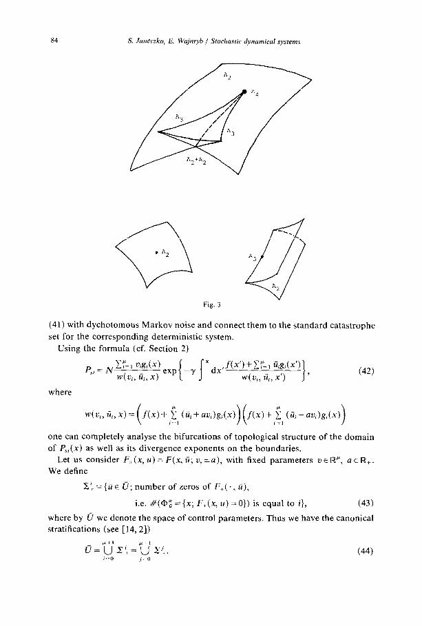
84 S. Janeczko, E. Wajnryb / Stochastic dynamical systems
Fig. 3
(41) with dychotomous Markov noise and connect them to the standard catastrophe
set for the corresponding deterministic system.
Using the formula (cf. Section 2)
p = N CY=‘=l uigi(x) exp 5,
w("i, iii, xl 1 5 -Y x dx,f(X’)+Ztl Uigi(X’)
w(u,-, iii, x’) I ’ (42)
where
one can completely analyse the bifurcations of topological structure of the domain
of PSI(x) as well as its divergence exponents on the boundaries.
Let us consider F&(x, u) = F(x, U; 21, *a), with fixed parameters ZJ E RP, a E R,.
We define
I;: = {ti E 0; number of zeros of F,( . , U),
i.e. #(@z = {x; F+(x, u) = 0)) is equal to i}, (43)
where by lI? we denote the space of control parameters. Thus we have the canonical
stratifications (see [ 14,2])
I/=lijl,;=*;l,<. (44)
i=O j=O

S. Janeczko, E. Wajnryb / Stochastic dynamical systems 85
To each xz E @i we can associate +l (-1) if it is a local minimum or inflection
point of the potential V, (if it is a local maximum of V,). We denote this function
by sgn xt. Now we can define the function
x: l?+ NW(O), (45)
x(ti)=min f,i, (l+sgnx:),f i i
(l+sgnx;) 1
(46) k=l
where ii~Z:n;l;‘.
By straightforward calculations for our Ak-singularities of (41) (cf. [ 141) we have
the following result.
Proposition 5.1. For a generic stochastic system (41) and sufhciently small a > 0, the
integer-valued function x defines the topological type of the support of P,,. The value
of x measures the number of connected components of the support. x is equal to zero
tf and only if PS, is not defined at all. Discontinuities of x define the points of the
bifurcation diagram for the corresponding stochastic dynamical system.
We now illustrate the bifurcation diagram for the concrete perturbations of the
fold catastrophe and cusp catastrophe (cf. [14,4]).
Let us consider the system (the fold catastrophe)
x=x’-(C+u(t))=-grad, VI (47)
The two equilibrium surfaces for V+ and V- are shown in Fig. 4. Geometrical
analysis of the pairs of potentials V+, V_ corresponding to the regions (Y, /3, y, 6,
p as illustrated in Fig. 5 (cf. Remark 2.1) immediately gives the supports for integrable
Fig. 4

86 S. Janeczko, E. Wajnryb / Stochastic dynamical systems
Fig. 5
and thus physically accepted stationary probabilities (the dotted region in Fig. 4).
We easiIy check the topological type function x for this system
x(u) = 0, U < a,
1, C3a. (48)
Thus, U = a is a bifurcation point; the shifted one corresponding to the deterministic
fold catastrophe.
Remark 5.2. In the case of unstable systems, which are always induced from stable
ones by appropriate morphisms, say F 0 @(x, u) (cf. [4]), the function x gives only
an upper bound for the topological type of the support. As an example of such a
system we can take the Verhulst chemical reaction equation (cf. [9])
a=F(x, 27, U(t))=-X*+X(U+U(t)), (49)

S. Janeczko, E. Wajnryb / Stochastic dynamical systems 87
where the deterministic F is induced from the stable fold singularity F(x, U) =
-x2+ U by the morphism Q(x, ti) = (x -$G, $Z4), i.e. F = F 0 @. We can easily check
that x(17) = 1 but the existence of an integrable P,, only occurs for U 3 0.
Let us consider the system (41) on the plane, p = 2, with direction of fluctuations
u = (0, l), i.e. f = -x3 - U,x - (I& + u(t)). The corresponding stratifications of C? are
2:: {A,>O}, (50)
2:: {A, = 01, (51)
2:: {A,<O}, (52)
I B
Fig. 6
x -l(2) -B
Fig. 7
88 S. Janeczko, E. Wojnryb / Stochastic dynamical systems
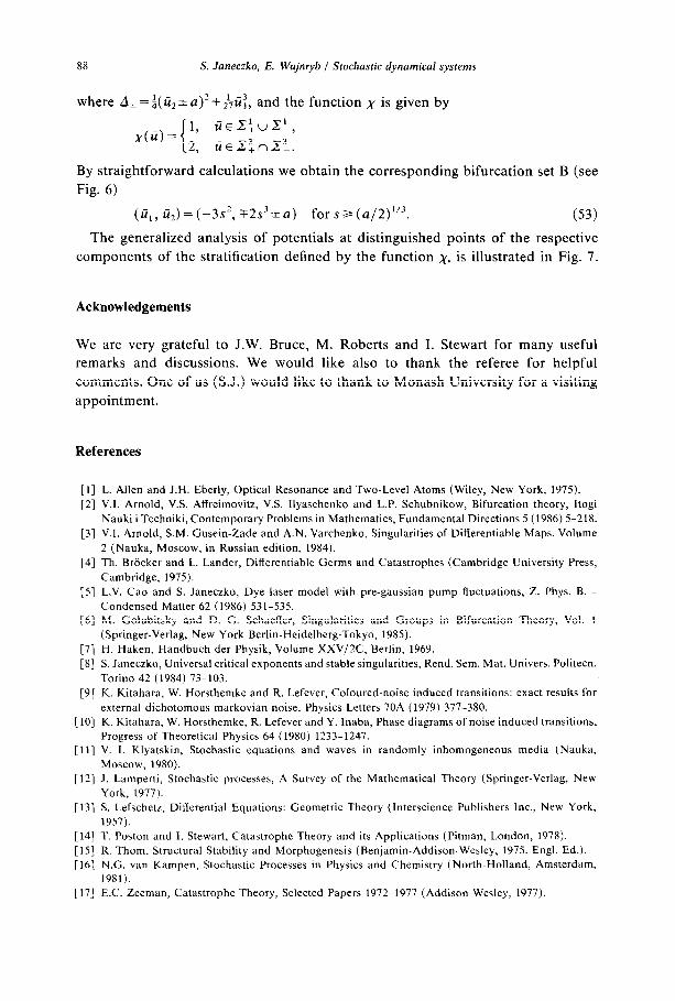
where A, = a( ii,* a)‘+$$, and the function x is given by
By straightforward calculations we obtain the corresponding bifurcation set B (see
Fig. 6)
(Ui, ii2) = (-3s2, r2s3 * a) for s 2 (a/2)“‘.
The generalized analysis of potentials at distinguished points of the respective
components of the stratification defined by the function x, is illustrated in Fig. 7.
Acknowledgements
We are very grateful to J.W. Bruce, M. Roberts and I. Stewart for many useful
remarks and discussions. We would like also to thank the referee for helpful
comments. One of us (S.J.) would like to thank to Monash University for a visiting
appointment.
References
[l] L. Allen and J.H. Eberly, Optical Resonance and Two-Level Atoms (Wiley, New York, 1975).
[2] V.I. Arnold, VS. Affreimovitz, VS. Ilyaschenko and L.P. Schubnikow, Bifurcation theory, Itogi
Nauki i Techniki, Contemporary Problems in Mathematics, Fundamental Directions 5 (1986) 5-218.
[3] V.I. Arnold, SM. Gusein-Zade and A.N. Varchenko, Singularities of Differentiable Maps. Volume
2 (Nauka, Moscow, in Russian edition, 1984).
[4] Th. Brocker and L. Lander, Differentiable Germs and Catastrophes (Cambridge University Press,
Cambridge, 1975).
[5] L.V. Cao and S. Janeczko, Dye laser model with pre-gaussian pump fluctuations, Z. Phys. B. -
Condensed Matter 62 (1986) 531-535. [6] M. Golubitsky and D. G. Schaeffer, Singularities and Groups in Bifurcation Theory, Vol. 1
(Springer-Verlag, New York-Berlin-Heidelberg-Tokyo, 1985).
[7] H. Haken, Handbuch der Physik, Volume XXV/2C, Berlin, 1969.
[8] S. Janeczko, Universal critical exponents and stable singularities, Rend. Sem. Mat. Univers. Politecn.
Torino 42 (1984) 73-103.
[9] K. Kitahara, W. Horsthemke and R. Lefever, Coloured-noise induced transitions: exact results for
external dichotomous markovian noise, Physics Letters 70A (1979) 377-380. [IO] K. Kitahara, W. Horsthemke, R. Lefever and Y. Inaba, Phase diagrams of noise induced transitions,
Progress of Theoretical Physics 64 (1980) 1233-1247. [ll] V. 1. Klyatskin, Stochastic equations and waves in randomly inhomogeneous media (Nauka,
Moscow, 1980).
[12] J. Lamperti, Stochastic processes, A Survey of the Mathematical Theory (Springer-Verlag, New
York, 1977). [ 131 S. Lefschetz, Differential Equations: Geometric Theory (Interscience Publishers Inc., New York,
1957). [14] T. Poston and I. Stewart, Catastrophe Theory and its Applications (Pitman, London, 1978).
[15] R. Thorn, Structural Stability and Morphogenesis (Benjamin-Addison-Wesley, 1975. Engl. Ed.).
[16] N.G. van Kampen, Stochastic Processes in Physics and Chemistry (North-Holland, Amsterdam, 1981).
[17] E.C. Zeeman, Catastrophe Theory, Selected Papers 1972-1977 (Addison-Wesley, 1977).