bifurcation phenomena and attractive periodic solutions in the
TRANSCRIPT

Bifurcation phenomena and attractive periodic
solutions in the saturating inductor circuit
Michele V. Bartuccelli∗, Jonathan H.B. Deane∗, Guido Gentile†
∗Department of Mathematics, University of Surrey, Guildford, GU2 7XH, UK.
E-mails: [email protected], [email protected]†Dipartimento di Matematica, Universita di Roma Tre, Roma, I-00146, Italy.
E-mail: [email protected]
Abstract
In this paper we investigate bifurcation phenomena, such as those of the periodicsolutions, for the “unperturbed” nonlinear system G(x)x + βx = 0, with G(x) =(α + x2)/(1 + x2) and α > 1, β > 0, when we add the two competing terms−f(t) + γx, with f(t) a time-periodic analytic “forcing” function and γ > 0 thedissipative parameter. The resulting differential equation G(x)x+βx+γx−f(t) = 0describes approximately an electronic system known as the saturating inductorcircuit. For any periodic orbit of the unperturbed system we provide conditionswhich give rise to the appearance of subharmonic solutions. Furthermore we showthat other bifurcation phenomena arise, as there is a periodic solution with thesame period as the forcing function f(t) which branches off the origin when theperturbation is switched on. We also show that such a solution, which encircles theorigin, attracts the entire phase space when the dissipative parameter becomes largeenough. We then compute numerically the basins of attraction of the attractiveperiodic solutions by choosing specific examples of the forcing function f(t), whichare dictated by experience. We provide evidence showing that all the dynamics ofthe saturating inductor circuit is organised by the persistent subharmonic solutionsand by the periodic solution around the origin.
1 Introduction
One of the most important second-order linear systems in practical applications is thenon-autonomous simple harmonic oscillator, which is described by
Lx + Rx + x/C = f(t), (1.1)
with L, R and C constants. This is the standard linear, second-order, constant coef-ficient ODE with nonzero right hand side. In an electronics context, the well-knowninductor-resistor-capacitor circuit is described by exactly this differential equation, pro-vided that the inductor (L), resistor (R) and capacitor (C) are all independent of x,which in this case would be the charge on the capacitor. In many cases, this is anexcellent approximation. However, a non-linear capacitor can easily be implemented
1
in practice, for instance, by using a semi-conductor diode, and the resulting nonlineardifferential equation has been studied in detail in the case where x does not change signin [5], [3]. Another practical but rather less studied nonlinear version of equation (1.1)is one in which R and C are constant but L is a function of x. Model L(x) functionsare of course based on practical experience. Practical inductors consist of a length ofwire wound around a core of magnetisable material, real materials being capable of sat-uration (so that L is a function of x, as will become clear) and possibly also displayinghysteresis (so that L is a function of x and x). Hence, the behaviour of real inductorscan depart from the ideal, constant L. A simple and not very realistic model of sat-uration was studied in [9], where an even, piecewise constant L(x) = L0 if |x| < X,L = L1 otherwise, with L0 > L1, was used. In a bid for a more faithful model of realinductors, a comparison between experiment and simulation was reported in [10], whereboth saturation and hysteresis effects were considered. The resulting system was de-scribed by a third order nonautonomous nonlinear ODE, which was solved numericallyand compared with experiment.
In this paper, we study a model which lies between the two extremes describedabove: an inductor whose core saturates, this time smoothly, but which does not displayhysteresis.
The rest of the paper is organised as follows. In Section 2, under appropriate as-sumptions and approximations, we derive and rescale the equation that we study. Suchan equation appears as a perturbation of an integrable equation, whose main propertieswill be reviewed in Section 3. We then study the periodic solutions of the full unper-turbed equation. First, in Section 4 we investigate the persistence of periodic solutionsof the unperturbed system which are “in resonance” with the forcing term (the so-calledsubharmonic solutions). Then in Section 5 we show that the system is characterised bythe presence of another periodic solution, which has the same period as the forcing andencircles the origin. More precisely it branches off the origin in the sense that it reducesto the origin when the forcing is removed. Therefore such a solution is different in aprofound way from the subharmonic solutions, because it arises by bifurcation from thestable equilibrium point and not from the unperturbed periodic solutions. The periodicsolution encircling the origin has a non-empty basin of attraction which becomes theentire phase space when the dissipative parameter is large enough; this will be provedin Section 6. In principle there could be other solutions relevant for the dynamics.However there is strong numerical evidence that the full dynamics is organised by theperiodic solutions that we have studied analytically. In fact, the numerical simulationsperformed in Section 7 suggest that the union of the basins of attraction of those pe-riodic solutions fills the entire phase space; cf. [6, 1] for similar situations. Finally, inSection 8 we draw some conclusions, and discuss some open problems and possible linesof future research.
2 The saturating inductor circuit ODE
The circuit under consideration is shown in figure 1 and we now derive the ODE thatdescribes it, briefly explaining the assumptions that we make. Details of the electro-
2

g(ωt)
q(t)
i = q
L(i)
D/2
(a)
(b)
vR
vL
vCC
RA
Figure 1: (a) The saturating inductor circuit driven by a voltage source g(ωt) is describedby the ODE discussed in this paper. In this diagram, the dependent variable, the capacitorcharge, is q(t); the current, i(t) = q(t); C (capacitance) and R (resistance) are constants andL = L(q) = L(i) is the nonlinear inductance. The voltages across the inductor, resistor andcapacitor are vL, vR and vC respectively. (b) The core of the saturating inductor, with cross-sectional area A and mean diameter D.
magnetism and circuit theory required can be found in [18]. Kirchhoff’s voltage lawstates that the sum of the voltages across the components must equal the applied volt-age at all times, and so g(ωt) = vL + vR + vC . The definition of capacitance statesthat vC = q(t)/C, where q(t) is the capacitor charge; also by definition, the currenti(t) = q(t); and Ohm’s law allows us to write vR = i(t)R. Faraday’s law of inductionstates that vL = dφ/dt where φ is the magnetic flux, to be defined. To proceed further,we need to make assumptions about the geometry of the inductor core. In order thatit will display saturation at relatively low currents, we assume that it is toroidal inshape, with cross sectional area A and mean diameter D, and that the inductor itselfconsists of n turns of wire around this core. The magnetic flux density is defined byB = µ0(H + M), where µ0 = 4π × 10−7 is the permeability of free space, H is theapplied magnetic field and M is the magnetisation. In fact, the quantities B, H and Mare all vectors, but under the assumption that they are all parallel to each other andnormal to the cross-section of the core, we shall see that we need only consider theirmagnitudes. The magnetic flux is then defined by
φ = n
∫∫
BdA = nµ0
∫∫
(H + M)dA = nµ0A(H + M).
3

Now, Ampere’s circuital law relates H to i by H = ni/πD, and so
dφ
dt=
di
dt
dφ
di= q
dφ
di=
µ0n2A
πDq
(
1 +dM
dH
)
. (2.1)
We now need a model for M(H). In the absence of hysteresis, and with weak couplingbetween the magnetic domains, M(H) is usually described by the Langevin function
M(H) = Ms [coth(H/a) − a/H] , where limH→0
M(H) = 0,
and where Ms > 0 and a > 0 are constants which depend on the core material. Now,
dM
dH=
Ms
a
[
1 − coth2
(
H
a
)
+a2
H2
]
≡ U
(
H
a
)
,
where
limH→0
dM
dH=
Ms
3a, lim
H→±∞
dM
dH= 0.
Using this in equation (2.1), and Kirchhoff’s voltage law, allows us to write the differ-ential equation that describes the circuit as
µ0n2A
πD
[
1 + U
(
nq
πDa
)]
d2q
dt2+ R
dq
dt+
q
C= g(ωt) (2.2)
and all the coefficients are well-defined even when q = 0. We now rescale time byreplacing ωt with t, and q by defining ωnq(t) = πDaλx(t), with λ a constant to bedefined, giving
x [1 + U(λx)] + γx + βx = f(t), (2.3)
where
γ =πDR
µ0n2ωA, β =
πD
µ0n2ω2AC, f(t) =
g(t)
µ0nωλaA. (2.4)
Finally, we can usefully approximate the function U with an expression that isqualitatively similar but easier to handle analytically. From the foregoing, we have, forall λ, that limy→±∞ 1 + U(λy) = 1 and limy→0 1 + U(λy) = 1 + Ms/(3a) ≡ α > 1. Thesimplest rational approximation to 1 + U(λy) which has the same limits (independentof λ) is L(y) = (α+y2)/(1+y2). Since we are free to choose λ, we find the value λ = λ0
that minimises
I(α, λ) =
∫ ∞
0
[
1 + 3(α − 1)(
1 − coth2(λy) + 1/(λy)2)
− α + y2
1 + y2
]2
dy
= (α − 1)2∫ ∞
0
[
3(
1 − coth2(λy) + 1/(λy)2)
− 1
1 + y2
]2
dy.
Numerical computation gives the value λ0 ≈ 1.99932.
Hence we set λ = λ0 and using the resulting approximation for the function U , thedifferential equation in its final form is
x = y,α + y2
1 + y2y = f(t) − γy − βx. (2.5)
4
In the rest of the paper we shall be interested in investigating how the dynamicsof the “unperturbed” system x = y, (α + y2)/(1 + y2)y = −βx will be influenced bythe addition of the two competing terms f(t) − γy under the assumption that theyrepresent a “small” perturbation. We shall be able also to investigate cases far fromthe perturbation regime, at least when the dissipative parameter is large enough withrespect to the forcing term.
3 The unperturbed system
Consider the ordinary differential equation (we set γ = εC for notational convenience)
x = y, y = −g(y)x +ε
β
(
g(y)(f(t) − Cy))
, (3.1)
where g(y) = β(1 + y2)/(α + y2), with α > 1, f(t) = f(t + 2π) is a analytic periodicfunction of time, and ε (small), C ≥ 0 are two real parameters. Without loss we canredefine our ε so as to absorb the positive constant β. For ε = 0 our system is integrableby quadratures; in fact it has an integral of motion, which we identify with its energy,given by
E(x, y) =1
β
(
y2
2+
α − 1
2log(1 + y2)
)
+x2
2. (3.2)
Note that the above system is a particular case of the following class of systemspossessing an integral of motion: x = y, y = −g(y)F (x), the associated integral beinggiven by
∫
y
g(y)dy +
∫
F (x) dx.
The following result is proved in Appendix A.
Lemma 1 Consider the system (3.1) with ε = 0. Its phase space is filled with periodicorbits around the origin; the period T0 of these orbits is strictly decreasing as a functionof the energy (3.2), and satisfies the inequalities 2π/
√β < T0 < 2π
√
α/β.
For ε = 0 the system (3.1), in the limits of small and large energy, becomes “es-sentially” the harmonic oscillator with frequencies ω = 1/
√α and ω = 1 respectively.
We observe that for any fixed value of the energy we have formally an infinite numberof unperturbed periodic solutions parametrized by a phase shift t0. This phase shift isirrelevant in the autonomous case (ε = 0), but becomes very important when we addthe time dependent perturbation (ε 6= 0), because in the extended phase space (x, y, t)each “initial” phase will give rise to a different orbit. Therefore the unperturbed so-lution to be continued for ε 6= 0 can be written in terms of the initial phase, in theform x0(t) = X0(t − t0), where X0(t) is an unperturbed solution with the phase ap-propriately fixed (for instance with X0(0) = 0) in order to impose some constraints onthe perturbed system (see below). For practical purposes it will be more convenient tochange the origin of time, by writing the unperturbed solution as x0(t) = X0(t) and theperiodic forcing function in the form f(t + t0).
5

Lemma 2 Consider the system (3.1) with ε = 0. The energy function (3.2) satisfiesthe identities E(±x,±y) = E(x, y). The solutions x0(t) can be chosen to be even in t,and satisfy x0(t) = −x0(t − T0/2), if T0 is the corresponding period. Furthermore theypossess only odd components in their Fourier series expansion.
Proof. The equation (3.2) shows that the energy function is even in both variables (x, y),namely E(±x,±y) = E(x, y). Therefore the solutions (x0(t), y0(t)) have reflectionalsymmetry with respect to both axes (x, y). Hence giving initial conditions on the x-axis one obtains solutions x0(t) which are even in time (similarly if one chooses initialconditions on the y-axis then the solutions are odd in time). Using this property itfollows that any solution of period T0 can be chosen to be even in time, and moreoverit must have the property x0(t) = −x0(t − T0/2).
To show the validity of the part concerning the Fourier spectrum, consider theFourier series of x0(t), namely
x0(t) =∑
ν∈Z
x0νeiνωt, (3.3)
where ω = 2π/T0. The Fourier coefficients can be written as
T0 x0ν =
∫ T0
0dt e−iνωtx0(t) =
∫ T0/2
0dt e−iνωtx0(t) −
∫ T0
T0/2dt e−iνωtx0
(
t − T0
2
)
=
∫ T0/2
0dt e−iνωtx0(t) − e−iνωT0/2
∫ T0/2
0dt′ e−iνωt′x0(t
′)
= (1 − e−iνπ)
∫ T0/2
0dt e−iνωtx0(t).
Therefore if ν is an even number (including zero) x0,ν = 0, while if ν is an odd numberx0,ν 6= 0.
We now investigate the dynamics of the system when ε 6= 0 (and small). In particularwe are interested in studying which periodic orbits of the unperturbed system persistunder the combined effect of the periodic perturbation f(t+ t0) = f(t+ t0 +2π) and thedissipative term Cx; cf. [1, 8, 15, 16, 19, 14] for related results. Notice that in order tohave a periodic solution with period commensurate with 2π we must impose a so-calledresonance condition given by ω = 2π/T0 = p/q. If ω satisfies the above condition thenthe perturbed periodic solution will have the period T = pT0, during which the periodicforcing function f(t + t0) has “rotated” q times. Notice that the phase t0 ∈ [0, 2πq/p).It is more convenient to consider the system
x = y, y = −g(y)x +ε
β
(
g(y)(f(t) − Cx))
, t = 1, (3.4)
defined in the extended phase space (x, y, t). Then for ε = 0 the motion of the variables(x, y, t) is in general quasi-periodic, and reduces to a periodic motion whenever T0
becomes commensurate with 2π. Thus in the extended phase space (x, y, t) the solution
6

runs on an invariant torus which is uniquely determined by the energy E; if ω = p/qwe say that the torus is resonant. In general the non-resonant tori disappear under theeffect of the perturbation, unless the system belongs to the class which can be analyzedby using the KAM theory. Also the resonant tori disappear, but some remnants are left:indeed usually a finite number of periodic orbits, called subharmonic solutions, lying onthe unperturbed torus, can survive under the effect of the perturbation. If ω = p/q weshall call q/p the order of the corresponding subharmonic solutions. The subharmonicsolutions will be studied in Section 4.
Besides the subharmonic solutions, there are other periodic solutions which arerelevant for the dynamics: indeed there is a periodic solution branching off the origin.This is a feature characteristic of forced systems in the presence of damping [2, 3, 12].Existence and properties of such a solution will be studied in Sections 5 and 6. Inparticular we shall show that this periodic solution becomes a global attractor if thedissipative parameter is large enough.
4 Subharmonic solutions
We consider the system (3.1) with ε 6= 0 and small, and we look for subharmonicsolutions which are analytic in ε. First, we formally define power series in ε of the form
x(t) =
∞∑
k=0
εkx(k)(t), y(t) =
∞∑
k=0
εky(k)(t), C =
∞∑
k=0
εkCk, (4.1)
where the functions x(k)(t) and y(k)(t) are periodic with period T = pT0 = 2πq for allk ∈ N. We shall see that the functions x(k)(t) and y(k)(t) can be determined providedthe parameters Ck are chosen to be appropriate functions of the initial phase t0.
If we introduce the decompositions (4.1) into (3.1) and we denote with W (t) theWronskian matrix for the unperturbed linearised system, we obtain
(
x(k)(t)
y(k)(t)
)
= W (t)
(
x(k)
y(k)
)
+ W (t)
∫ t
0dτ W−1(τ)
(
0
F (k−1)(τ)
)
, (4.2)
where (x(k), y(k)) are corrections to the initial conditions, and
F (k)(t) =
∞∑
m=0
∑
r1,r2∈Z+
r1+r2=m
1
r1!r2!
∂r1
∂yr1
∂r2
∂Cr1F (y0, C0, t + t0) ×
×∑
k1+...+km=k
y(k1)(t) . . . y(kr1)(t)Ckr1+1
. . . Ckm. (4.3)
where F (y, C, t+t0) = g(y) (f(t + t0) − Cy). Note that by construction F (k)(t) dependsonly on the coefficients y(k′)(t) and C(k′) with k′ ≤ k.
We shall denote by (x0, y0) the solution of the unperturbed system x0 = y0, y0 =−g(y0)x0, with x0 even (hence y0 odd): this is possible by Lemma 1. The Wronskian
7
matrix appearing in (4.2) is a solution of the unperturbed linear system
W (t) = M(t)W, M(t) =
(
0 1−g(y0) −(∂g(y0)/∂y)x0
)
(4.4)
so that the matrix W (t) can be written as
W (t) =
(
c1∂x0/∂E c2x0
c1∂y0/∂E c2y0
)
, (4.5)
where c1 and c2 are suitable constant such that W (0) = 1 (one easily check thatc1c2 = −α).
By making explicit the dependence on E of the unperturbed periodic solutions, wecan write
x0(t) = x0(ω(E)t, E) =∑
ν
xν(E) eiνω(E)t, (4.6)
so that we can write
∂x0
∂E=
∂ω(E)
∂Et h(t) + b(t), x0(t) = ω(E)h(t),
where
h(t) =∑
ν
iν xν(E) eiνω(E)t, b(t) =∑
ν
∂xν(E)
∂Eeiνω(E)t.
Note in particular that h(t) and b(t) are, respectively, odd and even in t, so that ∂x0/∂Eis even in time.
Hence we have
∂x0
∂E= µtx0 + b(t), µ =
1
ω(E)
∂ω(E)
∂E,
where µ 6= 0 because the system is anysochronous and the derivative of the perioddT0(E)/dE < 0 as shown in Lemma 1; also the functions h(t), b(t), x0(t) are periodicwith period T0. Notice that the lower two components of the Wronskian are the timederivatives of the upper two. Hence we can express the Wronskian as follows:
W (t) =
(
c1 (µtx0(t) + b(t)) c2x0(t)
c1
(
µx0(t) + µtx0(t) + b(t))
c2x0(t)
)
. (4.7)
By introducing (4.7) in (4.2) and using that
det W (t) = c1c2
(
y0∂x0
∂E− x0
∂y0
∂E
)
= − c1c2
G(y0)
(
x0∂x0
∂E+ y0G(y0)
∂y0
∂E
)
= − c1c2
G(y0),
we obtain for all k ≥ 1
x(k)(t) = c1(µx0(t)t + b(t))x(k) + c2x0(t)y(k) + (µx0(t)t + b(t)) ×
×∫ t
0dτ G(y0(τ))x0(τ)F (k−1)(τ) − x0(t)
∫ t
0dτ G(y0(τ))(µx0(τ)τ + b(τ))F (k−1)(τ),
8

where G(y) = (α+y2)/(β(1+y2)); a similar expression can be written for the componenty(k)(t) = x(k)(t). After some manipulation we obtain
x(k)(t) = c1
(
µtx0(t)x(k) + b(t)x(k)
)
+ c2x0(t)y(k) + b(t)
∫ t
0dτ G(y0(τ))x0(τ)F (k−1)(τ)
−x0(t)
∫ t
0dτ G(y0(τ))b(τ)F (k−1)(τ) + µx0(t)
∫ t
0dτ
∫ τ
0dτ ′G(y0(τ
′))x0(τ′)F (k−1)(τ ′).
For notational convenience let us put Φ(k−1)(t) = G(y0(t))x0(t)F(k−1)(t), F (k−1)(t) =
∫ t0 dτ Φ(k−1)(τ) and Ψ(k−1)(t) = G(y0(t))b(t)F
(k−1)(t). Then we obtain a periodic solu-tion of period T = pT0 = 2πq if, to any order k ∈ N, one has
〈Φ(k−1)〉 :=1
T
∫ T
0dτ Φ(k−1)(τ) = 0, c1x
(k) =〈Ψ(k−1)〉
µ− 〈F (k−1)〉, (4.8)
where, given any T -periodic function H we denote its mean by 〈H〉. Also recall thatµ 6= 0 and c1 6= 0.
The parameters y(k) are left undetermined, and we can fix them arbitrarily, as theinitial phase t0 is still a free parameter. For instance we can set y(k) = 0 for all k ∈ N
or else we can define y(k) = y(k)(t0) for k ∈ N, with the values y(k)(t0) to be fixed inthe way which turns out to be most convenient [14].
Thus, under the restrictions (4.8) we have that for all k ≥ 1
x(k)(t) = c1b(t)x(k) + c2x0(t)y
(k) + b(t)
∫ t
0dτ Φ(k−1)(τ) (4.9)
+
∫ t
0dτ(
Ψ(k−1)(τ) − 〈Ψ(k−1)〉)
+ µx0(t)
∫ t
0dτ(
F (k−1)(τ) − 〈F (k−1)〉)
is a periodic function of time. Hence we must prove that the first condition in (4.8) canbe fulfilled at all orders k ≥ 1; the second condition just gives a prescription how to fixthe parameters x(k).
For k = 1 the condition on the zero average, in terms of the Melnikov integral (noticethat G(y0(τ))g(y0(τ)) = 1)
M(t0, C0) :=
∫ T
0dτ G(y0(τ))x0(τ)F (0)(τ)=
∫ T
0dτ x0(τ)
[
− C0x0(τ) + f(τ + t0)]
gives M(t0, C0) = 0, and we can choose C0 = C0(t0) so that this holds because
∂M(t0, C0(t0))
∂C0= −
∫ T
0dτ [x0(τ)]2 := −D 6= 0
for all t0 ∈ [0, 2πq/p).
For k = 2 the condition reads (recall that x0 = y0)
C1 =1
DΓ(1)(C0, x0, x
(1), y0, y(1), t0) =
1
D
∫ T
0dτ G(y0(τ))x0(τ) ×
×[
− C0y(1)(τ)x0(τ)g′(y0(τ))x(1)(τ)x0(τ)y(1)(τ)
−g′′(y0(τ))
2x0(τ)x0(τ)(y(1))2(τ) + g′(y0(τ))x0(τ)y(1)(τ)f(τ + t0)
]
,
9

where the primes denote differentiation with respect to y. For higher values of k, inorder to satisfy the first condition in (4.8) we must choose
Ck =1
DΓ(k)(C0, . . . , Ck−1, x0, . . . , x
(k), y0, . . . , y(k), t0), (4.10)
where Γ(k) can be proved, by induction, to be a well-defined periodic function dependingon the coefficients C0, . . . , Ck−1, x0, . . . , x
(k), y0, . . . , y(k). Therefore we conclude that if
we set C0 = C0(t0) and, for all k ≥ 1, we choose y(k) = y(k)(t0), x(k) according tothe second condition in (4.8) and Ck = Ck(t0) according to (4.10), we obtain that inthe series expansions (4.1) the coefficients x(k)(t) and y(k)(t) are well-defined periodicfunctions of period T . All of this of course makes sense if the series expansions (4.1)converge; this can be seen by showing that the coefficients admit bounds of the form|x(k)(t)| < δk for some positive constant δ; hence by taking ε small enough and C =C(ε, t0) as a function of t0 according to (4.10) it follows that the series converges to aperiodic function with period T = T0p, analytic in t and ε. The strategy for showingthe convergence of the series is essentially the same as that explained in [11, 14], andall the details can be found in these references. So the formal power series convergesfor |ε| < ε0 = δ−1. For fixed ε ∈ (−ε0, ε0) we shall find the range allowed for C bycomputing the supremum and the infimum, for t0 ∈ [0, 2π), of the function t0 → C(ε, t0).The bifurcation curves will be defined in terms of the function C(ε, t0) as
γ1(ε) = ε supt0∈[0,2π)
C(ε, t0), γ2(ε) = ε inft0∈[0,2π)
C(ε, t0). (4.11)
These bifurcation curves divide the parameter plane (ε, γ) into two disjoint sets suchthat only inside the region delimited by the bifurcation curves are there subharmonicsolutions; the region of existence contain the real ε−axis. For more details on this pointsee [14].
We are now in a position to summarise the above discussion by stating the followingtheorem which is an adaptation of Theorem 5 of [14].
Theorem 1 Consider the system (3.1). There exist ε0 > 0 and two continuous func-tions γ1(ε) and γ2(ε), with γ1(0) = γ2(0), γ1(ε) ≥ γ2(ε) for ε ≥ 0 and γ1(ε) ≤ γ2(ε)for ε ≤ 0, such that (3.1) has at least one subharmonic solution of period 2πq forγ2(ε) ≤ εC ≤ γ1(ε) when ε ∈ (0, ε0) and for γ1(ε) ≤ εC ≤ γ2(ε) when ε ∈ (−ε0, 0).
The above theorem applies for any analytic 2π-periodic forcing function of time;so, provided that the integers p, q are relatively prime, it follows that generically anyresonant torus of the system (3.1) possesses subharmonic solutions of order q/p. Nat-urally if we choose a particular forcing function with special properties, then in turnthis will influence the set of possible subharmonic solutions. For example if we takethe function f(t) = sin t then for dissipation large enough — that is for γ = O(ε) —the only existing subharmonic solutions are those with frequency ω = 1/(2k + 1) withk any positive integer. This can be seen as follows. The solutions of the unperturbedsystem have odd components only in their Fourier representation; moreover we know
10
that to first order the Melnikov condition M(t0, C0) = 0 must be satisfied. Hence wecan choose
C0(t0) =
∫ T0 dτ x0(τ)f(τ + t0)∫ T0 dτ [x0(τ)]2
, (4.12)
which is well defined because the denominator is non zero; hence by computing theintegral in the numerator of (4.12) by using the Fourier representations of x0 and f(t) =sin t and by taking the zero Fourier component of their product one can see that theonly possible frequencies are of the type ω = 1/(2k + 1); see [1] for details. We are
implicitly assuming that the integral∫ T0 dτ x0(τ)f(τ + t0) is non-zero; this must be
checked (either analytically or numerically), because if it happens to be zero then wehave to go to higher orders until we find a k > 1 such that
Ck =1
∫ T0 dτ [x0(τ)]2
Γ(k)(C0, . . . , Ck−1, x0, . . . , x(k), y0, . . . , y
(k), t0) 6= 0. (4.13)
Other subharmonic solutions appear only for much smaller values of the dissipativeparameter, that is for γ = O(εp), with p > 1. Again we refer to [1, 14] for furtherdetails.
The subharmonic solutions turn out to be attractive. The numerical analysis per-formed in Section 7 gives evidence that, at least for small values of the perturbationparameter ε, all trajectories in phase space are eventually attracted either to some sub-harmonic solution or to the periodic solution which will be investigated in Section 5.Notice that this situation is different from the kind of problem studied in [20]: first ofall our unperturbed system is strongly nonlinear; moreover, the limit cycles describedby the attractive periodic solutions are generated by the perturbation itself, so that theproblem does not consist in studying the persistence of the self-sustained limit cycle.
5 Periodic solution branching off the origin
In this section we wish to investigate the periodic solution which originates from thezero solution in the presence of the periodic forcing function f(t) = f(t + 2π). For thisit is more convenient to write our system as follows:
x = y, y = −g(y)x − γg(y)x + εg(y)f(t), (5.1)
where g(y) = β(1 + y2)/(α + y2), and again the constant β has been absorbed into theconstants ε and γ.
The following result will be proved.
Theorem 2 Consider the system (5.1), and assume that Q0 = minn∈N |n2 −α/β| 6= 0.There exists ε0 ∝ max{γ,Q0} such that for |ε| < ε0 the system (5.1) admits a periodicsolution x0(t) with the same period as the forcing, which describes a closed curve C ofdiameter O(ε/ε0) around the origin. Moreover for any value of ε there exists γ0 > 0such that for γ > γ0 the periodic solution x0(t) describes a global attractor.
11

The idea is to expand the periodic solution around the origin and then to use asimilar strategy to the one of the previous section. Thus we have
x(t) =∞∑
k=1
εkx(k)(t), y(t) =∞∑
k=1
εky(k)(t), g(y) =∞∑
k=0
1
k!
dkg
dyk(0) yk; (5.2)
notice that the dissipative parameter γ is now included in the “unperturbed” system andtherefore it is (in general) not necessarily small. We now introduce the decompositions(5.2) into (5.1) and we perform a similar analysis to that of Section 5. To first order inε we obtain (remember that the zero order solution is the origin)
x(1) + g(0)(
x(1) + γx(1))
− g(0)f(t) = 0, (5.3)
where g(0) = β/α. This equation is linear non-homogeneous and its time-asymptoticsolution (obtained by setting to zero the transient non-periodic part which decays ex-ponentially in time) has Fourier coefficients
x(1)ν =
g(0)fν
g(0)(1 + iγν) − ν2. (5.4)
In particular it has the same period as f . Notice that the first order solution x(1)(t)has the same average as the forcing function f(t) (as it should). It is now instructiveto compute the second order in ε and then the k-th order, because at second order onecan already see the general properties of the structure of the solution at any order. Byequating powers of ε2 we obtain
x(2) + g(0)(
x(2) + γx(2))
− g′(0)(
x(1)f(t) − x(1)x(1) − γ(x(1))2)
= 0, (5.5)
which can be easily solved in Fourier space.
By inspecting the structure of equation (5.1) one can see that at any order k thelinearised part is the same – compare for instance (5.3) with (5.5), – and the perturbationis formed of terms which are periodic functions having the same period as the forcingterm f(t); hence the structure of the equation at order k has the form
x(k) + g(0)(
x(k) + γx(k))
= P (k)(x(1), . . . , x(k−1), y(1), . . . , y(k−1), γ), (5.6)
where the function P (k) is a periodic function having the same period as the forcingterm f(t); hence, by writing
x(k)(t) =∑
ν∈Z
x(k)ν eiνt,
P (k)(x(1)(t), . . . , x(k−1)(t), y(1)(t), . . . , y(k−1)(t), γ),=∑
ν∈Z
P (k)ν eiνt, (5.7)
we find that the Fourier coefficients x(k)ν are given by
x(k)ν =
g(0)P(k)ν
g(0)(1 + iγν) − ν2, (5.8)
12

according to (5.6). Notice that P(k)ν depends on the coefficients x
(k′)ν′ , with k′ < k and
ν ′ ∈ Z, so that it is a well-defined periodic function (as can be checked by induction).
The explicit expression for P(k)ν can be found in Appendix B.
The convergence of the perturbation series (5.2) can be discussed as in the refer-ences [11, 14] quoted in the previous sections. The presence of the factor γ appearingin the denominator of (5.8) implies that the corresponding radius of convergence in εgrows linearly in γ. More precisely, by iterating (5.8) for every k down to k = 1, onefinds that, uniformly in t, |x(k)(t)| ≤ A(B/Q(γ))k−1, where A and B are constant whichdepends upon the functions g(y) and f(t), but not on γ, and Q(γ) = max{g(0)γ,Q0},with Q0 = minn∈N |g(0)−n2|; cf. Appendix B. Therefore by looking at the power seriesexpansion (5.2) one sees that by choosing ε judiciously the series converges. The radiusof convergence becomes smaller with decreasing γ up to a threshold value proportionalto 1/Q0 = 1/minn∈N |n2 − β/α|, below which it remains constant. For γ = 0 we canchoose Q0/B as the radius of convergence of the power series, provided n2 − β/α 6= 0(absence of resonances). Moreover, under this hypothesis, for any fixed ε — not nec-essarily small — we have that for γ large enough, say for γ > γ0, there is a periodicsolution x0(t) encircling the origin with the same period as the forcing. We shall seein the next section that there exists γ1 ≥ γ0 such that for γ > γ1 the solution x0(t)describes a global attractor.
6 Global attraction to the periodic solution encircling the
origin
In this section we wish to prove that if the dissipative parameter γ > 0 is large enoughthen every initial condition will evolve so as to tend asymptotically to the periodicsolution encircling the origin, whose existence was proved in the previous section. Westart with the perturbed equation in the form
G(x) x + x + γx − f(t) = 0, (6.1)
where G(y) = (α+y2)/(β(1+y2)), and the parameter ε (arbitrary: cf. the comments atthe end of the previous section) has been absorbed into the forcing function f(t). Thestrategy we follow is to split the solution x(t) = x0(t) + ξ(t), where x0(t) satisfies (6.1).Thus we must prove that ξ(t) → 0 as time goes to infinity. By introducing x(t) =x0(t) + ξ(t) into (6.1) and simplifying the terms satisfied by the periodic solution, weobtain the equation
G(x0 + ξ)(x0 + ξ) − G(x0)x0 + γξ + ξ = 0. (6.2)
We write it as
ξ = y, y = −g(x0 + ξ)[
−ξ − γξ −(
G(x0 + ξ) − G(x0))
x0
]
, (6.3)
where as usual g(x0 + ξ) = 1/G(x0 + ξ)). So we have to prove the following result.
13

Lemma 3 Consider the equation (6.3) with x0(t) the periodic solution encircling theorigin. Then if the dissipative parameter γ > 0 is large enough all trajectories in phasespace converge toward the origin asymptotically in time.
Proof. By using the Liouville-like transformation [4]
τ =
∫ t
0dt
√
g(x0 + ξ)
we first remove the time-dependence from the coefficient of ξ. We obtain: ξ =√
gξ′ and
ξ = gξ′′ + ξ′g′/2, where the prime denotes the derivative with respect to the variable τ .Substituting and simplifying we get
ξ′ = y, y′ = −ξ −(
γ√
g +g′
2g
)
ξ′ −(
G(x0 + ξ) − G(x0))
x0. (6.4)
By defining the Hamiltonian for the harmonic oscillator by H = (ξ2 +y2)/2 one can seethat H ′ = −Γy2 − Fy, where Γ = γ
√g + g′/(2g) and F = (G(x0 + ξ)− G(x0))x0. Now
one can see that we can estimate |G(x0 + ξ)−G(x0)| ≤ L|y| with L a positive constantof order 1/γ. The last property follows, when explicitly estimating L, from the factthat x0, x0, x0 are of order 1/γ (see (5.4)). Then one finds H ′ ≤ −y2(Γ − L/Γ) ≤ 0 forevery (ξ, y). Moreover H ′ = 0 only on the y-axis provided that γ is large enough. Sowe are in the hypotheses of the theorem of Barbashin-Krasovsky [17] and therefore wecan conclude that if γ is large enough so as to have γ
√g + g′/2g > 0 and Γ−L/Γ > 0 it
follows that the origin is asymptotically stable and it attracts all the solutions for everyinitial condition in phase space. This completes the proof of the lemma.
7 Numerical simulations
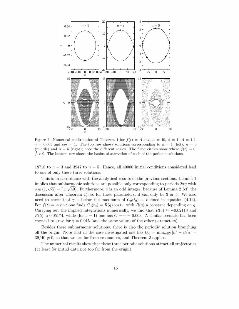
We now report on some numerical computations which illustrate Theorems 1 and 2 byconsidering a special case of equation (2.5) with f(t) = A sin t, and choosing A = 1.2,α = 40, β = 1 and γ = 0.003. Note that (2.5) corresponds to (3.1) with ε = 1.Technically Theorems 1 and 2, for fixed γ, have been proved for values of ε relativelysmall so as to be sure of the convergence of the power series that arise. However it is verytime consuming to obtain basin of attraction pictures for small values of the dissipativeparameter γ = εC. Hence, we have compromised by verifying, within the limitations offinite precision and time numerical computations, that only attracting periodic solutionshaving periods 2πn for n = 1, 3 and 5 exist, for (3.1) with ε = 1, ε = 0.1 and ε = 0.01.Only in the case ε = 1 have we computed the actual basins of attraction of each ofthese solutions — see figure 2. The figure shows solutions with periods 2πn for n = 1(left), n = 3 (middle) and n = 5 (right). Below these are the corresponding basins ofattraction. These were computed in the obvious way — by numerically integrating thedifferential equation starting from a set of initial conditions on a 200× 200 grid, and ineach case, after allowing the transient to decay sufficiently, deciding which solution hasbeen reached. Of the 40000 pixels in the figure, 17335 correspond to the n = 1 solution,
14
-0.04 -0.02 0 0.02 0.04x
-0.04
-0.02
0
0.02
0.04
y
-0.04 -0.02 0 0.02 0.04
-0.04
-0.02
0
0.02
0.04
-20 -10 0 10 20-20
-10
0
10
20
-20 -10 0 10 20-20
-10
0
10
20
-5 0 5-3
-2
-1
0
1
2
3
-30 0 30x
-15
0
15
y
n = 1 n = 3 n = 5
-30 0 30-15
0
15
-30 0 30-15
0
15
Figure 2: Numerical confirmation of Theorem 1 for f(t) = A sin t, α = 40, β = 1, A = 1.2,γ = 0.003 and eps = 1. The top row shows solutions corresponding to n = 1 (left), n = 3(middle) and n = 5 (right); note the different scales. The filled circles show where f(t) = 0,f > 0. The bottom row shows the basins of attraction of each of the periodic solutions.
18718 to n = 3 and 3947 to n = 5. Hence, all 40000 initial conditions considered leadto one of only these three solutions.
This is in accordance with the analytical results of the previous sections. Lemma 1implies that subharmonic solutions are possible only corresponding to periods 2πq withq ∈ (1,
√α) = (1,
√40). Furthermore, q is an odd integer, because of Lemma 2 (cf. the
discussion after Theorem 1), so for these parameters, it can only be 3 or 5. We alsoneed to check that γ is below the maximum of C0(t0) as defined in equation (4.12).For f(t) = A sin t one finds C0(t0) = R(q) cos t0, with R(q) a constant depending on q.Carrying out the implied integrations numerically, we find that R(3) ≈ −0.02113 andR(5) ≈ 0.05174, while (for ε = 1) one has C = γ = 0.003. A similar scenario has beenchecked to arise for γ = 0.015 (and the same values of the other parameters).
Besides these subharmonic solutions, there is also the periodic solution branchingoff the origin. Note that in the case investigated one has Q0 = minn∈N |n2 − β/α| =39/40 6= 0, so that we are far from resonances, and Theorem 2 applies.
The numerical results show that these three periodic solutions attract all trajectories(at least for initial data not too far from the origin).
15
8 Discussion and Conclusion
In this paper we have discussed various properties of the solutions of a nonlinear ODEwith periodic forcing, in which the nonlinearity consists, in a mechanical analogy, ofa velocity-dependent mass, the restoring force and dissipation being linear. The ODEarises as a model of an electronic circuit containing an inductor whose core saturates.The importance of this circuit is that it is very simple, consisting of only three electroniccomponents, and yet for certain values of the parameters can display chaotic behaviour.Previous studies made use of various simplified models of the saturating inductor: forinstance, by using a piecewise constant approximation to the function g(y) and neglect-ing hysteresis effects [9]; or by using a more realistic model including hysteresis effects(so that g depends on y and y) [10]. The latter results in a third-order nonautonomousODE [10]. The ODE studied in this paper is in between these two models, as it stillneglects hysteresis but uses a smooth — more realistic – function for the magnetisation.
In our analysis, we considered first the unperturbed version of the system in whichdissipation and forcing were absent, and showed that here, only periodic solutions aredisplayed and their period is a monotonically decreasing function of the energy. Whenthe perturbation is present, we have proved the existence of subharmonic solutions— that is solutions whose periods are rational multiples of the period of the forcing— and additionally, of a periodic solution with the same period as the forcing, thelatter becoming a global attractor in the presence of sufficient dissipation. Numericalcomputations have been carried out to illustrate this behaviour and show the relevanceof these solutions for the dynamics.
The main limitation in our model is the fact that we neglect hysteresis. On theother hand, as mentioned above, taking it into account leads to a much more com-plicated system, and application of the analysis techniques used here, at best, wouldrequire nontrivial generalisation. It would be interesting to investigate in a real circuitwhether hysteresis can be really neglected for certain inductor core materials. In generalthe results presented in [10] show that hysteresis produces a distortion of the periodicsolutions studied in this paper. Moreover for larger values of the perturbation parame-ter new bifurcation phenomena appear (such as period doublings), and also chaos. Ananalytical description of this behaviour would be highly desirable, but would requiredealing with a non-perturbative regime: the mathematics becomes much more involvedand new ideas are necessary.
A Proof of Lemma 1
In this appendix we prove Lemma 1, namely that the periodic orbits of the systemG(x) x + x = 0 have decreasing period T0 = T0(E) as a function of the energy E and2π ≤ T0(E) ≤ 2π
√α with α > 1. In fact let
V (y) =1
β
(
y2
2+
α − 1
2log(1 + y2)
)
,
16
so that we can set E = x2/2 + V (y). Then by using the symmetry in x and y of oursystem, we obtain that the period as a function of the energy is given by
√2T0(E)
4= T (E) =
∫ yE
0
V ′(y)dy
y√
E − V (y),
where of course we must have E = V (yE). We wish to show that the derivativedT (E)/dE < 0 for all E > 0. We have
dT (E)
dE= lim
ε→0
−1
2
∫ yE
0
V ′(y)
y(E − V (y) + iε)−
32 dy +
V ′(y)y′Ey√
E − V (y) + iε
∣
∣
∣
∣
∣
y=yE
= limε→0
(
− 1
2E
∫ yE
0
V ′(y)dy
y√
E − V (y) + iε− 1
2E
∫ yE
0
V ′(y)V (y)
y(E − V (y) + iε)3/2dy
+V ′(y)y′E
y√
E − V (y) + iε
∣
∣
∣
∣
∣
y=yE
)
= − T
2E+
1
2E
∫ yE
0
(
2V (y)
y
)′ dy√
E − V (y)
+ limε→0
− 1
2E
2V (y)
y√
E − V (y) + iε
∣
∣
∣
∣
∣
y=yE
0
+V ′(y)y′E
y√
E − V (y) + iε
∣
∣
∣
∣
∣
y=yE
,
where the prime denotes derivative with respect to y (except for y ′E = dyE/dE), and
we have used that V ′(yE) y′E = 1 and
V ′(y)V (y)
y(E − V (y))−3/2 =
2V (y)
y
[
(E − V (y))−1/2]′
.
By computing the integrated terms and simplifying we finally obtain
dT (E)
dE= − 1
2E
∫ yE
0
dy√
E − V (y)
(
2V (y) − yV ′(y)
y2
)
.
Hence if we show that the function
f(y) = 2V (y) − yV ′(y) =(α − 1)
β
(
log(1 + y2) − y2
1 + y2
)
is positive for positive y, then it follows that dT (E)/dE < 0. But this can be seen bycomputing its derivative
f ′(y) =(α − 1)
β
2y3
(1 + y2)2> 0
for every y > 0. Also f(0) = 0 and therefore dT (E)/dE < 0. What remains to show isthat the period goes to the two limits 2π
√
α/β and 2π/√
β as the energy goes to zeroand infinity respectively. Let us start by showing that the period T0(E) → 2π
√
α/β asthe energy E → 0. We know that
T0(E) =4√2
∫ yE
0
α + y2
β(1 + y2)
dy√
E − V (y).
17
By putting z = y
√
α
2βEwe obtain
limE→0
T0(E) = limE→0
4√2
∫ yE
0
α + y2
β(1 + y2)
dy√
E − V (y)
= limE→0
4√αβ
∫ 1+O(E)
0
dz√
1 − z2 + O(Ez4)
(
α2 + 2Eβz2
α + 2Eβz2
)
.
Because the integrands are summable functions, by using Lebesgue’s dominated con-vergence theorem [7] we can take the limit inside the integral; the result then followsby first taking the limit and then computing the integral.
We now show that T0(E) → 2π/√
β as the energy tends to infinity. By puttingy = z
√2βE we obtain
limE→∞
T0(E) = limE→∞
4√β
∫ 1+O( log E
E)
0
(
α + 2βEz2
1 + 2βEz2
)
dz√1 − z2 − Γ
=4√β
limE→∞
∫ 1
0
dz√1 − z2 − Γ
+4√β
limE→∞
∫ 1+O( log E
E)
1
dz
i√
z2 − Γ − 1,
where βEΓ = (α − 1) log(1 + 2βEz2). Again, as above, we use Lebesgue’s dominatedconvergence theorem in order to take the limit inside the integrals; we then make thecomputations and the result follows.
B Estimates for large dissipation
In this appendix we wish to show by induction that for large γ the coefficients (5.8)satisfy the asymptotics
x(k)ν ∝ (1/γ)k, ν 6= 0, x
(k)0 ∝ (1/γ)k−1.
By using (5.4) we first observe that for k = 1 we obtain x(1)ν ∝ 1/γ for ν 6= 0 and x
(1)0 ∝ 1.
Hence y(1)ν ∝ 1/γ for ν 6= 0 and y
(1)0 = 0. Let us define the quantity Sν = 1 + iγν − ν2;
for large γ, Sν can be bounded from below ∝ γ for any ν 6= 0, while S0 = 1. Assume
now that, for any k′ < k, x(k′)ν ∝ (1/γ)k′
if ν 6= 0 and x(k′)0 ∝ (1/γ)k′−1. Then
x(k)ν =
1
Sν
k∑
p=0
{
−∑
k1+...+kp+k0=kν1+...+νp+ν0=ν
(g(p)(0)
p!y(k1)
ν1. . . y
(kp)νp x(k0)
ν0
+ γg(p)(0)
p!y(k1)
ν1. . . y
(kp)νp y(k0)
ν0
)
+∑
k1+...+kp+1=k−1ν1+...+νp+ν0=ν
g(p)(0)
p!y(k1)
ν1. . . y
(kp)νp fν0
}
.
By the inductive hypothesis each y(ki)νi
is proportional to (1/γ)ki , while, in general,
x(k0)ν0 ∝ (1/γ)k0−1, because one can have ν0 = 0. Since Sν ∝ γ for ν 6= 0, then for
18

ν 6= 0 — aside from some constants involving the coefficients g(p)(0)/p! and fν0— we
have x(k)ν ∝ (1/γ)k . For ν = 0 the only difference is that S0 = 1 while the remaining
estimates are the same and therefore we obtain x(k)0 ∝ (1/γ)k−1.
Acknowledgments
It is a pleasure to acknowledge fruitful discussions with Alexei Ivanov.
References
[1] M.V. Bartuccelli, A. Berretti, J.H.B. Deane, G. Gentile, S. Gourley, Selection rulesfor periodic orbits and scaling laws for a driven damped quartic oscillator, Preprint,2006.
[2] M.V. Bartuccelli, J.H.B. Deane, G. Gentile, Periodic attractors for the varactorequation, Preprint, 2006.
[3] M.V. Bartuccelli, J.H.B. Deane, G. Gentile, Globally and locally attractive solutionsfor quasi-periodically forced systems, J. Math. Anal. Appl., in press.
[4] M.V. Bartuccelli, J.H.B. Deane, G. Gentile, S. Gourley, Global attraction to theorigin in a parametrically driven nonlinear oscillator, Appl. Math. Comput. 153
(2004), no. 1, 1–11.
[5] M.V. Bartuccelli, J.H.B. Deane, G. Gentile, L. Marsh, Invariant sets for the var-actor equation, R. Soc. Lond. Proc. Ser. A Math. Phys. Eng. Sci. 462 (2006), no.2066, 439-457.
[6] M.V. Bartuccelli, G. Gentile, K.V. Georgiou, On the dynamics of a vertically drivendamped planar pendulum, R. Soc. Lond. Proc. Ser. A Math. Phys. Eng. Sci. 457
(2001), no. 2016, 3007–3022.
[7] A. Browder, Mathematical Analysis: An Introduction, Springer-Verlag, New York,1996.
[8] S.-N. Chow, J.K. Hale, Methods of bifurcation theory, Grundlehren der Mathema-tischen Wissenschaften 251, Springer-Verlag, New York-Berlin, 1982.
[9] L.O. Chua, M. Hasler, J. Neirynck, P. Verburgh, Dynamics of a piecewise-linearresonant circuit, IEEE Transactions on Circuits and Systems CAS-29 (1982), no.8, 535–546.
[10] J.H.B. Deane, Modelling the dynamics of nonlinear inductor circuits, IEEE Trans-actions on Magnetics 30 (1994), no. 5, 2795–2801.
[11] G. Gallavotti, G. Gentile, Hyperbolic low-dimensional invariant tori and summa-tions of divergent series, Comm. Math. Phys. 227 (2002), no. 3, 421–460.
19

[12] G. Gentile, M.V. Bartuccelli, J.H.B. Deane, Summation of divergent series andBorel summability for strongly dissipative equations with periodic or quasi-periodicforcing terms, J. Math. Phys. 46 (2005), no. 6, 062704, 21 pp.
[13] G. Gentile, M.V. Bartuccelli, J.H.B. Deane, Quasi-periodic attractors, Borelsummability and the Bryuno condition for strongly dissipative systems, J. Math.Phys., in press.
[14] G. Gentile, M.V. Bartuccelli, J.H.B. Deane, Bifurcation curves of subharmonicsolutions, Preprint, 2006.
[15] J. Guckenheimer, Ph. Holmes, Nonlinear oscillations, dynamical systems, and bi-furcations of vector fields, Applied Mathematical Sciences 42, Springer-Verlag, NewYork, 1990.
[16] J.K. Hale, P. Taboas, Interaction of damping and forcing in a second order equa-tion, Nonlinear Anal. 2 (1978), no. 1, 77–84.
[17] N.N. Krasovskiı, Stability of motion. Applications of Lyapunov’s second method todifferential systems and equations with delay, Stanford University Press, Stanford,Calif., 1963.
[18] J.D. Kraus, Electromagnetics, McGraw-Hill International Editions, 4th edition,1991.
[19] V.K. Mel′nikov, On the stability of a center for time-periodic perturbations, TrudyMoskov. Mat. Obsc. 12 (1963), 3–52; translated in Trans. Moscow Math. Soc. 12
(1963), 1–57.
[20] J.J. Stoker, Nonlinear Vibrations in Mechanical and Electrical Systems, IntersciencePublishers, Inc., New York, N.Y., 1950.
20