Biclustering of Expression Data

Yizong Cheng $f* and George M. ChurchSttDepartment of Genetics, Harvard Medical School, Boston, MA 02115

§Department of ECECS, University of Cincinnati, Cincinnati, OH 45221yizong.cheng@uc.edu, church@salt2.med.harvard.edu

Abstract

An efficient node-deletion algorithm is introduced tofind submatrices in expression data that have low meansquared residue scores and it is shown to perform wellin finding co-regulation patterns in yeast and human.This introduces "biclustering’, or simultaneous clus-tering of both genes and conditions, to knowledge dis-covery from expression data. This approach overcomessome problems associated with traditional clusteringmethods, by allowing automatic discovery of similaritybased on a subset of attributes, simultaneous clusteringof genes and conditions, and overlapped grouping thatprovides a better representation for genes with multiplefunctions or regulated by many factors.

Keywords: microarray, gene expression pattern, clus-tering

Introduction

Gene expression data are being generated by DNA chipsand other microarray techniques and they are often pre-sented as matrices of expression levels of genes underdifferent conditions (including environments, individu-als, and tissues). One of the usual goals in expressiondata analysis is to group genes according to their ex-pression under multiple conditions, or to group condi-tions based on the expression of a number of genes.This may lead to discovery of regulatory patterns orcondition similarities.

The current practice is often the application of someagglomerative or divisive clustering algorithm that par-titions the genes or conditions into mutually exclusivegroups or hierarchies. The basis for clustering is oftenthe similarity between genes or conditions as a functionof the rows or columns in the expression matrix. Thesimilarity between rows is often a function of the rowvectors involved and that between columns a functionof the column vectors. Functions that have been usedinclude Euclidean distance (or related coefficient of cor-relation and Gaussian similarity) and the dot product

"Tel: (513) 556-1809, Fax: (513) 556-7326.tTeh (617) 432-7266, Fax: (617) 432-7663.

Copyright (~) 2000, American Association for Artificial In-telligence (www.aaai.org). All rights reserved.

(or a nonlinear generalization of it, as used in kernelmethods) between the vectors. All conditions are givenequal weights in the computation of gene similarity andvice versa. One must doubt not only the rationale ofequally weighing all conditions or all genes, but that ofgiving the same weight to the same condition for thesimilarity computation between all the genes and viceversa as well. Any such formula leads to the discoveryof some similarity groups at the expense of obscuringsome other similarity groups.

In expression data analysis, beyond grouping genesand conditions based on overall similarity, it is some-times needed to salvage information lost during over-simplied similarity and grouping computation. One ofthe goals of doing so is to disclose the involvement ofa gene or a condition in multiple pathways, some ofwhich can only be discovered under the dominance ofmore consistent ones.

In this article, we introduce the concept of biclus-ter, corresponding to a subset of genes and a subsetof conditions with a high similarity score. Similarityis not treated as an function of pairs of genes or pairsof conditions. Instead, it is a measure of the coher-ence of the genes and conditions in the bichister. Thismeasure can be a symmetric function of the genes andconditions involved and thus the finding of biclusters isa process that groups genes and conditions simultane-ously. If we project these biclusters onto the dimensionof genes or that of conditions, then we can see the resultas clustering of either genes or conditions, into possiblyoverlapping groups.

A particular score that applies to expression datatransformed by a logarithm and augmented by the ad-ditive inverse is the mean squared residue. The residueof element a~j in the bicluster indicated by the subsetsI and J is

a~j - aij - aij -t- alj , (1)

where aij is the mean of the ith row in the bicluster,aij the mean of the jth column in the bicluster, and aijthat of all elements in the bicluster. The mean squaredresidue is the variance of the set of all elements in thebicluster, plus the mean row variance and the meancolumn variance. We want to find biclusters with lowmean squared residue, in particular, large and maximal

ISMB 2000 93

From: ISMB-00 Proceedings. Copyright © 2000, AAAI (www.aaai.org). All rights reserved.

ones with scores below a certain threshold.A special case for a perfect score (a zero mean squared

residue) is a constant bicluster of elements of a singlevalue. When a bicluster has a non-zero score, it is al-ways possible to remove a row or a column to lower thescore, until the remaining bicluster becomes constant.

The problem of finding a maximum bicluster with ascore lower than a threshold includes the problem offinding a maximum biclique (complete bipartite sub-graph) in a bipartite graph as a special case. If a maxi-mum biclique is one that maximizes the number of ver-tices involved (maximizing [I] + [J]), then the problemis equivalent to finding a maximum matching in the bi-partite complement and can be solved using polynomialtime max-flow algorithms. However, this approach of-ten results in a submatrix with maximum perimeter andzero area, particularly in the case of expression data,where the number of genes may be hundreds times morethan the number of conditions.

If the goal is to find the largest balanced biclique, forexample, the largest constant square submatrix, thenthe problem is proven to be NP-hard (Johnson, 1987).On the other hand, the hardness of finding one with themaximum area is still unknown.

Divisive algorithms for partitioning data into setswith approximately constant values have been pro-posed by Morgan and Sonquist (1963) and Hartigan(1972). The result is an hierarchy of clusters, andthe algorithms foretold the more recent decision treeprocedures. Hartigan (1972) also mentioned that thecriterion for partitioning may be other than a con-stant value, for example, a two-way analysis of vari-ance model, which is quite similar to the mean squaredresidue scoring proposed in this article. Rather than adivisive algorithm, our approach is more of the type ofnode deletion (Yannakakis, 1981).

The term biclustering has been used by Mirkin (1996)to describe "simultaneous clustering of both row andcolumn sets in a data matrix". Other terms that havebeen associated to the same idea include "direct clus-tering" (Hartigan, 1972) and "box clustering" (Mirkin,1996). Mirkin (1996) presents a node addition algo-rithm, starting with a single cell in the matrix, to finda maximal constant bicluster.

The algorithms mentioned above either find one con-stant bicluster, or find a set of mutually exclusive near-constant biclusters that cover the data matrix. Thereare ample reasons to allow biclusters to overlap in ex-pression data analysis. One of the reasons is that aSingle gene may participate in multiple pathways thatmay or may not be co-active under all conditions. Theproblem of finding a minimum set of biclusters, eithermutually exclusive or overlapping, to cover all the ele-ments in a data matrix is a generalization of the prob-lem of covering a bipartite graph by a minimum setof bicliques, either mutually exclusive or overlapping,which has been shown to be NP-hard (Orlin, 1977).Nan, Markowsky, Woodbury, and Amos (1978) had interesting application of biclique covering on the in-

94 CHENG

terpretation of leukocyte-serum immunological reactionmatrices, which are not unlike the gene-condition ex-pression matrices.

In expression data analysis, the uttermost importantgoal may not be finding the maximum bicluster or evenfinding a bicluster cover for the data matrix. More in-teresting is the finding of a set of genes showing strik-ingly similar up-regulation and down-regulation undera set of conditions. A low mean squared residue scoreplus a large variation from the constant may be a goodcriterion for identifying these genes and conditions.

In the following sections, we present a set of efficientalgorithms that find these interesting gene and condi-tion sets. The basic iterate in the method consists ofthe steps of masking null values and biclusters that havebeen discovered, coarse and fine node deletion, node ad-dition, and the inclusion of inverted data.

MethodsA gene-condition expression matrix is a matrix of realnumbers, with possible null values as some of the el-ements. Each element represents the logarithm of therelative abundance of the mRNA of a gene under a spe-cific condition. The logarithm transformation is used toconvert doubling or other multiplicative changes of therelative abundance into additive increments.

Definition 1. Let X be the set of genes and Y theset of conditions. Let aij be the element of the expres-sion matrix A representing the logarithm of the relativeabundance of the mRNA of the ith gene under the jthcondition. Let I C X and J C Y be subsets of genesand conditions. The pair (I, J) specifies a submatrixAIj with the following mean squared residue score.

1H(I,J)= ]ill.j] ~ (aij-aij-alj+alj) 2, (2)

iEI,jEJ

where 1 Z a j, 1 a j, (3)aiJ = ~ a lj =jEJ icl

and1 1 ~ aij ~- 1

aij : iliigi ~ a,j = -~[~ -(--~a,j (4)iEI,jEJ iEl ’ ’ jEJ

are the row and column means and the mean in the sub-matrix (I, J). A submatrix AIj is called a ~-biclusterif H(I, J) < for some ~ > 0.[]

The lowest score H(I, J) = 0 indicates that the geneexpression levels fluctuate in unison. This includes thetrivial or constant biclusters where there is no fluctu-ation. These trivial biclusters may not be very inter-esting but need to be discovered and masked so moreinteresting ones can be found. The row variance maybe an accompanying score to reject trivial biclusters.

1 _ (5)v(I, J) jEJ

The matrix aij = ij, i,j > 0 has the property that nosubmatrix of a size larger than a single cell has a scorelower than 0.5. A K x K matrix of all 0s except one 1has the score

1hK = ~-~(K- 1) [(K- 3 + 2(K- 1) 2 - 2] . (6

A matrix with elements randomly and uniformly gen-erated in the range of [a, b/ has an expected score of(b - a)2/12. This result is independent of the size the matrix. For example, when the range is [0,800],the expected score is 53,333.

A translation (addition by a constant) to the matrixwill not affect the H(I, J) score. A scaling (multiplica-tion by a constant) will affect the score (by the squareof the constant), but will have no affect if the score iszero. Neither translation nor scaling affects the rankingof the biclusters in a matrix.

Theorem 1. The problem of finding the largest square5-bicluster (III--IJI) is NP-hard.

Proof. We construct a reduction from theBALANCED COMPLETE BIPARTITE SUBGRAPHproblem (GT24 in Garey and Johnson, 1979) to thisproblem. Given a bipartite graph (V,, V2, E) and positive integer K, form a real-valued matrix A withaij = 0 if and only if (i,j) ¯ E and aij 2i j other-wise, for i,j > 0. If the largest square 1/hK-biclusterin A has a size larger than or equal to K, then there is aK × K biclique (complete bipartite subgraph). Since theBALANCED COMPLETE BIPARTITE SUBGRAPHproblem is NP-complete, the problem of this theoremis NP-hard. []

Node Deletion

Every expression matrix contains a submatrix with theperfect score (H(I, J) = 0), and any single element such a submatrix. Certainly the kind of biclusters welook for should have a maximum size, both in terms ofthe number of genes involved (lII) and in terms of thenumber of conditions (]JI)-

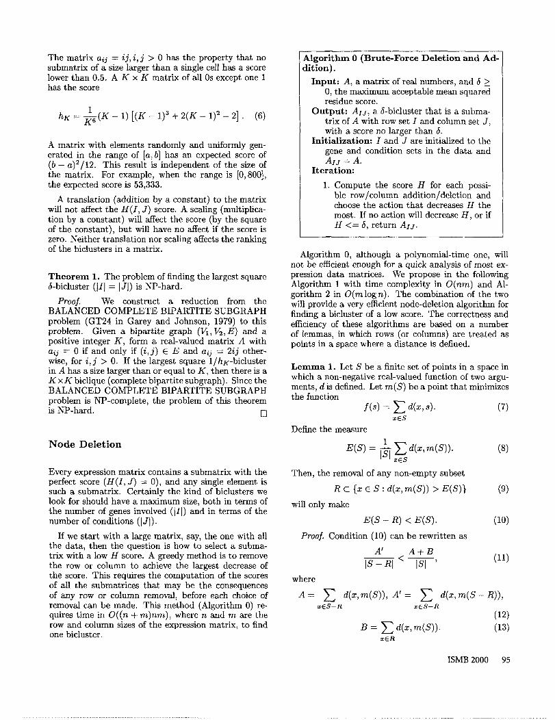
If we start with a large matrix, say, the one with allthe data, then the question is how to select a subma-trix with a low H score. A greedy method is to removethe row or column to achieve the largest decrease ofthe score. This requires the computation of the scoresof all the submatrices that may be the consequencesof any row or column removal, before each choice ofremoval can be made. This method (Algorithm 0) re-quires time in O((n + m)nm), where n and m are therow and column sizes of the expression matrix, to findone bicluster.

Algorithm 0 (Brute-Force Deletion and Ad-dition).

Input: A, a matrix of real numbers, and 5 >0, the maximum acceptable mean squaredresidue score.

Output: Axj, a 5-bicluster that is a subma-trix of A with row set I and column set J,with a score no larger than &

Initialization: I and J are initialized to thegene and condition sets in the data andAH = A.

Iteration:

1. Compute the score H for each possi-ble row/column addition/deletion andchoose the action that decreases H themost. If no action will decrease H, or ifH <= 5, return AIj.

Algorithm 0, although a polynomial-time one, willnot be efficient enough for a quick analysis of most ex-pression data matrices. We propose in the followingAlgorithm 1 with time complexity in O(nm) and Al-gorithm 2 in O(m log n). The combination of the twowill provide a very efficient node-deletion algorithm forfinding a biclnster of a low score. The correctness andefficiency of these algorithms are based on a numberof lemmas, in which rows (or columns) are treated points in a space where a distance is defined.

Lemrna 1. Let S be a finite set of points in a space inwhich a non-negative real-valued function of two argu-ments, d is defined. Let m(S) be a point that minimizesthe function

f(s) = ~ d(x, (7)xES

Define the measure

1E(S) = ~[ ~ d(x, re(S)). (8)

xES

Then, the removal of any non-empty subset

R C {x ¯ S: d(x,m(S)) > E(S)} (9)

will only make

E(S - R) < E(S). (10)

Proof. Condition (10) can be rewritten

A~ A+B

IS- < IS---T’ (11)

where

A= d(x,m(S)), A’ = ~ d(x,m(S xES-R xcS-R

(12)

B = d(x, m(Sl) (13)xER

ISMB 2000 95

The definition of the function rn requires that A’ < A.Thus, a sufficient condition for the inequality (11)

A A+B

Is- < IS---V-’(14)

which is equivalent to

E(S)- A+B B _ ISI < IRI iR--~ ~ d(x, rn(S)). (15)

xER

Clearly, (9) is a sufficient condition for this inequalityand therefore also for (10).

Proo]. Let the points in Lemma 1 be IJI-dimensionalreal-valued vectors and S be the set of vectors bi withcomponents bij = aij - aij for i E I and j 6 J. Thefunction d is defined as

d(bi, bk) = E(bo - bkj)2. (25)jEJ

In this case,1re(S) = Z

i6/

and has the components alj - alj.

(26)

[]

Lenuna 2. Suppose the set removed from S is

R C {x E S: d(x,m(S)) > aE(S)} (16)

with a _> 1. Then the reduction rate of the score E(S)can be characterized as

E(S) - E(S - R) ~ - 1> (17)

E(S) ISl/IRI- 1

When a single point x is removed, the reduction ratehas the bound

d(x, re(S)) - E(S) (18)E(S) - E(S - R) ISl - 1

Proof. Using notation in Lemma I, we have now

A+B B IaE(S) = a--~ < I - IRI E d( x,m(S)). (1 9)

z6R

This leads to

alRIA < (IS] - aIRI)B, (20)

or, equivalently,

ISIA < (ISI - aIRI)(A + (21)

This is the same as

A [SI - a]RI A + BIS - R------~ < IS - RI ISI (22)

Using the inequality A’ < A and the facts that E(S R) = A’/IS - RI and E(S-) (A+B)/ISI, this le ads tothe inequality

E(S - R) < ISI - alRI E(S), (23)Is - RIwhich is (17). Inequality (18) can be derived from (17).

[]

Theorem 2. The set of rows that can be completelyor partially removed with the net effect of decreasingthe score of a bicluster AIj is

{ }a = i e I; IJI jeJ (a~j - a~j azj "~-alJ)2 > H(I, J)

(24)

There is also a similar result for the columns.Lemma 2 acts as a guide on the trade-off between two

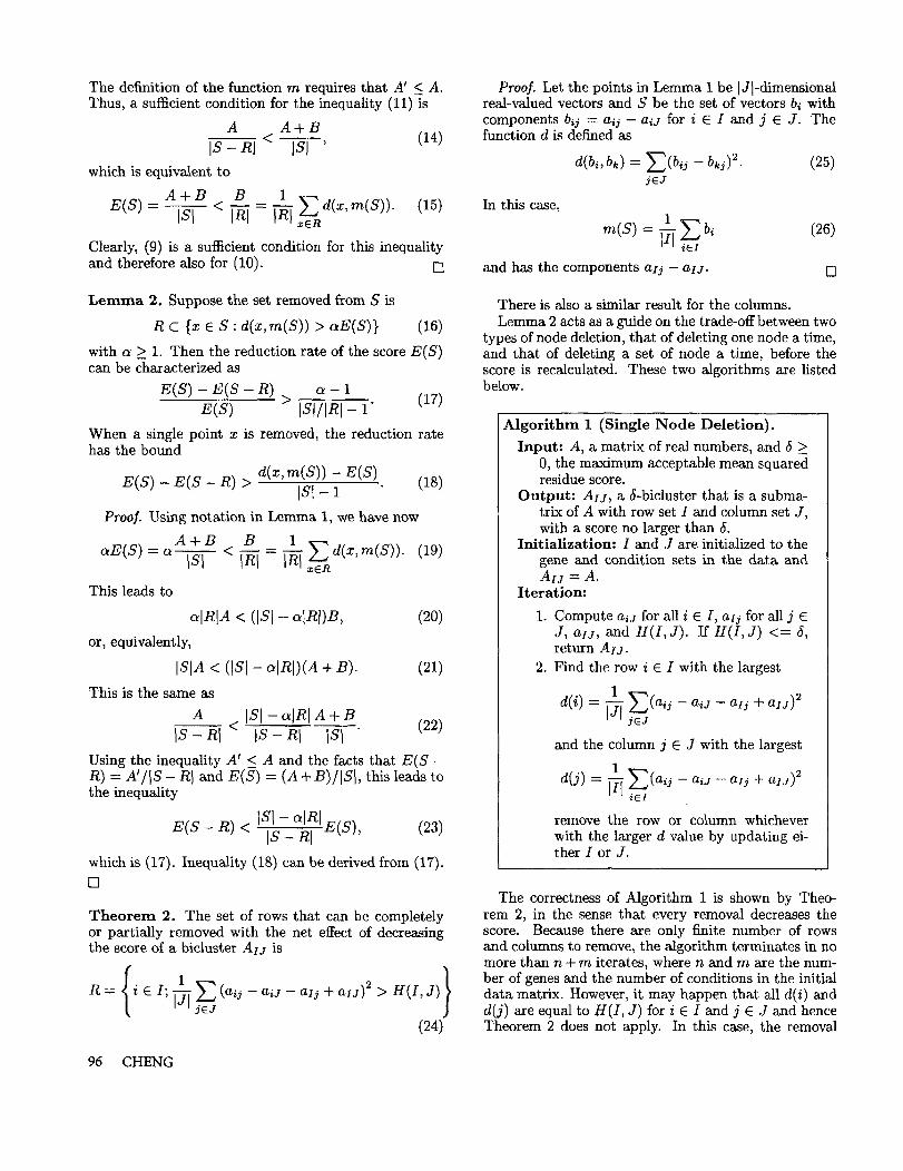
types of node deletion, that of deleting one node a time,and that of deleting a set of node a time, before thescore is recalculated. These two algorithms are listedbelow.

Algorithm 1 (Single Node Deletion).

Input: A, a matrix of real numbers, and 5 >0, the maximum acceptable mean squaredresidue score.

Output: AIj, a 5-bicluster that is a subma-trix of A with row set I and column set J,with a score no larger than &

Initialization: I and J are initialized to thegene and condition sets in the data andA;j = A.

Iteration:

1. Compute aij for all i 6 I, a1j for all j 6J, aij, and H(I, J). If H(I, <= 5,return AIj.

2. Find the row i 6 I with the largest

1E(aij aij + aIj)2d(i) = - - azjj6J

and the column j E J with the largest

1~(aij -- aia -- aIj + alj)2d(j) = -~[ ie’

remove the row or column whicheverwith the larger d value by updating ei-ther I or J.

The correctness of Algorithm 1 is shown by Theo-rem 2, in the sense that every removal decreases thescore. Because there are only finite number of rowsand columns to remove, the algorithm terminates in nomore than n + m iterates, where n and m are the num-ber of genes and the number of conditions in the initialdata matrix. However, it may happen that all d(i) andd(j) are equal to H(I, J) for i 6 I and j E J and henceTheorem 2 does not apply. In this case, the removal

96 CHENG

of one of them may still decrease the score, unless thescore is already zero.

Step 1 in each iterate requires time in O(nm) and complete recalculation of all d values in Step 2 is also anO(nm) effort. The selection of the best row and columncandidates takes O(logn + logrn) time. When the ma-trix is bi-level, specifying "on" and "off" of the genes,the update of various variables after the removal of arow takes only O(m) time and that after the removalof a column only O(n) time. In this case, the algo-rithm can be made very efficient even for whole genomeexpression data, with overall running time in O(nm).But, for non-bi-level matrices, updates are more expen-sive and it is advisable to use the following MultipleNode Deletion before the matrix is reduced to a man-ageable size, when Single Node Deletion is appropriate.

Algorithm 2 (Multiple Node Deletion).Input: A, a matrix of real numbers, 6 > 0,

the maximum acceptable mean squaredresidue score, and a > 1, a threshold formultiple node deletion.

Output: AIj, a 6-bichister that is a subma-trix of A with row set I and column set J,with a score no larger than &

Initialization: I and J are initialized to thegene and condition sets in the data andAH = A.

Iteration:

1. Compute aij for all i 6 I, aO for all j EJ, all, and H(I, J). If H(I, J) <= return AIj.

2. Remove the rows i 6 I with

i > .H(±, J)]g] ~cJ

3. Recompute axj, aij, and H(I, J).4. Remove the columns j E J with

1E(aij-aij-alj+alj) 2 > all(I, J)

III ie*

5. If nothing has been removed in the iter-ate, switch to Algorithm 1.

The correctness of Algorithm 2 is guaranteed byLemma 2. When a is properly selected, the Multi-ple Node Deletion phase of Algorithm 2 (before thecall of Algorithm 1) requires a number of iterates inO(log n + log m), which is usually extremely fast. With-out updating the score after the removal of each node,the matrix may shrink too much and one may miss somelarge 6-biclusters (although later runs of the same algo-rithm may find them). One may also choose aa adaptivea based on the score and size during the iteration.

Node Addition

After node deletion, the resulting &bicluster may notbe maximal, in the sense that some rows and columnsmay be added without increasing the score. Lemma 3and Theorem 3 below mirror Lemma 1 and Theorem 2and provide a guideline for node addition.

Lemma 3. Let S, d, re(S), and E(S) be defined assame as those in Lemma 1. Then, the addition to S ofany non-empty subset

R C {x ~ S: d(x,m(S)) E(S)} (27)

will not increase the score E:

E(S + R) < E(S). (28)

Proof. The condition (28) can be rewritten

A’ A -B,~----r-, (29)

is+hi /i~

where

AE d(x,m(S)), A’= E d(x,m(S+R)),

z6S+R x6S+R

(30)

B = ~ d(x, re(S)). (31)x6R

The definition of the function m requires that A’ _< A.Thus, a sufficient condition for the inequality (29)

A A-B< (321Is + nl IS--7-’

which is equivalent to

E(S)= A-B > B IsI -IRI- [RI ~d(x’m(S)) (33/xER

Clearly, (27) is a sufficient condition for this inequalityand therefore also for (28).

Theorem 3. The set of rows that can be completelyor partially added with the net effect of decreasing thescore of a bicluster AIj is

{1

}R= i~I;-~E(aij-aij-azj+azj) 2 <H(I,J)jEJ

(34)Proof. Similar to the proof of Theorem 2. []

There is also a similar result for the columns.

ISMB 2000 97

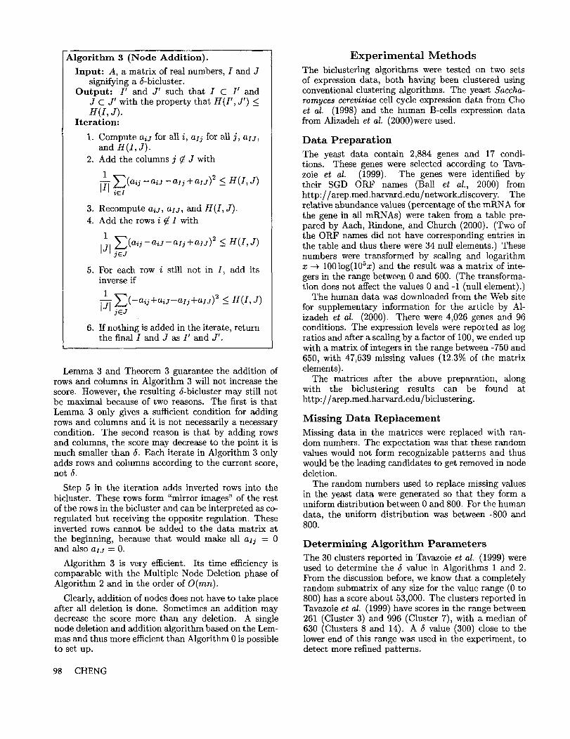
Algorithm 3 (Node Addition).

Input: A, a matrix of real numbers, I and Jsignifying a &bicluster.

Output: I’ and J’ such that I C 11 andJ C J’ with the property that H(I’, J’) H(I, J).

Iteration:

1. Compute aij for all i, alj for all j, at j,and H(I, J).

2. Add the columns j ¢ J with

1 ~-~(a,j -aij -alj +arg)2 < g(I, J)

II] ~ez

3. Recompute a/j, azj, and H(I, J).4. Add the rows i ~ I with

1 ~(a~j-aij-aTj+ajj) 2 <_ H(I, J)IJI jcJ

5. For each row i still not in I, add itsinverse if

1 2 _< H(X, J)’ ’ jEJ

6. If nothing is added in the iterate, returnthe final I and J as I’ and J’.

Lemma 3 and Theorem 3 guarantee the addition ofrows and columns in Algorithm 3 will not increase thescore. However, the resulting 5-bicluster may still notbe maximal because of two reasons. The first is thatLemma 3 only gives a sufficient condition for addingrows and columns and it is not necessarily a necessarycondition. The second reason is that by adding rowsand columns, the score may decrease to the point it ismuch smaller than 5. Each iterate in Algorithm 3 onlyadds rows and columns according to the current score,not 5.

Step 5 in the iteration adds inverted rows into thebicluster. These rows form "mirror images" of the restof the rows in the bicluster and can be interpreted as co-regulated but receiving the opposite regulation. Theseinverted rows cannot be added to the data matrix atthe beginning, because that would make all alj -~ 0and also alj = O.

Algorithm 3 is very efficient. Its time efficiency iscomparable with the Multiple Node Deletion phase ofAlgorithm 2 and in the order of O(mn).

Clearly, addition of nodes does not have to take placeafter all deletion is done. Sometimes an addition maydecrease the score more than any deletion. A singlenode deletion and addition algorithm based on the Lem-mas and thus more efficient than Algorithm 0 is possibleto set up.

98 CHENG

Experimental MethodsThe biclustering algorithms were tested on two setsof expression data, both having been clustered usingconventional clustering algorithms. The yeast Saccha-romyces cerevis~ae cell cycle expression data from Choet al. (1998) and the human B-cells expression datafrom Alizadeh et al. (2000)were used.

Data Preparation

The yeast data contain 2,884 genes and 17 condi-tions. These genes were selected according to Tava-zoie et al. (1999). The genes were identified their SGD ORF names (Ball et al., 2000) fromhttp ://arep.med.harvard.edu/network~iscovery. Therelative abundance values (percentage of the mRNA forthe gene in all mRNAs) were taken from a table pre-pared by Aach, Pdndone, and Church (2000). (Two the ORF names did not have corresponding entries inthe table and thus there were 34 null elements.) Thesenumbers were transformed by scaling and logarithmx -~ 1001og(105x) and the result was a matrix of inte-gers in the range between 0 and 600. (The transforma-tion does not affect the values 0 and -1 (null element).)

The human data was downloaded from the Web sitefor supplementary information for the article by A1-izadeh et al. (2000). There were 4,026 genes and conditions. The expression levels were reported as logratios and after a scaling by a factor of 100, we ended upwith a matrix of integers in the range between -750 and650, with 47,639 missing values (12.3% of the matrixelements).

The matrices after the above preparation, alongwith the biclustering results can be found athttp://arep.med.harvard.edu/biclustering.

Missing Data ReplacementMissing data in the matrices were replaced with ran-dom numbers. The expectation was that these randomvalues would not form recognizable patterns and thuswould be the leading candidates to get removed in nodedeletion.

The random numbers used to replace missing valuesin the yeast data were generated so that they form auniform distribution between 0 and 800. For the humandata, the uniform distribution was between -800 and800.

Determining Algorithm ParametersThe 30 clusters reported in Tavazoie et al. (1999) wereused to determine the fi value in Algorithms 1 and 2.From the discussion before, we know that a completelyrandom submatrix of any size for the value range (0 to800) has a score about 53,000. The clusters reported inTavazoie et al. (1999) have scores in the range between261 (Cluster 3) and 996 (Cluster 7), with a median 630 (Clusters 8 and 14). A ~ value (300) close to lower end of this range was used in the experiment, todetect more refined patterns.

rOWS columns low high peak tail3 6 10 6870 39O 15.5%3 17 30 6600 48O 6.83%

10 6 110 4060 8OO 0.064%10 17 240 3470 87O 0.OO2%30 6 410 2460 96O < 10-6

30 17 480 2310 1040 < I0-~

100 6 630 1720 1020 < 10-6

100 17 700 1630 1080 < 10-6

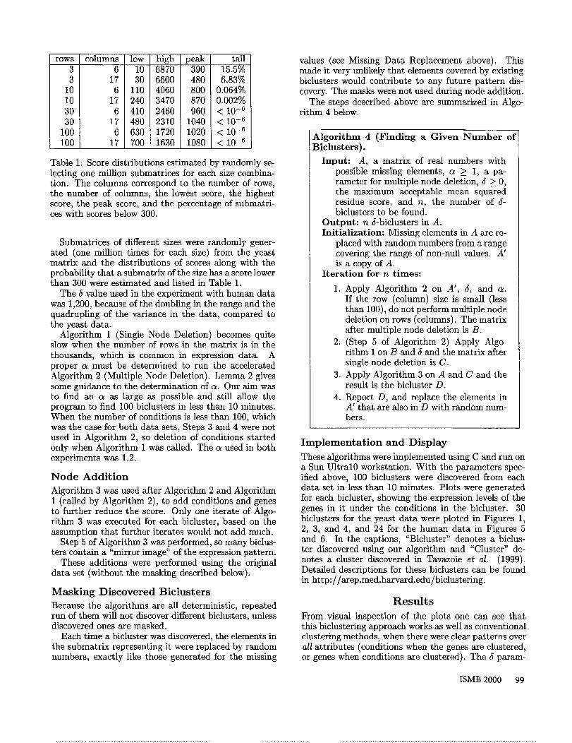
Table 1: Score distributions estimated by randomly se-lecting one million submatrices for each size combina-tion. The columns correspond to the number of rows,the number of columns, the lowest score, the highestscore, the peak score, and the percentage of submatri-ces with scores below 300.

Submatrices of different sizes were randomly gener-ated (one million times for each size) from the yeastmatrix and the distributions of scores along with theprobability that a submatrix of the size has a score lowerthan 300 were estimated and listed in Table 1.

The $ Value used in the experiment with human datawas 1,200, because of the doubling in the range and thequadrupling of the variance in the data, compared tothe yeast data.

Algorithm 1 (Single Node Deletion) becomes quiteslow when the number of rows in the matrix is in thethousands, which is common in expression data. Aproper a must be determined to run the acceleratedAlgorithm 2 (Multiple Node Deletion). Lemma 2 givessome guidance to the determination of a. Our aim wasto find an a as large as possible and still allow theprogram to find 100 biclusters in less than 10 minutes.When the number of conditions is less than 100, whichwas the case for both data sets, Steps 3 and 4 were notused in Algorithm 2, so deletion of conditions startedonly when Algorithm 1 was called. The a used in bothexperiments was 1.2.

Node AdditionAlgorithm 3 was used after Algorithm 2 and Algorithm1 (called by Algorithm 2), to add conditions and genesto further reduce the score. Only one iterate of Algo-rithm 3 was executed for each bicluster, based on theassumption that further iterates would not add much.

Step 5 of Algorithm 3 was performed, so many biclus-ters contain a "mirror image" of the expression pattern.

These additions were performed using the originaldata set (without the masking described below).

Masking Discovered BiclustersBecause the algorithms are all deterministic, repeatedrun of them will not discover different biclusters, unlessdiscovered ones axe masked.

Each time a bicluster was discovered, the elements inthe submatrix representing it were replaced by randomnumbers, exactly like those generated for the missing

values (see Missing Data Replacement above). Thismade it very unlikely that elements covered by existingbiclusters would contribute to any future pattern dis-covery. The masks were not used during node addition.

The steps described above are summarized in Algo-rithm 4 below.

Algorithm 4 (Finding a Given Number ofBiclusters).

Input: A, a matrix of real numbers withpossible missing elements, a > 1, a pa-rameter for multiple node deletion, ~ > 0,the maximum acceptable mean squaredresidue score, and n, the number of ~-biclusters to be found.

Output: n ~-biclusters in A.Initialization: Missing elements in A are re-

placed with random numbers from a rangecovering the range of non-null values. A’is a copy of A.

Iteration for n times:

1. Apply Algorithm 2 on AI, 6, and a.If the row (column) size is small (lessthan 100), do not perform multiple nodedeletion on rows (columns). The matrixafter multiple node deletion is B.

2. (Step 5 of Algorithm 2) Apply Algo-rithm 1 on B and ~ and the matrix aftersingle node deletion is C.

3. Apply Algorithm 3 on A and C and theresult is the bicluster D.

4. Report D, and replace the elements inA’ that are also in D with random num-bers.

Implementation and Display

These algorithms were implemented using C and run ona Sun Ultral0 workstation. With the parameters spec-ified above, 100 biclusters were discovered from eachdata set in less than 10 minutes. Plots were generatedfor each bicluster, showing the expression levels of thegenes in it under the conditions in the bicluster. 30biclusters for the yeast data were ploted in Figures 1,2, 3, and 4, and 24 for the human data in Figures 5and 6. In the captions, "Bicluster" denotes a biclus-ter discovered using our algorithm and "Cluster" de-notes a cluster discovered in Tavazoie et al. (1999).Detailed descriptions for these biclusters can be foundin http://axep.med.haxvaxd.edu/biclustering.

Results

From visual inspection of the plots one can see thatthis biclustering approach works as well as conventionalclustering methods, when there were clear patterns overall attributes (conditions when the genes axe clustered,or genes when conditions are clustered). The ~ param-

ISMB 2000 99

47

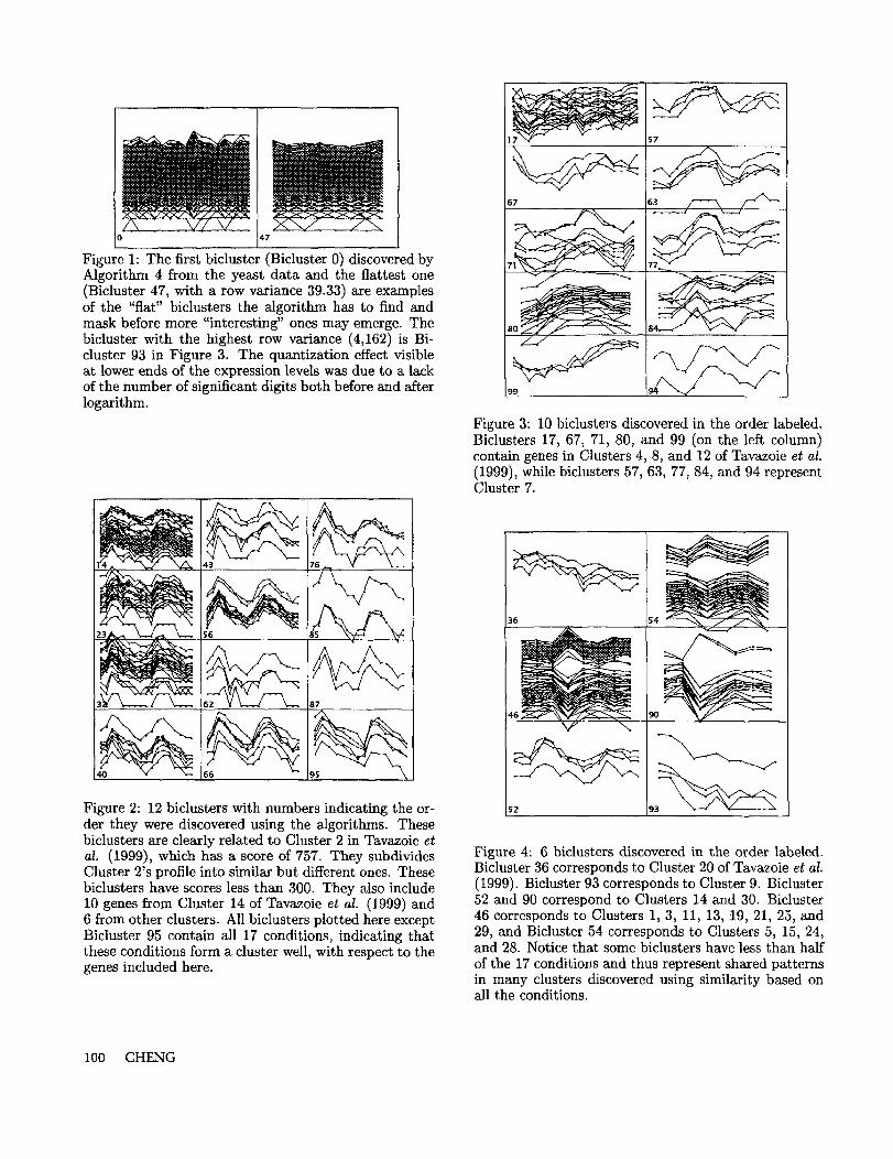
Figure 1: The first bicluster (Bicluster 0) discovered Algorithm 4 from the yeast data and the flattest one(Bicluster 47, with a row variance 39.33) are examplesof the "flat" biclusters the algorithm has to find andmask before more "interesting" ones may emerge. Thebicluster with the highest row variance (4,162) is Bi-cluster 93 in Figure 3. The quantization effect visibleat lower ends of the expression levels was due to a lackof the number of significant digits both before and afterlogarithm.

Figure 2:12 biclusters with numbers indicating the or-der they were discovered using the algorithms. Thesebiclusters are clearly related to Cluster 2 in Tavazoie etal. (1999), which has a score of 757. They subdividesCluster 2’s profile into similar but different ones. Thesebiclusters have scores less than 300. They also include10 genes from Cluster 14 of Tavazoie et al. (1999) and6 from other clusters. All biclusters plotted here exceptBicluster 95 contain all 17 conditions, indicating thatthese conditions form a cluster well, with respect to thegenes included here.

67 63 ~

Figure 3:10 biclusters discovered in the order labeled.Biclusters 17, 67, 71, 80, and 99 (on the left column)contain genes in Clusters 4, 8, and 12 of Tavazoie et al.(1999), while biclusters 57, 63, 77, 84, and 94 representCluster 7.

36

52

Figure 4:6 biclusters discovered in the order labeled.Bicluster 36 corresponds to Cluster 20 of Tavazoie et al.(1999). Bicluster 93 corresponds to Cluster 9. Bicluster52 and 90 correspond to Clusters 14 and 30. Bicluster46 corresponds to Clusters 1, 3, 11, 13, t9, 21, 25, and29, and Bicluster 54 corresponds to Clusters 5, 15, 24,and 28. Notice that some biclusters have less than halfof the 17 conditions and thus represent shared patternsin many clusters discovered using similarity based onall the conditions.

i00 CHENG

eter gives a powerful tool to fine-tune the similarity re-quirements. This explains the correspondence betweenone or more biclusters to each of the better clusters dis-covered in Tavazoie et al. (1999). These includes theclusters associated to the highest scoring motifs (Clus-ters 2, 4, 7, 8, 14, and 30 of Tavazoie et al.). For otherclusters from Tavazoie et al., there were not clear corre-spondence to our biclusters. Instead, Biclusters 46 and54 represent the common features under some of theconditions of these lesser clusters.

Coverage of the BiclustersIn the yeast data experiment, the 100 biclusters covered2,801, or 97.12% of the genes, 100% of the conditions,and 81.47% of the cells in the matrix.

The first 100 biclusters from the human data covered3,687, or 91.58% of the genes, 100% of the conditions,and 36.81% of the cells in the data matrix.

Sub-Categorization of Tavazoie’s Cluster 2Figure 2 shows 12 biclusters containing mostly genesclassified to Cluster 2 in Tavazoie et al.. Each of thesebiclusters clearly represents a variation to the commontheme for Cluster 2. For example, Bicluster 87 con-talns genes with three sharp peaks in expression (CLB6and SPT21). Genes in Bicluster 62 (ERP3, LPP1, andPLM2) showed also three peaks, but the third of these israther fiat. Bicluster 56 shows a clear-cut double-peakpattern with DNA replication genes CDC9, CDC21,POLl2, POL30, RFA1, RFA2, among others. Bicluster66 contains two-peak genes with an even sharper im-age (CDC45, MSH6, RAD27, SWE1, and PDS5). the other hand, Bicluster 14 contains those genes withbarely recognizable double peaks.

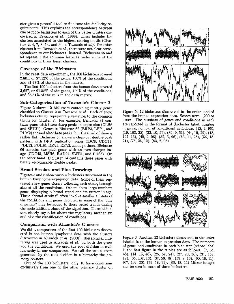
Broad Strokes and Fine DrawingsFigures 5 and 6 show various biclusters discovered in thehuman lymphoma expression data. Some of them rep-resent a few genes closely following each other, throughalmost all the conditions. Others show large numbersgenes displaying a broad trend and its mirror image.These "broad strokes" often involve smaller subsets ofthe conditions and genes depicted in some of the "finedrawings" may be added to these broad trends duringthe node addition phase of the algorithm. These biclus-ters clearly say a lot about the regulatory mechanismand also the classification of conditions.

Comparison with Alizadeh’s ClustersWe did a comparison of the first 100 biclusters discov-ered in the human lymphoma data with the clustersdiscovered in Alizadeh et al. (2000). Hierarchical clus-tering was used in Alizadeh et al. on both the genesand the conditions. We used the root division in eachhierarchy in our comparison. We call the two clustersgenerated by the root division in a hierarchy the pr/-mary clusters.

Out of the 100 biclusters, only 10 have conditionsexclusively from one or the other primary cluster on

.19

I

45

Figure 5:12 biclusters discovered in the order labeledfrom the human expression data. Scores were 1,200 orlower. The numbers of genes and conditions in eachare reported in the format of (bicluster label, numberof genes, number of conditions) as follows. (12, 4, 96),(19, 103, 25), (22, 10, 57), (39, 9, 51), (44, 10, 29), 127, 13), (49, 2, 96), (52, 3, 96), (53, 11, 25), (54, 21), (75, 25, 12), (83, 2,

Figure 6: Another 12 biclusters discovered in the orderlabeled from the human expression data. The numbersof genes and conditions in each bicluster (whose labelis the first figure in the triple) are as follows. (7, 34,48), (14, 15, 46), (25, 57, 24), (27, 23, 30), (31, 17), (35, 102, 13), (37, 59, 18), (59, 8, 19), (60, (67, 102, 20), (79, 18, 11), (86, 18, 11) Mirror can be seen in most of these biclusters.

ISMB 2000 101

conditions. Bicluster 19 in Figure 5 is heavily biasedtowards one primary condition cluster, while Bicluster67 in Figure 6 is heavily biased towards the other.

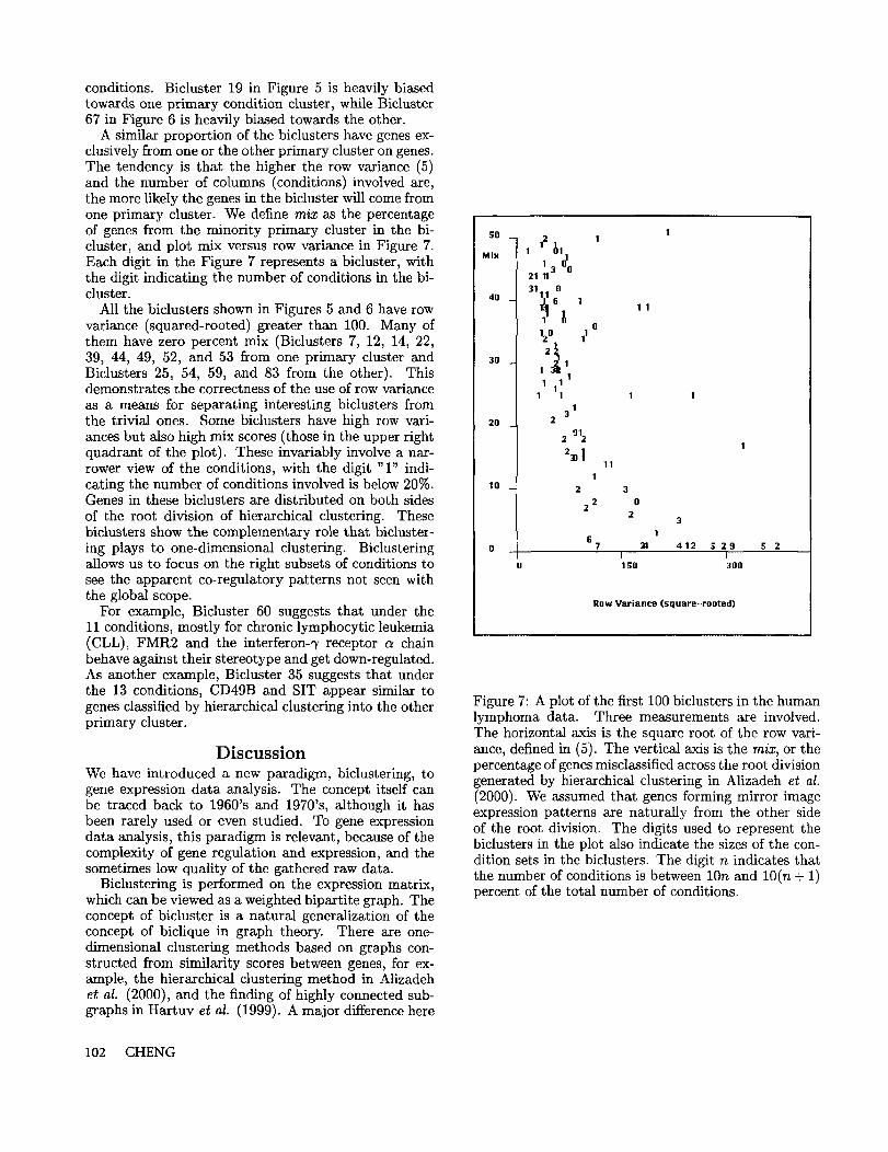
A similar proportion of the biclusters have genes ex-clusively from one or the other primary cluster on genes.The tendency is that the higher the row variance (5)and the number of columns (conditions) involved are,the more likely the genes in the bicluster will come fromone primary cluster. We define m/x as the percentageof genes from the minority primary cluster in the bi-cluster, and plot mix versus row variance in Figure 7.Each digit in the Figure 7 represents a bicluster, withthe digit indicating the number of conditions in the bi-cluster.

All the biclusters shown in Figures 5 and 6 have rowvariance (squared-rooted) greater than 100. Many them have zero percent mix (Biclusters 7, 12, 14, 22,39, 44, 49, 52, and 53 from one primary cluster andBiclusters 25, 54, 59, and 83 from the other). Thisdemonstrates the correctness of the use of row varianceas a means for separating interesting biclusters fromthe trivial ones. Some biclusters have high row vari-ances but also high mix scores (those in the upper rightquadrant of the plot). These invariably involve a nar-rower view of the conditions, with the digit "1" indi-cating the number of conditions involved is below 20%.Genes in these biclusters are distributed on both sidesof the root division of hierarchical clustering. Thesebiclusters show the complementary role that bicluster-ing plays to one-dimensional clustering. Biclusteringallows us to focus on the right subsets of conditions tosee the apparent co-regulatory patterns not seen withthe global scope.

For example, Bicluster 60 suggests that under the11 conditions, mostly for chronic lymphocytic leukemia(CLL), FMR2 and the interferon- 7 receptor a chainbehave against their stereotype and get down-regulated.As another example, Bicluster 35 suggests that underthe 13 conditions, CD49B and SIT appear similar togenes classified by hierarchical clustering into the otherprimary cluster.

DiscussionWe have introduced a new paradigm, biclustering, togene expression data analysis. The concept itself canbe traced back to 1960’s and 1970’s, although it hasbeen rarely used or even studied. To gene expressiondata analysis, this paradigm is relevant, because of thecomplexity of gene regulation and expression, and thesometimes low quality of the gathered raw data.

Biclustering is performed on the expression matrix,which can be viewed as a weighted bipartite graph. Theconcept of bicluster is a natural generalization of theconcept of biclique in graph theory. There are one-dimensional clustering methods based on graphs con-structed from similarity scores between genes, for ex-ample, the hierarchical clustering method in Alizadehet al. (2000), and the finding of highly connected sub-graphs in Hartuv et al. (1999). A major difference here

102 CHENG

50

Mix

4O

3O

2O

I0

1’ 12~1

31 0

012D 11

11 11

13

2

2 9122:B t 11

1

11

1 1

2 32 02 2 3

1£ 7 3:1. 412 S 29 5 2

I" T0 150 300

Row Variance (square-rooted)

Figure 7: A plot of the first 100 biclusters in the humanlymphoma data. Three measurements are involved.The horizontal axis is the square root of the row vari-ance, defined in (5). The vertical axis is the m/x, or thepercentage of genes misclassified across the root divisiongenerated by hierarchical clustering in Alizadeh et al.(2000). We assumed that genes forming mirror imageexpression patterns are naturally from the other sideof the root division. The digits used to represent thebiclusters in the plot also indicate the sizes of the con-dition sets in the biclusters. The digit n indicates thatthe number of conditions is between 10n and 10(n + 1)percent of the total number of conditions.

is that biclustering does not start from or require thecomputation of overall similarity between genes.

The relation between biclustering and clustering issimilar to that between the instance-based paradigmand the model-based paradigm in supervised learning.Instance-based learning (for example, nearest-neighborclassification) views data locally, while model-basedlearning (for example, feed-forward neural networks)finds the globally optimally fitting models.

Biclustering has several obvious advantages over clus-tering. First, biclustering automatically selects genesand conditions with more coherent measurement anddrops those representing random noise. This providesa method for dealing with missing data and corruptedmeasurements.

Secondly, biclustering groups items based on a simi-larity measure that depends on a context, which is bestdefined as a subset of the attributes. It discovers notonly the grouping, but the context as well. And to someextent, these two become inseparable and exchangeable,which is a major difference between biclustering andclustering rows after clustering columns.

Most expression data result from more or less com-plete sets of genes but very small portions of all thepossible conditions. Any similarity measure betweengenes based on the available conditions becomes any-way context-dependent. Clustering genes based on ameasure like this is no more representative than biclus-tering.

Thirdly, biclustering allows rows and columns to beincluded in multiple biclusters, and thus allows one geneor one condition to be identified by more than one func-tion categories. This added flexibility correctly reflectsthe reality in the functionality of genes and overlappingfactors in tissue samples and experiment conditions.

By showing the NP-hardness of the problem, we triedto justify our efficient but greedy algorithms. But thenature of NP-hardness implies that there may be siz-able biclusters with good scores evading the search byany efficient algorithm. Just like most efficient conven-tional clustering algorithms, one can say that the bestbiclusters can be found in most cases, but one cannotsay that it will be found in all the cases.

Acknowledgments

This research was conducted at the Lipper Centerfor Computational Genetics at the Harvard MedicalSchool, while the first author was on academic leavefrom the University of Cincinnati.

References

Aach, J., Rindone, W., and Church, G.M. 2000. Sys-tematic management and analysis of yeast gene ex-pression data. Genome Research in press.

Alizadeh, A.A. et al. 2000. Distinct types of diffuselarge B-cell lymphoma identified by gene expressionprofiling. Nature 403:503-510.

Ball, C.A. et al. 2000. Integrating functional ge-nomic information into the Saccharomyces GenomeDatabase. Nucleic Acids Res. 28:77-80.Cho, R.J. et al. A genome wide transcriptional analysisof the mitotic cell cycle. Mol. Cell 2:65-73.

Garey, M.R., and Johnson, D.S. 1979. Computersand Intractability: A Guide to the Theory of NP-Completeness. San Francisco: Freeman.

Hartigan, J.A. 1972. Direct clustering of a data matrix.JASA 67:123-129.Hartuv, E. et al. 1999. An algorithm for clusteringcDNAs for gene expression analysis. RECOMB ’99,188-197.Johnson, D.S. 1987. The NP-completeness column: anongoing guide. J. Algorithms 8:438-448.

Mirkin, B. 1996. Mathematical Classification andClustering. Dordrecht: Kluwer.

Morgan, J.N. and Sonquist, J.A. 1963. Problems in theanalysis of survey data, and a proposal. JASA 58:415-434.Nan, D.S., Markowsky, G., Woodbury, M.A., andAmos, D.B. 1978. A mathmatical analysis of humanleukocyte antigen serology. Math. Biosci. 40:243-270.Orlin, J. 1977. Containment in graph theory: coveringgraphs with cliques, Nederl. Akad. Wetensch. Indag.Math. 39:211-218.Tavazoie, S., Hughes, J.D., Campbell, M.J., Cho, R.J.,and Church, G.M. 1999. Systematic determination ofgenetic network architecture. Nature Genetics 22:281-285.Yannakakis, M. 1981. Node deletion problems on bi-partite graphs. SIAM J. Comput. 10:310-327.

ISMB 2000 103