beyond inventory management: the bullwhip effect and the

Beyond Inventory Management:The Bullwhip Effect and the Great Moderation

Michael McMahonUniversity of Warwick

CEPR, CfM, CAGE, CAMA

Boromeus Wanengkirtyo ∗

University of Warwick

22 December 2015

Abstract

We resurrect the question of whether improved business practices con-tributed to increased macroeconomic stability since the 1980s (the so-calledGreat Moderation). While previous studies on the issue are limited to exam-ining inventory management, we analyse the role of better supply chain man-agement on enhancing firms’ ability to coordinate their production. By inves-tigating ordering and backordering behaviour in the durables manufacturingsector, we find that the improved business practices have significantly damp-ened order volatility to the sector (the ‘bullwhip effect’), by around 40-50%.Using the stylised fact that the durables manufacturing sector is responsiblefor half of the overall Great Moderation, we determine that the contribution ofbetter business practices is quantitatively significant, at 20-25% of the overallGreat Moderation.

JEL Classifications: E32, L60

Keywords: Economic Fluctuations, Inventory, Durable Good, Supply Chain.

∗We are grateful for helpful comments from George Alessandria, Mike Clements, Thomas Lubik,Dennis Novy, Giorgio Primiceri, Irfan Qureshi, Thijs van Rens and Mike Waterson, as well as partic-ipants at the Money, Macro and Finance 2013 conference and American Economic Association 2014ISIR session. Boromeus Wanengkirtyo acknowledges the ESRC for research funding.

1. Introduction

Despite the Great Recession, understanding the causes of the period of prolonged

macroeconomic stability that preceded it (known as the Great Moderation) re-

main important. This is because if that period was driven mostly by good luck,

as suggested in Stock and Watson (2003), Ahmed, Levin, and Wilson (2004), Kim,

Nelson, and Piger (2004) and Herrera and Pesavento (2005), then there is no reason

to expect such stability to resume. Studies that estimate the changes in the reac-

tion function of the Federal Reserve like Clarida, Galí, and Gertler (2000), Cogley

and Sargent (2001), Orphanides (2004) and Boivin and Giannoni (2006) are propo-

nents that better monetary policy was a main driver. Stability induced by better

monetary policy is more likely to be continued.

New business practices, often taken to mean better inventory management tech-

niques, is a third suggested cause for the Great Moderation and are also likely to

be a more persistant driver of lower volatility. McConnell and Perez-Quiros (2000),

Blanchard and Simon (2001) and Kahn, McConnell, and Perez-Quiros (2002) sug-

gested there was a substantial role for inventory management. However others,

such as Stock and Watson (2003), consider the role for inventory management

and dismiss it. McCarthy and Zakrajšek (2007) using a VAR analysis of the Great

Moderation concluded that inventory management played, at most, a supporting

role. The reason earlier papers tend to dismiss a role for new business practices is

related to the focus on inventories and is summed up nicely by Taylor (2013):

“Firms cut inventories when sales weaken and rebuild inventories when sales

strengthen. Better inventory control could thus explain the improved stabil-

ity. But this explanation also had problems. When one looked at final sales –

GDP less inventories – one saw the same amount of improvement in economic

stability.”

Our main contribution in this paper is to extend the concept of business prac-

tices to include supply chain management and backordering behaviour in addition

1

to inventory management. Importantly, we will argue that changes in business

practices can endogenously dampen sales volatility. As such, the reduction in

sales volatility is not sufficient to reject a central role for new business practices.

Davis and Kahn (2008) considered the potential contribution of supply chain man-

agement in the Great Moderation, but leaves how it connects with sales volatility

as an open question.

We focus on the durables manufacturing sector. We do this for a number of

reasons. First, despite accounting for only about 20% of GDP, durables production

is one of the biggest contributors to output volatility.1 Second, it is also one of the

biggest contributors to output moderation as a result of a large fall in within-

sector volatility (Stock and Watson, 2003); a back-of-the-envelope calculation from

the results in Stock and Watson (2003) suggests that it accounts for around half

of the overall Great Moderation (see Table 7 in the appendix). Third, McConnell

and Perez-Quiros (2000) and Davis and Kahn (2008) show the timing of durables

output volatility falls, impeccably matches the observed break in GDP volatility.

Finally, manufacturing industries are placed upstream of the supply chain, and

therefore, has the most to benefit from the new business practices; for example,

backorder books are sizeable in durables manufacturing.

We make two specific empirical contributions. First, motivated by the finding of

Zarnowitz (1962) that firms respond to demand shocks by accumulation/depletion

of backorders first (changing lead times), we document how the Great Moderation

was not just a period of lower inventory investment volatility but can also be char-

acterised by quicker delivery, shorter lead times and reduced use of backordering

in the durable goods manufacturing sector. To explore what these developments

mean for the analysis of the effects of new business practices, rather than focus on

the production identity that states production (Y) is equal to the sum of sales (S)

and inventory investment (∆I), we further disaggregate sales into its components

1About 2-2.5 times more volatile than non-durables, and 6-10 times more than services (Table 7in Stock and Watson (2003)).

2

of new orders O and adjustments to backorders ∆U:

Y = S +∆I

= (O− ∆U) +∆I.(1)

We find that reduced volatility of new orders accounts for the majority of sales

and production volatility falls. Given that the previous literature claims that the

decline in sales volatility is most likely driven by background macro factors (good

luck or good policy), a similar argument would likely be adopted to explain de-

clining new order volatility. They would consider this as similar evidence that we

need to look at alternative explanations to new business practices. However, given

that most orders in the manufacturing sector are placed by intermediate goods

producers, rather than consumers, supply chain management can be an important

determinant of order volatility. We argue that improved business practices can

endogenously dampen order volatility; upstream suppliers meeting new orders

consistently more quickly can give rise to a reduction in the volatility of sales.

This is unlike the analysis in standard macroeconomic models of inventories.

The second empirical contribution is to show that improved business practices

contributed substantially more to the Great Moderation than previously thought.

While still not the dominant contributor, this channel can account for 20-25% of

the output volatility declines. This finding comes from our application of the em-

pirical approach of McCarthy and Zakrajšek (2007) (MZ hereafter) to our broader

concept of business practices in the durabless manufacturing sector. We estimate a

separate structural VAR for the pre-1979 (High Volatility, HV) and post-1984 (Low

Volatility, LV) period. Using forecast standard errors as a measure of volatility, we

ask the question if volatility reductions emanate from luck and macroeconomic

changes, better business practices (identified as sector-level structural changes), or

a combination of both.

Counterfactuals between the two SVARs suggest that sector-level structural changes

have contributed to approximately half of the fall of new orders volatility. We

3

interpret this as the result of a dampening of the ‘bullwhip effect’ (Lee, Padmanab-

han, and Whang, 2004)– the well-documented phenomenon where demand shocks

from downstream consumers are amplified through the supply chain to upstream

producers. New business practices, such as the adoption of Electronic Data In-

terchange ICT systems which led to better communication along supply chains,

would diminish the amplification of new orders volatility and stabilise production.

We also find evidence of changes in backordering behaviour. The successful

adoption of lean production and just-in-time techniques reduces the need for back-

orders to smooth out demand shocks and, as a consequence, delivery times would

lower and more consistent. Finally, we find that implied inventory volatility (as a

proportion of inventory stocks) in the durables sector actually increases.2 This is

suggestive of the adoption of flexible production processes (as predicted by most

macroeconomic models of inventories and production flexibility such as Alessan-

dria, Kaboski, and Midrigan (2013) and McMahon (2012).

The rest of the paper is organised as follows. Section 2 describes the data used

and establishes some motivating stylised facts. Section 3 details the bullwhip effect

that the empirical evidence we present in this paper supports. Section 4 introduces

the structural vector autoregression, and the counterfactual methodology. Section

5 analyses the results and implications for the role of business practices on the

Great Moderation. Section 6 concludes.

2. New Business Practices: Technologies and Stylised Facts

Anyone reading the management and operations research literature will be left in

no doubt that business practices have evolved a great deal since the 1960s. New

technologies allow firms much greater control over their production, sales and dis-

tribution processes. In this section we first review the broad types of technological

improvements that many practicitioners consider as driving forces for improved

2The MZ result that inventory volatility has fallen holds in the non-durables manufacturingSVAR (reported in the appendix). This indicates that particular result was driven by the muchlarger non-durables sector.

4

management of inventories and distribution. We then examine developments in

the durables manufacturing sector to see how production and distribution, back-

ordering, and inventories (disaggregated into stages of production – materials and

supplies, work-in-process and finished goods inventories) evolved before and dur-

ing the Great Moderation.

Our analysis uses industry-level monthly data is from the United States Census

Bureau. The historic time series for Manufacturers Shipments, Inventories & Orders

covers January 1967 to December 1996. All variables are in current dollars (by

net selling values) and seasonally adjusted. To deflate the variables, we use the

implicit sales price deflators from the Bureau of Economic Analysis.3

2.1. Back-ordering and the Bullwhip Effect

Before we turn to an analysis of the new technologies that have affected (in partic-

ular) the manufacturing sector, we describe two important related characteristics

of manufacturing supply chains. We believe that these characteristics are key to

understanding the Great Moderation but are generally under-researched areas of

macroeconomics.

The first concept is backordering. Zarnowitz (1962) documented that firms re-

spond to demand shocks by accumulation/depletion of backorders first (chang-

ing lead times), then adjusting inventories, and eventually changing production

and/or prices. The role of backorders is particularly relevant in durables manu-

facturing where backorder books are sizeable and backorder adjustments account

for substantial variance of production and sales growth.

The second concept is the bullwhip effect. This supply-chain phenomenon,

dating back to Forrester (1961), is well-documented in the management science

literature. It captures the situation whereby demand shocks from downstream

consumers are amplified through the supply chain to upstream producers. Lee,

3Deflating the nominal variables using these price deflators makes the implicit assumption thatthe intra-sector composition of inventory investment, backorders and new orders are the same assales.

5

Padmanabhan, and Whang (2004) group the causes into four categories: demand

signal processing, shortages and rationing gaming, order batching, and price vari-

ations. Let us look in more detail at how each of these causes to see how they give

rise to extra volatility in the manufacturing sector (and to make clear how some

are directly related to the use of backordering).

Firstly, demand signal processing results from the need of producers to forecast

future demand by using their immediate customer’s orders. If there are lead-times

in production and delivery of raw materials, positive autocorrelation of demand,

and each member of the supply chain processes the order signals from below,

shocks are amplified as they go upwards through the supply chain.

Secondly, shortages are a period of more extensive use of backordering. This

contributes to the bullwhip effect when customers attempt to manipulate their

supplier’s rationing. If the producer fulfils orders of a good that is short in supply

on the basis of order size in proportion to total orders, customers will place extra

‘phantom orders’ in order to get more of the good. When the supply shortage

eventually clears, they cancel their phantom orders and, thus, the producer sees

amplified fluctuations in their order book.

Thirdly, order batching by downstream firms creates volatility of order inflows

for the manufacturing. This occurs when a firm’s own demand comes in, depleting

inventory, but they may not place an order immediately with its supplier. This may

be due to the fact that material requirement planning (MRP) systems are run only

monthly, or due to firms attempting to get economies of scale from delivery and

order processing costs (including management time to process the order).

Finally, price variations may lead a customer to attempt to build inventory (high

orders) during times of low prices, and the opposite when prices are high. This

leads to large, irregular orders. Such periods of low nad high prices may follow

from over-reactive production which results in periods of large excess supply and

periods of severely limited supply. This means price variation is both a result of,

and contributor to, the bullwhip phenomenon.

6

2.2. New Technologies Affecting Durables Manufacturing

Improvements of supply chain management are based on the introduction of ICT-

based systems and lean production. To understand why these might have a sta-

bilising effect on the production of durables, we now discuss some of the main

developments and link them to our two important channels. We stress three broad

developments (which are also related):

1. Electronic Data Interchanges (EDIs)

2. Vendor Management Inventory (VMI)

3. Just-in-Time Production (JIT)

The adoption of ICT systems by manufacturers, and all along the supply chain,

allowed for widespread use of EDI. That is, computers from one firm in the supply

chain could send information to another firm in a standardized format and with

little need for human intervention. This has led to better communication, and

vitally better information, along supply chains.

VMI makes the (upstream) manufacturer responsible for maintaining appropri-

ate inventory levels at downstream links in the supply chain (such as a whole-

saler). The downstream firm agrees to provide detailed and timely information

on sales and inventory levels. The manufacturer can then optimally fulfill orders

across each of the (potentially many) downstream firms.

JIT, or lean manufacturing, is an approach to manufacturing which originated

in Japan and is associated with Toyota. It made its way to the West in 1977. It

involves reduced waste and shorter lead times in production which in turn facili-

tates greater flexibility in the manufacturing. A simplistic view of flexible manu-

facturing is that it leads to more volatile production. However, flexibility to meet

demands in a more responsive fashion (for example by changing production from

focusd on one product to focused on another) may actually give rise to greater

stability. As we will argue, reduced and more consistent lead times by the manu-

7

facturer may endogenously change ordering behaviour by downstream firms.

These three new business practices are inter-related. For example, while VMI

was an impetus for widespread adoption of EDI (in exchange for information

the downstream firm no longer had to manage the inventory), it is also the case

that VMI could only work because of EDI. Causality similarly runs both ways

when we consider JIT and EDI, or JIT and VMI; VMI/EDI led to faster delivery

response times, and computerised flow production allowed firms to more easily

adjust production.

2.3. The Evolution of Durables Manufacturing: Some Stylized Facts

Regardless of the extent to which these new practices caused each other, it should

be clear that they, at least potentially, could give rise to profound effects on the use

of backordering and the bullwhip effect. In this subsection, we establish some styl-

ized facts on the evolution of key variables in the durables manufacturing sector

over time and particularly in the Great Moderation. These facts can shed light on

the aforementioned channels by demonstrating the effects of the adoption of im-

proved supply chain management techniques and flexible production processes.

These stylised facts can be grouped into the following:

1. Reductions in production materials lead times

2. Reductions in lead time volatility

3. Reductions in backorders-sales ratios

4. Reductions in inventories-sales ratios

Since firms respond faster by adjusting production, delivery times became lower

and more consistent. Figure 1 shows that there have been large falls in production

materials delivery lead times. There was a sharp reduction in lead times between

pre-1980 and post-1984 (mean of 72 and 49 days, respectively). These declines

began in the early-1980s and coincide with a rapid increase in firms achieving

JIT ordering; Figure 2 shows that the proportion of manufacturing firms with JIT

8

ordering (defined as receiving orders in less than five days) more than tripled from

before the 1980s to the Great Moderation period.

Avg. HV = 77 days

Avg. LV = 49 days60

90

120

1970 1975 1980 1985 1990 1995Time

Manufacturing Production Materials Average Lead Times (in days)

Figure 1: Average Manufacturing Production Materials Lead Times

Notes: Insitute for Supply Management data. Shaded areas are NBER-dated recessions.

9

Avg. HV = 6 %

Avg. LV = 21 %

0

10

20

1960 1970 1980 1990 2000 2010Time

Percentage of Manufacturing Firms with JIT Ordering

Figure 2: Percentage of Manufacturing Firms with Just-in-Time ordering

Notes: JIT defined as receiving orders in less than five days. Shaded areas are NBER-dated recessions.

As we will argue below, it is not only the first moment that affects ordering

behaviour, but also the variance of lead times. This relates to the reduction in

the backorder adjustment margin and consistency of delivery times. As a proxy

for leadtime disruptions, we calculate rolling volatilities of the Institute for Sup-

ply Management’s Manufacturing Supplier Deliveries Index.4 We use this index,

rather than raw delivery times, as it is calculated like the Purchasing Managers’

Index – it emphasises changes to delivery times, which is the crucial factor in de-

termining disruptions to production scheduling. Figure 3 shows a sharp decline

in volatility from the early 1980s. Increased delivery consistency allows manufac-

turers to improve production scheduling, and implement just-in-time practices to

respond to demand shocks faster.

4The volatilities are calculated by the Qn estimator of scale.

10

10

20

1950 1960 1970 1980 1990 2000 2010

Time

ISM Manufacturing Delivery Index Volatility

Figure 3: Volatility of ISM Manufacturing Deliveries Index.

Notes: Authors’ own calculations. Calculated as the 36-month Backward-Lookingrolling standard deviation of the ISM Manufacturing Deliveries Index.

JIT allows producers to respond faster to demand fluctuations and so allows

firms to reduce backorder books. There is also less need to use backordering

because, through VMI, the manufacturer can essentially reduce desired inventory

across downstream firms while they adjust production smoothly. We see there is a

large fall in durables sector backorders (relative to sales) in the early 1980s (figure

4).5 However, this decline occurred only gradually and is not as stark as the

previous stylized facts. This might be expected given it is a stock variable and so

may take somewhat longer to adjust. It is worth noting that while the backorder-

book size has declined, the higher frequency volatility remains relatively high.

This is important as it is the change in backorder books, and not the size of them,

that affects production volatility.

5We exclude the Transportation sector due to its special characteristic of extremely long leadtimes, which would not be informative on the state of supply chain management. The total durablesmanufacturing and disaggregated data is available in the appendices.

11

2.0

2.5

3.0

3.5

1970 1975 1980 1985 1990 1995Time

Backorders−Sales Ratios for Durables except Transportation

Figure 4: Backorders to Shipments Ratio (excluding Transportation sector)

Notes: We exclude the Transportation sector due to its special characteristic of extremelylong lead times, which would not be informative on the state of supply chain manage-ment. Shaded areas are NBER-dated recessions.

Finally we turn to the evolution of inventories – the focus of most of the pre-

vious literature. Inventories-sales ratios for the durables sector have also fallen

since the early 1980s (figure 5). This was driven mostly by materials and supplies

inventories first in the late 1970s (and to a lesser extent, final goods inventories). It

was only in the 1990s that holdings of work-in-progress inventories fell strongly.

This suggests steady improvements in inventory control but perhaps not as starkly

occurring at the time associated with the start of the Great Moderation.

12

0.4

0.6

0.8

1.0

1970 1975 1980 1985 1990 1995Time

FG M&S WIP

Inventories−Sales Ratios for Durables

Figure 5: Inventories to Shipments Ratio

Notes: We exclude the Transportation sector due to its special characteristic of extremelylong lead times, which would not be informative on the state of supply chain manage-ment. Shaded areas are NBER-dated recessions.

3. Analysis of Volatility: Role of New Business Practices

The previous section presents evidence of the effects of new business practices in

durables manufacturing. Importantly given the exisiting literature, the evidence

pointed to effects outside of simply changes in how inventories are managed. We

also suggest that these changes should affect volatility. We therefore now turn our

attention to the behaviour of volatility in the durables manufacturing industry.

We will focus on the comparison of two twelve-year periods to try to capture

the ‘steady state’ volatility in each period. The first period covers January 1967

to December 1978 and we call it the High Volatility (HV) period (as MZ do).

The second is the Low Volatility (LV) period covering January 1984 to December

1996.6 This split follows MZ and allows for a transition period from 1979 to 1983

during which the exceptional volatility of the Volcker disinflation and extensive6We stop in December 1996 to ensure comparable data across the HV and LV periods.

13

manufacturing restructuring may contaminate the results. (Some of the figures we

presented of inventories and backorder behaviour clearly show that this interval

was indeed a transition period.)

3.1. Volatility Decomposition

In this subsection we document a volatility decomposition of durable manufac-

turing production volatility. We use (1) applied to quarterly growth rates (mean-

ing that the RHS terms are quarterly growth contributions) and then examine

the following volatility decomposition (where V(x) denotes the variance of x and

Cov(x,z) denotes the covariance of x and z):

V(Y) = (V(O) + V(∆U)− 2Cov(O, ∆U)) + V(∆I) + 2Cov(S, ∆I). (2)

In table 1 we present this decomposition in the form of standard deviations for

the HV and LV periods. The advantage of using standard deviations is that it

allows us to express everything in terms of five core drivng parameters:

1. σ∆I ≡√

V(∆I) is the standard deviation of the change in inventories

2. σO ≡√

V(O) is the standard deviation of new orders

3. σ∆U ≡√

V(∆U) is the standard deviation of the change in backorders

4. ρS,∆I is the correlation coefficient between S and ∆I

5. ρO,∆U is the correlation coefficient between O and ∆U

The other terms of equation (2) can be expressed as functions of these five pa-

rameters. For example, Cov(O, ∆U) = ρO,∆U(σO)(σ∆U) and V(S) = (σ2O + σ2

∆U −2ρO,∆U(σO)(σ∆U).

14

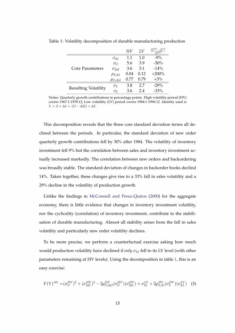
Table 1: Volatility decomposition of durable manufacturing production

HV LV XHV−XLV

XHV

Core Parameters

σ∆I 1.1 1.0 -9%σO 5.6 3.9 -30%

σ∆U 3.6 3.1 -14%ρS,∆I 0.04 0.12 +200%ρO,∆U 0.77 0.79 +3%

Resulting VolatilityσY 3.8 2.7 -29%σS 3.6 2.4 -33%

Notes: Quarterly growth contributions in percentage points. High volatility period (HV)covers 1967:1-1978:12; Low volatility (LV) period covers 1984:1-1996:12. Identity used isY = S + ∆I = (O− ∆U) + ∆I.

This decomposition reveals that the three core standard deviation terms all de-

clined between the periods. In particular, the standard deviation of new order

quarterly growth contributions fell by 30% after 1984. The volatility of inventory

investment fell 9% but the correlation between sales and inventory investment ac-

tually increased markedly. The correlation between new orders and backordering

was broadly stable. The standard deviation of changes in backorder books declind

14%. Taken together, these changes give rise to a 33% fall in sales volatility and a

29% decline in the volatility of production growth.

Unlike the findings in McConnell and Perez-Quiros (2000) for the aggregate

economy, there is little evidence that changes in inventory investment volatility,

nor the cyclicality (correlation) of inventory investment, contribute to the stabili-

sation of durable manufacturing. Almost all stability arises from the fall in sales

volatility and particularly new order volatility declines.

To be more precise, we perform a counterfactual exercise asking how much

would production volatility have declined if only σ∆I fell to its LV level (with other

parameters remaining at HV levels). Using the decomposition in table 1, this is an

easy exercise:

V(Y)Alt =(σHVO )2 + (σHV

∆U )2 − 2ρHVO,∆U(σ

HVO )(σHV

∆U ) + σLV∆I + 2ρHV

S,∆I(σHVS )(σLV

∆I ) (3)

15

We then repeat the exercise changing the appropriate parameters to ascertain what

would have happened to production volatility if only σO or σ∆U changed.

If only the inventory investment term, changed production volatility would have

declined a very small amount. In fact, the decline makes up less than 3% of the

actual decline in volatility that took place. By changing new orders volatility,

the implied production volatility makes up around 90% of the actual decline we

observe. In contrast, changing backorders volatility actually increases volatility

slightly. This is because the fall in backorder variance does not compensate enough

for the less-negative covariance term.

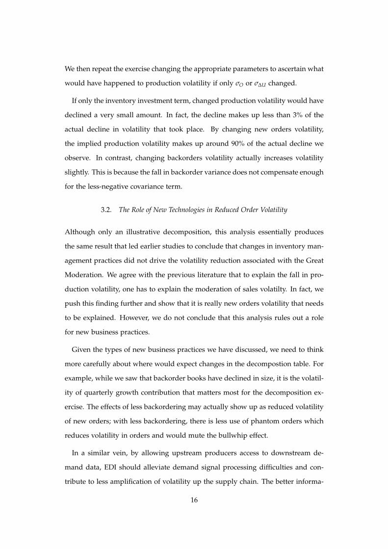
3.2. The Role of New Technologies in Reduced Order Volatility

Although only an illustrative decomposition, this analysis essentially produces

the same result that led earlier studies to conclude that changes in inventory man-

agement practices did not drive the volatility reduction associated with the Great

Moderation. We agree with the previous literature that to explain the fall in pro-

duction volatility, one has to explain the moderation of sales volatilty. In fact, we

push this finding further and show that it is really new orders volatility that needs

to be explained. However, we do not conclude that this analysis rules out a role

for new business practices.

Given the types of new business practices we have discussed, we need to think

more carefully about where would expect changes in the decompostion table. For

example, while we saw that backorder books have declined in size, it is the volatil-

ity of quarterly growth contribution that matters most for the decomposition ex-

ercise. The effects of less backordering may actually show up as reduced volatility

of new orders; with less backordering, there is less use of phantom orders which

reduces volatility in orders and would mute the bullwhip effect.

In a similar vein, by allowing upstream producers access to downstream de-

mand data, EDI should alleviate demand signal processing difficulties and con-

tribute to less amplification of volatility up the supply chain. The better informa-

16

tion means that manufacturers are less likely to be surprised by changes in orders,

or can better identify purely transitory movements in downstream demand. JIT

allows producers to respond faster to demand fluctuations and therefore interme-

diate goods producers know they will receive extra orders speedily if they them-

selves experience a demand shock. In response to shorter and more consistent

delivery times, intermediate goods producers stop making large, irregular orders

when lead times are low (previously necessary to build up materials inventories

and avoid costly materials stockouts).

We believe that new business practices can endogenously change the volatility

orders; other researchers have interpreted orders or sales as exogenous processes

(to new business practices). Our interpretation leaves open a clearer role for new

business practices, and in particular the dimensions of supply chain management

discussed above.

Such endogenous demand processes are not standard in typical models of busi-

ness cycles and inventories. For example in the RBC model of Alessandria, Ka-

boski, and Midrigan (2013), retailers buy an input subject to both idiosyncratic

demand uncertainty and re-order uncertainty. A new business practice that re-

duces the inventory-sales ratio 15% (a figure from Khan and Thomas (2007)) would

increase output volatility slightly. Similarly, in McMahon (2012), more flexible dis-

tribution technology leads to greater (not lesser) volatility of production for given

other exogenous processes.

However, in the operations research literature such endogeneity is more com-

mon. In fact, in that literature the dependence of new order volatility on back-

ordering behaviour and lead times variability is well-established. For example,

Song and Zipkin (1996) shows that consistent lead times on a firms own orders

affects inventory and ordering behaviour. Song, Zhang, Hou, and Wang (2010)

show that in response to stochastically shorter lead times, customers will opti-

mally reduce the amount of safety inventory that they hold and reduce the size of

orders. The response to less-variable lead times is, however, ambiguous.

17

Of course, the overall effect of new business practices is an empirical question.

Our decomposition, while interesting, does not allow us to conclude that there was

or was not a crucial role for new business practices. However it does convince us

that any role should manifest itself through reduced new orders volatility onto

increased stability of durable goods production. Of course, nothing precludes the

macroeconomic factors from driving these changes; reduced downstream aggre-

gate demand volatility as a result of good luck or good policy could also lead to

lower upstream order volatility. We have merely argued that new business prac-

tices may be an adequate explanation.

We now want to push our analysis further, and especially to establish more

clearly the direction of causality. To disentangle between the three effects and

establish causality, we now adopt a multivariate approach. This VAR analysis

will allow us, subject to our identification scheme, to formalise the links between

aggregate and the sector-level variables.

4. Separating Out Business Practices and Macro Effects

This section explores new order, inventory and backorder dynamics in the durables

manufacturing sector, within a structural VAR framework. Building on the method-

ology of MZ, we examine possible structural changes in the economy by esti-

mating separate SVAR models for the pre-1979 (High Volatility) period and the

post-1984 (Low Volatility) period. We then apply a counterfactuals decomposition

methodology that follows Stock and Watson (2003) as well as Simon (2001), to

analyse the structural contribution of each variable to overall forecast error vari-

ance. In this section we will make clear the specific approach we use and the

identification assumptions we make.

18

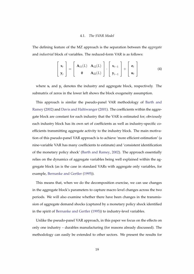
4.1. The SVAR Model

The defining feature of the MZ approach is the separation between the aggregate

and industrial block of variables. The reduced-form VAR is as follows:

xt

yt

=

A11(L) A12(L)

0 A22(L)

·

xt−1

yt−1

+

et

ut

(4)

where xt and yt denotes the industry and aggregate block, respectively. The

submatrix of zeros in the lower left shows the block exogeneity assumption.

This approach is similar the pseudo-panel VAR methodology of Barth and

Ramey (2002) and Davis and Haltiwanger (2001). The coefficients within the aggre-

gate block are constant for each industry that the VAR is estimated for; obviously

each industry block has its own set of coefficients as well as industry-specific co-

efficients transmitting aggregate activity to the industry block. The main motiva-

tion of this pseudo-panel VAR approach is to achieve ‘more efficient estimation’ (a

nine-variable VAR has many coefficients to estimate) and ‘consistent identification

of the monetary policy shock’ (Barth and Ramey, 2002). The approach essentially

relies on the dynamics of aggregate variables being well explained within the ag-

gregate block (as is the case in standard VARs with aggregate only variables, for

example, Bernanke and Gertler (1995)).

This means that, when we do the decomposition exercise, we can use changes

in the aggregate block’s parameters to capture macro level changes across the two

periods. We will also examine whether there have been changes in the transmis-

sion of aggregate demand shocks (captured by a monetary policy shock identified

in the spirit of Bernanke and Gertler (1995)) to industry-level variables.

Unlike the pseudo-panel VAR approach, in this paper we focus on the effects on

only one industry – durables manufacturing (for reasons already discussed). The

methodology can easily be extended to other sectors. We present the results for

19

the non-durables manufacturing sector in the appendix.7

Relative to MZ, we follow our earlier analysis and include extra variables in

our industry block: xt = [ot ut pt mt ht]′. New orders are deonted ot and ut

is backorders. The relative price level, pt, is defined as the deviation of the log

implicit sales price deflator from the log aggregate price level (pit − pt). Input

inventories are mt (materials and supplies, M&S). For the sake of parsimony ht

captures the sum of final goods and work-in-progress inventories as they are both

production outputs (incomplete and complete).

The aggregate block yt = [et pt pct rt]′ consists of the aggregate economic ac-

tivity measure et (we use private non-farm payroll employment since GDP is not

available monthly), aggregate price level (PCE deflator) pt, industrial commodities

price index (commodities PPI) pct and the Federal Funds rate rt.

We transform each series apart from the Federal Funds rate rt by taking the log-

arithm and removing a stochastic trend using a one-sided exponential smoother

filter.8 There are two distinct advantages to using the one-sided exponential

smoother filter. Firstly, since it is one-sided, there would be no end-of-sample

issues as would be found with more common two-sided filters. Secondly, as Wat-

son (1986) pointed out, since the filter uses past data to determine trends, this

may mitigate issues associated with correlation between the filtered data and the

residuals leading to inconsistent estimates.

The sample is separated into the two periods as we used for the volatility decom-

position in Section 3: HV (1967:1 to 1978:12) and LV periods (1984:1 to 1996:12). As

previously mentioned, the sample choice allows for a transition interval between

the HV and LV periods. During this transition interval, average lead times falling

dramatically (Figure 1) and the percentage of firms ordering just-in-time tripled,

while it was fairly steady both before and after the transition (Figure 2). This ap-

7Non-durables manufacturing had a smaller role in the overall Great Moderation, so it was notanalysed in detail here. Nevertheless, the main results are broadly similar to durables.

8As in Gourieroux and Monfort (1997), the smoothed series from the ES filter is x̂t = gxt + (1−g)x̂t−1 where xt is the actual data. Following MZ, the gain parameter g is set to 0.2. The mainresults were checked to be robust to g = 0.1 and g = 0.3.

20

proach enhances the ability to detect the effect of changes in business practices as

well as monetary policy regimes.9

4.2. Identification of the SVAR model

The impulse responses and variance decomposition require an identification of the

structural VAR. The intuitive restrictions on the contemporaneous relationships

between the reduced-form VAR innovations imposed largely follows MZ, with

some modifications to take into account of the split of sales into new orders and

backorders. The vector of structural shocks are defined as:

A0 ·

et

ut

= B

εt

νt

;

εt

νt

∼ MVN(0, I9) (5)

where B = diag(σo, . . . , σr) is a diagonal matrix of the standard deviations of the

structural innovations. The contemporaneous relationships matrix A0 is:

A0 =

ot ut pt mt ht et pt pct rt

ot 1 a12 a13 0 0 a16 0 0 0

ut a21 1 0 0 a25 a26 0 0 0

pt a31 a32 1 0 0 a36 a37 0 0

mt a41 a42 a43 1 a45 0 0 a48 0

ht a51 a52 a53 a54 1 a56 0 0 0

et 0 0 0 0 0 1 0 0 0

pt 0 0 0 0 0 a76 1 0 0

pct 0 0 0 0 0 a86 a87 1 0

rt 0 0 0 0 0 a96 a97 a98 1

(6)

The zero restrictions on the lower left part of the matrix reflect the block ex-

ogeneity assumption. The lower right part of the matrix exhibit the recursive9The transition could be endogenised by adopting a Markov-switching framework, but there

would likely be very little value-added since it is already well-known that 1984 is the crucial period.

21

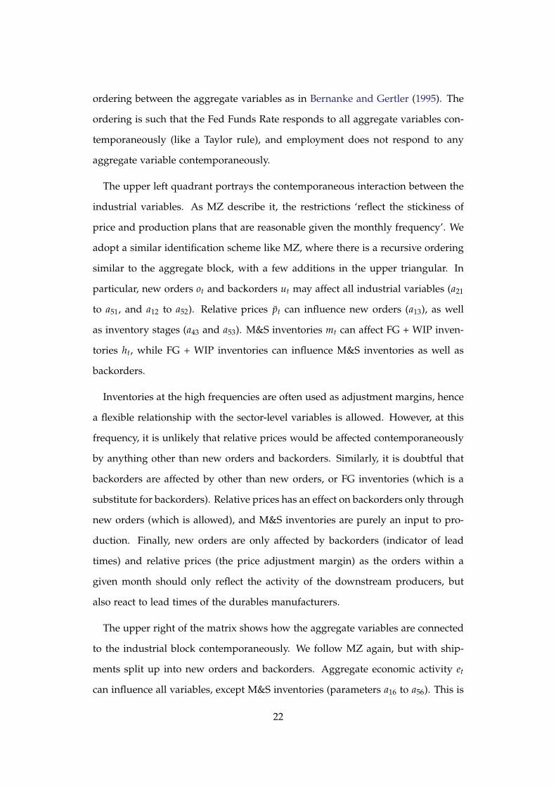
ordering between the aggregate variables as in Bernanke and Gertler (1995). The

ordering is such that the Fed Funds Rate responds to all aggregate variables con-

temporaneously (like a Taylor rule), and employment does not respond to any

aggregate variable contemporaneously.

The upper left quadrant portrays the contemporaneous interaction between the

industrial variables. As MZ describe it, the restrictions ‘reflect the stickiness of

price and production plans that are reasonable given the monthly frequency’. We

adopt a similar identification scheme like MZ, where there is a recursive ordering

similar to the aggregate block, with a few additions in the upper triangular. In

particular, new orders ot and backorders ut may affect all industrial variables (a21

to a51, and a12 to a52). Relative prices p̄t can influence new orders (a13), as well

as inventory stages (a43 and a53). M&S inventories mt can affect FG + WIP inven-

tories ht, while FG + WIP inventories can influence M&S inventories as well as

backorders.

Inventories at the high frequencies are often used as adjustment margins, hence

a flexible relationship with the sector-level variables is allowed. However, at this

frequency, it is unlikely that relative prices would be affected contemporaneously

by anything other than new orders and backorders. Similarly, it is doubtful that

backorders are affected by other than new orders, or FG inventories (which is a

substitute for backorders). Relative prices has an effect on backorders only through

new orders (which is allowed), and M&S inventories are purely an input to pro-

duction. Finally, new orders are only affected by backorders (indicator of lead

times) and relative prices (the price adjustment margin) as the orders within a

given month should only reflect the activity of the downstream producers, but

also react to lead times of the durables manufacturers.

The upper right of the matrix shows how the aggregate variables are connected

to the industrial block contemporaneously. We follow MZ again, but with ship-

ments split up into new orders and backorders. Aggregate economic activity et

can influence all variables, except M&S inventories (parameters a16 to a56). This is

22

the crucial variable that transmits demand into the sector. It is unlikely to affect

M&S inventories as it is an input to production which is likely to be sticky within

one month. The aggregate price level pt can affect the relative price level (a37)

and commodity prices pct can alter the M&S inventories (a48). The aggregate price

level is a component of the relative price level, thus allowing a contemporaneous

relationship is sensible. The commodity price index proxies the acquisition cost of

M&S inventories, hence permitting contemporaneous correlation for the pair. The

zeros in this quadrant is reflective of the simple intuition that the aggregate block

drives the demand for durables (ie. new orders) only through economic activity,

while the variables within the aggregate block can affect each other through the

recursive ordering.

The lag order for this monthly VAR is chosen by AIC (Ivanov and Kilian, 2005).

Searching on a grid of asymmetric lags on the industry-level and aggregate vari-

ables results in two lags each for the HV period, and an asymmetric two and

three lags for industry and aggregate blocks, respectively, in the LV period. Thus,

we estimate the SVARs with the latter’s asymmetric lag structure (2 lags on in-

dustry, 3 on the aggregate block). MZ has more asymmetry in the lags (four on

industry, and seven on the aggregate). The reason that the lags suggested by AIC

is smaller could be due to the large increase of the parameters to be estimated

from adding one variable, into a nine-variable VAR. Using other (harsher) criteria

such as Hannan-Quinn or Schwarz-Bayes results in a much shorter lag structure,

which would be unlikely to capture the true data-generating process given the

monthly frequency. Nevertheless, the main results are robust to a variety of other

lag structures.10

4.3. Counterfactuals Methodology

The counterfactuals method as in Stock and Watson (2003) can disentangle if

industry-level structure (affected by new business practices), or macro effects,

10The results were checked to be robust under symmetric VARs with 2, 3, 4 and 6 lags.

23

produces the fall in volatilities. For this exercise we will measure the decline

in volatility using the forecast root mean squared errors (RMSE).11

To narrow down the mechanisms that drive the results of the counterfactuals, we

examine the impulse responses (defined as % deviation) of the aggregate variables

(Figure 2), as well as industry-level variables (Figures 3 and 4) to a 100 bps Federal

Funds Rate increase.18 The caveat with IRF analysis is that the confidence bands

are typically large, so IRFs cannot be taken as full, conclusive evidence on the

mechanisms.

264

xt

yt

375 =

264

A11(L) A12(L)

0 A22(L)

375 ·

264

xt�1

yt�1

375 + A�1

0 B

264

#t

nt

375 (4)

Better business practices

(micro)

Better policy

(macro)

Good luck

5. Results

Relative RMSECounterfactuals [GLV , LHV ] [GLV , LLV ] [GLV , LLV ]

Micro Macro TotalNew Orders oit 0.72 0.79 0.59Backorders uit 0.83 1.14 0.70

Relative price pit 1.34 0.54 0.78M&S Inventory mit 1.77 1.07 1.21

FG Inventory hit 1.33 2.1 1.21

Table 1: 60-month RMSE counterfactuals of micro vs. macro effectsNotes: The RMSEs are relative to the HV variances and parameters, ie.

⇥QHV

i , SHVi

⇤.

18IRFs to a 1% commodities price increase can be found in the appendices (Figures 11 to 10)

14






mechanisms.

264

xt

yt

375 =

264

A11(L) A12(L)

0 A22(L)

375 ·

264

xt�1

yt�1

375 + A�1

0 B

264

#t

nt

375 (4)


(micro)

Better policy

(macro)

Good luck

5. Results






⇥QHV

i , SHVi

⇤.


14






mechanisms.

264

xt

yt

375 =

264

A11(L) A12(L)

0 A22(L)

375 ·

264

xt�1

yt�1

375 + A�1

0 B

264

#t

nt

375 (4)


(micro)

Better policy

(macro)

Good luck

5. Results






⇥QHV

i , SHVi

⇤.


14






mechanisms.

264

xt

yt

375 =

264

A11(L) A12(L)

0 A22(L)

375 ·

264

xt�1

yt�1

375 + A�1

0 B

264

#t

nt

375 (4)


(micro)

Better policy

(macro)

Good luck

5. Results






⇥QHV

i , SHVi

⇤.


14






mechanisms.

264

xt

yt

375 =

264

A11(L) A12(L)

0 A22(L)

375 ·

264

xt�1

yt�1

375 + A�1

0 B

264

#t

nt

375 (4)


(micro)

Better policy

(macro)

Good luck

5. Results






⇥QHV

i , SHVi

⇤.


14






mechanisms.

264

xt

yt

375 =

264

A11(L) A12(L)

0 A22(L)

375 ·

264

xt�1

yt�1

375 + A�1

0 B

264

#t

nt

375 (4)


(micro)

Better policy

(macro)

Good luck

5. Results






⇥QHV

i , SHVi

⇤.


14






mechanisms.

264

xt

yt

375 =

264

A11(L) A12(L)

0 A22(L)

375 ·

264

xt�1

yt�1

375 + A�1

0 B

264

#t

nt

375 (4)


(micro)

Better policy

(macro)

Good luck

5. Results






⇥QHV

i , SHVi

⇤.


14

Figure 6: Effects of the hypotheses on the SVAR (structural version of Equation 4)

Figure 6 shows schematically how the three hypotheses parse into changes in

the SVAR. We will measure the business practices effect in each period j ∈ {HV, LV}using the upper two quadrants of the lagged coefficients {A11,j(L), A12,j(L)}, and

upper two quadrants of the contemporaneous matrix A0,j). The upper right quad-

rant contains the bullwhip effect – the transmission and amplification of down-

stream demand to upstream orders. The upper left quadrant encompasses the

flexible production and effects of reduced delivery times. We donate all the indus-

try level parameters that capture the business practices effects as Γj.

The macro effects are composed of the aggregate level parameters (A22,j(L) and

the lower right quadrant of A0,j), as well as the shocks. The lower right quadrant

parameters incorporate how monetary policy has changed. For the main results,

we are agnostic of the composition of the macro effects between good luck and

good policy, as we are mainly interested in the amount of volatility reduction

that can be allocated to new business practices as opposed to one of the macro

hypotheses. We will collect all the coefficients associated with the macro effects in

Λj.

We use our estimated SVAR for two different counterfactual exercises. First, we

11Following MZ, the horizon used is 60 months ahead. This is long enough such that the forecasterror variances approach the unconditional volatility of the variable, which is what we are interestedin. The results are robust to longer horizons (90 and 120 months).

24

perform a counterfactual analysis. Our two sets of estimated SVAR coefficients

(one for each period) yield two sets of business practices effects, [ΓHV ,ΛHV ], and

two sets of macro effects (policy and shocks), [ΓLV ,ΛLV ].The LV combination gives

lower volatility compared to the HV for most variables. With particular attention

on new orders, we mix between the business practices and macro factors to see

whether practices, or general macroeconomic developments in monetary policy

and shocks, produce the lower volatility.

The second analysis is a more traditional counterfactual between structure and

shocks. This involves grouping the parameters (Aj, Aj(L)) into Θj, to denote the

industry and macroeconomic structure at period j and the structural shocks are

grouped into Σj = B′jBj. We can then perform the counterfactual exercises of what

happens if, for example, only the shocks changed and the structures did not.

Additionally, we examine more standard forecast error variance decomposition

(FEVD) and impulse response analysis. Specifically, to narrow down the mech-

anisms that drive the results of the counterfactuals, we examine the impulse re-

sponses (defined as log-point deviation) of the sector-level variables (Figure 7), as

well as aggregate variables (Figure 8) to a 100 bps Federal Funds Rate increase.12

5. Results

5.1. Evidence of a role for new business practices

This subsection examines to what extent there is evidence of the new business

practices that we have discussed. We explore the existence of the channels posited

through which better business practices can reduce new orders volatility as well

as other supportive evidence in the behaviour of other variables. This section uses

all the analytical tools we just described.

12IRFs to a 1% commodities price increase can be found in the appendices (Figures 11).

25

Relative RMSECounterfactuals [ΓLV , ΛHV ] [ΓHV , ΛLV ] [ΓLV , ΛLV ]

Practices Macro TotalNew Orders ot 0.72 0.79 0.59Backorders ut 0.83 1.14 0.70

Relative price pt 1.34 0.54 0.78M&S Inventory mt 1.77 1.07 1.21

FG Inventory ht 1.33 2.10 1.21

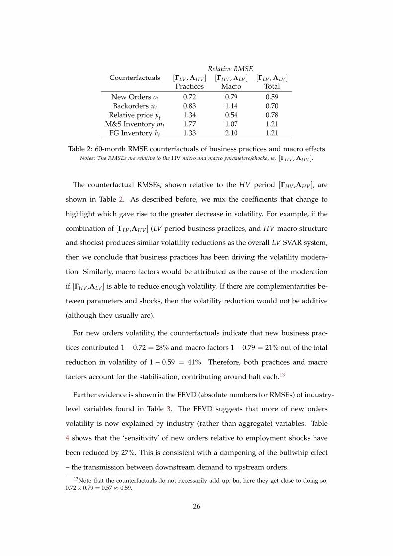
Table 2: 60-month RMSE counterfactuals of business practices and macro effectsNotes: The RMSEs are relative to the HV micro and macro parameters/shocks, ie. [ΓHV , ΛHV ].

The counterfactual RMSEs, shown relative to the HV period [ΓHV ,ΛHV ], are

shown in Table 2. As described before, we mix the coefficients that change to

highlight which gave rise to the greater decrease in volatility. For example, if the

combination of [ΓLV ,ΛHV ] (LV period business practices, and HV macro structure

and shocks) produces similar volatility reductions as the overall LV SVAR system,

then we conclude that business practices has been driving the volatility modera-

tion. Similarly, macro factors would be attributed as the cause of the moderation

if [ΓHV ,ΛLV ] is able to reduce enough volatility. If there are complementarities be-

tween parameters and shocks, then the volatility reduction would not be additive

(although they usually are).

For new orders volatility, the counterfactuals indicate that new business prac-

tices contributed 1− 0.72 = 28% and macro factors 1− 0.79 = 21% out of the total

reduction in volatility of 1 − 0.59 = 41%. Therefore, both practices and macro

factors account for the stabilisation, contributing around half each.13

Further evidence is shown in the FEVD (absolute numbers for RMSEs) of industry-

level variables found in Table 3. The FEVD suggests that more of new orders

volatility is now explained by industry (rather than aggregate) variables. Table

4 shows that the ‘sensitivity’ of new orders relative to employment shocks have

been reduced by 27%. This is consistent with a dampening of the bullwhip effect

– the transmission between downstream demand to upstream orders.

13Note that the counterfactuals do not necessarily add up, but here they get close to doing so:0.72× 0.79 = 0.57 ≈ 0.59.

26

One may worry that the macro factors somehow influence the transmission of

aggregate variables to the sector-level variables (the top right quadrant of pa-

rameters). To address this, we can perform another counterfactual of changing

the upper-left quadrant of parameters only (Table 8 in appendices) – or in other

words, changing specifically the sector-level interactions between the sector vari-

ables. This leaves out a part of the bullwhip effect (the transmission between

aggregate demand to new orders), and emphasises the flexible production and

just-in-time techniques. This alone achieves a 1− 0.82 = 18% reduction in new

orders volatility, demonstrating the strong influence of the within-sector structure

on new orders volatility.

There is also evidence of backordering behaviour change. In the HV period, the

IRFs support the Zarnowitz idea of shipments and production smoothing using

the backorder margin. For a contractionary demand shock (a 100 bps increase

in the Fed Funds Rate), backorders are being run down until new orders start to

recover. This is consistent with large variations in delivery times. However, in

the LV period, backorder levels remain largely stable. In other words, delivery

times become more consistent. More lean production enables faster reaction times

to order disturbances, and customers are more certain they would receive goods

faster and on time. This leads to the dampening of new order volatility.

The evidence of changes in inventory behaviour is, as the earlier analysis sug-

gested, more complicated. The behaviour of M&S inventories and FG + WIP

inventories are very similar. With the negative demand shock, all types of inven-

tory stocks rise in the short term more in the LV period, before falling to suit the

lower level of orders. However, the interpretation of this result is fundamentally

different, as M&S inventories are inputs to the production stage, and FG + WIP

are production outputs.

27

Forecast Variance Decomposition (%)RMSE Own ot ut Other Industry Aggregate

High VolatilityNew Orders ot 1.6 0.4 1.5 4.0 94.1Backorders ut 1.3 0.4 18.0 5.9 75.7

Relative price pt 0.5 6.1 0.1 0.2 0.0 93.6M&S Inventory mt 0.6 3.0 0.2 14.2 5.9 76.7

FG Inventory ht 0.7 12.2 0.2 0.4 10.0 77.1Low Volatility

New Orders ot 0.9 1.2 1.8 11.8 85.3Backorders ut 0.9 0.1 4.6 8.6 86.8

Relative price pt 0.4 34.1 0.2 0.7 0.3 64.7M&S Inventory mt 0.7 6.6 0.1 0.8 20.0 72.4

FG Inventory ht 0.8 2.0 0.1 0.0 8.1 89.8

Table 3: Forecast Error Variance Decomposition

Industry Aggregateot ut pt mt ht et pt pC

t rt

New Orders ot 1.11 0.46 1.12 2.33 0.35 0.73 0.72 0.02 0.12Backorders ut 0.06 0.19 1.50 2.36 0.04 1.04 1.64 0.03 0.15

Relative price pt 1.37 2.16 2.40 1.67 15.81 0.2 2.2 0.01 0.72M&S Inventory mt 1.26 0.09 39.4 1.18 0.09 5.62 1.58 0.11 3.33

FG Inventory ht 0.53 0.23 1.07 2.88 0.41 7.84 1.65 0.11 0.75

Table 4: 60-month horizon relative sensitivity to structural shocksNotes: The sensitivity measures how the volatility of one variable (rows) is driven by a

standardised shock of a particular variable (columns). See Simon (2001) for details on thecalculation. The table reports the ratio of the sensitivity between the LV and HV periods:

a ratio less than one indicates that the variable is less sensitive in the LV period.

For M&S inventories, there could be two channels operating. Firstly, with better

supply chain management, as well as reduced and consistent lead times, lead to

more stable M&S inventory stocks as firms’ suppliers can vary shipments faster as

necessary. The second channel could be that flexible production leads to to man-

ufacturers’ consuming inputs with greater fluctuations, leading to more volatile

inventories.14 Given that M&S inventories are more volatile in the LV period,

this suggests that the latter channel is dominant. The IRFs show that there is an

accumulation of M&S inventories as new orders fall, suggesting that firms are cut-

14A prediction of McMahon (2012) is when inventories become more flexible, they are morevolatile.

28

ting production faster (and symmetrically, are able to increase production quickly

when there is a positive demand shock). Furthermore, despite the increase in

structural shock variance, the counterfactuals indicate that overwhelmingly micro

factors are responsible for the higher volatility (in contrast to FG + WIP invento-

ries). This hints that flexible production techniques are operating in the LV period.

On the other hand, FG + WIP inventory dynamics play a role in stabilising pro-

duction. However, the channel is somewhat different from MZ. The similarity is

that we also find that FG + WIP inventories become more countercyclical with

respect to new orders in the LV period. That is, inventories rise initially with the

fall in new orders, before eventually declining when new orders start recovering.

In contrast to MZ, all inventory type stocks become more volatile. The counter-

factuals suggest that for FG + WIP inventories, this mostly comes from the macro

factors (and from the conventional counterfactuals, aggregate structure) – hence

this supports MZ’s assertion that firms expect less persistent sales shocks, the per-

ceived benefits of maintaining stable production increases. Combine the four facts

that: the RMSEs (which approximates unconditional volatility) of inventories are

much smaller than the RMSE for new orders; that inventories IRF rose by 0.2%

while new orders fell by 0.5% in the LV period, in contrast to a negligible response

of inventories with a 1% fall in new orders in the HV period; it is inventory in-

vestment that enters the production identity; and finally, inventory-sales ratios for

durables hover around two. It is likely that the net effect of FG + WIP inventory

dynamics to be more production smoothing.

As also found in MZ’s IRFs, the HV period impulse responses behave almost

cyclical (especially for new orders), although they decay back to zero after some

periods. IRFs to sector-level variable shocks do not show this behaviour, thus this

feature is driven from the aggregate block. In particular, the economic activity in-

dicator exhibit the same wave as new orders, as well as aggregate and commodity

prices with congruent timing of the troughs and peaks. However, could this be

caused by fluctuating economic activity driving the swings in prices, or is the vari-

29

New Orders Backorders

Relative Price M&S Inventories

FG + WIP Inventories

−0.010

−0.005

0.000

0.005

0.010

−0.010

−0.005

0.000

0.005

−0.002

−0.001

0.000

0.001

0.002

0.003

−0.0075

−0.0050

−0.0025

0.0000

0.0025

−0.004

−0.002

0.000

0.002

0 20 40 60 0 20 40 60

0 20 40 60 0 20 40 60

0 20 40 60

Horizon

Period HV LV

Figure 7: Durables impulse response to a 100 bps Fed Funds Rate increase

30

ability in prices inducing fluctuations in economic activity? The literature suggests

a possible channel for the latter – the indeterminacy of the monetary policy rule in

the HV period (the pre-Volcker era). For example, Lubik and Schorfheide (2004),

Sims and Zha (2006) and others have documented that during the HV period the

Federal Reserve did not increase nominal rates aggressively enough in response

to a rise in inflation. This induces business-cycle fluctuations in output and infla-

tion that would not occur if determinacy was satisfied. The IRFs to a commodity

price shock (Figure 11) is consistent with this story. A 1% increase in commodity

prices induces a large increase in aggregate prices, and also large fluctuations in

economic activity, in the HV period. Meanwhile, in the LV period, a credible and

aggressive Federal Reserve anchored inflation expectations such that the impact

on aggregate prices and economic activity was negligible.

Taken overall, the main conclusion is that there is evidence for lean produc-

tion and micro structural changes lead to more stable orders. Firms are more

inclined to use FG inventories rather than backorders to stabilise production in

the LV period. Greater flexibility in production processes and supply chain man-

agement leads to these dynamics, and in turn, this changes ordering behaviour

such that it stabilises production. The results in Stock and Watson (2003) suggest

that the durables good sector contributed to approximately half the overall out-

put volatility moderation, despite its small relatively size.15 Extending business

practices to include supply chain management, our results suggest that business

practices is responsible for approximately 40-50%. Combining the two, business

practices have contributed to at least 20-25% of the overall Great Moderation. Bet-

ter practices could have contributed more, through other sectors, or in other ways.

Defining business practices as the changes in the sector-level parameters may or

may not pick up the effects of better cash flow management, better hedging and

others.

15See appendices for calculations.

31

5.2. Evidence for macro effects

The previous subsection has highlighted that not only business practices con-

tributed to the Great Moderation, but also the decline in aggregate demand volatil-

ity. We present evidence that supports both the narrative-based literature (that the

Great Moderation emanates from better monetary policy), as well as the VAR-

based literature (that it was good luck).

The counterfactuals and IRFs suggest that the underlying macroeconomic back-

ground that feeds demand shocks into the industry-level variables has changed.

The first point is that there is a large reduction in shocks. The structural variances

of Table 5 indicates that the standard deviation of employment shocks fell by 38%

in the LV period, and commodities price shocks by 25%. Like most VAR-based

studies, this particular result is reconcilable with the good luck hypothesis.

Durables SVARIndustry Block Aggregate BlockShock to Ratio Shock to Ratio

New Orders ot 0.83 Employment et 0.62Backorders ut 0.80 Aggregate price pt 1.01

Relative price pt 1.01 Commodities price pct 0.75

M&S Inventory mt 2.47 Fed Funds Rate rt 0.97FG Inventory ht 0.60

Table 5: Relative size of structural shocks, where Ratio = σ(LV)/σ(HV)

However, it must be remarked that employment is an imperfect indicator of

overall economic activity – greater labour market flexibility may induce greater

employment volatility. The focus of the paper instead is on the components of

sector-level durable goods production, which we know to be a large contributor

of the Great Moderation.

32

Employment Aggregate Price

Commodities Price Fed Funds Rate

−0.002

−0.001

0.000

0.001

−5e−04

0e+00

5e−04

1e−03

−0.0025

0.0000

0.0025

−0.5

0.0

0.5

1.0

1.5

0 20 40 60 0 20 40 60

0 20 40 60 0 20 40 60Horizon

Period HV LV

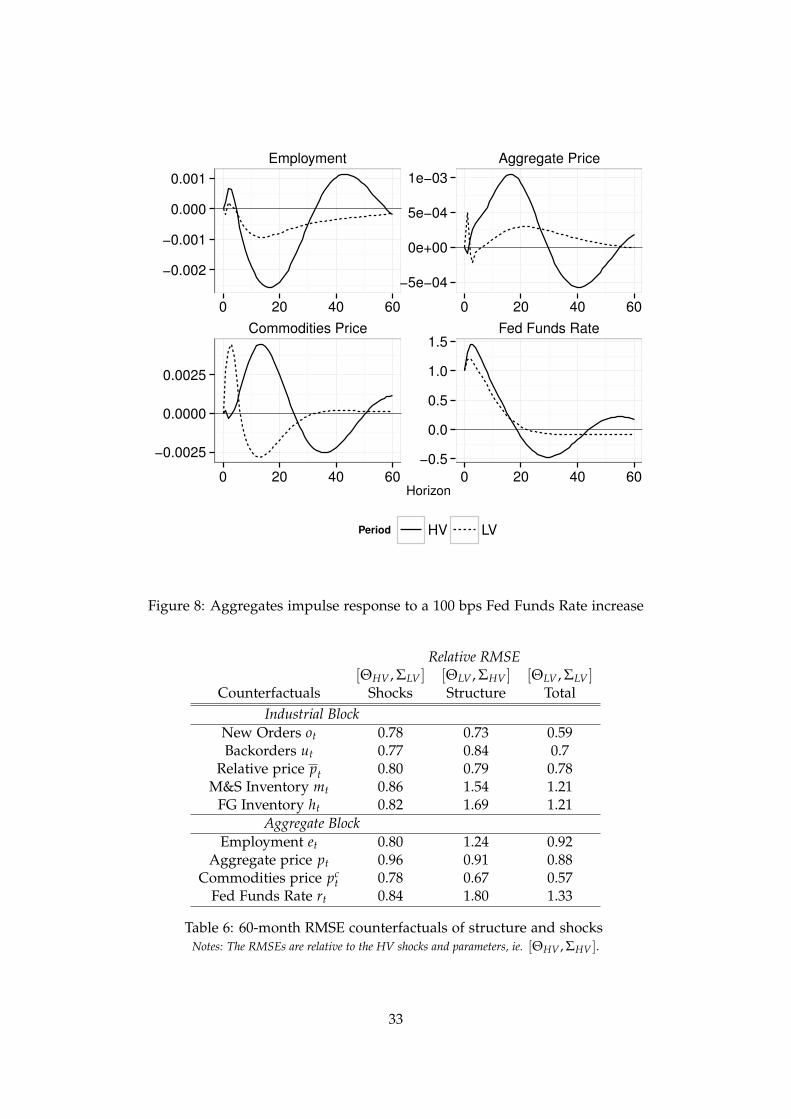
Figure 8: Aggregates impulse response to a 100 bps Fed Funds Rate increase

Relative RMSE[ΘHV , ΣLV ] [ΘLV , ΣHV ] [ΘLV , ΣLV ]

Counterfactuals Shocks Structure TotalIndustrial Block

New Orders ot 0.78 0.73 0.59Backorders ut 0.77 0.84 0.7


FG Inventory ht 0.82 1.69 1.21Aggregate Block

Employment et 0.80 1.24 0.92Aggregate price pt 0.96 0.91 0.88

Commodities price pct 0.78 0.67 0.57

Fed Funds Rate rt 0.84 1.80 1.33

Table 6: 60-month RMSE counterfactuals of structure and shocksNotes: The RMSEs are relative to the HV shocks and parameters, ie. [ΘHV , ΣHV ].

33

On the other hand, unlike VAR-based evidence and similar to narrative-based

evidence, we find significant aggregate structural changes. Firstly, the response of

economic activity to monetary policy shocks in the LV period is much more muted.

Secondly, the response of economic activity to a commodities price shock (Figure

11) reveals how better monetary policy affects the economy differently. Commod-

ity price shocks no longer cause economic activity fluctuations (or aggregate price

level). This offers evidence that the macro structure has changed to stabilise ex-

ogenous shocks better. Noting the counterfactual (Table 6) that macroeconomic

structure increases Federal Funds Rate volatility, this suggests that the Federal Re-

serve became more responsive to movements in output and inflation. This is con-

sistent with past literature – for example, Clarida, Galí, and Gertler (2000), Boivin

and Giannoni (2002), Lubik and Schorfheide (2004) – that suggests the Federal Re-

serve’s reaction function parameter to inflation have increased, and also Watson

(1999) that the Federal Funds Rate became more persistent. Greater response and

persistence induces more variability in the Federal Funds Rate. Thus, the isolation

of the macroeconomic system from exogenous shocks appears to resulted from

the Federal Reserve’s credibility in fighting inflation.

This is also supported by the counterfactuals of commodity price forecast er-

rors. Shocks contribute to some reduction in volatility, but it is mostly from the

sensitivity of the system (see Table 4). This explains why LV period impulse re-

sponses of all variables are much more muted, as well as returning to zero faster.

Credible monetary policy anchored inflation expectations and price shocks do not

become persistent. This is consistent with the results in McCarthy and Zakrajšek

(2003) and Bernanke and Gertler (1995), where they found that aggregate output

and prices responded less to oil price shocks post-1985.

Therefore, the results are consistent with the hypothesis that an aggressive Fed-

eral Reserve stance stabilised the macroeconomic system, deriving from reduc-

ing the impact of exogenous price shocks on real variables, rather than directly

smoothing output.

34

6. Conclusion

In this paper, we revisit the important question of what gave rise to the Great

Moderation. In particular, our main contribution is to extend the definition of

new business practices to include aspects of supply chain management that fit

much more closely with actual changes in practice than simply better inventory

management practices.

Our empirical work analysis supports a much greater role for new business

practices in attenuating sales volatility in the durable manufacturing sector than

most of the earlier literature. Our evidence is consistent with a reduction of the

bullwhip effect and the effects of flexible production.

Most of the Great Moderation is still caused by the main macro factors – good

luck and monetary policy. We present evidence that both play a role. Nevertheless,

our results bring a case for optimism – around a quarter of the volatility reduction

is due to better business practices (20-25%). Unlike the good luck result from

most VAR-based studies, we can expect that this volatility will not easily return as

the new technologies have changed supply chain management, and parts of our

macroeconomic structures, forever.

35

References

Ahmed, S., A. Levin, and B. A. Wilson (2004): “Recent US Macroeconomic Sta-

bility: Good Policies, Good Practices, or Good Luck?,” Review of Economics and

Statistics, 86(3), 824–832.

Alessandria, G., J. Kaboski, and V. Midrigan (2013): “Trade wedges, inven-

tories, and international business cycles,” Journal of Monetary Economics, 60(1),

1–20.

Barth, M. J., and V. A. Ramey (2002): “The cost channel of monetary transmis-

sion,” in NBER Macroeconomics Annual 2001, ed. by B. S. Bernanke, and K. Rogoff,

pp. 199–256. MIT Press, MIT Press.

Bernanke, B. S., and M. Gertler (1995): “Inside the Black Box: The Credit Chan-

nel of Monetary Policy Transmission,” Journal of Economic Perspectives, 9, 24–48.

Blanchard, O. J., and J. Simon (2001): “The Long and Large Decline in US Output

Volatility,” Brookings Papers on Economic Activity, 2001(1), 135–174.

Boivin, J., and M. P. Giannoni (2002): “Has Monetary Policy Become Less Pow-

erful?,” Federal Reserve Bank of New York Staff Report, (144).

(2006): “Has monetary policy become more effective?,” Review of Economics

and Statistics, 88(3), 445–462.

Clarida, R., J. Galí, and M. Gertler (2000): “Monetary Policy Rules and Macroe-

conomic Stability: Evidence and Some Theory,” Quarterly Journal of Economics,

115(1), 147–180.

Cogley, T., and T. J. Sargent (2001): “Evolving Post-World War II US Inflation Dy-

namics,” in NBER Macroeconomics Annual, ed. by B. S. Bernanke, and K. Rogoff,

pp. 331–388. MIT Press.

Davis, S. J., and J. Haltiwanger (2001): “Sectoral job creation and destruction

responses to oil price changes,” Journal of Monetary Economics, 48(3), 465–512.

36

Davis, S. J., and J. A. Kahn (2008): “Interpreting the great moderation: Changes

in the volatility of economic activity at the macro and micro levels,” Journal of

Economic Perspectives, 22, 155–180.

Forrester, J. (1961): Industrial dynamics. Pegasus Communications, Waltham, MA.

Gourieroux, C., and A. Monfort (1997): Time Series and Dynamic Models, Themes

in Modern Econometrics. Cambridge University Press.

Herrera, A. M., and E. Pesavento (2005): “The Decline in U.S. Output Volatility,”

Journal of Business & Economic Statistics, 23(4), 462–472.

Ivanov, V., and L. Kilian (2005): “A Practitioner’s Guide to Lag Order Selection

for VAR Impulse Response Analysis,” Studies in Nonlinear Dynamics & Economet-

rics, 9(1).

Kahn, J. A., M. McConnell, and G. Perez-Quiros (2002): “On the Causes of

the Increased Stability of the US Economy,” Federal Reserve Bank of New York,

Economic Policy Review, 8(1), 183–202.

Khan, A., and J. Thomas (2007): “Inventories and the business cycle: An equilib-

rium analysis of (S, s) policies,” American Economic Review, pp. 1165–1188.

Kim, C.-J., C. R. Nelson, and J. Piger (2004): “The Less-Volatile US Economy: a

Bayesian Investigation of Timing, Breadth, and Potential Explanations,” Journal

of Business & Economic Statistics, 22(1), 80–93.

Lee, H. L., V. Padmanabhan, and S. Whang (2004): “Information Distortion in

a Supply Chain: The Bullwhip Effect,” Management Science, 50(12 Supplement),

1875–1886.

Lubik, T. A., and F. Schorfheide (2004): “Testing for indeterminacy: An applica-

tion to US monetary policy,” American Economic Review, pp. 190–217.

37

McCarthy, J., and E. Zakrajšek (2003): “Inventory Dynamics and Business Cy-

cles: What Has Changed?,” Board of Governors of the Federal Reserve System Fi-

nance and Economics Discussion Series, 26.

McCarthy, J., and E. Zakrajšek (2007): “Inventory Dynamics and Business Cy-

cles: What Has Changed?,” Journal of Money, Credit and Banking, 39(2), 591–613.

McConnell, M., and G. Perez-Quiros (2000): “Output Fluctuations in the United

States: What Has Changed Since the Early 1980’S?,” American Economic Review,

90(5), 1464–1476.

McMahon, M. (2012): “Inventories in Motion: A New Approach To Inventories

Over The Business Cycle,” .

Orphanides, A. (2004): “Monetary Policy Rules, Macroeconomic Stability, and

Inflation: a View From the Trenches,” Journal of Money, Credit and Banking, 36(2),

151–175.

Simon, J. (2001): “The Decline in Australian Output Volatility,” Reserve Bank of

Australia Research Discussion Paper, 1.

Sims, C. A., and T. Zha (2006): “Were there regime switches in US monetary

policy?,” American Economic Review, pp. 54–81.

Song, J.-S., H. Zhang, Y. Hou, and M. Wang (2010): “The Effect of Lead Time and

Demand Uncertainties in (r, q) Inventory Systems,” Operations Research, 58(1),

68–80.

Song, J.-S., and P. H. Zipkin (1996): “The Joint Effect of Leadtime Variance and

Lot Size in a Parallel Processing Environment,” Management Science, 42(9), 1352–

1363.

Stock, J. H., and M. W. Watson (2003): “Has the Business Cycle Changed and

Why?,” in NBER Macroeconomics Annual 2002, Volume 17, ed. by M. Gertler, and

K. Rogoff, pp. 159–230. MIT press.

38

Taylor, J. B. (2013): “The Effectiveness of Central Bank Independence Versus Pol-

icy Rules ,” in American Economic Association Annual Meeting, San Diego, CA.

Watson, M. W. (1986): “Univariate Detrending Methods with Stochastic Trends,”

Journal of Monetary Economics, 18(1), 49–75.

(1999): “Explaining the Increased Variability in Long-Term Interest Rates,”

FRB Richmond Economic Quarterly, 85(4), 71–96.

Zarnowitz, V. (1962): “Unfilled Orders, Price Changes, and Business Fluctua-

tions,” Review of Economics and Statistics, 44(4), 367–394.

39

A. Appendix

1

2

3

4

5

1970 1975 1980 1985 1990 1995Time

32M 33M 34M

Backorders−Sales Ratios for Disaggregated Durables

3

6

9

1970 1975 1980 1985 1990 1995Time

35M 36M 37M 38M

Backorders−Sales Ratios for Disaggregated Durables

Figure 9: Disaggregated Backorders to Shipments RatioSIC codes: 32M – Stone, Clay and Glass, 33M – Primary metals, 34M – Fabricated metals,

35M – Industrial machinery and equipment, 36M – Electronic and other electricalequipment, 37M – Transportation equipment, 38M – Instruments and related products.

40

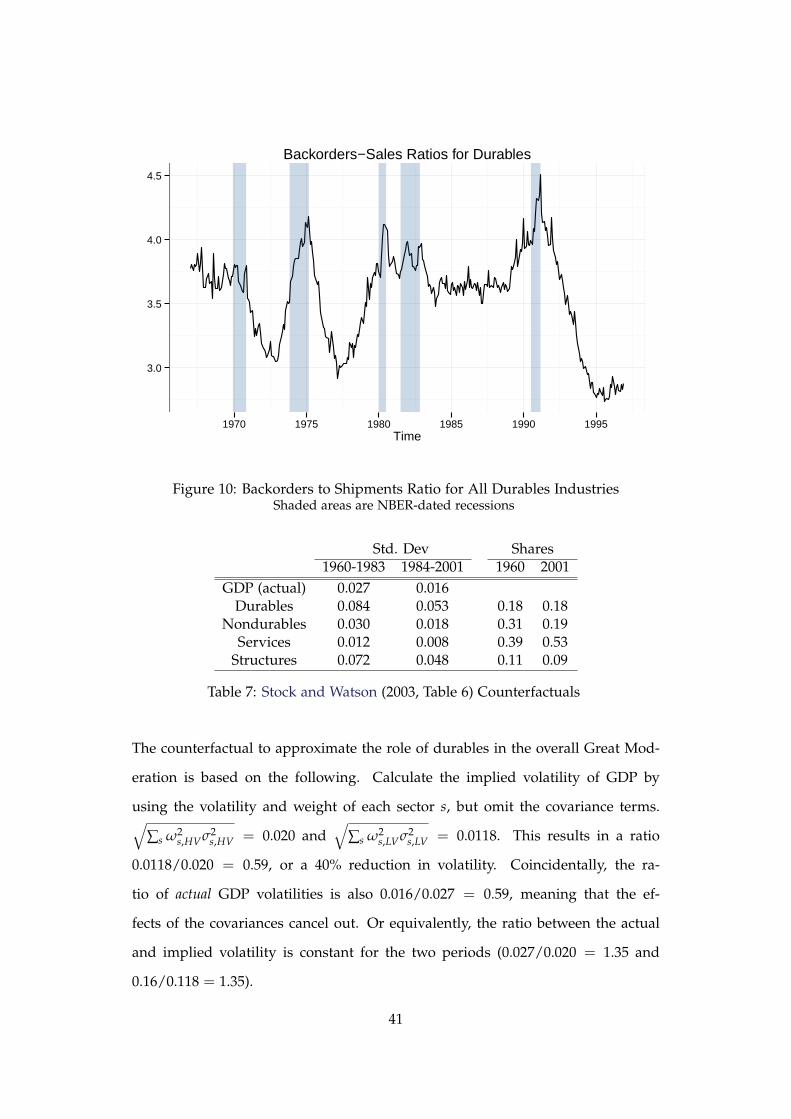
3.0

3.5

4.0

4.5

1970 1975 1980 1985 1990 1995Time

Backorders−Sales Ratios for Durables

Figure 10: Backorders to Shipments Ratio for All Durables IndustriesShaded areas are NBER-dated recessions

Std. Dev Shares1960-1983 1984-2001 1960 2001

GDP (actual) 0.027 0.016Durables 0.084 0.053 0.18 0.18

Nondurables 0.030 0.018 0.31 0.19Services 0.012 0.008 0.39 0.53

Structures 0.072 0.048 0.11 0.09

Table 7: Stock and Watson (2003, Table 6) Counterfactuals

The counterfactual to approximate the role of durables in the overall Great Mod-

eration is based on the following. Calculate the implied volatility of GDP by

using the volatility and weight of each sector s, but omit the covariance terms.√

∑s ω2s,HVσ2

s,HV = 0.020 and√

∑s ω2s,LVσ2

s,LV = 0.0118. This results in a ratio

0.0118/0.020 = 0.59, or a 40% reduction in volatility. Coincidentally, the ra-

tio of actual GDP volatilities is also 0.016/0.027 = 0.59, meaning that the ef-

fects of the covariances cancel out. Or equivalently, the ratio between the actual

and implied volatility is constant for the two periods (0.027/0.020 = 1.35 and

0.16/0.118 = 1.35).

41

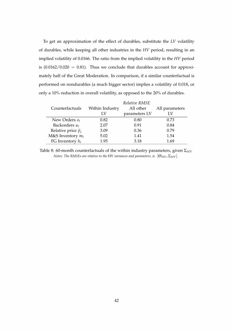
To get an approximation of the effect of durables, substitute the LV volatility

of durables, while keeping all other industries in the HV period, resulting in an

implied volatility of 0.0166. The ratio from the implied volatility in the HV period

is (0.0162/0.020 = 0.81). Thus we conclude that durables account for approxi-

mately half of the Great Moderation. In comparison, if a similar counterfactual is

performed on nondurables (a much bigger sector) implies a volatility of 0.018, or

only a 10% reduction in overall volatility, as opposed to the 20% of durables.

Relative RMSECounterfactuals Within Industry All other All parameters

LV parameters LV LVNew Orders ot 0.82 0.80 0.73Backorders ut 2.07 0.91 0.84



Table 8: 60-month counterfactuals of the within industry parameters, given ΣHVNotes: The RMSEs are relative to the HV variances and parameters, ie. [ΘHV , ΣHV ].

42

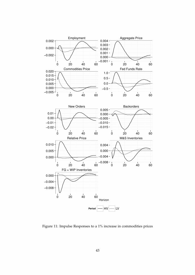
Employment Aggregate Price

Commodities Price Fed Funds Rate

−0.002

0.000

0.002

−0.001

0.000

0.001

0.002

0.003

0.004

−0.005

0.000

0.005

0.010

0.015

0.020

−0.5

0.0

0.5

1.0

0 20 40 60 0 20 40 60

0 20 40 60 0 20 40 60




−0.02

−0.01

0.00

0.01

−0.015

−0.010

−0.005

0.000

0.005

0.000

0.005

0.010

−0.008

−0.004

0.000

0.004

−0.008

−0.004

0.000

0 20 40 60 0 20 40 60

0 20 40 60 0 20 40 60

0 20 40 60

Horizon

Period HV LV

Figure 11: Impulse Responses to a 1% increase in commodities prices

43

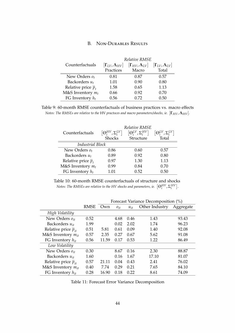
B. Non-Durables Results

Relative RMSECounterfactuals [ΓLV , ΛHV ] [ΓHV , ΛLV ] [ΓLV , ΛLV ]

Practices Macro TotalNew Orders ot 0.81 0.87 0.57Backorders ut 1.01 0.90 0.80



Table 9: 60-month RMSE counterfactuals of business practices vs. macro effectsNotes: The RMSEs are relative to the HV practoces and macro parameters/shocks, ie. [ΓHV , ΛHV ].

Relative RMSECounterfactuals

[ΘHV

i , ΣLVi] [

ΘLVi , ΣHV

i] [

ΘLVi , ΣLV

i]

Shocks Structure TotalIndustrial Block

New Orders ot 0.86 0.60 0.57Backorders ut 0.89 0.92 0.80



Table 10: 60-month RMSE counterfactuals of structure and shocksNotes: The RMSEs are relative to the HV shocks and parameters, ie.

[ΘHV

i , ΣHVi].

Forecast Variance Decomposition (%)RMSE Own oit uit Other Industry Aggregate

High VolatilityNew Orders oit 0.52 4.68 0.46 1.43 93.43Backorders uit 1.99 0.02 2.02 1.74 96.23

Relative price pit 0.51 5.81 0.61 0.09 1.40 92.08M&S Inventory mit 0.57 2.35 0.27 0.67 5.62 91.08

FG Inventory hit 0.56 11.59 0.17 0.53 1.22 86.49Low Volatility

New Orders oit 0.30 8.67 0.16 2.30 88.87Backorders uit 1.60 0.16 1.67 17.10 81.07

Relative price pit 0.57 21.11 0.04 0.43 2.41 76.02M&S Inventory mit 0.40 7.74 0.29 0.21 7.65 84.10

FG Inventory hit 0.28 16.90 0.18 0.22 8.61 74.09

Table 11: Forecast Error Variance Decomposition

44




−0.004

−0.002

0.000

0.002

−0.010

−0.005

0.000

0.005

0.010

−0.003

0.000

0.003

0.006

−0.0075

−0.0050

−0.0025

0.0000

0.0025

−0.009

−0.006

−0.003

0.000

0 20 40 60 0 20 40 60

0 20 40 60 0 20 40 60

0 20 40 60

Horizon

Period HV LV

Figure 12: Non-durables Impulse Responses to a 100 bps Fed Funds Rate Increase

45

beyond inventory management: the bullwhip effect and the

Documents