beyond equilibrium: predicting human behavior in …kevinlb/talks/2012-oplog-talk.pdf · beyond...

Introduction Models Model Comparisons Bayesian Analysis

Beyond Equilibrium:Predicting Human Behavior in Normal-Form Games

Kevin Leyton-Brown, University of British Columbia

Based on joint work with James R. Wright

OpLog Seminar, September 10, 2012

September 10, 2012: OpLog Kevin Leyton-Brown


Overview

1 Introduction

2 Models of Human Behavior in Simultaneous-Move Games

3 Comparing our Models in Terms of Predictive Performance

4 Digging Deeper: Bayesian Analysis of Model Parameters



Context

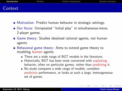
Motivation: Predict human behavior in strategic settings.

Our focus: Unrepeated “initial play” in simultaneous-move,2-player games.

Game theory: Studies idealized rational agents, not humanagents.

Behavioral game theory: Aims to extend game theory tomodeling human agents.

There are a wide range of BGT models in the literature.Historically, BGT has been most concerned with explainingbehavior, often on particular games, rather than predicting it.No study compares a wide range of models, considerspredictive performance, or looks at such a large, heterogeneousset of games.



Contribution

Our contributions:

Compared predictive performance of the most prominentsolution concepts for our setting:

Nash equilibrium, plusFour models from behavioral game theory

. . . using nine experimental datasets from the literature

Bayesian sensitivity analysis:

Yields new insight into existing model (Poisson-CH)Argues for a novel simplification of an existing model(Quantal level-k)



Overview

1 Introduction






Example: Traveler’s Dilemma

2 3 4 96 97 98 99 100. . .

100

100

96 + 2 = 98

96− 2 = 94 100

100

99− 2 = 97

99 + 2 = 101

98 + 2 = 100

98− 2 = 96

2

2

Two players pick a number (2-100) simultaneously.

If they pick the same number, that is their payoff.

If they pick different numbers:

Lower player gets lower number, plus bonus of 2.Higher player gets lower number, minus penalty of 2.




2 3 4 96 97 98 99 100. . .

100

100

96 + 2 = 98

96− 2 = 94

100

100

99− 2 = 97

99 + 2 = 101

98 + 2 = 100

98− 2 = 96

2

2








2 3 4 96 97 98 99 100. . .

100

100

96 + 2 = 98

96− 2 = 94 100

100

99− 2 = 97

99 + 2 = 101

98 + 2 = 100

98− 2 = 96

2

2








2 3 4 96 97 98 99 100. . .

100

100

96 + 2 = 98

96− 2 = 94

100

100

99− 2 = 97

99 + 2 = 101

98 + 2 = 100

98− 2 = 96

2

2





Traveler’s Dilemma has a unique Nash equilibrium.




2 3 4 96 97 98 99 100. . .

100

100

96 + 2 = 98

96− 2 = 94 100

100

99− 2 = 97

99 + 2 = 101

98 + 2 = 100

98− 2 = 96

2

2





Traveler’s Dilemma has a unique Nash equilibrium.



Nash equilibrium and human subjects

Nash equilibrium often makes counterintuitive predictions.

In Traveler’s Dilemma: The vast majority of human playerschoose 97–100. The Nash equilibrium is 2.

Modifications to a game that don’t change Nash equilibriumpredictions at all can cause large changes in how humansubjects play the game [Goeree & Holt 2001].

In Traveler’s Dilemma: When the penalty is large, people playmuch closer to Nash equilibrium.But the size of the penalty does not affect equilibrium.

Clearly Nash equilibrium is not the whole story.

Behavioral game theory proposes a number of models tobetter explain human behavior.



BGT model: Quantal response equilibrium (QRE)

Cost-proportional errors: Agents are less likely to make high-costmistakes than low-cost mistakes.

QRE model [McKelvey & Palfrey 1995] parameter: (λ)

Agents quantally best respond to each other.

QBRi(s−i, λ)(ai) =eλui(ai,s−i)∑

a′i∈Aieλui(a

′i,s−i)

Precision parameter λ ∈ [0,∞) indicates how sensitive agentsare to utility differences.

λ = 0 means agents choose actions uniformly at random.As λ→∞, QBR approaches best response.



Nice story—but is QRE a good model?

Let’s say we pay a bunch of people to play games against eachother, and gather some data. Now we’d like to know how good ajob our QRE model does. How would we do that?

Two issues:

have to set the model’s parameter (λ) to use it at all;

must ensure that we do this in a way that generalizes to newplay by the same people.



Scoring a model’s performance

We randomly partition our data into different sets:D = Dtrain ∪ DtestWe choose parameter value(s) that maximize the likelihood ofthe training data:

#»

θ ∗ = argmax#»θ

Pr(Dtrain |M,#»

θ ).

a tricky non-convex optimization problem

We score the performance of a model by the likelihood of thetest data:

Pr(Dtest |M,#»

θ ∗).

To reduce variance, we repeat this process multiple times withdifferent random partitions and average the results



BGT models: Iterative strategic reasoning

Level-0 agents choose actions non-strategically.

In this work (and most others), uniformly at random

Level-1 agents reason about level-0 agents.

Level-2 agents reason about level-1 agents.

There’s a probability distribution over levels.

Higher-level agents are “smarter”; scarcer

Predicting the distribution of play: weighted sum of thedistributions for each level.



BGT model: Lk

Lk model [Costa-Gomes et al. 2001] parameters: (α1, α2, ε1, ε2)

Each agent has one of 3 levels: level-0, level-1, or level-2.

Distribution of level [2, 1, 0] agents is [α2, α1, (1− α1 − α2)]

Each level-k agent makes a “mistake” with prob εk, or bestresponds to level-(k − 1) opponent with prob 1− εk.

Level-k agents believe all opponents are level-(k − 1).Level-k agents aren’t aware that level-(k − 1) agents will make“mistakes”.

IBRi,0 = Ai,

IBRi,k = BRi(IBR−i,k−1),

πLki,0 (ai) = |Ai|−1,

πLki,k (ai) =

{(1− εk)/|IBRi,k| if ai ∈ IBRi,k,εk/(|Ai| − |IBRi,k|) otherwise.



BGT model: Cognitive hierarchy

Cognitive hierarchy model [Camerer et al. 2004] parameter: (τ)

An agent of level m best responds to the truncated, truedistribution of levels from 0 to m− 1.

Poisson-CH: Levels are assumed to have a Poisson distributionwith mean τ .

πPCHi,0 (ai) = |Ai|−1,

πPCHi,m (ai) =

∣∣∣BRi (πPCHi,0:m−1

)∣∣∣−1 if ai ∈ BRi(πPCHi,0:m−1

),

0 otherwise.

πPCHi,0:m−1 =

∑m−1`=0 πPCHi,` Pr(Poisson(τ) = `)∑m−1

`=0 Pr(Poisson(τ) = `)



BGT model: QLk

QLk model [Stahl & Wilson 1994] parameters: (α1, α2, λ1, λ2, λ1(2))

Distribution of level [2, 1, 0] agents is [α2, α1, (1− α1 − α2)]

Each agent quantally responds to next-lower level.

Each QLk agent level has its own precision (λk), and its ownbeliefs about lower-level agents’ precisions (λ`(k)).

πQLki,0 (ai) = |Ai|−1,

πQLki,1 = QBRi(πQLk−i,0 , λ1),

πQLkj,1(2) = QBRj(πQLk−j,0 , λ1(2)),

πQLki,2 = QBRi(πQLk−i,1(2), λ2).



Overview

1 Introduction






Model comparisons: Nash equilibrium vs. BGT

100

1010

1020

1030

1040

1050

1060

COMBO9 SW94 SW95 CGCB98 GH01 HSW01 CVH03 HS07 SH08 RPC09

Like

lihoo

d im

prov

emen

t ove

r uni

form

dis

tribu

tion

NEEBest BGT

Worst BGT

Average NEE virtually always worse than every BGT model(only exception: SW95).

All NEE significantly worse than best BGT model in mostdatasets.



Model comparisons: Lk and CH vs. QRE

100

1010

1020

1030

1040

1050

1060


Like

lihoo

d im

prov

emen

t ove

r uni

form

dis

tribu

tion

LkPoisson-CH

Lk and Poisson-CH performance was strikingly similar.

No consistent ordering between Lk/Poisson-CH and QRE.Iterative strategic reasoning and quantal response appear tocapture distinct phenomena.



Model comparisons: Lk and CH vs. QRE

100

1010

1020

1030

1040

1050

1060


Like

lihoo

d im

prov

emen

t ove

r uni

form

dis

tribu

tion

LkPoisson-CH

QRE

Lk and Poisson-CH performance was strikingly similar.No consistent ordering between Lk/Poisson-CH and QRE.

Iterative strategic reasoning and quantal response appear tocapture distinct phenomena.



Model comparisons: QLk

100

1010

1020

1030

1040

1050

1060


Like

lihoo

d im

prov

emen

t ove

r uni

form

dis

tribu

tion

LkPoisson-CH

QRE

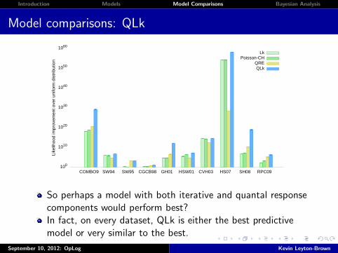
So perhaps a model with both iterative and quantal responsecomponents would perform best?

In fact, on every dataset, QLk is either the best predictivemodel or very similar to the best.



Model comparisons: QLk

100

1010

1020

1030

1040

1050

1060


Like

lihoo

d im

prov

emen

t ove

r uni

form

dis

tribu

tion

LkPoisson-CH

QREQLk

So perhaps a model with both iterative and quantal responsecomponents would perform best?In fact, on every dataset, QLk is either the best predictivemodel or very similar to the best.



Overview

1 Introduction






Taking Stock of What We Have Done

Take-home message so far

QLk is the best of the models for prediction.

Question

How strongly does the data argue for particular parameter values?



Posterior distributions

A posterior distribution gives the probability of each possiblecombination of parameter values, given the data, e.g.:

Pr(α1 = 0.1, α2 = 0.3, λ = 0.1 | D)

Maximum likelihood only tells us the most likely parametersetting, given the data.

The posterior distribution over parameter settings describesthe relative probability of all possible parameter settings.

Individual parameters can be analyzed by inspecting themarginal posterior distribution.

Pr(α1 = 0.1 | D) =∫∫

Pr(α1 = 0.1, α2 = α′2, λ = λ′ | D)dα′2dλ′

Flat distributions indicate less important parameter values.Sharp distributions indicate a high degree of certainty.



Warm-up: Poisson-CH

Regarding the single parameter (τ) for the Poisson-CH model:

“Indeed, values of τ between 1 and 2 explain empiricalresults for nearly 100 games, suggesting that a τ value of1.5 could give reliable predictions for many other gamesas well.” [Camerer et al. 2004]



Warm-up: Poisson-CH’s Posterior Distribution

0

0.2

0.4

0.6

0.8

1

0.48 0.49 0.5 0.51 0.52 0.53 0.54 0.55 0.56 0.57 0.58 0.59 0.6 0.61 0.62

Cum

ulat

ive

prob

abilit

y

τ

Our analysis gives 99% posterior probability that the best value ofτ is 0.59 or less.



Refresher: QLk’s Parameters

QLk has 5 different parameters:

α1: Proportion of level-1 agents.

α2: Proportion of level-2 agents.

λ1: Precision of level-1 agents.

λ2: Precision of level-2 agents.

λ1(2): Level-2 agents’ belief about level-1 agents’ precision.

πQLki,0 (ai) = |Ai|−1,

πQLki,1 = QBRi(πQLk−i,0 , λ1),

πQLkj,1(2) = QBRj(πQLk−j,0 , λ1(2)),

πQLki,2 = QBRi(πQLk−i,1(2), λ2).



Posterior distributions: QLk

0

0.2

0.4

0.6

0.8

1

0 0.1 0.2 0.3 0.4 0.5

Cum

ulat

ive

prob

abilit

y

Level proportions

α1α2

0

0.2

0.4

0.6

0.8

1

0 1 2 3 4 5 6

Cum

ulat

ive

prob

abilit

y

Precisions

λ1λ2λ1(2)

Some surprises:

1 α1, α2: Best fits predict more level-2 agents than level-1.

2 λ1, λ2: Level-2 agents have lower precision than level-1 agents.

3 λ1, λ1(2): Level-2 agents’ beliefs are very wrong.



Maybe QLk isn’t quite the right model

We constructed a family of models by systematically varying QLk:1 Top level:

1, 2, 3, 4, 5, 6, 7, Poisson

2 Precisions: Homogeneous or inhomogeneous.

3 Precision beliefs: Accurate or general.

4 Population beliefs: Lk or CH.

We evaluated all variations leading to ≤ 8 parameters.



Model variations: Efficient frontier

1026

1027

1028

1029

1030

1031

1 2 3 4 5 6 7 8 9 10 11

Like

lihoo

d im

prov

emen

t ove

r u.a

.r.

Number of parameters

Model performance

ah-QLkp

gi-QLk2

ai-QLk2

gh-QLk2

ah-QLk2

gi-QCH2

ai-QCH2

gh-QCH2

ah-QCH2

gi-QLk3

ai-QLk3

ah-QLk3

gi-QCH3

ai-QCH3

ah-QLk4ah-QLk5 ah-QLk6 ah-QLk7

ah-QCH6 ah-QCH7ai-QLk4ai-QCH4

gh-QCH3gh-QLk3

ah-QCHp

ah-QCH3

ah-QCH4

ah-QCH5

Efficient frontier: best performance for # of parameters.

QLk (gi-QLk2) is not on the efficient frontier.

Best models all have accurate precision beliefs, homogeneousprecision, cognitive hierarchy population beliefs.



Model variations: Efficient frontier

1026

1027

1028

1029

1030

1031

1 2 3 4 5 6 7 8 9 10 11

Like

lihoo

d im

prov

emen

t ove

r u.a

.r.


Model performanceEfficient frontier

ah-QLkp

gi-QLk2

ai-QLk2

gh-QLk2

ah-QLk2

gi-QCH2

ai-QCH2

gh-QCH2

ah-QCH2

gi-QLk3

ai-QLk3

ah-QLk3

gi-QCH3

ai-QCH3

ah-QLk4ah-QLk5 ah-QLk6 ah-QLk7

ah-QCH6 ah-QCH7ai-QLk4ai-QCH4

gh-QCH3gh-QLk3

ah-QCHp

ah-QCH3

ah-QCH4

ah-QCH5

Efficient frontier: best performance for # of parameters.

QLk (gi-QLk2) is not on the efficient frontier.

Best models all have accurate precision beliefs, homogeneousprecision, cognitive hierarchy population beliefs.



Thinking back to QLk

0

0.2

0.4

0.6

0.8

1

0 0.1 0.2 0.3 0.4 0.5

Cum

ulat

ive

prob

abilit

y

Level proportions

α1α2

0

0.2

0.4

0.6

0.8

1

0 1 2 3 4 5 6

Cum

ulat

ive

prob

abilit

y

Precisions

λ1λ2λ1(2)

Recall...

α1, α2: Best fits predict more level-2 agents than level-1.

λ1, λ2: Level-2 agents have lower precision than level-1 agents.

λ1, λ1(2): Level-2 agents’ beliefs are very wrong.



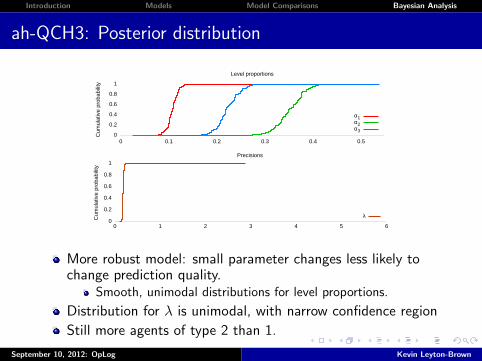
ah-QCH3: Posterior distribution

0

0.2

0.4

0.6

0.8

1

0 0.1 0.2 0.3 0.4 0.5

Cum

ulat

ive

prob

abilit

y

Level proportions

α1α2α3

0

0.2

0.4

0.6

0.8

1

0 1 2 3 4 5 6

Cum

ulat

ive

prob

abilit

y

Precisions

λ

More robust model: small parameter changes less likely tochange prediction quality.

Smooth, unimodal distributions for level proportions.

Distribution for λ is unimodal, with narrow confidence region

Still more agents of type 2 than 1.



Marginal distributions comparison

0 0.2 0.4 0.6 0.8

1

0 0.1 0.2 0.3 0.4 0.5

Cum

ulat

ive

prob

abilit

y

Proportion of L0ah-QCHpah-QCH3ah-QCH4ah-QCH5

0 0.2 0.4 0.6 0.8

1

0 0.1 0.2 0.3 0.4 0.5

Proportion of L1

0 0.2 0.4 0.6 0.8

1

0 0.1 0.2 0.3 0.4 0.5

Proportion of L2

0 0.2 0.4 0.6 0.8

1

0 0.1 0.2 0.3 0.4 0.5

Proportion of L3

0 0.2 0.4 0.6 0.8

1

0 0.1 0.2 0.3 0.4 0.5

Proportion of L4

0 0.2 0.4 0.6 0.8

1

0 0.1 0.2 0.3 0.4 0.5

Proportion of L5

Poisson QCH matches tabular L0 proportions very closely.To do so, forced to match most other proportions poorly.

If L0 were treated specially, could Poisson match others?



Marginal distributions comparison

0 0.2 0.4 0.6 0.8

1

0 0.1 0.2 0.3 0.4 0.5

Cum

ulat

ive

prob

abilit

y

Proportion of L0ah-QCHpah-QCH3ah-QCH4ah-QCH5

0 0.2 0.4 0.6 0.8

1

0 0.1 0.2 0.3 0.4 0.5

Proportion of L1

0 0.2 0.4 0.6 0.8

1

0 0.1 0.2 0.3 0.4 0.5

Proportion of L2

0 0.2 0.4 0.6 0.8

1

0 0.1 0.2 0.3 0.4 0.5

Proportion of L3

0 0.2 0.4 0.6 0.8

1

0 0.1 0.2 0.3 0.4 0.5

Proportion of L4

0 0.2 0.4 0.6 0.8

1

0 0.1 0.2 0.3 0.4 0.5

Proportion of L5

Poisson QCH matches tabular L0 proportions very closely.To do so, forced to match most other proportions poorly.If L0 were treated specially, could Poisson match others?



Spike-Poisson model

Spike-Poisson QCH model parameters: (τ, ε, λ)

An ah-QCH model with precision λ.

Proportion distribution f is a mixture of Poisson distributionand a “spike” distribution of L0 agents:

f(m) =

{ε+ (1− ε)Poisson(m; τ) if m = 0,

(1− ε)Poisson(m; τ) otherwise.



Spike-Poisson performance

1027

1028

1029

1030

1031

2 3 4 5 6

Like

lihoo

d im

prov

emen

t ove

r u.a

.r.


Model performanceEfficient frontier

ah-QCHp

ah-QCH-sp

ah-QCH2

ah-QCH3

gi-QLk2 (QLk)

ah-QCH4

ah-QCH5

Spike-Poisson QCH outperforms all other ah-QCH modelsexcept for ah-QCH5.

Only three parameters, fewer even than ah-QCH3.



Summary

Compared predictive performance of four BGT models.

BGT models typically predict human behavior better thanNash equilibrium-based model.QLk has best performance of the four.

Bayesian sensitivity analysis of parameters.

Parameters for QLk are counterintuitive, hard to identify.Using CH beliefs and a single precision for all agents yieldsmore identifiable parameter values, superior predictiveperformance.

Even with fewer parameters!



Thank you!

Compared predictive performance of four BGT models.

BGT models typically predict human behavior better thanNash equilibrium-based model.QLk has best performance of the four.

Bayesian sensitivity analysis of parameters.

Parameters for QLk are counterintuitive, hard to identify.Using CH beliefs and a single precision for all agents yieldsmore identifiable parameter values, superior predictiveperformance.

Even with fewer parameters!


beyond equilibrium: predicting human behavior in …kevinlb/talks/2012-oplog-talk.pdf · beyond...

Documents