betting against alpha - alex r. horenstein · betting against alpha ... (bab)should work. however,...
TRANSCRIPT

Betting Against Alpha
Alex R. Horenstein∗
Department of Economics
School of Business Administration
University of Miami
May 11, 2018
(First Draft: October 2017)
Abstract. I sort stocks on realized alphas and find that they are negatively related with future
returns, future alphas, and Sharpe Ratios. These patterns emerged with the development of the
CAPM in the 1960s and became more salient as the related literature expanded, especially after
1992 with the increasing popularity of the CAPM anomalies in academia and of factor investing
in the private sector. I provide intuition for this counter-intuitive finding by linking it to recent
theoretical and empirical work and explore some trading strategies based on it. The results suggest
that wide-spread applications of academic research can stem new anomalies.
Keywords. capital asset pricing model, leverage, benchmarking, overreaction, factor investing,
smart beta, anomalies.
JEL classification. G10, G12.
∗I thank Aurelio Vásquez, Manuel Santos, Markus Pelger, Min Ahn, Rajnish Mehra, Raymond Kan, andaudiences at Wilfrid Laurier University, University of Miami, ITAM, and the 2018 Frontier of Factor InvestingConference for their helpful comments and suggestions.
1
1 Introduction
I sort US stocks by their generated CAPM alphas and find that portfolios of assets having low
realized alphas have higher ex-post average returns and Sharpe Ratios than portfolios constructed
with assets having high realized alphas. Moreover, portfolios containing low realized alphas generate
positive and statistically significant future alphas when controlling for several benchmark models like
for example the Fama-French Six Factor model (FF6, 2018) augmented with the Long-Term and
Short-Term reversal factors.1 To better capture these patterns, I construct a betting against alpha
long-short strategy (henceforth BAA factor) consisting of buying a portfolio of low alpha assets and
selling a portfolio of high alpha assets.
Given these counter-intuitive findings, it is important to rationalize why betting against alpha
might work. For simplicity, let’s assume that assets’ returns in equilibrium are generated accord-
ing to a multifactor asset pricing model with k orthogonal factors, including the Market portfolio
(henceforth MKT). In this paper I will call any factor other than MKT a Smart Beta factor .2 Then,
the expected excess return on an asset i can be described by the following pricing equation:
E(ri − rf ) = βMKT,iγMKT +B′Smart,iΓSmart (1)
where ri is the return on asset i, rf is the risk-free return, βMKT,i is the Market beta of asset i,
γMKT is the MKT risk premium, BSmart,i is a (k − 1) vector of Smart Beta factors’ betas, and
ΓSmart is a (k − 1) vector of Smart Beta factors’ risk premiums.3 If we use the CAPM for asset
pricing – a misspecified model under the multifactor assumption – then the expected value of the
estimated parameter for the pricing error of an asset i is
E(α̂CAPMi
)= B
′Smart,iΓSmart (2)
1In the Appendix I show that the results hold when I sort assets on alphas generated by the Carhart (1997) model;the FF6 model which corresponds to the Fama-French Five Factor (2015) model plus the momentum factor; and theFF6+Reversal (FF6+long term reversal+short term reversal) model.
2The theoretical support for the existence of multiple risk factors appeared almost at the same time as the CAPM(e.g., Merton 1972, Ross 1976). Since then, hundreds of Smart Beta factors have been proposed in the literature.For example, Harvey et al. (2016) categorized 314 Smart Beta factors from 311 different papers published in top-tierfinance journals and working papers between 1967 and 2014 that generate positive CAPM alphas.
3For example, if asset prices were generated according to FF6, then ΓSmart would contain the risk premiums ofthe SMB, HML, RMW, CMA, and Momentum factors.
2

Consistent with the previous discussion, I found in the literature at least four possible reasons
why assets with high (low) α̂CAPMi could be systematically overvalued (undervalued):
1. Leverage constrained investors: Frazzini and Pedersen (FP, 2014) showed theoretically that
leverage constrained investors bid up high MKT beta assets to augment the expected returns of
their portfolios. Consequently, high MKT beta stocks are overpriced relative to low MKT beta
stocks. The empirical implication of the FP model is that betting against beta (BAB) should
work. However, if leverage constrained investors know that expected returns are generated
by a multifactor model like the one described in equation (1), they can also bid up on assets
with high Smart Beta factor betas (henceforth Smart Betas) to augment expected returns.
Then, according to equation (2), this is equivalent to bidding up on assets with high α̂CAPMi .
Consequently, in a world with multiple risk factors, a strategy of betting against alpha should
work for the same reasons that betting against beta does.
2. Non-Market betas interpreted as alpha: Barber et al. (2016) show that when evaluating a
mutual fund’s performance, investors act as if the CAPM is the relevant model, rewarding
mutual funds with positive CAPM alpha by increasing the flow of funds towards them. Agarwal
et al. (2017) reach a similar conclusion when they analyze hedge fund flows. According to
equation (2), their finding implies that an asset with a high (low) realized Smart Beta is
interpreted by investors as an asset having a high (low) realized CAPM alpha. Consequently,
fund managers might have incentives to tilt their portfolios towards assets with high Smart
Betas, since that signals superior performance and increases the flow of capital towards their
funds. Therefore, betting against alpha should work in this case too, even if managers do not
face leverage constraints.
3. Benchmarking and the limits to arbitrage: The large body of empirical and theoretical litera-
ture on benchmarking attests to the fact that mutual fund managers have incentives to tilt their
portfolios towards high MKT beta stocks, even if these assets are overpriced (e.g., Karceski
2002). Baker et al. (2011) argued that “a typical contract for institutional equity manage-
ment contains an implicit or explicit mandate to maximize the information ratio relative to a
specific, fixed capitalization-weighted benchmark without using leverage. For example, if the
3
benchmark is the S&P 500 Index, the numerator of the information ratio (IR) is the expected
difference between the return earned by the investment manager and the return on the S&P
500. The denominator is the volatility of these returns’ difference, also called the tracking
error.”4 It follows that, for example, for assets with similar MKT betas, those with higher
Smart Betas, and thus higher CAPM alphas, will increase the numerator of the IR. If the
differential impact on the tracking error is negligible, then benchmarked fund managers also
have incentives to tilt their portfolio towards assets with high Smart Betas.
4. Overreaction: DeBondt and Thaler (1985 and 1987) documented that investors overreact to ex-
treme price changes, leading to asset prices’ reversals. Similarly, investors chasing alpha might
also overreact to extreme values of realized alphas, leading to the alpha reversal phenomenon
documented in this paper.5
The empirical observation that realized alphas are negatively related to future alphas, expected
returns, and Sharpe Ratios might originate from a combination of the aforementioned reasons. In
this paper I choose to remain neutral about whether one is more important than other, which is the
topic of related ongoing research. However, all of the four reasons discussed imply that the BAA
factor might have had no power before the development of the CAPM. Only after the CAPM was
developed in the 1960s did the use of alpha as a performance metric became pervasive, especially
after the seminal paper by Jensen (1968).6 In addition, the previous discussion also suggest that
the performance of the BAA factor might be linked to the popularization of Smart Beta strategies.
Consistent with the previous conjecture that the development of the CAPM and the use of alpha
as a performance metric are the roots of the BAA factor, I find that the factor’s performance can be
divided into three clearly distinguishable periods: (i) The Pre-CAPM era (before 1965): the BAA4More specifically, suppose that RA represents the returns on an active portfolio while RMKT represents the
returns on an index used as a benchmark. Then, the information ratio of the active portfolio is IRA = E(RA −RMKT )/σ(RA−RMKT ). Note that given equation (1), the numerator of IRA is B
′Smart,iΓSmart + (βMKT,A − 1)γMKT .
5In this paper I use the most common time frame and frequency to estimate the parameters of the CAPM: 5 yearsof monthly data returns (e.g., Black et al. 1972, Banz 1981, Fama-French 1992, 1993, 2015, 2018 just to mentionsome). Hühn and Scholz (2018) use one year of daily data to estimate the CAPM parameters and find that there ismomentum in alpha. Both results are consistent with the overreaction/underreaction theoretical framework in Hongand Stein (1999).
6The theoretical development of the CAPM using excess returns over the risk-free rate is attributed to Jack Treynor(1962), William Sharpe (1964), John Lintner (1965), and Jan Mossin (1966). Black (1972) extended the model to thecase in which a risk-free asset is not available and a zero-beta portfolio is used to calculate excess returns.
4
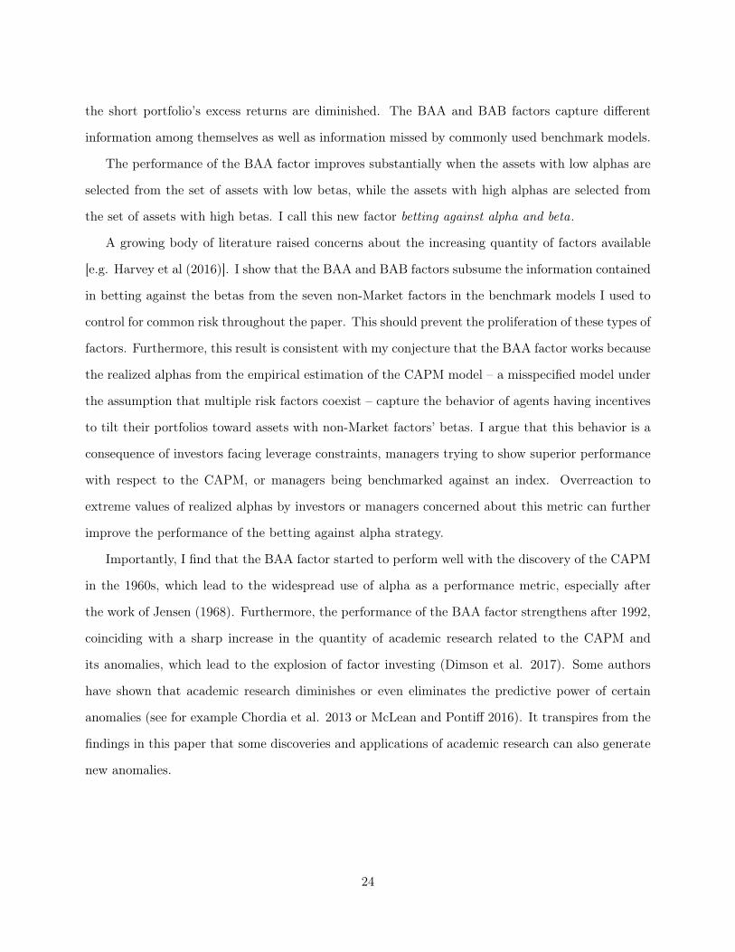
factor’s cumulative abnormal returns (CAR) generated from the 1930s until 1965 are negligible, (ii)
the CAPM era (1965-1992): the BAA factor consistently generated positive abnormal returns, and
(iii) the Smart Beta era (1993 onward): the growth rate of the CAR series generated by the BAA
factor has further increased with respect to the previous era. This can be clearly seen in Figure 1,
which depicts the monthly CAR of the BAA factor when regressed onto the empirical CAPM using
a 5-year rolling regression starting in January 1932 and finishing in December 2015. The dotted line
shows the trend of the CAR series within each era.
[Insert Figure 1 around here]
Note that the Smart Beta era coincides with the expansion of factor investing as a method for
portfolio allocation, for which the Fama and French (1992, 1993) and Jegadeesh and Titman (1993)
seminal papers undoubtedly played an important role (Dimson et al. 2017).7
Interestingly, I calculate the yearly number of academic works containing the phrase “Capital
Asset Pricing Model” and find that it shows similar patterns to that of the BAA factor’s CAR.
Furthermore, I find that after 1992 there is a sharp increase in the yearly quantities of academic
work produced containing the following three phrases: (i) Capital Asset Pricing Model , (ii) Arbitrage
Pricing Theory , and (iii) Capital Asset Pricing Model plus either the words Anomaly or Anomalies.
It seems that the more research that the CAPM model (and its anomalies) attracts, the faster
the growth in the CAR series of the BAA factor. Chordia et al. (2013) and McLean and Pontiff
(2016) showed that academic research diminishes or even eliminates the predictive power of certain
anomalies. My results suggest that academic research might also stem new ones.
Aside from the BAA factor, I also propose a second long-short strategy, which I call betting against
alpha and beta (BAAB). The motivation for BAAB follows immediately from the motivation of the
BAA factor. If certain investors tilt their portfolios toward assets with high realized MKT betas
and also toward assets with high realized alphas, then a portfolio consisting of high realized alpha
assets from the set of high realized MKT beta ones should be even more overpriced. A similar logic7There is an upward trend in the CAR series between 1942 and 1953. This trend disappears if we augment the
empirical CAPM with the HML factor, suggesting that assets with a high HML beta might have been overvaluedin that period. This is consistent with my assumptions and the fact that the value-premium was known before thedevelopment of the CAPM (e.g., Graham and Dodd 1934).
5

follows for the long position used to construct the BAAB factor that comprises the portfolio of low
realized alpha assets from the set of assets with low realized MKT betas.
The BAA, BAB, and BAAB factors are constructed using leverage, although I show in the paper
that the BAA factor also works as a standard long-short strategy without leverage. More precisely, to
compare across strategies, I developed a benchmark scenario in which I use the same weights for the
low and high portfolios of every levered strategy. The common weights are calculated following the
methodology developed in FP for the construction of their BAB factor. In the benchmark scenario,
I rebalance all strategies once a year. The monthly Sharpe Ratios of the BAA, BAB, and BAAB
factors are 0.22, 0.26, and 0.30, respectively.8 These monthly Sharpe Ratios are quite high when
compared to those of the factors in the benchmark models. For example, the monthly Sharpe Ratio
for the MKT factor during the same period is 0.11. The new BAA and BAAB factors are not priced
by the CAPM, Carhart, FF6 (FF5+Momentum), or FF6+Rev (FF6+Long-term reversal+Short-
term reversal) models. They generate monthly abnormal returns of around 1% between January
1973 and December 2015 with t-stats surpassing the hurdle of 3.0 suggested in Harvey et al. (2016).
Given the proliferation of factors in the literature, it is important to avoid the multiplication of
“betting against” any factor betas. According to equation (2) the BAA factor should capture the
information on betting against Smart beta factors. Therefore, the BAA and BAB factors should
summarize the information about betting against most factor’s beta strategies. Consistent with
this conjecture, I show that the BAB and BAA factors price the betting against beta strategies
calculated using the betas from the seven Smart Beta factors in the FF6 model augmented with the
Long-Term and Short-Term reversal factors.
In a related paper, Horenstein (2018) finds that using estimated alphas to evaluate strategies
constructed with leverage might lead to false positives too often. Therefore, in this paper I also use
rank estimation methods to test whether the proposed factors capture relevant information in the
cross-section of stocks returns. My results show that the BAA and BAB strategies capture different
information among themselves. The results also suggest that the BAA and BAB strategies capture
relevant information missed by the factors in the benchmark models.
The rest of the paper is organized as follows. Section 2 presents the data and elaborates on the8To avoid aggregation issues, I do not annualize the estimated monthly Sharpe Ratios [see Lo (2002)].
6

construction of the weights used to construct the factors with leverage. Section 3 presents the main
quantitative results. I conclude in Section 4. The Appendix presents additional robustness checks.
2 Data and construction of the levered strategies
2.1 Data
I use data on US individual stock returns from the Center for Research in Security Prices (CRSP)
from January 1927 until December 2015. The returns include dividends and correspond to common
stocks traded on the NYSE, NASDAQ, and AMEX, excluding REITs and ADRs. Data on the factors
used in the benchmark models are from Kenneth French’s website.9 The benchmark models are the
CAPM, Carhart model (1997), Fama-French Six Factor model (FF6, 2018), and FF6 augmented
with reversal factors (FF6+REV). The CAPM contains only the Market factor (the return on the
CRSP value-weighted portfolio minus the return on the 1-month Treasury bill). The Carhart model
augments the CAPM with the Small Minus Big factor (SMB), High Minus Low factor (HML), and
the Momentum factor (MOM, consists of selling losers and buying winners from the prior 6 to 12
months). The FF6 model augments Carhart’s model with the Robust Minus Weak (RMW) and
Conservative Minus Aggressive (CMA) factors.10 The FF6+REV model augments FF6 with the
Long-term reversal factor (LTR, consists of buying losers and selling winners from the prior 13 to
60 months) and the Short-term reversal factor (STR, consists of buying losers and selling winners
from the prior month).
2.2 Construction of the Betting Against Alpha, Betting Against Beta, and Bet-
ting Against Alpha and Beta factors
The Betting Against Beta (BAB) factor developed by Frazzini and Pedersen (FP, 2014) consists of
selling a portfolio made of high beta stocks’ excess returns over the risk free asset and buying a
portfolio made of low beta stocks’ excess returns (note that the long and short portfolios are both
zero-net investments). Additionally, both portfolios are scaled by the inverse of the risky assets’9http://mba.tuck.dartmouth.edu/pages/faculty/ken.french/data_library.html
10For a detailed explanation on how SMB, HML, RMW, and CMA are constructed, please see Fama and French(2015).
7
weighted betas, and thus, given that the average Market beta value fluctuates around one, the
excess returns of the low beta portfolio are amplified, while the excess returns of the high beta
portfolio are reduced.
The Betting Against Alpha (BAA) factor consists of selling a portfolio containing assets with
realized alphas bigger then the median alpha and buying a portfolio of assets with realized alphas
lower than the median alpha. The Betting Against Alpha and Beta (BAAB) factor also sells a
portfolio containing assets with high realized alphas and buys a portfolio containing assets with low
realized alphas. The difference between the BAA factor and the BAAB factor is that for the latter,
I first divide the sample into two groups: Assets with realized betas less than the median beta
and those with realized betas higher than the median beta. Then, using the sample of assets with
realized betas lower than the median beta, I create the long portfolio with assets having realized
alphas lower than the median alpha within that sample. Similarly, from the sample of assets with
realized betas higher than the median beta, I create the short portfolio with assets having realized
alphas larger than the median alpha within the high beta sample.
To simplify the comparison between the BAA, BAB, and BAAB factors, I will use the same
weights for the low and high portfolios in all of them. Therefore, I first construct the common
weights and then apply those weights to all factors’ short and long portfolios.
To calculate the common weight, I follow closely the methodology developed in FP. For each
asset i, βi = ρiM (σi/σM ), where ρiM is the correlation between the i asset’s returns and the Market
returns, while σi and σM are the asset i and Market estimated volatilities, respectively. As in FP,
the ρiM is estimated using five year data while σi and σM are estimated using yearly data. The
final Market beta assigned to an asset i (βMi ) is compressed towards one as in FP using the formula
βMi = 0.6βi + 0.4.
The βMi s lower (higher) than the median are assigned to the low (high) beta portfolio and
weighted using the same formula as in FP. More precisely, let nl be the number of assets in the
low beta portfolio and zl be the nl × 1 vector of beta ranks such that zli = rank(βMi ). The weight
of an asset i in the low beta portfolio is given by wli = (nl − zli + 1)/∑zli. Similarly, let nh be
the number of assets in the high beta portfolio and zh be the nh × 1 vector of beta ranks in this
8

portfolio, where zhi = rank(βMi ). The weight of an asset i in the high beta portfolio is given by
whi = zhi/∑zhi. Note that
∑wli =
∑whi = 1. The final weighted Market betas of the low and
high beta portfolios are βL =∑wliβ
Mi and βH =
∑whiβ
Mi respectively.
The main difference between this paper’s calculation of the weights βL and βH and the ones used
in FP is that they use daily data to estimate betas and I use monthly data. Additionally, they allow
for assets to have at least three years of data in their calculation, while I use assets with five years of
data. On average, this paper’s weights imply an investment of around $1.67 in the long portfolio and
$0.63 in the short portfolio using yearly rebalanced strategies (end of December). For robustness, I
also use 1-month, 6-month, 24-month, and 48-month rebalancing periods in the calculations.
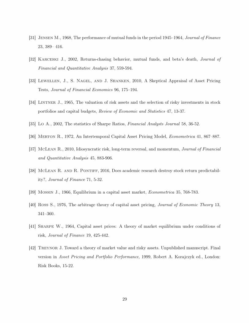
Figure 2 below shows the weights, 1βLtand 1
βHt, calculated with my modified technique rebalancing
every twelve months and the monthly weights calculated with the FP method (using daily data
available for at least 36 and up to 60 months and rebalancing monthly) for the period of January
1973 - December 2015. It can be observed that both sets of weights show a similar pattern between
1973 and 2015. The main difference is that my modification creates a slightly larger spread between
the low beta and high beta portfolios’ weights. However, since I apply the same weights to all
strategies, this difference in the weights’ spread does not modify the qualitative results of this paper.
[Insert Figure 2 around here]
Once I have calculated the common weights βL and βH , then I am ready to calculate the BAB,
BAA, and BAAB factors. To assign assets to the low and high portfolios I will use the estimated
parameters from the CAPM model using the most common time span and frequency observed in
the literature: 5 years of monthly data (e.g., Black et al. 1972; Banz 1981; Fama-French 1992, 1993,
2015, 2018). As discussed in the calculation of the common weights, FP suggests estimating the
Market betas differently than using traditional regression methods. However, my goal is not to find
the highest possible Sharpe Ratio but to construct a benchmark scenario that allows me to compare
across strategies. Therefore, using the same estimation methods across strategies to calculate the
parameters of interest seems appropriate for this paper.11
The returns of the low and high portfolio are rL =∑wlir
Li and rH =
∑whir
Hi , respectively.
11Results for the BAB factor are qualitatively the same if I rank assets using FP’s methodology to calculate beta.
9
However, now the ranks zli and zhi are calculated with the estimated values of beta and alpha from
the CAPM regression. The BAB factor’s return rebalanced monthly and consisting of selling the
high beta portfolio and buying the low beta portfolio is rBABt+1 = 1βLt(rLt+1 − rft+1)− 1
βHt(rHt+1 − rft+1).
In the case of yearly rebalancing at the end of December, the BAB factor’s return is rBABt+s =
1βLt(rLt+s − rft+s) − 1
βHt(rHt+s − rft+s), where s = 1, ..., 12 and t corresponds to December. The same
weights βL and βH apply to the BAA and BAAB factors. The only difference is that for the BAA
and BAAB factors, zli = rank(α̂Li ) and zhi = rank(α̂Hi ), where α̂Li and α̂Hi are alphas below and
above the median alpha, respectively.
3 Results
3.1 Betting against alpha across time
I start the empirical analysis by studying the performance of the BAA factor during the three eras
described in the Introduction. In this Section, I will also relate the BAA factor’s performance to the
popularity of the CAPM literature, which I propose to measure by the yearly quantity of scientific
output related to it.
The BAA factor in this Section is constructed using a sample starting in 1927 and using the
following benchmark scenario: (i) The holding period return for the BAA factor is 12 months, where
betas and alphas are estimated at the end of December. Then, portfolios are formed on the first
trading day of January and maintained for 12 months until the last trading day of December. (ii)
Portfolios are formed using the entire universe of the CRSP database as explained in Section 2.1.12
(iii) The alphas used for assigning assets to the short and long portfolios of the BAA factor are
estimated using the standard CAPM.13 (iv) The period of analysis is 1927-2015; thus, the BAA
factor spans the 1932-2015 period since the first five years of data are needed for estimating the
initial realized alphas.
Figure 1 in the Introduction shows the monthly cumulative abnormal returns (CAR) of the BAA12The CRSP database experienced two expansions during this period. The AMEX data was incorporated in 1962
and the NASDAQ data in 1972. Restricting the analysis of this Section to using only NYSE data does not changethe results qualitatively.
13The betas used to construct the weights of the long-short strategies are estimated using FP’s methodology. Formore information please see Section 2.2.
10
factor when regressed against the Market factor using a 5-year rolling regression starting in January
1932 and finishing in December 2015. It shows the three distinguishable periods: (i) The Pre-CAPM
era (1937-1964), (ii) The CAPM era (1965-1992), and (iii) the Smart Beta era (1993 onward).
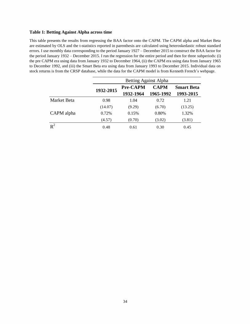
The results in Figure 1 can be further supported with those in Table 1 below. The table shows
the estimated Market betas and CAPM alphas of the BAA factor for the entire period 1932-2015
and the three aforementioned eras.
[Insert Table 1 around here]
The CAPM’s abnormal return generated by the BAA factor for the entire period of 1932-2015
is 0.72% monthly and statistically significant (t-stat of 4.57). However, once we analyzed the three
eras separately, the CAPM alpha generated by the BAA factor is insignificant for the pre-CAPM
era, while it is statistically significant (t-stat of 3.02) and economically meaningful (0.80% monthly)
for the CAPM era. The magnitude of the CAPM alpha generated by the BAA factor increases by
more than 50% – to 1.32% monthly – in the Smart Beta era with respect to the previous era (with
a t-stat of 3.81).
The beginning of the CAPM era coincides with the theoretical development of the model in
the mid-1960s.14 At the same point, the starting point of the Smart Beta era coincides with the
publication of the seminal papers by Fama and French (1992, 1993) and Jeegadesh and Titman
(1993), which lead to a substantial expansion in the research for new Smart Beta factors as well
as to an expansion in the application of factor investing in the practitioners’ world (Dimson et al.
2017).
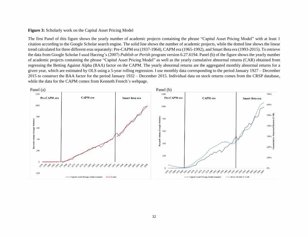
Now I will show that the performance of the BAA factor can be linked to the popularity of
the CAPM in the academic literature, which undoubtedly migrated to the practitioners’ world as it
became the benchmark model to evaluate fund managers’ performances (e.g., Jensen 1968, Baker et
al. 2011, Barber et al. 2016). To capture the popularity of the CAPM in the academic literature,
I counted the yearly number of scholarly works produced that contain the phrase “Capital Asset
Pricing Model” between 1956 and 2008 using the Google Scholar search engine.15 I restricted the
sample to academic works having at least one citation according to the search engine. Panel (a) of14See Footnote #6.15See Appendix C for a detailed explanation on how the calculations were done.
11

Figure 3 shows the yearly number of works containing this phrase (solid line) as well as a linear trend
calculated separately for the three different eras (dotted line). For comparison purposes, Panel (b)
shows again the evolution of the yearly number of academic works containing the phrase “Capital
Asset Pricing Model” together with the yearly CAR of the BAA factor.
[Insert Figure 3 around here]
Panel (a) shows that during the CAPM era (1965-1992) the yearly number of new works with at
least one citation containing the phrase “Capital Asset Pricing Models” increased from 4 to 484. By
2008 that number reached almost 1000. The figure’s Panel (b) shows that the series of BAA CAR
mimics the variable I use to capture the popularity of the CAPM’s literature. It is also relevant
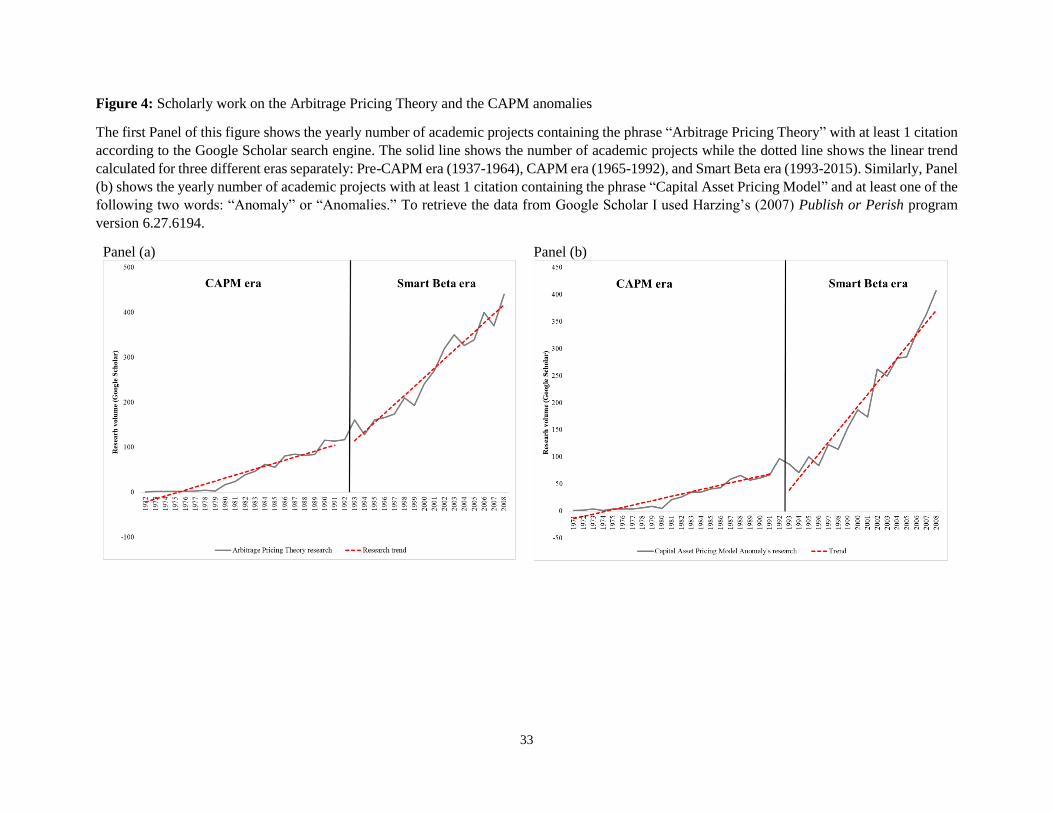
to analyze the popularity of the multifactor asset pricing model’s literature, which supports the
existence of Smart Beta factors.16 Therefore, in Panel (a) of Figure 4 I plot the number of scholarly
works with at least one citation in Google Scholar when searching for the phrase “Arbitrage Pricing
Theory,” as well as its trend. Unsurprisingly, the number starts to increase after the publication of
Ross’s seminal paper in 1976. As with the CAPM case, the trend becomes much steeper during the
Smart Beta era. A similar pattern can be observed when searching for academic works with the
phrase “Capital Asset Pricing Model” with the added condition that at least one of the following two
words should also appear in the publication: “Anomaly” or “Anomalies.” The results are shown in
Panel (b) of Figure 4. Between 1980 and 1992 the number of yearly works produced containing these
words increased from 5 to 97. By the year 2008 there were already 407 produced yearly. Again, the
upward trend appears during the CAPM era and becomes much steeper during the Smart Beta era.
[Insert Figure 4 around here]
Overall, these results suggest that academic research can have a non-negligible impact on the
financial markets in a way not documented before. Previous work showed that academic research
reduces or even eliminates the predictive power of certain anomalies (see for example Chordia et al.
2013 or McLean and Pontiff 2016). My results suggest that academic research can also originate
new anomalies.16See Footnote #2.
12

3.2 Analysis of the factors’ performances after the development of the CAPM
I now study the performance metrics of the BAA and BAAB factors under the benchmark scenario
described in Section 3.1, but focusing on the relevant period of analysis, the time period starting
with the CAPM era when alpha was suggested as a performance metric (Jensen 1968). Therefore,
in this Section I use the same benchmark scenario as in the previous one, except that the period of
analysis is 1973-2015; thus, I use data from 1968-2015 since the first five years of data are needed
for estimating the initial realized alphas and betas. Section 3.5 and Section 3.6 contain results for
the factors’ performance metrics across different ranges of market capitalization values for the data
and different holding periods for the strategies. In Appendix A, I present results for the factors
constructed using alphas estimated from the Carhart, FF6, and FF6+Rev models.
Table 2 shows the summary statistics for the low portfolio, high portfolio, and the low minus high
portfolio strategy with leverage. I added to the table the BAB factor for comparison purposes. I
report the monthly Sharpe Ratios17, average monthly excess return, monthly CAPM alpha, monthly
Carhart alpha, monthly FF6 alpha, monthly FF6+Rev alpha, and average market capitalization
value of the weighted portfolios in thousands of 2010 US dollars (Size) at the time of rebalancing.
Heteroskedastic robust t-statistics are in parenthesis below each model’s estimated alphas.
[Insert Table 2 around here]
The first line of Table 2 shows that the Sharpe Ratio decreases for both strategies when we move
from the low to the high portfolio. The BAB factor’s monthly Sharpe Ratio is 0.26 while the BAA
one is 0.22. Both factors have a higher monthly Sharpe Ratio than the Market (0.11), SMB (0.07),
HML (0.12), RMW (0.11), CMA (0.17), MOM (0.16), LTR (0.10), and STR (0.13) factors.
The BAA factor produces abnormal returns across all models used to control for systematic
risk, with t-statistics easily surpassing the hurdle of 3.0 suggested by Harvey et al. (2016). The
abnormal returns of the BAA factor are usually bigger than those of the BAB one; however, this
should not be considered an outperformance of the BAA factor since the original BAB factor of FP
is constructed with daily data and monthly rebalancing of the long-short strategy’s portfolios, while17See Footnote #8.
13

in this benchmark scenario I use monthly data and yearly rebalancing.18 As I stressed in Section
2.2, the goal of this paper is not to find the factor with the highest Sharpe Ratio but to document
and analyze the relevance and characteristics of the strategies developed in this paper. Finally, the
BAA low portfolio is comprised on average of smaller market cap stocks than those of the BAB low
portfolio, while the BAA high portfolio is comprised of larger market cap stocks than those of the
BAB high portfolio. Therefore, size might affect the BAA factor more than the BAB one. We will
come back to this issue later in Section 3.5.
As I argue in the introduction, assets with high realized alphas from the sample of assets with
high realized betas should be the most overpriced, while those with low alphas from the sample of
low beta assets should be the most underpriced. Before moving to the results for the BAAB factor,
I first check if betting against alpha works across different values of Market betas. Table 3 presents
the same performance metrics as before for the low alpha portfolio, high alpha portfolio, and levered
low-high portfolio strategy. However, in this table I calculate those metrics for the subset of assets
with betas above the median beta (High Beta) and for the subset of assets with betas below the
median beta (Low Beta) separately.
[Insert Table 3 around here]
Table 3 shows that Sharpe Ratios and abnormal returns across all models decrease as alpha
increases for the low and high beta portfolios. Consistent with this paper’s conjecture, the high
alpha portfolio constructed from high beta assets has the lowest Sharpe Ratio, while the low alpha
portfolio constructed from low beta assets has the highest one. As expected, Sharpe Ratios decrease
as beta increases. The BAAB factor shorts the high alpha assets of the high beta portfolio and
buys the low alpha assets of the low beta portfolio.19 Table 4 shows that the monthly Sharpe Ratio
of the BAAB strategy surpasses that of the BAA and BAB factors alone and almost triples that
of the Market factor. Monthly abnormal returns are around 1% and statistically significant for all
benchmark models.18In Section 3.6 below I show that the performance of the BAB factor improves when the rebalancing frequency
decreases.19One important difference between the combined strategy with respect to the single-sorted one is that the combined
uses around 50% of the CRSP cleaned database, while the single sorted one uses 100%.
14

[Insert Table 4 around here]
I now analyze the correlation between the factors constructed with leverage and the factors used
to control for systematic risk in this paper (Market, SMB, HML, RMW, CMA, MOM, LTR, and
STR factors). Results are shown in Table 5.
[Insert Table 5 around here]
The Pearson’s correlation coefficient (henceforth correlation) between the BAA and BAB factors
is quite low, only 0.21, which implies that betting against alpha is probably not the same as betting
against beta. This issue is studied in more depth in Section 3.3. The correlation between the BAA
factor and the FF6+Rev factors is larger than that of the BAB factor and the FF6+Rev factors,
especially the one between the BAA factor and the Market factor (0.61). Once the BAA factor is
combined with the BAB one into the BAAB factor, the correlation between the BAAB factor and
the FF6 factors decreases. For example, the correlation between the BAAB factor and the Market
factor is just 0.32, and no correlation with any other FF6+Rev factor surpasses 0.4 except for that
with LTR (0.51).20 Additionally, the BAAB factor still has a relatively high correlation with the
BAA factor (0.82) and a relatively lower correlation with the BAB factor (0.55).
Finally, Table 6 presents performance metrics for the dataset divided into decile portfolios sorted
on realized CAPM alphas in Panel (a) and on realized CAPM betas in Panel (b). Assets within
each portfolio are equally-weighted.
[Insert Table 6 around here]
The first line of both panels shows that Sharpe Ratios are decreasing in both realized alphas and
realized betas. However, the second line shows that excess returns are decreasing in realized alphas
while they slightly increase in realized betas. The last column of the table shows the results from
using a low minus high strategy without leverage corresponding to using only the highest and lowest20It should not be surprising that the BAA and BAAB factors have a relatively high correlation with the LTR factor.
This can be easily seen by analyzing the fitted equation from the estimated CAPM model µ̄i = α̂i + β̂i × µ̄Market,where µ̄i is the average excess return over rf for asset i and µ̄Market is the Market portfolio’s average risk premium.While LTR consists of sorting assets based on µ̄i, BAA consists of sorting assets on α̂i and BAAB consists of sortingassets on α̂i and β̂i.
15
decile portfolios.21 The first six lines of the Low-High column in Panel (a) show that betting against
alpha, in principle, works without leverage. However, since the BAAB factor requires combining the
BAA factor with the BAB factor and one of the reasons discussed in the Introduction for the BAA
factor to work is the existence of liquidity constrained investors, then it is natural to construct all
strategies using leverage.
As expected, the ninth line in Panel (a) shows that Average Realized CAPM Alpha increase for
portfolios sorted by this variable, while the tenth line of Panel (b) shows the same for portfolios
sorted by Average Realized Market Beta. The prediction of FP still holds: A low realized beta
implies a future high alpha, while a high realized beta implies a future low alpha. My prediction
also holds: A low realized alpha implies a future high alpha, while a high realized alpha implies a
future low alpha. This can be seen in lines three to six of Panel (a) and Panel (b), where I present
the abnormal returns for the CAPM, Carhart, FF6, and FF6+Rev models.
Lines seven and eight in Panel (b) show that the Average Total Volatility and the Average
Idiosyncratic Volatility of the assets in the portfolios increase with the average realized beta [see for
example Baker et al. (2011)]. Importantly, Panel (a) shows that the relationship between realized
alphas and volatility presents a U-shape, suggesting that betting against alpha is not related to the
low-volatility anomaly. The relationship between realized alpha and realized beta is also U-shaped
as shown in lines nine and ten of Panel (a) and Panel (b). This further suggests that betting against
alpha is not the same as betting against beta.
To further study the relationship between the beta, alpha, and volatility patterns, I created
two more strategies: A betting against total volatility strategy and a betting against idiosyncratic
volatility strategy. Details about the performance metrics of these strategies are in Appendix B.
The correlation coefficients of these two volatility strategies with respect to the BAB factor are 0.56
and 0.51, respectively, while their correlations with respect to the BAA factor are -0.18 and -0.12,
respectively. Overall, the low-volatility anomaly does not seem related to betting against alpha.
Finally, the last line of Panel (a) shows that the relationship between market capitalization
(Size) and Average Realized CAPM Alpha has an inverted U-shape. The last line of Panel (b) shows21Note that here the strategies use only the largest and smallest decile portfolios (20% of the available stocks), while
the results presented in the previous tables use much more data (50% of the available stocks for the BAAB factor and100% for the BAA and BAB factors).
16

that this inverted U-shape is even more pronounced for the relationship between Size and Average
Realized Market Beta. Thus, as confirmed in Section 3.5 below, removing small stocks from the
sample negatively impacts the performance metrics of the factors since it is equivalent to removing
assets from both extreme decile portfolios. Additionally, this inverted U-shape between market
capitalization and realize alpha (and beta) implies that using value-weighted portfolios to construct
these strategies should have a negative impact on their performance metrics too: While the BAA,
BAB, and BAAB factors are constructed overweighting the assets in the extreme range of the alpha
and beta values, a value-weighted version of these strategies will overweight the assets in the middle
of the range. Thus, a strategy constructed using value-weighted portfolios will overweight alphas
close to zero and betas close to one. Overweighting such assets is exactly the opposite of what these
strategies require.22
3.3 BAB and BAA factors as a new source of stock returns’ comovement
In the previous sections I showed that the BAA factor is not priced by either the CAPM, Carhart,
FF6, or FF6+Rev models. Additionally, and not shown in this paper, I found that the BAA factor
cannot price the BAB factor and vice-versa.23 However, that a factor generates significant pricing
errors when regressed against other factors is not sufficient evidence about that factor capturing a
missing dimension in the space of stock returns. For example, using rank estimation methods, Ahn
et al. (2017) found that 26 commonly used factors capture at most five independent vectors in the
space of stock returns. Importantly, Horenstein (2018) finds that when regressing tradeable factors
constructed with leverage on tradeable factors without leverage, econometricians will find highly
statistically significant pricing errors too often.
Therefore, an important question that remains to be answered is whether the BAA and BAB
strategies capture different information about the comovement of stock returns, as well as information22As explained in this paragraph, using value-weighted or any other type of weights violates the strategies’ premises
of overweighting low alpha (beta) assets in the low alpha (beta) portfolio, while underweighting this type of asset in thehigh alpha (beta) portfolio. Thus, results with equally-weighted (or value-weighted) portfolios should be consideredof second order importance. Studying the impact of size across strategies is of paramount importance, but shouldbe performed taking into account the strategies’ premises. This can be done by studying the performance of thestrategies across sets of assets belonging to different market capitalization ranges. The latter is the objective ofSection 3.5 below.
23Results are available upon request.
17

missed by the FF6 and reversal factors. A natural way to answer this question is to estimate the
rank of the beta matrix generated by these strategies when they are used as regressors. As Ahn
et al. (2017) point out, “the rank of the beta matrix corresponding to a set of factors equals the
number of factors whose prices are identifiable.” In other words, the rank of the beta matrix will tell
us the number of different sources of stock returns’ comovement captured by a set of factors.
First I will test whether the BAA and BAB factors produce a full rank beta matrix when used
together as regressors. This will allow me to assess whether they are capturing different information.
Then, I will use these factors to augment the CAPM, Carhart, FF6, and FF6+Rev models to analyze
if the BAA and BAB factors contain information missed by any of these empirical models.
As the tests’ response variables, I will use portfolio returns.24 Following the suggestion of
Lewellen et al. (2010), I consider the combined set of the 25 Size and Book to Market portfo-
lios with the 30 Industrial portfolios.
While many alternative rank estimators are available in the literature, they are designed for the
analysis of data with a small number of cross section units (N ). Consequently, they may not be
appropriate for the estimation of the beta matrix with large N. Ahn et al. (2017), however, found
that a restricted version of the BIC (RBIC) rank estimator of Cragg and Donald (1997) has good
finite-sample properties if the return data used contains the time series observations of at least 240
months (T ≥ 240) over individual portfolios whose number does not exceed one half of the time
series observations (N ≤ T/2). My data fits the desirable properties for the RBIC rank estimator
since the time span is January 1973 - September 2015 (T = 516) and the number of cross-sectional
units is N = 55.
Table 7 presents the rank estimations’ results. Each row corresponds to a set of k factors used as
regressors to generate the estimated beta matrix (or matrix of factor loadings). Thus, k corresponds
to the maximum rank attainable by the beta matrix.
[Insert Table 7 around here]
The results in the first three lines correspond to using only the BAA and BAB factors. Both24Portfolio returns contain a stronger factor structure than individual stock returns. Ahn et al. (2017) show that
a higher signal to noise ratio of the factors with respect to the response variables increases the accuracy of their rankestimator.
18
strategies capture a relevant source of comovement according to the RBIC estimator (the estimated
rank equals 1 for the BAA and BAB factors separately). When the BAA and BAB factors are used
together, they generate a full rank beta matrix (the RBIC rank estimator equals 2), indicating that
the information they capture is different. I now move on to analyze if the BAA and BAB factors
capture a different source of comovement than the CAPM, Carhart, FF6, and FF6+Rev models.
Lines (v) and (vi) of Table 7 show that both factors augment the rank generated by the CAPM.
Thus, both strategies capture information missed by the Market factor. Line (vii) shows that when
both factors are added to the CAPM (k=3), the estimated rank of the beta matrix is 3, which
confirms my result that BAA and BAB capture different information among themselves. Similar
results are obtained when augmenting the Carhart model with the BAA and BAB strategies [lines
(viii) to (xi)]. Line (viii) shows that the Carhart model generates a rank deficient beta matrix (k=4
but the estimated rank is 3). The rank augments to 4 when adding either the BAA or BAB factor
and augments to 5 when adding both factors [lines (ix) to (xi)]. Finally, the FF6 and FF6+Rev
model also produces rank-deficient beta matrices [lines (xii) and (xvi)]. As with the Carhart model’s
case, both the BAA and BAB factors increase the rank of the beta matrix by one when added to
the models separately and by two when added together.
In summary, this Section shows that the BAA and BAB factors not only capture different
information among themselves but also with respect to the factor contained in the benchmark
models.
3.4 Betting against other factors’ betas
Recalling the discussion in the Introduction, previous research shows that, for example, liquidity
constraints [Frazzini and Pedersen (2014)] and benchmarking [Baker et al. (2011)] generate incentives
for mutual fund managers to tilt their portfolios toward assets with high Market betas. Then, I
argued that investors’ liquidity constraints, benchmarking, and investors’ inattention to Smart Beta
factors [Barber et al. (2016)] also generate incentives for mutual fund managers to tilt their portfolios
toward assets with a high Smart Beta factor betas. As shown by equation (2) in the Introduction,
assets’ Smart Beta factor betas times their corresponding factors’ risk premiums are reflected in the
19

estimated CAPM’s alpha if the true model includes multiple factors. Therefore, as I also argued
in the Introduction, the BAA and BAB factors should suffice to price the betting against Smart
Beta strategies. Thus, now I will analyze whether the BAA and BAB factors can price betting
against beta strategies constructed using the betas of the FF6+Rev factors used to augment the
CAPM (SMB, HML, CMA, RMW, MOM, LTR, and STR). Each factor’s betas are estimated using
single-factor regressions.
First, Table 8 shows the summary statistics for these strategies’ performance metrics. I use the
same weights for the long and short portfolios as I did for the BAB and BAA factors before. The
long and short portfolios are rebalanced every December.
[Insert Table 8 around here]
Panel (a) and Panel (e) show that betting against the SMB beta and betting against the MOM
beta strategies produce high monthly Sharpe Ratios (0.20 and 0.19, respectively) and significant
abnormal returns. Betting against the betas generated by HML, CMA, RMW, LTR, and STR does
not produce high Sharpe Ratios. In fact, the Sharpe Ratios do not even decrease as we move from
the low to the high portfolio. However, all the strategies seem to produce statistically significant
alphas with respect to some of the benchmark models.
Let me now move to the main objective of this Section, which is to assess whether the BAA
and BAB factors suffice to price the levered strategies constructed with the Smart Beta factors,
especially those using the betas corresponding to SMB and MOM, which produce non-negligible
performance metrics. To answer this question I use an insight from Barillas and Shanken (2017).
They showed that “it turns out that test assets tell us nothing about model comparison, beyond
what we learn by examining the extent to which each model prices the factors in the other models.”
In other words, to compare factor models based on estimated pricing errors, we can simply regress
one factor against another set of factors and see if the pricing error is statistically significant. If it
is not, then the factor used as a dependent variable cannot improve over a model containing the
factors used as regressors. For this purpose, I run regressions using the betting against Smart Beta
strategies presented in Table 8 as dependent variables and the BAA and BAB factors as regressors.25
25Horenstein (2018) finds that tradeable factors constructed using leverage like the one studied in this paper produce
20

Results are presented in Table 9.
[Insert Table 9 around here]
Looking at the intercepts, observe that the BAA and BAB factors price all the other strategies
of interest. Therefore, my conjecture about the BAA and BAB factors subsuming the pricing
information of other betting against beta strategies is supported by the data.
3.5 BAA, BAB, and BAAB factors across size
Most long-short strategies that produce abnormal returns show decreasing performance as companies
with low market capitalization values are removed from the sample [e.g., Fama and French (2008)].
In fact, the positive risk premiums generated by many factors disappear once the small companies
(or even micro cap companies) are removed from the sample. Therefore, it is important to study
the performance of the BAA, BAB, and BAAB factors for different levels of market cap.
Before performing the analysis separating companies by market capitalization, it is important
to remember that the relationship between size and realized alpha, as well as that between size
and realized beta, has an inverted U-shape form.26 This mean that there are small stocks at both
extremes of the alpha and beta ranges. Thus, removing small stocks will negatively affect the BAA,
BAB, and BAAB factors’ performance metrics.
Using the NYSE 30th and 70th percentile for market capitalization cutoff values, every December,
I divide the dataset into three categories: (i) 30% Small, which contains all firms whose market cap
is equal to or below the 30th percentile; (ii) 40% Medium, which contains all firms whose market
cap is greater than the 30th percentile and lower than or equal to the 70th percentile; and (iii) 30%
Big, which contains those firms with a market cap value greater than the 70th percentile. For each
group, I construct the BAA, BAB, and BAAB factors and run the same performance metrics as
before. As in the benchmark scenario, all strategies use a 12-month holding period.27 Results are
presented in Table 10.
positive and statistically significant abnormal returns too often when regressed against tradeable factors withoutleverage. He also finds that this problem disappears once tradeable factors constructed with leverage are regressedonto other tradeable factors constructed using the same leverage, which inspired this Section of the paper.
26See Table 6 in Section 3.2 and the corresponding discussion in the last paragraph of that section.27Results improve for the BAA and BAAB factors when using a 24-month holding period and for the BAB factor
when using a 1-month holding period.
21

[Insert Table 10 around here]
Sharpe Ratios decrease as the market capitalization value of the companies used to construct
the strategies increases. However, an important desirable property is maintained: For the three
strategies, the Sharpe Ratio of the low portfolio surpasses that of the large one across all size
groups. When looking at average returns, all strategies produce positive risk premiums across size
groups too. In the case of the BAA and BAAB strategies, the low portfolio generates higher average
returns than the high portfolio across all size groups.
The CAPM cannot price the factors constructed with any set of market capitalization clusters,
generating abnormal returns at the 1% level of significance or less across all groups. The only
exception is the BAA factor, which generates abnormal returns at the 5% level of significance or
less when large stocks are used. When controlling for the Carhart model, the results for the BAA
factor are quite similar to those obtained when controlling for the CAPM. The BAB factor presents
a different scenario: It only generates statistically significant abnormal returns when small stocks
are used. The BAA and BAAB factors lose some power when controlling for the Carhart model,
generating statistically significant abnormal returns at the 1% level or less only for the small and
medium group, while for the group of large stocks the abnormal returns are significant at the 5%
level. Finally, when I control for the FF6 or FF6+Rev model, the BAB and BAAB strategies
only generate abnormal returns when small cap assets are used. The BAA factor still generates
statistically significant abnormal returns for the 40% Medium group, but no strategy generates
significant abnormal returns for the 30% Big one.
Overall, I find that the analyzed strategies maintain some desirable properties across all size
groups, like decreasing Sharpe Ratios across portfolios and positive risk premiums. As I include
more factors in the empirical asset pricing model used to test the strategies, abnormal returns
for strategies using only large stocks diminish and for the FF6 and FF6+Rev models disappear.
However, Sharpe Ratios and risk premiums are still large. For example, when using the 30% biggest
stocks, the BAAB factor generates a monthly risk premium of almost 1% and a monthly Sharpe
Ratio of 0.18, which is 65% larger than that of the Market factor and surpasses that of any of the
22

factors in the benchmark models.28
3.6 BAA, BAB, and BAAB factors for different holding periods
In this Section I analyze the performance of the different strategies when rebalancing them every
1-month, 6-month, 12-month (benchmark scenario), 24-month, and 48-month periods. As in the
previous Section, I use the same weights for every strategy, where I recalculate the weights at the
end of each holding period using the formulas presented in Section 2.2.
Table 11 presents the performance metrics across holding period returns for the BAA, BAB, and
BAAB factors.
[Insert Table 11 around here]
The BAA and BAAB factors show their best performances when rebalancing portfolios every
24 months. In the case of the BAAB factor, its Sharpe Ratio increases to 0.34, which is more than
three times larger than that of the Market factor.
For the BAB factor, Sharpe Ratios and abnormal returns decrease when augmenting the holding
period of the strategy. For this factor, the highest Sharpe Ratio, average returns, and abnormal
returns are observed when the strategy is rebalanced monthly as suggested in FP.
4 Concluding remarks
I find that selling assets having high realized CAPM alphas and buying assets having low realized
CAPM alphas leads to positive future returns, positive and statistically significant abnormal returns,
and high Sharpe Ratios.
To capture these patterns, I propose a long-short strategy I called betting against alpha (BAA)
that produces sizable Sharpe Ratios, risk premiums, and abnormal returns. Following Frazzini and
Pedersen’s (2014) construction of their betting against beta (BAB) factor, the BAA factor is a zero-
net investment strategy with leverage, where the long portfolio’s excess returns are magnified and28For the 1972-2015 period, the monthly Sharpe Ratios of the other factors are 0.11 for the Market Portfolio, 0.07
for SMB, 0.12 for HML, 0.11 for RMW, 0.17 for CMA, 0.16 for MOM, 0.10 for LTR, and 0.13 for STR.
23
the short portfolio’s excess returns are diminished. The BAA and BAB factors capture different
information among themselves as well as information missed by commonly used benchmark models.
The performance of the BAA factor improves substantially when the assets with low alphas are
selected from the set of assets with low betas, while the assets with high alphas are selected from
the set of assets with high betas. I call this new factor betting against alpha and beta.
A growing body of literature raised concerns about the increasing quantity of factors available
[e.g. Harvey et al (2016)]. I show that the BAA and BAB factors subsume the information contained
in betting against the betas from the seven non-Market factors in the benchmark models I used to
control for common risk throughout the paper. This should prevent the proliferation of these types of
factors. Furthermore, this result is consistent with my conjecture that the BAA factor works because
the realized alphas from the empirical estimation of the CAPM model – a misspecified model under
the assumption that multiple risk factors coexist – capture the behavior of agents having incentives
to tilt their portfolios toward assets with non-Market factors’ betas. I argue that this behavior is a
consequence of investors facing leverage constraints, managers trying to show superior performance
with respect to the CAPM, or managers being benchmarked against an index. Overreaction to
extreme values of realized alphas by investors or managers concerned about this metric can further
improve the performance of the betting against alpha strategy.
Importantly, I find that the BAA factor started to perform well with the discovery of the CAPM
in the 1960s, which lead to the widespread use of alpha as a performance metric, especially after
the work of Jensen (1968). Furthermore, the performance of the BAA factor strengthens after 1992,
coinciding with a sharp increase in the quantity of academic research related to the CAPM and
its anomalies, which lead to the explosion of factor investing (Dimson et al. 2017). Some authors
have shown that academic research diminishes or even eliminates the predictive power of certain
anomalies (see for example Chordia et al. 2013 or McLean and Pontiff 2016). It transpires from the
findings in this paper that some discoveries and applications of academic research can also generate
new anomalies.
24

Appendix: Robustness checks
A BAA strategies using Carhart, FF6, and FF6+Rev models’ alphas
In this Section I check that the main results still hold when the alphas for the BAA strategies are
calculated using either the Carhart, FF6, or FF6+Rev models. For the levered low minus high
strategies, I maintain the same weights used in the main body of the paper (see Section 2.2). Table
A1 replicates Table 2 in the paper for the Carhart, FF6, and FF6+Rev models. Overall, results are
similar.
[Insert Table A1 around here]
B Betting against idiosyncratic and total volatility
In this Section I present the performance metrics of two more “betting against” strategies mentioned
in the Introduction: (i) Betting Against Total Volatility (BATV) and (ii) Betting Against Idiosyn-
cratic Volatility (BAIV). These strategies are constructed using the same weight for the long and
short portfolios already used for the BAA, BAB, and BAAB factors. In the BATV strategy, assets
are sorted according to their realized variance during the 60 months prior to the sorting date. In
the BAIV strategy, assets are sorted according to their residual variance calculated from the CAPM
regression using data from 60 months prior to the sorting date. Results are presented in Table B1
below.
[Insert Table B1 around here]
Finally, Table B2 presents the correlation coefficients between the BAA, BAB, BAAB, BATV,
and BAIV strategies.
[Insert Table B2 around here]
C Construction of the citations’ indices
This Section describes the construction of the citation indices depicted in Figure 3 and Figure 4.
The source data is extracted from the Google Scholar search engine results using Harzing’s (2007)
25

program Publish or Perish version 6.27.6194. This program allowed me to create Excel spreadsheets
with the yearly outcomes from the Google Scholar search engine. In my calculations I only kept
those works having at least one citation in Google Scholar. Since Google Scholar limits the results
of any search to the 1000 most cited papers, I stopped my search when the yearly results show 1000
works with at least 1 citation. For the case when searching for the phrase “Capital Asset Pricing
Model,” this limit is reached in 2009. Therefore, I stopped the indices creation in 2008.
To calculate the number of academic works containing the phrase “Capital Asset Pricing Model”
presented in Figure 3, I search yearly this phrase starting in 1950. However, focusing on just this
phrase left out of the sample important works like Mossin (1966). This is because the name Capital
Asset Pricing Model became popular by the end of the 1960s. For this reason, I added to the sample
the results of searches for “Capital Asset Prices” between 1920 and 1975, while removing entries
already obtained when searching for “Capital Asset Pricing Model” to avoid double counting.
I followed a similar procedure to calculate the number of academic projects containing the phrase
“Arbitrage Pricing Theory” and the phrase “Capital Asset Pricing Model” plus either the word
“Anomaly” or “Anomalies.” For these two searches, the limit of 1000 results with at least one
citation in a year was never reached.
References
[1] Agarwal V., T. Green, and H. Ren, 2017, Alpha or beta in the eye of the beholder: What
drives hedge fund flows?, forthcoming Journal of Financial Economics.
[2] Ahn S., A. Horenstein, and N. Wang, 2018, Beta matrix and common factors in stock
returns, forthcoming Journal of Financial and Quantitative Analysis.
[3] Baker M., B. Bradley, and J. Wurgler, 2011, Benchmarks as limits to arbitrage: Un-
derstanding the low-volatility anomaly, Financial Analysts Journal 67, 40-54.
[4] Banz R., 1981, The relationship between return and market value of common stocks, Journal
of Financial Economics 9, 3-18.
26

[5] Barber B., X. Huang, and T. Odean, 2016, Which factors matter to investors? Evidence
from mutual fund flows, Review of Financial Studies 29, 2600-2642.
[6] Barillas F. and J. Shanken, 2017, Which alpha?, Review of Financial Studies 30, 1316-
1338.
[7] Black F., 1972, Capital market equilibrium with restricted borrowing, Journal of Business
45, 444-455.
[8] Black F., M. Jensen, and M. Scholes, 1972, The capital asset pricing model: Some
empirical tests, working paper available https://ssrn.com/abstract=908569
[9] Buffa A., D. Vayanos, and P. Woolley, 2017, Asset management contracts and equilib-
rium prices, working paper.
[10] Carhart M., 1997, On persistence in mutual fund performance, Journal of Finance 52, 57-82.
[11] Cragg J. and S. Donald, 1997, Inferring the rank of a matrix, Journal of Econometrics 76,
223–250.
[12] Graham B. and D. Dodd, 1934, Security analysis, McGraw-Hill.
[13] Chordia T., A. Subrahmanyam, and Q. Tong, 2013, Trends in the cross-section of ex-
pected stock returns, Emory University working paper.
[14] Christoffersen S. and M. Simutin, 2017, On the demand for high-beta stocks: Evidence
from mutual funds, forthcoming Review of Financial Studies.
[15] Cochrane J., 2011, Presidential address: Discount rates, Journal of Finance 66, 1047-1108.
[16] De Bondt W. and R. Thaler, 1985, Does the stock market overreact?, Journal of Finance,
40, 793-805.
[17] De Bondt W. and R. Thaler, 1987, Further evidence on investor overreaction and stock
market seasonality, Journal of Finance, 42, 557–581.
27

[18] Dimson E., P. Marsh and M. Staunton, 2017, Factor-based investing: The long-term
evidence, Journal of Portfolio Management 43, 15-37.
[19] Fama E. and K. French, 1992, The cross-section of expected stock returns, Journal of
Finance 47, 427-465.
[20] Fama E. and K. French, 1993, Common risk factors in the returns on stocks and bonds,
Journal of Financial Economics 33, 3-56.
[21] Fama E. and K. French, 2008, Dissecting anomalies, Journal of Finance 63, 1653-1678.
[22] Fama E. and K. French, 2015, A five-factor asset pricing model, Journal of Financial Eco-
nomics 116, 1-22.
[23] Fama E. and K. French, 2018, Choosing factors, Journal of Financial Economics 128, 234-
252
[24] Frazzini A. and L. H. Pedersen, 2014, Betting against beta, Journal of Financial Eco-
nomics, 111, 1-25.
[25] Harzing A., 2007, Publish or Perish, available from http://www.harzing.com/pop.htm
[26] Harvey C., Y. Liu, and H. Zhu, 2016, ... and the cross-section of expected returns, Review
of Financial Studies 29, 5-68.
[27] Hong H. and J. Stein, 1999, A unified theory of underreaction, momentum trading, and
overreaction in asset markets, Journal of Finance, 54, 2143-2184.
[28] Horenstein A., 2018, Leverage and performance metrics in asset pricing, working paper avail-
able at http://www.alexhorenstein.com/uploads/5/8/7/2/58721379/levered_factors.pdf
[29] Hühn L. and H. Scholz, 2018, Alpha momentum and price momentum, working paper avail-
able at https://ssrn.com/abstract=2287848
[30] Jegadeesh N. and S. Titman, 1993, Returns to buying winners and selling losers: Implica-
tions for stock market efficiency, Journal of Finance 48, 65-91.
28
[31] Jensen M., 1968, The performance of mutual funds in the period 1945–1964, Journal of Finance
23, 389– 416.
[32] Karceski J., 2002, Returns-chasing behavior, mutual funds, and beta’s death, Journal of
Financial and Quantitative Analysis 37, 559-594.
[33] Lewellen, J., S. Nagel, and J. Shanken, 2010, A Skeptical Appraisal of Asset Pricing
Tests, Journal of Financial Economics 96, 175–194.
[34] Lintner J., 1965, The valuation of risk assets and the selection of risky investments in stock
portfolios and capital budgets, Review of Economic and Statistics 47, 13-37.
[35] Lo A., 2002, The statistics of Sharpe Ratios, Financial Analysts Journal 58, 36-52.
[36] Merton R., 1972, An Intertemporal Capital Asset Pricing Model, Econometrica 41, 867–887.
[37] McLean R., 2010, Idiosyncratic risk, long-term reversal, and momentum, Journal of Financial
and Quantitative Analysis 45, 883-906.
[38] McLean R. and R. Pontiff, 2016, Does academic research destroy stock return predictabil-
ity?, Journal of Finance 71, 5-32.
[39] Mossin J., 1966, Equilibrium in a capital asset market, Econometrica 35, 768-783.
[40] Ross S., 1976, The arbitrage theory of capital asset pricing, Journal of Economic Theory 13,
341–360.
[41] Sharpe W., 1964, Capital asset prices: A theory of market equilibrium under conditions of
risk, Journal of Finance 19, 425-442.
[42] Treynor J. Toward a theory of market value and risky assets. Unpublished manuscript. Final
version in Asset Pricing and Portfolio Performance, 1999, Robert A. Korajczyk ed., London:
Risk Books, 15-22.
29
30
Figure 1: Cumulative Abnormal Returns from the Betting Against Alpha factor
This figure shows the cumulative abnormal returns (CAR) obtained from regressing the Betting Against Alpha (BAA)
factor on the CAPM. It also shows the linear trend in the CAR series (dotted line) for three different time periods: Pre-
CAPM (1937-1964), CAPM (1965-1992), and Smart Beta (1993-2015). The monthly abnormal returns are estimated
by OLS using a 5-year rolling regression. I use monthly data corresponding to the period January 1927 – December
2015 to construct the BAA factor for the period January 1932 – December 2015. Individual data on stock returns
comes from the CRSP database, while the data for the CAPM comes from Kenneth French’s webpage.
31
Figure 2: High beta and low beta portfolios’ weights
This figure shows the weights applied to the low and high portfolios used to construct the strategies with leverage
using Frazzini and Pedersen’s (FP, 2014) method (dotted lines) and this paper’s method (solid line). The main
difference between the weights’ constructions is that FP use 5 years of daily data to estimate correlations and 1 year
of daily data to estimate volatilities, while I use 5 years of monthly data to estimate both parameters. In addition, FP
rebalance the strategies every month, while I do it once a year, at the end of December.
0
0.5
1
1.5
2
2.5
3
Jan-7
3
Jan-7
4
Jan-7
5
Jan-7
6
Jan-7
7
Jan-7
8
Jan-7
9
Jan-8
0
Jan-8
1
Jan-8
2
Jan-8
3
Jan-8
4
Jan-8
5
Jan-8
6
Jan-8
7
Jan-8
8
Jan-8
9
Jan-9
0
Jan-9
1
Jan-9
2
Jan-9
3
Jan-9
4
Jan-9
5
Jan-9
6
Jan-9
7
Jan-9
8
Jan-9
9
Jan-0
0
Jan-0
1
Jan-0
2
Jan-0
3
Jan-0
4
Jan-0
5
Jan-0
6
Jan-0
7
Jan-0
8
Jan-0
9
Jan-1
0
Jan-1
1
Jan-1
2
Jan-1
3
Jan-1
4
Jan-1
5
Low beta portfolio weight (Frazzini-Pedersen)
High beta portfolio weight (Frazzini-Pedersen)
Low beta portfolio weight
High beta portfolio weight
32
Figure 3: Scholarly work on the Capital Asset Pricing Model
The first Panel of this figure shows the yearly number of academic projects containing the phrase “Capital Asset Pricing Model” with at least 1
citation according to the Google Scholar search engine. The solid line shows the number of academic projects, while the dotted line shows the linear
trend calculated for three different eras separately: Pre-CAPM era (1937-1964), CAPM era (1965-1992), and Smart Beta era (1993-2015). To retrieve
the data from Google Scholar I used Harzing’s (2007) Publish or Perish program version 6.27.6194. Panel (b) of the figure shows the yearly number
of academic projects containing the phrase “Capital Asset Pricing Model” as well as the yearly cumulative abnormal returns (CAR) obtained from
regressing the Betting Against Alpha (BAA) factor on the CAPM. The yearly abnormal returns are the aggregated monthly abnormal returns for a
given year, which are estimated by OLS using a 5-year rolling regression. I use monthly data corresponding to the period January 1927 – December
2015 to construct the BAA factor for the period January 1932 – December 2015. Individual data on stock returns comes from the CRSP database,
while the data for the CAPM comes from Kenneth French’s webpage.
Panel (a)
Panel (b)
33
Figure 4: Scholarly work on the Arbitrage Pricing Theory and the CAPM anomalies
The first Panel of this figure shows the yearly number of academic projects containing the phrase “Arbitrage Pricing Theory” with at least 1 citation
according to the Google Scholar search engine. The solid line shows the number of academic projects while the dotted line shows the linear trend
calculated for three different eras separately: Pre-CAPM era (1937-1964), CAPM era (1965-1992), and Smart Beta era (1993-2015). Similarly, Panel
(b) shows the yearly number of academic projects with at least 1 citation containing the phrase “Capital Asset Pricing Model” and at least one of the
following two words: “Anomaly” or “Anomalies.” To retrieve the data from Google Scholar I used Harzing’s (2007) Publish or Perish program
version 6.27.6194.
Panel (a)
Panel (b)
34
Table 1: Betting Against Alpha across time
This table presents the results from regressing the BAA factor onto the CAPM. The CAPM alpha and Market Beta
are estimated by OLS and the t-statistics reported in parenthesis are calculated using heteroskedastic robust standard
errors. I use monthly data corresponding to the period January 1927 – December 2015 to construct the BAA factor for
the period January 1932 – December 2015. I run the regression for the entire period and then for three subperiods: (i)
the pre CAPM era using data from January 1932 to December 1964, (ii) the CAPM era using data from January 1965
to December 1992, and (iii) the Smart Beta era using data from January 1993 to December 2015. Individual data on
stock returns is from the CRSP database, while the data for the CAPM model is from Kenneth French’s webpage.
Pre-CAPM CAPM Smart Beta
1932-1964 1965-1992 1993-2015
Market Beta 0.98 1.04 0.72 1.21
(14.07) (9.29) (6.70) (13.25)
CAPM alpha 0.72% 0.15% 0.80% 1.32%
(4.57) (0.70) (3.02) (3.81)
R2
0.48 0.61 0.30 0.45
1932-2015
Betting Against Alpha

35
Table 2: Betting Against Alpha and Betting Against Beta factors’ performance metrics
This table presents the monthly performance metrics for the low portfolio, high portfolio, and low minus high strategy
used to construct the Betting Against Alpha (BAA) and Betting Against Beta (BAB) factors. These metrics are the
monthly Sharpe Ratios, monthly Excess Returns over the one-month T-bill, and abnormal returns for the CAPM,
Carhart (1997), Fama-French Six Factor (FF6, 2017), and FF6 plus reversal factors (FF6+Rev) models. The CAPM
model contains only the Market factor. Carhart augments the CAPM with the SMB, HML, and MOM factors. FF6
augments the Carhart model with the RMW and CMA factors. FF6+Rev augments the FF6 model with the LTR and
STR factors. The abnormal returns are estimated by OLS and the t-statistics reported in parenthesis are constructed
using heteroskedastic robust standard errors. The variable Size corresponds to the market cap value of the portfolios
in 2010 US dollars. The column Low (High) Alpha [Beta] show the results for the portfolio containing assets with
realized alphas [betas] below (above) the median alpha [beta] value at the moment of rebalancing. Alphas and betas
to create the low and high portfolios are estimated with OLS regressions using the CAPM model. I use 5-year data to
calculate alphas and betas and rebalance the portfolios yearly, at the end of December. I use monthly data
corresponding to the period January 1968 – December 2015 to construct portfolios and factors for the period January
1973 – December 2015. Individual data on stock returns comes from the CRSP database, while the data for the CAPM,
Carhart, FF6, and FF6+Rev models comes from Kenneth French’s webpage.
Low Alpha High Alpha Low - High Low Beta High Beta Low - High
Sharpe Ratio 0.18 0.12 0.22 0.22 0.12 0.26
Excess Return 1.15% 0.67% 1.60% 0.81% 0.90% 0.79%
CAPM alpha 0.60% 0.10% 1.10% 0.47% 0.18% 0.73%
(3.47) (0.90) (4.41) (4.95) (1.08) (5.54)
Carhart alpha 0.55% 0.06% 1.12% 0.30% 0.27% 0.40%
(4.18) (0.86) (4.54) (3.80) (2.43) (3.07)
FF6 alpha 0.55% 0.05% 1.24% 0.24% 0.32% 0.29%
(4.01) (0.63) (4.68) (3.09) (2.86) (2.31)
FF6+Rev alpha 0.52% 0.01% 1.20% 0.20% 0.29% 0.23%
(4.10) (0.13) (5.07) (2.67) (2.72) (1.79)
Size $2,337,982 $3,325,571 $2,805,891 $2,637,793
Betting Against Alpha Betting Against Beta

36
Table 3: Betting Against Alpha for Low and High Beta Portfolios
This table presents the monthly performance metrics for the low portfolio, high portfolio, and low minus high strategy
used to construct Betting Against Alpha (BAA) factors using assets pre-sorted on market betas. These metrics are the
monthly Sharpe Ratios; monthly Excess Returns over the one-month T-bill; and abnormal returns for the CAPM,
Carhart (1997), Fama-French Six Factor (FF6, 2017), and FF6 plus reversal factors (FF6+Rev) models. The CAPM
model contains only the Market factor. Carhart augments the CAPM with the SMB, HML, and MOM factors. FF6
augments the Carhart model with the RMW and CMA factors. FF6+Rev augments the FF6 model with the LTR and
STR factors. The abnormal returns are estimated by OLS and their significance levels are calculated using
heteroskedastic robust standard errors. The column Low (High) Alpha shows the results for the portfolio containing
assets with realized alphas below (above) the median alpha value at the moment of rebalancing. The row Low (High)
Beta corresponds to the results using assets with realized betas below (above) the median beta value at the moment of
rebalancing. Alphas and betas to create the low and high portfolios are estimated with OLS regressions using the
CAPM model. I use 5-year data to calculate alphas and betas and rebalance the portfolios yearly, at the end of
December. I use monthly data corresponding to the period January 1968 – December 2015 to construct portfolios and
low-high strategies for the period January 1973 – December 2015. Individual data on stock returns comes from the
CRSP database, while the data for the CAPM, Carhart, FF6, and FF6+Rev models comes from Kenneth French’s
webpage.
* 10%, ** 5%, *** 1%
Low Alpha High Alpha Low-High
Low Beta 0.22 0.16 0.25
High Beta 0.16 0.09 0.20
Low Beta 1.08% 0.69% 1.44%
High Beta 1.25% 0.61% 1.84%
Low Beta 0.68%*** 0.27%*** 1.08%***
High Beta 0.59%*** -0.10% 1.23%***
Low Beta 0.52%*** 0.08% 0.98%***
High Beta 0.60%*** 0.00% 1.30%***
Low Beta 0.47%*** 0.01% 1.00%***
High Beta 0.63%*** 0.04% 1.45%***
Low Beta 0.43%*** -0.02% 0.95%***
High Beta 0.59%*** -0.01% 1.41%***
FF6 Alpha
FF6+Rev Alpha
Betting Against Alpha
Sharpe Ratio
Average Returns
CAPM Alpha
Carhart Alpha

37
Table 4: Betting Against Alpha and Beta
This table presents the monthly performance metrics for the low portfolio, high portfolio, and low minus high strategy
used to construct the Betting Against Alpha and Beta (BAAB) factor. These metrics are the monthly Sharpe Ratios;
monthly Excess Returns over the one-month T-bill; and abnormal returns for the CAPM, Carhart (1997), Fama-French
Six Factor (FF6, 2017), and FF6 plus reversal factors (FF6+Rev) models. The CAPM model contains only the Market
factor. Carhart augments the CAPM with the SMB, HML, and MOM factors. FF6 augments the Carhart model with
the RMW and CMA factors. FF6+Rev augments the FF6 model with the LTR and STR factors. The abnormal returns
are estimated by OLS and the t-statistics reported in parenthesis are constructed using heteroskedastic robust standard
errors. The variable Size corresponds to the market cap value of the portfolios in 2010 US dollars. The column Low
(High) Alpha/Beta shows the results for the portfolio containing assets with realized alphas below (above) the median
alpha value within the set of assets with realized betas below (above) the median beta value at the moment of
rebalancing. Alphas and betas to create the low and high portfolios are estimated with OLS regressions using the
CAPM model. I use 5-year data to calculate alphas and betas and rebalance the portfolios yearly, at the end of
December. I use monthly data corresponding to the period January 1968 – December 2015 to construct portfolios and
factors for the period January 1973 – December 2015. Individual data on stock returns comes from the CRSP database,
while the data for the CAPM, Carhart, FF6, and FF6+Rev models comes from Kenneth French’s webpage.
Low Beta/Alpha High Beta/Alpha Low - High
Sharpe Ratio 0.22 0.09 0.30
Excess Return 1.08% 0.61% 1.47%
CAPM alpha 0.68% -0.10% 1.29%
(4.77) (-0.71) (6.47)
Carhart alpha 0.52% 0.00% 1.00%
(4.65) (-0.30) (5.37)
FF6 alpha 0.47% 0.04% 0.94%
(4.65) (0.42) (4.85)
FF6+Rev alpha 0.43% -0.01% 0.89%
(4.06) (-0.11) (4.98)
Size $2,525,203 $3,334,020
Betting Against Alpha and Beta

38
Table 5: Correlation between factors
This table presents the correlation coefficient between the Betting Against Alpha (BAA), Betting Against Beta (BAB),
Betting Against Alpha and Beta (BAAB), Fama-French six factors (Market, SMB, HML, RMW, CMA, MOM), and
reversal factors (LTR and STR). I use 5-year data to calculate alphas and betas used in the BAA, BAB, and BAAB
factors, which are rebalanced yearly, at the end of December. I use monthly data corresponding to the period January
1968 – December 2015 to construct the BAA, BAB, and BAAB factors for the period January 1973 – December 2015.
Individual data on stock returns comes from the CRSP database, while the data for Fama-French six factors and the
reversal factors comes from Kenneth French’s webpage.
BAA BAB BAAB Market SMB HML RMW CMA MOM LTR STR
BAA 1
BAB 0.21 1
BAAB 0.82 0.55 1
Market 0.61 0.16 0.32 1
SMB 0.56 0.06 0.38 0.23 1
HML 0.05 0.29 0.36 -0.29 -0.08 1
RMW -0.39 0.17 -0.11 -0.25 -0.38 0.16 1
CMA -0.11 0.20 0.18 -0.40 -0.04 0.69 0.05 1
MOM -0.40 0.14 -0.30 -0.14 -0.02 -0.17 0.09 0.03 1
LTR 0.43 0.06 0.51 0.02 0.39 0.42 -0.27 0.44 -0.06 1
STR 0.37 0.11 0.29 0.29 0.16 0.00 -0.09 -0.14 -0.31 0.10 1

39
Table 6: Portfolio deciles sorted on alphas and betas
This table presents the monthly performance metrics for decile portfolios based on pre-sorted realized alphas in Panel (a) and pre-sorted realized betas in Panel (b).
These metrics are the monthly Sharpe Ratios; monthly Excess Returns over the one-month T-bill; and abnormal returns for the CAPM, Carhart (1997), Fama-
French Six Factor (FF6, 2017), and FF6 plus reversal factors (FF6+Rev) models. The CAPM model contains only the Market factor. Carhart augments the CAPM
with the SMB, HML, and MOM factors. FF6 augments the Carhart model with the RMW and CMA factors. FF6+Rev augments the FF6 model with the LTR and
STR factors. The abnormal returns are estimated by OLS and their significance levels are calculated using heteroskedastic robust standard errors. The last column
Low-High shows the performance metrics for P10-P1. Assets within a portfolio are equally weighted. The row Average Realized CAPM Alpha (Mkt Beta)
corresponds to the average realized alpha (beta) value of the assets in a given portfolio at the moment of rebalancing. The row Average Total Volatility corresponds
to the average standard deviation of the assets’ excess returns. The row Average Idios. Volatility corresponds to the average standard deviation of the assets’ excess
returns minus their betas multiplied by the Market factor’s risk premium. Alphas and betas to create the low and high portfolios are estimated with OLS regressions
using the CAPM model. I use 5-year data to calculate alphas and betas and rebalance the portfolios yearly, at the end of December. I use monthly data corresponding
to the period January 1968 – December 2015 to construct portfolios and low-high strategies for the period January 1973 – December 2015. Individual data on stock
returns comes from the CRSP database, while the data for the CAPM, Carhart, FF6, and FF6+Rev models comes from Kenneth French’s webpage.
* 10%, ** 5%, *** 1%
P1 (low) P2 P3 P4 P5 P6 P7 P8 P9 P10 (high) Low-High
i) Sharpe Ratio 0.19 0.16 0.16 0.17 0.18 0.17 0.17 0.17 0.13 0.07 0.19
ii) Excess Return 1.56% 0.98% 0.83% 0.82% 0.83% 0.77% 0.81% 0.84% 0.72% 0.51% 1.05%
iii) CAPM Alpha 0.93%*** 0.44%*** 0.35%*** 0.37%*** 0.38%*** 0.31%*** 0.32%*** 0.33%*** 0.16%* -0.16% 1.09%***
iv) Carhart Alpha 0.95%*** 0.35%*** 0.27%*** 0.26%*** 0.25%*** 0.14%** 0.16%*** 0.19%*** 0.09% -0.05% 1.00%***
v) FF6 Alpha 1.00%*** 0.34%*** 0.24%*** 0.21%*** 0.17%*** 0.06% 0.07% 0.12%** 0.04% 0.02% 0.99%***
vi) FF6+Rev Alpha 0.97%*** 0.31%*** 0.20%** 0.18%** 0.15%** 0.02% 0.04% 0.08%* 0.01% -0.03% 1.00%***
vii) Average Total Volatility 38.32% 34.49% 32.61% 31.24% 30.83% 31.26% 32.22% 33.86% 36.75% 43.57%
viii) Average Idios. Volatility 36.41% 32.49% 30.62% 29.26% 28.89% 29.37% 30.35% 31.98% 34.86% 41.82%
ix) Average Realized CAPM Alpha -2.10% -0.90% -0.40% -0.05% 0.25% 0.53% 0.85% 1.24% 1.83% 3.43%
x) Average Realized Mkt. Beta 1.26 1.10 1.00 0.94 0.91 0.91 0.95 1.00 1.12 1.29
xi) Size $1,414,290 $2,588,140 $2,848,926 $3,497,599 $3,763,370 $4,060,580 $3,882,981 $3,759,830 $3,728,933 $2,512,400
i) Sharpe Ratio 0.22 0.22 0.21 0.19 0.18 0.16 0.16 0.13 0.12 0.10 -0.02
ii) Excess Return 0.77% 0.78% 0.84% 0.87% 0.89% 0.88% 0.97% 0.86% 0.90% 0.89% -0.12%
iii) CAPM Alpha 0.50%*** 0.45%*** 0.45%*** 0.43%*** 0.40%*** 0.35%*** 0.38%*** 0.23%** 0.20% 0.05% 0.45%**
iv) Carhart Alpha 0.34%*** 0.28%*** 0.26%*** 0.23%*** 0.24%*** 0.21%*** 0.29%*** 0.18%*** 0.26%** 0.30%** 0.04%
v) FF6 Alpha 0.32%*** 0.20%*** 0.18%*** 0.14%** 0.15%** 0.13%** 0.23%*** 0.15% 0.30%*** 0.46%*** -0.14%
vi) FF6+Rev Alpha 0.29%*** 0.16%** 0.15%** 0.11%* 0.12%* 0.08%* 0.20%*** 0.12%** 0.26%*** 0.44%*** -0.16%
vii) Average Total Volatility 29.15% 28.65% 30.22% 31.64% 32.69% 33.97% 35.47% 37.38% 40.20% 45.73%
viii) Average Idios. Volatility 28.86% 27.98% 29.18% 30.27% 30.97% 31.89% 33.08% 34.68% 37.17% 41.97%
ix) Average Realized CAPM Alpha 0.66% 0.47% 0.45% 0.42% 0.38% 0.38% 0.37% 0.38% 0.44% 0.76%
x) Average Realized Mkt. Beta 0.10 0.42 0.60 0.75 0.90 1.05 1.21 1.41 1.69 2.34
xi) Size $1,178,608 $3,710,126 $3,643,746 $4,001,604 $3,928,994 $4,069,047 $3,822,588 $3,315,676 $2,609,644 $1,782,592
(a) Portfolios sorted on CAPM alphas
(b) Portfolios sorted on CAPM betas
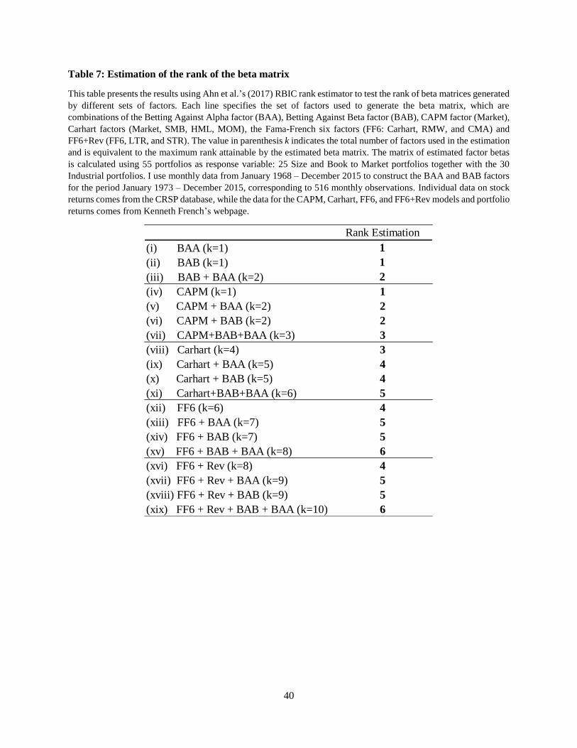
40
Table 7: Estimation of the rank of the beta matrix
This table presents the results using Ahn et al.’s (2017) RBIC rank estimator to test the rank of beta matrices generated
by different sets of factors. Each line specifies the set of factors used to generate the beta matrix, which are
combinations of the Betting Against Alpha factor (BAA), Betting Against Beta factor (BAB), CAPM factor (Market),
Carhart factors (Market, SMB, HML, MOM), the Fama-French six factors (FF6: Carhart, RMW, and CMA) and
FF6+Rev (FF6, LTR, and STR). The value in parenthesis k indicates the total number of factors used in the estimation
and is equivalent to the maximum rank attainable by the estimated beta matrix. The matrix of estimated factor betas
is calculated using 55 portfolios as response variable: 25 Size and Book to Market portfolios together with the 30
Industrial portfolios. I use monthly data from January 1968 – December 2015 to construct the BAA and BAB factors
for the period January 1973 – December 2015, corresponding to 516 monthly observations. Individual data on stock
returns comes from the CRSP database, while the data for the CAPM, Carhart, FF6, and FF6+Rev models and portfolio
returns comes from Kenneth French’s webpage.
Rank Estimation
(i) BAA (k=1) 1
(ii) BAB (k=1) 1
(iii) BAB + BAA (k=2) 2
(iv) CAPM (k=1) 1
(v) CAPM + BAA (k=2) 2
(vi) CAPM + BAB (k=2) 2
(vii) CAPM+BAB+BAA (k=3) 3
(viii) Carhart (k=4) 3
(ix) Carhart + BAA (k=5) 4
(x) Carhart + BAB (k=5) 4
(xi) Carhart+BAB+BAA (k=6) 5
(xii) FF6 (k=6) 4
(xiii) FF6 + BAA (k=7) 5
(xiv) FF6 + BAB (k=7) 5
(xv) FF6 + BAB + BAA (k=8) 6
(xvi) FF6 + Rev (k=8) 4
(xvii) FF6 + Rev + BAA (k=9) 5
(xviii) FF6 + Rev + BAB (k=9) 5
(xix) FF6 + Rev + BAB + BAA (k=10) 6
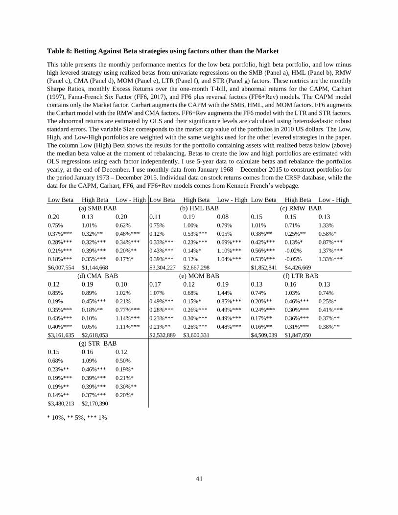
41
Table 8: Betting Against Beta strategies using factors other than the Market
This table presents the monthly performance metrics for the low beta portfolio, high beta portfolio, and low minus
high levered strategy using realized betas from univariate regressions on the SMB (Panel a), HML (Panel b), RMW
(Panel c), CMA (Panel d), MOM (Panel e), LTR (Panel f), and STR (Panel g) factors. These metrics are the monthly
Sharpe Ratios, monthly Excess Returns over the one-month T-bill, and abnormal returns for the CAPM, Carhart
(1997), Fama-French Six Factor (FF6, 2017), and FF6 plus reversal factors (FF6+Rev) models. The CAPM model
contains only the Market factor. Carhart augments the CAPM with the SMB, HML, and MOM factors. FF6 augments
the Carhart model with the RMW and CMA factors. FF6+Rev augments the FF6 model with the LTR and STR factors.
The abnormal returns are estimated by OLS and their significance levels are calculated using heteroskedastic robust
standard errors. The variable Size corresponds to the market cap value of the portfolios in 2010 US dollars. The Low,
High, and Low-High portfolios are weighted with the same weights used for the other levered strategies in the paper.
The column Low (High) Beta shows the results for the portfolio containing assets with realized betas below (above)
the median beta value at the moment of rebalancing. Betas to create the low and high portfolios are estimated with
OLS regressions using each factor independently. I use 5-year data to calculate betas and rebalance the portfolios
yearly, at the end of December. I use monthly data from January 1968 – December 2015 to construct portfolios for
the period January 1973 – December 2015. Individual data on stock returns comes from the CRSP database, while the
data for the CAPM, Carhart, FF6, and FF6+Rev models comes from Kenneth French’s webpage.
* 10%, ** 5%, *** 1%
Low Beta High Beta Low - High Low Beta High Beta Low - High Low Beta High Beta Low - High
0.20 0.13 0.20 0.11 0.19 0.08 0.15 0.15 0.13
0.75% 1.01% 0.62% 0.75% 1.00% 0.79% 1.01% 0.71% 1.33%
0.37%*** 0.32%** 0.48%*** 0.12% 0.53%*** 0.05% 0.38%** 0.25%** 0.58%*
0.28%*** 0.32%*** 0.34%*** 0.33%*** 0.23%*** 0.69%*** 0.42%*** 0.13%* 0.87%***
0.21%*** 0.39%*** 0.20%** 0.43%*** 0.14%* 1.10%*** 0.56%*** -0.02% 1.37%***
0.18%*** 0.35%*** 0.17%* 0.39%*** 0.12% 1.04%*** 0.53%*** -0.05% 1.33%***
$6,007,554 $1,144,668 $3,304,227 $2,667,298 $1,852,841 $4,426,669
0.12 0.19 0.10 0.17 0.12 0.19 0.13 0.16 0.13
0.85% 0.89% 1.02% 1.07% 0.68% 1.44% 0.74% 1.03% 0.74%
0.19% 0.45%*** 0.21% 0.49%*** 0.15%* 0.85%*** 0.20%** 0.46%*** 0.25%*
0.35%*** 0.18%** 0.77%*** 0.28%*** 0.26%*** 0.49%*** 0.24%*** 0.30%*** 0.41%***
0.43%*** 0.10% 1.14%*** 0.23%*** 0.30%*** 0.49%*** 0.17%** 0.36%*** 0.37%**
0.40%*** 0.05% 1.11%*** 0.21%** 0.26%*** 0.48%*** 0.16%** 0.31%*** 0.38%**
$3,161,635 $2,618,053 $2,532,889 $3,600,331 $4,509,039 $1,847,050
0.15 0.16 0.12
0.68% 1.09% 0.50%
0.23%** 0.46%*** 0.19%*
0.19%*** 0.39%*** 0.21%*
0.19%** 0.39%*** 0.30%**
0.14%** 0.37%*** 0.20%*
$3,480,213 $2,170,390
(g) STR BAB
(a) SMB BAB (b) HML BAB (c) RMW BAB
(d) CMA BAB (e) MOM BAB (f) LTR BAB

42
Table 9: Pricing non-Market BAB strategies using the BAA and BAB strategies as factors
This table presents the results from regressing the betting against beta strategies constructed using Smart Beta factors
(SMB, HML, RMW, CMA, MOM, LTR, and STR) on the Betting Against Alpha (BAA) and Betting Against Beta
(BAB) factors. I report pricing errors (), sensitivities to the BAA factor () and BAB factor (), and adjusted
R-squares (R2). Significance levels for the estimated parameters are calculated using heteroskedastic robust standard
errors. I use monthly data corresponding to the period January 1973 – December 2015.
* 10%, ** 5%, *** 1%
BAA BAB R2
SMB BAB 0.001 -0.01 0.70*** 0.42
HML BAB -0.002 0.97*** -0.68*** 0.54
RMW BAB 0.000 1.12*** -0.55*** 0.66
CMA BAB -0.001 1.08*** -0.82*** 0.65
MOM BAB -0.001 0.85*** 0.28** 0.74
LTR BAB -0.001 0.52*** 0.04 0.47
STR BAB -0.002 0.28*** 0.28*** 0.31

43
Table 10: Betting Against Alpha, Betting Against Beta, and Betting Against Alpha and Beta
strategies for different ranges of market capitalization
This table presents the monthly performance metrics for the low portfolio, high portfolio, and low minus high strategy
used to construct Betting Against Alpha (BAA), Betting Against Beta (BAB), and Betting Against Alpha and Beta
(BAAB) factors for sets containing assets grouped by their market capitalization value. These metrics are the monthly
Sharpe Ratios; monthly Excess Returns over the one-month T-bill; and abnormal returns for the CAPM, Carhart
(1997), Fama-French Six Factor (FF6, 2017), and FF6 plus reversal factors (FF6+Rev) models. The CAPM model
contains only the Market factor. Carhart augments the CAPM with the SMB, HML, and MOM factors. FF6 augments
the Carhart model with the RMW and CMA factors. FF6+Rev augments the FF6 model with the LTR and STR factors.
The abnormal returns are estimated by OLS and their significance levels are calculated using heteroskedastic robust
standard errors. The column Low (High) Alpha [Beta] shows the results for the portfolio containing assets with
realized alphas [betas] below (above) the median alpha [beta] value. The column Low (High) shows the results for the
portfolio containing assets with realized alphas below (above) the median alpha value within the set of assets with
realized betas below (above) the median beta value at the moment of rebalancing. Alphas and betas to create the low
and high portfolios are estimated with OLS regressions using the CAPM model. I use 5-year data to calculate alphas
and betas and rebalance the portfolios yearly, at the end of December. Additionally, at the moment of rebalancing, I
use NYSE break points to create three sets of data: (i) 30% Small, which contains all firms whose market cap is equal
to or below the 30th percentile; (ii) 40% Medium, which contains all firms whose market cap is greater than the 30th
percentile and lower than or equal to the 70th percentile; and (iii) 30% Big, which contains those firms with a market
cap value greater than the 70th percentile. I use monthly data corresponding to the period January 1968 – December
2015 to construct portfolios and factors for the period January 1973 – December 2015. Individual data on stock returns
comes from the CRSP database, while the data for the CAPM, Carhart, FF6, and FF6+Rev models comes from
Kenneth French’s webpage.
* 10%, ** 5%, *** 1%
Low High Low-High Low High Low-High Low High Low-High
30% Small 0.19 0.13 0.23 0.22 0.14 0.26 0.23 0.10 0.32
40% Medium 0.13 0.10 0.15 0.18 0.09 0.20 0.16 0.07 0.21
30% Big 0.13 0.09 0.14 0.17 0.08 0.19 0.16 0.07 0.18
30% Small 1.44% 0.80% 2.03% 0.94% 1.13% 0.85% 1.33% 0.76% 1.80%
40% Medium 0.76% 0.59% 0.96% 0.67% 0.64% 0.70% 0.75% 0.53% 0.92%
30% Big 0.64% 0.52% 0.82% 0.65% 0.51% 0.76% 0.70% 0.46% 0.91%
30% Small 0.88%*** 0.26%** 1.47%*** 0.61%*** 0.42%** 0.81%*** 0.92%*** 0.08% 1.59%***
40% Medium 0.21%* -0.02% 0.46%*** 0.32%*** -0.11% 0.64%*** 0.33%*** -0.21%* 0.75%***
30% Big 0.12%* -0.07% 0.36%** 0.28%*** -0.19%** 0.64%*** 0.29%*** -0.26%** 0.72%***
30% Small 0.82%*** 0.17%* 1.55%*** 0.44%*** 0.48%** 0.51%*** 0.73%*** 0.11% 1.31%***
40% Medium 0.13%** -0.05% 0.40%*** 0.10%* 0.00% 0.20% 0.14%** -0.08% 0.37%***
30% Big 0.08%* 0.03% 0.28%** 0.10%* 0.03% 0.20% 0.15%** -0.03% 0.34%**
30% Small 0.87%*** 0.16%* 1.76%*** 0.39%*** 0.56%*** 0.41%*** 0.69%*** 0.16% 1.28%***
40% Medium 0.08% -0.07% 0.43%*** 0.03% 0.03% 0.07% 0.06% -0.04% 0.24%*
30% Big 0.01% 0.04% 0.19% 0.00% 0.09% -0.01% 0.04% 0.10% 0.11%
30% Small 0.83%*** 0.10% 1.72%*** 0.35%*** 0.52%*** 0.35%*** 0.65%*** 0.09% 1.24%***
40% Medium 0.05% -0.09% 0.38%*** -0.02% 0.03% -0.01% 0.01% -0.05% 0.16%
30% Big -0.01% 0.02% 0.18* -0.02% 0.06% -0.04% 0.02% 0.06% 0.09%
Carhart Alpha
FF6 Alpha
FF6+Rev Alpha
Betting Against Alpha Betting Against Beta Betting Against Alpha and Beta
Sharpe Ratio
Average Returns
CAPM Alpha
44
Table 11: Betting Against Alpha, Betting Against Beta, and Betting Against Alpha and Beta factors
constructed using different holding periods for the assets
This table presents the monthly performance metrics over different holding periods for the low portfolio, high
portfolio, and low minus high strategy used to construct Betting Against Alpha (BAA), Betting Against Beta (BAB),
and Betting Against Alpha and Beta (BAAB) factors. These metrics are the monthly Sharpe Ratios; monthly Excess
Returns over the one-month T-bill; and abnormal returns for the CAPM, Carhart (1997), Fama-French Six Factor
(FF6, 2017), and FF6 plus reversal factors (FF6+Rev) models. The CAPM model contains only the Market factor.
Carhart augments the CAPM with the SMB, HML, and MOM factors. FF6 augments the Carhart model with the
RMW and CMA factors. FF6+Rev augments the FF6 model with the LTR and STR factors. The abnormal returns are
estimated by OLS and their significance levels are calculated using heteroskedastic robust standard errors. The column
Low (High) Alpha [Beta] shows the results for the portfolio containing assets with realized alphas [betas] below
(above) the median alpha [beta] value. The column Low (High) shows the results for the portfolio containing assets
with realized alphas below (above) the median alpha value within the set of assets with realized betas below (above)
the median beta value at the moment of rebalancing. Alphas and betas to create the low and high portfolios are
estimated with OLS regressions using the CAPM model. I use 5-year data to calculate alphas and betas and rebalance
the portfolios using the following frequencies: 1, 6, 12, 24, and 48 months. I use monthly data corresponding to the
period January 1968 – December 2015 to construct portfolios and low-high strategies for the period January 1973 –
December 2015. Individual data on stock returns comes from the CRSP database, while the data for the CAPM,
Carhart, FF6, and FF6+Rev models comes from Kenneth French’s webpage.

45
* 10%, ** 5%, *** 1%
Low AlphaHigh AlphaLow-High Low Beta High Beta Low-High Low High Low-High
1 month 0.17 0.13 0.18 0.22 0.11 0.28 0.21 0.10 0.25
6 month 0.16 0.13 0.18 0.22 0.12 0.27 0.21 0.10 0.26
12 month 0.18 0.12 0.22 0.22 0.12 0.26 0.22 0.09 0.30
24 month 0.20 0.12 0.24 0.22 0.13 0.24 0.24 0.09 0.35
48 month 0.21 0.13 0.25 0.22 0.14 0.23 0.24 0.10 0.34
1 month 1.10% 0.77% 1.45% 0.82% 0.87% 0.87% 1.05% 0.70% 1.38%
6 month 1.07% 0.75% 1.39% 0.81% 0.89% 0.80% 1.02% 0.75% 1.30%
12 month 1.15% 0.67% 1.60% 0.81% 0.90% 0.79% 1.08% 0.61% 1.47%
24 month 1.25% 0.64% 1.75% 0.82% 0.96% 0.70% 1.18% 0.59% 1.65%
48 month 1.23% 0.72% 1.53% 0.81% 1.01% 0.66% 1.05% 0.68% 1.25%
1 month 0.55%*** 0.19%** 0.92%*** 0.49%*** 0.14% 0.82%*** 0.65%*** -0.01% 1.19%***
6 month 0.52%*** 0.17%* 0.88%*** 0.48%*** 0.16% 0.75%*** 0.63%*** -0.01% 1.13%***
12 month 0.60%*** 0.10% 1.10%*** 0.47%*** 0.18% 0.73%*** 0.68%*** -0.10% 1.29%***
24 month 0.69%*** 0.08% 1.22%*** 0.47%*** 0.25%*** 0.65%*** 0.76%*** -0.09% 1.44%***
48 month 0.69%*** 0.14%* 1.06%*** 0.46%*** 0.31%** 0.57%*** 0.66%*** 0.00% 1.09%***
1 month 0.55%*** 0.12%** 1.08%*** 0.31%*** 0.25%*** 0.45%*** 0.53%*** 0.04% 1.00%***
6 month 0.49%*** 0.12%** 0.95%*** 0.30%*** 0.26%*** 0.40%*** 0.49%*** 0.07% 0.88%***
12 month 0.55%*** 0.06% 1.12%*** 0.30%*** 0.27%*** 0.40%*** 0.52%*** 0.00% 1.00%***
24 month 0.61%*** 0.07% 1.16%*** 0.29%*** 0.33%*** 0.31%*** 0.58%*** 0.02% 1.10%***
48 month 0.60%*** 0.12%** 1.04%*** 0.29%*** 0.37%*** 0.26%** 0.51%*** 0.08% 0.83%***
1 month 0.56%*** 0.14%** 1.18%*** 0.26%*** 0.33%*** 0.35%*** 0.48%*** 0.12%* 0.91%***
6 month 0.49%*** 0.12%* 1.06%*** 0.24%*** 0.32%*** 0.29%*** 0.44%*** 0.13%* 0.81%***
12 month 0.55%*** 0.05% 1.24%*** 0.24%*** 0.32%*** 0.29%*** 0.47%*** 0.04% 0.94%***
24 month 0.62%*** 0.02% 1.34%*** 0.23%*** 0.36%*** 0.21%** 0.53%*** 0.01% 1.09%***
48 month 0.56%*** 0.10%** 1.11%*** 0.25%*** 0.39%*** 0.22%** 0.42%*** 0.10%** 0.80%***
1 month 0.49%*** 0.12%** 1.08%*** 0.23%*** 0.28%*** 0.33%*** 0.43%*** 0.10% 0.82%***
6 month 0.45%*** 0.09% 1.00%*** 0.21%*** 0.29%*** 0.24%** 0.39%*** 0.09% 0.75%***
12 month 0.52%*** 0.01% 1.20%*** 0.20%*** 0.29%*** 0.23%** 0.43%*** -0.01% 0.89%***
24 month 0.59%*** -0.02% 1.31%*** 0.19%*** 0.34%*** 0.15% 0.50%*** -0.04% 1.05%***
48 month 0.53%*** 0.07% 1.07%*** 0.21%*** 0.37%*** 0.15% 0.39%*** 0.07% 0.76%***
CAPM Alpha
Carhart Alpha
FF6 Alpha
FF6+Rev Alpha
Betting Against Alpha Betting Against Beta Betting Against Alpha and Beta
Sharpe Ratio
Average Returns
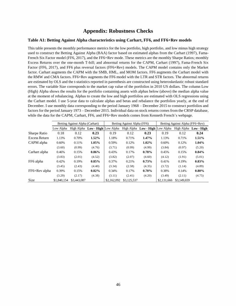
46
Appendix: Robustness Checks
Table A1: Betting Against Alpha characteristics using Carhart, FF6, and FF6+Rev models
This table presents the monthly performance metrics for the low portfolio, high portfolio, and low minus high strategy
used to construct the Betting Against Alpha (BAA) factor based on estimated alphas from the Carhart (1997), Fama-
French Six Factor model (FF6, 2017), and the FF6+Rev mode. These metrics are the monthly Sharpe Ratios; monthly
Excess Returns over the one-month T-bill; and abnormal returns for the CAPM, Carhart (1997), Fama-French Six
Factor (FF6, 2017), and FF6 plus reversal factors (FF6+Rev) models. The CAPM model contains only the Market
factor. Carhart augments the CAPM with the SMB, HML, and MOM factors. FF6 augments the Carhart model with
the RMW and CMA factors. FF6+Rev augments the FF6 model with the LTR and STR factors. The abnormal returns
are estimated by OLS and the t-statistics reported in parenthesis are constructed using heteroskedastic robust standard
errors. The variable Size corresponds to the market cap value of the portfolios in 2010 US dollars. The column Low
(High) Alpha shows the results for the portfolio containing assets with alphas below (above) the median alpha value
at the moment of rebalancing. Alphas to create the low and high portfolios are estimated with OLS regressions using
the Carhart model. I use 5-year data to calculate alphas and betas and rebalance the portfolios yearly, at the end of
December. I use monthly data corresponding to the period January 1968 – December 2015 to construct portfolios and
factors for the period January 1973 – December 2015. Individual data on stock returns comes from the CRSP database,
while the data for the CAPM, Carhart, FF6, and FF6+Rev models comes from Kenneth French’s webpage.
Low Alpha High Alpha Low - High Low Alpha High Alpha Low - High Low Alpha High Alpha Low - High
Sharpe Ratio 0.18 0.12 0.23 0.19 0.12 0.23 0.19 0.12 0.24
Excess Return 1.13% 0.70% 1.52% 1.18% 0.71% 1.47% 1.13% 0.71% 1.51%
CAPM alpha 0.60% 0.11% 1.05% 0.59% 0.12% 1.02% 0.60% 0.12% 1.04%
(3.60) (0.99) (4.76) (3.71) (0.99) (4.99) (3.84) (0.97) (5.20)
Carhart alpha 0.46% 0.15% 0.86% 0.43% 0.17% 0.78% 0.45% 0.15% 0.84%
(3.83) (2.01) (4.52) (3.82) (2.07) (4.60) (4.12) (1.91) (5.01)
FF6 alpha 0.42% 0.19% 0.85% 0.37% 0.21% 0.73% 0.41% 0.19% 0.83%
(3.45) (2.43) (4.40) (3.34) (2.58) (4.35) (3.72) (1.14) (4.89)
FF6+Rev alpha 0.39% 0.15% 0.82% 0.34% 0.17% 0.70% 0.38% 0.14% 0.80%
(3.29) (2.17) (4.38) (3.11) (2.41) (4.20) (3.49) (2.11) (4.75)
Size $1,840,154 $3,443,087 $2,162,092 $3,125,537 $2,131,666 $3,149,659
Betting Against Alpha (Carhart) Betting Against Alpha (FF6) Betting Against Alpha (FF6+Rev)
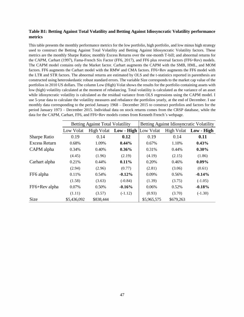
47
Table B1: Betting Against Total Volatility and Betting Against Idiosyncratic Volatility performance
metrics
This table presents the monthly performance metrics for the low portfolio, high portfolio, and low minus high strategy
used to construct the Betting Against Total Volatility and Betting Against Idiosyncratic Volatility factors. These
metrics are the monthly Sharpe Ratios; monthly Excess Returns over the one-month T-bill; and abnormal returns for
the CAPM, Carhart (1997), Fama-French Six Factor (FF6, 2017), and FF6 plus reversal factors (FF6+Rev) models.
The CAPM model contains only the Market factor. Carhart augments the CAPM with the SMB, HML, and MOM
factors. FF6 augments the Carhart model with the RMW and CMA factors. FF6+Rev augments the FF6 model with
the LTR and STR factors. The abnormal returns are estimated by OLS and the t-statistics reported in parenthesis are
constructed using heteroskedastic robust standard errors. The variable Size corresponds to the market cap value of the
portfolios in 2010 US dollars. The column Low (High) Volat shows the results for the portfolio containing assets with
low (high) volatility calculated at the moment of rebalancing. Total volatility is calculated as the variance of an asset
while idiosyncratic volatility is calculated as the residual variance from OLS regressions using the CAPM model. I
use 5-year data to calculate the volatility measures and rebalance the portfolios yearly, at the end of December. I use
monthly data corresponding to the period January 1968 – December 2015 to construct portfolios and factors for the
period January 1973 – December 2015. Individual data on stock returns comes from the CRSP database, while the
data for the CAPM, Carhart, FF6, and FF6+Rev models comes from Kenneth French’s webpage.
Low Volat High Volat Low - High Low Volat High Volat Low - High
Sharpe Ratio 0.19 0.14 0.12 0.19 0.14 0.11
Excess Return 0.68% 1.09% 0.44% 0.67% 1.10% 0.43%
CAPM alpha 0.34% 0.40% 0.36% 0.31% 0.44% 0.30%
(4.45) (1.96) (2.19) (4.19) (2.15) (1.86)
Carhart alpha 0.21% 0.44% 0.11% 0.20% 0.46% 0.09%
(2.94) (2.96) (0.77) (2.81) (3.06) (0.61)
FF6 alpha 0.11% 0.54% -0.12% 0.09% 0.56% -0.14%
(1.58) (3.63) (-0.84) (1.39) (3.75) (-1.05)
FF6+Rev alpha 0.07% 0.50% -0.16% 0.06% 0.52% -0.18%
(1.11) (3.57) (-1.12) (0.93) (3.70) (-1.30)
Size $5,436,092 $838,444 $5,965,575 $679,263
Betting Against Total Volatility Betting Against Idiosyncratic Volatility
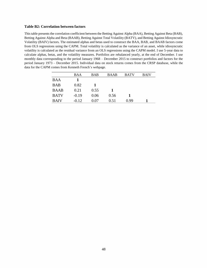
48
Table B2: Correlation between factors
This table presents the correlation coefficient between the Betting Against Alpha (BAA), Betting Against Beta (BAB),
Betting Against Alpha and Beta (BAAB), Betting Against Total Volatility (BATV), and Betting Against Idiosyncratic
Volatility (BAIV) factors. The estimated alphas and betas used to construct the BAA, BAB, and BAAB factors come
from OLS regressions using the CAPM. Total volatility is calculated as the variance of an asset, while idiosyncratic
volatility is calculated as the residual variance from an OLS regressions using the CAPM model. I use 5-year data to
calculate alphas, betas, and the volatility measures. Portfolios are rebalanced yearly, at the end of December. I use
monthly data corresponding to the period January 1968 – December 2015 to construct portfolios and factors for the
period January 1973 – December 2015. Individual data on stock returns comes from the CRSP database, while the
data for the CAPM comes from Kenneth French’s webpage.
BAA BAB BAAB BATV BAIV
BAA 1
BAB 0.82 1
BAAB 0.21 0.55 1
BATV -0.19 0.06 0.56 1
BAIV -0.12 0.07 0.51 0.99 1