BET’s

BASAVAKALYAN ENGINEERING COLLEGE

BASAVAKALYAN

Department

Of

Computer Science & Engineering

COMPUTER NETWORK Laboratory

(15cs l57)

V Semester (CBCS)

Prepared by:-

Mr. Gangadhar G H Asst. Professor

Mrs. Sangeeta K Instructor

COMPUTER NETWORK LABORATORY [As per Choice Based Credit System (CBCS) scheme]

(Effective from the academic year 2016 -2017)

SEMESTER – V

Subject Code: 15CSL57 IA Marks: 20

Number of Lecture Hours/Week: 01I + 02P Exam

Marks: 80

Total Number of Lecture Hours: 40 Exam Hours:

03

CREDITS – 02

Course objectives: This course will enable students to

Demonstrate operation of network and its management commands

Simulate and demonstrate the performance of GSM and CDMA

Implement data link layer and transport layer protocols.

Description (If any):

For the experiments below modify the topology and parameters set for the experiment and

take multiple rounds of reading and analyze the results available in log files. Plot necessary

graphs and conclude using any suitable tool.

Lab Experiments:

PART A

1. Implement three nodes point – to – point network with duplex links between them. Set the

queue size, vary the bandwidth and find the number of packets dropped.

2. Implement transmission of ping messages/trace route over a network topology consisting of

6 nodes and find the number of packets dropped due to congestion.

3. Implement an Ethernet LAN using n nodes and set multiple traffic nodes and plot

congestion

window for different source / destination.

4. Implement simple ESS and with transmitting nodes in wire-less LAN by simulation and

determine the performance with respect to transmission of packets.

5. Implement and study the performance of GSM on NS2/NS3 (Using MAC layer) or

equivalent environment.

6. Implement and study the performance of CDMA on NS2/NS3 (Using stack called Call net)

or equivalent environment.

PART B

Implement the following in Java:

7. Write a program for error detecting code using CRC-CCITT (16- bits).

8. Write a program to find the shortest path between vertices using bellman-ford algorithm.

9. Using TCP/IP sockets, write a client – server program to make the client send the file name

and to make the server send back the contents of the requested file if present. Implement the

above program using as message queues or FIFOs as IPC channels.

10. Write a program on datagram socket for client/server to display the messages on client side,

typed at the server side.

11. Write a program for simple RSA algorithm to encrypt and decrypt the data.

12. Write a program for congestion control using leaky bucket algorithm.

Study Experiment / Project:

NIL

Course outcomes: The students should be able to:

Analyze and Compare various networking protocols.

Demonstrate the working of different concepts of networking.

Implement, analyze and evaluate networking protocols in NS2 / NS3

Conduction of Practical Examination:

1. All laboratory experiments are to be included for practical examination.

2. Students are allowed to pick one experiment from part A and part B with lot.

3. Strictly follow the instructions as printed on the cover page of answer script

4. Marks distribution: Procedure + Conduction + Viva: 80

Part A: 5+30+5 =40

Part B: 5+30+5 =40

5. Change of experiment is allowed only once and marks allotted to the procedure part to be

made zero.

Part A - SIMULATION USING NS-2

Introduction to NS-2: NS2 is an open-source simulation tool that runs on Linux. It is a discreet event

simulator targeted at networking research and provides substantial support for simulation of

routing, multicast protocols and IP protocols, such as UDP, TCP, RTP and SRM over wired and wireless (local and satellite) networks.

Widely known as NS2, is simply an event driven simulation tool.

Useful in studying the dynamic nature of communication networks.

Simulation of wired as well as wireless network functions and protocols

(e.g., routing algorithms, TCP, UDP) can be done using NS2.

In general, NS2 provides users with a way of specifying such network protocols

and simulating their corresponding behaviors.

Basic Architecture of NS2

TCL – Tool Command Language

Tcl is a very simple programming language. If you have programmed before, you

can learn enough to write interesting Tcl programs within a few hours. This page provides a quick overview of the main features of Tcl. After reading this you'll probably be able to

start writing simple Tcl scripts on your own; however, we recommend that you consult one

of the many available Tcl books for more complete information.

Basic syntax

Tcl scripts are made up of commands separated by newlines or semicolons.

Commands all have the same basic form illustrated by the following example:

expr 20 + 10

This command computes the sum of 20 and 10 and returns the result, 30. You can try out this example and all the others in this page by typing them to a Tcl application such as tclsh; after a command completes, tclsh prints its result.

Each Tcl command consists of one or more words separated by spaces. In this example there are four words: expr, 20, +, and 10. The first word is the name of a command and the other words are arguments to that command. All Tcl commands consist of words,

but different commands treat their arguments differently. The expr command treats all of its arguments together as an arithmetic expression, computes the result of that expression, and

returns the result as a string. In the expr command the division into words isn't significant: you could just as easily have invoked the same command as

expr 20+10

However, for most commands the word structure is important, with each word used for a distinct purpose.

All Tcl commands return results. If a command has no meaningful result then it returns an empty string as its result.

Variables

Tcl allows you to store values in variables and use the values later in commands.

The set command is used to write and read variables. For example, the following command modifies the variable x to hold the value 32:

set x 32

The command returns the new value of the variable. You can read the value of a variable by invoking set with only a single argument:

set x

You don't need to declare variables in Tcl: a variable is created automatically the

first time it is set. Tcl variables don't have types: any variable can hold any value.

To use the value of a variable in a command, use variable substitution as in the following example:

expr $x*3

When a $ appears in a command, Tcl treats the letters and digits following it as a

variable name, and substitutes the value of the variable in place of the name. In this

example, the actual argument received by the expr command will be 32*3 (assuming that variable x was set as in the previous example). You can use variable substitution in any

word of any command, or even multiple times within a word:

set cmd expr

set x 11

$cmd $x*$x

Command substitution

You can also use the result of one command in an argument to another command. This is called command substitution:

set a 44

set b [expr $a*4]

When a [ appears in a command, Tcl treats everything between it and the matching ]

as a nested Tcl command. Tcl evaluates the nested command and substitutes its result into the enclosing command in place of the bracketed text. In the example above the second

argument of the second set command will be 176.

Quotes and braces

Double-quotes allow you to specify words that contain spaces. For example, consider the following script:

set x 24

set y 18

set z "$x + $y is [expr $x + $y]"

After these three commands are evaluated variable z will have the value 24 + 18 is 42. Everything between the quotes is passed to the set command as a single word. Note that (a)

command and variable substitutions are performed on the text between the quotes, and (b) the quotes themselves are not passed to the command. If the quotes were not present, the set

command would have received 6 arguments, which would have caused an error.

Curly braces provide another way of grouping information into words. They are different from quotes in that no substitutions are performed on the text between the curly braces:

set z {$x + $y is [expr $x + $y]}

This command sets variable z to the value "$x + $y is [expr $x + $y]".

Control structures

Tcl provides a complete set of control structures including commands for conditional execution, looping, and procedures. Tcl control structures are just commands

that take Tcl scripts as arguments. The example below creates a Tcl procedure called power, which raises a base to an integer power:

proc power {base p} {

set result 1

while {$p > 0} {

set result [expr $result * $base]

set p [expr $p - 1]

} return $result

}

This script consists of a single command, proc. The proc command takes three

arguments: the name of a procedure, a list of argument names, and the body of the

procedure, which is a Tcl script. Note that everything between the curly brace at the end of

the first line and the curly brace on the last line is passed verbatim to proc as a single

argument. The proc command creates a new Tcl command named power that takes two

arguments. You can then invoke power with commands like the following:

power 2 6

power 1.15 5

When power is invoked, the procedure body is evaluated. While the body is executing it can access its arguments as variables: base will hold the first argument and p will hold the second.

The body of the power procedure contains three Tcl commands: set, while, and return.

The while command does most of the work of the procedure. It takes two arguments, an

expression ($p > 0) and a body, which is another Tcl script. The while command evaluates its

expression argument using rules similar to those of the C programming language and if the

result is true (nonzero) then it evaluates the body as a Tcl script. It repeats this process over

and over until eventually the expression evaluates to false (zero). In this case the body of

the while command multiplied the result value by base and then decrements p. When p

reaches zero the result contains the desired power of base. The return command causes the

procedure to exit with the value of variable result as the procedure's result.

Where do commands come from?

As you have seen, all of the interesting features in Tcl are represented by commands. Statements are commands, expressions are evaluated by executing commands, control structures are commands, and procedures are commands.

Tcl commands are created in three ways. One group of commands is provided by

the Tcl interpreter itself. These commands are called builtin commands. They include all of the commands you have seen so far and many more (see below). The builtin commands are

present in all Tcl applications.

The second group of commands is created using the Tcl extension mechanism. Tcl

provides APIs that allow you to create a new command by writing a command procedure in

C or C++ that implements the command. You then register the command procedure with

the Tcl interpreter by telling Tcl the name of the command that the procedure implements.

In the future, whenever that particular name is used for a Tcl command, Tcl will call your

command procedure to execute the command. The builtin commands are also implemented

using this same extension mechanism; their command procedures are simply part of the Tcl

library.

When Tcl is used inside an application, the application incorporates its key features

into Tcl using the extension mechanism. Thus the set of available Tcl commands varies

from application to application. There are also numerous extension packages that can be

incorporated into any Tcl application. One of the best known extensions is Tk, which

provides powerful facilities for building graphical user interfaces. Other extensions provide

object-oriented programming, database access, more graphical capabilities, and a variety of

other features. One of Tcl's greatest advantages for building integration applications is the

ease with which it can be extended to incorporate new features or communicate with other

resources.

The third group of commands consists of procedures created with the proc command, such as the power command created above. Typically, extensions are used for

lower-level functions where C programming is convenient, and procedures are used for higher-level functions where it is easier to write in Tcl.

Wired TCL Script Components

Create the event scheduler

Open new files & turn on the tracing

Create the nodes

Setup the links

Configure the traffic type (e.g., TCP, UDP, etc)

Set the time of traffic generation (e.g., CBR, FTP)

Terminate the simulation

NS Simulator Preliminaries.

Initialization and termination aspects of the ns simulator.

Definition of network nodes, links, queues and topology.

Definition of agents and of applications.

The nam visualization tool.

Tracing and random variables.

Features of NS2

NS2 can be employed in most unix systems and windows. Most of the NS2 code is in C++. It uses TCL as its scripting language, Otcl adds object orientation to

TCL.NS(version 2) is an object oriented, discrete event driven network simulator that is freely distributed and open source.

• Traffic Models: CBR, VBR, Web etc

• Protocols: TCP, UDP, HTTP, Routing algorithms,MAC etc

• Error Models: Uniform, bursty etc

• Misc: Radio propagation, Mobility models , Energy Models

• Topology Generation tools

• Visualization tools (NAM), Tracing

Structure of NS

● NS is an object oriented discrete event simulator

– Simulator maintains list of events and executes one event after another

– Single thread of control: no locking or race conditions

● Back end is C++ event scheduler

– Protocols mostly

– Fast to run, more control

• Front end is OTCL

Creating scenarios, extensions to C++ protocols

fast to write and change

Platforms

It can be employed in most unix systems(FreeBSD, Linux, Solaris) and Windows.

Source code

Most of NS2 code is in C++

Scripting language

It uses TCL as its scripting language OTcl adds object orientation to TCL.

Protocols implemented in NS2

Transport layer(Traffic Agent) – TCP, UDP

Network layer(Routing agent)

Interface queue – FIFO queue, Drop Tail queue, Priority queue

Logic link contol layer – IEEE 802.2, AR

How to use NS2

Design Simulation – Determine simulation scenario

Build ns-2 script using tcl.

Run simulation

Simulation with NS2

Define objects of simulation.

Connect the objects to each other

Start the source applications. Packets are then created and are transmitted through network.

Exit the simulator after a certain fixed time.

NS programming Structure

● Create the event scheduler

● Turn on tracing

● Create network topology

● Create transport connections

● Generate traffic

● Insert errors

Sample Wired Simulation using NS-2

Creating Event Scheduler

● Create event scheduler: set ns [new simulator]

● Schedule an event: $ns at <time> <event>

– event is any legitimate ns/tcl function

$ns at 5.0 “finish”

proc finish {} {

global ns nf

close $nf

exec nam out.nam &

exit 0

}

● Start Scheduler

$ns run

Tracing

● All packet trace

$ns traceall[open out.tr w]

<event> <time> <from> <to> <pkt> <size>

…

<flowid> <src> <dst> <seqno> <aseqno>

+ 0.51 0 1 cbr 500 —– 0 0.0 1.0 0 2

_ 0.51 0 1 cbr 500 —– 0 0.0 1.0 0 2

R 0.514 0 1 cbr 500 —–0 0.0 1.0 0 0

● Variable trace

set par [open output/param.tr w]

$tcp attach $par

$tcp trace cwnd_

$tcp trace maxseq_

$tcp trace rtt_

Tracing and Animation

● Network Animator

set nf [open out.nam w]

$ns namtraceall

$nf

proc finish {} {

global ns nf

close $nf

exec nam out.nam &

exit 0

}

Creating topology

● Two nodes connected by a link

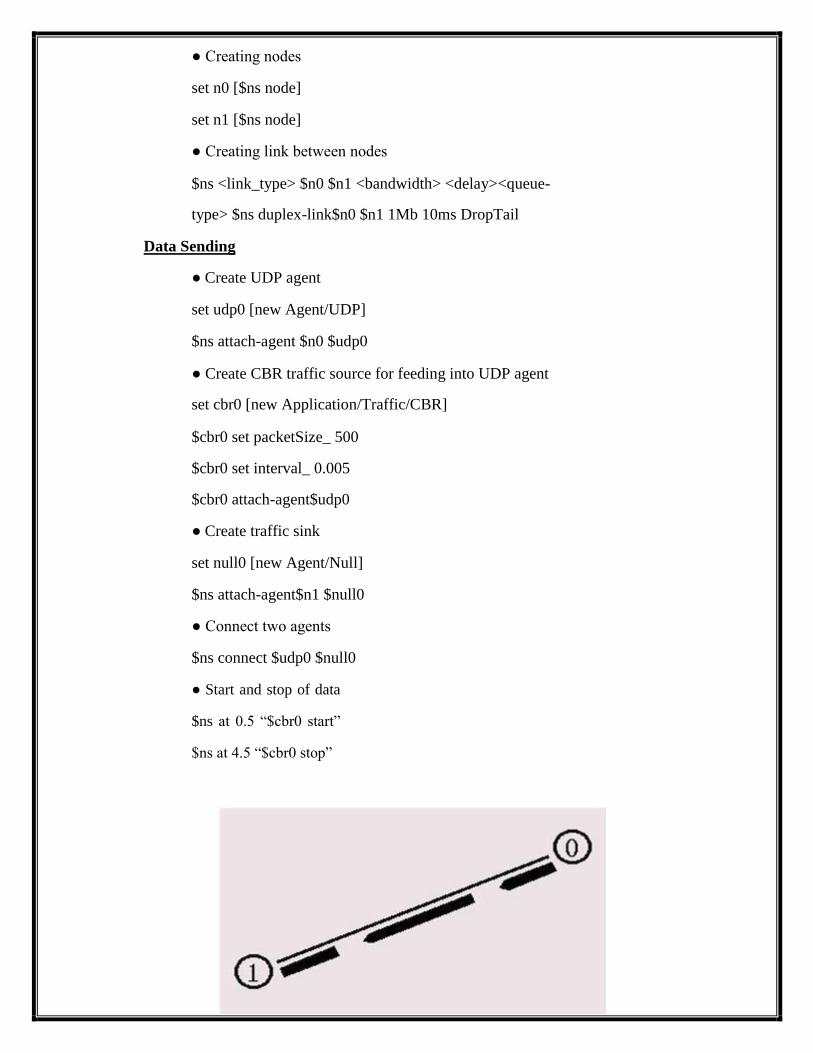
● Creating nodes

set n0 [$ns node]

set n1 [$ns node]

● Creating link between nodes

$ns <link_type> $n0 $n1 <bandwidth> <delay><queue-

type> $ns duplex-link$n0 $n1 1Mb 10ms DropTail

Data Sending

● Create UDP agent

set udp0 [new Agent/UDP]

$ns attach-agent $n0 $udp0

● Create CBR traffic source for feeding into UDP agent

set cbr0 [new Application/Traffic/CBR]

$cbr0 set packetSize_ 500

$cbr0 set interval_ 0.005

$cbr0 attach-agent$udp0

● Create traffic sink

set null0 [new Agent/Null]

$ns attach-agent$n1 $null0

● Connect two agents

$ns connect $udp0 $null0

● Start and stop of data

$ns at 0.5 “$cbr0 start”

$ns at 4.5 “$cbr0 stop”

Traffic on top of TCP

● FTP

set ftp [new Application/FTP]

$ftp attach-agent$tcp0

● Telnet

set telnet [new Application/Telnet]

$telnet attach-agent$tcp0

PROCEDURE

STEP 1: Start

STEP 2: Create the simulator object ns for designing the given simulation

STEP 3: Open the trace file and nam file in the write mode

STEP 4: Create the nodes of the simulation using the ‘set’ command

STEP 5: Create links to the appropriate nodes using $ns duplex-link command

STEP 6: Set the orientation for the nodes in the simulation using ‘orient’ command

STEP 7: Create TCP agent for the nodes and attach these agents to the nodes

STEP 8: The traffic generator used is FTP for both node0 and node1

STEP 9: Configure node1 as the sink and attach it

STEP10: Connect node0 and node1 using ‘connect’ command

STEP 11: Setting color for the nodes

STEP 12: Schedule the events for FTP agent 10 sec

STEP 13: Schedule the simulation for 5 minutes

Structure of Trace Files

When tracing into an output ASCII file, the trace is organized in 12 fields as follows in fig shown below,

The meaning of the fields are:

Event Time From To PKT PKT Flags Fid Src Dest Seq Pkt

Node Node Type Size Addr Addr Num id

1. The first field is the event type. It is given by one of four possible symbols r, +, -, d

which correspond respectively to receive (at the output of the link), enqueued,

dequeued and dropped.

2. The second field gives the time at which the event occurs.

3. Gives the input node of the link at which the event occurs.

4. Gives the output node of the link at which the event occurs.

5. Gives the packet type (eg CBR or TCP)

6. Gives the packet size

7. Some flags

8. This is the flow id (fid) of IPv6 that a user can set for each flow at the input

OTcl script one can further use this field for analysis purposes; it is also used

when specifying stream color for the NAM display.

9. This is the source address given in the form of ―node.port‖.

10. This is the destination address, given in the same form.

11. This is the network layer protocol’s packet sequence number. Even though UDP

implementations in a real network do not use sequence number, ns keeps track of

UDP packet sequence number for analysis purposes

12. The last field shows the Unique id of the packet.

XGRAPH

The xgraph program draws a graph on an x-display given data read from either data

file or from standard input if no files are specified. It can display upto 64 independent data

sets using different colors and line styles for each set. It annotates the graph with a title,

axis labels, grid lines or tick marks, grid labels and a legend.

Syntax: Xgraph [options] file-name

Options are listed here

/-bd <color> (Border)

This specifies the border color of the xgraph window.

/-bg <color> (Background)

This specifies the background color of the xgraph window.

/-fg<color> (Foreground)

This specifies the foreground color of the xgraph window.

/-lf <fontname> (LabelFont)

All axis labels and grid labels are drawn using this font.

/-t<string> (Title Text)

This string is centered at the top of the graph.

/-x <unit name> (XunitText)

This is the unit name for the x-axis. Its default is ―X‖.

/-y <unit name> (YunitText)

This is the unit name for the y-axis. Its default is ―Y‖.

INTRODUCTION

Network simulation is an important tool in developing, testing and evaluating network

protocols. Simulation can be used without the target physical hardware, making it economical and practical for almost any scale of network topology and setup. It is possible to simulate a link of any bandwidth and delay, even if such a link is currently impossible in the real world. With simulation, it is possible to set each simulated node to use any desired software. This means that meaning deploying software is not an issue. Results are also easier to obtain and analyze, because extracting information from important points in the simulated network is as done by simply parsing the generated trace files.

Simulation is only of use if the results are accurate, an inaccurate simulator is not useful at

all. Most network simulators use abstractions of network protocols, rather than the real thing, making their results less convincing. S.Y. Wang reports that the simulator OPNET uses a simplified finite state machine to model complex TCP protocol processing. [19] NS-2 uses a model based on BSD TCP, it is implemented as a set of classes using inheritance. Neither uses protocol code that is used in real world networking.

Improving Network Simulation:

Wang states that “Simulation results are not as convincing as those produced by real

hardware and software equipment.” This statement is followed by an explanation of the fact that most existing network simulators can only simulate real life network protocol implementations with limited detail, which can lead to incorrect results. Another paper includes a similar statement, “running the actual TCP code is preferred to running an

abstract specification of the protocol.” Brakmo and Peterson go on to discuss how the BSD implementations of TCP are quite important with respect to timers. Simulators often use more accurate round trip time measurements than those used in the BSD implementation, making results differ.

Using real world network stacks in a simulator should make results more accurate, but it is not clear how such stacks should be integrated with a simulator. The network simulator NCTUns shows how it is possible to use the network stack of the simulators machine.

Network Simulation Experience

The Network Simulator offers a simplified and complete network simulation experience.

The following diagram depicts this functionality offered by the Network Simulator.

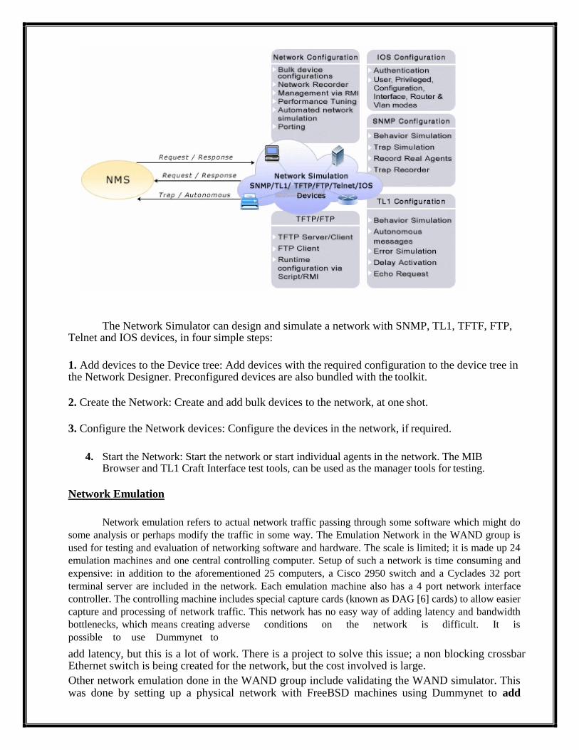
The Network Simulator can design and simulate a network with SNMP, TL1, TFTF, FTP, Telnet and IOS devices, in four simple steps:

1. Add devices to the Device tree: Add devices with the required configuration to the device tree in the Network Designer. Preconfigured devices are also bundled with the toolkit.

2. Create the Network: Create and add bulk devices to the network, at one shot.

3. Configure the Network devices: Configure the devices in the network, if required.

4. Start the Network: Start the network or start individual agents in the network. The MIB

Browser and TL1 Craft Interface test tools, can be used as the manager tools for testing.

Network Emulation

Network emulation refers to actual network traffic passing through some software which might do

some analysis or perhaps modify the traffic in some way. The Emulation Network in the WAND group is

used for testing and evaluation of networking software and hardware. The scale is limited; it is made up 24

emulation machines and one central controlling computer. Setup of such a network is time consuming and

expensive: in addition to the aforementioned 25 computers, a Cisco 2950 switch and a Cyclades 32 port

terminal server are included in the network. Each emulation machine also has a 4 port network interface

controller. The controlling machine includes special capture cards (known as DAG [6] cards) to allow easier

capture and processing of network traffic. This network has no easy way of adding latency and bandwidth

bottlenecks, which means creating adverse conditions on the network is difficult. It is

possible to use Dummynet to

add latency, but this is a lot of work. There is a project to solve this issue; a non blocking crossbar Ethernet switch is being created for the network, but the cost involved is large.

Other network emulation done in the WAND group include validating the WAND simulator. This was done by setting up a physical network with FreeBSD machines using Dummynet to add

latency. Dummynet is one example of network emulation software, NIST Net is another, it claims to “allow controlled, reproducible experiments with network performance sensitive/adaptive applications and control protocols in a simple laboratory setting”.

NS-2 also provides some network emulation functionality, it is able to capture packets from

the live network and drop, delay, re-order, or duplicate them. Emulation, especially in the case of a network simulator like NS-2, is interesting because it is using real world data from real world network stacks. Emulation offers something simulation never can: it is performed on a real network, using actual equipment and real software. However, it is very limited compared to simulation in other areas; for example scale. The WAND Emulation Network described earlier requires a lot of setup and is expensive, yet only contains 24 emulation machines. There is no theoretical limit to the number of nodes a simulator can handle, and increasing the size of a simulation does not cost anything. The factors to consider are RAM, disk space and the small amount of time taken to change a simulation script. In general, changing the simulation is a simple step, though it would be complex in the case a huge amount of nodes being required (a million, for example).

Also, network emulation must of course be run in real time, where simulation can

sometimes simulate large time periods in a small amount of time. In the case of a million nodes, the simulation might run in greater than real time because the hardware it is run on would limit performance.

Introduction to Network Simulators

Network simulators implemented in software are valuable tools for researchers to develop,

test, and diagnose network protocols. Simulation is economical because it can carry out experiments without the actual hardware. It is flexible because it can, for example, simulate a link with any bandwidth and propagation delay. Simulation results are easier to analyze than experimental results because important information at critical points can be easily logged to help researchers diagnose network protocols.

Network simulators, however, have their limitations. A complete network simulator needs

to simulate networking devices (e.g., hosts and routers) and application programs that generate network traffic. It also needs to provide network utility programs to configure, monitor, and gather statistics about a simulated network. Therefore, developing a complete network simulator is a large effort. Due to limited development resources, traditional network simulators usually have the following drawbacks:

• Simulation results are not as convincing as those produced by real hardware and software equipment. In order to constrain their complexity and development cost, most network simulators usually can only simulate real-life network protocol implementations with limited details, and this may lead to incorrect results.

• These simulators are not extensible in the sense that they lack the standard UNIX POSIX application programming interface (API). As such, existing or to-be-developed real-life application programs cannot run normally to generate traffic for a simulated network. Instead, they must be rewritten to use the internal API provided by the simulator (if there is any) and be compiled with the simulator to form a single, big, and complex program.

To overcome these problems, Wang invented a kernel re-entering simulation methodology and

used it to implement the Harvard network simulator. Later on, Wang further improved the methodology and

used it to design and implement the NCTUns network simulator and emulator.

Different types of simulators

Some of the different types of simulators are as follows:-

s MIT's NETSIM s NIST s CPSIM s INSANE s NEST s REAL s NS s OPNET

s NCTUns

A brief explanation of some of the above simulators is as follows:-

REAL

REAL (REalistic And Large) is a network simulator written at Cornell University by

S. Keshav and based on a modified version of NEST 2.5.

Use NEST is intended for studying the dynamic behavior of flow and congestion control

schemes in packet-switched data networks (namely TCP/IP).

The package REAL provides 30 modules written in C that emulate flow-control protocols such as TCP,

and 5 scheduling disciplines such as FIFO, Fair Queuing, DEC congestion avoidance and Hierarchical Round Robin.

The description of the network topology, protocols workload and control parameters are transmitted to the server using a simple ASCII representation called NetLanguage where the network is modeled as a graph. This latest release now includes a GUI written in Java.

Implementation of the simulator

The NEST code has been rewritten to make it less general, cleaner and faster. REAL is still

implemented as a client-server program. The code is freely available to anyone willing to modify it.

Node functions implement computation at each node in the network whereas queue management and

routing functions manage buffers in nodes and packet switching. Routing is static and is based on

Dijkstras's shortest path algorithm. A node could be a source, a router or a sink. Source nodes

implement TCP-like transport layer functionality. Routers implement the scheduling disciplines, while

the sinks are universal receivers that only acknowledge packets.

Since NEST didn't not allow for timers, REAL sends out a timer packet from a source back

to itself to return after some specified time, but timers cannot be reset using this method.

NCTUns

Introduction

NCTUns is open source, high quality, and supports many types of networks.The NCTUns is a high-fidelity and extensible network simulator and emulator capable of simulating various protocols used in both wired and wireless IP networks. Its core technology is based on the novel kernel re-entering methodology invented by Prof. S.Y. Wang [1, 2] when he was pursuing his Ph.D. degree at Harvard University. Due to this novel methodology, NCTUns provides many unique advantages that cannot be easily achieved by traditional network simulators such as ns-2 [3] and OPNET [4].

After obtaining his Ph.D. degree from Harvard University in September 1999, Prof.

Wang returned to Taiwan and became an assistant professor in the Department of Computer Science and Information Engineering, National Chiao Tung University (NCTU), Taiwan, where he founded his “Network and System Laboratory.” Since that time, Prof. S.Y. Wang has been leading and working with his students to design and implement NCTUns (the NCTU Network Simulator) for more than five years.

Salient features of NCTUns

The NCTUns network simulator and emulator has many useful features listed as follows:

It can be used as an emulator. An external host in the real world can exchange packets (e.g., set up a

TCP connection) with nodes (e.g., host, router, or mobile station) in a network simulated by

NCTUns. Two external hosts in the real world can also exchange their packets via a network

simulated by NCTUns. This feature is very useful as the function and

performance of real-world devices can be tested under various

simulated network conditions.

It directly uses the real-life Linux ’s TCP/IP protocol stack to generate high-fidelity simulation results. By using a novel kernel re-entering simulation methodology, a real-life UNIX (e.g., Linux) kernel’s protocol stack can be directly used to generate high-fidelity simulation results.

It can use any real-life existing or to-be-developed UNIX application program as a traffic generator program without any modification. Any real-life program can be run on a simulated network to generate network traffic. This enables a researcher to test the functionality and performance of a distributed application or system under various network conditions. Another important advantage of this feature is that application programs developed during simulation studies can be directly moved to and used on real-world UNIX machines after simulation studies are finished. This eliminates the time and effort required to port a simulation prototype to a real-world implementation if traditional network simulators are used.

It can use any real-life UNIX network configuration and monitoring tools. For example, the UNIX route, ifconfig, netstat, tcpdump, traceroute commands can be run on a simulated network to configure or monitor the simulated network.

In NCTUns, the setup and usage of a simulated network and application programs are exactly the same as those used in real-world IP networks. For example, each layer-3 interface has an IP address assigned to it and application programs directly use these IP addresses to communicate with each other. For this reason, any person who is familiar with real-world IP networks can easily learn and operate NCTUns in a few minutes. For the same reason, NCTUns can be used as an educational tool to teach students how to configure and operate a real-world network.

It can simulate fixed Internet, Wireless LANs, mobile ad hoc (sensor) networks, GPRS networks, and optical networks. A wired network is composed of fixed nodes and point- to-point links. Traditional circuit-switching optical networks and more advanced Optical Burst

Switching (OBS) networks are also supported. A wireless networks is composed of IEEE 802.11 (b) mobile nodes and access points (both the ad-hoc mode and infra- structure mode are

supported). GPRS cellular networks are also supported.

It can simulate various networking devices. For example, Ethernet hubs, switches, routers, hosts, IEEE 802.11 (b) wireless stations and access points, WAN (for purposely delaying/dropping/reordering packets), Wall (wireless signal obstacle), GPRS base station, GPRS phone, GPRS GGSN, GPRS SGSN, optical circuit switch, optical burst switch, QoS DiffServ interior and boundary routers, etc.

It can simulate various protocols. For example, IEEE 802.3 CSMA/CD MAC, IEEE 802.11

(b) CSMA/CA MAC, learning bridge protocol, spanning tree protocol, IP, Mobile IP, Diffserv (QoS), RIP, OSPF, UDP, TCP, RTP/RTCP/SDP, HTTP, FTP, Telnet, etc.

Its simulation speed is high. By combining the kernel re-entering methodology with the discrete-event simulation methodology, a simulation job can be finished quickly.

Its simulation results are repeatable. If the chosen random number seed for a simulation case is fixed, the simulation results of a case are the same across different simulation runs even though there are some other activities (e.g., disk I/O) occurring on the simulation machine.

It provides a highly integrated and professional GUI environment. This GUI can help a user

(1) draw network topologies, (2) configure the protocol modules used inside a node, (3) specify the moving paths of mobile nodes, (4) plot network performance graphs, (5) playing back the animation of a logged packet transfer trace, etc. All these operations can be easily and intuitively done with the GUI.

Its simulation engine adopts an open-system architecture and is open source. By using a set of module APIs provided by the simulation engine, a protocol module writer can easily implement his (her) protocol and integrate it into the simulation engine. NCTUns uses a simple but effective syntax to describe the settings and configurations of a simulation job. These descriptions are generated by the GUI and stored in a suite of files. Normally the GUI will automatically transfer these files to the simulation engine for execution. However, if a researcher wants to try his (her) novel device or network configurations that the current GUI does not support, he (she) can totally bypass the GUI and generate the suite of description files by himself (herself) using any text editor (or script program). The non-GUI-generated suite of files can then be manually fed to the simulation engine for execution.

It supports remote and concurrent simulations. NCTUns adopts a distributed architecture. The GUI and simulation engine are separately implemented and use the client-server model to communicate. Therefore, a remote user using the GUI program can remotely submit his (her) simulation job to a server running the simulation engine. The server will run the submitted simulation job and later return the results back to the remote GUI program for analyzes. This scheme can easily support the cluster-computing model in which multiple simulation jobs are performed in parallel on different server machines. This can increase the total simulation throughput.

It supports more realistic wireless signal propagation models. In addition to providing the simple (transmission range = 250 m, interference range = 550 m) model that is commonly used in the ns-2, NCTUns provides a more realistic model in which a received bit’s BER is calculated based on the used modulation scheme, the bit’s received power level, and the noise power level around the receiver. Large-scale path loss and small-scale fading effects are also simulated.

GETTING STARTED

Setting up the environment

A user using the NCTUns in single machine mode, needs to do the following steps

before he/she starts the GUI program:

1. Set up environment variables:

Before the user can run up the dispatcher, coordinator, or NCTUns GUI program he/she must set up the NCTUNSHOME environment variable.

2. Start up the dispatcher on terminal 1.

3. Start up the coordinator on terminal 2.

4. Start up the nctunsclient on terminal 3.

After the above steps are followed, the starting screen of NCTUns disappears and the user is presented with the working window as shown below:

Drawing a Network Topology

To draw a new network topology, a user can perform the following steps:

Choose Menu->File->Operating Mode-> and make sure that the “Draw Topology” mode is checked. This is the default mode of NCTUns when it is launched. It is only in this mode that a user can draw a new network topology or change an existing simulation topology. When a user switches the mode to the next mode “ Edit Property”, the simulation network topology can no longer be changed.

1. Move the cursor to the toolbar.

2. Left-Click the router icon on the toolbar.

3. Left-Click anywhere in the blank working area to add a router to the current network

topology. In the same way we can add switch, hub, WLAN access point, WLAN mobile node, wall (wireless signal obstacle) etc.

4. Left-Click the host icon on the toolbar. Like in step 4, add the required number of hosts to

the current topology.

5. To add links between the hosts and the router, left-click the link icon on the toolbar to select it.

6. Left-Click a host and hold the mouse button. Drag this link to the router and then release the

mouse left button on top of the router. Now a link between the selected host and the router has been created.

7. Add the other, required number of links in the same way. This completes the creation of a

simple network topology.

8. Save this network topology by choosing Menu->File->Save. It is saved with a

.tpl extension.

9. Take the snapshot of the above topology.

Editing Node's Properties 1. A network node (device) may have many parameters to set. For example, we may have to set

the maximum bandwidth, maximum queue size etc to be used in a network interface. For another example, we may want to specify that some application programs (traffic generators) should be run on some hosts or routers to generate network traffic.

2. Before a user can start editing the properties of a node, he/she should switch the mode from the

“Draw Topology” to “Edit Property” mode. In this mode, topology changes can no longer be made. That is, a user cannot add or delete nodes or links at this time.

3. The GUI automatically finds subnets in a network and generates and assigns IP and MAC

addresses to layer 3 network interfaces.

4. A user should be aware that if he/she switches the mode back to the “Draw Topology” mode when

he/she again switches the mode back to the “Edit Topology” mode, node's IP and MAC addresses will be regenerated and assigned to layer 3 interfaces. Therefore the application programs now may use wrong IP addresses to communicate with their partners.

Running the Simulation

When a user finishes editing the properties of network nodes and specifying application

programs to be executed during a simulation, he/she can start running the simulation.

2. In order to do so, the user must switch mode explicitly from “Edit Property” to “Run

Simulation”. Entering this mode indicates that no more changes can (should) be made to the simulation case, which is reasonable. This simulation is about to be started at this moment; of course, any of its settings should be fixed.

3. Whenever the mode is switched to the “Run Simulation” mode, the many simulation files that

collectively describe the simulation case will be exported. These simulation files will be transferred to the (either remote or local) simulation server for it to execute the simulation. These files are stored in the “ main File Name.sim” directory, where main Filename is the name of the simulation case chosen in the “Draw Topology” mode.

Playing Back the Packet Animation Trace

After the simulation is finished, the simulation server will send back the simulation result files

to the GUI program after receiving these files, the GUI program will store these files in the “results directory” .It will then automatically switch to “play back mode”.

1. These files include a packet animation trace file and all performance log files that the user specifies to

generate. Outputting these performance log files can be specified by checking some output options in

some protocol modules in the node editor. In addition to this, application programs can generate their own data files.

3. The packet animation trace file can be replayed later by the packet animation player.

The performance curve of these log files can be plotted by the performance monitor.

Post Analysis

1. When the user wants to review the simulation results of a simulation case that has been finished before, he /she can run up the GUI program again and then open the case's topology file

2. The user can switch the mode directly to the “Play Back” mode. The GUI program will then automatically reload the results (including the packet animation trace file and performance log file.

3. After the loading process is finished, the user can use the control buttons located at the bottom

of the screen to view the animation.

Simulation Commands

The following explains the meaning of each job control command:

s Run: Start to run the simulation.

s Pause: Pause the currently -running simulation.

s Continue: Continue the simulation that was just paused.

s Stop: Stop the currently -running simulation

s Abort: Abort the currently running simulation. The difference between “stop” and “abort” is that a

stopped simulation job's partial results will be transferred back to GUI files.

s Reconnect: The Reconnect command can be executed to reconnect to a simulation job that was

previously disconnected. All disconnected jobs that have not finished their simulations or have finished

their simulations but the results have not been retrieved back to be a GUI program by the user will

appear in a session table next to the “Reconnect” command. When executing the reconnect command, a

user can choose a disconnected job to reconnect from this session table.

s Disconnect: Disconnect the GUI from the currently running simulation job. The GUI now can be

used to service another simulation job. A disconnected simulation will be given a session name and stored in a session table.

EXPERIMENT 1

Part A

Simulate a three-node point-to-point network with a duplex link between them. Set the queue size and vary the bandwidth and find the number of packets dropped.

STEPS:

Step1: Select the hub icon on the toolbar and drag it onto the working window.

Step2: Select the host icon on the toolbar and drag it onto the working window. Repeat this for

another host icon.

Step3: Select the link icon on the toolbar and drag it on the screen from host (node 1) to the hub

and again from host(node 2) to the hub. Here the hub acts as node 3 in the point-to-point network.

This leads to the creation of the 3-node point-to-point network topology. Save this topology as a

.tpl file.

Step4:Double-click on host(node 1), a host dialog box will open up. Click on Node editor and you can see the different layers- interface, ARP, FIFO, MAC, TCPDUMP, Physical layers. Select MAC and then select full-duplex for switches and routers and half duplex for hubs, and in log Statistics, select Number of Drop Packets, Number of Collisions, Throughput of incoming packets and Throughput of outgoing packets. Select FIFO and set the queue size to 50 and press OK. Then click on Add. Another dialog box pops up. Click on the Command box and type the Command according to the following syntax:

stg [-t duration(sec)] [-p port number]HostIPaddr

and click OK.

Step 5: Double-click on host (node 2), and follow the same step as above with only change in command

according to the following syntax:

rtg [-t] [-w log] [-p port number]

and click OK.

Step 6: Double click on the link between node 1 and the hub to set the bandwidth to some initial

value say, 10 Mbps. Repeat the same for the other node.

Step 7: Click on the E button (Edit Property) present on the toolbar in order to save the changes made to

the topology. Now click on the R button (RunSimulation). By doing so a user can

run/pause/continue/stop/abort/disconnect/reconnect/submit a simulation. No simulation settings

can be changed in this mode.

Step 8: Now go to Menu->Simulation->Run. Executing this command will submit he current simulation job to one available simulation server managed by the dispatcher. When the simulation

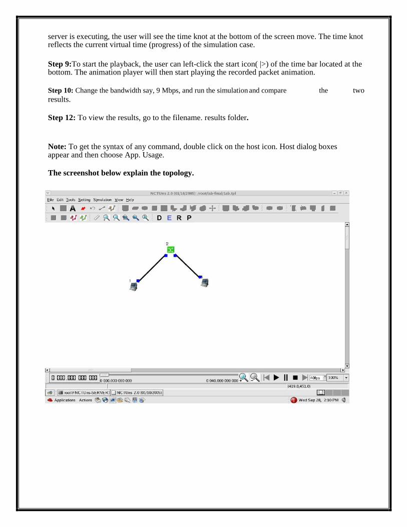
server is executing, the user will see the time knot at the bottom of the screen move. The time knot reflects the current virtual time (progress) of the simulation case.

Step 9:To start the playback, the user can left-click the start icon( |>) of the time bar located at the bottom. The animation player will then start playing the recorded packet animation.

Step 10: Change the bandwidth say, 9 Mbps, and run the simulation and compare the two

results.

Step 12: To view the results, go to the filename. results folder.

Note: To get the syntax of any command, double click on the host icon. Host dialog boxes appear and then choose App. Usage.

The screenshot below explain the topology.

EXPERIMENT 2

Simulate the transmission of ping messages over a network topology consisting of 6 nodes and find the number of packets dropped due to congestion.

STEPS:

Step 1: Click on the subnet icon on the toolbar and then click on the screen of the

working window.

Step 2: Select the required number of hosts and a suitable radius between the host and the

switch.

Step 3: In the edit mode, get the IP address of one of the hosts say, host 1 and then for

the other host say, host2 set the drop packet and no: of collisions statistics

as described in the earlier experiments.

Step 4: Now run the simulation.

Step 5: Now click on any one of the hosts and click on command console and ping the

destination node.

ping IP Address of the host

Note: The no: of drop packets are obtained only when the traffic is more in the

network. For checking the no of packets dropped press ctrl+C

The screenshot of the topology is shown below:

EXPERIMENT 3

Simulate an Ethernet LAN using N nodes and set multiple traffic nodes and plot congestion window for different source/destination.

STEPS:

Step 1: Connect one set of hosts with a hub and another set of hosts also through a hub and connect these two hubs through a switch. This forms an Ethernet LAN.

Step 2: Setup multiple traffic connections between the hosts on one hub and hosts on another hub using the following command:

stcp [-p port] [-l writesize] hostIPaddr rtcp [-p port] [-l readsize]

Step 3: Setup the collision log at the destination hosts in the MAC layer as described in the earlier experiments.

Step 4: To plot the congestion window go to Menu->Tools->Plot Graph->File->open- >filename.results->filename.coll.log

Step 5: View the results in the filename.results.

The screenshot of the topology is shown below:

EXPERIMENT 4

Simulate simple ESS and with transmitting nodes in wireless LAN by simulation

and determine the performance with respect to transmission of packets.

STEPS:

Step 1: Connect a host and two WLAN access points to a router.

Step 2: Setup multiple mobile nodes around the two WLAN access points and set the path for each mobile node.

Step 3: Setup a ttcp connection between the mobile nodes and host using the following command:

Mobile

Host 1

ttcp –t –u –s –p 3000 IPAddrOf Receiver

Mobile

Host 1

ttcp –t –u –s –p 4000 IPAddrOf Receiver

Host(Receiver)

ttcp –r –u –s –p

3000 ttcp –r –u

–s –p 4000

Step 4: Setup the input throughput log at the destination host.

Step 5: To set the transmission range go to Menu->Settings->WLAN mobile node->Show

transmission range.

Step 5: View the results in the filename. results.

Screenshot

EXPERIMENT 5 &6

5. Implement and study the performance of GSM on NS2/NS3 (Using MAC

layer) or equivalent environment. 6. Implement and study the performance of CDMA on NS2/NS3 (Using stack

called Call net) or equivalent environment.

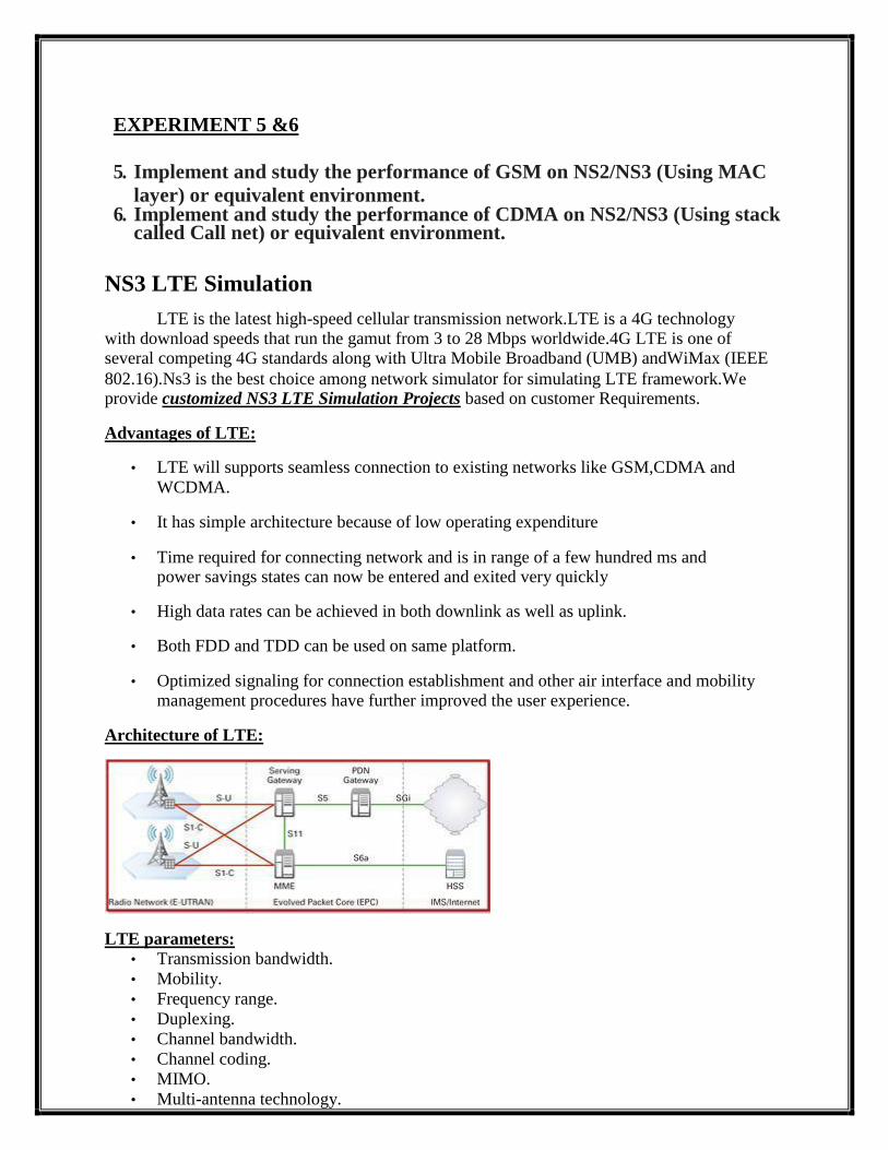
NS3 LTE Simulation

LTE is the latest high-speed cellular transmission network.LTE is a 4G technology with download speeds that run the gamut from 3 to 28 Mbps worldwide.4G LTE is one of several competing 4G standards along with Ultra Mobile Broadband (UMB) andWiMax (IEEE 802.16).Ns3 is the best choice among network simulator for simulating LTE framework.We provide customized NS3 LTE Simulation Projects based on customer Requirements.

Advantages of LTE:

• LTE will supports seamless connection to existing networks like GSM,CDMA and

WCDMA.

• It has simple architecture because of low operating expenditure

• Time required for connecting network and is in range of a few hundred ms and power savings states can now be entered and exited very quickly

• High data rates can be achieved in both downlink as well as uplink.

• Both FDD and TDD can be used on same platform.

• Optimized signaling for connection establishment and other air interface and mobility management procedures have further improved the user experience.

Architecture of LTE:

LTE parameters:

• Transmission bandwidth.

• Mobility.

• Frequency range.

• Duplexing.

• Channel bandwidth.

• Channel coding.

• MIMO.

• Multi-antenna technology.

Sample code for LTE:

#include "ns3/core-module.h"

#include "ns3/network-module.h"

#include "ns3/mobility-module.h"

#include "ns3/lte-module.h" #include "ns3/config-store-module.h"

using namespace ns3;

int main (int argc, char *argv[])

{

CommandLine cmd;

cmd.Parse (argc, argv);

ConfigStore inputConfig;

inputConfig.ConfigureDefaults ();

cmd.Parse (argc, argv);

Ptr<LteHelper> lteHelper = CreateObject<LteHelper> ();

lteHelper->SetAttribute ("PathlossModel", StringValue

("ns3::FriisSpectrumPropagationLossModel"));

NodeContainer enbNodes;

NodeContainer ueNodes;

enbNodes.Create (1);

ueNodes.Create (3);

MobilityHelper mobility; mobility.SetMobilityModel ("ns3::ConstantPositionMobilityModel");

mobility.Install (enbNodes); mobility.SetMobilityModel ("ns3::ConstantPositionMobilityModel");

mobility.Install (ueNodes);

NetDeviceContainer enbDevs;

NetDeviceContainer ueDevs; enbDevs = lteHelper->InstallEnbDevice (enbNodes); ueDevs = lteHelper->InstallUeDevice (ueNodes); lteHelper->Attach (ueDevs, enbDevs.Get (0)); enum EpsBearer::Qci q = EpsBearer::GBR_CONV_VOICE;

EpsBearer bearer (q);

lteHelper->ActivateDataRadioBearer (ueDevs, bearer);

Simulator::Stop (Seconds (0.5));

lteHelper->EnablePhyTraces ();

lteHelper->EnableMacTraces ();

lteHelper->EnableRlcTraces ();

double distance_temp [] = { 1000,1000,1000};

std::vector<double> userDistance;

userDistance.assign (distance_temp, distance_temp + 3);

for (int i = 0; i < 3; i++) {

Ptr<ConstantPositionMobilityModel> mm = ueNodes.Get

(i)->GetObject<ConstantPositionMobilityModel> (); mm-

>SetPosition (Vector (userDistance[i], 0.0, 0.0)); }

Simulator::Run ();

Simulator::Destroy ();

return 0;

}

Part B

EXPERIMENT 7

Write a program for error detecting code using CRC-CCITT (16- bits).

Theory

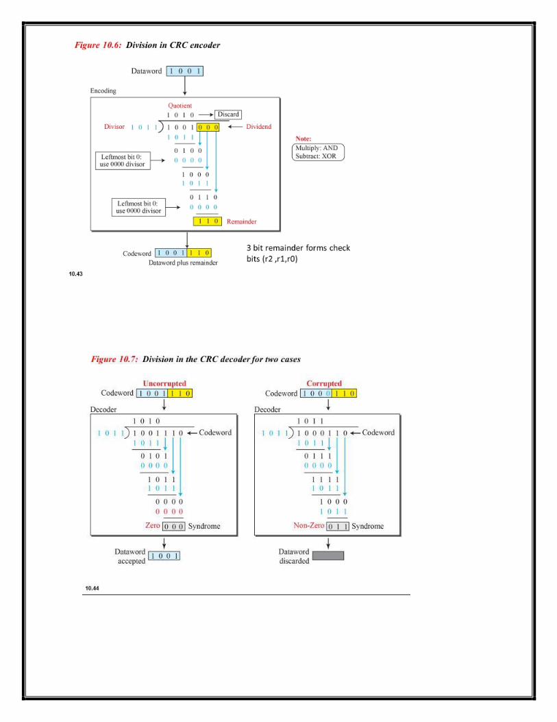
The cyclic redundancy check, or CRC, is a technique for detecting errors in digital data, but not

for making corrections when errors are detected. It is used primarily in data transmission.

In the CRC method, a certain number of check bits, often called a checksum, are appended to the

message being transmitted. The receiver can determine whether or not the check bits agree with the data, to

ascertain with a certain degree of probability whether or not an error occurred in transmission.

It does error checking via polynomial division. In general, a bit string

b b

b …b b b n-1 n-2 n-3

2 1 0 As

bn-1Xn-1

+ bn-2 Xn-2

+ bn-3 Xn-3

+ …b2 X2

+ b1 X1

+ b0

Ex: - 10001000000100001

As

X16

+ X12

+ X5

+1

All computations are done in modulo 2

Algorithm:-

1. Given a bit string, append 0S

to the end of it (the number of 0s is the same as the degree of

the generator polynomial) let B(x) be the polynomial corresponding to B. 2. Divide B(x) by some agreed on polynomial G(x) (generator polynomial) and determine the

remainder R(x). This division is to be done using Modulo 2 Division.

3. Define T(x) = B(x) –R(x)

(T(x)/G(x) => remainder 0)

4. Transmit T, the bit string corresponding to T(x). 5. Let T’ represent the bit stream the receiver gets and T’(x) the associated polynomial. The receiver

divides T1(x) by G(x). If there is a 0 remainder, the receiver concludes T = T’ and no error occurred otherwise, the receiver concludes an error occurred and requires a retransmission.

Program:

import java.io.*;

class crc_gen

{

public static void main(String args[]) throws IOException

{

BufferedReader br=new BufferedReader(new InputStreamReader(System.in));

int[] data;

int[] div;

int[] divisor;

int[] rem;

int[] crc;

int data_bits, divisor_bits, tot_length;

System.out.println("Enter number of data bits : ");

data_bits=Integer.parseInt(br.readLine());

data=new int[data_bits];

System.out.println("Enter data bits : ");

for(int i=0; i<data_bits; i++)

data[i]=Integer.parseInt(br.readLine());

System.out.println("Enter number of bits in divisor : ");

divisor_bits=Integer.parseInt(br.readLine());

divisor=new int[divisor_bits];

System.out.println("Enter Divisor bits : ");

for(int i=0; i<divisor_bits; i++)

divisor[i]=Integer.parseInt(br.readLine());

/* System.out.print("Data bits are : ");

for(int i=0; i< data_bits; i++)

System.out.print(data[i]);

System.out.println();

System.out.print("divisor bits are : ");

for(int i=0; i< divisor_bits; i++)

System.out.print(divisor[i]);

System.out.println();

*/ tot_length=data_bits+divisor_bits-1;

div=new int[tot_length];

rem=new int[tot_length];

crc=new int[tot_length];

/*------------------ CRC GENERATION-----------------------*/

for(int i=0;i<data.length;i++)

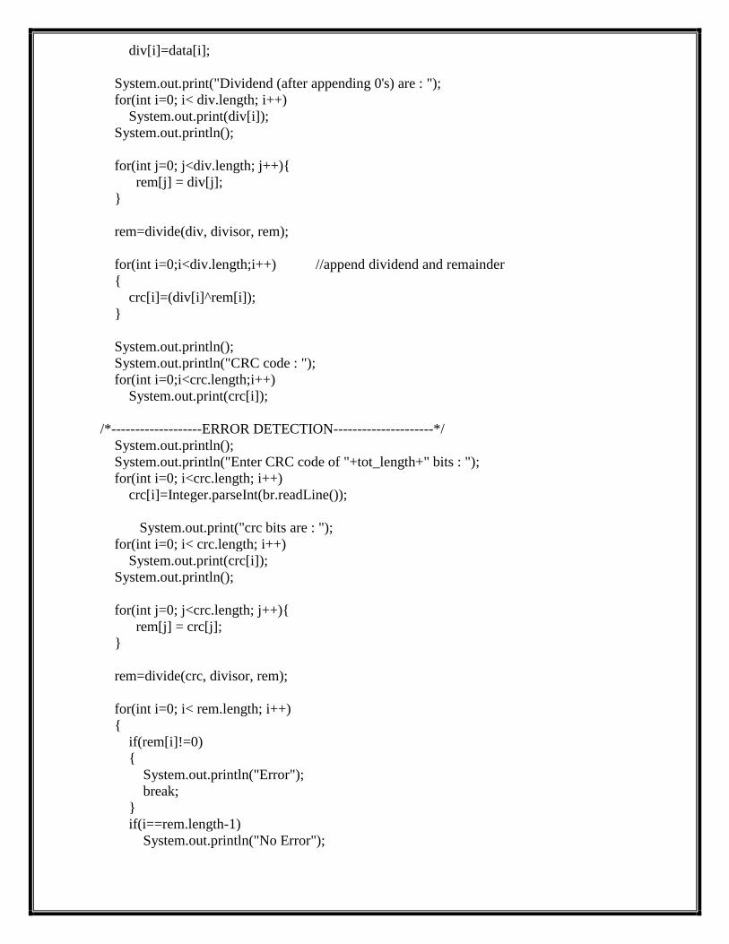
div[i]=data[i];

System.out.print("Dividend (after appending 0's) are : ");

for(int i=0; i< div.length; i++)

System.out.print(div[i]);

System.out.println();

for(int j=0; j<div.length; j++){

rem[j] = div[j];

}

rem=divide(div, divisor, rem);

for(int i=0;i<div.length;i++) //append dividend and remainder

{

crc[i]=(div[i]^rem[i]);

}

System.out.println();

System.out.println("CRC code : ");

for(int i=0;i<crc.length;i++)

System.out.print(crc[i]);

/*-------------------ERROR DETECTION---------------------*/

System.out.println();

System.out.println("Enter CRC code of "+tot_length+" bits : ");

for(int i=0; i<crc.length; i++)

crc[i]=Integer.parseInt(br.readLine());

System.out.print("crc bits are : ");

for(int i=0; i< crc.length; i++)

System.out.print(crc[i]);

System.out.println();

for(int j=0; j<crc.length; j++){

rem[j] = crc[j];

}

rem=divide(crc, divisor, rem);

for(int i=0; i< rem.length; i++)

{

if(rem[i]!=0)

{

System.out.println("Error");

break;

}

if(i==rem.length-1)

System.out.println("No Error");

}

System.out.println("THANK YOU.... :)");

}

static int[] divide(int div[],int divisor[], int rem[])

{

int cur=0;

while(true)

{

for(int i=0;i<divisor.length;i++)

rem[cur+i]=(rem[cur+i]^divisor[i]);

while(rem[cur]==0 && cur!=rem.length-1)

cur++;

if((rem.length-cur)<divisor.length)

break;

}

return rem;

}

}

OUTPUT :

run:

Enter number of data bits :

7

Enter data bits :

1

0

1

1

0

0

1

Enter number of bits in divisor :

3

Enter Divisor bits :

1

0

1

Dividend (after appending 0's) are : 101100100

CRC code :

101100111

Enter CRC code of 9 bits :

1

0

1

1

0

0

1

0

1

crc bits are : 101100101

Error

THANK YOU.... :)

BUILD SUCCESSFUL (total time: 1 minute 34 seconds)

EXPERIMENT 8

Write a program to find the shortest path between vertices using bellman-

ford algorithm.

Theory

Routing algorithm is a part of network layer software which is responsible for deciding which output line an incoming packet should be transmitted on. If the subnet uses datagram internally, this decision must be made for every arriving data packet since the best route may have changed since last time. If the subnet uses virtual circuits internally, routing decisions are made only when a new established route is being set up. The latter case is sometimes called session routing, because a route remains in force for an entire user session (e.g., login session at a terminal or a file).

Routing algorithms can be grouped into two major classes: adaptive and nonadaptive. Nonadaptive

algorithms do not base their routing decisions on measurement or estimates of current traffic and topology.

Instead, the choice of route to use to get from I to J (for all I and J) is compute in advance, offline, and

downloaded to the routers when the network ids booted. This procedure is sometime called static routing.

Adaptive algorithms, in contrast, change their routing decisions to reflect changes in the topology, and usually the traffic as well. Adaptive algorithms differ in where they get information (e.g., locally, from adjacent routers, or from all routers), when they change the routes (e.g., every ■T sec, when the load changes, or when the topology changes), and what metric is used for optimization (e.g., distance, number of hops, or estimated transit time).

Two algorithms in particular, distance vector routing and link state routing are the most popular. Distance vector routing algorithms operate by having each router maintain a table (i.e., vector) giving the best known distance to each destination and which line to get there. These tables are updated by exchanging information with the neighbors.

The distance vector routing algorithm is sometimes called by other names, including the distributed Bellman-Ford routing algorithm and the Ford-Fulkerson algorithm, after the researchers who developed it (Bellman, 1957; and Ford and Fulkerson, 1962). It was the original ARPANET routing algorithm and was also used in the Internet under the RIP and in early versions of DECnet and Novell’s IPX. AppleTalk and Cisco routers use improved distance vector protocols.

In distance vector routing, each router maintains a routing table indexed by, and containing one entry

for, each router in subnet. This entry contains two parts: the preferred out going line to use for that destination, and an estimate of the time or distance to that destination. The metric used might be number of hops, time delay in milliseconds, total number of packets queued along the path, or something similar.

The router is assumed to know the “distance” to each of its neighbor. If the metric is hops, the distance is just one hop. If the metric is queue length, the router simply examines each queue. If the metric is delay, the router can measure it directly with special ECHO packets hat the receiver just time stamps and sends back as fast as possible.

The Count to Infinity Problem.

Distance vector routing algorithm reacts rapidly to good news, but leisurely to bad news. Consider a router whose best

route to destination X is large. If on the next exchange neighbor. A suddenly reports a short delay to X, the router just switches over to using the line to A to send traffic to X. In one vector exchange, the good news is processed.

To see how fast good news propagates, consider the five node (linear) subnet of following figure, where the delay

metric is the number of hops. Suppose A is down initially and all the other routers know this. In other words, they have all recorded the delay to A as infinity.

A B C D E A B C D E

_____ _____ _____ _____ _____ _____ _____ _____

∞ ∞ ∞ ∞ Initially 1 2 3 4 Initially

1 ∞ ∞ ∞ After 1 exchange 3 2 3 4 After 1 exchange

1 2 ∞ ∞ After 2 exchange 3 3 3 4 After 2 exchange

1 2 3 ∞ After 3 exchange 5 3 5 4 After 3 exchange

1 2 3 4 After 4 exchange 5 6 5 6 After 4 exchange

7 6 7 6 After 5 exchange

7 8 7 8 After 6 exchange

:

∞ ∞ ∞ ∞

Many ad hoc solutions to the count to infinity problem have been proposed in the literature, each one more

complicated and less useful than the one before it. The split horizon algorithm works the same way as distance vector

routing, except that the distance to X is not reported on line that packets for X are sent on (actually, it is reported as

infinity). In the initial state of right figure, for example, C tells D the truth about distance to A but C tells B that its

distance to A is infinite. Similarly, D tells the truth to E but lies to C.

Each node x begins with Dx(y), an estimate of the cost of the least-cost path from itself to node y, for all

nodes in N. Let Dx = [Dx(y): y in N] be node x’s distance vector, which is the vector of cost estimates from

x to all other nodes, y, in N. With the DV algorithm, each node x maintains the following routing information: • For each neighbor v, the cost c(x,v) from x to directly attached neighbor, v • Node x’s distance vector, that is, Dx = [Dx(y): y in N], containing x’s estimate of its cost to all destinations, y, in N • The distance vectors of each of its neighbors, that is, Dv = [Dv(y): y in N] for each neighbor v of

x

Program:

import java.util.Scanner;

public class bellmanford

{

private int distances[];

private int numberofvertices;

public static final int MAX_VALUE = 999;

public bellmanford(int numberofvertices)

{

this.numberofvertices = numberofvertices;

distances = new int[numberofvertices + 1];

}

public void BellmanFordEvaluation(int source, int destination,

int adjacencymatrix[][])

{

for (int node = 1; node <= numberofvertices; node++)

{

distances[node] = MAX_VALUE;

}

distances[source] = 0;

for (int node = 1; node <= numberofvertices - 1; node++)

{

for (int sourcenode = 1; sourcenode <= numberofvertices; sourcenode++)

{

for (int destinationnode = 1; destinationnode <= numberofvertices; destinationnode++)

{

if (adjacencymatrix[sourcenode][destinationnode] != MAX_VALUE)

{

if (distances[destinationnode] > distances[sourcenode]

+ adjacencymatrix[sourcenode][destinationnode])

distances[destinationnode] = distances[sourcenode]

+ adjacencymatrix[sourcenode][destinationnode];

}

}

}

}

for (int sourcenode = 1; sourcenode <= numberofvertices; sourcenode++)

{

for (int destinationnode = 1; destinationnode <= numberofvertices; destinationnode++)

{

if (adjacencymatrix[sourcenode][destinationnode] != MAX_VALUE)

{

if (distances[destinationnode] > distances[sourcenode]

+ adjacencymatrix[sourcenode][destinationnode])

System.out

.println("The Graph contains negative egde cycle");

}

}

}

for (int vertex = 1; vertex <= numberofvertices; vertex++)

{

if (vertex == destination)

System.out.println("distance of source " + source + " to "

+ vertex + " is " + distances[vertex]);

}

}

public static void main(String... arg)

{

int numberofvertices = 0;

int source, destination;

Scanner scanner = new Scanner(System.in);

System.out.println("Enter the number of vertices");

numberofvertices = scanner.nextInt();

int adjacencymatrix[][] = new int[numberofvertices + 1][numberofvertices + 1];

System.out.println("Enter the adjacency matrix");

for (int sourcenode = 1; sourcenode <= numberofvertices; sourcenode++)

{

for (int destinationnode = 1; destinationnode <= numberofvertices; destinationnode++)

{

adjacencymatrix[sourcenode][destinationnode] = scanner

.nextInt();

if (sourcenode == destinationnode)

{

adjacencymatrix[sourcenode][destinationnode] = 0;

continue;

}

if (adjacencymatrix[sourcenode][destinationnode] == 0)

{

adjacencymatrix[sourcenode][destinationnode] = MAX_VALUE;

}

}

}

System.out.println("Enter the source vertex");

source = scanner.nextInt();

System.out.println("Enter the destination vertex: ");

destination = scanner.nextInt();

bellmanford bellmanford = new bellmanford(numberofvertices);

bellmanford.BellmanFordEvaluation(source, destination, adjacencymatrix);

scanner.close();

}

}

OUTPUT:

run:

Enter the number of vertices

6

Enter the adjacency matrix

0 4 0 0 -1 0

0 0 -1 0 -2 0

0 0 0 0 0 0

0 0 0 0 0 0

0 0 0 -5 0 3

0 0 0 0 0 0

Enter the source vertex

1

Enter the destination vertex:

4

Distance of source 1 to 4 is -6

BUILD SUCCESSFUL (total time: 53 seconds)

EXPERIMENT 9

Using TCP/IP sockets, write a client – server program to make the client send the

file name and to make the server send back the contents of the requested file if

present. Implement the above program using as message queues or FIFOs as IPC

channels.

TCP Socket

TCP is a connection-oriented protocol. This means that before the client and server can start to send

data to each other, they first need to handshake and establish a TCP connection. One end of the TCP

connection is attached to the client socket and the other end is attached to a server socket. When creating

the TCP connection, we associate with it the client socket address (IPaddress and port number) and the

server socket address (IPaddress and port number). With the TCP connection established, when one side

wants to send data to the other side, it just drops the data into the TCP connection via its socket.

With the server process running, the client process can initiate a TCP connection to the server. This

is done in the client program by creating a TCP socket. When the client creates its TCP socket, it specifies

the address of the welcoming socket in the server, namely, the IP address of the server host and the port

number of the socket. After creating its socket, the client initiates a three-way handshake and establishes a

TCP connection with the server.

Example:

Server Program

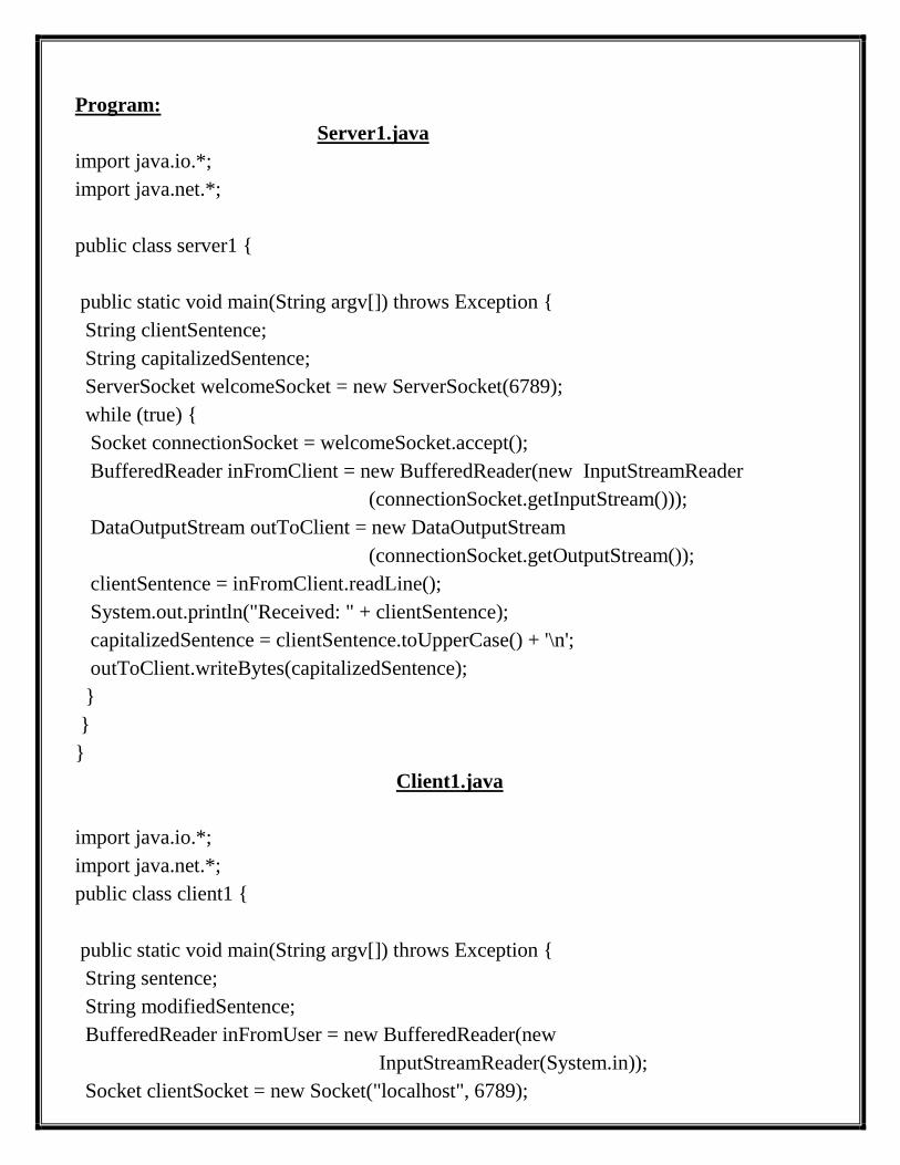
Program:

Server1.java

import java.io.*;

import java.net.*;

public class server1 {

public static void main(String argv[]) throws Exception {

String clientSentence;

String capitalizedSentence;

ServerSocket welcomeSocket = new ServerSocket(6789);

while (true) {

Socket connectionSocket = welcomeSocket.accept();

BufferedReader inFromClient = new BufferedReader(new InputStreamReader

(connectionSocket.getInputStream()));

DataOutputStream outToClient = new DataOutputStream

(connectionSocket.getOutputStream());

clientSentence = inFromClient.readLine();

System.out.println("Received: " + clientSentence);

capitalizedSentence = clientSentence.toUpperCase() + '\n';

outToClient.writeBytes(capitalizedSentence);

}

}

}

Client1.java

import java.io.*;

import java.net.*;

public class client1 {

public static void main(String argv[]) throws Exception {

String sentence;

String modifiedSentence;

BufferedReader inFromUser = new BufferedReader(new

InputStreamReader(System.in));

Socket clientSocket = new Socket("localhost", 6789);

DataOutputStream outToServer = new

DataOutputStream (clientSocket.getOutputStream());

BufferedReader inFromServer = new BufferedReader(new InputStreamReader

(clientSocket.getInputStream()));

sentence = inFromUser.readLine();

outToServer.writeBytes(sentence + '\n');

modifiedSentence = inFromServer.readLine();

System.out.println("FROM SERVER: " + modifiedSentence);

clientSocket.close();

}

}

OUTPUT: run both Server1.java & Client1.java files

Client1 side

run:

hi, good Morning ,are you fine?

FROM SERVER: HI, GOOD MORNING ,ARE YOU FINE?

BUILD SUCCESSFUL (total time: 43 seconds)

Server1 side

run:

Received: hi, good Morning ,are you fine?

EXPERIMENT 10

Write a program on datagram socket for client/server to display the messages on

client side, typed at the server side.

Using User Datagram Protocol, Applications can send data/message to the other hosts without prior

communications or channel or path. This means even if the destination host is not available, application can send data. There is no guarantee that the data is received in the other side. Hence it's not a reliable service.

UDP is appropriate in places where delivery of data doesn't matters during data transition.

Server.java

Program:

import java.io.*;

import java.net.*;

public class server

{

public static void main(String args[]) throws Exception

{

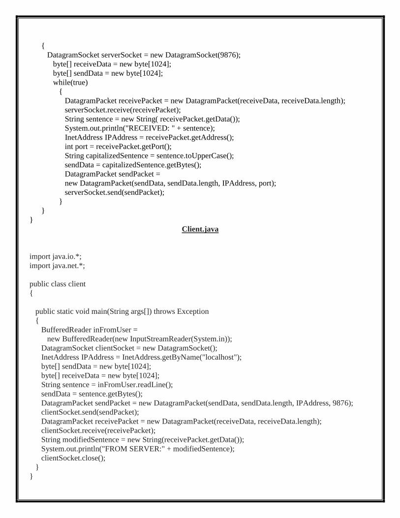
DatagramSocket serverSocket = new DatagramSocket(9876);

byte[] receiveData = new byte[1024];

byte[] sendData = new byte[1024];

while(true)

{

DatagramPacket receivePacket = new DatagramPacket(receiveData, receiveData.length);

serverSocket.receive(receivePacket);

String sentence = new String( receivePacket.getData());

System.out.println("RECEIVED: " + sentence);

InetAddress IPAddress = receivePacket.getAddress();

int port = receivePacket.getPort();

String capitalizedSentence = sentence.toUpperCase();

sendData = capitalizedSentence.getBytes();

DatagramPacket sendPacket =

new DatagramPacket(sendData, sendData.length, IPAddress, port);

serverSocket.send(sendPacket);

}

}

}

Client.java

import java.io.*;

import java.net.*;

public class client

{

public static void main(String args[]) throws Exception

{

BufferedReader inFromUser =

new BufferedReader(new InputStreamReader(System.in));

DatagramSocket clientSocket = new DatagramSocket();

InetAddress IPAddress = InetAddress.getByName("localhost");

byte[] sendData = new byte[1024];

byte[] receiveData = new byte[1024];

String sentence = inFromUser.readLine();

sendData = sentence.getBytes();

DatagramPacket sendPacket = new DatagramPacket(sendData, sendData.length, IPAddress, 9876);

clientSocket.send(sendPacket);

DatagramPacket receivePacket = new DatagramPacket(receiveData, receiveData.length);

clientSocket.receive(receivePacket);

String modifiedSentence = new String(receivePacket.getData());

System.out.println("FROM SERVER:" + modifiedSentence);

clientSocket.close();

}

}

OUTPUT: run both server.java & client.java files

Client side

run:

hello,how r u

FROM SERVER:HELLO,HOW R U

Server side

RECEIVED: hello,how r u

EXPERIMENT 11

Write a program for simple RSA algorithm to encrypt and decrypt the data.

Theory

Cryptography has a long and colorful history. The message to be encrypted, known as the plaintext, are transformed by a function that is parameterized by a key. The output of the encryption process, known as the ciphertext, is then transmitted, often by messenger or radio. The enemy, or intruder, hears and accurately copies down the complete ciphertext. However, unlike the intended recipient, he does not know the decryption key and so cannot decrypt the ciphertext easily. The art of breaking ciphers is called cryptanalysis the art of devising ciphers (cryptography) and breaking them (cryptanalysis) is collectively known as cryptology.

There are several ways of classifying cryptographic algorithms. They are generally categorized based on

the number of keys that are employed for encryption and decryption, and further defined by their application and use. The three types of algorithms are as follows:

1. Secret Key Cryptography (SKC): Uses a single key for both encryption and decryption. It is also known as symmetric cryptography.

2. Public Key Cryptography (PKC): Uses one key for encryption and another for decryption. It is also known as asymmetric cryptography.

3. Hash Functions: Uses a mathematical transformation to irreversibly "encrypt" information

Public-key cryptography has been said to be the most significant new development in cryptography.

Modern PKC was first described publicly by Stanford University professor Martin Hellman and graduate student Whitfield Diffie in 1976. Their paper described a two-key crypto system in which two parties could engage in a secure communication over a non-secure communications channel without having to share a secret key.

Generic PKC employs two keys that are mathematically related although knowledge of one key does not allow someone to easily determine the other key. One key is used to encrypt the plaintext and the other key is used to decrypt the ciphertext. The important point here is that it does not matter which key is applied first, but that both keys are required for the process to work. Because pair of keys is required, this approach is also called asymmetric cryptography.

In PKC, one of the keys is designated the public key and may be advertised as widely as the owner

wants. The other key is designated the private key and is never revealed to another party. It is straight forward to send messages under this scheme.

The RSA algorithm is named after Ron Rivest, Adi Shamir and Len Adleman, who invented it in 1977.

The RSA algorithm can be used for both public key encryption and digital signatures. Its security is based on the difficulty of factoring large integers. Algorithm

1. Generate two large random primes, P and Q, of approximately equal size.

2. Compute N = P x Q

3. Compute Z = (P-1) x (Q-1).

4. Choose an integer E, 1 < E < Z, such that GCD (E, Z) = 1 5. Compute the secret exponent D, 1 < D < Z, such that E x D ≡ 1 (mod Z) 6. The public key is (N, E) and the private key is (N, D).

Note: The values of P, Q, and Z should also be kept secret. The message is encrypted using public key and decrypted using private key.

An example of RSA encryption

1. Select primes P=11, Q=3. 2. N = P x Q = 11 x 3 = 33 Z = (P-1) x (Q-1) = 10 x 2 = 20 3. Lets choose E=3

Check GCD(E, P-1) = GCD(3, 10) = 1 (i.e. 3 and 10 have no common factors except 1), and check GCD(E, Q-1) = GCD(3, 2) = 1 therefore GCD(E, Z) = GCD(3, 20) = 1

4. Compute D such that E x D ≡ 1 (mod Z) compute D = E

^-1 mod Z = 3

^-1 mod 20

find a value for D such that Z divides ((E xD)-1) find D such that 20 divides 3D-1.

Simple testing (D = 1, 2, ...) gives D = 7

Check: (E x D)-1 = 3.7 - 1 = 20, which is divisible by Z.

5. Public key = (N, E) = (33, 3) Private key = (N, D) = (33, 7).

Now say we want to encrypt the message m = 7,

Cipher code = M^E

mod N = 7^3

mod 33 = 343 mod 33 =13. Hence the ciphertext c = 13.

To check decryption we compute Message’ = C

^D mod N = 13

^7 mod 33= 7.

Note that we don't have to calculate the full value of 13 to the power 7 here. We can make use of the fact that a = bc mod n = (b mod n).(c mod n) mod n so we can break down a potentially large number into its components and combine the results of easier, smaller calculations to calculate the final value.

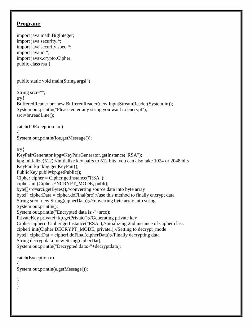
Program:

import java.math.BigInteger;

import java.security.*;

import java.security.spec.*;

import java.io.*;

import javax.crypto.Cipher;

public class rsa {

public static void main(String args[])

{

String srci="";

try{

BufferedReader br=new BufferedReader(new InputStreamReader(System.in));

System.out.println("Please enter any string you want to encrypt");

srci=br.readLine();

}

catch(IOException ioe)

{

System.out.println(ioe.getMessage());

}

try{

KeyPairGenerator kpg=KeyPairGenerator.getInstance("RSA");

kpg.initialize(512);//initialize key pairs to 512 bits ,you can also take 1024 or 2048 bits

KeyPair kp=kpg.genKeyPair();

PublicKey publi=kp.getPublic();

Cipher cipher = Cipher.getInstance("RSA");

cipher.init(Cipher.ENCRYPT_MODE, publi);

byte[]src=srci.getBytes();//converting source data into byte array

byte[] cipherData = cipher.doFinal(src);//use this method to finally encrypt data

String srco=new String(cipherData);//converting byte array into string

System.out.println();

System.out.println("Encrypted data is:-"+srco);

PrivateKey privatei=kp.getPrivate();//Generating private key

Cipher cipheri=Cipher.getInstance("RSA");//Intializing 2nd instance of Cipher class

cipheri.init(Cipher.DECRYPT_MODE, privatei);//Setting to decrypt_mode

byte[] cipherDat = cipheri.doFinal(cipherData);//Finally decrypting data

String decryptdata=new String(cipherDat);

System.out.println("Decrypted data:-"+decryptdata);

}

catch(Exception e)

{

System.out.println(e.getMessage());

}

}

}

OUTPUT:-

Please enter any string you want to encrypt

hello

Encrypted data is:- i� �������`>��a�:�ʪ

Decrypted data:-hello

BUILD SUCCESSFUL (total time: 12 seconds)

EXPERIMENT 12

Write a program for congestion control using leaky bucket algorithm. Theory

The congesting control algorithms are basically divided into two groups: open loop and closed loop. Open loop solutions attempt to solve the problem by good design, in essence, to make sure it does not occur in the first place. Once the system is up and running, midcourse corrections are not made. Open loop algorithms are further divided into ones that act at source versus ones that act at the destination.

In contrast, closed loop solutions are based on the concept of a feedback loop if there is any congestion. Closed loop algorithms are also divided into two sub categories: explicit feedback and implicit feedback. In explicit feedback algorithms, packets are sent back from the point of congestion to warn the source. In implicit algorithm, the source deduces the existence of congestion by making local observation, such as the time needed for acknowledgment to come back.

The presence of congestion means that the load is (temporarily) greater than the resources (in part of the

system) can handle. For subnets that use virtual circuits internally, these methods can be used at the network layer.

Another open loop method to help manage congestion is forcing the packet to be transmitted at a more

predictable rate. This approach to congestion management is widely used in ATM networks and is called traffic shaping.

The other method is the leaky bucket algorithm. Each host is connected to the network by an interface

containing a leaky bucket, that is, a finite internal queue. If a packet arrives at the queue when it is full, the packet is discarded. In other words, if one or more process are already queued, the new packet is unceremoniously discarded. This arrangement can be built into the hardware interface or simulate d by the host operating system. In fact it is nothing other than a single server queuing system with constant service time.

The host is allowed to put one packet per clock tick onto the network. This mechanism turns an uneven flow

of packet from the user process inside the host into an even flow of packet onto the network, smoothing out bursts and greatly reducing the chances of congestion.

Program: import java.util.*;

public class leakybucketalgorithm {

public static void main(String[] args)

{

Scanner my = new Scanner(System.in);

int no_groups,bucket_size;

System.out.print("\n Enter the bucket size : \t");

bucket_size = my.nextInt();

System.out.print("\n Enter the no of groups : \t");

no_groups = my.nextInt();

int no_packets[] = new int[no_groups];

int in_bw[] = new int[no_groups];

int out_bw,reqd_bw=0,tot_packets=0;

for(int i=0;i<no_groups;i++)

{

System.out.print("\n Enter the no of packets for group " + (i+1) + "\t");

no_packets[i] = my.nextInt();

System.out.print("\n Enter the input bandwidth for the group " + (i+1) + "\t");

in_bw[i] = my.nextInt();

if((tot_packets+no_packets[i])<=bucket_size)

{

tot_packets += no_packets[i];

}

else

{

do

{

System.out.println(" Bucket Overflow ");

System.out.println(" Enter value less than " + (bucket_size-tot_packets));

no_packets[i] = my.nextInt();

}while((tot_packets+no_packets[i])>bucket_size);

tot_packets += no_packets[i];

}

reqd_bw += (no_packets[i]*in_bw[i]);

}

System.out.println("\nThe total required bandwidth is " + reqd_bw);

System.out.println("Enter the output bandwidth ");

out_bw = my.nextInt();

int temp=reqd_bw;

int rem_pkts = tot_packets;

while((out_bw<=temp)&&(rem_pkts>0))

{

System.out.println("Data Sent \n" + (--rem_pkts) + " packets remaining");

System.out.println("Remaining Bandwidth " + (temp -= out_bw));

if((out_bw>temp)&&(rem_pkts>0))

System.out.println(rem_pkts + " packet(s) discarded due to insufficient bandwidth");

}

}

}

OUTPUT:-

Enter the bucket size : 10

Enter the no of groups: 2

Enter the no of packets for group 1 3

Enter the input bandwidth for the group 1 4

Enter the no of packets for group 2 4

Enter the input bandwidth for the group 2 3

The total required bandwidth is 24

Enter the output bandwidth

6

Data Sent

6 packets remaining

Remaining Bandwidth 18

Data Sent

5 packets remaining

Remaining Bandwidth 12

Data Sent

4 packets remaining

Remaining Bandwidth 6

Data Sent

3 packets remaining

Remaining Bandwidth 0

3 packet(s) discarded due to insufficient bandwidth

BUILD SUCCESSFUL (total time: 43 seconds)