NASA/TM-2002-211944

ARL-TR-2849

Best PracticesSimulation

for Crash Modeling

Edwin L. Fasanella and Karen E. Jackson

U.S. Army Research Laboratory

Vehicle Technology Directorate

Langley Research Center, Hampton, Virginia

and

October 2002

https://ntrs.nasa.gov/search.jsp?R=20020085101 2018-05-25T09:30:08+00:00Z

The NASA STI Program Office... in Profile

Since its founding, NASA has been dedicatedto the advancement of aeronautics and space science.The NASA Scientific and Technical Information

(STI) Program Office plays a key

part in helping NASA maintain this

important role.

The NASA STI Program Office is operated by

Langley Research Center, the lead center for NASA'sscientific and technical information.

The NASA STI Program Office provides

access to the NASA STI Database, the

largest collection of aeronautical and space

science STI in the world. The Program Officeis also NASA's institutional mechanism for

disseminating the results of its research and

development activities. These results are

published by NASA in the NASA STI Report

Series, which includes the following report

types:

TECHNICAL PUBLICATION. Reports of

completed research or a major significant

phase of research that present the results

of NASA programs and include extensive

data or theoretical analysis. Includes compilations

of significant scientific andtechnical data and information deemed

to be of continuing reference value. NASA

counterpart of peer-reviewed formal professional

papers, but having less

stringent limitations on manuscript

length and extent of graphic

presentations.

TECHNICAL MEMORANDUM.

Scientific and technical findings that are

preliminary or of specialized interest,

e.g., quick release reports, working

papers, and bibliographies that containminimal annotation. Does not contain

extensive analysis.

CONTRACTOR REPORT. Scientific and

technical findings by NASA-sponsored

contractors and grantees.

CONFERENCE PUBLICATION.

Collected papers from scientific and

technical conferences, symposia,

seminars, or other meetings sponsored or

co-sponsored by NASA.

SPECIAL PUBLICATION. Scientific,

technical, or historical information from

NASA programs, projects, and missions,

often concerned with subjects having

substantial public interest.

TECHNICAL TRANSLATION. English-

language translations of foreign scientific

and technical material pertinent toNASA's mission.

Specialized services that complement the

STI Program Office's diverse offerings include

creating custom thesauri, building customized

databases, organizing and publishing

research results.., even providing videos.

For more information about the NASA STI

Program Office, see the following:

• Access the NASA STI Program Home

Page at http://www.sti.nasa.gov

• Email your question via the Intemet to

help@sti.nasa.gov

• Fax your question to the NASA STI

Help Desk at (301) 621-0134

• Telephone the NASA STI Help Desk at

(301) 621-0390

Write to:

NASA STI Help Desk

NASA Center for AeroSpace Information7121 Standard Drive

Hanover, MD 21076-1320

NASA/TM-2002-211944

ARL-TR-2849

Best PracticesSimulation

for Crash Modeling

Edwin L. Fasanella and Karen E. Jackson

U.S. Army Research Laboratory

Vehicle Technology Directorate

Langley Research Center, Hampton, Virginia

and

National Aeronautics and

Space Administration

Langley Research Center

Hampton, Virginia 23681-2199

October 2002

The use of trademarks or names of manufacturers in this report is for accurate reporting and does not constitute an

official endorsement, either expressed or implied, of such products or manufacturers by the National Aeronautics and

Space Administration or the U.S. Army.

Available from:

NASA Center for AeroSpace Information (CAS1)

7121 Standard Drive

Hanover, MD 21076-1320

(301) 621-0390

National Technical Information Service (NTIS)

5285 Port Royal Road

Springfield, VA 22161-2171

(703) 605-6000

Best Practices for Crash Modeling and Simulation

I. Abstract

II. Introduction

- Overview of paper

- Objectives

III. General Issues in Developing a Crash Model

- Reference frame and units

- Coordinate frames

- Systems of consistent units

- Geometry Model

- Engineering drawings

- Photographic methods

- Photogrammetric survey- Hand measurements

- Existing finite element model

- Finite element model development

- Mesh generation- Element selection

- Nodal considerations

- Simple beam and spring models- Mechanisms

- Dummy models

- Lagrange and Euler formulations

- Lumped mass- Material model selection

- Material types- Failure

- Damping

- Energy dissipation

- Hysteretic behavior- Initial conditions

- Initial velocities, forces, etc.

- Angular velocity- Contact definitions

- General Contact

- Self-Contact

- Friction

- Contact penalty factor

111

IV. General Issues Related to Model Execution and Analytical Predictions

- Quality checks on model fidelity

- Weight and mass distribution

- Center-of-gravity location

- Misc. (modal vibration data, load test data, etc.)

- Filtering of crash analysis data

- Anomalies and errors in crash analysis data

- Aliasing errors

- Hour glass phenomenon

- Energy considerations

- Velocity considerations

V. Experimental Data and Test-Analysis Correlation

- Test Data Evaluation and Filtering- Electrical anomalies

- Acceleration data

- SAE filtering standards

- Integration as quality check

- Filtering to obtain fundamental acceleration pulse

- Test-Analysis Correlation

- Experimental and analytical data evaluation recommended practice

VI. Conclusions

VII. References

VIII. Appendices: Examples of Full-Scale Crash Simulations and Lessons Learned

Appendix A. Sikorsky ACAP Helicopter Crash Simulation

Appendix B. B737 Fuselage Section Crash Simulation

Appendix C. Lear Fan 2100 Crash Simulation

Appendix D. Crash Simulation of a Composite Fuselage Section with Energy-

Absorbing Seats and Dummies

iv

Best Practices for Crash Modeling and Simulation

Edwin L. Fasanella and Karen E. Jackson

I. Abstract

Aviation safety can be greatly enhanced through application of computer simulations of crash

impact. Unlike automotive impact testing, which is now a routine part of the development

process, crash testing of even small aircraft is infrequently performed due to the high cost of the

aircraft and the myriad of impact conditions that must be considered. Crash simulations are

currently used as an aid in designing, testing, and certifying aircraft components such as seats to

dynamic impact criteria. Ultimately, the goal is to utilize full-scale crash simulations of the

entire aircraft for design evaluation and certification. The objective of this publication is to

describe "best practices" for modeling aircraft impact using explicit nonlinear dynamic finite

element codes such as LS-DYNA, DYNA3D, and MSC.Dytran. Although "best practices" is

somewhat relative, the authors' intent is to help others to avoid some of the common pitfalls in

impact modeling that are not generally documented. In addition, a discussion of experimental

data analysis, digital filtering, and test-analysis correlation is provided. Finally, some examples

of aircraft crash simulations are described in four appendices following the main report.

II. Introduction

Recent advances in computer software and hardware have made possible analysis of complex

nonlinear transient-dynamic events that were nearly impossible to perform just a few years ago.

In addition to the improvement in processing time, the cost of computer hardware has decreased

an order of magnitude in just the last few years. With the continued improvement in computer

workstation speed and the availability of inexpensive computer CPU, memory, and storage, very

large crash impact problems can now be performed on modestly priced desk-top computers that

use operating systems such as LINUX or "Windows". Although the software codes can still be

relatively expensive, as the number of applications and users increase, the cost of software is

expected to decrease, as well.

Aviation safety can be greatly enhanced by the appropriate use of the current generation of

nonlinear explicit transient dynamic codes to predict airframe response during a crash. Unlike

automotive impact testing, which is now a routine part of the development process, crash testing

of even small aircraft is infrequently performed due to the high cost of the aircraft and the

myriad of impact conditions that must be considered. Crash simulations are currently used as an

aid in designing, testing, and certifying aircraft components such as seats to dynamic impact

criteria. Full-scale crash simulations are now being performed as part of aircraft accident

investigations using the semi-empirical finite element code KRASH [1]. Although KRASH

models are relative simple, consisting mainly of beam elements, springs, and dampers; this tool

has enabled crash investigators and designers to better understand and simulate actual aircraft

crash dynamics. The Air Accident Investigation Tool (AAIT) code uses a library of KRASH

models of common aircraft to simplify this process [2].

Theobjectiveof thispaperis to document"bestpractices"for modelingaircraft impactusingexplicitnonlineardynamicfinite element(FE) codessuchasLS-DYNA [3], DYNA3D [4], andMSC.Dytran[5] basedon the authors'pastexperiencein usingthesecodes. Although"bestpractices"is somewhatrelative,theauthors'intentis to helpothersavoidsomeof thecommonpitfallsin impactmodelingthatarenotgenerallydocumented.A basicunderstandingof physics,materialscience,andnonlinearbehavioris assumedandrequired.Nonlinearmodelingrequiresthemodeldeveloperto haveastrategy,to performmanyqualitychecksontheinputdata,andtocarefullyexaminethe outputresultsby performing"sanitychecks." It is bestto validatethemodelthroughcomparisonswith experimentalresults.However,if therearenodatato comparewith, then otherchecksmay have to suffice, suchas carefully observingthe systemandcomponentenergiesfor growthor instabilities.

Thelearningcurveis quite steepin movingfrom a linearstaticstructuralfinite elementcode,suchastheearlierversionsof NASTRAN[6], to anonlineardynamicfiniteelementcode.Afterselectinga simulationcodeand apre- andpost-processingsoftwarepackage,a basiccoursetaughtby thecodevendoris highly recommended.Chooseavendorwith agoodreputationforsoftwaresupportandconsulting.Evenafterbecomingquiteproficientwith thecode,auserwillneedto consultwith the vendoron advancedissuesor to reportsoftwareerrors.Frequently,many assumptionsand simplifications are madeby the developersto make the code runefficiently. Theuserneedsto havea basicunderstandingof theunderlyingassumptionsandlimitationsof theelementsandalgorithmsto besuccessfulin crashmodeling.

Initially, mostof thework onnonlineardynamicfinite elementcodeswasgovernmentfunded;however,the currentcommercialcodesareproprietary.NASA granteda contractto McNeal-SchwendlerCorp.to developtheNASTRAN [6] structuralanalysiscodein the 1960's. Thecodeallowedaircraftdesignersto performstressandmodalanalysesof aircraftstructures.Bytheendof the1960'sandintothe 1970's,NASA andtheFAA fundedGrummanCorporationtodevelopanonlinearstaticstructuralfinite elementcodePlasticAnalysisof Structures(PLANS)[7] andlatertheDynamicCrashAnalysisof Structures(DYCAST)[8] structuralfinite elementcode.Aboutthesametime,theUSArmy fundedtheLockheedCaliforniaCompanyto developa semi-empiricalkinematicfinite elementaircraftcrashanalysiscodecalledKRASH [1]. AlargegroupatLawrenceLivermoreNationalLaboratorieswasfundedbytheUSDepartmentofEnergyin the 1970'sand 1980'sto assemblemuchof the nonlineardynamicstructuralandmaterialknowledgeandto developasuiteof nonlineardynamicfinite elementcodesincludingDYNA2D, DYNA3D [4], NIKE2D, andNIKE3D [9]. The public domainversion of theDYNA3D codewasthe sourcefor a numberof commercialspinoffsincludingLS-DYNA [3],PAMCRASH[10],andMSC.Dytran[5].

Thefollowing sectionsof the paperprovideinformationon developingandexecutinga crashfinite elementmodel,andonperformingqualitychecksof theanalyticalresults. In addition,asectiononexperimentaldataanalysis,filtering, andtest-analysiscorrelationis includedto assistthereaderin determiningwhetherthemodelis adequatefor its intendedpurpose.Finally,sometypical aircraftcrashsimulationsaredescribedin detail in the four appendicesfollowing themainreport.

III. General Issues in Developing a Crash Model

Reference frame and units

Coordinate flames

One of the first steps in developing a model of an aircraft or airframe component is the

development of the geometry. However, even before constructing the geometric model, one

must decide on a coordinate system and a system of units. Quite often, left-handed coordinate

systems are used. For example, in aircraft drawings, body station (BS), water line (WL), and

butt line (BL) dimensions are typically defined using a left-handed system. Finite element

programs do not generally accept a left-handed coordinate system since the equations of vector

algebra are defined in a coordinate system that obeys the "right-hand" rule. Thus, it is important

to choose the origin at an appropriate location and to use a consistent system of the fundamental

physical units of length, time, and mass in defining the model.

Systems of consistent units

The finite element code will accept any units that are input without error checking. Thus, if

engineering units are input using an inconsistent system of units, or a left-handed coordinate

system is used, the results will be flawed. The modeler should be careful with units of force,

mass_ and density, especially when using customary English units commonly used by American

aircraft manufacturers. Using this system, the unit of length is typically the inch, the unit of time

is the second, and the unit of mass is weight in pounds divided by gravity (386.4 in/s2). Note that

weig_h__htin pounds is a force and equals mass times the acceleration of gravity. Density is a

derived unit often specified in pounds per cubic inch. When using consistent English units,

density in lb/in 3 must be divided by the acceleration of gravity (386.4 in/s 2) to obtain the proper

consistent value. For example, the density of a closed-cell polyurethane foam is specified by the

manufacturer as 2.8 lb/ft 3. If using the English-inch system, the density would first be converted

to 0.0016 lb/in 3. Next, the density is divided by the acceleration of gravity (386.4 in/s 2) to

obtain .0000042 lb-s2/in 4, which is the value that must be used in the model. Some typical,

commonly used consistent systems of units are shown in Table I.

Table I Typical Consistent Systems of Units.

Unit

Length

Metric MKS

Meter (m)

English inch

Inch (in)

English foot

Foot (ft)

Time Second (s) Second (s) Second (s)

Mass

ForceKilogram (kg)

Newton (N=kg-m/s 2)

kg/m 3m/s 2

9.8 m/s 2

Pascal (N/m 2)

DensityAcceleration

lb-s2/in

Pound (lb)lb-s2/in 4

in/s 2

386.4 in/s 2

Psi (lb/in 2)

Acceleration of gravityPressure

Slug (lb-s2/ft)

Pound (lb)

Slug/ft 3ft/s 2

32.2 ft/s 2

lb/ft 2

GeometryModelOncethecoordinatesystem,origin,andunitshavebeenselected,thenextstepin thesimulationprocessis to developa geometrymodel. The geometrymodel consistsof points, curves,surfaces,andsolidsthatareusedto definetheshapeof thestructuralcomponents.Thegeometricentitiesareinputinto thepre-processingsoftwarepackage,for exampleMSC.Patran,andwill bediscretizedlaterto formthefiniteelementmodel. Thereareseveralmethodsthatcanbeusedtoobtainthedataneededto createthegeometrymodel. Forexample,thegeometrymodelmaybegenerated from engineering drawings, photographs, photogrammetric survey, handmeasurements,or from an existing finite elementmodel as describedin the followingsubsectionsof thepaper.

Engineering Drawings

If engineering drawings are available in a computer-aided design (CAD) system, it may be

possible to transfer the geometry electronically to the pre-processing software for the finite

element code. Obviously, electronic conversion is a very desirable method to transfer geometry.

Most users of CAD software are familiar with transferring data from one software program to

another. Also, it might be useful to consult with the code developer as it is in the vendor's best

interests to provide advice on portability between different platforms and different software

programs. The Initial Graphics Exchange Specification (IGES) defines a neutral data format that

allows for the digital exchange of information among CAD systems. CAD systems are in use

today in increasing numbers for applications in all phases of the design, analysis, manufacture,

and testing of products. Since it is common practice for a designer to use one supplier's CAD

system and for the contractor and subcontractors to use different systems, there is a need for the

ability to exchange digital data among all CAD systems.

IGES provides a neutral definition and format for the exchange of specific data. Using IGES, a

user can exchange data models in the form of wire frame or solid representations, as well as

surface representations. Applications supported by IGES include traditional engineering

drawings as well as models for analysis and/or various manufacturing functions. In addition to

the general specification, IGES includes application protocols in which the standard is

interpreted to meet discipline specific requirements. IGES is an American National Standard

(ANS), and the latest version of the IGES standard is designated ANS US PRO/IPO- 100-1996.

If the drawings are only available as printed copies, software is available to make the task of

generating electronic data for developing the geometry model easier. Software can be obtained

from vendors such as Trix Systems (wwwArixss'stems.com) that will convert paper drawings to

IGES files. Once IGES files are created, they may be imported into pre-processing software

packages such as MSC.Patran, etc. Without the software, the drawings would have to be

manually converted to points, lines, and surfaces by direct keystroke input into your pre-

processing software package.

Photographic methods

If drawings are not available, photographic methods may be employed to generate "pseudo-

drawings" that can then be converted by software to an IGES file for input into the pre-

processing software package. Perhaps the simplest photographic method is to take a series of

pictures of the aircraft or aircraft structure using high quality photographic lenses with low

distortionandwith a largedepthof field. Theoutlineof theaircraftstructuretakenfrom above,from the side,andfrom otherviews, canthenbe tracedandscaledto form "drawings." Asmentionedabove,softwarecanbepurchasedto convertthesedrawingsto IGESfiles.

Photogrammetric survey

Turnkey systems are available to obtain surface geometry using a photogrammetric survey

technique. Targets are applied to the outer surface of the airframe structure to outline frames and

other strategic points. A digital video camera records the targets from various locations and

computer software converts the targets into 3-dimensional digital points in an IGES format. This

process was used at NASA Langley for both the Sikorsky Advanced Composite Airframe

Program (ACAP) helicopter [11] (see Appendix A) and the Lear Fan aircraft [12] (See Appendix

C). The photogrammetric survey data were not used to create the geometry model of the ACAP

helicopter (a NASTRAN model was available), but photogrammetry was used to build the

geometry model of the Lear Fan. Using the photogrammetric survey technique, the software

created the IGES file as a series of 3-dimensional points. However, a considerable amount of

work was required to connect the points to form curves and surfaces. If the photogrammetric

survey technique is used, it is essential to select the location of the targets carefully, to ensure

accuracy in the placement of targets, and to use a suitable coordinate system and origin. Using

too many targets can make the generation of curves very tedious. However, if too few targets are

used, the curvatures cannot be accurately mapped. If the aircraft structure is symmetric, only

half of the structure needs to be targeted as it is easier to use software to complete the other half

than to connect the additional points.

Hand measurements

Hand measurements may be the most fundamental method to generate a geometry model;

however, care must be taken to avoid errors. Sketches or photographs will be useful to record

the measured dimensions. Ultrasonic thickness gages can be used to measure skin and platethicknesses where mechanical measurements of thickness cannot be made. Care must be taken

to set up an appropriate origin and coordinate system and to transfer all measurements to that

system. Once the measurements are made, points, lines, and surfaces can be generated in the

pre-processing software package. This method was used in the development of the B737

fuselage section model described in Appendix B.

Existing finite element model

If an existing finite element model is available; for example, a modal-vibration model or a

structural model, there are several possible paths that can be taken. First, the finite element

model will need to be read into a pre-processor that can be used for generating the crash model.

For example, a NASTRAN structural analysis model can be read into MSC.Patran directly,

which can be used to create MSC.Dytran and even LS-DYNA crash models. Unfortunately, the

conversion process from NASTRAN to MSC.Dytran is not without problems. In reality, there

are incompatibilities between the two codes that require hand-editing of the input file. If the

model discretization is appropriate for a crash model, then development of a geometry model

may be skipped. However, in most cases the discretization will likely be too fine or too coarse in

selected regions of the model. If the discretization is totally unusable, then the pre-processor can

be used to create a geometry model from the finite element nodes, and the new geometry can be

rediscretized appropriately. Since the minimum time step for an explicit finite element code is

controlledby the smallestelement,very small elementsshouldbeavoidedunlessabsolutelynecessary.

Finite ElementModel Development

Mesh generation

Once the geometry model has been created, the lines, surfaces, and solids can be meshed

(discretized) to create beam, shell, and solid elements. Typically, the geometry is meshed by

applying a mesh seed along a curve or line, or along two edges of a surface, or three edges of a

solid using the pre-processing software package. The mesh seed does not have to be uniform;

both one-way and two-way bias can be applied. The density of the seeding determines the

overall fineness or coarseness of the mesh. The mesh discretization should be fine enough to

permit buckling, crushing, and large deformations. For efficiency of the simulation, the model

discretization should not be as fine as that used in a typical static model. Unlike a static model,

which is solved for a small number of load steps, a dynamic model must be solved for each time

step. The time step for an explicit dynamic code depends on the time required for a sound wave

to move across the smallest element, which can be 1 microsecond or shorter. Thus, a dynamic

model that is run for only 0.1 seconds in real time will be solved 100,000 times. If the initial

discretization is found to be too coarse, then mesh refinement can be applied in areas that are

needed in later runs. It is not always apparent where the mesh will need to be refined until themodel has been executed.

Element selection

The primary elements in dynamic finite element codes are beams (or rods if bending is not

required), shells (triangular and quadrilateral), solids (hexagonal, pentagonal, and tetrahedral),

and springs. Triangular shells and pentagonal and tetrahedral solids are too stiff and should not

be used except where absolutely needed. The elements for nonlinear transient codes are simple,

robust, and highly efficient. Much time has been spent in their development to make them

efficient. It has been shown that it is more efficient to have a larger number of simple elements

than a smaller number of higher-order elements. Although higher-order elements may become

available in the near future, solid elements in most explicit codes today have only one integration

point at the geometric center of the element to calculate stress. Consequently, if it is important to

simulate bending using solid elements, at least three elements through the thickness are required.

Although shell elements can have multiple integration points and can be used to model bending,

all of the integration points are through the center of the element. Thus, without expending any

energy, adjacent shell elements can deform in-plane into nonphysical "hourglass" shapes.

Algorithms have been developed called "hourglass control" that prevent this phenomenon from

occurring. However, if too much "hourglass energy" is required to prevent "hourglassing," the

solution will not be valid. Consequently, the current codes calculate and output hour-glass

energy during a simulation, and these values should always be checked by the user to determine

if excessive hour-glass energy is present.

Beam elements are efficient for modeling "beam-like" structures such as stringers, which often

have complex cross-sectional geometries. However, if warping of the webs and/or flanges is an

important consideration, beams cannot be used. In addition, not all beam cross-sections may be

built into a particular code. Then, a user-defined cross-sectional geometry can be input. Some

codesdonotallow for beamoffsetsfromtheshear-centerorneutralaxis,whichmayormaynotbesignificantdependingon theproblem. However,this featureallowsstringersto bemodeledasbeamelementsusingthe samenodesthat areusedto definethe shellelementsformingtheskin. Usingthe offsetfeature,theshearcenterof thestringerbeamelementscanbecorrectlylocated.Quiteoftenthematerialmodelmaydictatetheelementtypeto beused.Forexample,ifit is requiredthat a beambe elastic-plasticand fail after a given strain, a specific beamformulationthatis compatiblewith thatmaterialtypeis needed.Also, if onewishesto representa compositebeamwith a layer-by-layermodel, a specifictype of beamformulationmayberequired.

Caremustbe takenwhenattachingdifferentelementstogether,suchaswhenattachingshellstosolids. Consultthe code'susermanualandtheorymanualwhenattachingdifferentelementtypestogetherascodesmayusedifferentmethods.

Compositeshellelementsformedfrom lay-upsof plies canbe constructedfairly easily. Thecompositeshellelementmustspecifythenumberof plies,orientation,andthicknessof eachply.Thematerialpropertiesof eachply, typicallyorthotropic,mustbespecified.

Nodal considerations

In defining each element, the order in which nodes are specified determines the direction of the

element normal. The direction of the shell element normal is important in defining contact. The

pre-processing software allows one to view element normals either using vectors or color-

coding. If some element normals require reversing, the pre-processor can perform this task

easily. When the model is discretized into elements, connectivity must be considered. Often,

duplicate nodes are created for adjacent elements. If the elements are to move together, then

these duplicate nodes must be equivalenced; i.e, two or more nodes at the same point in space are

"equivalenced" to one node. Otherwise the elements are not connected and will separate during

the analysis. Most pre-processing software packages allow one to view element connectivity and

to equivalence nodes. In addition, degrees of freedom must be considered if there are constraints

or boundary conditions that limit the motion of nodes for certain elements. If the degrees of

freedom are not specified, the code considers all degrees of motion to be allowed.

Simple beam and spring models

In the past, many impact models were created using only simple beam elements and springs to

represent crushable structure. Even today, before detailed structure has been designed, a simple

airplane crash model composed of simple beam and spring elements can be used for parametric

studies. As mentioned earlier, the KRASH code, which uses mainly beam elements and springs,

was one of the first programs used to model aircraft impact. Static or pseudo-static nonlinear

finite element codes such as NIKE3D, DYCAST, or even NASTRAN can be used to

incrementally load conceptual aircraft models through post-buckling and thus produce load-

deflection data for crush springs. The crush-spring data can then be used in program KRASH or

even in a general nonlinear dynamic finite element code such as MSC.Dytran or LS-DYNA for

parametric studies. The Air Accident Investigation Tool (AAIT) is a collection of KRASH

models of specific aircraft that was developed at the Cranfield Institute in the United Kingdom

partially with FAA funding. If an airplane model is in the AAIT database, then crash

investigatorscanusetheAAIT with the properinitial conditionsto reconstructvariouscrashscenarios.

Mechanisms

The modeling of mechanisms is important since most standard and energy absorbing aircraft

landing gear can be represented using mechanisms. In this context, a mechanism is defined as a

linkage, ball joint, sliding joint, etc. Programs like DADS [13] are often used to model

mechanisms such as sliding joints and linkages attached to a rigid body. Nonlinear dynamic

finite element codes can also be used to model mechanisms. However, the algorithms are not

always stable if large constraint forces occur in a direction that is normal to the motion. For

example, when standard MSC.Dytran sliding joints were used to model the landing gear for the

X-38 Crew Rescue Vehicle [14] and the Sikorsky ACAP helicopter [11], instabilities occurred

and the simulation stopped. A beam element with multiple nodes was then constructed that was

constrained to move within the boundaries of four contact surfaces. This approach was

successful in modeling both the X-38 gear, a simple honeycomb crushable landing gear with

skids; and the ACAP gear, a complex two-stage oleo-pneumatic gear with a honeycomb stage

that engaged when loads were sufficient to break the shear pins above the oleo-pneumatic

portion. A user subroutine was written to provide the force induced by fluid flow through the

orifice of the oleo-pneumatic gear with an air cushion pre-charge.

Dummy models

Human occupant or dummy simulators like MADYMO [15] or Articulated Total Body (ATB)

[16] have been developed with pre-defined models representing Hybrid II, Hybrid III, and other

anthropomorphic test devices (ATDs). These codes are often coupled with nonlinear dynamic

finite element codes so that the seat and occupant can be modeled to study their interaction. The

dummy models in these codes consist of rigid segments to represent each body part. The shape

of the arms, legs, and other body parts are often ellipsoids, which are connected with joints that

have defined degrees of freedom, damping, initial torque, etc. Seat and occupant models have

been constructed and correlated analytically with good results. A recent model of two dummy

occupants in energy absorbing seats mounted within a composite fuselage section is described inReference 17.

Perhaps the simplest method of modeling a seated occupant is a single lumped mass representing

the occupant upper torso mass, which can be connected to the seat or floor through a spring and

damper that represents the spine. The Dynamic Response Index (DRI) model is such a model

that has been correlated with ejection seat data to predict the threshold of spinal injury due to a

vertical acceleration pulse. The values of the spring and damper representing the spine alongwith other information on the DRI model can be found in Referencel 8.

Lagrange and Euler Formulations

The Lagrange solver is the most frequently used solver for structural crash problems. In the

Lagrangian approach, the grid points or nodes are fixed to the structure and move with the

structure. The mesh can deform, but must not deform too radically or element volume may go

negative causing the simulation to stop. Pure fluid flow is typically solved with a Eulerian

formulation. The fluid can be a gas, liquid, or solid such as soft soil. The fluid is defined by an

equation of state. In a "pure" Euler formulation, the grid is stationary and the fluid flows

throughthestationarygrid. Problemssuchasabird strikeonaturbinebladecanbesolvedwithbothLagrangeandEulerformulationsor acombinationof thetwo with theLagrangeandEulermeshescoupled. The bird canbemodeledusinga Lagrangianmeshif it doesnot deformradically. However,if it disintegrates,anEulerianformulationis required. Sometimesit isadvantageousfortheEulergridtomove(for examplethebird),thenanArbitraryLagrangeEuler(ALE) formulationcanbeapplied.LS-DYNA usestheALE formulationevenif theEulergridis stationary. This approachis usedbecausethe original codewasLagrangianwith movinggrids,sotheEuleriangridvelocityismanipulatedby therequiredmathematicaltransformations.In the MSC.Dytrancode,the Eulersolveris derivedfrom theoriginalPISCEScode[19]. InMSC.Dytran,the interactionbetweentheEulerandLagrangeelementscanoccurin two ways,generalcouplingor ALE. In generalcoupling,a closedcouplingsurfacemustsurroundtheLagrangianelements.TheinteractionsbetweentheEulerianandLagrangianmaterialtakesplacethroughthecouplingsurface.For impactsof objectsinto water,anEulermeshrepresentingavoid orairmustbemodeledontop of thewaterto allowthewaterto formthewave(splash)thatoccursin an impact. Someresearchershaveattemptedto model fluids suchaswateras aLagrangiansolid [20]. This approachis possible,however,thesemodelsaregenerallyonlyaccuratefor averyshortintervalof timeafterimpact.

Lumped mass

Large masses that are relatively rigid, such as lead blocks, aircraft engines, etc. may be modeled

as lumped masses with given moments of inertia. Lumped masses may be attached directly to

nodes. Often it is advantageous to add a small amount of lumped mass to the node whereacceleration data is to be extracted. The small nodal mass "simulates" the accelerometer,

mounting block, and wiring in the actual test article. In addition, the lumped mass tends to

reduce the high frequency vibrations at that point.

Material Model Selection

Material types

Many material models have been formulated that are suitable for nonlinear behavior. Some

material models allow for failure, whereas others do not. Even for nonlinear problems, some

materials will exhibit a linear elastic response, thus linear elastic material models are included.

Rate effects may be extremely important for closed- or open-cell foams with entrapped air,

brittle materials such as composites and glass, and even some metals. Experimentation to

determine rate-effects is difficult and time-consuming, but necessary if the effects are large.

Some material models are only appropriate for one type of element such as solids, and other

material models may be applied to beams, shells, and solids. One of the most robust

formulations is the bilinear elastic-plastic model with strain hardening, with or without failure.

This model accurately represents the response of many metals, such as aluminum alloys, that are

typically used in aircraft structures. The material is assumed to be elastic until the yield stress is

reached. After yield, the material can be perfectly plastic or it can have a strain-hardening slope

after yield. The bilinear elastic-plastic material model has various failure criteria. The

maximum plastic failure-strain criterion is a simple, but effective criterion for metals such as

aluminum. Note that the maximum plastic strain value to be input into the finite element code is

the plastic strain after yield has been achieved (not the total strain). Strain-rate effects can be

includedif known. Aluminumdoesnot havea significantstrain-rateeffectfor velocitiesthatoccurin mostaircraftcrashes.

For isotropicmaterialsthat aretoo complexto be representedwith a bilinear elastic-plasticresponse,materialmodelsareavailablethatallowatabularinput of engineering(or true)stressversusengineering(or true)strain.Othersolidmodelsallowvolumetriccrushversusstraintobeinput. If a tabularinputis used,caremustbetakento ensurethatfor largestrainsor crush,thestressis largeenoughto keepthe elementfrom deforminginto anextremelysmallvolume.Otherwise,theelementvolumecanbecomenegative(turninside-out)andtheanalysiswill stopexecuting.A largeexponential"bottoming-outstress"attheendof thetablemayberequiredtopreventthis behavior.A typicalplot of stressversusvolumetric-crushfor a closed-cellfoammaterialis shownin FigureIII- 1. Thematerialresponseis notedto haveatensilecut-offstress,anexponentialbottomingout curve,andanexponentialunloadingcurve. In this example,the"bottoming-out"stressrepresentscompactionof thefoammaterial.Notethatin theplot shownin FigureIII- 1,compressivestressispositive,andtensilestressisnegative.

Stress, psi

200

150

IO0

50

-50

Exponential bottominq-out curve

Exponentialunloading

curve

Compressive response

Tensilecut-offstress

-100-0.2 0 0.2 0.4 0.6 0.8

Crush

Fig. III- 1 Stress versus volumetric crush for a foam material exhibiting a tensile cut-off stress,

an exponential unloading curve, and a large exponential bottoming-out stress.

For orthotropic and layered materials, much more work is required to define the material. For

composites, a panel can be manufactured with the required lay-up, and coupons cut from the

panel at 0-, 90-, and 45-degree angles. These coupons can be tested to failure in a tensile testing

machine, and the results averaged to generate smeared equivalent properties. Crush tests can be

performed using a special crush test apparatus [21]. Static finite element analyses of composite

structures have been successful in modeling ply-by-ply composite properties with prediction of

initial and progressive failure. However, this approach is not practical for analyzing failure of

aircraft structure in a large nonlinear dynamic simulation. Typically, the mesh required would be

too small, and the simulation time would be very large. In addition, the dynamic failure of ply-

by-ply composites is complicated by rate effects, delamination, and complex boundary

10

conditions.Consequently,atthistime,it is oftenexpedientto usesemi-empiricaldataandquasi-isotropicpropertiesto modelcompositematerialsin alargecrashsimulation.

Eulerianmaterialsexhibit fluid behavior. Examplesarewater,mud,air, voids (nomaterial),variousgases,andotherfluid-likematerials.Sinceabird isprimarilywater,birdstrikeproblemsareoftenmodeledwith thebird asanEulerianmaterial.Eulerianmaterialsaretypicallymodeledwith anequationof statesuchasthe gaslaws wherepressureis a function of volumeandtemperatureor, equivalently,of densityandinternalenergy.Equationsof stateareoftenwrittenusingalinearpolynomialmodel.

If oneis to besuccessfulin modelingimpacts,accuratematerialrepresentationsmustbeused.Inmanycases,theplasticmaterialresponsethatoccursafteryield is muchmoreimportantthantheoriginalelasticmaterialpropertiessuchasthemodulus.Thisdatais sometimesdifficult to findin handbooksandoftenmustbedeterminedexperimentally.In addition,theunloadingcurveisextremelyimportantas it determinesthe amountof energydissipatedversusthe amountofenergystoredandreleasedbackinto thestructure.SomematerialmodelssuchastheFOAM2crushable"foam"modelin MSC.Dytranallowsinputof all of thesevariables.

FailureIt is obviousthat in anaircraftcrashsituation,failureis observedfor manycomponentsof thestructure.However,severedeformationsuchasbucklingor crushingof a finite elementmodeldoesnotconstitutefailure. Althoughtherearealgorithmsthatweakenanelement(suchasplyfailurefor composites),materialfailurein afiniteelementcodegenerallymeansthattheelementis removedfrom theanalysis.Removalof elementsin a model,althoughoftennecessary,cancausethe analysisto deviatefrom the intendedpath. Consequently,failure shouldnot beallowedfor initial runsof thesimulation.After areasof high stressandstrainarestudied,andthemodelbehaviorisbetterunderstood,thenfailurecriteriacanbeaddedto thematerialmodels.Althoughcrackpropagationcouldbemodeleddirectlyusingnonlineardynamicfinite elementcodes,it is not practicalfor largemodelssinceextremelysmallelementswouldbe required,whichwouldadverselyaffectthetimestepby loweringit to unacceptablelevels.

Damping

Every structure exhibits damping. For example, if a structure is struck with a hammer, the

vibrations will attenuate after a few seconds and eventually stop. The damping occurs due to

phenomena such as slippage in joints and fasteners, internal structural friction, visco-elastic

effects, and interactions with the adjacent media, both solid supports and air. However, unless

damping or failure is introduced, a finite element model of the structure will vibrate

continuously. Consequently, the vibratory oscillations set up in a nonlinear dynamic finite

element model are generally of high amplitude and may obscure all the underlying low

frequency information that is important in the crash analysis. Finite element programs allow for

damping to be applied to the whole model; however, this feature is not often incorporated except

for dynamic relaxation problems. Dynamic relaxation is a technique in which the structure is

first excited by an impulse and is then highly damped globally to produce a nearly steady-state

solution. For example, dynamic relaxation can be used to pre-stress a panel. In addition,

specific damping elements can be defined between grid points. Most contact algorithms

incorporate some damping to prevent numerical instabilities.

11

Energy dissipation

To correctly model material responses, both the loading and unloading curves must be carefully

considered. Two interesting examples are soft soils and foams. Often experimental tabular data

of stress versus strain (or crush) can be generated to characterize these materials. Although these

materials may be rate sensitive, this behavior will be ignored for now. Both the loading and

unloading curves need to be defined accurately for these materials. For example, objects

dropped into soft sand generally exhibit no rebound velocity. This behavior can be deduced

from examining the unloading curve of the sand material. The unloading curve drops to zero

load almost instantaneously, with little or no energy returned (typically 99% energy dissipated).

If the material is not modeled with the correct unloading curve, then elastic energy will be

returned from the sand and imparted to the structure and the simulation will incorrectly exhibit a

rebound velocity. Some foam models (for example FOAM2 in MSC.Dytran) allow the user to

specify both the unloading curve shape and the energy dissipation factor on the material card.

Various mechanisms, such as wire benders and other "energy absorbers" used to control the

acceleration to an occupant in a crashworthy seat, can be modeled with either standard or user-

defined nonlinear spring elements. Damping elements or global damping can also be used to

dissipate energy. However, global damping is an extremely sensitive parameter and should not

be used unless one understands its consequences. Also, when an element fails after meeting a

preset failure criteria, the internal energy associated with that element is lost. Another energy

dissipation mechanism that is nonphysical and must be watched is the energy used to control

hourglassing.

Hysteretic behavior

Some foam materials exhibit hysteresis when they are unloaded. As mentioned above, the shape

of the unloading curve (exponential, linear, cubic, etc.) and the energy dissipated can be input for

some foam material models. In addition, tensile and compression load cutoff values can be

input. For many of these foam models, the Poisson ratio is considered to be effectively zero, i.e,

crushing the foam in one direction does not change the foam's shape in a perpendicular direction.

Initial Conditions

Initial velocities, forces, etc

In building a crash model, initial conditions are extremely important, especially if correlation

with test data is to be performed. The initial linear and angular velocities of the aircraft, as well

as the initial pitch, roll, and yaw angles must all be considered. These values are often

determined from the accelerometer data and motion picture analysis. For non-zero initial

attitudes, it is sometimes more convenient to rotate the simulated impact surface than to rotate

the finite element model of the structure. It has been observed experimentally that an initial

attitude change of less than one degree can significantly alter the crushing behavior of an object.

For example, if a structure is modeled to impact perfectly flat; whereas, the actual structure

impacted with a pitch of one degree, the simulation will not likely be accurate. These

eccentricities are important to model as they remove symmetry from the model. In a real crash,

symmetry does not exist. The structure always impacts slightly asymmetrically. Even if the

structure looks perfectly symmetric on both sides of a plane of symmetry, the physical structure

12

is alwaysweakeron onesideor the otherdueto imperfections,manufacturingtolerances,orotherfactors.

Initial velocities, forces,pressures,etc. canbe appliedto nodesas neededfor a particularproblem. Caremustbeexercisedif rigid bodiesareattachedto non-rigidbodiesastheinitialvelocity condition may changeslightly from that input. This situationoccursdueto thealgorithmthatinitializesthevelocityof nodesthatarein closeproximityto therigid body.

Angular velocity

When initial whole-body angular velocities are required, the x, y, and z-components of the

velocity vector v can be computed from the equation,

V=Vcg--WX r

where v_g is the velocity vector of the center-of-gravity, w is the angular velocity, and r is the

vector between the center-of-gravity and the point where the velocity v is to be computed. For

example, the pendulum-style swing method for full-scale aircraft crash tests at the NASA

Langley Impact Dynamics Research Center (IDRF) introduces a pitch angular velocity to the

aircraft. Thus, in addition to the horizontal and vertical motion of the aircraft center-of-gravity,

the velocity of each point away from the center-of-gravity must be recomputed taking into

account the pitch angular velocity. Some codes allow for angular velocity input, but care must

be taken as often the angular velocity only applies to a given rigid body. Or the angular velocity

may be applied to specific nodes, not to the whole-body rotation about the center-of-gravity.

Contact Definitions

General Contact

Nonlinear dynamic finite element codes have sophisticated contact algorithms. The contact can

be defined between surfaces or between surfaces and nodes. For example, an impact surface

such as the ground can be defined as a master surface and the nodes of the bottom of the aircraft

can be defined as slave nodes. The master surface can also be defined as the faces of elements,

either shell elements or solid elements. When a slave node penetrates the master surface, a

contact force is generated that pushes the node back. A master surface has a normal vector

associated with the front-side of the surface. A master contact surface may be configured to look

for contact from both sides, or from only one side and to ignore nodes approaching from the

other side. One error to avoid is initial contact where slave nodes have penetrated the master

surface at the initiation of the simulation. A warning will be output by the code when this

occurs. If the master surface and slave node contact algorithm is used, generally the master

surface mesh can be very coarse. However, if the master surface is not flat, then the master

surface mesh must be discretized fine enough to define the geometry of the surface correctly.

There are two penalty-based methods of calculating the contact force. In the first method, the

contact force on a node is based on a penetration distance times the material stiffness. In the

other penalty method, the contact force is calculated using Newton's Second Law; i.e., the

contact force is proportional to the penetration distance divided by the time-step squared

(average acceleration) multiplied by an effective mass. LS-DYNA primarily uses the first

method, while MSC.Dytran recommends the second method.

13

Self-contact

Self-contact can also be defined. An example in which self-contact should be defined is a panel

that is buckling. If self-contact is not defined, shells in the panel could pass through each other

as the panel forms multiple folds during compression.

Friction

Contact surfaces can be defined to have friction. The coefficients of kinetic and static friction

can be determined experimentally, obtained from handbooks, or estimated. An example where

friction may be needed is when an object impacts a slanted surface. Without friction, the object

may slide down the surface before rebounding. With friction, the object will likely rebound from

the surface without sliding.

Contact penalty factor

The default contact formulation in MSC.Dytran defines a contact force based on the penetration

distance divided by the time-step squared (acceleration) multiplied by an effective mass. In the

equation there is a constant known as the contact penalty factor (FACT). The default of the

contact penalty factor is 0.1. There are cases when the default value must be adjusted up or

down to achieve acceptable results. One case is when a very stiff or rigid material impacts a soft

material. For example, consider a rigid sphere impacting soft-soil, where the sphere is the master

surface and the soil nodes are slaves. When the default penalty factor is used, the soil nodes

"spring away" from the spherical master surface. This behavior causes large spikes to occur in

the contact force. When the default contact factor is reduced from 0.1 to 0.001, the soil nodes

properly followed the leading edge of the sphere. In general, it is recommended that contact

forces be output and analyzed to observe if any unusual behavior is occurring.

IV. General Issues Related to Model Execution and Analytical Predictions

Quality checks on model fidelity

Weight and mass distribution

One of the first quality checks of a model is to compare the total mass and mass distribution of

the model with those of the actual vehicle or component being modeled. The mass of each

material should be printed to output and compared with the expected or known mass.

Center-of-gravity location

Another early quality check is to compute the center-of-gravity of the model. The center-of-

gravity (CG) should be compared with the center-of-gravity of the physical test article if known.

For aircraft structures, the CG is often known since stability and control require the CG to lie

within a given range. If the model CG is not within the operational region, then the massdistribution of the model should be modified.

Misc. (modal vibration data, static load test data, etc.)

Some analysts like to perform a modal analysis before running a dynamic model. This approach

is particularly useful if experimental modal data is available [22]. Also, if experimental data is

available for elastic loading of the structure (load-deflection data), then the model can be loaded

incrementally before the dynamic analysis is performed. These quality tests are useful to verify

14

thattheoverallstiffnessandmassdistributionof themodelmatchthoseof thetestarticle. SinceMSC.Nastranand MSC.Dytran inputs are basically compatible,a modal analysisof anMSC.Dytranmodelcanbeperformedrelativelyeasilyin MSC.Nastran.

Filtering of crash analysis data

Due to the high frequency content typically seen in analytical acceleration time-histories for a

particular node, acceleration data must be filtered using a low-pass digital filter. Present practice

is to use a Butterworth digital low-pass filter applied forward and backward in time to avoid

phase shifts in time. The choice of filter frequency is important, and engineering judgment must

be used to extract the important physical information such as rise time and peak accelerations. In

addition, for finite element models, the amount of mass assigned to a node can influence the

choice of filter frequency. For practical purposes in test-analysis correlation, an accelerometer is

used to measure acceleration at a point, which corresponds to a node in a model. Since the

accelerometer plus mounting block and cable has mass, at least a small amount of concentrated

mass should be placed at a node for test-analysis correlation purposes. Another approach used

by some analysts is to average the response of four adjacent nodes, which acts to numerically

smooth the data without using a low-pass filter.

As an illustration of the effect of the filter frequency and the effect of mass applied to a node, the

filtered acceleration time histories of two nodal positions on the floor of an MSC.Dytran model

of a Boeing 737 fuselage section that was drop tested at 30 ft/s are plotted in Figures IV-1

through IV-3. In these figures, the acceleration responses were filtered using three different cut-

off frequencies corresponding to 200-, 125- and 40-Hz, respectively. The two nodes in the

model, Node 3572 and Node 3596, are located on the floor at the left inner seat track. Node

3572 is located on the front edge of the floor and has no concentrated mass associated with it.

Node 3596 has 122.8-1bs. of concentrated mass assigned to it representing a portion of the seat

and occupant mass.

Note that the acceleration responses are extremely noisy when filtered using a 200-Hz frequency,

as shown in Figure IV-1. However, the response curve for Node 3596 is much less noisy and has

a lower magnitude than that of Node 3572 because it has mass associated with it. The same

observation is true for the acceleration responses filtered using a 125-Hz frequency, as shown in

Figure IV-2. However, when the two acceleration responses are filtered using a 40-Hz

frequency, the curves are smooth and provide the underlying crash pulse at both locations, as

shown in Figure IV-3. Note that many of the filtered data plots do not begin at the origin, i.e.,

zero acceleration at time equal 0.0-seconds. This phenomenon is an artifact of the filtering

process and can be minimized to a certain extent by adding many points before the actual data

having negative time and 0 or -1 g acceleration, whichever value is appropriate.

15

Acceleration, g

80

' ' i ....60 '--' '-

40

o i L-20 i :

-40

-60 ....-0.05 0.05 0.1 0.15 0.2

Acceleration, g

80

O !40

20

0

-20 ....

-40 ....

-60-0.05 0.05 0.1 0.15 0.2

Time, s Time, s

Figure IV-1. 200-Hz filtered acceleration responses of Node 3572 (left) and Node 3596 (right).

Acceleration, g Acceleration, g

60 .... _ .... _ .... _ .... _ .... 60

40

...... ii

.... i .... i .... i .... i ....

0 0.05 0.1 0.15 0.2

Time, s

20

0

-20

-40-0.05

40 . _ _

0

-20 .....................................................................

-40 .... i .... i .... i .... i ....-0.05 0.05 0.1 0.15 0.2

Time, s

Figure IV-2. 125-Hz filtered acceleration responses of Node 3572 (left) and Node 3596 (right).

Acceleration, g

20 ....! .... !

15

10

5

0

-5-0.05

! ! ....

.... i .... i .... i .... i ....

0 0.05 0.1 0.15 0.2

Time, s

Acceleration, g

20

15 I....'.. '..................... ....' ........................ '._

-5 .... i .... i .... i .... = ....-0.05 0 0.05 0.1 0.15 0.2

Time, s

Figure IV-3.40-Hz filtered acceleration responses of Node 3572 (left plot) and Node 3596 (right

plot).

16

Anomaliesand errors in crash analysis data

Aliasing errors

Due to the high frequency content of acceleration time histories in a crash analysis, aliasing

errors can occur if the time-step used for writing out the acceleration is too large. The presence

of aliasing errors can be determined by integrating the acceleration time history at a node to

obtain the nodal velocity. The nodal velocity obtained by integration can be compared with the

velocity at the node calculated directly by the finite element program. If the two velocities do

not match, aliasing errors are likely the culprit. Unfortunately, if aliasing errors are not detected,

then the analytical acceleration results that are output can be misleading or completely wrong.

Even writing out acceleration time histories at 10,000 samples per second, which may be the

sampling rate used to collect data for a drop test, may not be adequate to avoid aliasing errors.

Note that the experimental data was prefiltered so that aliasing errors will not occur. However,

one cannot directly "prefilter" the analytical acceleration data at a node. It contains all of the

high frequency components that are in the model. One method to effectively "prefilter" the

acceleration data is to add a small amount of lumped mass to a node. This "trick" is highly

recommended to avoid aliasing errors in the acceleration. Since velocity and displacement data

is much smoother than acceleration data, aliasing errors are not generally a problem for thesedata time histories.

Hour glass phenomenon

Although shell elements can have multiple integration points and can be used to model bending,

all of the integration points are through the center of the element. As mentioned previously,

without expending any energy, adjacent shell elements can deform in-plane into nonphysical

"hourglass" shapes. The model should be examined to determine if hourglassing is occurring.

Algorithms have been developed called "hourglass control" that prevent this phenomena from

occurring. However, if too much "hourglass energy" is used to prevent hourglassing, the

solution may not be valid.

Energy considerations

Energy is a fundamental physical quantity. The laws of physics cannot be violated in the model,

thus the total energy should not grow as the model progresses in time. The time histories of the

various forms of energy, i.e., kinetic energy, strain-energy, hourglass energy, etc. should be

examined individually as well as the total energy. If the model's structural rebound height

(hence velocity) is much larger than measured (from high-speed video data), then insufficient

energy was dissipated by the model. This discrepancy is a common problem for models as they

are often too stiff, or the unloading curves selected for the materials may not be correct. Many

materials models unload along the loading curve. However, this response may not be correct and

could lead to a large rebound velocity. If there is a large rebound velocity, then obviously the

acceleration time history will not be correct. Either the accelerations will be too high, or the

acceleration pulse will be too long.

Velocity considerations

Velocity is another fundamental quantity often applied as an initial condition for aircraft crash

models. The initial velocity distribution should be verified, especially if one is trying to simulate

rotational velocity in addition to translational velocity. The velocity time history of the structure

17

isusefulasaqualitycheck.Also,asmentionedabove,if thestructuralreboundvelocityismuchlargerthanexpected,thennot enoughenergywasdissipatedin themodel.

V. Experimental Data and Test-Analysis Correlation

Although the focus of this paper is on crash modeling and simulation, it is equally important to

address some of the issues involved in obtaining and understanding transient dynamic test data.

The experimental data must be checked for quality for similar reasons that the analysis must be

checked to ensure that it is valid and as accurate as possible. The analysis cannot be verified

unless the experimental data has been thoroughly checked out.

Test Data Evaluation and Filtering

Electrical Anomalies

In addition to the actual physical data, there can be electrical noise superimposed on the

experimental data. Such noise may be generated by electromagnetic interference, cross-talk

between channels, inadvertent over-ranging of the instrument itself, nonlinearities caused by

exciting the resonance frequency of the accelerometer, and over-ranging of the instrumentation

caused by setting the voltage limits of amplifiers too low, etc. Sometimes it is difficult to

distinguish between electrical anomalies and good data. Other electrical anomalies are

immediately evident to an experienced researcher. During the ACAP helicopter crash test,

electrical anomalies appeared in some channels. One example is a force time history plot, shown

in Figure V- 1, which was obtained from a lumbar load cell in an anthropomorphic dummy.

Force, Ibs

6000 .....

4000 ..................

2000 ..................

o---2000 ..................

-4000 ..................

-60000'' 0.05' ' '0.1 0.15 0.2 0.25 0.3

Time, s

Figure V-1. Electrical anomalies in dynamic load cell data.

The high peaks that exceed 6000 pounds are examples of electrical transients that are not part of

the physical data. Sometimes filtering of the data will remove these electrical transients.

However, filtering often does not help and can mask the anomaly making it appear as real

physical data. As an example, the dummy load cell data in Fig. V-1 is filtered with a 60 Hz low-

pass filter with the resulting plot shown in Fig. V-2. Note that the peak of approximately 500

18

pounds that occurs at 0.04 seconds now looks like real physical data. However, this peak load is

not physical as the ACAP fuselage did not impact the concrete surface until 0.1 seconds.

If an acceleration channel that has electrical anomalies is integrated, the velocity obtained will, at

best, be inaccurate and could be completely corrupted. Thus, integrating acceleration data to

produce velocity plots is useful for data quality checking. An example of an accelerometer data

channel from the ACAP test that has electrical anomalies similar to those seen in Fig.V-1 is

shown in Figure V-3. Another electrical problem is shown in Fig.V-4 where the maximum

range of the amplifiers has been exceeded. Thus, the acceleration pulse has a flat-top peak that

occurs around 240 g's. While this example is fairly obvious, over-ranging can be much more

subtle. When in doubt, always set up the instrumentation maximums at least a factor of two

above the expected level. Accelerometers often have very high-amplitude high frequency peaks

that must not overload the data acquisition system.

Force, Ibs.6000 ........

4000

2000

0

-2000

-4000

-6000 i i i i I i i i i I i i i i I i i i i I i i i i I i i i i

0 0.05 0.1 0.15 0.2 0.25 0.3

Time, s

Figure V-2. Lumbar load cell data filtered with 60 Hz low-pass filter.

19

Electrical

Anomalies

Acceleration, g

2 )

_"z',," i _.._1o"1'_.o" '"""-,k"""""__............"" """..... "'"........ i _ i :

-20

-30 1

-40 ..................................................................................................

-50 , , , , I , , , , I , , , , I , , , , I , , , , I , , , ,

0 0.05 0.1 0.15 0.2 0.25 0.3

Time, s

Figure V-3. Unfiltered dummy pelvis acceleration with electrical anomalies.

Acceleration, g250

200

150

100

50

0

-50

-100

i iiiiiiiiiiii....... t ......................................................................................................

, , , I , , , I , , , I , , , I , , ,

0 2 4 6 8 10

Time, ms

Figure V-4. Accelerometer data that has over-ranged the amplifiers.

20

Acceleration data

Acceleration data is often difficult to interpret. An experimental structural acceleration pulse

recorded from a crash test is composed of a large spectrum of frequencies superimposed

together. The structure has many components, each with its own fundamental mode of

oscillation, plus many harmonics. In crash dynamics, one is often concerned with the magnitude

and duration of the low-frequency (fundamental) acceleration pulse that will be input into the

passenger. Consequently, the high frequency ringing of the structural components is of little

interest. For example, when a sled test of a seat and dummy is performed, one generally does

not have to worry with the spectrum of very high frequencies as the sled has been designed toeliminate them. However, the unfiltered acceleration data from a full-scale aircraft crash

contains high-amplitude high-frequency information that makes the acceleration plot difficult to

interpret. Most crash data is now acquired using digital data acquisition systems. Thus, serious

aliasing errors can also be introduced unless the acceleration data is pre-filtered properly before

sampling.

The fundamental acceleration pulse is input through the structure to the floor to the seat and into

the occupant. From its definition, the average acceleration is simply the change in velocity

divided by the time interval and is given by the expression:

Aavg = (Vf- Vi)/(Tf- Ti)

where Vf is the final velocity, Vi is the initial velocity, Tf is the final time and Ti is the initialtime.

The instantaneous acceleration is obtained by making the time interval very small. From

calculus, the above formula implies that one can differentiate the velocity to obtain the

acceleration. Conversely, one can integrate the acceleration trace to get the velocity. The initial

impact velocity is known in a drop test to be the square root of twice the drop height multiplied

by the acceleration of gravity (V 2 = 2gh). Therefore as a quality check, AND to more accurately

determine the fundamental acceleration pulse duration and rebound velocity, an integration to

obtain velocity should alwayfi be performed on selected channels. If the integrated acceleration

does not produce the impact velocity plus rebound, several checks must be performed. Typical

questions are: was the accelerometer zeroed properly, did the acceleration trace come back to

zero after impact, were the proper calibration factors used, did the accelerometer rotate or break

loose in the impact, was the accelerometer hit by a flying object, was the accelerometer over

ranged, was there an electrical problem?

SAE filtering standards

The filter used to post-process acceleration data is typically obtained from a standard such as

SAE J211/1 [23]. Appendix C of SAE J211/1 presents a general algorithm that can be used to

generate a low-pass Butterworth digital filter that does not shift the time phase. SAE has defined

a set of Channel Frequency Classes (CFC) for impacts of vehicles, which originally were

designed for automobile impacts. These CFC's are 60, 180, 600, and 1000. However, all

standards are general and cannot be applied to specific cases without detailed knowledge of their

basis. From physics, the correct low-pass filtering frequency can only be determined from

measuring the fundamental acceleration pulse duration. Thus, an event that occurs in a

21

millisecondshouldnotbefilteredwith thesamelow-passfilter frequencyasaneventthatoccursin 100milliseconds.For extremelyshortdurationimpacts,the SAECFC1000canbe toolow,likewise for long pulse durationsthe CFCof 60 canbe too high to extractthe underlyingfundamentalpulseshape.

Integration as quality check

By integrating the acceleration pulse, not only can a quality check of the data be obtained, but

the pulse duration of the fundamental mode can also be determined. The raw acceleration data

from a floor location for a 30 ft/s vertical drop test of a Boeing 737 fuselage section conducted at

the FAA is shown in Figure V-5 (note that positive acceleration is up). From this plot, it is

extremely difficult to determine the pulse duration. Is it 0.15 seconds, or perhaps is it 0.175

seconds? What is the peak acceleration? Based on the plot of Figure V-5, one might suggest

that it is obviously about 85 g's. However, 85-g is the absolute peak of the high frequency

oscillatory response, not of the basic fundamental pulse. Also, note that the initial peak

acceleration occurs in the negative direction. This behavior may seem strange at first, but it

likely occurs due to a modal vibration that is set up at impact for this location. The modal

vibration at time zero can be accelerating either up or down depending on the exact physicallocation.

Acceleration, g100

80 .............................................................;...................

6O

4O

2O

0

-20

-40

-600 0.()5

............i.....................i....................

o'.1 0.2Time, s

Figure V-5. Plot of raw acceleration data from channel 103, vertical direction.

Next, the raw acceleration data shown in Fig. V-5 was integrated to produce the velocity curve

shown in Figure V-6. The initial condition was applied, i.e., the velocity at time zero is 30 ft/s

(downward). Unlike the complex acceleration curve shown in Figure V-5, the velocity curve in

Figure V-6 is relatively simple. The velocity goes to zero at a time of 0.12 seconds, and by

approximately 0.125 seconds it has gone positive to approximately 2-ft/s, which is the rebound

velocity. Thus, the total velocity change including rebound is 32 ft/s. The duration of the

fundamental pulse is about 0.125 seconds. Thus, the fundamental frequency is about 1/T or 8

Hz. To extract the fundamental acceleration pulse, one should use a low-pass filter that has very

low attenuation at and below 8 Hz. Also, an approximation of the maximum acceleration of the

22

fundamentalpulsecanbe obtainedby simply computingthemaximumslopeof thevelocitycurvefrombetween0.05and0.1seconds.

Amax= (Vf-Vi)/(Tf-Ti)= (-5 (-23))/(0.1- .05)= 18ft/s/.05s= 340ft/s 2

Or, expressed in g-units, 11.2 g's.

Thus, without filtering, one can approximately obtain the maximum acceleration of the

fundamental response of about 11.2 g's.

Velocity, ft/s

5

0

-5

-10

-15

-20

-25

-30

-350 0.05 0.1 0.15 0.2

Time, s

Figure V-6. Velocity obtained from integrating the raw acceleration trace in Figure V-5. The

initial velocity condition (-30 ft/s) was applied as the constant of integration.

Filtering to obtain fundamental acceleration pulse

Next, the SAE CFC 60 low-pass digital filter is applied to the raw acceleration data and is plotted

in Figure V-7. The digital filter algorithm is a 2-pole Butterworth filter. To avoid phase shifts,

the filter is applied forward and then backward in time. The SAE specifies the resulting filter as

a 4-pole filter. Note that the cut-off frequency for a CFC 60 is actually about 100 Hz (cut-off

equals about 1.667 times CFC). Also, the formula found in Appendix C of the SAE digital filter

specification states that the filter frequency equals 2.0775 times the CFC. So, the frequency

input in the formula for the SAE CFC 60 low-pass filter must be 60 times 2.0775 =124.65 Hz.

Since the CFC 60 digital filter algorithm is first applied forward in time and then backward in

time, the cut-off frequency is reduced from 124.65 Hz on the forward pass to approximately 100

Hz on the backward pass. The CFC designations used by the SAE are somewhat confusing and

are not standard filter nomenclature as used by electrical engineers; however, these standards are

widely accepted for impact test analysis.

23

Acceleration, g25

20 . .

15 i _

10 ....................... i ..................

5 .............. i ..................

0 - ..i ...............J............ ::.......

-5

iiiTime, s

Figure V-7. Acceleration data filtered with SAE CFC 60 filter.

The filtered response shown in Figure V-7 still contains high frequency oscillations that mask the

underlying fundamental acceleration pulse. As shown in Figure V-7, the peak accelerations of

the filtered data are about 25 g's. Notice that the frequency of an adjacent maximum and

minimum acceleration is about 100 Hz. If an adjacent maximum and minimum acceleration are

averaged at the approximate center of the pulse (approximately 0.075 seconds), an average

acceleration of (+ 17.5 g +2.5 g)/2 = 10 g's is obtained. The 10-g value is close to the value of

11.2 g's that was obtained earlier.

Next, the original acceleration data shown in figure V-5 is filtered using a 2-pole Butterworth

low-pass digital filter from 10 Hz to a maximum of 80 Hz. Since the filter is applied forward

and backward in time, the corresponding cut-off frequencies are 8- and 64-Hz. The family of

filtered acceleration curves is shown in Figure V-8. Each curve is labeled with the 2-pole

Butterworth cut-off frequency. For example, fl 0 represents a 10-Hz 2-pole Butterworth filter

applied twice, which effectively yields an 8-Hz cut-off frequency.

Acceleration, g20

4!

si15

10

5

0

-5

-100 0.05 0.1 0.15 0.2

Time, s

24

Figure V-8. Acceleration data filtered with 2-pole Butterworth low-pass digital filters with

frequencies ranging from 10- to 80-Hz.

Note that the 10- and 20-Hz filters only show one basic pulse, and that the maximum

acceleration is about 12 g's, again very close to the value calculated from the slope of the

velocity curve. The rise time of the basic pulse can be used to calculate the onset rate, which is

approximately 10 g/.05 sec = 200 g/second. Next, to demonstrate the effect of "over filtering"

for this specific example, a low-pass filter with a frequency BELOW 10-Hz will be used. In

Figure V-9, the raw acceleration data is filtered using a 5-Hz 2-pole Butterworth low-pass digitalfilter.

Acceleration, g's2o

15

10

5

0

-5

-10 0

,|:

"i

-_ .: :: . I--_-xf201, n d ,n', n , :,, ,, ,.:..: ..:. - .... f801:: : i -- -flol:: I

......................;:,,; ;; _,, _ :_ , ,

,n

0.05 011 i0.15 0.2

Time, s

Figure V-9. Acceleration data filtered with 2-pole Butterworth low-pass digital filters with

frequencies of 5, 10, 20, and 80-Hz. Note that the 5 Hz filter distorts the pulse shape.

The pulse shape obtained when the raw acceleration data is filtered with the 5 Hz low-pass filter

is obviously distorted and spread out in time. This result confirms that the lowest filter

frequency should be above 8 Hz. From Figure V-9, both the 10- and the 20-Hz filters appear to

extract the fundamental pulse. However, to be conservative, the 20-Hz filter is recommended for

this acceleration. The 20-Hz filter provides the least distortion at time zero, and does not spread

the pulse duration. Note that the cut-off frequency for the 20-Hz digital filter is 16 Hz.

Next, each of the filtered acceleration responses, shown in Figure V-9, is integrated to obtain the

corresponding velocity responses, plotted in Figure V-10. The question to answer is, "Does

filtering distort the velocity trace?" The velocity response obtained by integrating the 10-Hz

filtered acceleration follows the velocity response obtained from the raw acceleration data quite

well. Obviously, each higher low-pass filtered acceleration when integrated (such as the 20-Hz,

which is recommended for this pulse) will produce a velocity curve even closer to the raw data.

However, it is evident that the velocity response obtained by integrating the 5-Hz filtered

acceleration distorts the original velocity data.

25

Thevelocitydatacouldbeintegratedto obtaindisplacements.Evenmoresothanwith velocity,onewould find thatthepresenceor absenceof thehigh frequencydatadoesnot influencethedisplacementof thetestarticle.

Velocity, ft/s5

0

-5

-10

-15

-20

-25

-30

-35 0

i

I I I

0.05 0.1 0.15 0.2

Time, s

Figure V-10. A comparison of the velocity responses obtained from integrating the raw data,

and integrating the filtered 10- and 5-Hz acceleration data.

Test - Analysis Correlation

It is relatively simple to evaluate test-analysis correlation qualitatively. For example, deformed

structural time sequences can be compared with high-speed video frames. If the motion and

structural deformation look about the same, then most authors say that they have achieved

qualitative agreement. However, it is much more difficult to obtain a figure-of-merit for test-

analysis correlation quantitatively. Time histories of displacement and velocity are quite useful

in comparing test with analysis. The acceleration time history comparison is much more difficult

to make quantitatively. The Federal Highway Administration (FHWA) has developed a set of

procedures for test-analysis correlation (validation) of full-scale road vehicles in both the time

and frequency domains. The National Crash Analysis Center (NCAC) at George Washington

University has posted a FORTRAN program to compute some of these correlation measures. A

paper by Tabiei documents the use of this procedure for obtaining quantitative validation for a

simulation of a vehicle striking a guardrail [24].

Experimental and Analytical Data Evaluation - Recommended Practices

Data analysis and low-pass digital filtering techniques outlined in this document to extract the

basic crash pulse can be very useful when comparing seat design pulses and sled test pulses with

actual aircraft crash test data. In addition, these techniques are valuable when performing test-

analysis correlation. The following practices are recommended:

26

1. Alwaysexaminetherawaccelerationfirst andlook for over-rangeddata,electricaldrop-outs,electricalnoise,andotheranomalies.Documentanybrokenor cutelectricalcables,anyrotatedor dislodgedaccelerometers.Determinethatthe freefall accelerationis approximately-1 g,within experimentalerror. Theaccelerationshouldreturnto zeroasecondor two afterimpact.If anoffsetis determined,thedatashouldbecorrected.Makecertaintheelectronicdataandfilmorvideodataaresynchronizedsothatcomparisonscanbemadeeasily.

2. Integrateseveralof theverticalaccelerationtracesasa qualitycheckto determineif thedatais valid. Apply theinitial velocityconditionanddetermineif thecalculatedreboundvelocityisreasonablewhencomparedwith motionpictureor high-speedvideoanalysis. Somereboundalmostalwaysoccurssincestoredelasticenergywill beconvertedinto reboundkineticenergy.Determinethetotal pulseduration,which is definedasthetime from zerountil the time ofmaximumreboundvelocity. Thedurationof thepulsewill determinethelowestfrequencyfilterthatshouldbeused. Drawa straightline nearthecenterof thevelocityresponseto determinethefundamentalpulseacceleration.Theaccelerationwill betheslopeof thestraightline,whichcanbeconvertedto g'sby dividingbytheproperconversionfactor.

3. For atestotherthanaverticaldroptest,theaccelerationpulsemustbecarefullyexaminedforeachorthogonaldirection.

4. Filter the structuralaccelerometerdatainitially with theSAE CFC60 low-passfilter. Thisfilter will passaconsiderableamountof high frequencyringingnear100Hzthatmaymaskthefundamentalpulse. Seatedoccupantsin a typical survivablecrashdonot respondto the highfrequencyringing. Usethepulsedurationobtainedin steptwo to developa low-passfilter toextractthefundamentalcrashpulse. Formanycases,a20-Hzlow-passfilter will producegoodresults.

5. Foranalyticalresults,recognizethattheamountof massappliedto anodein a finiteelementmodelcangreatlyinfluencetheamplitudeof highfrequencyringingin theaccelerationresponse.Onemethodof reducingtheoscillatoryresponseof anodeis to applyasmallconcentratedmassto thenode. Anothermethodis to averagetheaccelerationresponsesof two adjacentnodesthatare reasonablyclosetogether. Be carefulto extracttime history dataat sufficiently highfrequencysothataliasingerrorsdonotoccur.

6. Whenperformingtestandanalysiscorrelation,it is oftenusefulto first examinevelocityanddisplacementdata. Displacementdatacanbe measuredastime-history graphs,or overalldisplacementdatasuchasmotionpicturedatacanbecomparedwith computergraphicsplotsatthesametime. Bothaccelerationdatafromthetestandnodalaccelerationfromthemodelmustbe filtered beforethey canbe compared. However,it is not sufficient to sampleboth theexperimentaldataandthenodaldatasayatthesamerateandthenfilter with thesamelow passfilter. Note thatthe experimentaldatawaspre-filteredbeforesampling. Also note that themodel'shigh-frequencyamplitudesareundampedandthusmuchhigherthanthecomparabletestdata.

27

VI. Conclusions

Recent advances in computer software and hardware have made possible analysis of complex

nonlinear transient-dynamic events that were nearly impossible to perform just a few years ago.

Unlike automotive impact testing, which is now a routine part of the development process, crash

testing of even small aircraft is rarely performed due to the high cost of the aircraft and the

myriad of crash impact conditions that must be considered. Crash simulations are currently used

as an aid in designing, testing, and certifying aircraft components such as seats to dynamic

impact criteria. Ultimately, a primary goal to enhance aviation safety is to utilize full-scale crash

simulations of the entire aircraft for design evaluation and certification.

The objective of this paper is to document "best practices" for performing aircraft crash

simulations using commercially available, explicit nonlinear dynamic finite element codes.

Although "best practices" is somewhat relative, the authors' intent is to help others to avoid

some of the common pitfalls in impact modeling that are not generally documented. T h e

learning curve is quite steep in moving from a linear static structural finite element code to a

nonlinear transient dynamic finite element code. In addition, many assumptions and

simplifications are often made by the developers to make the code run efficiently. The user

needs to have a basic understanding of the underlying assumptions and limitations of the

elements and algorithms in the nonlinear dynamic code to be successful in crash modeling. Even

after the model has successfully executed without runtime errors, quality checks of the results for

"sanity" and for energy growth must be performed.

In addition to providing information on building, executing, and validating models, a discussion

of experimental data analysis, filtering, and test-analysis correlation is included. This

information provides insight to help evaluate the validity and accuracy of experimental crash

data. Quality checks such as integrating the experimental acceleration to determine if the

resulting velocity is physically meaningful are important to the crash analyst. Experimental data

with electrical anomalies must be carefully filtered to avoid masking the anomaly and making it

appear as real physical data. Once confidence in the experimental data is achieved through the

quality checks outlined, then a test-analysis correlation can be considered.

Finally, some examples of aircraft crash models are described in detail in the appendices with

comments on the modeling approach and with "lessons learned." These examples cover both

composite and conventional aluminum aircraft structures.

VII. References

1. Gamon, M., Wittlin, G., and LaBarge, B., "KRASH 85 User's Guide- Input/Output Format,"

Final Report DOT/FAA/CT-85/10, May 1985.

2. Walton, Andrew, Whayeb, Shakir, and Sadeghi, Majid, The Air Accident Investigation Tool,

Second International KRASH User's Seminar, Cranfield Impact Centre Ltd, England, 26028June 1995.

3. LS-DYNA User's Manual, Livermore Software Technology Company, Livermore, CA, 1997.

28

4. Hallquist, J. O. and Whirley, R. G., DYNA3D User's Manual. UCID-19592,Rev. 5,LawrenceLivermoreNationalLaboratory,May 1989.

5. MSC.DytranUser'sManualVersion4.7,Volumes1and2. MSC SoftwareCorporation,LosAngeles,CA, 1999.

6. Lahey,R. S.,Miller, M. P.,andReymond,M., MSC/NASTRANReferenceManual,Version68,MSC.Corporation,1994.

7. Pifko, A., Armen,Jr.,H, Levy,A., andLevine,H.,PLANS A FiniteElementProgramforNonlinearAnalysisof structures,VolumeII User'sManual.NASA CR-145244,1977.

8. Pifko, A. B., Winter,R., andOgilvie, P.L., DYCAST- A Finite ElementProgramfor theCrashAnalysisof Structures.NASA CR4040,January1987.

9. Hallquist,J.O.,NIKE3D: An implicit finite-deformation,finite elementcodefor analyzingthe staticand dynamicresponseof three-dimensionalsolids. LawrenceLivermoreNationalLaboratory,UCID-18822,Rev.1,July1984.

10.PAM-CRASH,EngineeringSystemsInternationalSA,F-94588Rungis,France.

11.Fasanella,E. L., Boitnott,R. L., Lyle, K. H., andJackson,K. E., Full-scalecrashtestandsimulationof a compositehelicopter,International Journal of Crashworthiness, Vol. 6, No. 4,

November 2001, pp. 485-498.

12. Stockwell, Alan E., Evaluation of Modeling and Simulation Tools and Techniques for an

Analytical Study of the Lear Fan Impact Test, NASA CR-2002-211457, March 2002.

13. Dynamic Analysis and Design System Revision 9.0 Reference Manual. Computer Aided

Design Software, Inc., Coralville, IA, 1998.

14. Fasanella, E. L., Lyle, K. H., Pritchard, J. I., and Stockwell, A. E., Simulation of X-38

Landing Scenarios with Landing Gear Failures. NASA TM-2000-210078, March 2000.

15 MADYMO Users' Manual 3-D Version 4.3, the Dutch Institute of Applied Scientific

Research Road/Vehicles Research Institute, Department of Injury Prevention, October 1988

16. Obergefell, L. A., Gardner, T. R., Kaleps, I., and Fleck, J. T., Articulated Total Body Model

Enhancements, Volume 2: User's Guide. AAMRL-TR-88-043, January 1988.

17. Fasanella, Edwin L. and Jackson, Karen E., Impact Testing and Simulation of a Crashworthy

Composite Fuselage Section with Energy-Absorbing Seats and Dummies, 58 th AHS Annual

Forum, Montreal, Canada, June 11-13, 2002.

29

18.Brinkley,J.W.,andShaffer,J.T., "DynamicSimulationTechniquesfor theDesignofEscapeSystems:CurrentApplicationsandFutureAir ForceRequirements,"AerospaceMedicalResearchLaboratory;AMRL TechnicalReport71-292,Wright-PattersonAir ForceBase,Ohio,December1971,AD 740439.

19.MSC/PISCES-2DELKUser'sManual,TheMacNeal-SchwendlerCorporation.

20.Pentecote,N. andVigliotti, A., Simulationof theImpactonWaterof a Sub-FloorComponentandFull-ScaleWG30Helicopter,58t5AHSAnnualForum,Montreal,Canada,June11-13,2002.

21. Lavoie,J.A., Morton,J., andJackson,K. E., An Evaluationof the EnergyAbsorptionofLaminatedCompositePlates,Journal of Aerospace Engineering, Proc., ImechE, Vol. 209 (G3),

September, 1995, pp. 185-194.

22. Lyle, K. H., Bark, L. W., and Jackson, K. E., "Evaluation of Test/Analysis Correlation

Methods for Crash Applications." Proceedings of the American Helicopter Forum 57,

Washington, D.C., May 9-11,2001.

23. Society of Automotive Engineers, Recommended Practice: Instrumentation for Impact TestPart 1, Electronic Instrumentation, SAE J211/1, March 1995.

24. Tabiei, Ala and Wu, Jin, Validated crash simulation of the most common guardrail system in

the USA. International Journal of Crashworthiness 2000, Vo15, No.2, pp. 153-168

30

APPENDIX A. SIKORSKY ACAP HELICOPTER CRASH SIMULATION

A.1 Experimental Program

A.I.1 Test set-up

In 1999, a full-scale crash test of the Sikorsky Advanced Composite Airframe Program (ACAP)

helicopter, shown in Figure A-l, was performed at the Impact Dynamics Research Facility

(IDRF) that is located at NASA Langley Research Center in Hampton, VA [1]. The helicopter

was the flight test article built by Sikorsky Aircraft Corporation under sponsorship by the U.S.

Army during the Advanced Composite Airframe Program [2-5]. The primary objective of the

crash test was to provide experimental data for validation of an explicit, transient dynamic finiteelement crash simulation.

The general configuration of the ACAP airframe is derived from Sikorsky's S-76 commercial

aircraft. The dynamic components of the ACAP helicopter, such as the rotor blades, rotor

transmission, and engines are the same as those used on the S-76. However, the airframe and

landing gear were completely new designs. Crashworthy design features of the helicopter

include the main and nose landing gear, the airframe and energy absorbing subfloor, the crew

and troop seats, and the fuel system. A complete description of these energy-absorbing featurescan be found in Reference 3.

Figure A-1. Photograph of the Sikorsky ACAP test article.

Several modifications were made to the helicopter in response to information acquired from a

previous crash test of the Sikorsky ACAP static test article in 1987 [3] to improve the energy

absorbing capabilities of retrofit equipment. For example, the original energy absorbing nose

gear was missing from the helicopter and had been replaced with a non-crashworthy civil

helicopter gear. Modifications were made to increase the energy absorption capabilities of the

nose gear. However, even with the modifications, the retrofitted nose gear could only absorb a

small percentage of the energy that the original gear was designed to remove.

One of the main energy absorbing devices for the structure was the crushable lower portion of

the keel beams and subfloor bulkheads. There were four keel beams beneath the floor, two innerkeel beams and two outer keel beams. The keel beams and transverse bulkheads beneath the

floor were constructed of two horizontal C-channels, one above the other, with a beaded (or

waffle) web geometry. The upper channel was constructed of graphite and the lower 4-inch high

beaded web was constructed of Kevlar. The lower portion of the inner keel and bulkhead beams

31

wasfabricatedof a thinnerbeadedKevlar constructiondesignedto crushandabsorbenergy.Thegraphiteupperchannelwasnot intendedto crush,andwasdesignedto supportthefloorandto reactthecrushingloadsfrom thelowerKevlarchannel.A photographof thesubfloordesignis shownin FigureA-2 (a)anda schematicdrawingof the lower forwardfuselageis showninFigureA-2 (b),in whichthecrushablelowerportionof thesubflooris illustratedby thecross-hatchedarea.

(a) Photographof thesubfloorconsistingof two horizontal(;-channels,oneabovetheotherwith abeaded(or waftle)webgeometry.

Controlscloset

Windshield FS143centerpost

Nosegeartrunnionsupport

Fuselageskin Crushablezone

- Crushzone

"" FS188

_I*" _kx- OutboardFS122 keelbeams

Inboard'_ keelbeams

Cantedrib

(b)Schematicdrawingof thelower forwardfuselage.

FigureA-2. Detailsof the lowerforwardfhselage.

For the test, the aircraft was outfitted with two crew and two troop seats, and fouranthropomorphictestdummies.Theseatsanddmnmieswereinstrumentedwith accelerometersandloadscellsto measuretheoccupantresponsesduring the crashtest. Thehelicopterwasinstrumentedwith accelerometerslocatedon theairt_ame,themainandnoselandinggear,and

32

largemassitemssuchastherotor transmissionandengines.In total, 110channelsof dataweretransmittedthroughan 800-ft.-longumbilical cable(datatransferwire) for collection. Thehelicopterwas suspendedfrom the IDRF overheadgantry andcrashtestedby swinging itpendulum-styleinto a concreteimpactsurface.A generaldiagramof the crashtestmethodisgivenin FigureA-3. Theintendedverticalandhorizontalimpactvelocitieswere38-and32.5-fps, respectively.Theintendedimpactorientationwas5° nose-uppitch with no roll or yaw.Additionalinformationon theACAP helicoptercrashtestprocedurecanbe foundin Reference6. Generalfull-scalecrashtestproceduresaredescribedin Reference1.

FigureA-3. IDRFgantrystructureusedto performcrashtestof theACAPhelicopter.

A.1.2Summaryof Test Results

A summary of the test results obtained during the crash test of the Sikorsky ACAP helicopter is

provided in this section of the paper. Additional information regarding the 1999 full-scale crash

test can be found in Reference 7. A post-test photograph is shown in Figure A-4. The actual

measured impact conditions were 38-ft/s vertical and 32.5-fps horizontal velocity with 6.25 °

nose-up pitch, and 3.5 ° left-down roll. In addition, the pendulum-style swing method that was

used in conducting the ACAP helicopter crash test introduced a pitch angular velocity to the

airframe. The magnitude of the pitch angular velocity was determined from high-speed motion

analysis to be 9.6°/second (increasing nose-up). Test data and the high-speed films were used to

determine the time sequence of events. The reference time (0.0 seconds) was defined as the time

of initial contact of the left main gear tire. The right gear tire impacted the ground .012 seconds

after the left gear tire impacted, and the nose gear impacted at .069 seconds. The fuselage

section did not contact the ground until 0.098 seconds.

The helicopter modifications made in response to information acquired from the 1987 crash test

were successful. During the impact test, the nose gear stoked 9 inches. However, the retrofitted

nose gear was not designed to withstand a high velocity impact and failed early providing little

energy absorption. The left and right main landing gear stroked 13.2 and 11.8 inches,

33

respectively.No failuresof thelandinggearattachmentsoccurred.Separationandfailureof thetail coneinitiatedwhile the landinggearwasstroking. Thefloor level verticalaccelerationswere approximately85 g's with the accelerationsslightly higher towardsthe front of thehelicopter dueto slap down. The peak accelerationswere lower towardsthe top of thehelicopter.The seatpanaccelerationswerelower thanthefloor-levelaccelerations,but werestill too highto avoidinjury. Thecopilotcrewseatbottomedoutbecauseof theabsenceof theoriginalhighcapacity,energyabsorbingnosegear.

FigureA-4. Post-testphotographof theACAPhelicopterin its final restingposition.

A.2 Description of the Modeling Approach

A limited number of structural and/or engineering drawings were available for use in

development of the geometry model of the Sikosky ACAP helicopter. Consequently, a

photogrammetric survey was conducted of the outer surface of the helicopter. A photograph of

the helicopter during the survey in shown in Figure A-5 and the resulting points defining the

outer surface of the helicopter are shown in Figure A-6. The plans were to use the point

coordinates to create curves and surfaces defining the outer skin of the fuselage section. Then,

hand measurements would be used to define the geometry of the interior structure. The

geometry model would be discretized and meshed to create the finite element model. However,

before this process could begin, an existing MSC.Nastran [8] modal vibration model of the

Sikosky ACAP helicopter was obtained.

The MSC.Nastran model of the ACAP helicopter that was originally developed for correlation

with modal-vibration data was obtained from Sikorsky Aircraft Corporation [9]. The model,

shown in Figure A-7, had approximately 5000 nodes, 9,500 elements, 220 material models

including many different composite materials, and over 700 different property cards. The

elements included 5,453 shell elements; 1,956 beam elements; 1,770 rod elements; and 372

concentrated masses. Because this model was originally used for modal analysis, extensive

modifications were required to convert it for a crash simulation.

34

Figure A-5. Photograph of the ACAP helicopter during the photogrammetric survey.

/

,227_¢, .--:.-_=.

, \ i

Figure A-6. Coordinate points obtained from the photogrammetric survey.

Figure A-7. MSC.Nastran modal-vibration model of the ACAP helicopter.

The initial work in converting the modal-vibration model to an input deck suitable for crashsimulation concentrated on combining elements, deleting unnecessary elements, and

rediscretizing the model. The original linear elastic material property cards had to be modified to

35

include yield stress, strain hardening, density, and maximum strain to failure, as appropriate.

The finite element mesh of the tail cone was greatly simplified, and the elements representing the

stabilizer and rudder were removed. A transition mesh was developed to connect the coarse

mesh of the tail cone to the finer mesh of the fuselage cabin. Many of the original triangular

elements were combined and converted to quadrilateral elements. Triangular elements are not

recommended for models that undergo large deformations as they are typically too stiff.

In the original Nastran model, all structural inertia was input using concentrated mass and no

material densities were defined. Consequently, in converting the model for crash simulation

most of the original concentrated masses in the modal-vibration model were removed. Other

concentrated masses were modified or added to represent actual lumped masses on the helicopter

including the rotorcraft transmission, engines, anthropomorphic dummies, seats, fuel,

instrumentation boxes, batteries, and cameras, etc.

The elements in the original modal-vibration model representing the main and nose landing gear

were removed. An external user-written subroutine was developed to calculate the main landing

gear forces as a function of velocity and stroking distance including both the oleo-pneumatic and

the crushable honeycomb stages. The original crashworthy nose gear of the ACAP helicopter

had been removed and replaced with a non-crashworthy standard nose gear. Modifications were

required to make the existing nose gear more crashworthy. The hydraulic fluid was drained, and

a thin-walled aluminum tube with a honeycomb core was inserted inside the gear to provide

some energy absorption. The modified nose gear was modeled as a spring having a constant

spring force of 8,000-lb. to represent the crush strength of the honeycomb-filled aluminum tube.

Since the original modal-vibration model was too detailed in some regions and too coarse in

other regions, some rediscretization of the mesh was made. One of the main energy absorbing

devices for the structure was the crushable lower portion of the keel beams and subfloorbulkheads. There were four keel beams beneath the floor, two inner keel beams and two outer

keel beams. The keel beams and transverse bulkheads beneath the floor were constructed of two

horizontal C-channels, one above the other, with a beaded (or waffle) web geometry. The upper

channel was constructed of graphite and the lower 4-inch high beaded web was constructed of

Kevlar. The outer keel beams were very thick and did not crush in the test. The lower portion ofthe inner keel and bulkhead beams was fabricated of a thinner beaded Kevlar construction

designed to crush and absorb energy. In the original modal-vibration model, the crushable

Kevlar web was modeled using 4-inch-high shell elements with longitudinal beam elements to

represent the flanges of the C-sections. The Kevlar shell elements representing the keel beam

and the bulkheads were rediscretized by dividing each original shell element vertically into four

shell elements. This representation, as shown in Figure A-8, allowed crushing to occur.

Following the extensive modifications, the ACAP helicopter crash model executed with a time

step of approximately 1.9 microseconds. The model was run many times to track down the

elements controlling the time step. These elements were then combined with other elements to

increase the time step to an appropriate duration to allow a reasonable run time for the model.

The MSC.Patran pre- and post-processing code was used with the MSC.Dytran "Preference" to

build and modify the finite element crash model and to post-process the results [10].

36

FigureA-8. Finiteelementmodelof thesubflooroftheACAPhelicopter.

Thefinal crashmodelof theACAPhelicopteris shownin FigureA-9. Themodelconsistsof4,128 grid points and 7,346elements,which include 3,118beamand rod elements,3,283quadrilateralshellelements,695triangularshellelements,and250solidelementsthatrepresenttheimpactsurface.Thenumberof differentmaterialpropertycardswasreducedfrom219in theMSC.Nastranmodal-vibrationmodel to 34 in the MSC.Dytrancrashmodel. In addition,thenumberof differentpropertycardsfor shellelementswassignificantlyreducedby combiningmanyof thePCOMP cards. The PCOMP cards are used in MSC.Dytran to specify the material

properties and orientations of each ply in a laminated composite shell element. (Please note thatwords that appear italicized and in all caps refer to specific cards used in the MSC.Dytran input

deck.) Also, the total number of concentrated masses in the model was reduced from 372 in the

modal-vibration model to 98 in the crash model. The 98 concentrated masses represent actual

lumped masses used in the experiment. In the final crash model, the structural elements weighed

2,838-1b. and the concentrated masses weighed 5,160-1b., for a total weight of 7,998-1b. The

actual test article weighed 7,832 lbs.

A flat plate consisting of 250 solid elements with fixed bottom nodes was added to the model to

represent the impact surface. A master surface to slave node contact was defined between the

flat impact surface and the nodes in the structural model. The initial conditions including the

pitch and roll angle and the translational and rotational velocities were determined from

measurements made from the high-speed video and from motion picture analysis of the high-

speed film. The coordinate system used in the model was x-axis positive from nose to tail, z-axis

positive up, and y-axis position to the right. The nominal impact conditions are -38.5 fps vertical

velocity, -32 fps longitudinal velocity, 9.6°/second pitch angular velocity (rotating nose up and

tail down due to swing), 6.25 ° nose-up pitch, and 3.5 ° left-down roll. For this simulation, it was

more expedient to adjust the position of the impact surface, rather than the structural model to

account for the roll and pitch attitude. The positions of the center-of gravity for the helicopter

37

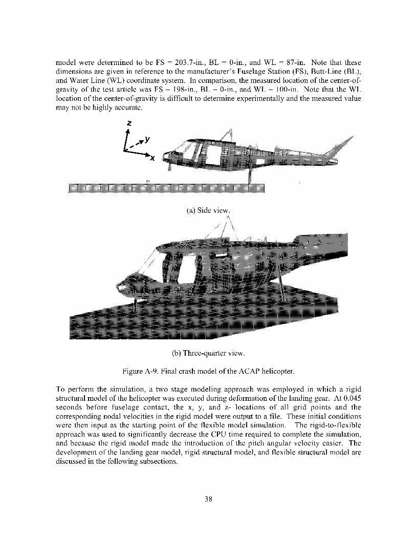
modelwere determinedto be FS= 203.7-in.,BL = 0-in., andWL = 87-in. Note that thesedimensionsaregivenin referenceto themanufacturer'sFuselageStation(FS),Butt-Line(BL),andWaterLine(WL) coordinatesystem.In comparison,themeasuredlocationof thecenter-of-gravityof thetestarticlewasFS= 198-in.,BL = 0-in., andWL = 100-in. Note thattheWLlocationof thecenter-of-gravityis difficult to determineexperimentallyandthemeasuredvaluemaynotbehighlyaccurate.

Z

(b) Three-quarter view.

Figure A-9. Final crash model of the ACAP helicopter.

To perform the simulation, a two stage modeling approach was employed in which a rigid

structural model of the helicopter was executed during deformation of the landing gear. At 0.045

seconds before fuselage contact, the x, y, and z- locations of all grid points and the

corresponding nodal velocities in the rigid model were output to a file. These initial conditions

were then input as the starting point of the flexible model simulation. The rigid-to-flexible

approach was used to significantly decrease the CPU time required to complete the simulation,

and because the rigid model made the introduction of the pitch angular velocity easier. The

development of the landing gear model, rigid structural model, and flexible structural model are

discussed in the following subsections.

38

A.2.1 Landing gear model

For impacts on hard surfaces, accurate simulation of the energy absorbing response of the

landing gear is imperative to accurately predict the impact response of the fuselage. The landing

gear stroking not only reduces the fuselage impact speed, but can also change the impact attitude.

The stroking of the landing gear, which can typically last 0.1 seconds, generally provides low

acceleration levels and primarily elastic deformations to the fuselage, as compared to the

fuselage impact event. These facts enabled utilization of a rigid fuselage model during most of

the landing gear stroking. The time step for a rigid model is typically an order of magnitude

larger than that for the flexible model, therefore the required clock time to perform a simulation

is reduced by an order of magnitude. For the model presented here, the CPU time was reduced

by a factor of eight. Additional details regarding the landing gear modeling can be found inReference 11.

A schematic of the ACAP main landing gear as viewed aft of the aircraft is shown in Figure A-

10. The main gear were designed with a two-stage, energy absorption approach. For landings

within the normal operational range, an oleo-pneumatic energy absorber was incorporated. For

severe or crash landings, additional energy is absorbed through stable crushing of an aluminum

honeycomb column within the gear. The transfer from the oleo-pneumatic to the honeycomb

stage is accomplished by shear pin failures based on a predetermined force. The orientation of

the gear with respect to the fuselage remains nearly constant while the oleo-pneumatic stage is

stroking. The initial angle with respect to the vertical, as shown in the figure, is 11.8 degrees.

As the honeycomb crushes, the gear rotates outward an additional 20 degrees. The drag beam

controls the gear rotation.

Vert__ _-'

Honeycomb t_

20.0o _/_,/ Fuselage attachments

Fuily_compressedf._,u_//_ v/

position "___,, ____ ..........

Oleo-pneumatic IJ'/_ _" ,

._, ,'/_ _ " urag oeam

Fully-extended _']¢_.j//'/./ \11.8 °

position "'--._ t___j[_ .....

Figure A-10. Schematic of ACAP landing gear looking aft.

To simplify the finite element model of the main landing gear mechanism as much as possible,

the angle of the landing gear was fixed with respect to the aircraft vertical axis. Therefore, the

39

translationalandrotationalmotionsof the gearhavebeenreplacedwith purely translationmotion. Theanglewasdeterminedby bisectingtheanglethroughwhichthe gearstrokes,or11.8° + 0.5x 20°= 21.8°, asshownin FigureA-10.

Initially, the landinggearmodelwasto be developedusinga numberof rigid joints, suchassliding,rotational,ball,anduniversaljointsthatarecurrentlyavailableasstandardcapabilitiesincommercialcodes.However,thesejoints maybecomeunstablewhenlargeforcesareapplied-suchasthoseexperiencedby thelandinggearduringa severeimpact. For this reason,thesebuilt-in joints werereplacedin themodelwith a componentcontaininga singlespringelementwith a user-definedforce responseto representboth the oleo-pneumaticand crushablehoneycombstages,andseveralbeamelementsthatwereusedto definethecorrectgeargeometryandto distributethe constraintforces,asshownin FigureA-11 (a). In general,the "spring"forceequationcanbedependenton therelativedisplacementandthe relativevelocity of theconnectednodes. This flexibility allowsauser-definedspringto simulatetheresponseof thevelocity dependentoleo-pneumaticstageandthe crushablehoneycombstage,which dependsonly ondisplacement.A FORTRANsubroutinewaswrittento simulatetheforceappliedto thefuselageby themain landinggearasthey stroke. Theequationsdefiningthe oleo-pneumaticportionarefoundin theKRASH85User'sGuide:AppendixA [12]. Theequationsaccountforthe air springfriction, hydraulic dampingand coulombfriction. Thevaluesfor the variousparametersdefiningtheACAPmainlandinggearweretakenfrom informationsuppliedby theairframemanufacturer.

Thetransitionfrom oleo-pneumaticto honeycombcrushingresultsfromtheshearpin failuresinthetestarticle. Becausetheoleo-pneumaticfriction forcesaredependenton thevelocity, anextremelylarge,shortdurationforceis appliedatthe initiation of contact.For thisreason,thesimulationwasnotableto usethecomputedforceto determinethetransition.As analternative,thedisplacement(stroke)of theoleo-pneumaticportionwasusedto triggerthetransition. Thecrushingof thehoneycombstageis representedby aconstantforceof 28,000lb. After fuselagecontact,theforcedueto thelandinggearisreducedto zeroasanapproximationof thetransferoftheloadfromthegearto thefuselagebelly.

Alignmentof the landinggearmodel relativeto the aircraftcanbe a challengingmodelingproblem. For this simulation,nodalalignmentwas accomplishedby creatingfour contactsurfacesontheoutersurfaceof twoperpendicularplates.Eachperpendicularplatewasmodeledwith arigid quadrilateralshellelement.Thenodesof thespringandbeamelementsformingthelanding gearmodel were then constrainedto remainwithin the intersectingregion of theperpendicularshells,asillustratedin FigureA-11 (b). Thethicknessof thealignmentshellswassetto providesufficientstabilitywithoutcreatingextremelylargecontactforces.Fortheresultspresentedin thispaper,theshellthicknesswas0.010in.

40

View A-A Fuselageattachment

Springelement

Beamelements

\

Tire

(a) Aft view, not to scale.

-- Beam elementswith associated

Alignment arex_ nodes

/_ ,!ii:iii_! i!lcklness

= 0.01 inch

surfaces (exaggerated)

(b) Vie,,,,, A-A, not to scale.

Figure A-11. Schematic of landing gear in the finite element model.

The original crashworthy nose gear was missing and had been replaced with a non-crashworthy

standard nose gem:. As described previously, modifications were required to make the existing

nose gear more crashworthy. The retrofitted nose gear was modeled as a spring having a

constant spring force of 8,000 lb. to represent the crush strength of the honeycomb-filled

aluminum tube that was inserted inside the gear.

A.2.2 Rigid structural model

A rigid structural model of the ACAP helicopter was created by changing all of the material

properties assigned to the elements to MATR]G, except for those elements forming the landing

gear. 214ATRIG is a specific material property card in MSC.Dytran that allows elements to be

defined as rigid bodies whose mass and moments of inertia are determined by the element

geometry and defined densiW. Once MAT"RIG is defined for an element, it cannot defbrm and

the code simply tracks the kinematic motion of the element as the simulation progresses. As

described in the previous section, landing gear forces were computed using an external

subromine. This procedure allowed quick runs to be made, of approximately one-hour duration,

to refine the con'elation of the sequence of events, and to ensure that the landing gear subroutine

accurately predicted the gear forces. For this model, it was important to ensure that the location

of the center-of-gravity and moments of inertia matched the experimental values closely. The

rigid model was executed for a duration of 0.045 seconds after left gear tire contact. The archive

files generated by the rigid model were post-processed in MSC.Patran with user-written

commands to create files containing nodal velocities and nodal positions at 0.045 seconds. The

nodal position file, which had the new GRID locations for each node, was input into the flexible

model using the INCI.UI)£ statement. The velocity file was read into the flexible model by anexternal user-written FORTRAN subroutine.

41

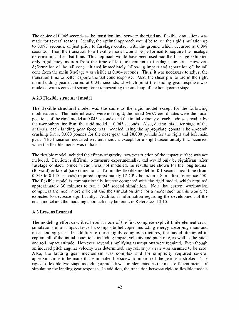
The choice of 0.045 seconds as the transition time between the rigid and flexible simulations was

made for several reasons. Ideally, the optimal approach would be to run the rigid simulation up

to 0.097 seconds, or just prior to fuselage contact with the ground which occurred at 0.098

seconds. Then the transition to a flexible model would be performed to capture the fuselage

deformations after that time. This approach would have been used had the fuselage exhibited

only rigid body motion from the time of left tire contact to fuselage contact. However,

deformation of the tail cone initiated immediately following impact and separation of the tail

cone from the main fuselage was visible at 0.064 seconds. Thus, it was necessary to adjust the

transition time to better capture the tail cone response. Also, the shear pin failure in the right

main landing gear occurred at 0.045 seconds, at which point the landing gear response was

modeled with a constant spring force representing the crushing of the honeycomb stage.

A.2.3 Flexible structural model

The flexible structural model was the same as the rigid model except for the following

modifications. The material cards were non-rigid, the initial GRID coordinates were the nodal

positions of the rigid model at 0.045 seconds, and the initial velocity of each node was read in by

the user subroutine from the rigid model at 0.045 seconds. Also, during this latter stage of the

analysis, each landing gear force was modeled using the appropriate constant honeycomb

crushing force, 8,000 pounds for the nose gear and 28,000 pounds for the right and left main

gear. The transition occurred without incident except for a slight discontinuity that occurredwhen the flexible model was initiated.

The flexible model included the effects of gravity, however friction of the impact surface was not

included. Friction is difficult to measure experimentally, and would only be significant after

fuselage contact. Since friction was not modeled, no results are shown for the longitudinal

(forward) or lateral (side) directions. To run the flexible model for 0.1 seconds real time (from

0.045 to 0.145 seconds) required approximately 12 CPU hours on a Sun Ultra Enterprise 450.

The flexible model is computationally intense compared with the rigid model, which required

approximately 30 minutes to run a .045 second simulation. Note that current workstation

computers are much more efficient and the simulation time for a model such as this would be

expected to decrease significantly. Additional information regarding the development of the

crash model and the modeling approach may be found in References 13-15.

A.3 Lessons Learned

The modeling effort described herein is one of the first complete explicit finite element crash

simulations of an impact test of a composite helicopter including energy absorbing main and

nose landing gear. In addition to these highly complex structures, the model attempted to

capture all of the initial conditions including impact velocity and pitch rate, as well as the pitch

and roll impact attitude. However, several simplifying assumptions were required. Even though

an induced pitch angular velocity was determined, any roll or yaw rate was assumed to be zero.

Also, the landing gear mechanism was complex and for simplicity required several

approximations to be made that eliminated the sideward motion of the gear as it stroked. The

rigid-to-flexible two-stage modeling approach was implemented as the most efficient means of

simulating the landing gear response. In addition, the transition between rigid to flexible models

42

causeda slight discontinuitythat occurredwhenthe flexible modelwas initiateddueto theinstantaneousonsetof the full landinggearhoneycombforce. Severaltechniquesto minimizediscontinuities(e.g., an accelerationspike at the transitionpoint from the rigid to flexiblemodels)were investigated,suchasrampingthe honeycombforce overmultiple time steps.However,noneof theseapproacheswascompletelyeffective.

Therigid-to-flexible two-stagemodelingapproach,alongwith the othersimplifications,didintroducesomeinaccuraciesinto themodel. Forexample,duringthecrashtest,thetail deformsandbeginsto fail soonafterthe landinggearforcesareappliedandbeforefuselagecontactwiththeground. However,in thecurrentmodelingapproach,thefuselagetail wasrepresentedasarigid bodyfor the first 0.045secondsof thesimulation. Consequently,thesimulationdid notpredictthe deformationof thetail from initial contactto 0.045seconds.Therigid-to-flexiblemodelingapproachwasusedbecauseit offeredan efficientmeansof introducingthe pitchangularvelocity. Anotherapproachto accountfortheangularvelocitywouldhavebeento writeanexternalsubroutineto calculatetheinitial x, y, andz componentsof velocityin theglobalaxissystemfor eachnodein themodel.

Whenfirst comparinganalyticalandexperimentaldata,it is oftendifficult to usetheraw, oreventhefiltered,accelerationresponsesto understandthephysicsof theimpactevent. In mostcases,it isbetterto examineandcomparethevelocityresponses.Kineticenergyis proportionalto velocitysquared,henceinaccuraciesin velocityarequiteimportant.Sincethehelicopterhada pitch rate aboutthe center-of-gravityinducedby the pendulum-swingtestmethod,eachlongitudinalpointonthehelicopterhadadifferentverticalandhorizontalcomponentof velocity.Any inaccuracyin the landinggearforces,landinggearmechanism,andin the landinggearandtire friction (whichwas ignored)duringthe rigid body phasecausesnot only the center-of-gravity velocity to be incorrect,but alsotherotationalvelocity aboutthe center-of-gravitytovaryincorrectly.

To illustratethevelocity comparisons,thepredictedandexperimentalvelocitiesat 0.045-and0.095-secondsandthepercentagedifferencebetweenthemareprovidedin TableA-1 for ninedifferent locationson the airframe. Thesetimeswere chosenfor their significancein thesimulationandin thetimesequenceof events.Thetimeof 0.045-secondswaschosenbecauseitis thetransitiontimebetweentherigid andflexiblesimulationsandthetimeof 0.095secondswas chosenbecauseit is just prior to fuselagecontactwith the ground. The percentagedifferenceslisted in TableA-1 were obtainedby subtractingthe experimentalvaluefrom theanalyticalvalue,thenthedifferencewasnormalizedby theexperimentalvalue. Thus,apositivepercentdifferencerepresentsanunderpredictionof thedata,while anegativevaluerepresentsanoverprediction.

Thevelocityresponsesfromtherigid simulationat0.045secondsagreeextremelywell with theexperimentalvalues,within +5%. However, by the time of fuselage contact, some deviations

have occurred, most notably for the right and left engine locations. Normally, one would

consider that these errors are a result of inaccuracies in the model; however, in this case, the

differences are due to electrical anomalies in the test data that adversely influenced the integrated

velocity responses. The floor-level velocity responses for the crew and troop seat locations and

at FS 182 agree well with the test data at both .045- and .095-seconds. The accuracy of the

43

predictedfloor-levelresponsesis moreimportantthanat otherlocations,sincethe floor-levelaccelerationpulseis transmittedthroughtheseatsto theoccupants.

TableA-1. Comparisonsof predictedandexperimentalvelocitiesfortime= 0.045-and0.095-secondsatninelocations.

Location Velocity(in/s)attime Velocity(in/s)attime== 0.045s 0.095s

Test Analysis % Diff Test Analysis %DiffPilot seatfloor -447.1 -456.4 -2.0 -483 -470.2 2.7Copilotseatfloor -444.4 -436.3 1.8 -452.6 -458.5 -1.3

-403.5 -382.5 5.2 -232.5 -181.3 22Toprt.maingearRightengine -362.6 -361.4 .3 -158.2 -209.4 -32.4*Left engine -353.8 -361.3 -2.1 -155 -201.4 -29.9*

-411.9-415.8 .9

.5-405.3

-312.3

-299.7Right troop floor

Left troop floor

-319.3

-311.4-403.2

-2.2

-3.9

Rotor head -393.6 -393.1 .1 -271.1 -262.3 3.2

Floor at FS 182 -412.3 -399.6 3.1 -311.4 -277.8 10.8

* Electrical anomalies in

responses.

the acceleration responses caused errors m the integrated test velocity

A similar comparison of predicted and experimental peak acceleration values was made for the

same nine locations as shown in Table A-2. Note that the experimental peak acceleration valueswere used to normalize the differences. The data shown in Table A-2 do not reflect differences

in phasing, i.e., time of occurrence of the peak acceleration values. Also, the data were obtained

from the plots of filtered analytical and experimental data. The same low-pass digital filter was

used for both sets of data. As shown in Table A-2, the predicted peak acceleration values of five

of the nine locations are within 20% of the experimental data. All of the predicted values are

within +40% of the experimental data with the exception of the rotor head location.

The large over prediction in the peak acceleration of the rotor head may be attributed to two

factors. First, a large number of vertical rod elements were used in the original modal-vibration

model. During the conversion of the modal-vibration model, all of the rod elements in the

subfloor were either removed or replaced with beam elements, since rod elements cannot bend

and are thus too stiff to represent the actual structural crash behavior. However, not all of the rod

elements in the upper fuselage were removed. Thus, the model of the upper fuselage had a

higher stiffness and exhibited less deformation than the actual structure, which contributed to the

over prediction of the peak acceleration. Another factor that may have contributed to the large

difference in peak acceleration at the rotor head location is the fact that the mass and inertia of

the troop seats and occupants were represented as concentrated masses that were attached to

nodes on the floor in the rear cabin area. However, the troop seats were mounted directly to the

ceiling, just under the rotor head location. A large downward deflection of the helicopter's roof

at the location of the wire-bender suspension system was observed in the high-speed film

coverage. Since the mass of the troop seats and occupants were not accurately located in the

model, this load path was not represented.

44

TableA-2. Comparisonsof predictedandexperimentalpeakaccelerationsatninelocations.

Location Peakacceleration,g

Pilot seatfloorTest90.1

Analysis115.6

%Diff-28.4

Copilotseatfloor 82.8 114.9 -38.8Rightmaingear(top) 33.8 33.2 1.6RightengineLeft engine

34.740.7

42.840.9

18.9.5

Righttroopfloor 75.4 63.6 15.751.7Left troopfloor

Rotorhead85.627.4 47.1

39.6-71.8

FlooratFS182 61.1 53.7 12.1

Theresultsin TableA-2 appearto raisequestionsregardingthe accuracyof the correlationbetweenthecrashsimulationpredictionsandthe testdata. However,severalfactorsmustbeconsideredin the evaluationof thisdata. Correlationbetweenanalyticalpredictionsgeneratedfrom a crashsimulationandtransientdynamictestdatais not straightforward.Dynamicdataobtainedfrom a full-scalecrashtestcontain,in general,highfrequencycomponentsthat oftenmaskthe underlying crashpulse. Also, the frequencyresponsesof the transducer,dataacquisitionsystem,andtheactualACAPhelicopterarenot thesameasthefrequencyresponseof themodel. Typically,thepredictedresponsescontainmorehigh amplitude,highfrequencyoscillationsthan the experimentaldata. In addition, sincethemodel is undamped,the highfrequenciesdonot decay.Consequently,eventhoughthesamelow-passdigital filter is appliedto boththeanalyticalandexperimentaldata,anequivalentlevelof filtering is notachievedsincethefrequencycontentandamplitudeof thefrequenciesof theanalyticalandexperimentaldataaredifferent.

In themodel,the seatsandoccupantswererepresentedusingconcentratedmasses.However,this approximationdoesnot accuratelyrepresentthe loading provided to the floor andsurroundingstructureby the actualenergyabsorbingseatsand occupants.Essentially,theapproachof modelingtheseatsandoccupantsasconcentratedmassesassumesthattheybehaveaslumpedmassesattacheddirectlyto the floor. In fact, the inertial loadingprovidedby theoccupantsis partiallydecoupledfrom the floor throughthe energyabsorbingseats.Theonlymeansof correctingthisdeficiencyin themodelis to physicallyrepresenttheseatsusingbeam,shell, and spring elementsand to simulatethe anthropomorphicdummiesusing a humanoccupantsimulationcodesuchasMADYMO [16] or ArticulatedTotalBody (ATB) [17]. Thisapproach,which is now possibledueto moreefficientcomputerresources,wouldhaveaddedconsiderablecomplexityto themodelandwasnotattempted.

Givenall of the factorsthat caninfluencethe testandanalysiscorrelation,it is obviouslyadifficult taskto quantifythe overallaccuracyof the crashsimulation.Theapproachdescribedhereinhasbeento presentthemodeldeformationsandthepredictedvelocity andaccelerationresponsesat severallocationsandcomparetheseresultswith testdata. In mostcases,thecrashsimulationpredictedthe overallshape,magnitude,anddurationof the experimentalresponsewell. Wherelargediscrepanciesoccurred,anattemptwasmadeto verify thetestdatafirst and

45

thento examinethemodelto understandtheanalyticalresults. Thesubjectof testandanalysiscorrelationhasbeenaddressedin two recentpublications,seeReferences18and 19. At thistime,othermethodsto assessthecorrelationaccuracybetweenanalyticaldatageneratedfrom adetailedfinite elementcrashsimulationandtransientdynamictestdataarebeinginvestigated.

A.4 References

1. Vaughan, V. L., Alfaro-Bou, E., "Impact Dynamics Research Facility for Full-Scale Aircraft

Crash Testing," NASA TN D-8179, April 1976.

2. Kay, B. F., and Maass, D., "Airframe Preliminary Design for an Advanced Composite

Airframe Program, Basic Report," Volume 1, Parts 1-3, USAAVRADCOM-TR-80-D-35A,March 1982.

3. Perschbacher, J.P., Clarke, C., Fumes, K., and Carnell, B., "Advanced Composite Airframe

Program (ACAP) Militarization Test and Evaluation (MT&E) Volume V- Airframe Drop Test,"

USAATCOM TR 88-D-22E, March 1996.

4. Thomson, D. T., and Clarke, C.W., "Advanced Composite Airframe Program (ACAP)

Militarization Test and Evaluation (MT&E) Volume I- Landing Gear Drop Test,"

USAAVSCOM TR-88-D-22A, August 1989.

5. Cronkhite, J. D., and Mazza, L. T., "Bell ACAP Full-Scale Aircraft Crash Test and KRASH

Correlation," Proceedings of the 44th Annual Forum of the American Helicopter Society,

Washington D.C., June 16-18, 1988.

6. Boitnott, R. L., Jones, L. E., "NASA Langley Research Center's Impact Dynamics Research

Facility Full-Scale Crash Test Procedures," Proceedings of the 3rd KRASH Users Seminar,

Arizona State University, Tempe, AZ, January 8-10, 2001.

7. Boitnott, R. L.; Jackson, K. E.; Fasanella, E. L.; Kellas, S.: "Full-Scale Crash Test of the

Sikorsky Advanced Composite Airframe Program Helicopter," Proceedings of the American

Helicopter Society Forum 56, Virginia Beach, VA, May 2-4, 2000.

8. Lahey, R. S., Miller, M. P., and Reymond, M., "MSC/NASTRAN Reference Manual, Version

68," The MacNeal-Schwendler Corporation, 1994.

9. Stebbins, R. F. and Twomey, W. J., "Plan, Formulate, and Discuss a NASTRAN Finite

Element Model of the Sikorsky ACAP Helicopter Airframe." NASA CR 182059, June 1990.

10. Anon., "MSC.PATRAN, DYTRAN Preference Guide," Publication No. 903077, Version 6,

The MacNeal-Schwendler Corporation, 1996.

11. Lyle, K. H., Jackson, K. E., and Fasanella, E. L., "Simulation of Aircraft Landing Gears with

a Nonlinear Transient Dynamic Finite Element Code," Journal of Aircraft, Vol. 39, No. 1,

January-February 2002.

46

12.Gamon,M.; Wittlin, G.;andLaBarge,B.: "KRASH85User'sGuide-Input/OutputFormat,"FinalReportDOT/FAA/CT-85/10,May 1985.

13.Lyle,K. H., Jackson,K.E.,Fasanella,E.L., "Developmentof anACAPHelicopterImpactModel,"Journal of the American Helicopter Society, Vol. 45, No. 2, April 2000, pp. 137-142.

14. Fasanella, E. L.; Jackson, K.E.; Lyle, K. H.: "Finite Element Simulation of a Full-Scale

Crash Test of a Composite Helicopter," accepted for publication in the Journal of the American

Helicopter Society, July 31,2001. Log Number 1128.

15. Fasanella, E. L.; Boitnott, R. L.; Lyle, K. H.; Jackson, K. E., "Full-Scale Crash Test and

Simulation of a Composite Helicopter," International Journal ofCrashworthiness, Vol. 6, No. 4,

November 2001, pp. 485-498.

16. MADYMO Users' Manual 3-D Version 4.3, the Dutch Institute of Applied Scientific

Research - Road/Vehicles Research Institute, Department of Injury Prevention, October 1988.

17. Obergefell, L. A., Gardner, T. R., Kaleps, I., and Fleck, J. T., "Articulated Total Body Model

Enhancements, Volume 2: User's Guide," AAMRL-TR-88-043, Harry G. Armstrong Aerospace

Medical Research Laboratory, Wright-Patterson Air Force Base, January 1988.

18. Lyle, K. H., Bark, L. W., Jackson, K. E., "Evaluation of Test/Analysis Correlation Methodsfor Crash Applications," Proceedings of the 57 th American Helicopter Society Annual Forum,

Washington D.C., May 9-11,2001.

19. Lyle, K. H., Bark, L., and Jackson, K. E., "Evaluation of Test/Analysis Correlation Methods

for Crash Applications," to be published in the Journal of the American Helicopter Society.

47

APPENDX B. B737 FUSELAGE SECTION CRASH SIMULATION

B.1 Experimental Program

B.I.1 Test set-up

A vertical drop test of a B737 fuselage section was conducted at the FAA Technical Center in

November of 2000 [1]. The test article is a 10-foot section of a Boeing 737-100 airplane from

fuselage stations (FS) 380 to 500. For this test, the fuselage section was outfitted with two

different overhead stowage bins. Also, 3,229-1bs. of luggage were packed in the cargo hold to

represent a maximum take-off weight condition. The objective of this test was to evaluate the

response of the overhead stowage bins in a narrow-body transport fuselage section when

subjected to a severe, but survivable, impact condition. In addition, this test provided an

invaluable opportunity to validate a nonlinear, explicit transient dynamic finite element crash

simulation of a transport aircraft. A pre-test photograph of the fuselage section is shown in

Figure B- 1.

The test article was outfitted with two commercial overhead stowage bins mounted in the

passenger cabin. A 60-inch Hitco bin was mounted on the left side of the cabin between FS 429

and FS 489. A 60-inch Heath Tecna bin was mounted on the right side of the cabin between FS

426 and FS 486. The overhead bins were loaded by installing 200-1bs. of plywood in the Hitco

bin and 120-1bs. of plywood in the Heath Tecna bin, corresponding to the maximum weights

specified for each bin. The bins were instrumented with five accelerometers. In addition, the

support linkages and brackets were heavily instrumented with strain gages that were calibrated to

provide axial load data.

Figure B-1. Pre-test photograph of the B727 fuselage section with overhead bins and luggage.

The passenger cabin was outfitted with 6 triple-occupant passenger seats and an instrumented

Hybrid II anthropomorphic dummy was placed in the center position of each seat, while the

remaining seats contained non-instrumented mannequins. The outer floor beams at each end of

48

thetestsectionwerereinforcedto minimizethe open-endeffects. Two largecameramounts,eachweighing70 lbs.,wereattachedto theupperfuselageframes.Twocameras,eachweighing22-1bs.,weresecuredto themountsto recordtheresponseof theoverheadbins. Thetotalweightof thefully instrumentedB737fuselagesectionwas8,870lbs.

Thefuselagesectionwasinstrumentedwith verticalandtri-axial accelerometersplacedon theinnerandouterseatrails andverticalaccelerometersmountedto theupperandlowerside-walls.Thesix anthropomorphicdummieswereinstrumentedwith pelvisaccelerometersandlumbarloadcells. In addition,theimpactplatformattheDynamicDropTestFacilitywasinstrumentedwith 12accelerometers,12loadcells,and12stringpotentiometerslocatedbeneaththeplatform.The fuselagesectionwas raisedto a heightof 14-ft.,andwasdroppedto achievea 30-ft/svertical velocity at impact. Approximately 140-channelsof datawere collectedat 10,000samples/secondduringtheimpacttestusingadigitaldataacquisitionsystem.

B.1.2 Summary of test results

A post-test photograph of the fuselage section is shown in Figure B-2. Structural damage

consisted of yielding and fracture of the lower fuselage frames and wrinkling of the skin on the

lower left side of the fuselage section. The deformation of the lower fuselage was asymmetric

about the centerline due to the presence of a cargo door and its associated stiffened structure

located on the lower right-hand side of the fuselage. On the left-hand side, a second damage site

developed with fracture of the fuselage frames. All seats on the right side of the fuselage floor

failed during the test. However, no failure of the overhead bin support brackets or linkages

occurred. Due to the presence of the luggage, the deformation pattern of the lower fuselage

frames was more uniform than typically seen in previous tests of transport fuselage sections [2].

Figure B-2. Post-test photograph of the B737 fuselage section with bins and luggage.

The cargo door introduces asymmetry into the fuselage configuration including asymmetry about

the centerline since the door is only on the right side of the cargo area, and asymmetry about the

mid-plane since the door is located closer to the rear of the section than to the front. To

determine the influence of the door, the acceleration traces obtained from two accelerometers

located on the right and left outer seat tracks at FS 418 were integrated to obtain the velocity

49

timehistoriesshownin FigureB-3. Thisplot indicatesthatuntil about0.06seconds,thetworesponsesarenearlythesame.After thattime,thevelocityon theright sideis beingremovedsomewhatmorequickly thanon theleft side,asaresultof the stiff cargodoorlocatedon theright sideof the lower fuselage.Thevelocity responsesof the right andleft outerseattracklocationshavecrossedzerovelocityby0.11and0.12seconds,respectively.

lO

o

-lO

-20

-30

-40

Velocity, ft/s30

20 .......[__-___.RightLeftsidesidefloor,floor'FsFS418418]|...........

..........................i..........................i>'P:"i i'"

i ,a.# i

i m i

i ,_,° i

,," i i .....................

i i i ill i i ill i i iii i i i ill i i i i i i i

0 0.05 0.1 0.15

Time, s

Figure B-3. Floor-level velocity versus time responses.

B.2 Description of the Modeling Approach

The model geometry was developed from detailed geometric measurements made of the test

article, since engineering or technical drawings of the fuselage section were not available.

Several assumptions were made to keep the geometry as simple as possible. For example, many

of the cutouts, joints, fasteners, and doublers were ignored. Development of the model was

performed using the pre-processing software package, MSC.Patran [3]. A geometric model of

the fuselage section, shown in Figure B-4, was developed containing the important structural

features of the airframe. The geometric model was discretized, and element and material

properties were assigned. The complete finite element model of the B737 fuselage section with

the overhead bins and luggage is shown in Figure B-5.

The MSC.Dytran [4] model contains 9,759 nodes and 13,638 elements, including 9,322 shell and

4,316 beam elements, and 250 concentrated masses to represent the outer skin, fuselage frames,

floor, longitudinal stringers, the fore and aft floor reinforcements, the camera mounts, and the

overhead bins. In addition, the cargo door on the lower right side of the fuselage section was

modeled, including its associated stiffened structure. Cutouts in the fuselage skin were used to

represent the windows on both sides of the section and the stiffened structure surrounding the

windows was modeled using beam elements. A flat impact surface was added to the model.

Each edge node on the impact surface was fixed; i.e. the nodes were constrained from

translational and rotational motion. Some of the individual components of the model are shown

in Figure B-6, including the outer skin, fuselage frames, floor, floor beams, stringers and door.

50

Note thatthebeamelementsaredifficult to distinguishfromthe shellelementsin thefigureastheyarerepresentedasstraightlines.

:_................. ,_.............. ,_.............. _i..,_i

(a) Front view.

iiiii¸

iiiii¸

iiiiiiiii: iiiiii

iiiiii

(c) Geometry model with surfaces.

Figure B-4. Geometry model of the B737 fuselage section.

A master-surface to slave-node contact was defined between the impact surface and the nodes

forming the lower portion of the fuselage section. This contact definition prevents the structural

model from passing through the impact surface. Two additional contact surfaces were defined

between the fuselage structure and the Heath Tecna and Hitco bins. These contact surfaces were

defined to prevent the bins from passing through the fuselage during impact.

51

HeathTecnabin

Cameramounts

Hitcobin

Rightside Left side

Impactsurface

FigureB-5.FiniteelementmodeloftheB737fuselagesection(frontview).

iiiii_i_ iiiii

(a) Outer skin. (b) Frames and floor beams.

(c) Door and stringer beams. (d) Floor and floor beams.

Figure B-6. Components of the MSC.Dytran model of the B737 fuselage section.

The seats and dummies were not modeled physically; however, the mass of the seats and

dummies was combined and accounted for as 24 concentrated masses that were assigned to

52

nodeslocatedateachseatleg-seattrackpositionon thefloor. Otherconcentratedmasseswereusedto representthe plywood in eachoverheadbin, the camerassupportedby the cameramounts,andthe luggage. As describedpreviously,3,229-1bs.of luggagewereplacedin thecargohold beneaththefloor of the fuselagesectionprior to the impacttest. Theluggagewastightly packedandsecuredusingstrapsandnetting. Severaltechniqueswereusedto representtheinertialpropertiesof theluggagein thefiniteelementmodel. Thefinal approachwasto usea"percentageareamethod."A linewasdrawnhorizontallyattheexpectedheightof the luggage,whichwasapproximately1-ft.belowthefloor. Thetotalareaencompassedbelowthehorizontalline andtheinnerfuselageframeswascalculated.Next,linesweredrawnvertically from eachnodein theregion to intersectthe horizontalline. The percentageareaof each"rectangle"formedwasdeterminedby dividingthesmallareaof eachindividualrectangleby thetotal area.Theseratioswere thenusedto determinethe percentageof the 3,229-1bs.of luggageto beassignedto thenodesatthatlocation.Usingthisapproach,60%of theweightof the luggage,or1,937lbs.,wasattachedto thenodesformingthecargofloor. Theremainingweightof 1,292-lbs.wasappliedin decreasingamountsto thenodesalongbothsidesof thefuselageframes.Itwasassumedthatthefuselagesectionwasloadeduniformlyfrom frontto backbytheluggage.

Thismethodof modelingtheluggagewasselectedbecauseit is efficientandit representsafairlyaccuratedistributionof the loadingprovidedby the luggageto the fuselageframesat initialimpact. However,severalimportantpropertiesof theactualluggagearenotmodeledusingthisapproach.Forexample,theinertiaof the luggageis approximatedandis distributedto thenodeson the fuselageframes. Duringthe impact,theweightof the luggagecanshift andprovideadifferent loadingpath to the fuselagestructure,which cannotbe modeledusingthe currentapproach.Thefrictionalcontactbetweenthefuselagesectionandtheluggageis notmodeled.Sincethe individualpiecesof luggagearenotmodeled,no materialpropertiesareassignedtorepresentthe"compressibility"of the luggage.Duringtheactualimpact,the luggagewill reacttheloadsappliedby thefuselagefloor andthelowerfuselageframesandskin. However,sincetheluggageis notphysicallymodeled,thereisnomechanismto developandapplythesereactiveforces. Oneobviousway to correctthesedeficienciesin themodelis to representthe luggageusingsolidelementsandto assignamaterialpropertythataccuratelyrepresentsthecompressivepropertiesof the luggage.However,thisapproachwasnot takeninitially dueto thefactthatnodataonthematerialpropertiesof luggagewereavailable.

Most of theprimary structurewasassumedto be either2024-T3or 7075-T6aluminum.Thematerialformulationchosenfor the model,DMATEP, is a general-purposeisotropicbilinearelastic-plasticmaterialpropertywith yielding,strainhardening,andultimatefailurestrain. Theyield stressof 2024-T3wasassumedto be47,000psi,while the yield stressof 7075-T6wasassumedto be 60,000psi. The yield stressof the 7075-T6aluminumwas lowered fromhandbookvalues(73,000psi) to partiallyaccountfor stressrisers,fatiguedamage,sizeeffects,andcorrosion. Initially, themodelwasexecutedwithout failure. Later,a failure strainof 5percentwasassignedto the 7075-T6aluminumbasedon experiencegainedduringanearlierprojectinvolving simulationof a Boeing720fuselagesectiondroptest [2]. A list of materialpropertiesusedin themodelisprovidedinTableB-1.

A photographof theHeathTecnabin installedin thefuselagesectionis shownin FigureB-7(a).Thebin is locatedon theright or doorsideof thefuselagesection.Thebin weighs56 lbs.and

53

consistsof afiberglassshellanda compositesandwichfloor. Thebin is securedto theaircraftby instrumentedsupportbracketsand cylindrical struts, including C- and L-cross-sectionmountingrails attachedto the fuselageframes. Two vertically-mountedstrutsand matingsupports,designatedHT-1,HT-2,HT-3,andHT-4 in FigureB-7(b),areusedto attachthebintotheceilingof thetestsectionandto providesupportfor verticalloading. Theverticalstrutsare0.5-inchdiametersolidcylindricalrods,approximately14-inchesin length. Forthedroptest,thebinwasloadedwith 120-1bs.of plywood.

TableB-1.Materialpropertiesusedin theMSC.Dytranmodelof theB737fuselagesectionwithoverheadbinsandluggage.

Materialname Material Young's Density, Poisson's Yieldtype modulus, lb-sZ/in4 ratio stress,

psi psiAluminum2024-T3 DMATEP 1.06e07 .0002525 .33 47,000Aluminum7075-T6 DMATEP 1.04e07 .0002525 .33 60,000HeathTecnaverticalstruts DMATEP 1.04e07 .0002525 .33 N/AHeathTecnaoutershell DMATEP 2.75e06 .0000638 .35 N/AHeathTecnafloor DMATEP 5.0e06 .0001146 .35 N/AHitcooutershell DMATEP 2.75e06 .00012 .33 N/AHitcobin floor DMATEP 2.75e06 .0001137 .33 N/A

Hitco linkages DMATEP 1.04e07 .0002525 .33 N/A

Impactsurface DMATEP 9.0e08 0.00075 0.3 N/A

Thefinite elementmodelof theHeathTecnabin is shownin FigureB-8. Theoutersurfacesandfloor of thebin aremodeledusingshellelements.Theverticalstrutsthat attachthebin floor totheC-mountingrails aremodeledusingone-dimensionalbeamelements.Beamelementscancarryaxial load,aswell asbending,torsional,andshearloads. In thetestarticle,thestrutsareinclinedat anangleof approximately5° from true vertical. The elementsrepresentingthesestrutsareinclinedatthesameanglein themodel.

The C-mountingrails aremodeledusing shell elements. In the test article, the C-railsareattachedto thefuselageframesusingbrackets.In themodel,theC-railsareattachedusingbeamelements.Thebin floor is alsosecuredto thefuselagesectionthroughanL-mountingrail thatisattachedto thefuselageframesat five locations,asshownin FiguresB-7 andB-8. Thebin isattachedto theL-mountingrail attwo locationsby brackets.In themodel,theL-mountingrailandbracketsaremodeledusingshellelements.Theplywoodthatwasplacedin theHeathTecnabin is modeledas15concentratedmasses,eachweighing8 lbs. Thesemassesareattachedtonodesonthebin floorandareuniformlyspacedalongthelengthandwidth of theplatform.

Threeuniquematerialpropertieswereassignedto theelementsformingtheoutersurfaceof thebin,thebin floor,andtheverticalstruts.Thedensitiesof thematerialsassignedto theoutershellandbin floor wereadjustedsuchthatthetotalemptyweightof theHeathTecnabin was56 lbs.A third materialpropertywasassignedto the elementsrepresentingthe vertical struts. Thespecificmaterialpropertiesusedin themodelarelisted in TableB-1. Note that thematerial

54

propertiesof the outershellandfloor of the HeathTecnabin areunknownandthatthevaluesassignedto themareestimatesbasedonengineeringjudgment.Until thesepropertiesareknownandinputinto themodel,it is notpossibleto determineaccuratelytheeffectivestressor straininthe bin as a function of time. The doorlatch of the bin is not modeled,sincethis bin wasstrappedshutpriorto theimpacttest.

(a)Photographof theHeathTecnabininstalledin theB737fuselagesection.

i iii̧

i!:ii

_i_ii!_i_!_ _

/ I_: ..............................;

}i i_iiii_iil

(b) Component designations for the Heath Tecna overhead bin.

Figure B-7. Heath Tecna bin photograph and component designations.

Following inspection of the Heath Tecna bin, it was determined that the components most

critical for maintaining structural integrity during impact were the vertical support struts and

mating brackets. The FAA supplied one of the 0.5-in. diameter struts and its mating bracket for

testing. The strut is notched on one end and is attached to the bracket by a through bolt, while

the other end is threaded. An 0.25-in. diameter eyebolt is screwed into the strut and is attached

to a triangular bracket on the loading platform with a single 0.25-in. diameter bolt and lock nut.

A tensile test was performed on the Heath Tecna vertical strut and bracket assembly. The

notched end of the strut was loaded through the bracket and the threaded end was loaded through

55

theeyebolt.To ensurethatonlytensileloadswereapplied,atestfixturewasfabricatedto alignthebracketwith theeyebolt. Thestrutwasloadedquasi-staticallyusingabench-toploadtestmachine.Themeasuredload-deflectioncurveis shownin FigureB-9 (a). Theassemblyfailedattheholewherethebolt connectsthenotchedendof thestrutto thebracket,asshownin FigureB-9(b). Themeasuredultimatefailureloadwas1,656lbs. Thistestresultprovidesasingledatapoint that canbeusedasa guidelinefor evaluatingfailure of the strutandmating bracket.However,it mustbenotedthatthe actualcomponentsmayexperienceamuchmorecomplexloadingscenario,includingshear,bending,andtorsionduringtheimpacttest. In themodel,theverticalsupportstrutswereassignedmaterialpropertiestypical of 7075-T6aluminumwith noyieldingor failure. Theaxialforceresponsesof thebeamelementsrepresentingthestrutswereoutputfor correlationwith thecalibratedloaddataobtainedfromthestraingages.

HT-5

HZ-q

HT-9

............................... HT-3 .....

(a) Three-quarter view. (b) Front view.

HT-1

(c) Side view.

Figure B-8. Finite element model of the Heath Tecna bin.

A photograph of the Hitco overhead bin is shown in Figure B-10 (a) prior to installation. This

bin is located on the left side of the fuselage section and consists of an outer shell, floor, and

several support linkages. The empty bin weighs 57 lbs. For the test, the bin was loaded with

200-1bs. of plywood and instrumented with five accelerometers. The bin is secured to the

airframe by 11 support linkages, as shown in Figure B-10 (b), which were instrumented with

strain gages for the test. Vertical support is provided by two 1.5-in. diameter links that are

attached to the fuselage frames at FS 400 and FS 420 and at FS 460 and FS 480. These links are

attached to the overhead bin through two 0.616-in. diameter tie-rod links that are approximately

56

10inchesin lengthandarethreadedon oneendto receivea 0.25-in.diametereye-screw.Theeye-screwsareattachedto bracketslocatedonboth endsof the bin with a bolt andlock nut.Whenthebin is mountedto thefuselagesection,the0.616-in.diametertie-rodlinks areorientedvertically.

In addition,thebinis supportedbytwo 1.25-in.diameterlinksthatareattachedatFS400andFS420andat FS460 andFS480usingtwo 0.437-in.diametersupportlinks at eachframe. The1.25-in.diameterlinks areattachedto therearof thebin throughbrackets.Finally, a0.56-in.diameterstrutlink wasattachedfromtheendof the1.25-in.-diameterlink to thefuselageframelocatedat FS440to providelongitudinalsupportfor thebin. TheFAA performedtensiletestson the 0.437-in.and0.616-in.diameterlinks in whichultimatefailure loadsof approximately4,000-and5,000-1bs.wereobtained,respectively.Theseloadscanbeusedasguidelinesforevaluatingfailureof thelinkages.

...." "_i}i.............i.............. _ _ Failure load

i :i S _::i 1,656 lbs.

ii i iii iii ; i

i , i,, ::i/ i :: i ' % i

(a) Load versus displacement response.

Bracketfailure

(b) Photograph showing failed bracket.

Figure B-9. Load versus displacement response of a Heath Tecna vertical support strut assembly.

The finite element model of the Hitco bin is shown in Figure B-11. The outer surfaces and floor

of the bin are modeled using shell elements and the support linkages are modeled using beam

elements. A wall thickness of 0.125-inches was specified for each of the tubular support links.

The mass and inertial properties of the 200-1bs of plywood added to the Hitco bin are represented

as 24 concentrated masses, each weighing 8.33-1bs. These masses are attached to nodes on the

bin floor and are uniformly spaced along the length and width of the platform. Three different

material properties were defined for the elements forming the Hitco bin. The densities of the

materials assigned to the outer shell and floor were adjusted such that the total weight of the

empty bin is 57 lbs. The support linkages were assigned material properties typical of 7075-T6

aluminum with no yielding or failure, and the axial force response was requested as output. The

specific material properties are listed in Table B-1. As with the Heath Tecna bin, the material

properties of the outer shell and floor of the Hitco bin are unknown and the values assigned to

them are estimates based on engineering judgment. Until these properties are known and input

into the model, it is not possible to determine accurately the effective stress or strain in the bin as

a function of time. Also, it is important to note that the door latch of the bin is not modeled,

since this bin was strapped shut prior to the impact test.

57

(a)Photographof theHitcooverheadstowagebin andsupportlinkages.-_Z_........ _''''"_

ili

i,i:_ii!i

(b) Component designations for the Hitco bin.

Figure B-10. Photograph and component designations for the Hitco bin.iliiii

(a) Three-quarter view. (b) Front view.

................:lli:i. ........................ _${. "..............:...........................ii{ ...............

(c) Side view.

Figure B-11. Finite element model of the Hitco bin.

One check of the integrity of the finite element model is to compare the mass of the individual

components with the corresponding weights of the test article. A weight comparison of the test

article and model is shown in Table B-2. The total weight of the model is 4.5% heavier than the

actual B737 fuselage section. The differences in mass appear in the empty weight of the

fuselage section and in the combined seat, occupant, and other weights that are accounted for in

58

the model using concentratedmasses. The emptyweight of the model is expectedto besomewhatheavierthat the actualfuselagedueto the fact that most of the cutoutswerenotincluded.Also,averagethicknesseswereusedin themodel,whereasthegeometryof theactualfuselagesectionvariedgreatlyfrom locationto location. Thetotalweightof all concentratedmassesis somewhathigherthantheexperimentalvaluedueto thefactthatmanysmallmasses(2-3 lbs.each)wereassignedto nodeswhereoutputwasrequestedasameansof loweringthehigh-frequencyresponse.

Anothercheckof themodelis to comparethelocationsof thecenter-of-gravityfor thetestarticleandthemodel. Thecenter-of-gravityof thefinite elementmodelis locatedatx = 60.9,y = -4.2,andz = 62.4inches,wherex is the longitudinaldirection,y is the lateraldirection,andz is thevertical direction. This location is slightly forward of the mid-plane,slightly left of thecenterline,andapproximately1inch abovethefloor. Thus,thecenter-of-gravitylocationof themodelreflectstheasymmetrycausedby the cargodoor. Thecenter-of-gravitylocationof thetestarticlewasnotdeterminedexperimentally.

TableB-2.Weightcomparisonof themodelandtestarticle.

Component Testweight,lbs. Modelweight,lbs.

Fuselagesection,empty 1,360 1,526

Combinedseats,occupants,&misc. 3,620 3,845Hitcobin andwoodmass 257 257HeathTecnabin andmass 176 176Camerasandmount 228 240Luggage 3,229 3,230Total 8,870 9,274

It is importantto understandfully theassumptionsandapproximationsmadein developingandexecutingthemodel. For example,sinceengineeringdrawingswerenot available,the grossgeometryof the sectionwas determinedthroughmeasurementsmadeby hand usingtapemeasuresand digital calipers. The level of accuracyof the analytical and experimentalcorrelationwill determine,in somerespects,whethertheapproximationsusedwerevalid. Theassumptionsandapproximationsmadein developmentof themodelarelisted,asfollows:

• It is assumedthattheimpactoccurswithno roll, pitch,oryaw.• The impact condition is assumedto be 30-ft/s vertical velocity, with no lateral,

longitudinal,or rotationalvelocitycomponents.• ThewoodenimpactplatformattheDynamicDropTestFacilityattheFAA is assumedto

behaveasarigid surface.• The geometryof the outerfuselageskin, frames,stringers,floor, andotherfeaturesis

approximatedasuniformalongthelengthof thefuselagesection.Inconsistenciesin thegeometrywere averaged. For example,a largevariation in the skin thicknesswasmeasuredaroundthe circumferenceof the fuselage. Insteadof incorporatingthesevariationsin themodel,anaveragevaluewasdeterminedandused.

• Thematerialpropertiesassignedto the elementsrepresentingthe fuselagesectionareestimated.Basedoncorrosion,stressconcentrations,fatiguedamage,andamultitudeof

59

otherfactors,thenumbersusedfor yield stressandultimatefailurestrainmaybereducedby anorderof magnitudefrom the original materialproperties,or valuesobtainedinengineeringhandbooks.No testswereperformedoncomponentsfrom the fuselagetodeterminetheactualmaterialproperties.Thus,thevaluesusedin themodelarebasedonengineeringjudgment,pastexperience,andmaterialhandbookdata.

• Many of the cutouts,fittings, attachments,doublers,andjoints arenot includedin themodel. For example,noneof therivetswereincluded. Thecutoutswereaccountedforby decreasingtheaveragethicknessof thespecificcomponent.Somelargecutouts,e.g.thewindows,wereincludedin themodel.

• The seats,occupants,and other weights on the floor are assumedto behaveasconcentratedmassesattachedto nodesattheir approximatelocationin themodel. Theinertialpropertiesof thecomponentsareapproximated.

• Wherepossible,thecomponentsof thefuselagesectionaremodeledusingshellelementssincetheseelementsareextremelyefficientin MSC.Dytran.However,beamelementswere usedto representthe stringers,door andwindow frames,andother reinforcingstructure.

• Theluggageis modeledusingconcentratedmasseslocatedonnodesformingthelowerfuselageframes. This approximationof the luggagewasmadefor efficiency of thesimulationandbecausematerialpropertydatafor luggagewerenotavailable.However,as discussedpreviously, this non-geometric,non-physical representationcannotaccuratelysimulatethebehaviorof theluggageduringthetest.

• TheHeathTecnaandHitco supportlinkagesaremodeledusingone-dimensionalbeamelements,insteadof rod elements.Beamelementscansupportaxial,bending,andshearloads,whereasrodelementscanonly reactaxialloads. Thedecisionto usebeamversusrod elementswasmadeto reflectthefact thatthesupportlinkagesareconstrainedsuchthat they areprimarily loadedin the axial direction. However,it is possiblethat thesupportlinksmayexperienceamorecomplexloadingscenario.

• It is assumedthatthedoorlatcheson theHeathTecnaandHitcobinscannotbeopened.Consequently,theywerenot includedin themodelsofthebins.

Themodelwasexecutedin MSC.Dytran[4] for 0.2secondsof simulationtime ona SunUltraEnterprise450 workstationcomputer.The simulationrequired36hoursof CPUwith a finaltime stepof 2.67microseconds. Requestedoutput included the deformedgeometryandacceleration,velocity, and displacementtime histories for severalnodeswhosepositionscorrespondto thelocationsof selectedtransducers.

B.3 Lessons Learned

A comparison of the predicted and experimental peak acceleration values for the right and left

inner and outer seat track locations is shown in Table B-3. In general, the predicted seat track

acceleration responses matched the overall shape and duration of the experimental acceleration

pulses fairly well and the experimental peak acceleration values were well predicted i.e., within

approximately 25% except for the left inner seat rail at FS 418 and FS 452. In general, the

degree of correlation was surprising given the large number of approximations used in the model

development. One suggestion that would result in a more accurate representation of the test

60

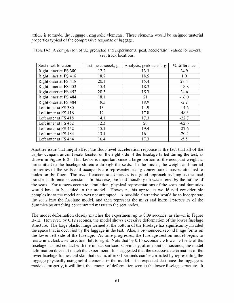
articleis to modelthe luggageusingsolidelements.Theseelementswouldbeassignedmaterialpropertiestypicalof thecompressiveresponseof luggage.

TableB-3.A comparisonof thepredictedandexperimentalpeakaccelerationvaluesfor severalseattracklocations.

Seattracklocation Test,peakaccel.,g Analysis,peakaccel.,g %differenceRightinneratFS380 17.7 13.3 24.9RightinneratFS418 18.7 18.5 1.0RightouteratFS418 20.1 15.4 23.4RightinneratFS452 15.4 18.3 -18.8RightouteratFS452 20.3 15.3 24.6RightinneratFS484 18.1 21 -16.0RightouteratFS484 18.5 18.9 -2.2Left inneratFS380 13 14.9 -14.6Left inneratFS418 12 17.8 -48.3Left outeratFS418 14.1 17.3 -22.7Left inneratFS452 12.3 20 -62.6Left outeratFS452 15.2 19.4 -27.6Left inneratFS484 13.4 16.1 -20.2Left outeratFS484 16.4 17.3 -5.5

Anotherissuethatmight affectthe floor-level accelerationresponseis the fact that all of thetriple-occupantaircraftseatslocatedon theright sideof thefuselagefailed duringthetest,asshownin FigureB-2. This factoris importantsincea largeportionof theoccupantweight istransmittedto the fuselagestructurethroughthe seats. In the model,the weightandinertialpropertiesof the seatsand occupantsarerepresentedusingconcentratedmassesattachedtonodeson the floor. Theuseof concentratedmassesis a goodapproachaslong asthe loadtransferpathremainsconstant.In this case,the loadtransferpathwasalteredby thefailureoftheseats. For a moreaccuratesimulation,physicalrepresentationsof theseatsanddummieswould have to be addedto the model. However, this approachwould add considerablecomplexityto themodelandwasnot attempted.A possiblealternativewouldbeto incorporatethe seatsinto the fuselagemodel, andthen representthe massandinertial propertiesof thedummiesby attachingconcentratedmassesto theseatnodes.

Themodeldeformationcloselymatchestheexperimentup to 0.09seconds,asshownin FigureB-12. However,by 0.12seconds,themodelshowsexcessivedeformationof thelower fuselagestructure.Thelargeplastichingeformedatthebottomof thefuselagehassignificantlyinvadedthespacethatis occupiedby theluggagein thetest. Also,apronouncedsecondhingeformsonthelower left sideof the fuselage.As time progresses,the fuselagesectionmodelbeginstorotatein aclockwisedirection,left to right. Notethatby 0.15secondsthelower left sideof thefuselagehaslostcontactwith the impactsurface.Obviously,afterabout0.1seconds,themodeldeformationdoesnotmatchtheexperiment.It is suggestedthattheexcessivedeformationof thelowerfuselageframesandskinthatoccursafter0.1secondscanbecorrectedbyrepresentingtheluggagephysicallyusingsolid elementsin themodel. It is expectedthat oncethe luggageismodeledproperly,it will limit theamountof deformationseenin the lowerfuselagestructure.It

61

is alsopossiblethatthematerialpropertiesassignedto theelementsformingthelower fuselagestructurearenot correct. Sinceno materialstestingwasperformed,the propertiesusedwereestimatedbasedonengineeringjudgment.Consequently,variationsin Young'smodulus,yieldstress,strain-hardeningmodulus,andultimatefailurestrainshouldbe investigated,aswell.

Pre-testmodel

ii:: f

t = 0.03 seconds

t = 0.06 seconds

t = 0.09 seconds

t = 0.12 seconds

iiii!it!ii!!iii iiii Iiiiiii

Experiment

t = 0.03 seconds

t = 0.06 seconds

t = 0.09 seconds

t = 0.12 seconds

t = 0.15 seconds t = 0.15 seconds

Figure B-12. Comparison of predicted deformation with photographs form the high-speed film.

62

By .06seconds,a seconddamagesiteon thelowerright sideof thefuselagesectionhasdeveloped.Thissecondarydamagesite is notpredictedby themodel. Instead,thecargodoorareaon thelower right sideof the fuselagemodelremainsintactwith no signof bucklingorfailure. Theseresultsindicatethatthemodelof thecargodoordoesnothavesufficientfidelityto capturetheobservedfailure. A suggestedmodelimprovementis to re-examinethecargodoormodelandto makeadjustmentsasnecessaryto obtaina better representationof the actualstructure.More information on the developmentof the B737 fuselagesectionmodel andsimulationcorrelationcanbefoundin References5 and6.

B.4 References

1. Abramowitz, A., Smith, T. G., Vu, T., Zvanya, J. R., "Vertical Drop Test of a Narrow-Body

Transport Fuselage Section with Overhead Stowage Bins Onboard," DOT/FAA/AR-01/100, to

be published.

2. Fasanella, E. L., Widmayer, E., and Robinson, M.P., "Structural Analysis of the Controlled

Impact Demonstration of a Jet Transport Airplane," Journal of Aircraft, Volume 24, April 1987,

pp. 274-280.

3. MSC.Patran Users Manual, Version 2000, MSC.Software Corporation, Los Angeles, CA,1999.

4. MSC.Dytran User's Manual Version 4.7, The MSC-Software Corporation, Los Angeles, CA,1999.

5. Jackson, K. E. and Fasanella, E. L., "Crash Simulation of a Vertical Drop Test of a B737

Fuselage Section with Overhead Bins and Luggage," Proceedings of the Third Triennial Aircraft

Fire and Cabin Safety Conference, Atlantic City, NJ, October 22-25,2001.

6. Fasanella, E. L. and Jackson, K. E., "Crash Simulation of a Vertical Drop Test of a B737

Fuselage Section with an Auxiliary Fuel Tank," Proceedings of the Third Triennial Aircraft Fire

and Cabin Safety Conference, Atlantic City, N J, October 22-25,2001.

63

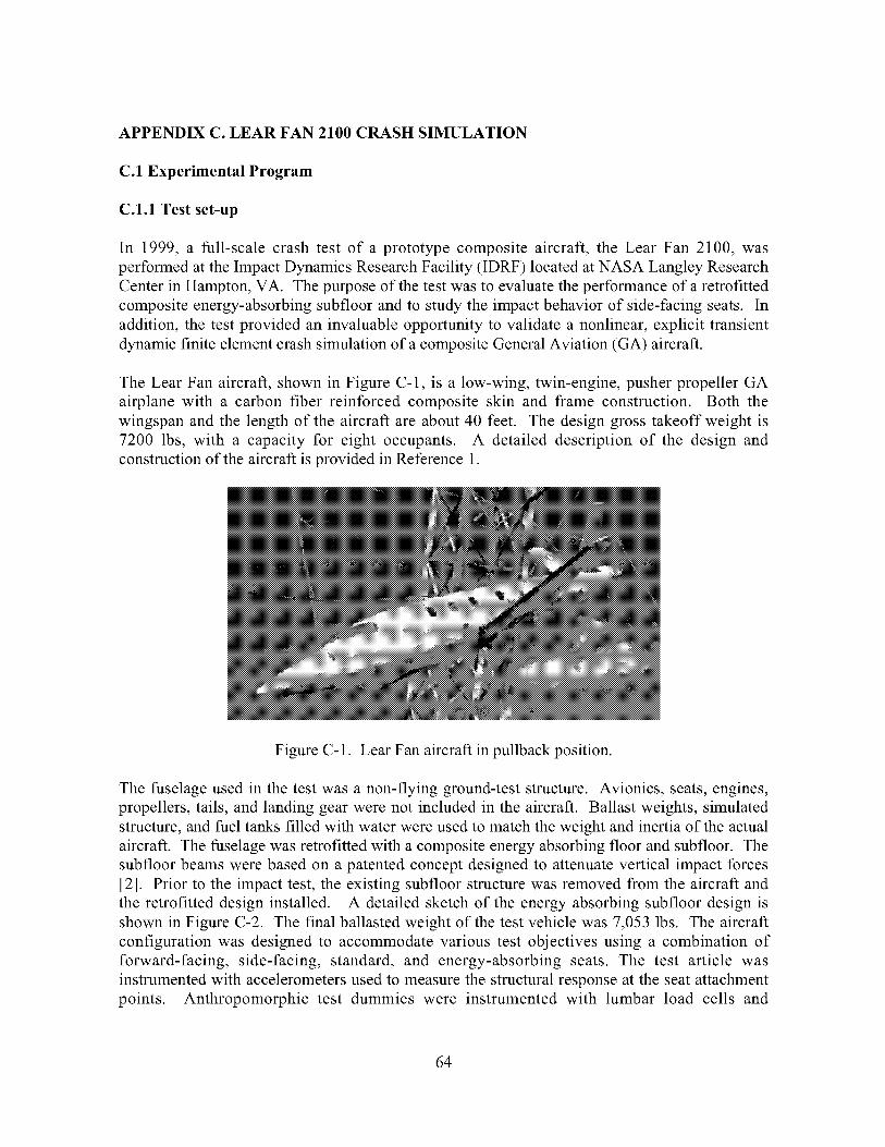
APPENDIX C. LEAR FAN 2100 CRASH SIMULATION

C.1 Experimental Program

C.I.1 Test set-up

In 1999, a full-scale crash test of a prototype composite aircraft, the Lear Fan 2100, was

performed at the Impact Dynamics Research Facility (IDRF) located at NASA Langley Research

Center in Hampton, VA. The purpose of the test was to evaluate the performance of a retrofitted

composite energy-absorbing subfloor and to study the impact behavior of side-facing seats. In

addition, the test provided an invaluable opportunity to validate a nonlinear, explicit transient

dynamic finite element crash simulation of a composite General Aviation (GA) aircraft.

The Lear Fan aircraft, shown in Figure C-l, is a low-wing, twin-engine, pusher propeller GA

airplane with a carbon fiber reinforced composite skin and frame construction. Both the

wingspan and the length of the aircraft are about 40 feet. The design gross takeoff weight is

7200 lbs, with a capacity for eight occupants. A detailed description of the design and

construction of the aircraft is provided in Reference 1.

Figure C-1. Lear Fan aircraft in pullback position.

The fuselage used in the test was a non-flying ground-test structure. Avionics, seats, engines,

propellers, tails, and landing gear were not included in the aircraft. Ballast weights, simulated

structure, and fuel tanks filled with water were used to match the weight and inertia of the actual

aircraft. The fuselage was retrofitted with a composite energy absorbing floor and subfloor. The

subfloor beams were based on a patented concept designed to attenuate vertical impact forces

[2]. Prior to the impact test, the existing subfloor structure was removed from the aircraft and

the retrofitted design installed. A detailed sketch of the energy absorbing subfloor design is

shown in Figure C-2. The final ballasted weight of the test vehicle was 7,053 lbs. The aircraft

configuration was designed to accommodate various test objectives using a combination of

forward-facing, side-facing, standard, and energy-absorbing seats. The test article was

instrumented with accelerometers used to measure the structural response at the seat attachment

points. Anthropomorphic test dummies were instrumented with lumbar load cells and

64

accelerometersin thehead,chest,andpelvis. An onboarddataacquisitionsystemsampledtheaccelerometerandloadcelloutputat 10kHz,with 16-bitresolution.

m

Low density/rigid foam block

5_ ]'f_ /_Glass fiber reinforced

sleeve Glass braid

(a) Glass fiber is applied over foam blocks

Foam-filed/glass-fiber __

..1t I J _ Containment skin_ (kevlar fabric)

(b) Fiber reinforced foam blocks areassembled to form a panel or a beam

_nlcutto size. d

Foam Seat rail_

_EA Beam

{d) Beams are assembled in to a subfloor

Figure C-2. Energy-absorbing subfloor beam.

C.1.2 Summary of test results

The retrofitted Lear Fan aircraft impacted the concrete surface at approximately 0 degrees pitch.

The yaw and roll angles were 0 and 2.6 degrees respectively, i.e., the aircraft hit left wing

down. The vertical velocity was 31 ft/sec, and the horizontal velocity was 82 ft/sec. A set of

photographs illustrating the crash sequence is shown in Figure C-3. The first two photographs

show the airplane before impact, and the third photograph shows the airplane after the initial

impact. After the initial impact, the aircraft continued to slide until it hit a plywood barrier that

had been erected as a target for a head-on impact. The purpose of this secondary impact was to

produce a large longitudinal acceleration pulse that was needed to evaluate the response of the

side-facing seats. The head-on impact was outside the scope of the simulation; however, it

caused significant structural damage to the fuselage and interior structure. This complicated the

task of post-test structural damage assessment.

65

x+x+x.

i_i_i_xi:i_il

Figure C-3. Crash sequence photographs.

During examination of the high-speed videos, circumferential cracks in the fuselage were

observed that originated near the wing attachment points and progressed rapidly to the fuselage

crown, effectively cutting the airplane in half. Since the lower interior fuselage structure was

obscured by the floor and seats, the cameras mounted inside the airplane were unable to provide

any video coverage of the interior structural damage. Post-test inspections, however, revealedthat several frames failed both at the centerline and outboard of the subfloor beams. This

damage is shown in the photograph in Figure C-4. Since the frame failure was similar to damage

found in the 1999 full-scale crash test of an unmodified Lear Fan aircraft [3] in which only a

single impact was experienced, it was concluded that the frames broke during the initial impact.

66

FigureC-4. Photograph showing interior damage and frame failure.

Accelerometers were mounted on the seat rails, approximately two inches from some of the seat

attachment points. The acceleration time histories were filtered using a 200-Hz low-pass digital

filter that was applied forward and backward in time to remove any phase shifts. Peak filtered

accelerations for the vertical accelerometers mounted near the seat attachment points varied from

130 g's to over 200 g's according to seat location.

C.2 Description of the Model Development

C.2.1 Geometry model

Structural drawings were not available to facilitate the creation of the finite element model. In

order to obtain surface geometry, a photogrammetric survey was conducted. The result of this

computerized process was a set of International Graphics Exchange System (IGES) files

containing over 5000 points, as shown in Figure C-5. The IGES points were imported into an

MSC.Patran [4] database for further processing. Although the photogrammetric survey process

was highly accurate, there were limitations caused by the accuracy of leveling the airplane and

placing the photogrammetric targets exactly on the frame lines, waterlines, or other features.

67

(a)Completesurvey.

(b)Detailof forwardfuselage

FigureC-5. Photogrammetricsurveypointssavedto IGESfile.

Theselimitationscausedseveralproblemswith the initial geometricmodelingin MSC.Patran.Thefirst problemencounteredwasthatthe initial orientationof the airframemodelgeneratedfrom theIGESpointswasabout3 degreesoff with respectto thepitchaxisandonedegreeoffwith respectto theroll axis. Thealignmentof the aircraftaxeswith the globalXYZ axesishighly desirable,so that output data suchas accelerationsand velocities canbe directlycomparedto testdata.Attitudeatimpact,i.e.,roll, pitch,andyawangles,canthenbeaccountedfor by rotatingthe impact surface. Also, thereis no provisionin MSC.Dytranfor obtainingoutput in a coordinatesystemother than the global system. The initial coarse-meshfiniteelementmodelswereanalyzedwithoutalteringtheairplaneorientation;however,thisprocedurecausedsomeconfusionwhensimulationandtestdatawerecompared.Theairplaneorientationwasadjustedin the refined finite elementmodel;however,it would havebeenmuchmoreefficientto reorientall thepointsbeforegeneratingcurves,surfacesandfiniteelements.

68

After the IGES files wereimportedinto an MSC.Patrandatabase,thepointswere manuallyconnectedto form curvesandsurfaces,seeFigureC-6. Third andfourthorderB-splineswerefoundto workbestfor mostcurves.Thisprocessprovedto betediousandtime-consumingdueto thelargequantityof points,theinaccuraciesinherentin theplacementof thephotogrammetrictargets,andthedifficultiesin visualizingandeditingcomplex3-Dgeometry.A typicalproblemencounteredin geometrycreationis illustratedin FigureC-7. Thefigureshowsatopview of thewindshieldregionof thefuselage.Theframelines,constructedby connectingtheIGESpoints,appearto beovalsratherthanstraightlines,aswouldbeexpectedin atopview. Also, the leftandright sidesarenot symmetric.Bothof theseproblemsarearesultof the inaccuraciesin theplacementof targetsfor thephotogrammetricsurvey. Manyof theframeswererealignedafterthefinite elementmodelwascreated;however,this adjustmentshouldhavebeenperformedinthegeometrycreationphase.

Themanualprocessof connectinggeometricentitiessometimesled to kinkedor discontinuousgeometry. A possiblemeansof correctingthis problem is to createplanesparallel to theairplane'slongitudinalaxisthat areintersectedwith framecurvesto createnewpoints. Thesepointsarethenusedto createnewgeometriccurvesthat canbeusedin conjunctionwith theframecurvesto createsmoothgeometricsurfaces,seeFigure C-8. Note that the improvedgeometrycanalsobeusedto adjustanexistingfiniteelementmesh,evenif themeshis basedondifferentsurfaces.Thisprocedureis accomplishedby usingthe"Modify/Node/Project/Closest-to-Surface"command. The smoothingprocessmay improvea model, since evena smalldiscontinuitycaninitiateprematurelocal failure,suchasbuckling. Theproblemof misalignedframescanalso be addressedduring the smoothingprocess. An effective way to fix themisalignedframeswouldbe to usecuttingplanesto subdividethenewsurfacesat theprecisestationscorrespondingto theframelocations,essentiallyignoringtheframelinesdefinedbytheIGESpoints.

Anothermethodof smoothingmeshesbuilt from surfacesthatdonotconnectis to: (1) meshthedisconnectedsurfaceswith a veryfinemeshof triangles,(2) use"Modify/Mesh/Sew"to fill inthegapsandfix overlaps,(3)use"Create/Surface/Mesh"to makeageometricsurfacefromthemesh,and(4) "Refit" thesurfaceto makeit smooth.Thesmalltriangularelementsarenotusedfor analysis.Their only functionis to defineanew surface,so it is desirableto useavery finemesh. The "Surface-from-Mesh"commandcreatesa singlesurfacethat exactly follows thetriangularelements,andthe"Refit" commandsmoothesoutanydiscontinuities.

Anotherconsiderationin geometricmodelingis thefiniteelementnodecompatibilityrequiredatadjoiningandintersectingsurfaces.Therequirementto havematchingnodelocationsat meshboundariesfurther complicatedthe model. Large surfaceshad to be subdividedandcompromisesin elementsizehadto bemadeto ensurecompatibility.Non-uniformmeshareasareprimarilydueto theconstraintsof satisfyingnon-rectangular,tapering,intersectinggeometry.Theseproblemsaredifficult to avoidandtypically requirerework,after the originalmeshiscreated.Thenon-uniformelementsizeandshapemayalsocauseproblemsin theMSC.Dytransimulation.

69

(a) Curves.

(b) Surfaces.

Figure C-6. Curves and surfaces generated in MSC.Patran.

70

surface edges

ideal frame

line location

typical frame line defined by

connecting photogrammetry target

points

(note: port and stbd sides are not

symmetric)

Figure C-7. Examples of difficulties encountered in building geometry from photogrammetric

survey data.

71

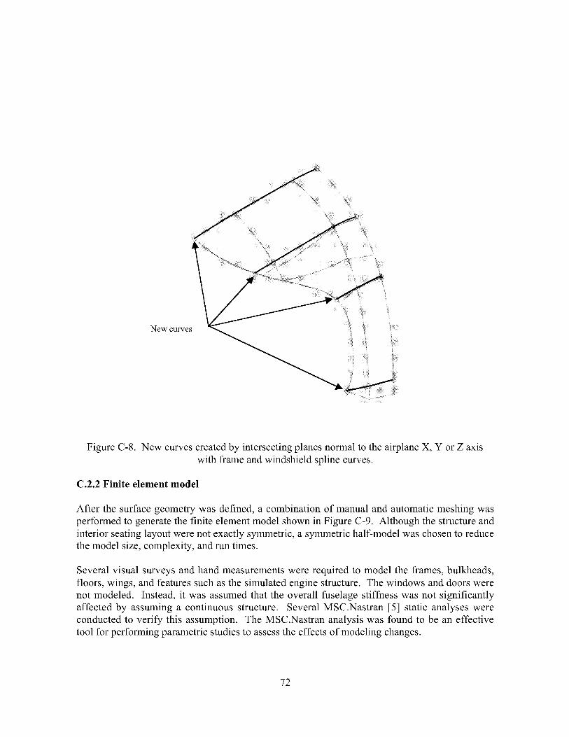
Newcurves _ _ :

FigureC-8. New curvescreatedby intersectingplanesnormalto theairplaneX, Y or Z axiswith frameandwindshieldsplinecurves.

C.2.2Finite elementmodel

After thesurfacegeometrywasdefined,a combinationof manualandautomaticmeshingwasperformedto generatethefinite elementmodelshownin FigureC-9. Althoughthestructureandinteriorseatinglayoutwerenotexactlysymmetric,a symmetrichalf-modelwaschosentoreducethemodelsize,complexity,andruntimes.

Severalvisual surveysandhandmeasurementswererequiredto modeltheframes,bulkheads,floors,wings,andfeaturessuchasthesimulatedenginestructure.Thewindowsanddoorswerenot modeled. Instead,it wasassumedthatthe overallfuselagestiffnesswasnot significantlyaffectedby assuminga continuousstructure. SeveralMSC.Nastran[5] static analyseswereconductedto verify this assumption.TheMSC.Nastrananalysiswasfoundto beaneffectivetool for performingparametricstudiesto assesstheeffectsof modelingchanges.

72

FigureC-9. Finiteelementmodelof theLearFanaircraft(symmetrichalf-model).

Limited dimensionalinformationwasobtainedfrom originalLear Fandesignlayoutdrawingsandtechnicalpapers.Consequently,anultrasonicthicknessgagewasusedto mapthefuselageskinthickness.Thisprocesswastime-consumingandtedious,andit provedto beimpracticaltoapply theresultsdirectlyto the finite elementmodeldueto ill-definedcontours.Instead,thethicknessmeasurementswereusedto verify informationobtainedfrom technicalpapersandpreviousanalyses,andto modify thebaselinethicknessin areaswherethedirectmeasurementsweretheonly sourceof information.

Finiteelementmesheswerecreatedto modelthefuselageandinterior framesasshellelements.Somestiffeners in areasoutsideof the passengercompartmentwere modeledwith beamelements.Lumpedmasseswereusedto representaddedmass,suchassimulatedenginemasses,instrumentationandequipment.

Since wing modeling was not a major concernin terms of structural damage(post-testinspectionsrevealedthat thewing wasnot severelydamaged),a simplifiedwing modelwasgeneratedto obtainthepropermassdistributionandto accountfor realisticdynamicstructuralinteractionwith thefuselage.Thewingmodelwasconvertedto MSC.Nastranformat,andbothstaticandnormal-modesanalyseswereperformedto verify the stiffnessandmassproperties.Theresultswerecheckedagainstanequivalentbeammodel(alsoconvertedto MSC.Nastran)ofthewingthathadbeendevelopedin apreviousLearFanstudy[6].

Theenergyabsorbingsubfloorbeamsweremodeledseparately(seeReferences7, 8, and9) andthenintegratedinto theMSC.Patranairplanemodel. Thesubfloormodelhadto bereadinitiallyinto a MSC.Patrandatabasewith the Nastran-preferenceactiveand then convertedinto a

73

MSC.Patrandatabasewith theDytran-preferenceactivein orderto properlyreadin the localcoordinatesystemfor thesubfloor.Unfortunately,dueto problemswith theprocessorthatreadsbulk datainto anMSC.Patrandatabase,thePCOMPmaterialpropertieshadto be inputinto theMSC.Dytranmodelvia an"include"file. Theintegrationprocessalsoprovedto becomplicateddue to the conflicting constraintson node spacingdictatedby the cellular designof thecompositebeamsand the fixed location of the aircraft frames. A view of a typicalsubfloor/framemodelingdetailis shownin FigureC-10. Thebeamwassubdividedinto fourelementsin theprimary load-carrying(vertical)directionin orderto adequatelysimulatetheexpectedcompressiveresponsewith aminimumnumberof elements.If thebeamshadexhibitedmorecrushingduringthetest,themeshwouldhaverequiredsignificantlymorerefinement.

The analysiswas focused on the structural responseof the aircraft. Therefore, theanthropomorphicdummieswere not explicitly modeledor analyzed. Initial versionsof theMSC.Dytranmodeldidnot includemodelsof theaircraftseats.Insteadthecombinedseatsanddummiesweremodeledaslumpedmassestied to thesubfloorbeamsby stiff beamelements.Seatmodelswereintroducedinto laterversionsof theaircraftmodel.

Rigidseatmodel

i!i

Energy absorbingseat model

Figure C-10. Passenger and subfloor beam modeling detail.

The MSC.Dytran model representing half the fuselage was comprised of about 25000 elements,

primarily CQUAD4 quadrilateral, single-integration-point, Key-Hoff shell elements. Beam

elements were used to simplify modeling in non-critical locations, and solid elements were usedto model the foam core of the subfloor beam cells. Element dimensions were limited to about 1

2 inches in the refined fuselage region. This size was chosen to provide sufficient

displacement and stress resolution while maintaining a time step of about one microsecond. For

74

the symmetrichalf-modelthis resultedin run times of about 12 15 hours to simulate 0.020

seconds on a Sun Ultra 450 Enterprise workstation computer.

Most of the aircraft fuselage shell structure was comprised of a graphite-epoxy composite

material. Flat bulkheads and floors were made of honeycomb sandwich material with composite

face sheets. Simplified material models were used wherever possible. The quasi-isotropic

layups of the fuselage skin and frames were modeled as isotropic elastic-plastic (DMATEP)

materials with no strain hardening. Material properties were derived from tensile tests of

coupons taken from the first and second Lear Fan fuselages. Kindervater performed a more

detailed analysis of the composite material behavior, including a progressive failure mechanism

and different moduli in tension and compression [10]. This approach was not used due to limited

resources for testing, and due to the lack of support in MSC.Dytran for bimodular materials that

have different moduli in tension and compression. A study was conducted to validate the

assumption that the graphite-epoxy material properties derived from the tension tests could be

used to predict bending failure. Mesh density issues were also investigated in the study, which is

presented in Reference 11.

The concrete impact surface was modeled as a single layer of solid elements 20 inches thick. A

contact surface was defined using the top surface of the concrete as the master surface and the

bottom fuselage grid points as slave nodes. Early simulations showed that the wing was

displacing through the keel beam, so a second contact surface was defined to allow the bottom of

the wing to contact (and crush) the composite keel beam. This modification reduced unrealistic

deformation in the rear fuselage.

MSC.Dytran does not compute the rigid-body mass properties of a flexible analysis model;

however, the code can be "tricked" into performing this calculation by converting all material

properties into "MATRIGs" and converting "PCOMPs" into "PSHELLs." This process

generates rigid bodies grouped by elements that have the same material property numbers. A

"PARAM,MATRMERG,AUTO" card is inserted into the bulk data deck to tell the code to

assemble all the rigid bodies into a single rigid body. A check run can then be executed to

compute the rigid body mass properties of the entire model.

An alternative to calculating the properties in MSC.Dytran is to use the "Mass Properties Tool"

in MSC.Patran. This method is much easier to use than the MSC.Dytran method because no

model modifications are required. In addition to the ease of use, MSC.Patran also offers the

convenience of output in a user-specified coordinate system as well as graphical output showing

the orientation and location of the principal mass axes. The results can be written to a text file.

Unfortunately, the "Mass Properties Tool" does not account for the mass of beams whose

properties are computed automatically by MSC.Patran, including the new beam sections that

have been added to the Dytran preference. Also, any elements or properties that are manually

edited into the MSC.Dytran analysis deck will not be included, because they are not present in

the MSC.Patran database. Both of these problems were encountered in the Lear Fan model.

Therefore, the MSC.Patran output was used as an estimate of the exact properties.

Impact velocities were determined by analyzing the high-speed video of the test. These initial

velocities were then input into the simulation. The initial translational velocities were 31 ft/sec

75

in the vertical directionand 82 ft/sec in the horizontaldirection. Thependulum-swingtesttechniqueusedatthe ImpactDynamicsResearchFacility for performingfull-scalecrashtestsintroducesarigid bodyrotationalvelocity, estimatedto be 0.494radians/secondfor theLearFan test (pitch angularvelocity, nose-up). This rotational velocity was accountedfor bycomputingthetranslationalcomponentsateachgrid pointin themodelandthenaddingthemtothetranslationalvelocitycomponentsof thecenter-of-gravity.SinceMSC.Dytrandid nothaveaconvenientmethodof performingthis initialization,ausersubroutinewasdevelopedto performthesecomputations.

C.2.3 Simulation results

The Lear Fan aircraft, seats, and test dummies were instrumented to measure occupant responses

and to evaluate new structural concepts, e.g. the composite energy-absorbing subfloor.

Correlation with analytical models was a secondary goal, so structural response measurements

were limited. Therefore, the emphasis of the analytical effort was focused on simulating the

structural damage that could be verified by recorded images, including the primary damage to

the fuselage that was observed at the wing attachment locations, where cracks initiated in the

skin and rapidly progressed to the crown, essentially breaking the fuselage into two pieces.

Attempts were also made to correlate some of the vertical accelerations near the seat attachment

points, since these accelerations are typically measured to estimate the dynamic inputs to theseats.

Plots of the deformed model are shown in Figure C-11 for simulation times at 0.005-second

intervals. The frame damage observed in the post-test inspections is evident as early as 0.005

seconds, and by the time the simulation has ended (at t=0.020 seconds), several frames have

failed at or near the longitudinal centerline. The fuselage damage in the highly loaded region

near the baggage compartment and the wing box is also evident as early as 0.010 seconds. In

Figure C-12 the circumferential fuselage damage that initiated at the forward wing attachment

location can be seen in the deformation plot. This damage matches closely the circumferential

fuselage "unzipping" seen in the high-speed video.

Early versions of the simulation model did not account for the crushing of the keel beam. The

deformed structure, shown in Figure C-13, showed interference between the wing and the keel

beam, indicating that there should be contact between these two components to properly transmit

the forces from the wing into the keel beam. The large deformation at the fuselage crown is

caused by the downward wing forces that are not dissipated by contact with the keel beam. After

the wing-keel beam contact was included in the model, the crack at the aft wing attachment

location does not appear in the simulation, possibly because the wing has not yet hit the concrete

impact surface. It is possible that the fuselage model is too stiff or too damage-resistant;

however, it is difficult to validate these hypotheses with the limited experimental data available.

76

iilli_iiiii_ii_i!ii!_i!iiii!!iiiiiiii!iiiiiiiiii!iiiii_i_!iii!i!iiii%i¸¸_¸¸_¸¸

typical frame damage

(note: missing

have failed)

T = 0.005 sec T = 0.010 sec

Figure C-11. Deformed structure plots (true scale) at 5, 10, 15 and 20 milliseconds.

Early simulations generated excessive crushing of the composite subfloor beams. This behavior

did not match the test results. A closer examination of the video footage from the interior

cameras revealed that the seats, especially the energy-absorbing seats, deformed significantly on

initial impact. This feature was not accounted for in the simulation, because the seats had been

modeled only as very stiff beams, with a lumped mass to represent the combined seat and

passenger mass. In order to assess the effects of seat deformation, a finite element model was

created of an energy-absorbing seat. This approximate seat model was integrated into the Lear

Fan model, and a new simulation was performed. The difference in the amount of subfloor beam

crushing indicates clearly that the seat flexibility has a significant effect on the response of the

subfloor. The primary locations of interest in the simulation were the pilot and copilot seats.

For these locations, the simulation predicted an initial peak filtered acceleration of about 190 g's,

compared with the experimental value of 200 g's. As mentioned previously, the acceleration

data were filtered using a 200-Hz low-pass digital filter. Inspection of deformed structure plots

suggests that the second large pulse in the analysis plot was probably caused by the approximate

seat modeling [10, 11 ].

77

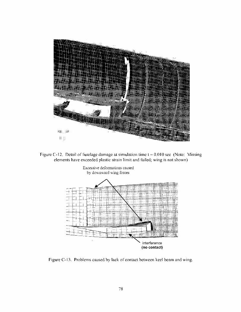
FigureC-12.Detailof fuselagedamageatsimulationtimet = 0.010sec(Note: Missingelementshaveexceededplasticstrainlimit andfailed;wing isnotshown)

Excessivedeformationscausedbydownwardwingforces

interference(no contact)

Figure C- 13. Problems caused by lack of contact between keel beam and wing.

78

C.3 Lessons Learned

Please note that the comments in this section on modeling and analysis code capabilities refer to

the software versions used in the Lear Fan modeling and analysis (MSC.Patran Version 9.0 and

MSC.Dytran 2000). Some of the problems discussed have been eliminated in later versions ofthe software.

C.3.1 Geometry model development

The following is a list of recommended practices that are based on the development of the

geometry model of the Lear Fan crash simulation.

(1) Confirm/correct the orientation (and location) of the airplane geometry, as defined by the

photogrammetric survey data, before generating higher level geometry and finite elementmeshes.

(2) Use photogrammetric points to create frame curves; then use user-defined cutting planes to

create longitudinal curves for generation of smooth, compatible surfaces.

(3) Ignore initial frame geometry, and instead use known frame locations to create correctly-located frame curves.

(4) MSC.Patran may not be the best or easiest tool to use to create surface geometry based on the

photogrammetric survey data. Other tools to consider are the NASA LaRC GEOLAB services

or CAD software such as Pro/Engineer.

(5) MSC.Dytran does not allow output in coordinate systems other than the global XYZ system.

Since accelerometer data is referenced to a moving coordinate system, the assumption is

frequently made that the orientation of the accelerometer does not change during the short-

duration impact. This assumption may not always be valid.

C.3.2 Finite element model development

The following is a list of recommended practices that are based on the development of the finiteelement model of the Lear Fan crash simulation.

(1) Careful consideration should be given to devising efficient methods of connecting meshes

developed independently for various model components. In some cases, it may be advantageous

to use connection elements such as RCONNs to tie the two meshes together. This method would

have simplified the connection of the subfloor model to the fuselage model, because it would

have eliminated the need to have the fuselage mesh be compatible with the subfloor mesh.

(2) MSC.Nastran static analysis was useful in assessing the effectiveness of various structural

modeling techniques. Static analyses can be executed and post-processed much more rapidly

than transient dynamic analyses, enabling an analyst to investigate several modeling alternatives

in the same amount of time that it would take to perform a single MSC.Dytran transient analysis.

(3) The MSC.Patran bulk data reader did not input correctly all of the material and property datawritten for the subfloor beam.

(4) The MSC.Patran bulk data reader was not able to process a local coordinate system, when a

bulk data file was read into a new Dytran-preference database.

(5) MSC.Patran does not account for the mass of beams that do not have explicitly-defined

section properties, when it calculates rigid body mass properties.

79

(6) MSC.Dytrandoesnot computethe masspropertiesof analysismodelsunlesstheyconsistonly of a singlerigid-bodyelement.Temporarymodificationof themodelis aworkaroundforthisproblem,but it requiresconsiderablecareandeffort.(7)MSC.Dytrandoesnot featureaneasymethodof applyingrigid-bodyinitial angularvelocitiesto aflexible simulationmodel. An externalsubroutinehadto bedevelopedto accomplishthistask.Themethodrequiresknowledgeof thecenter-of-gravitylocation.An alternativewouldbeto useMATRIGsto convertthemodelto arigid bodyandapplythe initial conditions.After thesimulationhasrun for afew timesteps,but beforethemodelhascontactedtheimpactsurface,theMATRIGscanbe removed,andarestartcanbeperformedusingtheflexiblemodel. Thismethodis rathercumbersometo use,sinceit requiresmodelmodificationsandrestarts.(8)MSC.Dytrandoesnothavematerialmodelssuitablefor asimplebimodularmaterial,i.e.onethathasadifferentmodulusin tensionandcompression.(9) Finiteelementmeshrefinementsmaybe limitedby theneedto maintainareasonablylargetime step. Experiencehasshownthat limiting theminimumtime stepto approximatelyonemicrosecond(le-6 seconds)is agoodrule of thumb. For stiff, lightweightmaterialssuchascomposites,theresultingelementsmaybetoolargeto accuratelypredictstresses.(10) Caremustbe takenin selectinganappropriateoutputtime stepfor accelerations.Therelativelyhigh-stiffness,low masselementsthat areusedtypically in a compositestructuralmodelmayhaveveryhighnaturalfrequencies.For example,a 1-inchsquareflat platemadeofLearFanfuselagematerialwouldhavenaturalfrequenciesontheorderof 10-20Khz. In orderto preventaliasingof the data,theaccelerationswouldhaveto besampledat greaterthan40Khz, accordingto thecommonlyusedNyquistcriteria. Samplingat thesamefrequencyastheexperimentaldata(e.g.,10Khz for theLearFantest)mayproduceincorrectresults.A work-aroundfor thisproblemis to selectoutputlocationsthathavealumpedmassassociatedwiththemor to addsmallmassesto structuralnodes.Themasslowersthenaturalfrequenciesatthesamplinglocation,enablingalargersamplingperiod,with associatedsavingsin file size

C.4 References

1. Hart-Smith, L.J., "Design and Development of the First Lear Fan All-Composite Aircraft,"

McDonnell Douglas, Douglas Paper 8184, presented to Institution of Mechanical Engineers

Conference on Design in Composite Materials, London, England, March 7-8, 1989

2. Carden, Huey D. and Kellas, Sotiris, "Composite Energy-Absorbing Structure for Aircraft

Subfloors," Tenth DoD/NASA/FAA Conference on Fibrous Composites in Structural Design,Hilton Head, SC, November 1993.

3. Jones, L. E., and Craden, H. D., "Overview of Structural Behavior and Occupnat Responses

from a Crash Test of a Composite Airplane," SAE Paper 951168, presented at the SAE General,

Corporate and Regional Aviation Meeting and Exposition, Wichita, KS, May 3-5, 1995.

4. MSC.Patran Users Manual, Version 2000, MSC.Software Corporation, Los Angeles, CA,1999.

5. MSC.Nastran Quick Reference Guide, Version 70.7, MSC.Software Corporation, Los

Angeles, CA, 1999.

80

6. Dykman,J.R., "Lear Fan 2100Impact DynamicsAnalysis EngineeringReport,"ReportNumberR45108,LearFan,Reno,N.V., April 22,1985.

7. Knight,NormanF.,Jr.,Kellas,Sotiris,andPinson,LarryD., "PredictingtheImpactResponseof anEnergy-AbsorbingCompositeSubfloorBeam,"AIAA PaperNo. 2000-1472,presentedatthe 41st AIAA/ASME/ASCE/AHS/ASC Structures,Structural Dynamics, and MaterialsConference,Atlanta,GA,April 3-6,2000.

8. Knight, NormanF., Jr.,Kellas, Sotiris,andPinson,Larry D., "CompositeSubfloorBeamSimulationsUsingMSC/Dytran,"VeridianMRJTechnologySolutions,September1999.

9. Knight,NormanF., Jr., "CrashSimulationSupport,"VeridianMRJ TechnologySolutions,August2000.

10. Kindervater,C.M., "Aircraft and HelicopterCrashworthiness:Designand Simulation,"Crashworthiness of Transportation Systems: Structural Impact and Occupant Protection,Kluwer Academic Publishers, Netherlands, 1997.

11. Stockwell, A., "Evaluation of Modeling and Simulation Tools and Techniques for an

Analytical Study of the Lear Fan Impact Test," NASA CR-2002-211457, March 2002.

81

APPENDIX D. SIMULATION OF A COMPOSITE FUSELAGE SECTION WITH

ANTHRPOMORPHIC DUMMIES AND ENERGY-ABSORBING SEATS

D.1 Experimental Program

D.I.1 Test set-up

An innovative and cost-effective composite fuselage concept was developed at NASA Langley

Research Center to meet structural and flight loads requirements and to provide improved crash

protection. The composite fuselage concept consists of a stiff upper fuselage, a structural floor,

and an energy-absorbing subfloor. The upper section of the fuselage cabin is fabricated using a

composite sandwich construction and is designed to provide a protective shell that encloses the

occupants in the event of a crash. The energy-absorbing subfloor is designed to dissipate kinetic

energy through stable crushing. Finally, a key feature of the fuselage concept is the stiff

structural floor. The structural floor is designed to react the loads generated by crushing of the

subfloor, and to provide a stable platform for seat and restraint attachment.

A 5-ft diameter fuselage section was fabricated, as shown in Fig. 1, and impact tests were

performed at 25 ft/s vertical velocity. The upper section of the fuselage is fabricated using acomposite sandwich construction with a 3-1b/ft 3 closed cell polyurethane foam core and E-

glass/epoxy fabric face sheets. The composite sandwich construction in the floor of the fuselage

consists of an 8-1b/ft 3 closed-cell polyurethane foam core with hybrid face sheets consisting of E-

glass/epoxy and graphite/epoxy composite fabric. The layers of graphite/epoxy fabric were

added for increased stiffness and improved structural rigidity. The energy-absorbing subfloor

configuration is a geometric foam-block design, consisting of five, 6.5-inch deep uniformly

spaced, individual blocks of a crushable Rohacell 31-IG (Industrial Grade) 2.8-1b/ft 3 closed-cell

foam overlaid with E-glass/epoxy face sheets. The geometry of the foam blocks, shown in

Figure 1, was chosen to maintain a fairly uniform cross-sectional area as the crush zone develops

and progresses vertically, resulting in a fairly constant crushing force. Details of the composite

fuselage section design and fabrication can be found in reference [1].

Fig. 1. Composite fuselage section pre-test.

82

A plan-viewof thefloor is showninFigure2thatindicatesthelocationof theseats,leadmasses,dummyfeet,andaccelerometersusedfor test/analysiscorrelation.Pre-testphotographsof thefuselagesectionwith dummyoccupantsareshownin Figure1. Theemptysectionweighed200lbs. Leadblockswereplacedonthefloor to bringthetotal sectionweight,includingtheseatsanddummies,to 1,243pounds.The fuselagesection,seats,anddummieswereinstrumentedwith 80 transducersto recordthe dynamicresponseof the impact. Thefuselagesectionwasraisedto aheightof 10feetanddroppedontoa rigid surfaceto achieveanimpactvelocity ofapproximately25 ft/s. Thedatawererecordedat 10,000samples/secondusinganon-boarddigital dataacquisitionsystem.The 50 th percentile male Hybrid II dummies had lumbar load

cells installed to measure the spinal force response. In addition, load cells were placed under

each seat leg, and accelerometers were placed on the floor and circumferentially around the

fuselage. Each test dummy was secured in his seat with a conventional lap belt and shoulder

harness. Each dummy was instrumented with 9 accelerometers, three in the head, chest, and

pelvis to record accelerations in the forward, side, and vertical directions.

• - Accelerometers(used for correlation)

• - Seat leg attachment

- lO0-1b, lead mass

O - Dummyfeet hell

Front

cLAL _

x )<Rear

Fig. 2. Floor layout of the seats, dummies, instrumentation and ballast weight.

The energy-absorbing seats used in the test were Jungle Aviation And Radio Service (JAARS)

seats, which consist of a steel tubular frame with an S-shaped front leg. The development of the

JAARS seat concept began in the 1980's. Prior to in-service use, prototype JAARS seats were

tested in dynamic sled tests and in full-scale crash tests of general aviation aircraft at the Impact

Dynamics Research Facility located at NASA Langley Research Center [2].

D.1.2 Summary of test results

The vertical acceleration time-histories from the left dummy pelvis and the inboard and outboard

seat track accelerometers on the rear lead mass just behind the left seat are plotted in Figure 3.

Note that the floor acceleration pulse duration is approximately 0.035 - 0.04 seconds. The onset

of the dummy pelvis acceleration lagged the onset of floor acceleration by approximately 0.005

83

seconds,and the durationof the pelvis accelerationis about 50 % longer than the flooracceleration.Thefloor accelerationinitially peaksaround40to 50-gandthenlevelsoff between30 and 35-g. The stroking of the energy-absorbingseatlengthensthe width of the pelvisaccelerationpulseandlowersthe effectiveaccelerationof the dummypelvis to below 20-gexceptfor thelocalizedpeakof 30-gthatoccursnear0.047seconds.

Acceleration, glOO .........

ii ill iI- i i ..... Outboard track

60 [ ..... Inboard track

i '_ i i

40 --#--_,-i..........i....................................................................

]- i i -i i :

0 r. i

i ".."i

-20 0 ....... 0'.{)'2..... 0'.0'4 ' 0'.b'6..... 0'.08

Time, s

Fig. 3. Comparison of floor-level and left dummy pelvis acceleration.

The lumbar load measured at the base of the spinal column can be used to predict spinal injury.

To prevent or limit injury to the spine, FAR Part 27.562c [3] stipulates that the lumbar load

should not exceed 1,500 pounds. The lumbar loads for each dummy are plotted in Figure 4. The

peak lumbar load measured in the pelvis of the right dummy is slightly less than 1,500 pounds,

while the peak load measured in the right dummy pelvis was slightly over 1,500 pounds.

Consequently, the objectives of FAR Part 27.562c were met for the right dummy and were

almost met for the left dummy.

D.2 Description of Modeling Approach

MSC.Dytran [4], a general-purpose explicit nonlinear transient dynamic finite element code, wasused to model the composite fuselage section and the JAARS seats. The 50 th percentile male

Hybrid II anthropomorphic dummies were modeled using the Articulated Total Body (ATB)

code [5]. ATB is an independent computer code developed by the Air Force Wright Laboratory

as a numerical dummy model, and it is integrated within the MSC.Dytran program. The ATB

dummy model consists of hinged segments with inertias, joint properties, and contact surfaces

defined to represent a Hybrid II dummy. A picture of the integrated MSC.Dytran model of the

fuselage section with two JAARS seats and two seated ATB dummies is shown in Figure 5a, and

a cut-away view of the right half of the model is shown in Figure 5b. The MSC.Dytran model of

the 4130 annealed steel seat frames, shown in Figure 5c using MSC.Patran's 3-D visualization,

were modeled with beam elements, which were defined with elastic-plastic material properties.

84

Load, Ibs x 1000

0.5

0

-0.5

-1

-1.5

Left dummy I ,,i

--_--Right dumrny li ......

-20 0.02 0.04 0.06 0.08 0.1

Time, sec

Fig. 4. Left and right dummy lumbar loads, unfiltered.

The modulus of the steel was 2.97e07 psi, the yield stress was estimated to be 5.2e04 psi, and a

strain hardening modulus of 1.0e06 psi was assumed. The ATB dummy segments are covered

with rigid shell elements in MSC.Dytran to provide the correct body contour needed for contact

calculations. The seat cushion forces were modeled in ATB using linear force-deflection

segments. Each dummy model consisted of 3,069 nodes and 3,207 elements.

A three-dimensional finite element model of the full-scale fuselage was developed using the pre-

processing software, MSC.Patran. The model was executed in MSC.Dytran Intel Linux Version

2001. Excluding the dummies, the complete section model consists of 27,408 nodes and 32,811

elements. The elements in the fuselage section structure included 13,317 shell elements, 18,796

solid elements; 698 beam elements representing the seats and seat rails, and 48 concentrated

masses representing the lead floor masses and ballast weights. The inner and outer face sheets of

the upper section and floor were modeled using 4-noded Belytschko-Lin-Tsay shell elements,

and the foam core in the upper section, floor, and subfloor was represented by 8-noded

hexagonal solid elements. Contact regions were defined between the section and the impact

surface, between the seat and the floor, between the dummy and the seat cushions, and between

the dummy's feet and the floor.

85

;<<<<<<<<<<<<<<<<<<<<<<<<<<<<<<<<<<<<<<<<<<<<t ¸¸ ;

(a) Front view full model (b) One-half cut of the model

(c) Seat frame model, 3-D beam visualization

Fig. 5. Finite element model.

The material properties of the E-glass/epoxy fabric material were determined from coupon tests

and are modeled using a bilinear elastic-plastic material model with strain hardening. The 3- and8-1b/ft 3 polyurethane foam cores in the upper section and floor were modeled as linear elastic

solid materials. The more complicated multi-layered face sheets in the floor were modeled as

laminated composite shell elements (PCOMP) in MSC.Dytran. The material model for the five

6.5-in.-deep Rohacell foam blocks, which are located in the subfloor region of the finite element

model, were obtained from crushing tests of individual cubic blocks of foam. The Rohacell was

represented as crushable foam (FOAM2) with the stress-strain response provided in a "look-up"

table. The table was determined directly from the experimental data, and stress values were

provided versus volumetric crush. The bulk modulus of the Rohacell foam is based on the

maximum slope of the stress-strain response to provide for numerical stability. The FOAM2

material model is used in MSC.Dytran for a crushable, isotropic foam material with a user-

specified hysteresis response for unloading and a Poisson's ratio that is effectively zero. An

exponential unloading curve and a 74.2-psi tensile cutoff stress were specified in the current

model, as shown in Figure 6. The energy dissipation factor in FOAM2 was set to 0.99.

86

Stress, psi

...... i i ' '

200 ' ' ' Exponential i '/

150 , unloading i

loo

500 I_I.............Compressiveii...............ii................responseii............

Tensile

-50 i / cut-off _stressi i i i

-100,,, i,,, i,,, i,,, i , , ,-0.2 0 0.2 0.4 0.6 0.8

Crush

Fig. 6. Quasi-static crushing response of Rohacell foam.

A master-surface to slave-node contact is defined between the subfloor and the impact surface,

which is modeled as a thick plate with all of the edge nodes fixed.

The ATB model included the seat reference system, the cushioning material of the seats, plus the

two 50-percentile Hybrid II dummies. The dummies were positioned in the seats using

MSC.Patran. The input to the ATB code was in a separate file with fixed formatting. The seat

cushioning material was given a bi-linear curve to represent the seat cushions, plus a bottoming-

out curve that would cause the seat structure to deform as designed. The initial slope for the seat

bottom cushion was set to 500 pounds per inch. After three inches deflection, the bottoming-out

slope of the cushion was set to 1500 pounds per inch. The seat back cushion was modeled as

much stiffer than the bottom cushion with an initial slope of 1000 pounds per inch. Since the

impact is vertical, no restraints were modeled since the restraints see very little load in the test.

The unloading curves for the seat cushions are also very important and must be modeled to

capture the energy dissipated and to prevent elastic rebound. The ATB code also allows friction

between the dummy and the seat cushion to be modeled. A friction coefficient of 0.62 was

assumed. Also, in ATB, the cushion was assumed to absorb all of the energy (vertical unloading

path). The permanent set of the cushion was input as 0.80 of the original cushion depth.

An initial vertical velocity of 300 in/s (25 ft/s) is assigned to all nodes in the model except for

those nodes forming the impact surface. More details on the structural model of the fuselage can

be found in references [6,7,8]. The model was run on one processor of an Intel Linux two-

processor, 1.7 GHz workstation. To simulate 0.07 seconds required about 5.5 CPU hours.

D.3 Lessons Learned

This model, which includes the fuselage, seats, and dummies, is complicated due to the complex

motion and interactions of the different objects that compose the test article. The fuselage

weighs approximately 200 pounds. The ten lead masses weigh 1000 pounds. Each seat and

dummy combination weighs almost 200 pounds. The seat provides the coupling between the

87

fuselageanddummy. Theseatcushionprovidesthe initial couplingbetweenthedummyandseat. Consequently,the seatmustbeaccuratelymodeledto obtaingoodresults.Althoughthetestarticleis staticallybalanced,it is notdynamicallybalanced.Onimpact,thedummymassiscoupledto thefloor throughthestrokingseat.In effect,theforceappliedto thefloor throughtheseatis lessthanif thedummymasswereattachedto thefloor. Consequently,thesectionpitchesforwardduringtheimpactasthedummymassis behindthestaticcenterof gravity. In addition,theseatcushioningmaterialishighlynonlinearandmustbecompressedbeforethedummywillloadtheseat.

Thematerialpropertiesof the4130-alloysteeltubingfor theseatsarecriticalin obtaininggoodresults. The MSC.DytranmaterialmodelselectedwasDMATEP. Thevaluesusedfor thispartiallyannealedalloy was52,000psi yield, anda strainhardeningvalueof 1.0e6psi. Steeloftenhasa complexstress-strainbehaviorwhenit exceedstheelasticlimit oryield. If practical,coupontestingwouldhavebeenperformed;however,nomaterialwasavailablefor testing. ThesubfloorRohacelfoamwasmodeledin MSC.Dytranasa FOAM2material. Thefoamloadingwasinput asatableof engineeringstressversuscrush.Thecrushis thechangein volumeovertheoriginalvolume. Theunloadingcurveof a foammaterial,or for anynonlinearmaterial,isextremelyimportantto capture.Theunloadingcurveshapeandtheenergydissipatedwerebothspecifiedfor theRohacelfoam. Theunloadingcurveshapewasdefinedto beexponentialandthe energydissipatedwas assumedto be 0.99. Thus, there is very little hysteresisin theunloadingcurve.Althoughthevalueof 0.99is likely greaterthantheactualenergydissipated,itis practicalto startthemodelwith a largevaluefor the energydissipationfactor. Whenthemodelwas first run, a smallervalueof 0.8wasusedfor the energydissipationfactor for theRohacelfoam.However,this valueallowedelasticenergyto be returnedto the sectionandresultedin excessiverebound.

Comparisonsbetweentestandanalysisweremadewith accelerationresponsesmeasuredonthelargeleadmasses.In Figure7, thetwo symmetricrearinboardaccelerometerson the 100-lb.leadmassesarecomparedwith themodelpredictions.Theleft inboardaccelerometerexhibitsapeakof 50-gwhile theright inboardaccelerationis lowerat 43-g. In addition,althoughthemodelwassymmetric,the left andright rearinboardaccelerationsarenot identical. Thepeaksof theanalyticaldatarangefrom 49-gto 53-g. However,both analyticalaccelerationpulsesexhibit a secondpeakafter0.02secondsthat is considerablyhigher thanin the experimentaldata.

88

Acceleration, g

60 ! r --_-- Exp., left•-_ -Exp., right

[ -_; • --*--Analysis, left50 /y,._; ..... Analysis, right

40 - "........

30 i i 'i ......._........i .................{.................

2010

[ I °'_ . i

i o%'oi

0 _ _-

-10 _ L J L i '_ ,0 0.01 0.02 0.03 0.04 0.05

Time, s

Fig. 7. Comparison of experimental rear inboard accelerations with model results.

In Figure 8, the pelvis acceleration of the ATB model is compared with the left dummy pelvis

vertical acceleration response. As shown in the figure, the ATB model predicted the overall

shape, pulse duration, and maximum acceleration quite well. The predicted peak pelvis

acceleration was 24-g, as compared with an experimental acceleration that oscillated about 20-g

for 0.02 seconds before peaking locally at 30-g. The final peak in the dummy acceleration may

have been due to the seat "bottoming-out."

Acceleration, g40

30

20

10

-10

Experimen{ l--*--ATB model

.01 .02 .03 .04 .05

Time,s

--_ ............. i

:¢

i.06 .07

Fig. 8. Measured left dummy pelvis vertical acceleration compared with the Dytran/ATB

predicted pelvis acceleration.

89

Motion picturedataselectedfrom framestakenat approximately0.0025-secondintervals(400frames/second)arecomparedqualitativelywith themodelbehaviorin Figures9. Themotionpicturedatashowthatthefront endof thesectionimpactedwith lessthanone-degreedownwardpitch. This initial pitch anglewasnot includedin themodel.Thefront view showsthat thedummyandseatmodelsfollowtheactualmotionquitewell.

Thecomparisonof theside-viewcameraframeswith thepredictedmotionshowthefront of thesectionpitcheddown by 4 degreesat 0.05 seconds. Also, by 0.07seconds,the sectionisapproximatelylevelagain. The centerof gravityof thesectionandmodelwereboth locatedlongitudinallyin thecenter.Asmentionedbefore,thefront-enddownwardpitchis causedbytheactionof theseatsanddummies.Sincetheloadpathof thedummiesis throughthecrushableenergy-absorbingseats,which areactuallyload-limitingdevices,thedownwardforceappliedtothefloor by the seatlegsis lower thanif a rigid seathadbeenused. Consequently,sincetheseatsand dummiesarebehindthe center-of-gravity,a counter-clockwisepitching momentresults.

Themotionof theseatcanbeseenin thefront view in Figure9. Onecanobservethetworearside bracesof the seatbendingoutward. At time t=0.07 secondsthe seathasessentiallybottomedoutandthedummiesareverycloseto thefloor. Close-uppicturesof theright JAARSseattakenpost-testareshownin Figure10. Thedeformationof theS-shapedfrontseatlegsandthesupportstrapcanbeclearlyseenin thepictures.Thefront framesof theJAARSseatswereoriginally10inchesabovethefloor,while therearhorizontalseatframeswere9.5inchesabovethefloor. After thetest,thepermanently-deformedcomersof thefront seatmeasuredfrom 5.15-to 5.6-inchesabovethefloor,while therearflamecomersmeasuredfrom 6.875-to 7.65-inchesabovethefloor. Thusthefront of theflamestrokedabout5 inchesfor theright seatandabout4.5 inchesfor theleft seat,while thebackof theright seatstrokedabout2.5 inchesandthebackof the left seatstrokedabout2.0 inches.Recallfrom anexaminationof the lumbarloadcurvesin Figure4,thatthedummyin theright seatdidexperiencea smallerpeaklumbarload,whichisconsistentwith theseatstrokingdata.

90

t=.03

t=.05

iiiiii

t=0.07

Fig. 9. Front view comparison of high-speed film data with model.

Fig. 10. Deformed JAARS seats, post-test.

D.4 References

1. Jackson, Karen E., Fasanella, Edwin L, and Knight, Jr., Norman F., "Demonstration of a

Crashworthy Composite Fuselage Concept." Proceedings of the 22 ndArmy Science Conference,

Baltimore, MD, December 11-13, 2000.

91

2. Williams, M. Susanand Fasanella,E. L., "CrashTestsof Four Low-Wing Twin-EngineAirplaneswith Truss-ReinforcedFuselageStructure."NASA TP2070,1982.

3. Codeof FederalRegulations,FederalAviation Regulationsfor Aviation MaintenanceTechniciansFAR AMT, Part27AirworthinessStandard:NormalCategoryRotorcraft,27.562EmergencyLandingDynamics4. MSC.Dytran User's Manual Version 4. 7, Volumes 1 and 2.

MSC Software Corporation, Los Angeles, CA, 1999.

4. MSC.Dytran User's Manual Version 4.7, Volumes 1 and 2. MSC Software Corporation, Los

Angeles, CA, 1999.

5. Obergefell, L. A., Gardner, T. R., Kaleps, I., and Fleck, J. T., Articulated Total Body Model

Enhancements, Volume 2: User's Guide. AAMRL-TR-88-043, January 1988.

6. Fasanella, E. L., and Jackson, K. E., "Analytical and Experimental Evaluation of Composite

Energy-Absorbing Subfloor Concepts," American Helicopter Society National Technical

Specialists' Meeting on Rotorcraft Crashworthiness, Phoenix, AZ, September 14-17, 1998.

7. Jackson, K. E., and Fasanella, E. L. "Crashworthy Evaluation of a 1/5-Scale Model CompositeFuselage Concept," 55 th American Helicopter Society Annual Forum and Technology Display,

Montreal, Canada, May 25-27, 1999.

8. Jackson, Karen E., Fasanella, Edwin L, and Knight, Jr., Norman F., "Demonstration of aCrashworthy Composite Fuselage Concept." Proceedings of the 22 ndArmy Science Conference,

Baltimore, MD, December 11-13, 2000.

92

REPORT DOCUMENTATION PAGE Form ApprovedOAdBNo. 0704-0188

Public reporting burden for this collection of information is estimated to average 1 hour per response, including the time for reviewing instructions, searching existing datasources, gathering end maintaining the data needed, end completing end reviewing the collection of information. Send comments regarding this burden estimate or eny otheraspect of this collection of information, including suggestions for reducing this burden, to Washington Headquarters Services, Directorate for Information Operations endReports, 1215Jefferson Devis Highwey, Suite 1204, A#ington, VA 22202-4302, end to the Office of Menegement end Budget, Peperwork Reduction Project (0704-O188),Weshin_Iton, DC 20503.1. AGENCY USE ONLY (Leave b/an/0 2. REPORT DATE 3. REPORT TYPE AND DATES COVERED

October 2002 Technical Memorandum

4. TITLE AND SUBTITLE

Best Practices for Crash Modeling and Simulation

6. AUTHOR(S)Edwin L. Fasanella

Karen E. Jackson

7. PERFORMING ORGANIZATION NAME(S) AND ADDRESS(ES)

NASA Langley Research Center

Hampton, VA 23681-2199

9. SPONSORING/MONITORING AGENCY NAME(S) AND ADDRESS(ES)

National Aeronautics and Space Administration

Washington, DC 20546-0001

5. FUNDING NUMBERS

WU 728-50-10-01

8. PERFORMING ORGANIZATIONREPORT NUMBER

L 18223

10. SPONSORING/MONITORINGAGENCY REPORT NUMBER

NASA/TM-2002-211944

ARL-TR-2849

11. SUPPLEMENTARY NOTES

12a. DISTRIBUTION/AVAILABILITY STATEMENT

Unclassified-Unlimited

Subject Category 05 Distribution: Standard

Availability: NASA CASI (301) 621-0390

12b. DISTRIBUTION CODE

13. ABSTRACT (Max/mum 200 words)

Aviation safety can be greatly enhanced by the expeditious use of computer simulations of crash impact. Unlike

automotive impact testing, which is now routine, experimental crash tests of even small aircraft are expensive

and complex due to the high cost of the aircraft and the myriad of crash impact conditions that must be

considered. Ultimately, the goal is to utilize full-scale crash simulations of aircraft for design evaluation and

certification. The objective of this publication is to describe "best practices" for modeling aircraft impact using

explicit nonlinear dynamic finite element codes such as LS-DYNA, DYNA3D, and MSC.Dytran. Although

"best practices" is somewhat relative, it is hoped that the authors' experience will help others to avoid some of

the common pitfalls in modeling that are not documented in one single publication. In addition, a discussion of

experimental data analysis, digital filtering, and test-analysis correlation is provided. Finally, some examples of

aircraft crash simulations are described in several appendices following the main report.

14. SUBJECT TERMS

crashworthiness, aviation safety, nonlinear finite element modeling

17. SECURITY CLASSIFICATIONOF REPORT

Unclassified

18. SECURITY CLASSIFICATIONOF THIS PAGE

Unclassified

19. SECURITY CLASSIFICATIONOF ABSTRACT

Unclassified

NSN 7540-01-280-5500

15. NUMBER OF PAGES

9916. PRICE CODE

20. LIMITATIONOF ABSTRACT

UL

Standard Form 298 (Rev. 2-89)Prescribed by ANSI Std. Z-39-18298-102