best practices for automation and control of mine dewatering … · 2018-12-11 · cavitation....
TRANSCRIPT

Best practices for automation and control of mine dewatering systems
PJ Oberholzer
21696683
Dissertation submitted in fulfilment of the requirements for the degree Magister in Mechanical Engineering at the
Potchefstroom Campus of the North-West University
Supervisor: Dr JF van Rensburg
May 2015

Preface
i
Abstract
Title: Best practices for automation and control of mine dewatering systems
Author: Mr PJ Oberholzer
Supervisor: Dr J van Rensburg
Keywords: Best practice, automation, cavitation, overheating, efficiency, failure,
multistage centrifugal pump, control, schedule
Typical deep level mines use up to 27 ML water per day for mining operations. Multistage
centrifugal pumps up to 2500 MW are used in an upward cascading manor to dewater the
shaft. The dewatering systems at some mines are automated to enable surface control.
Automation of the pumps is typically based on the best practice procedure known when
implemented. Best practice procedures are used to ensure safe pumping operations. It was
found that pump failures could still occur even with the best practice implemented.
Unexpected failures of pumps are of major concern because they can result in the flooding
of a mine. Flooding increases the risk of environmental damage and injury to the mining
personnel. An additional concern is the maintenance cost of multistage centrifugal pumps.
Overhaul cost of a seized multistage centrifugal pump is almost R1-million.
The aim of this study was to improve established best practice procedures for pump
automation. This could be achieved by investigating the general root cause of failures of
automated pumps. Additional instrumentation and protection devices to prevent similar
incidents were examined. Revised system control parameters were developed to ensure that
the pumps operated within the design specifications.
The improved best practices proved to prevent failures as a result of overheating and
cavitation. Increasing the pump reliability and availability enabled surface control. The
control of the automated dewatering system realised an electricity cost saving of R6-million.
The automated system also made it possible to calculate the real-time pump efficiency within
5%.
Previous best practice procedure was found to be inadequate to prevent all possibilities of
failure. Additional precaution measurements were added to prevent pump failure.

Preface
ii
Acknowledgements
The research reported in this dissertation is my own work. Recognition was given to the
external sources used in the document. Any errors or omissions brought to the attention of
the author will be corrected.
I would like to thank our Lord, our Saviour for creating the earth and giving mankind the
responsibility to care for it.
Thank you to TEMM International (Pty) Ltd and HVAC International (Pty) Ltd for the
opportunity, financial assistance and support to complete this study.
I would like to thank Prof Eddie Mathews for giving me the opportunity to complete this
study.
I would like to thank Prof Marius Kleingeld for trusting me to manage the pump automation
project.
I would like to thank Dr Johan van Rensburg for his guidance and insight during the
completion of this dissertation.
Thank you to Mr Rudi Joubert and Mr Willem Schoeman for sharing your experience on
project management and technical knowledge.
Lastly I would like to thank my wife, Elizabeth Oberholzer, for supporting me in completing
this dissertation. Thank you for your understanding during the time the document was
completed.

Preface
iii
Table of contents
Abstract.................................................................................................................................. i
Acknowledgements ................................................................................................................ ii
Table of contents .................................................................................................................. iii
List of figures ........................................................................................................................ v
List of tables ........................................................................................................................ viii
Nomenclature........................................................................................................................ ix
Abbreviations ........................................................................................................................ xi
Chapter 1 : Introduction ......................................................................................................... 1
1.1. Water usage in mining ................................................................................................ 2
1.2. Background to mine water reticulation systems .......................................................... 4
1.3. Mine dewatering systems ........................................................................................... 5
1.4. Advantages of automation and control ...................................................................... 10
1.5. Objectives and problem statement............................................................................ 12
1.6. Overview of dissertation ........................................................................................... 13
Chapter 2 : Pump automation overview............................................................................... 14
2.1. Introduction ............................................................................................................... 15
2.2. Multi-stage centrifugal pumps ................................................................................... 15
2.3. Current best practices to automate a pump .............................................................. 20
2.4. Valves and automation ............................................................................................. 28
2.5. Characteristics of pump cavitation ............................................................................ 34
2.6. Summary .................................................................................................................. 39
Chapter 3 : Developing best practices for pump automation and control ............................. 40
3.1. Introduction ............................................................................................................... 41
3.2. Pump failure analysis................................................................................................ 41
3.3. Improved design to prevent failure ............................................................................ 56
3.4. Optimised pump control ............................................................................................ 61
Preface
iv
3.5. Real-time efficiency calculation ................................................................................. 70
3.6. Summary .................................................................................................................. 77
Chapter 4 : Results of improved design and control ............................................................ 78
4.1. Introduction ............................................................................................................... 79
4.2. Analysis of instrumentation data ............................................................................... 79
4.3. Overheat and cavitation failure prevention ................................................................ 84
4.4. Real-time pump control results ................................................................................. 90
4.5. Real-time efficiency results ....................................................................................... 97
4.6. Summary ................................................................................................................ 104
Chapter 5 : Conclusion, recommendations and research opportunities ............................. 105
5.1. Conclusion .............................................................................................................. 106
5.2. Recommendations .................................................................................................. 108
5.3. Research opportunities ........................................................................................... 109
Bibliography ...................................................................................................................... 110
Appendix A : Original graphs from literature study ............................................................ 118
Appendix B : Installed instrumentation photos ................................................................... 120
Appendix C : Optimised control ......................................................................................... 124
C.1. Level-22 ................................................................................................................. 124
C.2. IPC Sub optimised control schedule ....................................................................... 126
C.3. Level-46 optimised control schedule ...................................................................... 127
Appendix D : Water thermodynamic tables ....................................................................... 128

Preface
v
List of figures
Figure 1: South African water consumption per industry ....................................................... 2
Figure 2: Typical water reticulation system of a mine ............................................................ 6
Figure 3: Electricity consumption per mining process ............................................................ 7
Figure 4: Three chamber pump feeder system a) three stages and b) single stage............... 8
Figure 5: Operation of a Pelton wheel ................................................................................. 10
Figure 6: Weekday Time-of-Use winter electricity tariff (2014/2015) .................................... 11
Figure 7: Breakdown of total cost of a pump during its lifetime ............................................ 16
Figure 8: Pumping system total head required .................................................................... 19
Figure 9: Pump condition and performance monitoring ....................................................... 21
Figure 10: Instrumentation required for pump automation ................................................... 22
Figure 11: Pump motor torque for four start-up sequences ................................................. 25
Figure 12: Graphs of defects detected with vibration sensors ............................................. 26
Figure 13: Schematic isolating valves: a) gate, b) globe, c) ball and d) butterfly .................. 29
Figure 14: Sectional view of a gate valve ........................................................................... 31
Figure 15: Sectional view of a globe valve .......................................................................... 32
Figure 16: Sectional view of a ball valve.............................................................................. 33
Figure 17: Isometric view of a butterfly valve ....................................................................... 33
Figure 18: Sectional view of NRV: a) piston type; and b) swing type ................................... 34
Figure 19: Cavitation pitting on an impeller ......................................................................... 35
Figure 20: Pump load torque frequency spectrum ............................................................... 36
Figure 21: Various hydrodynamic performances of a pump with and without cavitation ...... 36
Figure 22: Dewatering system of the case study mine ........................................................ 42
Figure 23: Gate valve diagram ............................................................................................ 47
Figure 24: Gate valve a) spindle; b) shoeblock; c) spindle and shoeblock; and d) gate ....... 48
Figure 25: Discharge valve and NRV installed arrangement ............................................... 50
Figure 26: Six stage centrifugal pump diagram ................................................................... 52

Preface
vi
Figure 27: Impeller eye and neck with ceased neck rings ................................................... 53
Figure 28: Outlet neck of an impeller hub ............................................................................ 53
Figure 29: Sign of cavitation on casing ................................................................................ 54
Figure 30: Friction on the outlet casing due to balance disc ................................................ 54
Figure 31: High pressure gate valve with pressure equalizing bypass ................................. 57
Figure 32: Block thread on spindle and shoeblock .............................................................. 58
Figure 33: Additional temperature probes: a) Inlet; and b) Outlet ........................................ 59
Figure 34: Temperature probe on balance disc flow ............................................................ 60
Figure 35: Additional temperature probes installed locations............................................... 60
Figure 36: Hold command example ..................................................................................... 63
Figure 37: Optimised offsets IPCM with 3-CPFS off ............................................................ 65
Figure 38: Optimised offsets IPCM with 3-CPS on .............................................................. 66
Figure 39: Stable value example ......................................................................................... 68
Figure 40: Water specific volume for varying temperatures and pressures .......................... 72
Figure 41: Water specific heat constant for varying temperatures and pressures ................ 72
Figure 42: Water Joule-Thompson coefficient for varying temperatures and pressures ....... 73
Figure 43: Pump efficiency for varying temperatures and pressure ..................................... 73
Figure 44: Real-time efficiency calculation tree ................................................................... 76
Figure 45: Pump running status daily profile ....................................................................... 79
Figure 46: Pump discharge valve position daily profile ........................................................ 80
Figure 47: Pump flow daily profile ....................................................................................... 80
Figure 48: Pump balance disc flow daily profile ................................................................... 81
Figure 49: Pump and motor bearing temperatures daily profile ........................................... 81
Figure 50: Motor winding temperatures daily profile ............................................................ 82
Figure 51: Pump and motor DE vibration daily profile.......................................................... 82
Figure 52: Pump suction and discharge pressure daily profile ............................................. 83
Figure 53: Pump suction, discharge and balance disc temperature daily profile .................. 83
Figure 54: Pump stop sequence motor running status ........................................................ 85

Preface
vii
Figure 55: Pump stop sequence discharge valve position ................................................... 85
Figure 56: Pump stop sequence flow .................................................................................. 86
Figure 57: Pump and motor stop sequence bearing temperatures ...................................... 87
Figure 58: Motor stop sequence winding temperature ......................................................... 87
Figure 59: Pump and motor stop sequence DE bearing vibration ........................................ 88
Figure 60: Pump stop sequence balance disc flow .............................................................. 88
Figure 61: Pump stop sequence suction and discharge pressure........................................ 89
Figure 62: Pump stop sequence suction, discharge and balance disc flow temperatures .... 89
Figure 63: Pump stop sequence suction temperature ......................................................... 90
Figure 64: 3-CPFS pump and pause status 24 hour profile ................................................. 91
Figure 65: 3-CPFS pump, pause, hold and return status 24 hour profile ............................. 91
Figure 66: IPCM schedule, maximum number of pumps and dam level 24 hour profile ....... 92
Figure 67: Level-22 schedule, maximum number of pumps and dam level 24 hour profile .. 93
Figure 68: IPCS schedule, maximum number of pumps and dam level 24 hour profile ....... 94
Figure 69: Level-46 schedule, maximum number of pumps and dam level 24 hour profile .. 94
Figure 70: Total power consumption of pumps, baseline and scaled baseline .................... 95
Figure 71: Pump efficiency calculated with differential temperature and pressure ............... 98
Figure 72: Pump efficiency verified with static head, flow and power efficiency ................... 98
Figure 73: Pressure sensors verified with pump efficiency .................................................. 99
Figure 74: Pump efficiency verified with the installed system ............................................ 100
Figure 75: Pump efficiency with temperature adjustment .................................................. 101
Figure 76: Daily temperature adjustments for the efficiencies ........................................... 102

Preface
viii
List of tables
Table 1: Operation of a 3-CPFS ............................................................................................ 9
Table 2: Valve type comparison .......................................................................................... 30
Table 3: Alarms and trips of installed instrumentation ......................................................... 45
Table 4: Balance disc wear thickness ................................................................................. 55
Table 5: Maximum and minimum dam limits ....................................................................... 62
Table 6: 3-CPFS flow from its pump status combinations.................................................... 62
Table 7: Explanation of hold command action ..................................................................... 63
Table 8: Optimised offsets for IPCM with 3-CPFS off .......................................................... 66
Table 9: Optimised offsets for IPCM with 3-CPS on ............................................................ 67
Table 10: Stable values of control dams.............................................................................. 67
Table 11: Maximum number of pumps for IPCM ................................................................. 69
Table 12: Programmed water thermodynamic properties .................................................... 74
Table 13: Daily electricity cost saving achieved................................................................... 96
Table 14: Savings achieved and minimum saving predicted in 2014 ................................... 97
Table 15: Temperature adjusted pump efficiency results .................................................. 102
Preface
ix
Nomenclature
Symbol Description Unit S
- Area of the valve m2 A
- Acceleration m/s2 a
- nth top offset calculated daily profile % BO
- Specific heat constant J/kg.K C p
- Control offset defined daily profile % CO t
- Control range calculated daily profile % CR t
- Inside diameter of pipe m D
- Differential pressure across pump Pa Delta p
- Differential pressure across valve Pa Delta P
v
- Differential temperature across pump °C Delta T
- Dam level at the end of period % DL end
- Maximum dam level available % DL
max
- Dam level at the start of period % DL stat
- Efficiency % eta
- Pump station efficiency % Eta
ans
- Friction coefficient of pipe - f
- Equivalent force N F eq
- Normal force N F N
- Static friction force N F sf
- Gravitational constant m/s2 g
- Head m H
- Discharge nozzle friction head m h dn
- Pipe elbow friction head m h elb
- Pipe friction head m h f
- Discharge pipe friction head m h f dp
- Suction pipe friction head m h f sp
- Component friction head m h l
- NRV friction head m h nrv
- Static head m H s
- Suction head M h s
- Suction nozzle friction head m h sn
- Static head of suction pipe m H ssi
- Total head of the pump station m H tot
- Valve friction head m h v
- Motor current a I
- Loss coefficient - K l
- Length of pipe m l
- Torque Nm M
- Mass kg m
- Minimum defined daily profile % MDL t

Preface
x
- Joule-Thompson coefficient K/Pa Mu
- Amount of substance Mol n
- Number of pumps feeding dam - N p in
- Number of pumps draining dam - N p out
- Number of pumps available - n pa
- Number of pumps running - n pr
- Net positive suction head available m NPSH
a
- Rotational speed Rad/s Omeg a
- Pressure Pa P
- Pressure of head Pa P h
- Inlet pressure Pa P i
- Motor input power W P m
- Outlet pressure Pa P o
- Stored potential pressure Pa P p
- Absolute suction pressure Pa P s
- Total power of pump station W P tot
- Vaporisation pressure m P v
- Power per pump W PP i
- Volume flow m3/s Q
- Flow per pump draining dam l/s Q dot p
out
- Flow of settler feeding dam l/s Q do t
settler
- Total flow of pump station per column m3/s Q do t
tot
- Flow per pump feeding dam l/s Q tot p
in
- Universal gas constant J/mol.K R
- Fluid density kg/m3 Rho
- Temperature K T
- Time s t
- nth top offset calculated daily profile % TO
- Friction coefficient - U s
- Specific volume m3/kg v
- Fluid velocity m/s V dot
- Inlet velocity m/s V dot i
- Outlet velocity m/s V dot o
- Volume m3 Vol
- Inlet height m Z i
- Outlet height M Z o

Preface
xi
Abbreviations
Abbreviation Description
3-CPFS - Three Chamber Pump Feeder System
AMD - Acid Mine Drainage
BAC - Bulk Air Coolers
BO - Bottom Offset
CO - Control Offset
CR - Control Range
DE - Drive-End
DSM - Demand Side Management
EE - Energy Efficiency
IPCM - Intermediate Pumping Chamber Main shaft
IPCS - Intermediate Pumping Chamber Sub shaft
LS - Load Shifting
MDL - Minimum Dam Level
NDE - Non-Drive End
NPSHa - Net Positive Suction Head available
NPSHr - Net Positive Suction Head required
NRV - Non-Return Valve
PC - Peak Clipping
low pH - power of Hydrogen
PLC - Programmable Logic Controller
RP - Refrigeration Plants
SCADA - Supervisory Control And Data Acquisition
TO - Top Offset
ToU - Time of Use
VSD - Variable Speed Drive

1
Chapter 1: Introduction
This chapter explains deep level mine water consumption. An overview of a mine
reticulation system is given. It focuses on the different methods to dewater a deep level
mine. This chapter also lists the advantages of automating the dewatering system.

Chapter 1: Introduction
2
1.1. Water usage in mining
Water is a critical natural resource required for most living organisms. Humans are required
for the underground operations in deep level mines. Underground operation is known to be
challenging due to the robust environment [1]. Mines use water to serve various needs
providing a safe environment for its underground employees.
Figure 1 displays the different sectors of water consumers in South Africa [2]. The mining,
industrial and power generation sector only consumes 8% of the water from the water
suppliers.
Figure 1: South African water consumption per industry
Deep level mines are designed to operate with a specific amount of water in the water
reticulation system. The amount of water required depends on the size of the mine,
production rate, demand and storage capacity. Managing the water balance of a mine
correctly will improve efficiency of water consumption. Water must be bought and added to
the reticulation system from the local water supplier if the water level is low [3], [4].
As with all natural resources, only a limited amount of water is freely available. Water found
in a mine has a high acidity (low pH) and high concentration of sulphate and heavy metals
[5]. The water mines dispose, is often referred as Acid Mine Drainage (AMD). AMD can
contaminate water surrounding a mine with heavy metals. Heavy metals in the water have a
harmful effect on humans and the biota [6].
The water in a deep level mine typically consists of a closed loop system. Mines are required
to optimise water management to ensure minimum water is bought from the local water
supplier. One strategy is to ensure excess water from rainfall or fissure water is stored to
supplement the system when it is depleted [3].
3%
8%
27%
62%
Commercial forestryplantations
Mining, industrial andpower generation
Domestic and urban
Irrigation
Chapter 1: Introduction
3
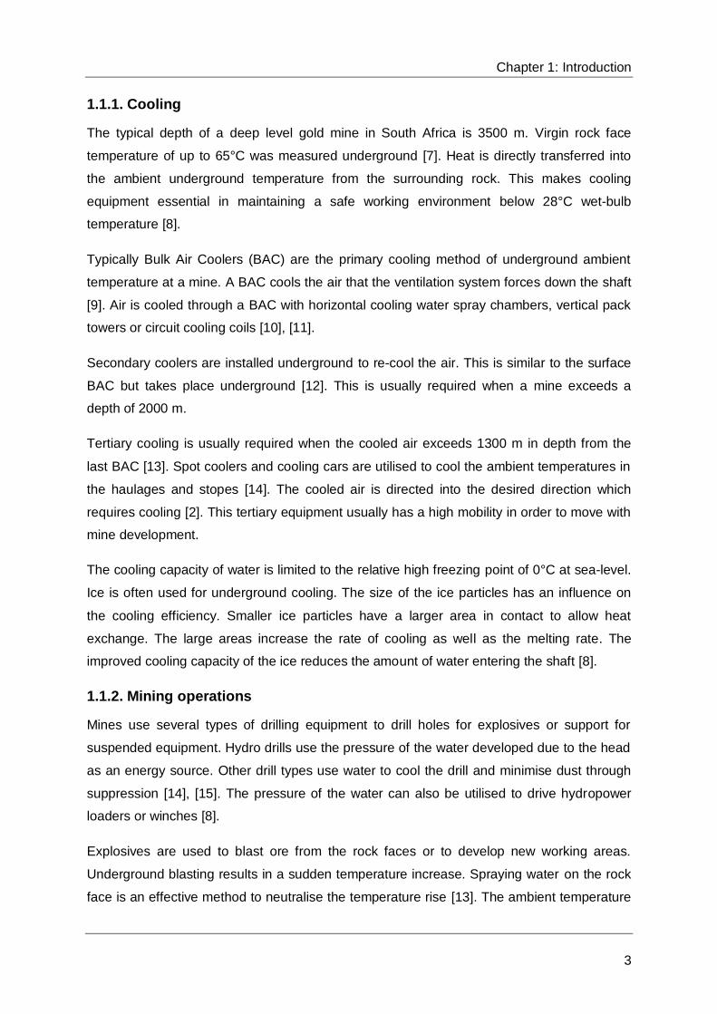
1.1.1. Cooling
The typical depth of a deep level gold mine in South Africa is 3500 m. Virgin rock face
temperature of up to 65°C was measured underground [7]. Heat is directly transferred into
the ambient underground temperature from the surrounding rock. This makes cooling
equipment essential in maintaining a safe working environment below 28°C wet-bulb
temperature [8].
Typically Bulk Air Coolers (BAC) are the primary cooling method of underground ambient
temperature at a mine. A BAC cools the air that the ventilation system forces down the shaft
[9]. Air is cooled through a BAC with horizontal cooling water spray chambers, vertical pack
towers or circuit cooling coils [10], [11].
Secondary coolers are installed underground to re-cool the air. This is similar to the surface
BAC but takes place underground [12]. This is usually required when a mine exceeds a
depth of 2000 m.
Tertiary cooling is usually required when the cooled air exceeds 1300 m in depth from the
last BAC [13]. Spot coolers and cooling cars are utilised to cool the ambient temperatures in
the haulages and stopes [14]. The cooled air is directed into the desired direction which
requires cooling [2]. This tertiary equipment usually has a high mobility in order to move with
mine development.
The cooling capacity of water is limited to the relative high freezing point of 0°C at sea-level.
Ice is often used for underground cooling. The size of the ice particles has an influence on
the cooling efficiency. Smaller ice particles have a larger area in contact to allow heat
exchange. The large areas increase the rate of cooling as well as the melting rate. The
improved cooling capacity of the ice reduces the amount of water entering the shaft [8].
1.1.2. Mining operations
Mines use several types of drilling equipment to drill holes for explosives or support for
suspended equipment. Hydro drills use the pressure of the water developed due to the head
as an energy source. Other drill types use water to cool the drill and minimise dust through
suppression [14], [15]. The pressure of the water can also be utilised to drive hydropower
loaders or winches [8].
Explosives are used to blast ore from the rock faces or to develop new working areas.
Underground blasting results in a sudden temperature increase. Spraying water on the rock
face is an effective method to neutralise the temperature rise [13]. The ambient temperature

Chapter 1: Introduction
4
must be maintained within mining regulations before the next shift can enter. The water
spray also acts as dust suppression for the dust released by the blasting [3].
The water pressure of the service water is used for cleaning and sweeping [8], [16]. A
flexible hose is installed to the service water column to improve manoeuvrability. Water-jet
nozzles installed on the flexible hoses increase the water velocity and concentrate the
direction of flow. This water has enough force to move the fine broken ore and dust [7].
Mines often utilise the used hot water to hoist ore. Crushers are installed underground to
obtain the desired ore particle size. The particles are dispensed in the used hot water to form
slurry. Positive displacement pumping systems are utilised to transfer the slurry. A positive
displacement pumping system can be in direct contact or isolated with a feeder or pressure
exchange system from the slurry [17].
1.2. Background to mine water reticulation systems
Mines use dewatering systems to remove the used service water, fissure and groundwater
from the shaft [14]. The used hot water is gravity fed to the settlers near shaft bottom
through the trenches from each level [18]. Settlers remove debris contaminating the water as
a result of mining activities. The clear hot water and mud water are then transferred to the
respective reservoirs [9], [19].
Lime flocculent is added to the contaminated water before it enters the settler. The flocculent
binds with the debris in the water to increase their density. The bonded debris then settles at
the bottom to allow separation from the clear hot water. The water must have a low pH of 8.5
for optimal performance of the process [9].
Mines often install a filter plant on the surface to remove the smaller particles from the water.
The settlers only remove larger particles to allow minimum damage to the dewatering
system. The most commonly found cooling system has small cavities through which the
water is transferred. The smallest particles will cause blockage, reducing the flow and
efficiency of the system.
The temperature of the hot water from underground is between 30 and 35°C [2]. Water with
a temperature of 3°C is required for effective cooling through the cooling equipment. A water
cooling system is installed to achieve the desired temperature.
The cleaned water is then transferred to pre-cool towers [7]. Pre-cool towers spray the water
to allow heat exchange with the atmosphere. Some pre-cool towers have fans to increase

Chapter 1: Introduction
5
the velocity of the air the water spray is in contact with to improve heat exchange efficiency.
The pre-cool towers lower the temperature of the water to approximately 8°C.
The pre-cool towers do not have enough cooling capacity to reduce the water temperature to
3°C in the summer. Refrigeration Plants (RP) proved to be the most efficient method to cool
the water [9]. RP operate on the vapour compressor refrigeration cycle. Refrigerant gas,
such as Freon or R-134a is compressed, condensed, expanded and evaporated. The
service water is cooled in a high pressure heat exchange vessel in the evaporator stage. A
closed water cycle is used for the condenser stage with cooling towers [2].
RP are usually located on the surface of a mine [4]. Some mines have installed secondary
underground RP. This reduces the load of the dewatering system, because not all the water
is pumped to the surface.
It is recommended, when optimising the pump schedule of the dewatering system, to
monitor the entire water reticulation system. This is especially important when the pressure
of the service water is harvested with a turbine or 3-CPFS. It ensures that all the dam levels
are controlled within acceptable limits for safe and sustainable mining [12].
Figure 2 displays a typical water reticulation system of a mine. The water cycles in a
clockwise manner. The pre-cool towers, refrigeration plants, refrigeration plant cooling
towers, settlers, hot water dams, mud reservoirs, slurry pumps and electrical pump chamber
often exist of multiple units. Only one unit is displayed in the figure.
1.3. Mine dewatering systems
Mines require water for multiple applications to enable safe and sustainable mining. This
water must also be removed from the shaft to prevent flooding. A dewatering system is
installed to remove water from underground. Dewatering systems were already utilised in
ancient Rome for underground operations [1].
Shaft dewatering is done in an upward cascading method to overcome the static head. The
water is pumped from the reservoir of the pump chamber near shaft bottom to a reservoir of
a higher pump chamber. This is repeated until the used hot water reaches the reservoir on
surface. The distance between two pump chambers can be up to 1380 m.

Chapter 1: Introduction
6
Figure 2: Typical water reticulation system of a mine
WATER TO
MINING
OPERATIONS
WATER FROM
MINING
OPERATIONS
ACTUATOR
CONTROLLED
VALVE
HOT WATER
DAM
ELECTRIC PUMP
CHAMBER
FILTER PLANT
TURBINE
POWERED
PUMP CHAMBER
SLURRY PUMP
CHAMBER
MUD
RESERVOIR
REFRIGIRATION
PLANT COOLING
WATER PIPE
COLD WATER
PIPE
HOT WATER
PIPE
CHILL WATER
PIPE
SLURRY WATER
PIPE
SLURRY DAM
REFIGITATION
PLANTS
REFRIGIRATION
PLANT COOLING
TOWER
BULK AIR
COOLER
SETTLER
FILTERED HOT
WATER PIPE
PRECOOLING
TOWER
3-CPFS
Chapter 1: Introduction
7
1.3.1. Pumps
Multistage centrifugal pumps are the preferred pumps to transfer fluid in many different
applications in the industrial and other sectors [1], [20], [21]. Multistage centrifugal pumps
are designed to tolerate more robust environments due to their flexibility and durability [22].
Newly developed multistage centrifugal pumps are designed for improved wear resistance,
increased availability and reduced maintenance cost. The designs also make maintenance
easier to decrease the period the pump is unavailable [1].
A single-stage centrifugal pump creates a discharge pressure by increasing the fluid velocity
through a rotating impeller [20]. A multistage centrifugal pump consists of multiple
successive single stages. The outlet of the first stage is guided directly to the inlet of the
second stage. Only the last stage has an outlet for the discharge flow.
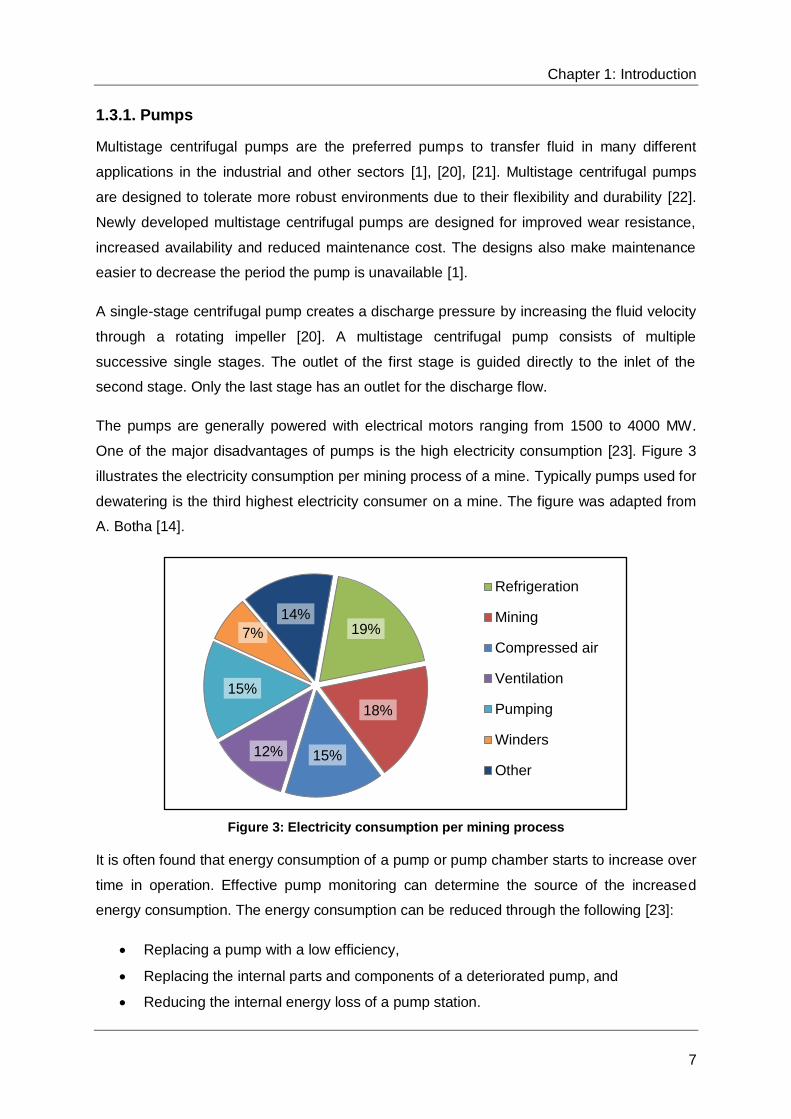
The pumps are generally powered with electrical motors ranging from 1500 to 4000 MW.
One of the major disadvantages of pumps is the high electricity consumption [23]. Figure 3
illustrates the electricity consumption per mining process of a mine. Typically pumps used for
dewatering is the third highest electricity consumer on a mine. The figure was adapted from
A. Botha [14].
Figure 3: Electricity consumption per mining process
It is often found that energy consumption of a pump or pump chamber starts to increase over
time in operation. Effective pump monitoring can determine the source of the increased
energy consumption. The energy consumption can be reduced through the following [23]:
Replacing a pump with a low efficiency,
Replacing the internal parts and components of a deteriorated pump, and
Reducing the internal energy loss of a pump station.
19%
18%
15%12%
15%
7%
14%
Refrigeration
Mining
Compressed air
Ventilation
Pumping
Winders
Other

Chapter 1: Introduction
8
Mines started to use alternative methods to dewater the shafts due to the high electricity
consumption of the pumps. The potential energy of the service water entering the shaft is
harvested through a hydropower turbine or a Three Chamber Pump Feeder System (3-
CPFS) [16]. Energy harvesting systems usually have a high initial infrastructure cost [24].
Both the systems must have a pump station and dissipater installed in parallel in case of
failure. The dissipater will also be used to meet the water demand if the system flow is
insufficient [25], [26].
1.3.2. Three chamber pump feeder system
A 3-CPFS harvests the potential energy of the service water entering the shaft to pump the
clear hot water [27]. The surface water has a high pressure due to the head of the water in
the columns. Installing a 3-CPFS can result in an electricity reduction of up to 80% [13].
The basic principle of a U-tube is applied on a 3-CPFS via a series of valves. One or multiple
booster pumps are installed to overcome the friction head in the columns. A PLC controls
the valves and pumps in sequence to ensure the potential energy if fully harvested [26].
Figure 4 is a basic diagram of a 3-CPFS.
a)
b)
Figure 4: Three chamber pump feeder system a) three stages and b) single stage
Table 1 explains the operation of one stage of a 3-CPFS [27]. The single stage in Figure 4 b
must be used with the explanation.
VALVE A
VALVE B
VALVE 1 VALVE 2
VALVE 3 VALVE 4
HIGH PRESSURE
CHILL WATERHIGH PRESSURE
HOT WATER
LOW PRESSURE
CHILL WATERLOW PRESSURE
HOT WATER

Chapter 1: Introduction
9
Table 1: Operation of a 3-CPFS
Step Action Result
1 Valves closed Chamber is filled with hot water with low pressure and no
flow.
2 Valve A opens Pressure inside the chamber equalises to the pressure of the
chill water.
3 Valves 1 and 2
open
The higher pressure of the chill water forces the hot water out
of the chamber.
4 Valves A,1 and 2
close
The chamber is filled with chill water with high pressure and
no flow.
5 Valve B opens Pressure inside the chamber decreases to less than the
pressure of the hot water at the inlet. This forms a vacuum
relative to the inlet hot water pressure.
6 Valves 3 and 4
open
The hot water fills the chamber due to the relative vacuum
formed. Chill water is sent down the shaft.
7 Valves B, 3 and 4
close
Low pressure inside the chamber with no flow similar to the
initial step. Step 2 to 7 is repeated during operation.
1.3.3. Hydropower turbines
Multiple shafts have installed turbines to harvest the potential energy of the service water.
The turbines are usually installed near a pumping chamber. Some shafts have multiple
turbines installed. The output shaft can either be coupled to a generator or a multistage
pump. The output power of a turbine can vary from 1 to 5 MW [7].
Pelton wheel turbines are the most efficient type of turbine. The typical efficiency of a turbine
installed in a mine ranges from 55 to 60%. Experimental Francis turbines installed were
found inadequate for this application [13].
A Pelton wheel turbine consists of a shaft, wheel, multiple buckets and water jet nozzles.
The buckets are installed on the periphery of the wheel. The buckets are shaped in the form
of spoons held together. The water jet nozzles increase the velocity of the water. The water
is directed at a tangent angle to the wheel onto the centre of the buckets where the two
spoons join. This causes a moment on the wheel which results in rotation of the shaft [28].
Figure 5 graphically shows the operation principle of a Pelton wheel turbine.

Chapter 1: Introduction
10
Figure 5: Operation of a Pelton wheel **1
Turbines are primarily used to harvest the potential energy of the service water entering the
shaft. The power generated from the turbines is often secondary applied to dewater the
shaft. The scheduling of the turbines should be included in the dewatering system.
1.4. Advantages of automation and control
The South African electricity supplier introduced a Time-of-Use (ToU) tariff structure for
industrial power consumers. The daily profile is divided into peak, standard and off-peak
periods. The periods are determined according to the electricity demand. The tariff is directly
influenced by the ToU. Other factors such as the distribution distance, voltage and season
also influence the cost. The 2014/2015 weekday winter cost tariff can be seen in Figure 6
[29].
Demand Side Management (DSM) projects were implemented according the ToU tariff
structure. The aim of DSM projects is to assist high electricity consumers to incentivise
electricity use in the lowest cost periods. This also reduces the electricity load on the grid of
South Africa. Typical DSM projects on high electricity consumers include the following [2]:
Load Shifting (LS) – Low to zero electricity load is consumed in the peak periods
through spreading the load into the other periods,
Peak Clipping (PC) – Reducing electricity load in the peak periods, and
Energy Efficiency (EE) – Daily electricity load is decreased.
** Some of the figures are for illustration purposes only and are not intended to represent state of the art technology. The reference for these figures will be footnoted. 1 Learn Easy. [Online]. Available: www.learneasy.info. [Accessed 30 July 2014].

Chapter 1: Introduction
11
Figure 6: Weekday Time-of-Use winter electricity tariff (2014/2015)
Dewatering systems have the potential to realise electricity cost saving through optimising
the control schedule according to the ToU tariff structure [30], [31]. This is achieved by
preparing dam levels to allow spare capacity to switch off pumps during the Eskom peak
periods [32]. Real-time monitoring to update the control schedule is required for LS [33].
The potential electricity savings of a dewatering system is determined through calculations,
measurement and verification and simulation [32]. A comparison of potential savings
achieved between manual and automated pump stations was done. It was determined that
manual pump control could achieve only 60% of the potential savings, whereas an
automated pump system could achieve up to 96%. Human intervention limits the savings
achieved [34].
It was proved that additional savings could be achieved if the pump load was minimised in
the standard periods. The pump load is shifted to the least expensive off-peak periods. The
correct starting and stopping time is crucial to realise additional savings. Pump automation is
recommended for real-time control [19].
The number of switches per pump has a direct impact on the maintenance frequency of a
pump. A pump experiences additional axial thrust until the impeller is balanced. The number
of stops and starts must be considered when optimising the control schedule [35], [32].
Automation of pumps allows for monitoring the number of switches and to prevent
unnecessary cycling.
0
50
100
150
200
250
00:0
0
01:0
0
02:0
0
03:0
0
04:0
0
05:0
0
06:0
0
07:0
0
08:0
0
09:0
0
10:0
0
11:0
0
12:0
0
13:0
0
14:0
0
15:0
0
16:0
0
17:0
0
18:0
0
19:0
0
20:0
0
21:0
0
22:0
0
23:0
0
Ele
ctr
icit
y c
os
t [
c/k
Wh
]
Time [hh:mm]
Off peak Peak Standard

Chapter 1: Introduction
12
Additional savings can be achieved by including the installed alternative dewatering systems
such as the turbines and 3-CPFS into the pump schedule. A mine shaft will achieve
maximum savings when the entire water reticulation system is automated. This includes the
BACs, FP, pre-cool towers, alternative dewatering systems, distribution of service water and
dewatering pumps. The systems can be interlocked to ensure safe and sustainable mining
when automated [36].
Workforce is often limited during the festive seasons or industrial action (also known as legal
strikes). Safe dewatering can be sustained during these periods if the pump system is
automated. Automation has the potential of labour cost savings. Less pump operators will be
required if a pump system is automated [1].
Pump monitoring is another advantage of pump automation. Instrumentation is required to
ensure safe remote operation. The performance and condition of each pump can be
determined from the data logged from the instrumentation [36]. Maintenance cost savings
can be achieved through correctly analysing the data.
1.5. Objectives and problem statement
Dewatering systems are crucial for sustainability in deep level mines. These systems are
being automated to reduce the amount of human intervention. Automation is achieved
through monitoring certain operating conditions. These conditions are then interlocked to
initiate an alarm or a stop sequence when it exceeds normal operating conditions.
The purpose of this study is to improve the current best practice of pump automation. This
will be achieved through investigating automated pump failure and detect the conditions
leading to failure. Reviewing the purpose of the installed instruments will make it possible to
identify the need for additional instrumentation or control alterations.
Remote control of the automated pumps can be achieved if they are connected to a data
network. The automated pump system makes it possible to control it from a centralised
system. This enables real-time control of the entire system. This is achieved through status
feedback over the network of all the individual control parameters.
This study will also verify the feasibility of controlling an automated mine dewatering system
from a surface control room. The control will focus on maintaining save operating dam levels
and electricity cost savings through minimising pumping in the peak periods.
Data from the conditions monitored of the automated pumps will be collected in real-time.
This is to limit the time the pump is operated at out of normal conditions. Access to the data
Chapter 1: Introduction
13
will make it possible to determine the most feasible method to calculate the real-time pump
efficiency.
The study will lastly use the installed instrumentation for automation and determine a method
to calculate the real-time efficiency. The method must exclude the pump flow. An accurate
flow meter is expensive and multiple pumps often use one column for dewatering.
1.6. Overview of dissertation
Chapter 1
This chapter explains deep level mine water consumption. An overview of a mine reticulation
system is given. It focuses on the different methods to dewater a deep level mine. This
chapter also lists the advantages of automating the dewatering system.
Chapter 2
The basic operating principle of a multi-stage centrifugal pump is explained. Understanding
the operating principle makes the investigation on the current best practice of automation
possible. Identifying and motivating the parameters to monitor with pump automation,
including auxiliaries. The characteristic and results of pump cavitation are discussed.
Chapter 3
A case study is presented of a pump that failed after it had been automated. The pump
failure was examined to determine the root cause of failure. Additional precautions and
safety measures are considered to prevent a similar incident. The control philosophies for a
dewatering system are discussed. An alternative method to determine pump efficiency in
real-time is implemented.
Chapter 4
The results of the installed instrumentation of a pump are shown. The additional precautions
and safety measures are verified to determine if it will prevent a similar incident. Pump
running statuses are discussed with the implemented control philosophies. The real-time
efficiencies of the pumps calculated are shown.
Chapter 5
A conclusion based on the results obtained is made. The results also make it possible to
suggest alterations to the project. From this study several opportunities for further studies
were identified. These opportunities are also discussed in this chapter.

14
Chapter 2: Pump automation overview
Understanding the operating principle of a multi-stage centrifugal pump is necessary to
improve the automation of the system. The current best practice to automate a multi-stage
centrifugal pump is investigated. This assists in motivating the conditions that should be
monitored when automating pump system.

Chapter 2: Pump automation overview
15
2.1. Introduction
Automation of a pump or pump station has multiple potential advantages. Several
parameters should be investigated when automating a pump. This ensures the best possible
solution is installed. The parameters that must be investigated will be discussed in this
chapter.
Included in pump automation is pump monitoring. This allows for safe remote start or stop
without direct human intervention. The differences between condition and performance
monitoring will be compared. Critical conditions and deliverables that should be included in
the pump automation to ensure optimal pump operation will be investigated.
All the necessary auxiliaries of a pump should be considered and automated when a pump
is automated. The discharge valve is one of the key auxiliaries to automate within the pump
system. The different types of valves often used as discharge valves are discussed. Several
methods to automate the discharge valve are also included in this chapter.
Pump cavitation is known as a destructive condition that results in pump failure. The origin of
cavitation is discussed and methods included in pump automation specified by
manufacturers are investigated. The effect of cavitation on the hydrodynamic performance of
a pump is also determined.
2.2. Multi-stage centrifugal pumps
The expected lifetime of a multistage centrifugal pump is 15 years. The regular life of a pump
can be increased with up to 15% if the correct maintenance is done. This can reduce the
energy consumed with up to 7% [1]. The lifetime reduces when the pump operates outside
the design conditions. Maintenance frequency should be increased if the fluid transferred
has corrosive properties [22].
Refurbishing a pump is not feasible if the cost exceeds 40% of the price of a new pump.
Refurbishing or upgrading a pump typically involves internal renovation, modernization of the
seal system and a revamp of the lubrication oil system. Pump system upgrades include
increasing the rating of the pump power source, pump re-wheeling, control valve
modification and various piping changes [37].
A pump should be investigated for refurbishment if the power consumption increases with a
constant discharge flow. The increased power consumption is an indication of a decreasing
efficiency. A decreased efficiency implies that the pump must pump for a longer period to

Chapter 2: Pump automation overview
16
transfer the same amount of fluid. Condition monitoring and performance monitoring of the
pump can assist with the decision on when to refurbish the pump [38].
Upgrading the motor or the impeller can result in an energy saving of up to 3.5%. When a
pump is upgraded as a unit, including electrical equipment and motor pump, the saving can
improve with up to 10%. If the pump system is examined as a system, including pumps,
piping, control and operating strategies, a saving of up to 60% is achievable [33].
A breakdown of the total cost of a typical multistage centrifugal pump during its operation
cycle is illustrated in Figure 7 [33], [22]. At 40%, power consumption is the largest expense
of a pump during its operation cycle. Maintenance contributes to 25% of the total cost of a
pump. Installing effective pump monitoring equipment to improve pump reliability can result
in power consumption and maintenance cost saving [39].
Figure 7: Breakdown of total cost of a pump during its lifetime
2.2.1. Failures
Failure of pumps is a concern for any pumping station. It can result in the pump system not
meeting the demand when no spare capacity is available. This increases the risk of flooding
a mine. The following list is the main reasons for pump failure [40]:
Design, fabrication and assembly faults,
Incorrect installation or commissioning,
Change in operating conditions, and
Mechanical wear from operation.
Pumps are designed with little clearance tolerances to achieve the highest efficiency
possible. This reduces the out of design operation margin [41]. Fabrication and assembly of
15%
10%
40%
25%
10%Purchase
Installation
Energy
Maintenance
Operating

Chapter 2: Pump automation overview
17
a pump are of utmost importance due to small tolerances. A pump will experience additional
internal stresses and vibration, which can result in failure [42], [43].
Correct installation and commissioning of a pump are important to ensure all safeties and
trips are operational [41]. A condition monitoring or safety circuit is only as effective as the
least trustworthy data collected from the pump. If the data is unreliable or corrupt, the
condition monitoring will not be as effective [33], [43].
A change in operating condition can result in transient flow. During transient flow, the
equipment is subject to rapid temperature, pressure and speed changes. In most cases of
transient flow the conditions exceeds the design condition [40], [42].
The most common incorrect operations of centrifugal pumps that lead to failure are [44]:
Insufficient suction pressure leading to cavitation,
Excessively high flow rate for the Net Positive Suction Head available (NPSHa),
Prolonged operation at lower than acceptable flow rates,
Operation of the pump at zero or near zero flow rate,
Improper operation of pumps in parallel,
Failure to maintain adequate bearing lubrication, and
Failure to maintain satisfactory flushing of mechanical seals.
Knowledge and experience obtained can assist on determination of failure through visual
inspection. It is recommended for confirmation of failure to be revealed from metallurgical
laboratory tests [45].
2.2.2. Head required
The head required in a pumping system is the static head plus the friction head. The static
height is the difference in height between the fluid surface the reservoir pumping from, to the
highest point of travel of the fluid [46]. The friction head is the differential pressure of the fluid
through the component used to transport the fluid [47].
Experimental results define loss coefficients for each component. The friction head is due to
velocity change, direction changes or flow restriction. Friction head is calculated with
Equation 2.1 from the loss coefficient [48].

Chapter 2: Pump automation overview
18
2.1.
- Component friction head m
- Loss coefficient -
- Fluid velocity m/s
- Gravitational Constant m/s2
Valves are used to control flow in a pumping system. A valve that is fully closed will have an
infinite loss coefficient to produce zero head at the outlet. The total friction head of a system
containing more than one component is the sum of the losses. The loss coefficients of the
following components are usually considered within a pumping system:
Suction and discharge nozzles,
Inline pipe diameter variations,
Valves and flow restrictions, and
Elbows, bends and tees.
The flow of fluid through a pipe causes friction that results in an additional friction head. The
friction is a function of the type of flow and internal smoothness of the pipe. The friction head
due to the friction is calculated with Equation 2.2 [49].
2.2.
- Pipe friction head m
- Friction coefficient of pipe -
- Length of pipe m
- Fluid velocity m/s
- Inside diameter of pipe m
- Gravitational Constant m/s2
The total head required by a pump is illustrated with Figure 8. The water is pumped from
reservoir A to reservoir B. The differential height difference between the water surface A and
the highest point of travel is defined as .
More pumps are often specified and installed than required when designing a pumping
station. This allows one or more pumps to be on standby in case of an emergency. It is
frequently found that design parameters are neglected and all the pumps are operated
simultaneously [50].

Chapter 2: Pump automation overview
19
The efficiency of the pumping system decreases if the number of pumps operated
simultaneously increases and discharges into one column. The increased flow through pipes
and pipeline components increases friction losses. The total energy to transfer the same
amount of water increases due to deteriorated efficiency. Controlling according the design
will reduce the energy consumed and maintenance cost [50].
Figure 8: Pumping system total head required
The friction head due to the suction and discharge nozzle is defined as and
respectively. The friction caused by the pipe from the suction to pump inlet is defined as
. The valve and NRV on the pump outlet causes a friction head defined respectively as
and . The friction head from the valve to the discharge is defined as . There is a
total of eight identical elbows in the system that individually causes a friction head defined as
. The total head required by the pump is calculated with Equation 2.3 [46].
2.3.
- Head m
- Static head m
- Suction nozzle friction head m
- Suction pipe friction head m
- Valve friction head m
- NRV friction head m
- Discharge pipe friction head m
- Discharge nozzle friction head m
- Pipe elbow friction head m
RESERVOIR B
RESERVOIR A
Vh
NRVh
vhelbh
elbh
elbhelbh
elbh
elbh
elbh
SH
snh
dnh
elbh
fsph
fdph

Chapter 2: Pump automation overview
20
The total head developed is the sum of differential energy across the pump. The differential
energy consists of the potential and kinetic energy from the pump inlet to the pump outlet.
Equation 2.4 illustrates how to calculate the head that a pump develops [51].
(
)
2.4.
- Head m
- Outlet pressure Pa
- Inlet pressure Pa
- Outlet height M
- Inlet height m
- Outlet velocity m/s
- Inlet velocity m/s
- Fluid density kg/m3
- Gravitational Constant m/s2
The velocity of the fluid has a direct impact on the friction head of a system. Pumps in a
pump system are often installed in parallel. The velocity of the fluid is increased if more than
one pump transfers fluid in a single discharge column. The increased velocity increases the
friction head of the system [23]. The increased pressure also adds risk of column failure.
2.3. Current best practices to automate a pump
It is desired to operate pumps at their maximum efficiency, reliability, capacity and minimum
operating and maintenance cost. This will reduce the total running cost of the pumping
station [40]. Pump monitoring is included in the current best practice when automating a
pump. Pump monitoring promotes preventative maintenance to predictive maintenance. This
results in only necessary components being replaced, instead of changing certain
components after a set time period [40], [52].
Effective pump monitoring can improve pump reliability through root-cause failure analysis. It
can identify a condition at an early stage that could lead to pump damage. This reduces the
risk of unpredictable failure and down time [40], [42]. Replacing or repairing the weakening
component before failure can also enhance the performance of the pump [42], [52].
Multiple instruments are installed on a pump to monitor several conditions and deliverables.
Proven reliable instrumentation should be installed for pump monitoring. The feedback
received from instrumentation should be interlocked in a control program. The functionality
and failure probability of a component should be taken into consideration when designing a
pump monitoring system [53].

Chapter 2: Pump automation overview
21
The normal condition and deliverables of a new pump should be logged before wear or
damage occurs as a reference point. Operating ranges of the pump of healthy operation
should be defined and logged [40], [52]. An alarm must be activated if the defined limit is
reached, determined from the healthy operation data. If the condition continues to exceed
healthy conditions, an emergency shutdown must be initiated [40], [42].
Modern pump systems must be seen as an integrated operation including the hardware,
software, operating procedures, control philosophies and process condition. Pump
monitoring is included in the system to increase the availability of a pump [53]. All
components of an individual pump, including the motor, transmission, pump, auxiliaries,
valves, lubrication and seal system must be monitored continuously [42].
Pump monitoring can be divided into two groups, namely performance monitoring and
condition monitoring. Performance monitoring determines the efficiency of a pump with the
deliverable. Condition monitoring reduces the risk of failure. Performance monitoring does
not replace condition monitoring. It assists with the analysis of the condition monitoring data.
[54]. Figure 9 shows the different parameters and benefits [54].
Figure 9: Pump condition and performance monitoring
Performance Monitoring
Flow
Pressure
Power
Condition Monitoring
Vibration
Temperature
Operating Functions
Pump performance cost
Energy cost
Optimisation of performance
Economic refurbishment
Economic replacement
Asset management
Maintenance Function
Preventative maintenance
Failure analysis
Chapter 2: Pump automation overview
22
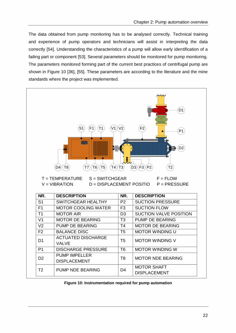
The data obtained from pump monitoring has to be analysed correctly. Technical training
and experience of pump operators and technicians will assist in interpreting the data
correctly [54]. Understanding the characteristics of a pump will allow early identification of a
failing part or component [53]. Several parameters should be monitored for pump monitoring.
The parameters monitored forming part of the current best practices of centrifugal pump are
shown in Figure 10 [36], [55]. These parameters are according to the literature and the mine
standards where the project was implemented.
T = TEMPERATURE S = SWITCHGEAR F = FLOW
V = VIBRATION D = DISPLACEMENT POSITIO P = PRESSURE
NR. DESCRIPTION NR. DESCRIPTION
S1 SWITCHGEAR HEALTHY P2 SUCTION PRESSURE
F1 MOTOR COOLING WATER F3 SUCTION FLOW
T1 MOTOR AIR D3 SUCTION VALVE POSITION
V1 MOTOR DE BEARING T3 PUMP DE BEARING
V2 PUMP DE BEARING T4 MOTOR DE BEARING
F2 BALANCE DISC T5 MOTOR WINDING U
D1 ACTUATED DISCHARGE
VALVE T5 MOTOR WINDING V
P1 DISCHARGE PRESSURE T6 MOTOR WINDING W
D2 PUMP IMPELLER
DISPLACEMENT T8 MOTOR NDE BEARING
T2 PUMP NDE BEARING D4 MOTOR SHAFT
DISPLACEMENT
Figure 10: Instrumentation required for pump automation
T7 T6 T5 T3 T2F3T8D4 T4 D3 P2
V2 F2
D2
P1
D1
T1F1 V1S1

Chapter 2: Pump automation overview
23
Flow
The flow of a pump must be included in pump monitoring. Worn internal parts can be
detected if the rated design flow from the manufacturer is not delivered at a specific speed
[42], [56]. A pump can be damaged if the flow through a pump is less than the design
minimum. Installing flow sensors will prevent the pump against minimum flow [38].
Pumps should be started at the nearly closed discharge valve position. The pump generates
head as the discharge valve opens to overcome the pressure in the discharge column. For
minimum flow restriction the suction and discharge valves should be opened fully when the
start-up sequence has been completed [57].
It is often found that the discharge valve of a pump is throttled to regulate the flow of the
pump [52]. Additional wear occurs on the internal components if the discharge valve is
throttled. This increases the maintenance cost and frequency of a pump [47].
Balance disc flow monitoring is recommended [38]. The balance disc flow acts as a thrust
bearing for the pump to counteract the axial force of the impeller. The water is pumped
between the balance disc and the balancing chamber, creating a thin film layer water
bearing [52].
Pressure
The pump columns are often undersized, both in design and due to inconsistent
maintenance frequencies [23]. When a pump starts with low flow against a barely open
discharge valve, the pressure will be greater than normal operating pressures. The
discharge column from the pump outlet to the discharge valve should be designed to endure
the higher pressures during start-up [57].
The water level inside the discharge column is determined with pressure sensors. A pump
must always be started with a full discharge column. If the column is drained, the column
must be filled before the pump can be started. The safety trip circuit of the pump during start-
up should include the water pressure of the discharge column.

Chapter 2: Pump automation overview
24
Power
It is recommended to install a Variable Speed Drive (VSD) to control the flow of a pump. A
VSD alters the current frequency and voltage frequency of the motor to adjust the rotational
speed accordingly [20]. Reducing the motor frequencies of a pump via a VSD also has an
energy-saving potential [23].
Using a VSD ensures the rotational velocity is gradually increased to operating speed when
starting and gradually decreased when stopped, resulting in less mechanical strain induced
on the pump from the moment of inertia. This reduces the maintenance frequency of a pump
and motor [47].
An increase in power consumption on a pump that is controlled on the discharge pressure or
flow via a VSD can be an indication of a worn impeller. The rotational velocity of the pump
has to be increased to meet the demand of the system. A high power alarm will alert the
pump operators of the additional power consumption [56]. A pump dewatering system
requires a constant head at full load power. VSD’s are not installed on the pump dewatering
systems.
During pump start-up, for a brief period, the power consumed is higher than the operating
power. This is a result of system friction and moment of inertia. The additional system friction
during start-up includes the discharge head, barely open discharge valve, non-return valve
not opening or transient flow through the pump [6]. The real-time motor power can indicate
whether the pump is operated incorrectly.
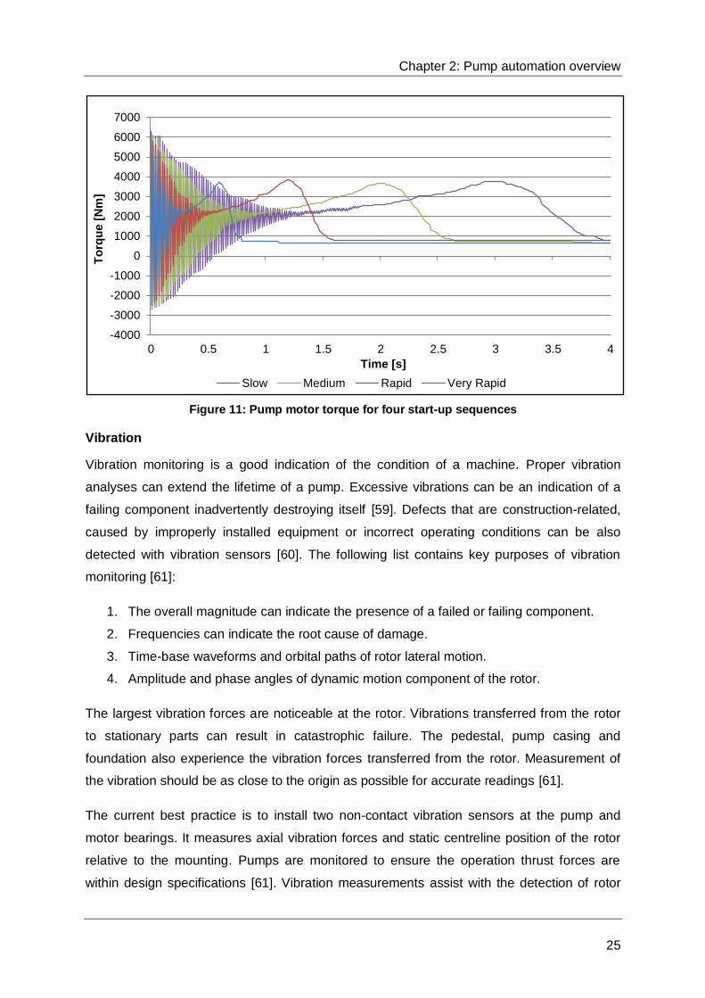
The torque required for four different starting speeds are displayed in Figure 4. It can be
seen that the basic profiles of the graphs are similar. The period of fluctuation during start-up
is directly proportional to the start-up speed. The fluctuation is a result of system friction and
moment of inertia.
The fluctuation for all four speeds settles at approximately 2300 Nm. The torque increases to
a maximum of 3600 Nm from where the torque decreases to operating torque. The operating
torque is required to account for the pump and motor friction forces. The graph is a
combination of the graphs found in S Elaoud and E Hadj-Taïeb [58]. The original graphs are
shown in Appendix A.
Chapter 2: Pump automation overview
25
Figure 11: Pump motor torque for four start-up sequences
Vibration
Vibration monitoring is a good indication of the condition of a machine. Proper vibration
analyses can extend the lifetime of a pump. Excessive vibrations can be an indication of a
failing component inadvertently destroying itself [59]. Defects that are construction-related,
caused by improperly installed equipment or incorrect operating conditions can be also
detected with vibration sensors [60]. The following list contains key purposes of vibration
monitoring [61]:
1. The overall magnitude can indicate the presence of a failed or failing component.
2. Frequencies can indicate the root cause of damage.
3. Time-base waveforms and orbital paths of rotor lateral motion.
4. Amplitude and phase angles of dynamic motion component of the rotor.
The largest vibration forces are noticeable at the rotor. Vibrations transferred from the rotor
to stationary parts can result in catastrophic failure. The pedestal, pump casing and
foundation also experience the vibration forces transferred from the rotor. Measurement of
the vibration should be as close to the origin as possible for accurate readings [61].
The current best practice is to install two non-contact vibration sensors at the pump and
motor bearings. It measures axial vibration forces and static centreline position of the rotor
relative to the mounting. Pumps are monitored to ensure the operation thrust forces are
within design specifications [61]. Vibration measurements assist with the detection of rotor
-4000
-3000
-2000
-1000
0
1000
2000
3000
4000
5000
6000
7000
0 0.5 1 1.5 2 2.5 3 3.5 4
To
rqu
e [
Nm
]
Time [s]
Slow Medium Rapid Very Rapid

Chapter 2: Pump automation overview
26
vibration. The natural frequency for most pumps in the tangent direction is higher than in the
axial direction [62].
A vibration sensor installed on the casing, inlet or outlet column of a pump, measures the
vibration of the fluid. Fluid vibrations are an indication of the fluid energy. Transient flow and
cavitation can be detected from measuring fluid vibration [59]. It must be noted that casing
vibration measurement does not measure shaft vibration.
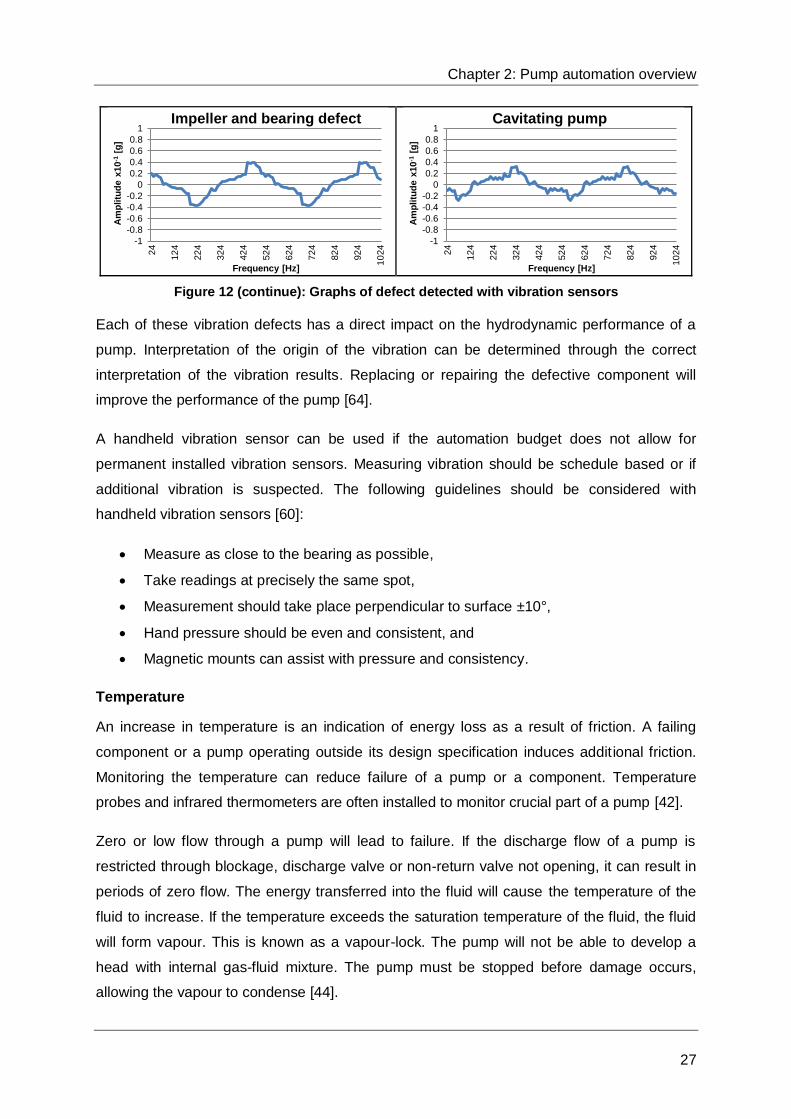
Plotting the results of a vibration sensor can indicate multiple defects and operating errors of
a pump. Figure 12 illustrates the difference between the graphs of a pump with various
defects or operating errors. The graphs are simplified from N R Sakthivel et el. [63]. The
original graphs can be found in Appendix A.
It can be seen that a pump with a bearing defect will have the maximum amplitude of
vibration of the primary sine wave. A pump with only a seal defect reduces the amplitude of
vibration of the primary sine wave. The other defects only change the frequency of the
secondary sinus wave. Experience in the field of vibration analysis will enable a person to
identify the different defects from vibration graphs.
Figure 12: Graphs of defects detected with vibration sensors
-1
-0.8
-0.6
-0.4
-0.2
0
0.2
0.4
0.6
0.8
1
24
12
4
22
4
32
4
42
4
52
4
62
4
72
4
82
4
92
4
10
24
Am
plitu
de x
10
-1[g
]
Frequency [Hz]
Normal operating pump
-1
-0.8
-0.6
-0.4
-0.2
0
0.2
0.4
0.6
0.8
1
24
12
4
22
4
32
4
42
4
52
4
62
4
72
4
82
4
92
4
10
24
Am
plitu
de x
10
-1[g
]
Frequency [Hz]
Impeller defect
-1
-0.8
-0.6
-0.4
-0.2
0
0.2
0.4
0.6
0.8
1
24
12
4
22
4
32
4
42
4
52
4
62
4
72
4
82
4
92
4
10
24
Am
plitu
de x
10
-1[g
]
Frequency [Hz]
Bearing defect
-1
-0.8
-0.6
-0.4
-0.2
0
0.2
0.4
0.6
0.8
1
24
12
4
22
4
32
4
42
4
52
4
62
4
72
4
82
4
92
4
10
24
Am
plitu
de x
10
-1[g
]
Frequency [Hz]
Seal defect
Chapter 2: Pump automation overview
27
Figure 12 (continue): Graphs of defect detected with vibration sensors
Each of these vibration defects has a direct impact on the hydrodynamic performance of a
pump. Interpretation of the origin of the vibration can be determined through the correct
interpretation of the vibration results. Replacing or repairing the defective component will
improve the performance of the pump [64].
A handheld vibration sensor can be used if the automation budget does not allow for
permanent installed vibration sensors. Measuring vibration should be schedule based or if
additional vibration is suspected. The following guidelines should be considered with
handheld vibration sensors [60]:
Measure as close to the bearing as possible,
Take readings at precisely the same spot,
Measurement should take place perpendicular to surface ±10°,
Hand pressure should be even and consistent, and
Magnetic mounts can assist with pressure and consistency.
Temperature
An increase in temperature is an indication of energy loss as a result of friction. A failing
component or a pump operating outside its design specification induces additional friction.
Monitoring the temperature can reduce failure of a pump or a component. Temperature
probes and infrared thermometers are often installed to monitor crucial part of a pump [42].
Zero or low flow through a pump will lead to failure. If the discharge flow of a pump is
restricted through blockage, discharge valve or non-return valve not opening, it can result in
periods of zero flow. The energy transferred into the fluid will cause the temperature of the
fluid to increase. If the temperature exceeds the saturation temperature of the fluid, the fluid
will form vapour. This is known as a vapour-lock. The pump will not be able to develop a
head with internal gas-fluid mixture. The pump must be stopped before damage occurs,
allowing the vapour to condense [44].
-1
-0.8
-0.6
-0.4
-0.2
0
0.2
0.4
0.6
0.8
1
24
12
4
22
4
32
4
42
4
52
4
62
4
72
4
82
4
92
4
10
24
Am
plitu
de x
10
-1[g
]
Frequency [Hz]
Impeller and bearing defect
-1
-0.8
-0.6
-0.4
-0.2
0
0.2
0.4
0.6
0.8
1
24
12
4
22
4
32
4
42
4
52
4
62
4
72
4
82
4
92
4
10
24
Am
plitu
de x
10
-1[g
]
Frequency [Hz]
Cavitating pump
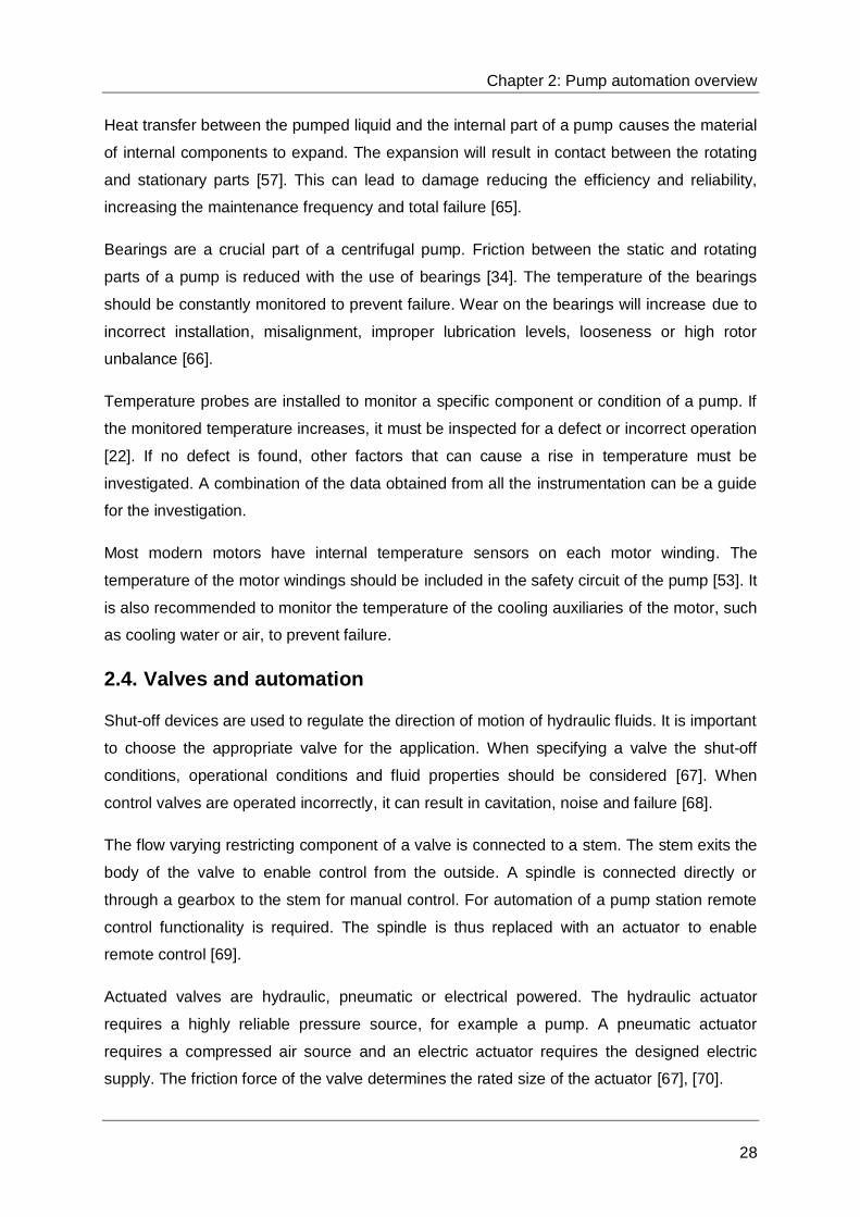
Chapter 2: Pump automation overview
28
Heat transfer between the pumped liquid and the internal part of a pump causes the material
of internal components to expand. The expansion will result in contact between the rotating
and stationary parts [57]. This can lead to damage reducing the efficiency and reliability,
increasing the maintenance frequency and total failure [65].
Bearings are a crucial part of a centrifugal pump. Friction between the static and rotating
parts of a pump is reduced with the use of bearings [34]. The temperature of the bearings
should be constantly monitored to prevent failure. Wear on the bearings will increase due to
incorrect installation, misalignment, improper lubrication levels, looseness or high rotor
unbalance [66].
Temperature probes are installed to monitor a specific component or condition of a pump. If
the monitored temperature increases, it must be inspected for a defect or incorrect operation
[22]. If no defect is found, other factors that can cause a rise in temperature must be
investigated. A combination of the data obtained from all the instrumentation can be a guide
for the investigation.
Most modern motors have internal temperature sensors on each motor winding. The
temperature of the motor windings should be included in the safety circuit of the pump [53]. It
is also recommended to monitor the temperature of the cooling auxiliaries of the motor, such
as cooling water or air, to prevent failure.
2.4. Valves and automation
Shut-off devices are used to regulate the direction of motion of hydraulic fluids. It is important
to choose the appropriate valve for the application. When specifying a valve the shut-off
conditions, operational conditions and fluid properties should be considered [67]. When
control valves are operated incorrectly, it can result in cavitation, noise and failure [68].
The flow varying restricting component of a valve is connected to a stem. The stem exits the
body of the valve to enable control from the outside. A spindle is connected directly or
through a gearbox to the stem for manual control. For automation of a pump station remote
control functionality is required. The spindle is thus replaced with an actuator to enable
remote control [69].
Actuated valves are hydraulic, pneumatic or electrical powered. The hydraulic actuator
requires a highly reliable pressure source, for example a pump. A pneumatic actuator
requires a compressed air source and an electric actuator requires the designed electric
supply. The friction force of the valve determines the rated size of the actuator [67], [70].
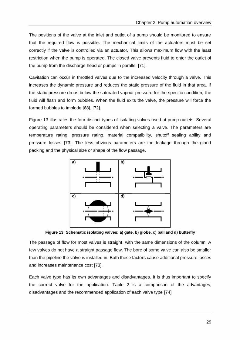
Chapter 2: Pump automation overview
29
The positions of the valve at the inlet and outlet of a pump should be monitored to ensure
that the required flow is possible. The mechanical limits of the actuators must be set
correctly if the valve is controlled via an actuator. This allows maximum flow with the least
restriction when the pump is operated. The closed valve prevents fluid to enter the outlet of
the pump from the discharge head or pumps in parallel [71].
Cavitation can occur in throttled valves due to the increased velocity through a valve. This
increases the dynamic pressure and reduces the static pressure of the fluid in that area. If
the static pressure drops below the saturated vapour pressure for the specific condition, the
fluid will flash and form bubbles. When the fluid exits the valve, the pressure will force the
formed bubbles to implode [68], [72].
Figure 13 illustrates the four distinct types of isolating valves used at pump outlets. Several
operating parameters should be considered when selecting a valve. The parameters are
temperature rating, pressure rating, material compatibility, shutoff sealing ability and
pressure losses [73]. The less obvious parameters are the leakage through the gland
packing and the physical size or shape of the flow passage.
a)
b)
c)
d)
Figure 13: Schematic isolating valves: a) gate, b) globe, c) ball and d) butterfly
The passage of flow for most valves is straight, with the same dimensions of the column. A
few valves do not have a straight passage flow. The bore of some valve can also be smaller
than the pipeline the valve is installed in. Both these factors cause additional pressure losses
and increases maintenance cost [73].
Each valve type has its own advantages and disadvantages. It is thus important to specify
the correct valve for the application. Table 2 is a comparison of the advantages,
disadvantages and the recommended application of each valve type [74].

Chapter 2: Pump automation overview
30
Table 2: Valve type comparison
Valve Gate Ball Globe Butterfly
Type Open/Close Open/Close Throttling Throttling
Ad
va
nta
ge
s
Minimal pressure
loss across valve
Low flow
restriction induced
with debris
Minimal pressure
loss across valve
Low flow
restriction induced
with debris
Compact design
High capacity
Good shut-off
Good shut-off
High opening and
closing frequency
Inline replacement
of trim
High capacity
Noise reduction
cage available
Smooth control
Compact design
Minimal pressure
loss across valve
Low cost
High throughput
capacity
Smaller shaft and
actuator
Dis
ad
van
tage
s
Poor sealing
characteristic
Valve must be
removed for
maintenance
Temperature
range limited due
to seats
High flow
restriction
Cavitation
Valve must be
removed for
maintenance
High pressure loss
due to tortuous
flow path
Noise reduction
cage reduces
capacity
Poor sealing
characteristics
Efficient control
limited to 60° open
Specialized lining,
oversized shaft
and actuator are
required for tight
shut-off
Re
co
mm
en
de
d
app
lica
tion
s
Not for frequent
opening or closing
Throttled control is
not recommended
Not for service
with highly
corrosive fluids
Most suitable for
handling slurries
Flow regulation
Tight shut-off
applications
Low-pressure
applications
Valves that use a spindle to control the position of the flow restriction body have glands to
seal the valve. The type of gland is dependent upon the fluid properties. The seals may
require a liquid quench, a piped vent, or a gas blanket. Incorrectly specified glands will cause
early leakages which can increase the maintenance intervals [73].
It is often found that maintenance on valves is based on a time schedule. Installing condition
monitoring equipment on these valves can detect if a valve is not operating correctly. This
can reduce the maintenance frequency on the valves [68].

Chapter 2: Pump automation overview
31
Valves often deteriorate more rapidly if used in a corrosive medium and significant
temperature gradients. Wear to the internal components, connections and welds is often
found on shut-off devices [75]. It is often difficult to open a valve if a large differential
pressure is present across the valve [57], [73]. The differential pressure induces additional
friction in a valve.
The discharge valve of a pump can induce water hammer during start up or shut down of a
pump. The control of an actuated valve should be programmed correctly to prevent water
hammer [76]. The response of the discharge valve actuator is not directly proportional to the
control signal [20].
2.4.1. Gate valves
A gate valve has a straight flow passage through the valve. The valve has a disc, known as
the gate or knife, to restrict the flow. The gate moves perpendicularly to the flow to open or
close the valve [69]. The valve has a bonnet area to house the gate when fully open. The
gate is attached to a stem with square screw thread to control the position of the gate. Figure
14 displays a sectional view of a gate valve.
A gate valve is often used as shut-off devices for large diameter pipes with high pressure. A
gate valve is highly reliable, especially when operating in a medium containing abrasive
particles [56], [67].
Figure 14: Sectional view of a gate valve 2
2 Trade India. [Online]. Available: www.tradeindia.com. [Accessed 04 June 2014].

Chapter 2: Pump automation overview
32
2.4.2. Globe valves
A globe valve consists of a plug-type disc seated against a port. The port is perpendicular to
the inlet and outlet flanges to enable the plug to restrict the flow. This flow path is known as
a tortuous flow path [77]. The flow is forced upward through the port to the outlet [69]. Figure
15 displays a sectional view of a globe valve.
Figure 15: Sectional view of a globe valve3
Globe valves are commonly used in pipelines that transfer fluid which contains pulverised
solids. In this regard it was found that the current globe valve design had multiple
disadvantages. The pulverised solid in the fluid damages the internal components of the
valve. This results in wear of the airproof components and dramatically shortens the lifetime
of the valve [78].
Cage-style trims were designed to prevent cavitation in globe valves. The cages are
designed to regulate the flow evenly through the valves. Prior to the trim a downstream
orifice was installed inline to protect the valve against cavitation. This results in only moving
the cavitation to the orifice instead of inside the valve [39].
2.4.3. Ball valves
A ball valve has a ball in line with the flow passage. The ball has a straight bore hole to allow
flow through the valve. The ball rotates from parallel to perpendicular with reference to the
inlet and outlet. When the ball is rotated to its maximum position, the flow is shut-off [79].
3 Weir. [Online]. Available: www.weirpowerindustrial.com. [Accessed 04 June 2014].

Chapter 2: Pump automation overview
33
Figure 16: Sectional view of a ball valve4
2.4.4. Butterfly valves
The flow follows a straight passage through a butterfly valve. The valve consists of an in-line
disc that rotates from parallel to perpendicular with reference to the inlet and outlet [69]. A
pressure loss is present even when the butterfly valve is fully open due to presence of the
disc in the flow path [80]. Figure 17 is an isometric view of a butterfly valve.
Figure 17: Isometric view of a butterfly valve5
A butterfly valve is often used to control the flow of gas, oil, water or air in large transport
systems. The typical operating range of a butterfly valve is between 30% and 70% open. If
the opening exceeds 70%, the pressure loss is almost constant [81]. Butterfly valves require
more torque to operate than the other valves due to the torque induced by the liquid on the
disc [70].
4 Global valve & Controls. [Online]. Available: www.globalvalveandcontrols.com. [Accessed 21 June
2014]. 5 Weir. [Online]. Available: www.weirpowerindustrial.com. [Accessed 04 June 2014].

Chapter 2: Pump automation overview
34
2.4.5. Non-return valve
Pumps that operate against a high head or in parallel should have a Non-Return Valve
(NRV) installed in-line on the discharge column. This acts as a mechanical safety if the
controlled discharge valve fails. The NRV will prevent the pressure in the discharge column
to rotate the pump backward [57], [58].
Figure 18 displays two types of NRV. Valve a in Figure 18 is known as a piston type NRV. It
operates on the same principle as a globe valve. The main difference is the plug is spring-
loaded instead of attached to a stem. Adjusting the stiffness of the spring will determine the
pressure at which the valve will allow flow through.
Valve b in Figure 18 is known as a swing type NRV. It has a disc that pivots on a hinge. As
soon as the inlet pressure is higher than the outlet, the disc will open. The outlet pressure
and gravitational force ensure that the valve closes. The body of the valve prevents the disc
to pivot past the closed position.
a)
b)
Figure 18: Sectional view of NRV: a) piston type; and b) swing type6
2.5. Characteristics of pump cavitation
Pump cavitation occurs when the static pressure within the pump drops below the saturated
vapour pressure of the specific fluid. The saturated vapour pressure depends on the
properties of the fluid. When the static pressure drops below saturation vapour pressure, the
fluid flashes and vaporisation occurs. The bubbles formed flow to the higher discharge
pressure where the bubbles collapse and condense [82].
The collapsing bubbles release a sudden energy force inside the pump. This energy
damages the internal components of a pump [59]. Damaged caused by these collapsing
6 Explore the World of Piping. [Online]. Available: www.wermac.org. [Accessed 04 June 2014].
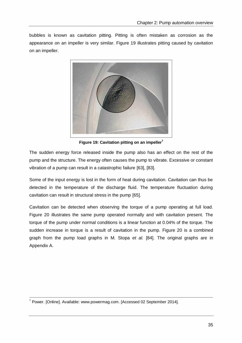
Chapter 2: Pump automation overview
35
bubbles is known as cavitation pitting. Pitting is often mistaken as corrosion as the
appearance on an impeller is very similar. Figure 19 illustrates pitting caused by cavitation
on an impeller.
Figure 19: Cavitation pitting on an impeller7
The sudden energy force released inside the pump also has an effect on the rest of the
pump and the structure. The energy often causes the pump to vibrate. Excessive or constant
vibration of a pump can result in a catastrophic failure [63], [83].
Some of the input energy is lost in the form of heat during cavitation. Cavitation can thus be
detected in the temperature of the discharge fluid. The temperature fluctuation during
cavitation can result in structural stress in the pump [65].
Cavitation can be detected when observing the torque of a pump operating at full load.
Figure 20 illustrates the same pump operated normally and with cavitation present. The
torque of the pump under normal conditions is a linear function at 0.04% of the torque. The
sudden increase in torque is a result of cavitation in the pump. Figure 20 is a combined
graph from the pump load graphs in M. Stopa et al. [84]. The original graphs are in
Appendix A.
7 Power. [Online]. Available: www.powermag.com. [Accessed 02 September 2014].

Chapter 2: Pump automation overview
36
Figure 20: Pump load torque frequency spectrum
The hydrodynamic performance of a pump is immediately affected when cavitation is
present in a pump [51]. In Figure 21 simplified graphs are shown from the pump cavitation
graphs of D. Wu [85]. The head delivered, flow and rotational speed were measured for the
same pump at low and high rotational speed during normal operation and with cavitation
present. The suction pressure of the pump is adjusted to a low pressure with a vacuum
pump creating cavitation. The original graphs can be found in Appendix A.
Figure 21: Various hydrodynamic performances of a pump with and without cavitation
0
0.05
0.1
0.15
0.2
0.25
0.3
0.35
0.4
0.45
0.5
0.55
0.6
370 380 390 400 410 420 430 440 450Pu
mp
to
rqu
e a
bo
ve n
orm
al
torq
ue [
%]
Frequency [Hz]
Normal operating Cavitation present
0
200
400
600
800
1000
1200
0
5
10
15
20
25
30
0
4
8
12
16
20
0 0.5 1 1.5 2
Head
[m
]
Time [s]
Head Rotational speed Flow
Flo
w x
10
-2 [m
/s]
Ro
tati
on
al
sp
eed
[r/
min
]
Low rotational speed without cavitation
0
200
400
600
800
1000
1200
0
5
10
15
20
25
30
0
4
8
12
16
20
0 0.5 1 1.5 2
Head
[m
]
Time [s]
Head Rotational speed Flow
Flo
w x
10
-2 [m
/s]
Ro
tati
on
al
sp
eed
[r/
min
]
Low rotational speed with cavitation
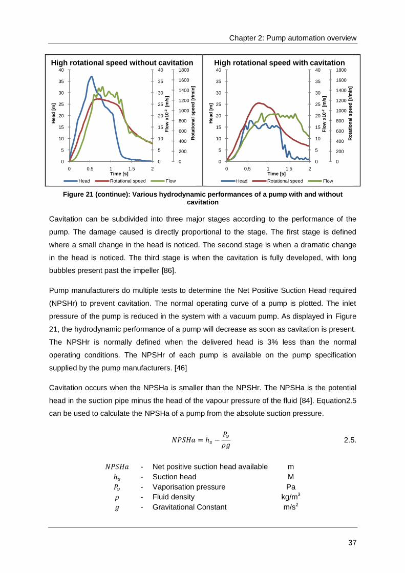
Chapter 2: Pump automation overview
37
Figure 21 (continue): Various hydrodynamic performances of a pump with and without cavitation
Cavitation can be subdivided into three major stages according to the performance of the
pump. The damage caused is directly proportional to the stage. The first stage is defined
where a small change in the head is noticed. The second stage is when a dramatic change
in the head is noticed. The third stage is when the cavitation is fully developed, with long
bubbles present past the impeller [86].
Pump manufacturers do multiple tests to determine the Net Positive Suction Head required
(NPSHr) to prevent cavitation. The normal operating curve of a pump is plotted. The inlet
pressure of the pump is reduced in the system with a vacuum pump. As displayed in Figure
21, the hydrodynamic performance of a pump will decrease as soon as cavitation is present.
The NPSHr is normally defined when the delivered head is 3% less than the normal
operating conditions. The NPSHr of each pump is available on the pump specification
supplied by the pump manufacturers. [46]
Cavitation occurs when the NPSHa is smaller than the NPSHr. The NPSHa is the potential
head in the suction pipe minus the head of the vapour pressure of the fluid [84]. Equation2.5
can be used to calculate the NPSHa of a pump from the absolute suction pressure.
2.5.
- Net positive suction head available m
- Suction head M
- Vaporisation pressure Pa
- Fluid density kg/m3
- Gravitational Constant m/s2
0
200
400
600
800
1000
1200
1400
1600
1800
0
5
10
15
20
25
30
35
40
0
5
10
15
20
25
30
35
40
0 0.5 1 1.5 2
Head
[m
]
Time [s]
Head Rotational speed Flow
Flo
w x
10
-2 [m
/s]
Ro
tati
on
al
sp
eed
[r/
min
]
High rotational speed without cavitation
0
200
400
600
800
1000
1200
1400
1600
1800
0
5
10
15
20
25
30
35
40
0
5
10
15
20
25
30
35
40
0 0.5 1 1.5 2
Head
[m
]
Time [s]
Head Rotational speed Flow
Flo
w x
10
-2 [m
/s]
Ro
tati
on
al
sp
eed
[r/
min
]
High rotational speed with cavitation
Chapter 2: Pump automation overview
38
The potential suction head for the pump system in Figure 8 can be calculated from
Equation 2.6 [84].
2.6.
- Suction head m
- Absolute suction pressure Pa
- Static head of suction pipe m
- Suction nozzle friction head m
- Pipe elbow friction head m
- Suction pipe friction head m
Observing Equation 2.4 where only the pump inlet and outlets are required to calculate the
head of a pump. The NPSHa can thus be calculated through substituting the pump inlet
conditions into Equation 2.5. Equation 2.7 illustrates how the NPSHa can be calculated from
the inlet conditions [51].
2.7.
- Net positive suction head available m
- Inlet pressure Pa
- Inlet velocity m/s
- Vaporisation pressure m
- Fluid density kg/m3
- Gravitational Constant m/s2
To ensure cavitation does not occur, the NPSHa is often designed at NPSHr plus 0.6 m.
This safety factor will limit the cavitation occurrence if the pump is operated outside the
designed conditions. The suction flow is often restricted due to debris in the suction pipeline.
This can result in a suction pressure dropping below the NPSHr [84].

Chapter 2: Pump automation overview
39
2.6. Summary
The characteristics of a multistage centrifugal pump make it one of the most suitable pumps
for dewatering a deep level mine shaft. Multistage centrifugal pumps have the capabilities to
generate the pressure to overcome these high heads. Their proven reliability and robustness
in severe conditions compensate for their cost in this application.
It is clear that neither condition, nor performance monitoring can be neglected when
automating a pump. Condition monitoring is the key aspect protecting the pump against
failure. Performance monitoring compliments condition monitoring to make a more informed
decision on the condition of the pump. Both should be included in the pump automation
program. This will not only ensure safe operation, but improve the reliability of the pump
system.
The correct discharge valve for each pump should be specified in the design. Each valve
type has an advantage for certain applications. The automation of the valve should be kept
in mind when selecting the valve type for automation.
The damage caused by cavitation cannot be neglected. Internal damage has a direct impact
on the life expectancy and efficiency of a pump. Short periods of cavitation also have a direct
impact on the pump performance. Constant cavitation can result in a catastrophic failure and
downtime.
The best practices for pump automation monitor the pump parameters to enable safe
operation. Each instrument installed on the pump system monitors a specific parameter.
These parameters were discussed and found necessary to monitor.
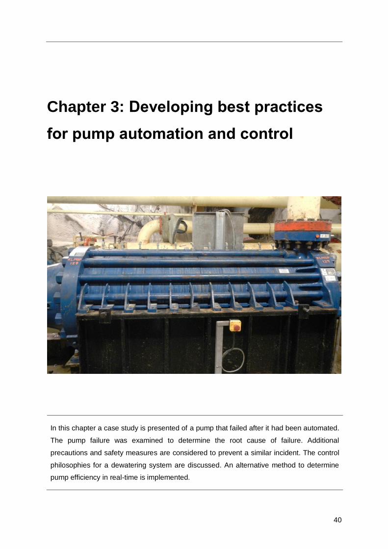
40
Chapter 3: Developing best practices
for pump automation and control
In this chapter a case study is presented of a pump that failed after it had been automated.
The pump failure was examined to determine the root cause of failure. Additional
precautions and safety measures are considered to prevent a similar incident. The control
philosophies for a dewatering system are discussed. An alternative method to determine
pump efficiency in real-time is implemented.

Chapter 3: Developing best practices for pump automation and control
41
3.1. Introduction
A pump automation project was implemented on a deep level mine in the West Rand, South
Africa. The scope of work was to automate the dewatering system of the mine to enable load
shift. Each automated pump was controlled with a dedicated Programmable Logic Controller
(PLC). The PLCs were connected to a Supervisory Control And Data Acquisition system
(SCADA) on surface for a graphical user interface. A real-time energy management system
was used to control the pumps according to the dam levels.
The dewatering system of the mine consists of four pump chambers. The used hot water is
collected at shaft bottom in a settler. The settler separates mining debris and the clear hot
water into different reservoirs. Each pumping chamber has multistage centrifugal pumps and
hot water dams. The pumping chambers are used in an upward cascading manner to
dewater the shaft. Figure 22 shows the layout of the dewatering system of the mine.
3.2. Pump failure analysis
A multistage centrifugal pump on Intermediate Pumping Chamber Main shaft (IPCM) ceased
during the implementation of the project. The pump was operated from the automated
system underground after the automation had been commissioned. Several pump
monitoring instruments and equipment were interlocked in the PLC program.
Unexpected failures of pumps are a major concern. It can result in damage to equipment,
injury and even flooding. Flooding is a high environmental risk for the mining personnel. An
additional concern is the maintenance cost of multistage centrifugal pumps. Refurbishment
cost of a ceased multistage centrifugal pump can reach R 1-million.
Investigations were done to determine the root cause of failure, through examining the
events leading to pump failure. If the causes of failure are known, additional safety systems
can be investigated to prevent similar incidents.
3.2.1. Installed instrumentation and limits
Several condition monitor instruments were originally installed. Each instrument monitors a
specific condition during start-up, running, shut-down or ready-to-start status of the pump.
The installed instrumentation is discussed in the following sections.

Chapter 3: Developing best practices for pump automation and control
42
Figure 22: Dewatering system of the case study mine
SURFACE OPERATIONS AND COOLING
PUMP 2 PUMP 3PUMP 1 PUMP 4
IPC MAIN
LEVEL-22
IPC SUB
PUMP 2 PUMP 3PUMP 1 PUMP 4
LEVEL-46
PUMP 2 PUMP 3PUMP 1
SURFACE
PUMP 4
PUMP 2 PUMP 3PUMP 1 PUMP 4
MIN
ING
OP
ERA
TIO
NS
SLURRY REMOVAL SYSTEM
HOT WATER
DAM
MULTISTAGE
CENTRIFUGAL
PUMP
ELECTRICAL
PUMP MOTOR
ACTUATED
CONTROL
VALVE
NON RETURN
VALVE
3-CPFS
PRESSURE
CHAMBERS
HOT WATER
PIPE
CHILL WATER
PIPE
SLURRY WATER
PIPE
SETTLER
3-CPFS HOT
WATER PIPE
FLOW METER

Chapter 3: Developing best practices for pump automation and control
43
Flow
A digital flow switch was installed on the suction column of the pump. The minimum flow was
set manually on the flow switch. The flow switch ensured that the pump operated within the
minimum flow parameters. The PLC was programmed to disable the flow switch for
two seconds after the motor breaker had closed. This allowed the pump to generate enough
flow during start-up without initiating a trip condition.
The pump motor uses chilled water from the refrigeration plant as cooling medium. A digital
flow switch was installed on the inlet of the pump cooling water pipe. This ensured that the
pump was cooled when the pump was operational.
Each pumping system consists of two discharge columns. Two pumps are connected in
parallel feeding a column per pump station. An analog flow meter is installed on each
discharge column of a pump station. The exact flow each pump delivers can only be
determined if only one pump is operated per column.
A multistage centrifugal pump has a balancing chamber at the discharge side of the pump.
Water enters the chamber between the shaft and the balance disc sleeve. This water acts as
a thin film thrust bearing between the diffusor of the last stage and a balance disc in the
balancing chamber. The pressure in the balancing chamber must not exceed half of the
discharge pressure. To prevent a pressure build-up, a balance disc flow pipe connects the
balancing chamber to the pump inlet.
An analog flow sensor was installed on the balance disc flow pipe of the pump. If the
balance disc sleeve is worn out, the flow through the balance disc flow pipe will increase.
This is also an indication of the wear on the internal components of the pump.
Pressure
These pumps had an efficiency monitoring system installed, which consisted of analog
pressure sensors on the inlet and outlet of the pump. These pressure sensors were
connected to the PLC. The pressure sensors used for performance monitoring, using the
PLC to log the pressure values.
Power
A power meter was installed on the incomer panel of the pump. The power meter measures
the power that each pump consumes. An accurate power measurement is required to
determine the electricity cost saved during the load shift.

Chapter 3: Developing best practices for pump automation and control
44
Vibration
Analog vibration sensors were installed on the motor and pump Drive-End (DE) bearings.
The bearing housings were machine drilled and tapped to install the vibration sensors. Both
vibration sensors were installed in the radial direction with respect to the shaft.
Temperature
Analog temperature probes were installed on the DE and the Non-Drive End (NDE) of both
the motor and the pump. This will detect friction that is induced which will result in a
temperature rise. The friction of the bearings can be a result of failing, incorrectly installed or
incorrect operation of the pump.
The chilled water of the motor acts as a cooling medium for the air of the motor. The cooled
air flows over the windings of the motor. The pump motor has internal winding temperature
probes installed. The winding temperatures of all three phases were included in the PLC
program.
Position switches and sensors
Position switches were installed on the suction butterfly valve of the pump. The switches
were installed to detect if the valve is in the fully open or fully closed position. The PLC will
prevent the pump from running if the valve is not in the fully open position. A trip condition
will be initiated if the valve is closed when the pump is running. This will ensure the suction
valve does not restrict the flow of the pump.
A proximity sensor was installed to detect the pump impeller displacement. The sensor was
set mechanically according the float of the pump. The impeller of a pump moves due to
thrust towards the suction intake when a pump is started. Impeller suction causes the thrust.
The pump will thrust until the pressure in the balancing chamber is enough for the water to
act as a thin film thrust bearing.
The motor has an internal position switch to detect if the cooling water of the motor leaks. A
plate was installed underneath the cooling water pipe inside the air cooling system of the
pump. The weight of the water from a leaking cooling water pipe will displace the plate and
close the connection of the position switch.
An analog motor rotor displacement sensor was installed on the NDE of the motor. The
thrust of the pump during start-up acts on the motor rotor. Once the pump is running at full
load, the rotor must operate in the magnetic centre of the motor. This is the optimal position
for the motor to operate. The rotor displacement sensor ensures that the motor is operated
in its optimal position.
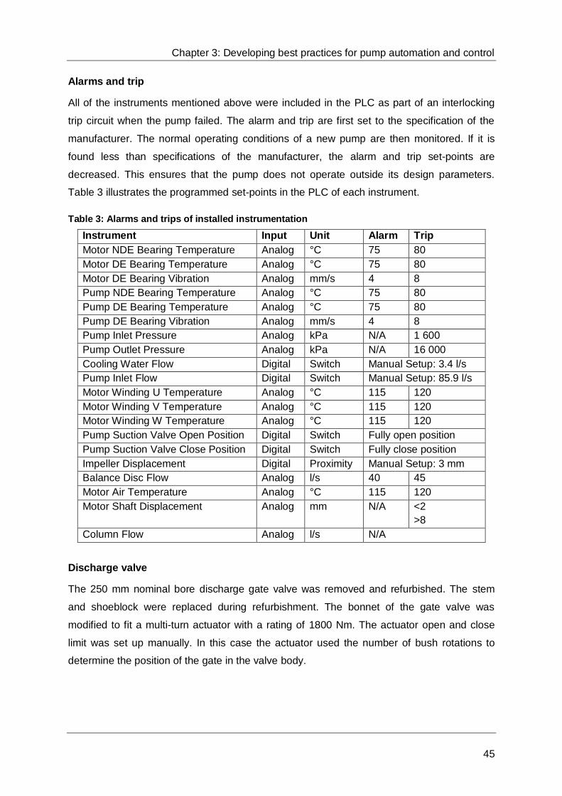
Chapter 3: Developing best practices for pump automation and control
45
Alarms and trip
All of the instruments mentioned above were included in the PLC as part of an interlocking
trip circuit when the pump failed. The alarm and trip are first set to the specification of the
manufacturer. The normal operating conditions of a new pump are then monitored. If it is
found less than specifications of the manufacturer, the alarm and trip set-points are
decreased. This ensures that the pump does not operate outside its design parameters.
Table 3 illustrates the programmed set-points in the PLC of each instrument.
Table 3: Alarms and trips of installed instrumentation
Instrument Input Unit Alarm Trip
Motor NDE Bearing Temperature Analog °C 75 80
Motor DE Bearing Temperature Analog °C 75 80
Motor DE Bearing Vibration Analog mm/s 4 8
Pump NDE Bearing Temperature Analog °C 75 80
Pump DE Bearing Temperature Analog °C 75 80
Pump DE Bearing Vibration Analog mm/s 4 8
Pump Inlet Pressure Analog kPa N/A 1 600
Pump Outlet Pressure Analog kPa N/A 16 000
Cooling Water Flow Digital Switch Manual Setup: 3.4 l/s
Pump Inlet Flow Digital Switch Manual Setup: 85.9 l/s
Motor Winding U Temperature Analog °C 115 120
Motor Winding V Temperature Analog °C 115 120
Motor Winding W Temperature Analog °C 115 120
Pump Suction Valve Open Position Digital Switch Fully open position
Pump Suction Valve Close Position Digital Switch Fully close position
Impeller Displacement Digital Proximity Manual Setup: 3 mm
Balance Disc Flow Analog l/s 40 45
Motor Air Temperature Analog °C 115 120
Motor Shaft Displacement Analog mm N/A <2
>8
Column Flow Analog l/s N/A
Discharge valve
The 250 mm nominal bore discharge gate valve was removed and refurbished. The stem
and shoeblock were replaced during refurbishment. The bonnet of the gate valve was
modified to fit a multi-turn actuator with a rating of 1800 Nm. The actuator open and close
limit was set up manually. In this case the actuator used the number of bush rotations to
determine the position of the gate in the valve body.
Chapter 3: Developing best practices for pump automation and control
46
Human intervention
Although the pump is fully automated, human intervention is still needed. A typical daily task
performed by mine personnel is filling the bearing oil cavity. Condition monitoring decreases
the maintenance frequency but does not completely remove maintenance. The following
safety equipment was installed to reduce human intervention incidents:
Emergency stop at pump,
Emergency stop on PLC panel,
Pump lockout switch on PLC panel,
Start-up warning siren,
Red light to indicate running status,
Blue light to indicate ready to start status,
Green light to indicate a stop status, and
Yellow light to indicate an alarm or trip.
The actuator, instrumentation, safety equipment and power meter were all interlocked in the
PLC program. If any of the conditions monitored does not satisfy a safe pump operating
condition, the pump will trip. An alarm with the trip condition description will be displayed on
the HMI of the PLC. If the condition which initiated the trip is satisfied for safe pump
operation, the PLC can be reset. If the unsafe condition persists, the PLC will prevent the
pump from starting.
3.2.2. Events leading to pump failure
The connection between the shoeblock and stem failed, causing a separation during the
opening of the discharge valve. The gate remained in the closed position. The actuator bush
could still rotate freely, moving the stem to the open position. The actuator determined the
position of the gate by the number of rotations of the bushes inside the actuator. An open
position signal was received by the PLC.
Figure 23 displays a basic diagram of a gate valve. The shoeblock is the connection
between the stem and the disc. The stem of the gate valve was only connected to the
shoeblock with an approximately 10 mm circumferential weld on the top and bottom.

Chapter 3: Developing best practices for pump automation and control
47
NR. DESCRIPTION NR. DESCRIPTION
1 HANDWHEEL 9 SHOEBLOCK
2 GLAND 10 BONNET FASTENERS
3 PACKING 11 BONNET
4 STEM 12 YOKE FASTENERS
5 GASKET 13 YOKE
6 BODY 14 GREASE NIPPLE
7 SEAT RING 15 YOKE SLEEVE
8 DISC
Figure 23: Gate valve diagram
Figure 24 illustrates the failed connection between the stem and shoeblock. Photo a in
Figure 24 displays the bottom of the stem; photo b in Figure 24 displays the top of the
shoeblock; photo c in Figure 24 displays the assembling of the component; and photo d in
Figure 24 displays the gate. The connected stem and shoeblock slide into the key of the
gate on the left to complete the assembly.
1
2
4
3
5
6
7
15
14
13
10
12
11
9
8

Chapter 3: Developing best practices for pump automation and control
48
a)
b)
c)
d)
Figure 24: Gate valve a) spindle; b) shoeblock; c) spindle and shoeblock; and d) gate
A signal to close the motor circuit breaker was sent by the PLC. The motor started rotating
the pump to initiate flow through the pump. The suction flow switch was disabled for
approximately two seconds during the start-up sequence. This allowed the pump to generate
flow before it tripped due to low or no suction flow.
The closed discharge valve resulted in no flow through the pump. Water is seen as an
incompressible fluid. This resulted in the water volume inside the pump staying constant.
The pump generated a pressure, as the design intended to deliver the head. The volume of
the pump and columns are constant due their material properties. This resulted in a
temperature rise from the mentioned constrains and Equation 3.1.
3.1.
- Pressure Pa
- Volume m3
- Amount of substance Mol
- Universal gas constant J/mol.K
- Temperature K
The temperature rise resulted in expansion of the internal parts of the pump. The clearance
between the internal parts is designed to a minimum to decrease internal pump pressure
loss. The expansion led to friction between the rotating pump impellers and the stationary
pump casing and diffusors. This resulted in a drastic secondary increase of the temperature.

Chapter 3: Developing best practices for pump automation and control
49
3.2.3. Possible cause of valve failure
It is evident that the root cause of failure was the discharge valve that failed to open. The
failure of the discharge valve resulted in a chain of events which resulted in pump failure. An
investigation of the forces and pressures acting on the gate of the valve was launched to
determine the possible reason of failure.
If the gate exceeds the close position, the gate is forced into the seat. If the gate was forced
into the seat more force was required to open the valve. When the valve was opened for
investigation, the gate was loose and could be moved freely by hand. This is an indication
that the close limit of the actuator was set correctly and the gate was not forced into the seat.
Similar to the close limit, the actuator can cause damage to the valve if the open limit is set
incorrectly. When the open position is exceeded, the shoeblock and gate is forced into the
bonnet of the valve. The shoeblock is normally bent when the open limit is exceeded. Since
the shoeblock was not bent, the open limit had been set-up correctly. Both the possibilities of
the open and close limits set incorrectly were thus eliminated.
The torque limits of the actuator could have been set incorrectly. This would have resulted in
the actuator applying more force than the valve was designed and manufactured to handle.
If the sum of all forces applied to a body has an equilibrium force in one direction, the body
will accelerate. This is shown with Equation 3.2.
3.2.
- Equivalent force N
- Mass kg
- Acceleration m/s2
The equilibrium force acting on the gate was zero, because the valve failed in a closed
position. Another force must have been present to counteract the actuator force applied. The
static friction force is the only force acting against the direction of the actuator force. This
resulted in the zero equilibrium force of the gate. The static friction force is defined with
Equation 3.3.
3.3.
- Static friction force N
- Normal force N
- Friction coefficient -

Chapter 3: Developing best practices for pump automation and control
50
The normal force, acting on the gate of the valve is generated by the head of the water
above the valve. The water creates pressure which acts on the gate of the valve. The
pressure of the fluid at the discharge valve is defined with Equation 3.4.
3.4.
- Pressure of head Pa
- Fluid density kg/m3
- Head m
- Gravitational Constant m/s2
A Non-Return Valve (NRV) is installed between the pump and the discharge valve. Figure 25
displays the arrangement in with the valves are installed. The pump is stopped when the
discharge valve is 5% open. This ensures the NRV seals properly and prevents the
discharge valve from exceeding the maximum torque limit while closing. Some of the
pressure is stored as potential pressure between the NRV and the gate valve.
Figure 25: Discharge valve and NRV installed arrangement
If the NRV does not seal properly, the water leaks through to the pump. The potential
pressure stored between the discharge valve and the NRV when the pump is stopped, will
be lost. This results in a differential pressure across the valve. The differential pressure
creates the normal force acting on the gate of the valve. The differential pressure across the
valve is defined in Equation 3.5.
DISCHARGE VALVE
NRV

Chapter 3: Developing best practices for pump automation and control
51
3.5.
- Differential pressure across valve Pa
- Pressure of head Pa
- Stored potential pressure Pa
The forces as a result of pressure inside a closed body, act perpendicular on the inner walls
of the body. The diameter of the discharge valve gate is known. The force acting on the gate
as a result of the pressure is defined with Equation 3.6. This force is also equal to the normal
force acting on the gate of the valve.
3.6.
- Normal force N
- Differential pressure across valve Pa
- Area of the valve Pa
Substituting Equation 3.4, 3.5 and 3.6 into Equation 3.3 gives the resultant force due to the
pressure difference across the valve. Equation 3.7 illustrates the substituted equation. It is
clear from the equation that the smaller potential energy is stored between the NRV and
gate valve, the greater the friction force will be. The other variables can be seen as constant
with the head at a maximum when the discharge column is full.
3.7.
- Static friction force N
- Fluid density kg/m3
- Head m
- Gravitational Constant m/s2
- Stored potential pressure Pa
- Area of the valve Pa
This shows that if the torque limit of the actuator was set incorrectly, another force must
have been present preventing the gate from moving. The secondary force was a result of a
leaking NRV creating a differential pressure across the valve. There were no other forces
found to act as the reaction force.
3.2.4. Pump disassembled examination
Figure 26 displays a diagram of a six stage centrifugal pump. The components of the pump
are numbered and displayed in the table of the figure. The figure shows where the

Chapter 3: Developing best practices for pump automation and control
52
components of the pump are located. A 12-stage centrifugal pump has similar components,
only with double the number of stages.
19202122 17 15 1416 13 12 11 10
2 63 5 71
1823 89
4
NR. DESCRIPTION NR. DESCRIPTION
1 STUFFING BOX HOUSING 13 STAGE CASING
2 INLET CASING 14 WEAR RING
3 INLET 15 WEAR RING
4 ASSEMBLY FASTENER 16 IMPELLER
5 OUTLET 17 DIFFUSOR
6 OUTLET CASING 18 SHAFT
7 BALANCE DISC CHAMBER 19 PACKING
8 IMPELLER DISPLACEMENT 20 PACKING GLAND
9 PUMP NDE 21 O-RING
10 SHAFT SLEEVE 22 BEARING
11 BALANCE DISC 23 PUMP DE
12 BALANCE RING
Figure 26: Six stage centrifugal pump diagram
The seized pump was sent for repairs. Access was arranged to do a visual examination of
the pump when it was disassembled. The pump had only been installed and operated for
two months before it seized. It was assumed that any visible sign of damage found on the
pump was caused by the recent failure.
The casing neck ring is a stationary component installed on the pump casing. It acts as
protection between the pump casing and the shroud of the rotating impeller. The clearance
between the impeller neck and the casing neck ring for normal operation is 0.2 mm on each
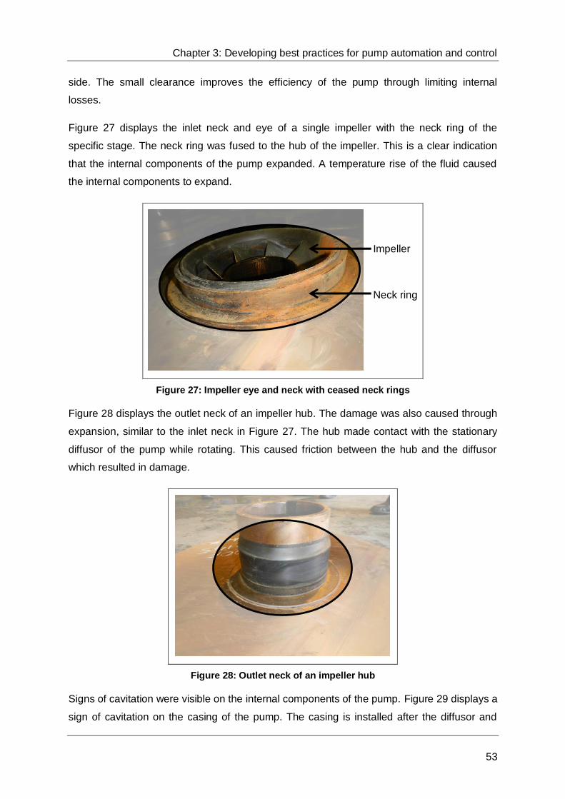
Chapter 3: Developing best practices for pump automation and control
53
side. The small clearance improves the efficiency of the pump through limiting internal
losses.
Figure 27 displays the inlet neck and eye of a single impeller with the neck ring of the
specific stage. The neck ring was fused to the hub of the impeller. This is a clear indication
that the internal components of the pump expanded. A temperature rise of the fluid caused
the internal components to expand.
Figure 27: Impeller eye and neck with ceased neck rings
Figure 28 displays the outlet neck of an impeller hub. The damage was also caused through
expansion, similar to the inlet neck in Figure 27. The hub made contact with the stationary
diffusor of the pump while rotating. This caused friction between the hub and the diffusor
which resulted in damage.
Figure 28: Outlet neck of an impeller hub
Signs of cavitation were visible on the internal components of the pump. Figure 29 displays a
sign of cavitation on the casing of the pump. The casing is installed after the diffusor and
Impeller
Neck ring

Chapter 3: Developing best practices for pump automation and control
54
before the inlet of the next impeller. The erosion in the casing was caused by the imploding
bubbles.
Figure 29: Sign of cavitation on casing
Cavitation occurs when the static pressure drops below vapour pressure. The inlet of the
pump was not restricted, thus the pressure could not have been below vapour pressure. The
reason for cavitation was that the temperature exceeded the vapour temperature at the
specific pressure. This resulted in vapour forming in the water.
The failed discharge valve induced a pressure increase on the outlet side of the pump. This
pressure resulted in an additional force being applied on the outlet of each impeller. The
force caused the balance disc to make contact with the outlet casing. Figure 30 displays the
wear found on the outlet casing.
Figure 30: Friction on the outlet casing due to balance disc
The balance disc wear is manufactured with a bronze wear ring and a steel wear ring. The
minimum thickness of a balance disc wear ring is 37 mm. This prevents the impeller shrouds
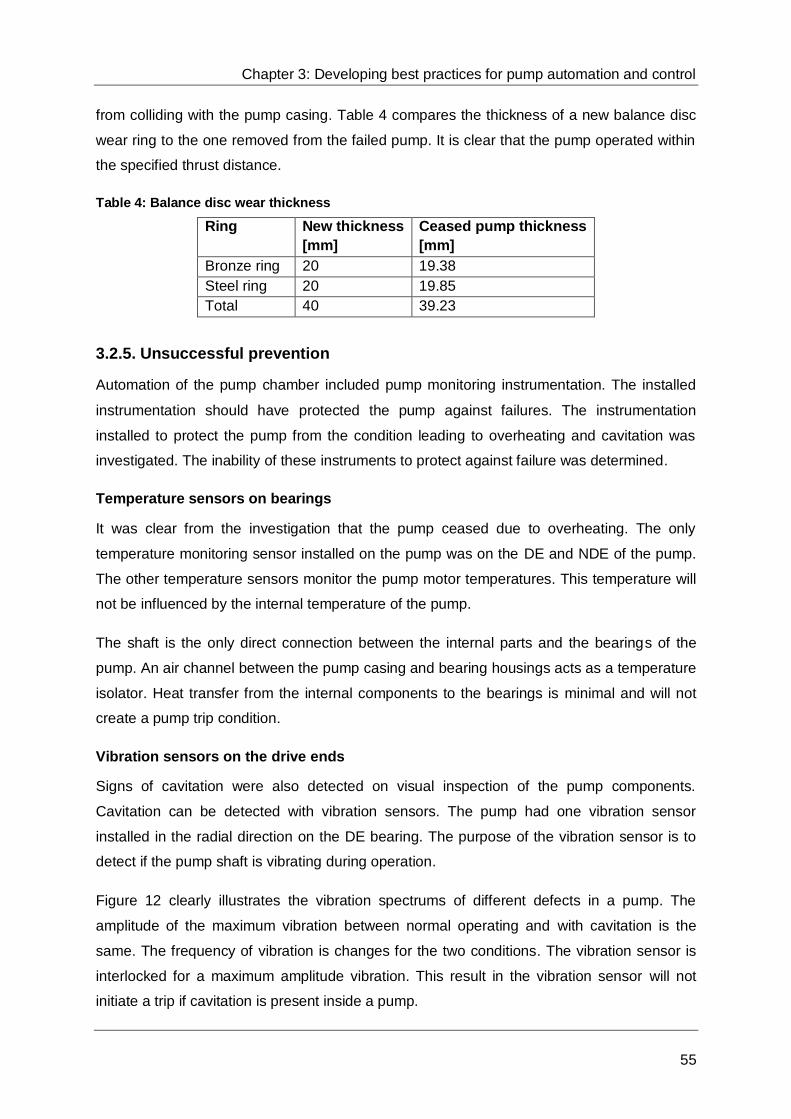
Chapter 3: Developing best practices for pump automation and control
55
from colliding with the pump casing. Table 4 compares the thickness of a new balance disc
wear ring to the one removed from the failed pump. It is clear that the pump operated within
the specified thrust distance.
Table 4: Balance disc wear thickness
Ring New thickness
[mm]
Ceased pump thickness
[mm]
Bronze ring 20 19.38
Steel ring 20 19.85
Total 40 39.23
3.2.5. Unsuccessful prevention
Automation of the pump chamber included pump monitoring instrumentation. The installed
instrumentation should have protected the pump against failures. The instrumentation
installed to protect the pump from the condition leading to overheating and cavitation was
investigated. The inability of these instruments to protect against failure was determined.
Temperature sensors on bearings
It was clear from the investigation that the pump ceased due to overheating. The only
temperature monitoring sensor installed on the pump was on the DE and NDE of the pump.
The other temperature sensors monitor the pump motor temperatures. This temperature will
not be influenced by the internal temperature of the pump.
The shaft is the only direct connection between the internal parts and the bearings of the
pump. An air channel between the pump casing and bearing housings acts as a temperature
isolator. Heat transfer from the internal components to the bearings is minimal and will not
create a pump trip condition.
Vibration sensors on the drive ends
Signs of cavitation were also detected on visual inspection of the pump components.
Cavitation can be detected with vibration sensors. The pump had one vibration sensor
installed in the radial direction on the DE bearing. The purpose of the vibration sensor is to
detect if the pump shaft is vibrating during operation.
Figure 12 clearly illustrates the vibration spectrums of different defects in a pump. The
amplitude of the maximum vibration between normal operating and with cavitation is the
same. The frequency of vibration is changes for the two conditions. The vibration sensor is
interlocked for a maximum amplitude vibration. This result in the vibration sensor will not
initiate a trip if cavitation is present inside a pump.

Chapter 3: Developing best practices for pump automation and control
56
Position of the discharge valve gate
The actuator of the discharge valve uses the number of rotations to determine the position of
the gate. The actuator raises the stem through rotating the bush inside the actuator. This
acts as a screw jack gear system and raises the gate inside the valve. The body of the valve
guides the gate to prevent it from rotating.
The broken connection between the gate and the spindle made that the spindle could still
move freely. The actuator received an open position signal because the actuator completed
the number of turns. This prevented the PLC to initiate the trip sequence for a close
discharge valve.
Flow switch on suction column
Zero to low flow through the pump was caused by the discharge valve that failed to open
caused. The flow switch is activated in the PLC program two seconds after the motor
breaker closes. It should have initiated the trip sequence. The minimum required flow set
manually on the flow switch was met. This caused the pump to continue to run with low flow.
When the efficiency of a pump starts to deteriorates, the minimum flow is not delivered. Mine
personnel often reduce manual set limit on the flow switch when it is insufficient. This
prevents the PLC to initiate the trip sequence and allow for pumping. The reduced limit on
the flow switch did not detect the low flow through the pump when the valve failed.
Discharge pressure
The main purpose of the installed discharge pressure was to monitor the performance of the
pump. A trip set-point for the pressure was programmed into the PLC. The maximum rated
pump discharge pressure is 12.3 MPa at a low flow. The trip set-point of the pressure was
set at 16.0 MPa. The pump was not capable to generate enough pressure to reach the trip
set-point.
3.3. Improved design to prevent failure
The pump failure is proof that the automation and safety circuit of the pump did not cater for
all failure conditions. The current practice in which the client specifies automation has to be
improved to prevent similar incidents. Immediate precautions had to be taken because the
automation project was already commissioned. Several solutions were investigated to
prevent similar incidents.

Chapter 3: Developing best practices for pump automation and control
57
3.3.1. Differential pressure over discharge valve
The evident proof of the presence of a differential pressure across the discharge valve led to
the first solution. It was proposed that a pressure sensor be installed between the NRV and
the discharge valve and another sensor after the discharge valve. This could be used to
determine the differential pressure across the valve.
The NRV and the discharge valve flanges are directly next to each other. Installing a
pressure sensor between the valves was impossible. Installing the pressure sensor between
the pump and the NRV will not measure the differential pressure across the discharge valve.
The NRV will act as pressure isolation.
Further investigation of the discharge valve application showed that pressure equalising
valves were available. Figure 31 illustrates a gate valve with a manual bypass valve. By
opening the bypass valve before opening the main valve, the pressure across the valve will
be equalised. These types of valve are designed for high pressure application, which often
has a differential pressure.
Figure 31: High pressure gate valve with pressure equalizing bypass8
The pressure differential will only be created if the NRV leaks. If the NRV leaks and the
bypass valve remains in the open position, the discharge column will be drained. In this case
the bypass valve has to be in the closed manually. This defies the purpose of automation if
the bypass valve has to be opened manually. The cost of the new valves and automating the
bypass valve is not feasible.
8 Xinhai Valve. [Online]. Available: www.xhvalves.com. [Accessed 02 September 2014].
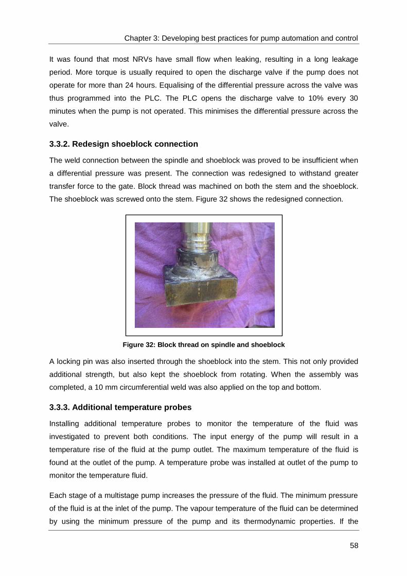
Chapter 3: Developing best practices for pump automation and control
58
It was found that most NRVs have small flow when leaking, resulting in a long leakage
period. More torque is usually required to open the discharge valve if the pump does not
operate for more than 24 hours. Equalising of the differential pressure across the valve was
thus programmed into the PLC. The PLC opens the discharge valve to 10% every 30
minutes when the pump is not operated. This minimises the differential pressure across the
valve.
3.3.2. Redesign shoeblock connection
The weld connection between the spindle and shoeblock was proved to be insufficient when
a differential pressure was present. The connection was redesigned to withstand greater
transfer force to the gate. Block thread was machined on both the stem and the shoeblock.
The shoeblock was screwed onto the stem. Figure 32 shows the redesigned connection.
Figure 32: Block thread on spindle and shoeblock
A locking pin was also inserted through the shoeblock into the stem. This not only provided
additional strength, but also kept the shoeblock from rotating. When the assembly was
completed, a 10 mm circumferential weld was also applied on the top and bottom.
3.3.3. Additional temperature probes
Installing additional temperature probes to monitor the temperature of the fluid was
investigated to prevent both conditions. The input energy of the pump will result in a
temperature rise of the fluid at the pump outlet. The maximum temperature of the fluid is
found at the outlet of the pump. A temperature probe was installed at outlet of the pump to
monitor the temperature fluid.
Each stage of a multistage pump increases the pressure of the fluid. The minimum pressure
of the fluid is at the inlet of the pump. The vapour temperature of the fluid can be determined
by using the minimum pressure of the pump and its thermodynamic properties. If the
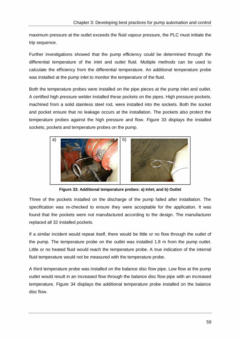
Chapter 3: Developing best practices for pump automation and control
59
maximum pressure at the outlet exceeds the fluid vapour pressure, the PLC must initiate the
trip sequence.
Further investigations showed that the pump efficiency could be determined through the
differential temperature of the inlet and outlet fluid. Multiple methods can be used to
calculate the efficiency from the differential temperature. An additional temperature probe
was installed at the pump inlet to monitor the temperature of the fluid.
Both the temperature probes were installed on the pipe pieces at the pump inlet and outlet.
A certified high pressure welder installed these pockets on the pipes. High pressure pockets,
machined from a solid stainless steel rod, were installed into the sockets. Both the socket
and pocket ensure that no leakage occurs at the installation. The pockets also protect the
temperature probes against the high pressure and flow. Figure 33 displays the installed
sockets, pockets and temperature probes on the pump.
a)
b)
Figure 33: Additional temperature probes: a) Inlet; and b) Outlet
Three of the pockets installed on the discharge of the pump failed after installation. The
specification was re-checked to ensure they were acceptable for the application. It was
found that the pockets were not manufactured according to the design. The manufacturer
replaced all 32 installed pockets.
If a similar incident would repeat itself, there would be little or no flow through the outlet of
the pump. The temperature probe on the outlet was installed 1.8 m from the pump outlet.
Little or no heated fluid would reach the temperature probe. A true indication of the internal
fluid temperature would not be measured with the temperature probe.
A third temperature probe was installed on the balance disc flow pipe. Low flow at the pump
outlet would result in an increased flow through the balance disc flow pipe with an increased
temperature. Figure 34 displays the additional temperature probe installed on the balance
disc flow.
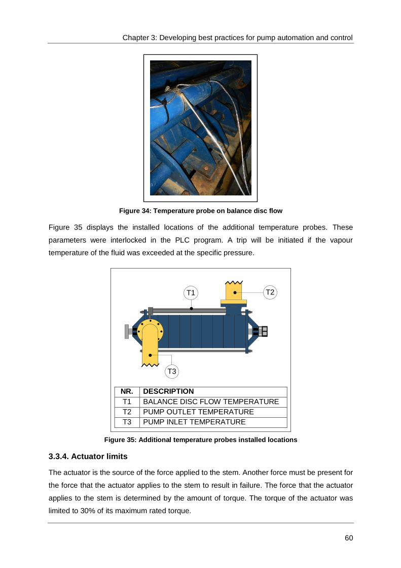
Chapter 3: Developing best practices for pump automation and control
60
Figure 34: Temperature probe on balance disc flow
Figure 35 displays the installed locations of the additional temperature probes. These
parameters were interlocked in the PLC program. A trip will be initiated if the vapour
temperature of the fluid was exceeded at the specific pressure.
NR. DESCRIPTION
T1 BALANCE DISC FLOW TEMPERATURE
T2 PUMP OUTLET TEMPERATURE
T3 PUMP INLET TEMPERATURE
Figure 35: Additional temperature probes installed locations
3.3.4. Actuator limits
The actuator is the source of the force applied to the stem. Another force must be present for
the force that the actuator applies to the stem to result in failure. The force that the actuator
applies to the stem is determined by the amount of torque. The torque of the actuator was
limited to 30% of its maximum rated torque.
T3
T1 T2

Chapter 3: Developing best practices for pump automation and control
61
The open and close limits of the actuator were also verified. Incorrect configured open or
close limits can result in damage to the stem, shoeblock, gate, seats and actuator.
Maximum torque is required for initial opening of the valve. As soon as the pressure across
the valve is equalised, a minimum of 5% of the rated torque is required to move the gate.
The minimum torque is required to overcome the internal friction of the valve and actuator. If
the connection between the spindle and shoeblock fails, the friction will decline, resulting in
reduced torque. An under torque limit of 5% was set on the actuator during gate movement.
3.3.5. Suction flow sensor protection
The suspicion of tampering with the suction flow sensor led to a password protection
investigation. A digital installed flow switch was installed on the suction of the pump. The trip
set-points of digital instruments were set manually on the instrument. A digital instrument
only returns an open or close feedback. This results that the trip set-point cannot be
interlocked in the PLC program.
The installed suction flow switch could only be locked instead of password protected.
Minimum flow was set and locked on the flow switches according to tested flows of each
pump. The locking and unlocking procedure could not be changed. It is of utmost importance
that only authorised personnel receive the procedure.
3.4. Optimised pump control
The automated pump system allowed for remote safely control of the pump system. To
maximise potential savings, a dynamic pump scheduling program was implemented. The
program determines the pump schedule according to the real-time dam levels. The pump
load is reduced with the program to a minimum during the more expensive electricity peak
periods. Several interlocks are programmed into the software to ensure the water is
managed safely.
3.4.1. Input parameters
The more expensive electricity peak periods are from 7:00 to 10:00 and 18:00 to 20:00. The
mine requested to extend the period of minimum pump load. The minimum pump load is
programmed from 6:45 to 10:00 and 16:45 to 20:00. Defining the correct control limits will
create enough capacity to extend the peak periods.
The full storage potential of mine dams is seldom used. The settlers do not remove all the
debris from the water, which settles in the clear water dams. The minimum dam levels of the

Chapter 3: Developing best practices for pump automation and control
62
dams are thus increased. To reduce the risk of flooding the maximum dam levels are also
limited. Table 5 displays the maximum and minimum specified dam limits at this mine.
Table 5: Maximum and minimum dam limits
Pump chamber Minimum dam level [%] Maximum dam level [%]
IPCM 3-CPFS Off 30 95
IPCM 3-CPFS On 60 95
Level-22 30 95
IPCS 50 90
Level-46 20 95
The 3-CPFS and the pumps on IPCM use the same dewatering column. This increases the
risk of failure due to the pressure and decreases the system efficiency. The pumps must be
limited to a maximum two when the 3-CPFS is running.
3.4.2. Control dams
All pump chambers have more than one dam. The total dam storage capacity is determined
through the availability of the dams. The dams of each pump chamber are connected with a
pipe and an isolation valve. During normal operation the isolation valves are open. The
pump schedule is determined with a control dam. The control dam level is calculated from
the average dam levels of the dams available.
Hot water dams are often contaminated with mud. The mud acts as a corrosion agent on the
pumps when it is pumped with water. This results in additional wear on the internal parts of
the pumps. The mud has a direct influence on the minimum dam level and storage capacity.
The isolation valve is closed when the specific dam is drained to clean and remove the mud.
Isolated dam levels are excluded from the control dam average.
3.4.3. Hold commands
The 3-CPFS is not controlled with the dynamic pump scheduling program. The 3-CPFS has
four pump running statuses and a pause status. Different combinations of the statuses result
in different amounts of flow delivered. Table 6 displays the flow the 3-CPFS deliver for
different pump status combinations.
Table 6: 3-CPFS flow from its pump status combinations
Pump 1 Pump 2 Pump 3 Pump 4 Paused Flow [l/s]
1 1 - 1 - 320
- - 1 1 - 140
- - - - 1 0
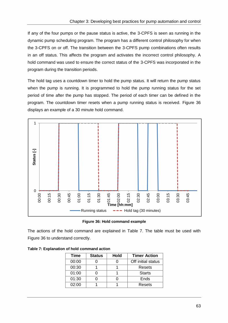
Chapter 3: Developing best practices for pump automation and control
63
If any of the four pumps or the pause status is active, the 3-CPFS is seen as running in the
dynamic pump scheduling program. The program has a different control philosophy for when
the 3-CPFS on or off. The transition between the 3-CPFS pump combinations often results
in an off status. This affects the program and activates the incorrect control philosophy. A
hold command was used to ensure the correct status of the 3-CPFS was incorporated in the
program during the transition periods.
The hold tag uses a countdown timer to hold the pump status. It will return the pump status
when the pump is running. It is programmed to hold the pump running status for the set
period of time after the pump has stopped. The period of each timer can be defined in the
program. The countdown timer resets when a pump running status is received. Figure 36
displays an example of a 30 minute hold command.
Figure 36: Hold command example
The actions of the hold command are explained in Table 7. The table must be used with
Figure 36 to understand correctly.
Table 7: Explanation of hold command action
Time Status Hold Timer Action
00:00 0 0 Off initial status
00:30 1 1 Resets
01:00 0 1 Starts
01:30 0 0 Ends
02:00 1 1 Resets
0
1
00
:00
00
:15
00
:30
00
:45
01
:00
01
:15
01
:30
01
:45
02
:00
02
:15
02
:30
02
:45
03
:00
03
:15
03
:30
03
:45
Sta
tus
[-]
Time [hh:mm]
Running status Hold tag (30 minutes)
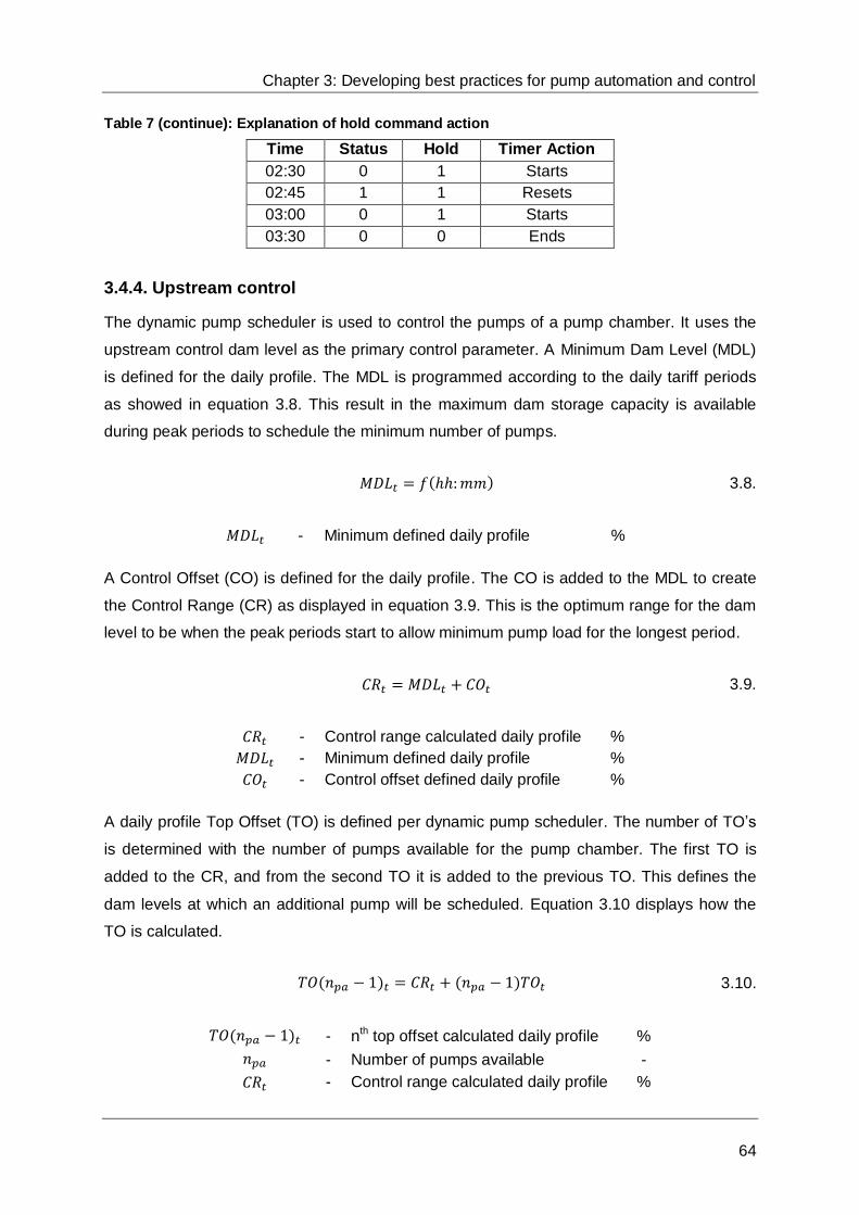
Chapter 3: Developing best practices for pump automation and control
64
Table 7 (continue): Explanation of hold command action
Time Status Hold Timer Action
02:30 0 1 Starts
02:45 1 1 Resets
03:00 0 1 Starts
03:30 0 0 Ends
3.4.4. Upstream control
The dynamic pump scheduler is used to control the pumps of a pump chamber. It uses the
upstream control dam level as the primary control parameter. A Minimum Dam Level (MDL)
is defined for the daily profile. The MDL is programmed according to the daily tariff periods
as showed in equation 3.8. This result in the maximum dam storage capacity is available
during peak periods to schedule the minimum number of pumps.
3.8.
- Minimum defined daily profile %
A Control Offset (CO) is defined for the daily profile. The CO is added to the MDL to create
the Control Range (CR) as displayed in equation 3.9. This is the optimum range for the dam
level to be when the peak periods start to allow minimum pump load for the longest period.
3.9.
- Control range calculated daily profile %
- Minimum defined daily profile %
- Control offset defined daily profile %
A daily profile Top Offset (TO) is defined per dynamic pump scheduler. The number of TO’s
is determined with the number of pumps available for the pump chamber. The first TO is
added to the CR, and from the second TO it is added to the previous TO. This defines the
dam levels at which an additional pump will be scheduled. Equation 3.10 displays how the
TO is calculated.
3.10.
- nth top offset calculated daily profile %
- Number of pumps available -
- Control range calculated daily profile %
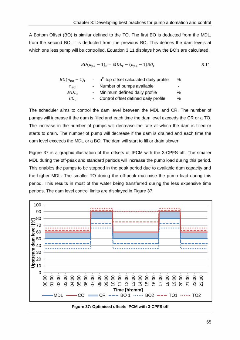
Chapter 3: Developing best practices for pump automation and control
65
A Bottom Offset (BO) is similar defined to the TO. The first BO is deducted from the MDL,
from the second BO, it is deducted from the previous BO. This defines the dam levels at
which one less pump will be controlled. Equation 3.11 displays how the BO’s are calculated.
3.11.
- nth top offset calculated daily profile %
- Number of pumps available -
- Minimum defined daily profile %
- Control offset defined daily profile %
The scheduler aims to control the dam level between the MDL and CR. The number of
pumps will increase if the dam is filled and each time the dam level exceeds the CR or a TO.
The increase in the number of pumps will decrease the rate at which the dam is filled or
starts to drain. The number of pump will decrease if the dam is drained and each time the
dam level exceeds the MDL or a BO. The dam will start to fill or drain slower.
Figure 37 is a graphic illustration of the offsets of IPCM with the 3-CPFS off. The smaller
MDL during the off-peak and standard periods will increase the pump load during this period.
This enables the pumps to be stopped in the peak period due to available dam capacity and
the higher MDL. The smaller TO during the off-peak maximise the pump load during this
period. This results in most of the water being transferred during the less expensive time
periods. The dam level control limits are displayed in Figure 37.
Figure 37: Optimised offsets IPCM with 3-CPFS off
0
10
20
30
40
50
60
70
80
90
100
00:0
0
01:0
0
02:0
0
03:0
0
04:0
0
05:0
0
06:0
0
07:0
0
08:0
0
09:0
0
10:0
0
11:0
0
12:0
0
13:0
0
14:0
0
15:0
0
16:0
0
17:0
0
18:0
0
19:0
0
20:0
0
21:0
0
22:0
0
23:0
0
Up
str
ea
m d
am
le
ve
l [%
]
Time [hh:mm]
MDL CO CR BO 1 BO2 TO1 TO2

Chapter 3: Developing best practices for pump automation and control
66
Table 8 displays the defined varying dam limits during a 24-hour profile. The MDL is
increased with 30% during the more expensive peak periods. This allows for the stopping of
the pumps during this period.
Table 8: Optimised offsets for IPCM with 3-CPFS off
Start
[hh:mm]
End
[hh:mm]
MDL
[%]
BO
[%]
CO
[%]
TO
[%]
00:00 6:44 50 7 10 3
06:45 9:59 80 7 10 5
10:00 16:45 50 7 10 15
16:46 19:59 80 7 10 5
20:00 23:59 50 7 10 3
The 3-CPFS has a higher control privilege. The offsets of the pumps are adjusted when a
hold command running status is received from the 3-CPFS. A higher dam level is maintained
on IPCM to ensure the maximum potential of the 3-CPFS is utilised. Figure 38 displays the
input parameters of IPCM when the 3-CPFS is running. The optimised control schedules for
the other three levels can be found in Appendix C.
Figure 38: Optimised offsets IPCM with 3-CPS on
Table 9 displays the defined input when the 3-CPFS is running. The higher MDL during the
standard and off-peak periods allows for maximum operation of the 3-CPFS.
0
10
20
30
40
50
60
70
80
90
100
00:0
0
01:0
0
02:0
0
03:0
0
04:0
0
05:0
0
06:0
0
07:0
0
08:0
0
09:0
0
10:0
0
11:0
0
12:0
0
13:0
0
14:0
0
15:0
0
16:0
0
17:0
0
18:0
0
19:0
0
20:0
0
21:0
0
22:0
0
23:0
0
Up
str
ea
m d
am
le
ve
l [%
]
Time [hh:mm]
MDL CO CR BO 1 TO1

Chapter 3: Developing best practices for pump automation and control
67
Table 9: Optimised offsets for IPCM with 3-CPS on
Start
[hh:mm]
End
[hh:mm]
MDL
[%]
BO
[%]
CO
[%]
TO
[%]
00:00 6:44 70 5 10 10
06:45 9:59 80 5 10 5
10:00 16:45 70 5 10 10
16:46 19:59 80 5 10 5
20:00 23:59 70 5 10 10
3.4.5. Stable Values
The dam levels of an automation project are usually determined with ultra-sonic level
transmitters or pressure transmitters. Both these sensors determine the dam level relevant
to their installed positions. A small fluctuation is often found with both transmitters. The
fluctuation can interfere with the pump control. Stable values are used to prevent pump
cycling due to this fluctuation.
Stable values can be described as trailing memory tags. The two types of stable values used
are top stable and bottom trailing types. The top stable value remains at the last maximum
value the dam level has reached when the actual value starts to decrease. The top stable
will decrease at the same rate of the dam level, when the difference between the top stable
and actual value is equal to the set limit. When the dam level starts to increase, the top
stable will remain the minimum value reached. The top stable will increase with the actual
dam level when the actual dam level is equal or larger than the minimum value reached.
The stable values used for the control dams are shown in Table 10. This prevents the pumps
from cycling due to dam level fluctuation. Pump cycling increases pump maintenance as
mentioned in Section 1.4.
Table 10: Stable values of control dams
Control dam Stable 1 Stable 2
Surf 10 10
IPCM 15 15
Level-22 5 5
IPCS 5 5
Level-46 5 5
Figure 39 graphically displays a top stable and bottom stable values with the actual dam
level. Both are set to a 10% stable value. The stable values were set equal to the actual at
the start.

Chapter 3: Developing best practices for pump automation and control
68
Figure 39: Stable value example
3.4.6. Number of pumps
The upstream control relies on the water balance being kept in the optimal range with all the
pumps available. As this is only achievable in an ideal world, an additional safety precaution
is required. The downstream dam level is also monitored with the pump scheduler. This will
prevent the downstream dam from flooding as a result of a high inflow.
The downstream dam level limits the maximum number of pumps available to schedule. If
both the upstream and downstream dam levels are almost full, the maximum number of
pumps is set to the number of pumps available. This will pump the excess water to the
surface as a precaution measure. The running status of 3-CPFS also influences the number
of pumps available to schedule on IPCM.
The number of pumps available is adjusted with multiple if-functions, hold commands and
stable values. Table 11 illustrates the different parameters and results for IPCM. The table is
used per column from the first to the last. The applicable situation is selected in each column
as described in the column heading. Only an option from the row of the previous selected
situations can be selected in the subsequent column. The maximum number of pumps
available to schedule is returned in the last column. The maximum number of pumps tables
for the other three levels can be seen in Appendix C.
0
10
20
30
40
50
60
70
80
90
00:0
0
01:0
0
02:0
0
03:0
0
04:0
0
05:0
0
06:0
0
07:0
0
08:0
0
09:0
0
10:0
0
11:0
0
12:0
0
13:0
0
14:0
0
15:0
0
16:0
0
17:0
0
18:0
0
19:0
0
20:0
0
21:0
0
22:0
0
23:0
0
Dam
level
[%]
Time [hh:mm]
Actual dam level Top stable Bottom stable
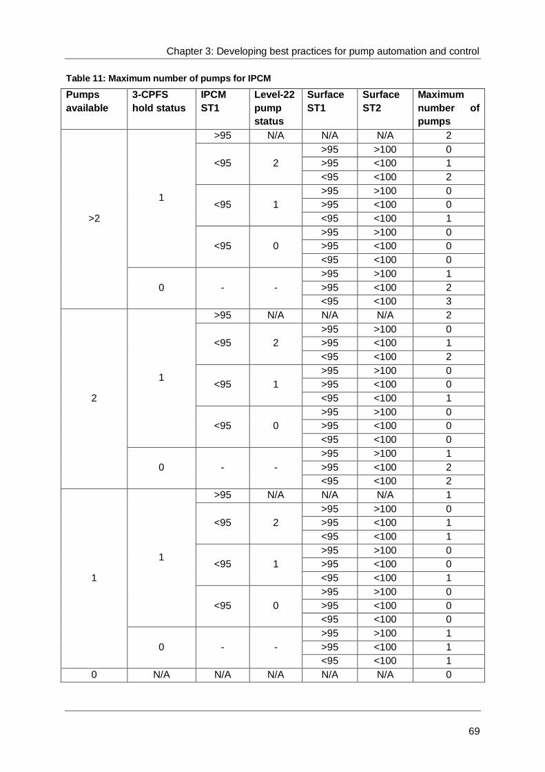
Chapter 3: Developing best practices for pump automation and control
69
Table 11: Maximum number of pumps for IPCM
Pumps
available
3-CPFS
hold status
IPCM
ST1
Level-22
pump
status
Surface
ST1
Surface
ST2
Maximum
number of
pumps
>2
1
>95 N/A N/A N/A 2
<95 2
>95 >100 0
>95 <100 1
<95 <100 2
<95 1
>95 >100 0
>95 <100 0
<95 <100 1
<95 0
>95 >100 0
>95 <100 0
<95 <100 0
0 - -
>95 >100 1
>95 <100 2
<95 <100 3
2
1
>95 N/A N/A N/A 2
<95 2
>95 >100 0
>95 <100 1
<95 <100 2
<95 1
>95 >100 0
>95 <100 0
<95 <100 1
<95 0
>95 >100 0
>95 <100 0
<95 <100 0
0 - -
>95 >100 1
>95 <100 2
<95 <100 2
1
1
>95 N/A N/A N/A 1
<95 2
>95 >100 0
>95 <100 1
<95 <100 1
<95 1
>95 >100 0
>95 <100 0
<95 <100 1
<95 0
>95 >100 0
>95 <100 0
<95 <100 0
0 - -
>95 >100 1
>95 <100 1
<95 <100 1
0 N/A N/A N/A N/A N/A 0

Chapter 3: Developing best practices for pump automation and control
70
3.4.7. Enhancing of control
The control parameters explained in the previous sections are the optimised parameters.
The optimised parameters were achieved through a series of simulation from a basic model.
Small adjustments were made with each simulation until the optimum was achieved.
The offsets for the basic model are achieved with a water balance equation. It is important to
convert the dam level percentage to water volume for the calculation. Equation 3.12
illustrates how to determine the dam levels to enable a maximum load shift for the basic
model.
3.12.
- Dam level at the end of period %
- Dam level at the start of period %
- Dam volume l
- Maximum dam level available %
- Number of pumps draining dam -
- Flow per pump draining dam l/s
- Time s
- Number of pump feeding dam -
- Flow per pump feeding dam l/s
- Flow of settler feeding dam l/s
It was found to be the easiest to start optimising the control from the deepest level and work
upward per level. This is due to the settler often only feeding the deepest level. The flow
from the settlers can be seen as constant for the purposes of the model. The pumps feeding
the subsequent level vary the inflow rate of the subsequent level which influences the pump
control.
3.5. Real-time efficiency calculation
The control of a pump system can be optimised if the efficiency of each pump is known.
Including pump efficiencies in the running schedule of the pumps can realise potential
energy savings. Although the most efficient pump is the most energy efficient, the pump load
must be distributed evenly between the pumps. This ensures the efficiency of all the pumps
will deteriorate on an equal basis. Efficiency of a pump could be verified through analysing
the pump history and performance.

Chapter 3: Developing best practices for pump automation and control
71
The efficiency of a multistage centrifugal pump can be determined relative to the input power
of the motor. The efficiency is the power delivered by the pump divided by the input power of
the motor. Equation 3.13 shows how the efficiency is calculated [21].
3.13.
- Efficiency %
- Fluid density kg/m3
- Volume flow m3/s
- Head m
- Gravitational constant m/s2
- Motor input power W
Temperature probes installed in the suction and discharge column can be used to measure
the temperature rise across the pump. Equation 3.14 is obtained through substituting the
temperature rise across the pump into Equation 3.13 and simplifying with thermodynamic
laws [87].
( )
3.14.
- Efficiency %
- Specific heat constant J/kg.K
- Specific volume m3/kg
- Differential temperature across pump °C
- Differential pressure across pump Pa
- Joule-Thompson coefficient K/Pa
The efficiency of the pumps is determined in real-time using the dynamic pump scheduling
program. Equation 3.14 was programmed into the software to determine the efficiency. The
differential pressure and temperature across the pump are required for the equation.
The specific volume was determined from varying inlet temperatures and pressures.
Figure 40 displays the result of the specific volumes. The specific volume is on the vertical
axis against the temperature on the horizontal axis. The thermodynamic data was found in
Thermophysical Properties of Fluid System, National Institute of Standards and Technology
[88]. The thermodynamic table can be found in Appendix D.

Chapter 3: Developing best practices for pump automation and control
72
Figure 40: Water specific volume for varying temperatures and pressures
The specific heat was determined similar to the specific volume at varying inlet temperatures
and pressures. Figure 41 displays the result of the specific heat. The specific volume is on
the vertical axis against the temperature on the horizontal axis.
Figure 41: Water specific heat constant for varying temperatures and pressures
The Joule-Thompson coefficient was determined from the varying inlet temperatures. This
result is displayed in Figure 42. The Joule-Thompson coefficient is on the vertical axis
against the temperature on the horizontal axis. It was found that varying the pressure had an
1
1.002
1.004
1.006
1.008
1.01
20
21
22
23
24
25
26
27
28
29
30
31
32
33
34
35
36
37
38
39
40
Sp
ecif
ic v
olu
me
[k
g/m
3]
Temperature [ C]
100 kPa 200 kPa 300 kPa 400 kPa 500 kPa
4175
4176
4177
4178
4179
4180
4181
4182
4183
4184
4185
20
21
22
23
24
25
26
27
28
29
30
31
32
33
34
35
36
37
38
39
40
Sp
ecif
ic h
eat
[J/k
g.K
-1]
Temperature [ C]
100 kPa 200 kPa 300 kPa 400 kPa 500 kPa

Chapter 3: Developing best practices for pump automation and control
73
insignificant effect on the coefficient. The plots for the varying pressure could not be noticed
on the graph and are assumed to be equal.
Figure 42: Water Joule-Thompson coefficient for varying temperatures and pressures
Figure 43 displays the pump efficiency calculated with Equation 3.14. The correct
thermodynamic variables were obtained from the thermodynamic tables. A differential
temperature of 1°C and pressure of 8 MPa were set over the pump. The maximum deviation
is 0.0134% for the varying pressures.
Figure 43: Pump efficiency for varying temperatures and pressure
-0.23
-0.225
-0.22
-0.215
-0.21
-0.205
-0.2
20
21
22
23
24
25
26
27
28
29
30
31
32
33
34
35
36
37
38
39
40
Jo
ule
-Th
om
pso
n c
oeff
icie
nt
[K/M
Pa]
Temperature [ C]
69
69.5
70
70.5
71
10
0
20
0
30
0
40
0
50
0
Eff
icie
nc
y [
%]
Pressure [kPa]
25 °C 27.5 °C 30 °C 32.5 °C 35 °C

Chapter 3: Developing best practices for pump automation and control
74
From Figure 43 it is evident that the pressure does have a significant influence on the
efficiency calculation of a pump. The variables can be determined according to the inlet
temperature only. Table 12 displays the water thermodynamic properties that were
programmed onto the software for the varying temperatures.
Table 12: Programmed water thermodynamic properties
Inlet temperature
[°C]
Specific Volume
[dm3/kg]
Specific heat
[J/kg.K-1]
Joule-Thompson coefficient
[K/MPa]
< 20.00 1.0017 4183.4 -0.225
21.00 - 21.49 1.0019 4182.8 -0.224
21.50 - 21.99 1.0020 4182.5 -0.224
22.00 - 22.49 1.0021 4182.2 -0.224
22.50 - 22.99 1.0023 4181.9 -0.223
23.00 - 23.49 1.0024 4181.6 -0.223
23.50 - 23.99 1.0025 4181.4 -0.222
24.00 - 24.49 1.0026 4181.2 -0.222
24.50 - 24.99 1.0027 4180.9 -0.222
25.00 - 25.49 1.0029 4180.7 -0.221
25.50 - 25.99 1.0030 4180.5 -0.221
26.00 - 26.49 1.0031 4180.4 -0.221
26.50 - 26.99 1.0033 4180.2 -0.220
27.00 - 27.49 1.0034 4180.0 -0.220
27.50 - 27.99 1.0035 4179.9 -0.220
28.00 - 28.49 1.0037 4179.7 -0.219
28.50 - 28.99 1.0038 4179.6 -0.219
29.00 - 29.49 1.0040 4179.5 -0.219
29.50 - 29.99 1.0041 4179.4 -0.219
30.00 - 30.49 1.0043 4179.3 -0.218
30.50 - 30.99 1.0044 4179.2 -0.218
31.00 - 31.49 1.0046 4179.1 -0.218
31.50 - 31.99 1.0047 4179.0 -0.217
32.00 - 32.49 1.0049 4179.0 -0.217
32.50 - 32.99 1.0051 4178.9 -0.217
33.00 - 33.49 1.0052 4178.9 -0.216
33.50 - 33.99 1.0054 4178.8 -0.216
34.00 - 34.49 1.0056 4178.8 -0.216
34.50 - 34.99 1.0057 4178.8 -0.215
35.00 - 35.49 1.0059 4178.7 -0.215
35.50 - 35.99 1.0061 4178.7 -0.215
36.00 - 36.49 1.0063 4178.7 -0.214
36.50 - 36.99 1.0064 4178.7 -0.214
37.00 - 37.49 1.0066 4178.7 -0.214
37.50 - 37.99 1.0068 4178.8 -0.214

Chapter 3: Developing best practices for pump automation and control
75
Table 12 (continue): Programmed water thermodynamic properties
Inlet temperature
[°C]
Specific Volume
[dm3/kg]
Specific heat
[J/kg.K-1]
Joule-Thompson coefficient
[K/MPa]
38.00 - 38.49 1.0070 4178.8 -0.213
38.50 - 38.99 1.0072 4178.8 -0.213
39.00 - 39.49 1.0074 4178.8 -0.213
39.50 - 39.99 1.0076 4178.9 -0.212
> 40.00 1.0078 4178.9 -0.212
The efficiency was used to determine the starting priority of each pump per pump chamber.
Additional electricity cost savings can be realised through starting the pumps from most to
least efficient in the peak and standard period. The least efficient pump is scheduled to start
first during the off-peak period to distribute the pump load evenly.
In order to ensure the pumps do not cycle when the efficiency changes, the priority should
only be updated once a day according the efficiencies. The daily average pump efficiency of
each pump was saved to a memory tag. Each pump priority was programmed to update
daily between 00:00 and 00:15 to its efficiency memory tag of the previous day.
The correct efficiency will only be calculated when the pump is running. When the pump is
not running, the differential pressure and temperature will be insignificant. This results in the
incorrect efficiency is averaged for the day. The efficiency of the pumps will also be incorrect
if a pressure sensor or temperature probe fails. The average was interlocked to return the
calculated pump efficiency when the list of conditions below is satisfied. If a condition is not
satisfied, the efficiency memory tag was averaged.
Pump is running,
Suction pressure larger than 100 kPa,
Discharge pressure larger than 100 kPa,
Discharge pressure larger than suction pressure,
Suction temperature between 20 and 40°C,
Discharge temperature between 20 and 40°C, and
Discharge temperature larger than suction temperature.
Mines often replace or refurbish a pump when the efficiency is less than 55%. The efficiency
of a new pump can be up to 80%. When a pump is replaced, the average of the memory tag
from the removed pump will decrease the efficiency of the new pump. The calculated pump
efficiency will overwrite the memory tag if the difference between the calculated pump
efficiency and efficiency memory tag is larger than 10% for longer than 10 minutes. Figure
44 displays graphically how the pump efficiency is calculated.

Chapter 3: Developing best practices for pump automation and control
76
Code Description Code Description
St - Pump running status U - Joule-Thompson coefficient
T1 - Suction temperature A1 - Average tag one
T2 - Discharge temperature A2 - Average tag two
P1 - Suction pressure M1 - Memory tag one
P2 - Discharge pressure M2 - Memory tag two
Cp - Specific heat constant CH - System current hour
v - Specific volume CM - System current minute
Figure 44: Real-time efficiency calculation tree
St = 1
P1 > 100
P2 > 100
P2 - P1 > 0
20 < T1 < 40
20 < T2 < 40
T2 - T1 > 0
YES
uP
t
v
Cp
1 A1 = Input average of the
previous 30 minutes
M1 = A1
M2NO
M2 = M1
A2 = Input average of
the previous day
CH = 0
CM < 15
|M2-A2|<10
P1 = Suction
pressure
sensor
T1 = Suction
temperature
probe
T2 = Discharge
temperature
probe
P2 = Discharge
pressure sensor
St = Pump
running
status
Cp = Specific heat
constant from
thermodynamic table
v = Specific volume
from thermodynamic
table
u = Joule-Thompson
coefficient from
thermodynamic table
YES
|M2-M1| > 10
for t > 10 minutesYES
M2 = A2START
M2=M2
NO
END
NO
**M2 = Latest known efficiency for first cycle

Chapter 3: Developing best practices for pump automation and control
77
3.6. Summary
The current best practice to automate a pump system in the case study was proved
insufficient to protect the pump against failure. Additional safeties and trip circuits were
installed on the pump to prevent failure from a similar incident.
The automated pump system made it possible to implement a real-time pump scheduling
program. The program creates spare dam capacity during the off-peak and standard periods
to shift the pump load out of the peak periods, using the predefined dam levels to prevent
the flooding and ensure it is done safely. The 3-CPFS was interlocked in the program to
ensure optimal electricity savings is achieved.
A method was implemented to determine the pump efficiency in real-time. This was
achieved with the additional installed instrumentation. The efficiency can realise additional
cost savings through utilising the more efficient pump in the more expensive electricity
periods.
78
Chapter 4: Results of improved design
and control
In this chapter the results of the installed instrumentation of a pump are shown. The
additional precautions and safety measures are verified to determine if it will prevent a
similar incident. Pump running statuses are discussed with the implemented control
philosophies. The real-time efficiencies of the pumps calculated are shown.

Chapter 4: Results of improved design and control
79
4.1. Introduction
The instrumentation, control philosophies and efficiency calculations discussed in the
previous chapter have to be verified. Data from each pump PLC was logged on a two minute
interval with the dynamic pump schedule program. The interval was adjusted finer where
needed.
The data from the system will be displayed graphically for illustration purposes. This allows
for a detailed analysis of the results. It also enables the detection of unsafe or abnormal
condition.
4.2. Analysis of instrumentation data
Daily profiles of the installed instrumentation are used to determine the running conditions of
the pumps. Daily profiles for a typical day of the analog instrumentation of pump 1 on Level-
22 are shown. To analyse the condition of the pump correctly, all the data received form the
instrumentation must be analysed simultaneously.
Figure 45 displays the daily pump running profile. The pump running status is on the vertical
axis against the time on the horizontal axis. The pump status must be kept in mind when
analysing the data of the instrumentation.
Figure 45: Pump running status daily profile
0
1
00
:00
01
:00
02
:00
03
:00
04
:00
05
:00
06
:00
07
:00
08
:00
09
:00
10
:00
11
:00
12
:00
13
:00
14
:00
15
:00
16
:00
17
:00
18
:00
19
:00
20
:00
21
:00
22
:00
23
:00
Sta
tus
[-]
Time [hh:mm]

Chapter 4: Results of improved design and control
80
Figure 46 displays the daily position of the discharge valve profile. The position is on the
vertical axis against the time on the horizontal axis. The discharge valve is controlled with an
actuator. The valve opens and closes automatically when the start or stop signals are send.
Figure 46: Pump discharge valve position daily profile
Figure 47 displays the daily flow the pump delivers. The flow is on the vertical axis against
the time on the horizontal axis. The flow is used to determine the pump efficiency.
Figure 47: Pump flow daily profile
0
20
40
60
80
100
00
:00
01
:00
02
:00
03
:00
04
:00
05
:00
06
:00
07
:00
08
:00
09
:00
10
:00
11
:00
12
:00
13
:00
14
:00
15
:00
16
:00
17
:00
18
:00
19
:00
20
:00
21
:00
22
:00
23
:00
Dis
ch
arg
e v
alv
e p
os
itio
n o
pe
n [
%]
Time [hh:mm]
0
20
40
60
80
100
120
140
160
180
00
:00
01
:00
02
:00
03
:00
04
:00
05
:00
06
:00
07
:00
08
:00
09
:00
10
:00
11
:00
12
:00
13
:00
14
:00
15
:00
16
:00
17
:00
18
:00
19
:00
20
:00
21
:00
22
:00
23
:00
Flo
w [
l/s
]
Time [hh:mm]

Chapter 4: Results of improved design and control
81
Figure 48 displays the balance disc flow vertical axis against the time on the horizontal axis.
The PLC is set to activate an alarm at 40 l/s and initiate the trip sequence at 45 l/s.
Figure 48: Pump balance disc flow daily profile
Figure 49 displays the daily profile of the pump and motor bearings temperature. The
temperature is on the vertical axis against the time on the horizontal axis. The PLC is set to
activate an alarm at 75°C and initiate the trip sequence at 80°C.
Figure 49: Pump and motor bearing temperatures daily profile
0
0.5
1
1.5
2
2.5
3
3.5
00
:00
01
:00
02
:00
03
:00
04
:00
05
:00
06
:00
07
:00
08
:00
09
:00
10
:00
11
:00
12
:00
13
:00
14
:00
15
:00
16
:00
17
:00
18
:00
19
:00
20
:00
21
:00
22
:00
23
:00
Flo
w [
l/s]
Time [hh:mm]
0
10
20
30
40
50
60
70
80
00
:00
01
:00
02
:00
03
:00
04
:00
05
:00
06
:00
07
:00
08
:00
09
:00
10
:00
11
:00
12
:00
13
:00
14
:00
15
:00
16
:00
17
:00
18
:00
19
:00
20
:00
21
:00
22
:00
23
:00
Te
mp
era
ture
[ C
]
Time [hh:mm]
Motor DE Motor NDE Pump DE Pump NDE

Chapter 4: Results of improved design and control
82
Figure 50 displays the motor windings temperature vertical axis against the time on the
horizontal axis. An alarm will be activated at 115°C and trip sequence initiated at 120°C.
Figure 50: Motor winding temperatures daily profile
Figure 51 displays the daily pump and motor DE vibration profile. The vibration velocity is on
the vertical axis against the time on the horizontal axis. The PLC is set to activate an alarm
at 4 mm/s and initiate the trip sequence at 8 mm/s.
Figure 51: Pump and motor DE vibration daily profile
0
10
20
30
40
50
60
70
80
00
:00
01
:00
02
:00
03
:00
04
:00
05
:00
06
:00
07
:00
08
:00
09
:00
10
:00
11
:00
12
:00
13
:00
14
:00
15
:00
16
:00
17
:00
18
:00
19
:00
20
:00
21
:00
22
:00
23
:00
Te
mp
era
ture
[ C
]
Time [hh:mm]
Motor winding U Motor winding V Motor winding W
0
0.5
1
1.5
2
2.5
3
3.5
00
:00
01
:00
02
:00
03
:00
04
:00
05
:00
06
:00
07
:00
08
:00
09
:00
10
:00
11
:00
12
:00
13
:00
14
:00
15
:00
16
:00
17
:00
18
:00
19
:00
20
:00
21
:00
22
:00
23
:00
Ve
loc
ity [
mm
/s]
Time [hh:mm]
Motor DE bearing vibration Pump DE bearing vibration

Chapter 4: Results of improved design and control
83
Figure 52 displays the daily pump suction and discharge profiles. The pressure is on the
vertical axes against the time on the horizontal axis.
Figure 52: Pump suction and discharge pressure daily profile
Figure 53 displays the daily pump suction, discharge and balance disc temperature profiles.
The temperatures are on the vertical axis against the time on the horizontal axis. The PLC
will activate an alarm if any of the temperatures exceeds 40°C and trip sequence at 45°C.
Figure 53: Pump suction, discharge and balance disc temperature daily profile
0
1
2
3
4
5
6
7
8
9
0
100
200
300
400
500
600
00
:00
01
:00
02
:00
03
:00
04
:00
05
:00
06
:00
07
:00
08
:00
09
:00
10
:00
11
:00
12
:00
13
:00
14
:00
15
:00
16
:00
17
:00
18
:00
19
:00
20
:00
21
:00
22
:00
23
:00
Pre
ssu
re [
Mp
a]
Pre
ss
ure
[k
Pa
]
Time [hh:mm]
Suction Discharge
26
27
28
29
30
31
32
33
34
35
00
:00
01
:00
02
:00
03
:00
04
:00
05
:00
06
:00
07
:00
08
:00
09
:00
10
:00
11
:00
12
:00
13
:00
14
:00
15
:00
16
:00
17
:00
18
:00
19
:00
20
:00
21
:00
22
:00
23
:00
Te
mp
era
ture
[ C
]
Time [hh:mm]
Suction Discharge Balance disc flow

Chapter 4: Results of improved design and control
84
Figures 45 to 53 display the daily pump running data of the analog instruments. It is clear
from the data that the pump operates within safe operating limits as defined by the client.
The limits on the PLC are also set within an acceptable range to activate an alarm or initiate
the trip sequence if the limits are reached.
4.3. Overheat and cavitation failure prevention
The daily profile graphs are an illustration of the typical pump operating parameters. A
smaller log interval was used to determine if the additional instrumentation installed will
prevent failure due to overhead and cavitation. A more detail examination could be done on
the parameters from the smaller intervals.
The refurbishment cost of the pump that failed was almost R 1-million. Repeating the same
scenario to test if the additional instrumentation will prevent failure is not feasible. A safe test
method was used to determine if the additional instrumentation would detect overheating
and cavitation during low flow.
The pump motor starts when the discharge valve is only 20% open. This result in a small
period of low flow until the valve is fully open. Observing all instrumentation during this
period will give an indication if the instrumentation will detect overheat and cavitation during
low flow. There were no significant results during the starting period because when the pump
generated a discharge pressure the valve was already fully open.
The stop sequence was used with a similar method. The pump motor only stopped when the
discharge valve is 5% open. During the closing period, the pump was already running at full
load. This period was then used to examine the instrumentation results.
Figure 54 displays the pump motor running status during the stop sequence. The status is
on the vertical axis against the time on the horizontal axis.
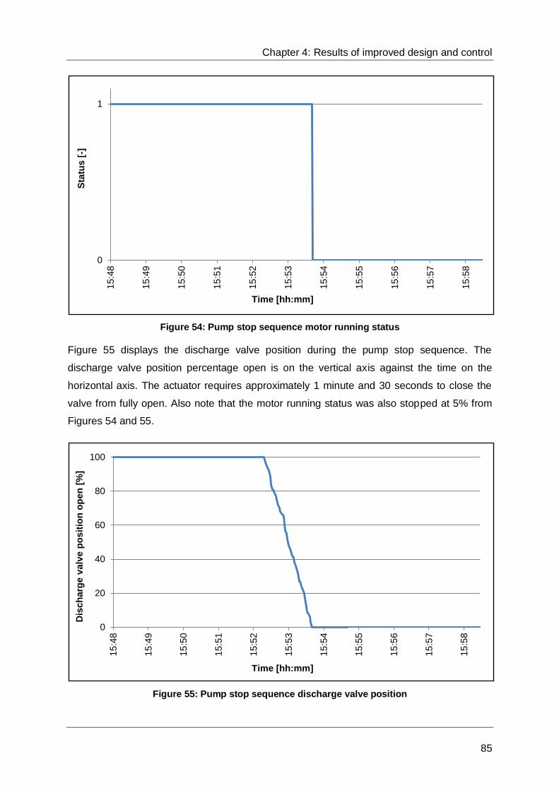
Chapter 4: Results of improved design and control
85
Figure 54: Pump stop sequence motor running status
Figure 55 displays the discharge valve position during the pump stop sequence. The
discharge valve position percentage open is on the vertical axis against the time on the
horizontal axis. The actuator requires approximately 1 minute and 30 seconds to close the
valve from fully open. Also note that the motor running status was also stopped at 5% from
Figures 54 and 55.
Figure 55: Pump stop sequence discharge valve position
0
11
5:4
8
15
:49
15
:50
15
:51
15
:52
15
:53
15
:54
15
:55
15
:56
15
:57
15
:58
Sta
tus
[-]
Time [hh:mm]
0
20
40
60
80
100
15
:48
15
:49
15
:50
15
:51
15
:52
15
:53
15
:54
15
:55
15
:56
15
:57
15
:58
Dis
ch
arg
e v
alv
e p
os
itio
n o
pe
n [
%]
Time [hh:mm]

Chapter 4: Results of improved design and control
86
Figure 56 displays the pump flow during the stop sequence. The flow is on the vertical axis
against the time on the horizontal axis. The closing discharge valves only started to influence
the flow delivered when the valve had reached 15%. At 5% when the motor was stopped,
the flow was reduced to 87.09 l/s. This limited the amount of water hammer in the system.
Figure 56: Pump stop sequence flow
Figure 57 displays the pump and motor bearing temperatures during the stop sequence. The
temperature is on the vertical axis against the time on the horizontal. The bearings tend to
cool as soon as the motor is stopped. The pump DE temperature trend does however differ
from the other bearings. In the bearing daily profile, Figure 49, the temperature of the same
bearing acted irregularly compared to the others. It is expected that the bearing was
damaged.
0
20
40
60
80
100
120
140
160
180
15
:48
15
:49
15
:50
15
:51
15
:52
15
:53
15
:54
15
:55
15
:56
15
:57
15
:58
Flo
w [
l/s
]
Time [hh:mm]

Chapter 4: Results of improved design and control
87
Figure 57: Pump and motor stop sequence bearing temperatures
Figure 58 displays the motor winding temperatures during the stop sequence. The
temperature is on the vertical axis against the time. The windings start to cool when the
motor is stopped.
Figure 58: Motor stop sequence winding temperature
Figure 59 displays the pump and motor DE bearing vibrations during the stop sequence. The
vibration velocity is on the vertical axis against the time on the horizontal axis. The increase
of vibration on the bearings during the stop sequence is an indication of a damaged bearing.
This can be the same pump DE bearing with the temperature rise.
54
56
58
60
62
64
66
68
70
72
74
15
:48
15
:49
15
:50
15
:51
15
:52
15
:53
15
:54
15
:55
15
:56
15
:57
15
:58
Tem
pe
ratu
re [ C
]
Time [hh:mm]
Motor DE Motor NDE Pump DE Pump NDE
61
62
63
64
65
66
67
68
69
70
71
72
15
:48
15
:49
15
:50
15
:51
15
:52
15
:53
15
:54
15
:55
15
:56
15
:57
15
:58
Te
mp
era
ture
[ C
]
Time [hh:mm]
Motor winding U Motor winding V Motor winding W

Chapter 4: Results of improved design and control
88
Figure 59: Pump and motor stop sequence DE bearing vibration
Figure 60 displays the balance disc flow during the stop sequence. The flow is on the vertical
axis against the time on the horizontal axis. The balance disc flow increases when the
discharge valve closes. This is a result of the pressure increase at the discharge.
Figure 60: Pump stop sequence balance disc flow
Figure 61 displays the suction and discharge pressure during the stop sequence. The
pressure is on the vertical axes against the time on the horizontal. Both the suction and
discharge pressure increase when the valve starts to close. The discharge pressure tends to
be equal to the suction pressure when the motor stops.
0
0.5
1
1.5
2
2.5
3
3.5
4
15
:48
15
:49
15
:50
15
:51
15
:52
15
:53
15
:54
15
:55
15
:56
15
:57
15
:58
Velo
cit
y [
mm
/s]
Time [hh:mm]
Motor DE bearing vibration Pump DE bearing vibration
0
0.5
1
1.5
2
2.5
3
3.5
15
:48
15
:49
15
:50
15
:51
15
:52
15
:53
15
:54
15
:55
15
:56
15
:57
15
:58
00
:00
Flo
w [
l/s]
Time [hh:mm]

Chapter 4: Results of improved design and control
89
Figure 61: Pump stop sequence suction and discharge pressure
Figure 62 displays the suction, discharge and balance flow temperature during the stop
sequence. The temperature is on the vertical axis against the time on the horizontal axis.
The balance disc flow temperature decreases when the motor is stopped. The discharge
temperature remains constant. The suction temperature starts to increase when the valve
reaches 5% open.
Figure 62: Pump stop sequence suction, discharge and balance disc flow temperatures
0
1
2
3
4
5
6
7
8
9
10
470
471
472
473
474
475
476
477
478
479
480
15
:48
15
:49
15
:50
15
:51
15
:52
15
:53
15
:54
15
:55
15
:56
15
:57
15
:58
Pre
ss
ure
[M
pa
]
Pre
ss
ure
[k
Pa
]
Time [hh:mm]
Suction Discharge
29
30
31
32
33
34
35
15
:48
15
:49
15
:50
15
:51
15
:52
15
:53
15
:54
15
:55
15
:56
15
:57
15
:58
Tem
pera
ture
[ C
]
Time [hh:mm]
Suction Discharge Balance disc flow

Chapter 4: Results of improved design and control
90
Figure 63 displays the suction temperature and valve position during the stop sequence. The
temperature and discharge valve open percentage are on the vertical axes and the time on
the horizontal axis.
Figure 63: Pump stop sequence suction temperature
The suction temperature increases when the discharge valve closes. This is due to the low
flow through the pump. If the pump continues to run with low flow, this temperature will
increase until the trip temperature is reached. The PLC will then initiate the trip sequence,
protecting the pump from failing from overheating and cavitation.
4.4. Real-time pump control results
The results of the pump statuses were used to determine if the real-time pump scheduling
performed a load shift successfully. The pump schedule, different control philosophies and
interlocks results are examined.
4.4.1. 3-CPFS incorporation
Figure 64 displays the pump and pause status of the 3-CPFS. The alteration between the
statuses is due to the chilled water available on surface. The 3-CPFS statuses have a direct
impact on the control philosophy of IPCM.
0
20
40
60
80
100
29
29.1
29.2
29.3
29.4
29.5
29.6
29.7
29.8
29.9
30
15
:48
15
:49
15
:50
15
:51
15
:52
15
:53
15
:54
15
:55
15
:56
15
:57
15
:58
Dis
ch
arg
e v
alv
e p
os
itio
n o
pe
n [
%]
Te
mp
era
ture
[ C
]
Time [hh:mm]
Suction Valve postion
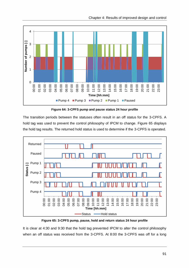
Chapter 4: Results of improved design and control
91
Figure 64: 3-CPFS pump and pause status 24 hour profile
The transition periods between the statuses often result in an off status for the 3-CPFS. A
hold tag was used to prevent the control philosophy of IPCM to change. Figure 65 displays
the hold tag results. The returned hold status is used to determine if the 3-CPFS is operated.
Figure 65: 3-CPFS pump, pause, hold and return status 24 hour profile
It is clear at 4:30 and 9:30 that the hold tag prevented IPCM to alter the control philosophy
when an off status was received from the 3-CPFS. At 8:00 the 3-CPFS was off for a long
0
1
2
3
400
:00
01
:00
02
:00
03
:00
04
:00
05
:00
06
:00
07
:00
08
:00
09
:00
10
:00
11
:00
12
:00
13
:00
14
:00
15
:00
16
:00
17
:00
18
:00
19
:00
20
:00
21
:00
22
:00
23
:00
Nu
mb
er
of
pu
mp
s [
-]
Time [hh:mm]
Pump 4 Pump 3 Pump 2 Pump 1 Paused
Pump 4
Pump 3
Pump 2
Pump 1
Paused
Returned
00
:00
01
:00
02
:00
03
:00
04
:00
05
:00
06
:00
07
:00
08
:00
09
:00
10
:00
11
:00
12
:00
13
:00
14
:00
15
:00
16
:00
17
:00
18
:00
19
:00
20
:00
21
:00
22
:00
23
:00
Sta
tus [
-]
Time [hh:mm]
Status Hold status

Chapter 4: Results of improved design and control
92
enough period to change the control philosophy. The hold tag was found functional for this
purpose.
4.4.2. Pump chamber control
The different control philosophies of each pump chamber resulted in different pump
schedules. The control philosophies incorporated the minimum and maximum dam levels for
each pump chamber. The pump offsets ensured that the dam levels were controlled within
the limits and to create enough dam capacity to perform a load shift.
Figure 66 displays the schedule, maximum number of pumps and dam level of IPCM. The
maximum number of pumps was limited according to the control philosophy when the hold
running status was received. From 8:00 to 9:40 when the hold status was off, the scheduler
could have scheduled the maximum number of pumps if required.
Figure 66: IPCM schedule, maximum number of pumps and dam level 24 hour profile
To ensure the maximum potential of the 3-CPFS is harvested, the maximum number of
pumps is limited to the number of pumps running on Level-22 when the 3-CPFS is running.
This is to prevent the pumps from draining the dam and limit of the 3-CPFS. This is seen at
4:30, 7:00, 10:00, 11:30 and 20:20. At 17:00 the number of pumps was zero on Level-22, but
the schedule of IPCM continued at two until the 15% bottom stable of IPCM was less than
95%, actually 80%. This is an additional safety measure to ensure the dam levels are
controlled within safe limits.
0
10
20
30
40
50
60
70
80
90
100
0
1
2
3
4
00
:00
01
:00
02
:00
03
:00
04
:00
05
:00
06
:00
07
:00
08
:00
09
:00
10
:00
11
:00
12
:00
13
:00
14
:00
15
:00
16
:00
17
:00
18
:00
19
:00
20
:00
21
:00
22
:00
23
:00
Da
m l
ev
el [%
]
Nu
mb
er
of
pu
mp
s [
-]
Time [hh:mm]Schedule Maximum number of pumps Dam level

Chapter 4: Results of improved design and control
93
Figure 67 displays the schedule, maximum number of pumps and dam level of Level-22.
According to the control philosophy, the maximum number of pumps must be limited when
the 15% bottom stable value of IPCM exceeds 90% to prevent flooding. This is shown from
0:00 to 2:30, 15:15 to 18:00 and 22:30 to 24:00. The maximum number of pumps is
increased when the stable value is less than 90%, resulting that the actual dam level has to
be less than 75%.
Figure 67: Level-22 schedule, maximum number of pumps and dam level 24 hour profile
The schedule, maximum number of pumps and dam level of IPCS main are displayed in
Figure 68. A load shift was still possible with only 40% of the dam capacity available in which
to control. This was achievable because the only inflow was from the pumps of Level-46. If
the pumps on Level-46 were off, the dam level remained constant.
0
10
20
30
40
50
60
70
80
90
100
0
1
2
3
4
00
:00
01
:00
02
:00
03
:00
04
:00
05
:00
06
:00
07
:00
08
:00
09
:00
10
:00
11
:00
12
:00
13
:00
14
:00
15
:00
16
:00
17
:00
18
:00
19
:00
20
:00
21
:00
22
:00
23
:00
Dam
lev
el [%
]
Nu
mb
er
of
pu
mp
s [
-]
Time [hh:mm]Schedule Maximum number of pumps Dam level

Chapter 4: Results of improved design and control
94
Figure 68: IPCS schedule, maximum number of pumps and dam level 24 hour profile
Figure 69 displays the schedule, maximum number of pumps and dam level of Level-46. The
maximum available dam capacity is required before the peak periods to accommodate the
inflow from the settlers. The control philosophy made it possible to stop all the pumps in both
peak periods.
Figure 69: Level-46 schedule, maximum number of pumps and dam level 24 hour profile
0
10
20
30
40
50
60
70
80
90
100
0
1
2
3
40
0:0
0
01
:00
02
:00
03
:00
04
:00
05
:00
06
:00
07
:00
08
:00
09
:00
10
:00
11
:00
12
:00
13
:00
14
:00
15
:00
16
:00
17
:00
18
:00
19
:00
20
:00
21
:00
22
:00
23
:00
Da
m l
ev
el [%
]
Nu
mb
er
of
pu
mp
s [
-]
Time [hh:mm]Schedule Maximum number of pumps Dam level
0
10
20
30
40
50
60
70
80
90
100
0
1
2
3
4
00
:00
01
:00
02
:00
03
:00
04
:00
05
:00
06
:00
07
:00
08
:00
09
:00
10
:00
11
:00
12
:00
13
:00
14
:00
15
:00
16
:00
17
:00
18
:00
19
:00
20
:00
21
:00
22
:00
23
:00
Dam
lev
el [%
]
Nu
mb
er
of
pu
mp
s [
-]
Time [hh:mm]Schedule Maximum number of pumps Dam level

Chapter 4: Results of improved design and control
95
4.4.3. Electricity cost savings
The results of pump schedules for a 24-hour profiles illustrated that each level control
philosophies made load shifting possible. The electricity consumption of all the pumps have
to be included in the electricity cost saving calculation.
A baseline of the pump power was established before the project was implemented. This
was used to determine the amount of load shifted out of the peak period. The baseline was
determined from a three month period to ensure it was an accurate reflection of the pump
power consumption.
A load shift project is energy neutral. This implies that the total power consumption of the
measured profile and the baseline have to be equal. Due to the daily variation in the amount
of water pumped, the baseline has to be scaled according to the total power consumed per
day. Figure 70 displays the total power consumption for the same day as the schedule
graphs, baseline and the scaled baseline for the relevant day.
Figure 70: Total power consumption of pumps, baseline and scaled baseline
The daily electricity cost saving is calculated from the hourly difference between the actual
power consumption and the scaled baseline. This difference is then multiplied by the ToU
electricity price structure. Table 13 displays the values of the total power, baseline, scaled
baseline, ToU electricity tariff structure for summer and winter weekday and the total
electricity cost savings. The tariff is determined according to the 2014/2015 Megaflex tariff in
0
3000
6000
9000
12000
15000
18000
21000
00
:00
01
:00
02
:00
03
:00
04
:00
05
:00
06
:00
07
:00
08
:00
09
:00
10
:00
11
:00
12
:00
13
:00
14
:00
15
:00
16
:00
17
:00
18
:00
19
:00
20
:00
21
:00
22
:00
23
:00
Po
we
r [k
W]
Time [hh:mm]
Power consumption Baseline Scaled baseline
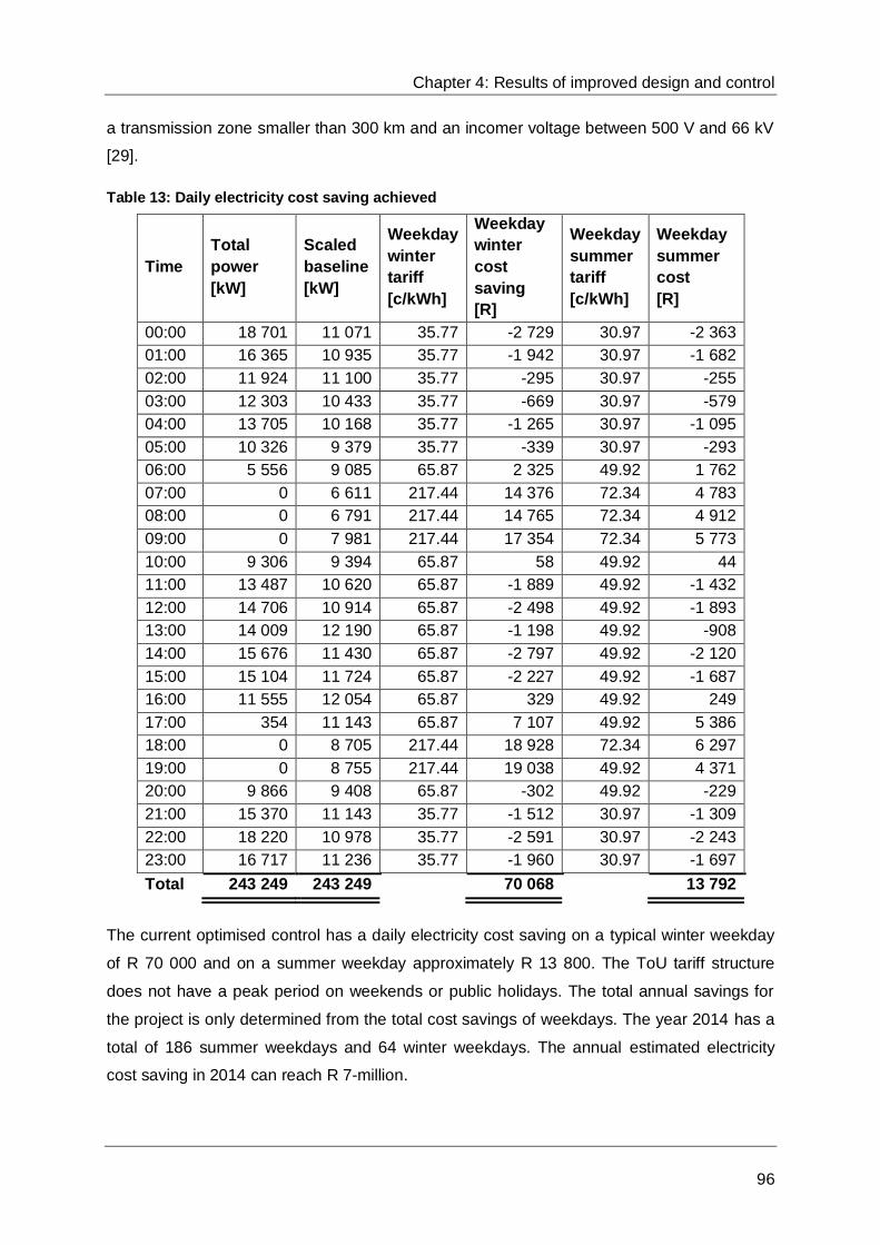
Chapter 4: Results of improved design and control
96
a transmission zone smaller than 300 km and an incomer voltage between 500 V and 66 kV
[29].
Table 13: Daily electricity cost saving achieved
Time
Total
power
[kW]
Scaled
baseline
[kW]
Weekday
winter
tariff
[c/kWh]
Weekday
winter
cost
saving
[R]
Weekday
summer
tariff
[c/kWh]
Weekday
summer
cost
[R]
00:00 18 701 11 071 35.77 -2 729 30.97 -2 363
01:00 16 365 10 935 35.77 -1 942 30.97 -1 682
02:00 11 924 11 100 35.77 -295 30.97 -255
03:00 12 303 10 433 35.77 -669 30.97 -579
04:00 13 705 10 168 35.77 -1 265 30.97 -1 095
05:00 10 326 9 379 35.77 -339 30.97 -293
06:00 5 556 9 085 65.87 2 325 49.92 1 762
07:00 0 6 611 217.44 14 376 72.34 4 783
08:00 0 6 791 217.44 14 765 72.34 4 912
09:00 0 7 981 217.44 17 354 72.34 5 773
10:00 9 306 9 394 65.87 58 49.92 44
11:00 13 487 10 620 65.87 -1 889 49.92 -1 432
12:00 14 706 10 914 65.87 -2 498 49.92 -1 893
13:00 14 009 12 190 65.87 -1 198 49.92 -908
14:00 15 676 11 430 65.87 -2 797 49.92 -2 120
15:00 15 104 11 724 65.87 -2 227 49.92 -1 687
16:00 11 555 12 054 65.87 329 49.92 249
17:00 354 11 143 65.87 7 107 49.92 5 386
18:00 0 8 705 217.44 18 928 72.34 6 297
19:00 0 8 755 217.44 19 038 49.92 4 371
20:00 9 866 9 408 65.87 -302 49.92 -229
21:00 15 370 11 143 35.77 -1 512 30.97 -1 309
22:00 18 220 10 978 35.77 -2 591 30.97 -2 243
23:00 16 717 11 236 35.77 -1 960 30.97 -1 697
Total 243 249 243 249 70 068 13 792
The current optimised control has a daily electricity cost saving on a typical winter weekday
of R 70 000 and on a summer weekday approximately R 13 800. The ToU tariff structure
does not have a peak period on weekends or public holidays. The total annual savings for
the project is only determined from the total cost savings of weekdays. The year 2014 has a
total of 186 summer weekdays and 64 winter weekdays. The annual estimated electricity
cost saving in 2014 can reach R 7-million.

Chapter 4: Results of improved design and control
97
The actual savings achieved for the project for the year 2014 is displayed in Table 14. The
minimum saving achieved was used for the outstanding months of the year. The control
schedule was only followed from February. The total electricity cost saving for the year 2014
achieved and predicted at about R 6-million.
Table 14: Savings achieved and minimum saving predicted in 2014
Month in 2014
Electricity cost
saving
[R]
Load shifted from
peak period
[MW]
January 0 0.00
February 233 951 8.05
March 279 248 8.49
April 252 709 8.04
May 224 687 5.86
June 1 241 916 7.12
July 1 340 384 6.18
August 1 451 128 7.79
September (Minimum saving achieved) 224 687 5.86
October (Minimum saving achieved) 224 687 5.86
November (Minimum saving achieved) 224 687 5.86
December (Minimum saving achieved) 224 687 5.86
Total 5 922 711
The estimated electricity cost savings reached 85% of the maximum savings. Bearing in
mind that the projected savings were set to the minimum and in January no load shift was
performed. The average load shifted from the peak period was 6.82 MW, and the target for
the project was 5.58 MW.
4.5. Real-time efficiency results
The real-time pump efficiency results of the pump were found to be higher than the
maximum efficiency the pump manufacturers specify. A daily running average efficiency of
84.06% was calculated when observing an individual pump. The maximum efficiency for a
multistage centrifugal pump is 83%. Figure 71 displays the 24-hour profile for the efficiency
of a pump using Equation 3.14 and the installed instrumentation.
The efficiency can only be calculated when the pump is running. Zero efficiency was
returned when the pump was off. It is evident from the graph that an efficiency of 84% is
returned from the equation.

Chapter 4: Results of improved design and control
98
Figure 71: Pump efficiency calculated with differential temperature and pressure
The unrealistic efficiency obtained from the differential temperature led to an investigation.
The system was designed for two pumps to transfer water in one column. Each of the
dewatering columns had a flow meter installed. This resulted that Equation 3.13 could be
used to verify the efficiency results obtained. The static head was known, the flow could be
used when only one pump per column was running and the power was measured. Figure 72
displays the pump efficiency verified with the static head, flow and power efficiency.
Figure 72: Pump efficiency verified with static head, flow and power efficiency
0
10
20
30
40
50
60
70
80
90
100
00
:00
01
:00
02
:00
03
:00
04
:00
05
:00
06
:00
07
:00
08
:00
09
:00
10
:00
11
:00
12
:00
13
:00
14
:00
15
:00
16
:00
17
:00
18
:00
19
:00
20
:00
21
:00
22
:00
23
:00
Eff
icie
ncy [
%]
Time [hh:mm]
Differential temperature and pressure (Eq. 3.14)
0
10
20
30
40
50
60
70
80
90
100
00
:00
01
:00
02
:00
03
:00
04
:00
05
:00
06
:00
07
:00
08
:00
09
:00
10
:00
11
:00
12
:00
13
:00
14
:00
15
:00
16
:00
17
:00
18
:00
19
:00
20
:00
21
:00
22
:00
23
:00
Eff
icie
ncy [
%]
Time [hh:mm]
Differential temperature and pressure (Eq. 3.14) Static head, flow and power (Eq. 3.13)

Chapter 4: Results of improved design and control
99
Similar to Figure 71, zero efficiency was returned when the pump was not running. Zero
efficiency was also returned during the period from 14:30 to 17:15. The second pump in the
same column was also operated in this period. This resulted in that the flow of the pump
could not be obtained. The average daily efficiency of the static head, flow and power is
72.81%.
The static head in the previous efficiency calculation is used to determine the pressure of the
fluid required. This enabled verification of installed pressure sensors. The static head
pressure can be substituted with the measured pressure in Equation 3.13. Figure 73
displays the efficiency determined from the pressure sensors, flow and power.
Figure 73: Pressure sensors verified with pump efficiency
It is clear that the data received from the pressure sensors were correct if compared to the
static head. The average daily efficiency using the differential pressure, flow and power is
71.82%. The difference between the static head and pressure sensor results is 1.01%.
The last method to verify the efficiency results was to use the result of the current installed
efficiency system. The efficiencies of the pumps were reported on a monthly basis. The
efficiency of the specific pump was 74%. Figure 74 displays the efficiencies verified with the
installed system efficiency compared to the other efficiency results.
0
10
20
30
40
50
60
70
80
90
100
00
:00
01
:00
02
:00
03
:00
04
:00
05
:00
06
:00
07
:00
08
:00
09
:00
10
:00
11
:00
12
:00
13
:00
14
:00
15
:00
16
:00
17
:00
18
:00
19
:00
20
:00
21
:00
22
:00
23
:00
Eff
icie
ncy [
%]
Time [hh:mm]Differential temperature and pressure (Eq. 3.14) Static head, flow and power (Eq. 3.13)
Differential pressure, flow and power (Eq. 3.13)

Chapter 4: Results of improved design and control
100
Figure 74: Pump efficiency verified with the installed system
The efficiency calculated with Equation 3.14 is a function of the differential temperature,
pressure and the thermodynamic properties. From Figures 72 to 74 it is evident that the
pressure sensors are correct. The thermodynamic properties are determined from a
thermodynamic table. This leaves the differential temperature to be the only parameter being
incorrect.
The specification sheets from the manufacturers show that a 3-wire PT1000 temperature
probe has a tolerance of ±(0.30+0.005 |t|); |t| is the measured temperature [89]. The
operating temperature of the temperature probes range from 26°C to 30°C. The average
tolerance that can be expected is 0.44°C per temperature probe.
It was determined that a value of 0.31546°C must be added to the differential temperature in
Equation 3.14 to give the same daily average of 74.0%. This adjustment is within the
tolerance of the installed temperature probes. The results of the adjusted temperature are
shown in Figure 75.
0
10
20
30
40
50
60
70
80
90
100
00
:00
01
:00
02
:00
03
:00
04
:00
05
:00
06
:00
07
:00
08
:00
09
:00
10
:00
11
:00
12
:00
13
:00
14
:00
15
:00
16
:00
17
:00
18
:00
19
:00
20
:00
21
:00
22
:00
23
:00
Eff
icie
ncy [
%]
Time [hh:mm]
Differential temperature and pressure (Eq. 3.14) Static head, flow and power (Eq. 3.13)
Differential pressure, flow and power (Eq. 3.13) Installed system
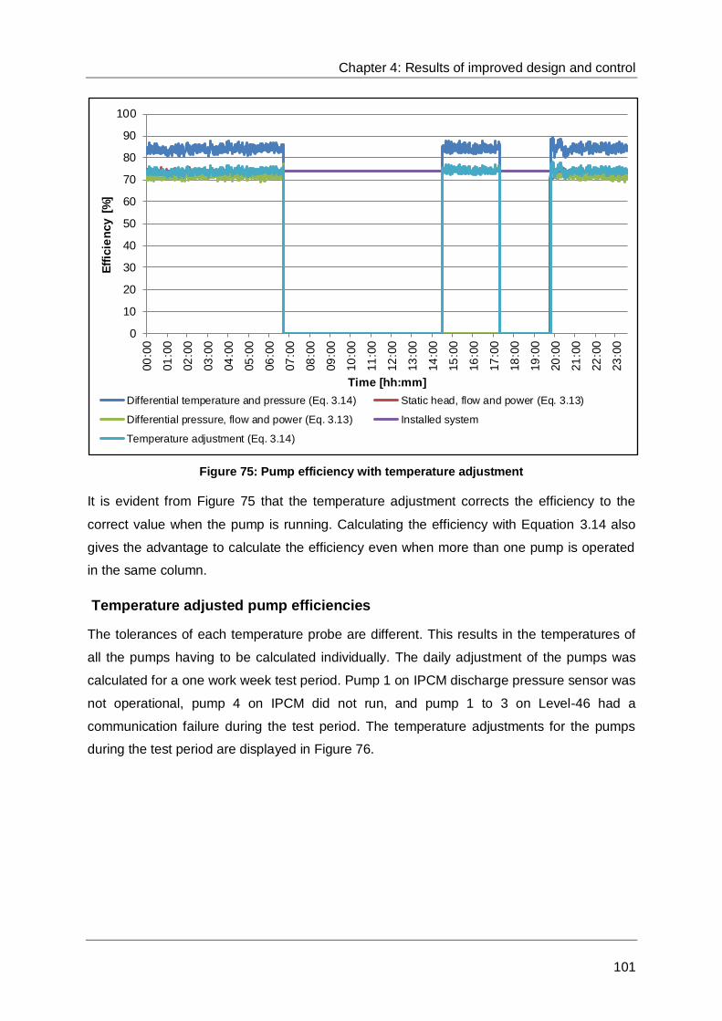
Chapter 4: Results of improved design and control
101
Figure 75: Pump efficiency with temperature adjustment
It is evident from Figure 75 that the temperature adjustment corrects the efficiency to the
correct value when the pump is running. Calculating the efficiency with Equation 3.14 also
gives the advantage to calculate the efficiency even when more than one pump is operated
in the same column.
Temperature adjusted pump efficiencies
The tolerances of each temperature probe are different. This results in the temperatures of
all the pumps having to be calculated individually. The daily adjustment of the pumps was
calculated for a one work week test period. Pump 1 on IPCM discharge pressure sensor was
not operational, pump 4 on IPCM did not run, and pump 1 to 3 on Level-46 had a
communication failure during the test period. The temperature adjustments for the pumps
during the test period are displayed in Figure 76.
0
10
20
30
40
50
60
70
80
90
100
00
:00
01
:00
02
:00
03
:00
04
:00
05
:00
06
:00
07
:00
08
:00
09
:00
10
:00
11
:00
12
:00
13
:00
14
:00
15
:00
16
:00
17
:00
18
:00
19
:00
20
:00
21
:00
22
:00
23
:00
Eff
icie
ncy [
%]
Time [hh:mm]
Differential temperature and pressure (Eq. 3.14) Static head, flow and power (Eq. 3.13)
Differential pressure, flow and power (Eq. 3.13) Installed system
Temperature adjustment (Eq. 3.14)

Chapter 4: Results of improved design and control
102
Figure 76: Daily temperature adjustments for the efficiencies
The installed temperature probes have a specified tolerance of ±0.44°C. This implies that the
maximum temperature adjustment can be up to 0.88°C. The maximum is possible if the
suction temperature probe is -0.44°C and the discharge temperature probe is +0.44°C. The
temperature adjustments in Figure 76 are within the maximum tolerance of the temperature
probes.
The temperature adjustment was set to the average of the adjusted temperature during the
test period. The results of the temperature adjusted efficiencies are displayed in Table 15.
Table 15: Temperature adjusted pump efficiency results
Pump
chamber
Pump
number
Installed
system
efficiency
[%]
Eq. 3.14
efficiency
[%]
Temperature
adjustment
[°C]
Eq. 3.14
temperature
adjusted
efficiency
[%]
Deviation
between
installed
and
adjusted
efficiency
IPC
M
1 79.00 Discharge pressure sensor failure.
2 74.00 67.78 -0.25 73.12 0.88
3 72.00 72.39 0.02 71.82 0.18
4 70.00 Pump not operated during test period.
Le
ve
l-22 1 74.00 84.07 0.33 73.56 0.44
2 66.00 70.59 0.18 66.37 -0.37
3 69.00 84.38 0.53 68.71 0.29
4 71.00 74.16 0.14 70.48 0.52
-0.30
-0.20
-0.10
0.00
0.10
0.20
0.30
0.40
0.50
0.60
1 2 3 4 1 2 3 4 1 2 3 4 1 2 3 4
IPCM L22 IPCS L46
Te
mp
era
ture
ad
just
me
nt
[ C
]
Pump number [-]Pump chamber [-]
Monday Tuesday Wednesday Thursday Friday

Chapter 4: Results of improved design and control
103
Table 15 (continue): Temperature adjusted pump efficiency results
Pump
chamber
Pump
number
Installed
system
efficiency
[%]
Eq. 3.14
efficiency
[%]
Temperature
adjustment
[°C]
Eq. 3.14
temperature
adjusted
efficiency
[%]
Deviation
between
installed
and
adjusted
efficiency
IPC
S
1 74.00 84.62 0.32 74.12 -0.12
2 70.00 81.77 0.40 70.13 -0.13
3 77.00 77.50 -0.01 77.76 -0.76
4 72.00 76.54 0.05 74.99 -2.99
Le
ve
l-46 1 61.00 Communication failure.
2 70.00 Communication failure.
3 77.00 Communication failure.
4 70.00 77.10 0.28 69.50 0.50
The maximum deviation between the installed system and the temperature adjusted
efficiency is 2.99. The temperature adjustment of the pump in question fluctuated the most in
Figure 76. The temperature probes of the specific pump have to be investigated.
The other pumps have a maximum deviation of 0.88. Efficiencies of pumps are used as a
trend line over a period of time. When a minimum limit is reached or a sudden large
depreciation in the efficiency is present, the pump must be refurbished or replace. The
deviation of 0.88 is in an acceptable range.
Chapter 4: Results of improved design and control
104
4.6. Summary
The data of the installed instrumentation is analysed in this chapter. It is clear that the
installed instrumentation will prevent failure of the pump in normal operating conditions.
The similar failure conditions could not be repeated due to the risk involved. A low flow
scenario was represented when the pump was stopped. The valve closed to 5% when the
pump motor was stopped. This allowed for testing of the additional instrumentation. It was
evident that the suction temperature probe would detect the temperature increase due to the
low flow. The installed instrumentation did not show a condition to trip the pump.
The results of the control philosophy of the pumps showed a noticeable electricity cost
saving. The savings achieved and projected for 2014 was R 6-million. This was achieved
through optimising the control schedule of the pump. The pump load in the expensive peak
periods was reduced. This was achieved through preparing the dam correctly in the less
expensive off-peak and standard periods.
The pump efficiencies were calculated with the additional temperature probes installed. This
allowed calculating the efficiencies of each individual pump in real-time. The efficiencies
were calculated incorrectly. Using the output power over the input power and the installed
system the efficiencies could be verified. The temperature sensors were found to be correct.
The efficiencies were then adjusted with the temperature to ensure the efficiencies were
calculated correctly.

105
Chapter 5: Conclusion,
recommendations and research
opportunities
In this chapter a conclusion on the results obtained is made. The results also make it
possible to suggest alterations to the project. From this study several opportunities for
further studies are identified. These opportunities are also discussed in this chapter.

Chapter 5: Conclusion, recommendations and research opportunities
106
5.1. Conclusion
This study focused on the automation and control of mine dewatering systems. A case study
was presented on a project done on a pump dewatering system of the mine. During
implementation a pump failed after it had been automated and commissioned. The
automation of the pump was investigated to protect pumps from failing in similar operating
conditions.
From the literature study it is explained which condition of a pump must be monitored to
prevent failure. The instrumentation according to the current best practice was found
mandatory for pump automation. This can be seen from the results of the installed
instrumentation displayed for a daily operating profile. It is evident from the operating profiles
that the installed instrumentation will prevent failure from the conditions they were intended
to monitor.
The connection between the shoeblock and the discharge valve failed during the start-up
sequence. This resulted in a period of low flow which caused a temperature increase and
cavitation in the pump. The installed instrumentation was not able to detect the abnormal
operating conditions.
The failure of the automated pump proved additional precautions must be taken to prevent
similar failure. The intricate investigation of the pump failure made it possible to identify the
root cause of failure. This made it possible to make the following improvements to the
current best practice:
1. Equalising differential pressure across the discharge valve through opening it to 10%
every 30 minutes when the pump is not running.
2. Redesigning the shoeblock connection to increase the force it can transfer.
3. Additional temperature probes were installed to measure the temperature increase
of the water across the pump.
4. Setting of an under torque limit on the actuator to ensure the gate is opening.
5. Locking the flow switch to prevent unauthorised personnel from lowering the trip
limit.
The control of the automated dewatering system proved to be feasible. Informed control
decisions could be made through interlocking all the control parameters from a centralised
system. This was made possible with the automation of the pumps and including the dam
levels and 3-CPFS status. The pump control graphs illustrate the dam levels remained in the
safe specified ranges.

Chapter 5: Conclusion, recommendations and research opportunities
107
The total electricity cost saving for the year 2014 achieved and predicted is R 6-million
through minimising pumping in the peak periods. This is more than half of the total
automation cost. This proves that in a period of two years the initial automation cost will have
been repaid with savings from electricity usage. The control also included the running status
of the installed 3-CPFS. This ensures that the maximum potential of the 3-CPFS is
harvested and the pump load is shifted safely.
The savings were calculated, using the pump running status only. Additional savings were
achieved with the 3-CPFS that was not included in these savings. The control of the dam
schedules ensured that the operation 3-CPFS was increased. The dam levels were prepared
correctly to ensure the maximum potential of the 3-CPFS was realised.
The installed instrumentation did make it possible to calculate the pump efficiencies. The
suction and discharge pressure sensors were used to determine the total head each pump
developed. The additional suction and discharge temperature probes were used to
determine the temperature increase across the pump. A formula found in the literature
derived from Thermodynamic principles was used to calculate the efficiency. The increase of
temperature is an indication of efficiency losses.
This allowed calculating the efficiency of each individual pump when it was operated. The
efficiencies were verified by comparing the power input with the power output and the
current installed efficiency system. The temperature was adjusted and the efficiencies were
within 5% of the verified efficiencies.
Three aspects of the dewatering system were investigated in this study. All three were
proved to be successful within an acceptable range. Additional instrumentation was added
according to the best practice to automate a pump system to improve the reliability. This
allowed for safe control from the surface to realise electricity cost savings.

Chapter 5: Conclusion, recommendations and research opportunities
108
5.2. Recommendations
It is recommended that automated pumps must include the best practice instrumentation as
discussed in this study. The conditions they monitored must be interlocked according to the
manufacturer. If the operating conditions are less, the limits can be reduced to initiate the
stop sequence at an earlier stage.
The pressure across the discharge valve must be equalised when there is a possibility for a
differential pressure. This will prevent the pressure from holding the gate in the closed
position resulting in additional forces to be applied. The pressure equalising can be easily
performed through altering the control software.
Refurbishment of equipment is usually less expensive than replacing it with new equipment.
When equipment is refurbished, it is recommended to ensure it meets the original design
specifications. If the specifications are not met, design improvements must be made. It is
also recommended to improve the connection, between the shoeblock and spindle, of
refurbished gate valves to prevent failure.
The additional temperature probes to measure the temperature increase across the pump is
recommended for pump automation. The redundancy of the automation is increased from
protecting the pump against low flow. This is achieved when multiple instruments monitor the
same condition. If one of the instruments fails, the other one will still initiate the trip
sequence.
All involved personnel must approve and document the limits and control ranges of the
instrumentation. These limits and control ranges must be verified and locked during
commissioning. Only authorised personnel should be able to change the limits to ensure
safe operation of the pumps.
It is recommended to control an automated dewatering system from a centralised system. All
the required data for the systems involved must be displayed or be available. This allows the
operator or system to make an informed control decision from an overview of the entire
system. It is possible to achieve noticeable electricity cost savings if a ToU tariff structure is
used for electricity.
Real-time pump efficiency can be determined from the head developed and temperature rise
across the pump. This can assist in calculating the efficiencies of pumps sharing a common
column with only one flow meter.
Chapter 5: Conclusion, recommendations and research opportunities
109
5.3. Research opportunities
The improved control schedule of the dewatering system results in increased switching of
the pump. This increases the maintenance cost of the pumps. It is also suspected that the
increased switching will increase the rate at which the pump efficiencies deteriorate. The
real-time efficiency calculation allows for the opportunity to examine the effect the switching
of pumps has on the pump efficiencies.
The pumps were scheduled to run the most efficient pumps during the peak and standard
periods first. The least efficient pumps would start first during the off-peak periods. This can
realise an additional electricity cost saving. The additional electricity cost saving from
prioritising the pumps according to their efficiencies can be verified.

110
Bibliography
[1] S. Walker, “The pump-makers' perpective,” Engineering & Mining Journal, vol. 214, no.
11, pp. 50-54, November 2013.
[2] W. Schoeman, “The integrated effect of DSM on mine chilled water systems,” M.Eng
dissertation, North-West University, Potchefstroom, 2014.
[3] X. Zhang, L. Gao, D. Barrett and Y. Chen, “Evaluating water management practice for
sustainable mining,” Water, vol. 6, no. 2, pp. 414-433, February 2014.
[4] S. Thein, “Demand side management on an intricate multi-shaft pumping system from a
single point of control,” M.Eng dissertation, North-West University, Potchefstroom, 2007.
[5] R. W. Gaikwad, “Review and research needs of active treatment of acid mine drainage
by ion exchange,” Electronic Journal of Environmental, Agricultural and Food Chemistry,
vol. 9, no. 8, pp. 1343-1350, 2010.
[6] K. Farhadi, A. Bousbia-salah and F. D'Auria, “A model for the analysis of pump start-up
transients in Tehran Research Reactor,” Progress in Nuclear Energy, vol. 49, no. 7, pp.
499-510, September 2007.
[7] D. Stephenson, “Distribution of water in deep gold mines,” International Journal of Mine
Water, vol. 2, no. 2, pp. 21-30, 1983.
[8] D. A. J. Ross-Watt, “Presidential address: mining engineering - a discipline for the
future,” Journal of the South African Institute of Mining and Metallurgy, vol. 95, no. 6, pp.
241-268, 1995.
[9] A. Prinsloo, “Energy cost optimisation of a complex mine pumping system,” M.Eng
dissertation, North-West University, Potchefstroom, 2004.
[10] R. W. Wilson and A. Pieters, “Design and construction of a surface air cooling and
refrigeration installation at a South African mine,” in 12th US/North American mine
ventilation symposium, Reno, 2008.
Bibliography
111
[11] D. J. Stanton, “Development and testing of an underground remote refrigeration plant,”
M.Eng dissertation, North-West University, Potchefstroom, 2003.
[12] J. Van der Walt and A. Whillier, “Considerations in the design of integrated systems for
distributing refrigeration in deep mines,” Journal of the South African Institute of Mining
and Metallurgy, vol. 94, no. 3, pp. 109-124, 1994.
[13] M. Biffi and D. J. Stanton, “Cooling power for a new age,” in Third International
Conference "Platinum in Transformation", Rustenburg, 2008.
[14] A. Botha, “Optimising the demand of a mine water reticulation system to reduce
electricity consumption,” M.Eng dissertation, North-West University, Potchefstroom,
2010.
[15] J. N. de la Vergne, “Explosives and drilling,” in The Hard Rock Miner's Handbook, North
Bay, McIntosh Engineering, 2003, pp. 209-214.
[16] J. Vosloo, L. Liebenberg and D. Velleman, “Energy savings for a deep-mine water
reticulation system,” Applied Energy, vol. 92, pp. 328-335, April 2012.
[17] G. Van den Berg and R. Cooke, “Hydraulic hoisting technology for platinum mines,”
Journal of the South African Institute of Mining and Metallurgy, vol. 105, no. 5, pp. 323-
332, 2010.
[18] J. N. de la Vergne, “Mine dewatering,” in The Hard Rock Miner's Handbook, North Bay,
McIntosh Engineering, 2003, pp. 187-200.
[19] C. Cilliers, “Cost savings on mine dewatering pumps by reducing preparation- and
comback loads,” M.Eng dissertation, North-West University, Potchefstroom, 2014.
[20] J. Hall, “Process pump control,” Chemical Engineering, vol. 117, no. 12, pp. 30-33,
November 2010.
[21] B. Jafarzadeh, A. Hajari, M. M. Alishahi and M. H. Akbari, “The flow simulation of a low-
specific-speed high-speed centrifugal pump,” Applied Mathematical Modelling, vol. 35,
no. 1, pp. 242-249, 2011.
[22] E. Brito, “Making pump maintenance mandatory,” Chemical Engineering, vol. 118, no.
10, pp. 48-53, October 2011.

Bibliography
112
[23] S. Perju and L. V. Hasegan, “Reducing energy consumption by upgrading pumping
stations in water distribution systems,” Environmentral Engineering & Management
Journal, vol. 12, no. 4, pp. 735-740, April 2013.
[24] J. C. Vosloo, J. Van Rensburg and A. Botha, “Optimising the demand of a mine water
reticulation system to reduce electricy consumption,” in Industrial and Commercial Use
of Energy (ICUE) conference, Cape Town, 2010.
[25] H. J. Van Antwerpen and G. P. Greyvenstein, “Use of turbines for simultaneous
pressure regulation and recovery in secondary cooling water systems in deep mines,”
Energy Conversion and Management, vol. 46, no. 4, pp. 563-575, 2005.
[26] P. Fraser and D. Le Roux, “Three-chamber pump system for DSM,” Energize, vol. 19,
no. 9, pp. 51-54, 2007.
[27] W. Rautenbach, D. L. Krueger and E. H. Matthews, “Reducing the electricity cost of a
three-pipe water pumping system - a case study using software,” Journal of Energy in
Southern Africa, vol. 16, no. 4, pp. 41-47, 2005.
[28] S. Yadav, “Some aspects of performance improvement of Pelton wheel turbine with
reengineered blade and auxiliary,” International Journal of Science and Engineering
Research, vol. 2, no. 9, pp. 2-5, 2011.
[29] Eskom, “Tariff & Charges Booklet,” Eskom, Johannesburg, 2014/15.
[30] B. Barán, C. Von Lücken and A. Sotelo, “Multi-Objective pump scheduling optimisation
using evolutionary strategies,” Advances in Engineering Software, vol. 36, no. 1, pp. 39-
47, 2005.
[31] Y. Tang, G. Zheng and S. Zhang, “Optimal control approaches of pumping station to
achieve efficiency and load shifting,” International Journal of Electrical Power & Energy
Systems, vol. 55, pp. 572-580, 2014.
[32] X. Zhuan and X. Xia, “Optimal operation scheduling of a pumping station with multiple
pumps,” Applied Energy, vol. 104, pp. 250-257, 2013.
[33] J. LePree, “Pump it up,” Chemical Engineering, vol. 118, no. 2, pp. 25-28, June 2011.
Bibliography
113
[34] R. Pelzer, R. P. Richter, M. Kleingeld and J. Van Rensburg, “Performance comparison
between manual and automated DSM pumping projects,” in Industrial and Commercial
Use of Energy (ICUE) conference, Cape Town, 2009.
[35] I. Kougias and N. Theodossiou, “Multi-objective pump scheduling optimization using
harmony search algorithm (HSM) and polyphonic HSA,” Water Resources Management,
vol. 27, no. 5, pp. 1249-1261, 2013.
[36] J. C. Vosloo, “A new minimum cost model for water reticulation systems on deep
mines,” Ph.D thesis, North-West University, Potchefstroom, 2008.
[37] A. Almasi, “Renovation and system upgrades,” World Pumps, vol. 2013, no. 1, pp. 16-
18, January 2013.
[38] R. Beebe, “Optimize time for overhaul of your pumps using condition monitoring,” World
Pumps, vol. 2004, no. 452, pp. 24-28, May 2004.
[39] E. Hoop, “Control valves: an evolution in design,” Chemical Engineering, pp. 48-51,
August 2012.
[40] A. Almasi, “Power plant condition monitoring,” Power Engineering, vol. 115, no. 8, pp.
60-63, August 2011.
[41] A. Almasi, “CPI Machinery: commissioning, startup and piping,” Chemical Engineering,
vol. 119, no. 13, pp. 42-50, December 2012.
[42] A. Almasi, “Condition monitoring for rotating machinery,” Chemical Engineering, vol.
119, no. 3, pp. 55-60, March 2012.
[43] S. K. Chatterjee, “Improve rotary equipment reliability with checklists,” Chemical
Engineering, vol. 120, no. 9, pp. 52-57, September 2013.
[44] S. Shiels, “Optimizing centrifugal pump operation,” World Pumps, vol. 2001, no. 412, pp.
35-39, 2001.
[45] A. Almasi, “Practical notes on component failure,” World Pumps, vol. 2012, no. 10, pp.
40-43, October 2012.
Bibliography
114
[46] A. T. Sayers, “Hydraulic pumps,” in Hyrdaulic and compressible flow turbomachines,
London, McGraw-Hill, 1990, pp. 31-87.
[47] I. Halkijevic, Z. Vukovic and D. Vouk, “Frequency pressure regulation in water supply
systems,” Water Science & Technology: Water Supply, vol. 13, no. 4, pp. 896-905,
2013.
[48] W. Chaiworapuek, J.-Y. Champagne, M. El Haj em and C. Kittichaikan, “An
Investigation of the Water Flow Past the Butterfly Valve,” AIP Conference Proceedings,
vol. 1225, no. 1, pp. 249-262, June 2010.
[49] B. R. Munson, D. F. Young, T. H. Okiishi and W. W. Heubsch, “Viscous flow in pipe,” in
Fundamentals of fluid mechanics, John Wiley & Sons, 2010, pp. 383-460.
[50] J. Tonkin, “Reducing costs in parallel pumping,” World Pumps, vol. 2012, no. 5, pp. 32-
37, May 2012.
[51] S. D. Kyparissis and D. P. Margaris, “Experimental investigation and passive flow
control of a cavitating centrifugal pump,” International Journal of Rotating Machinery,
vol. 2012, pp. 1-8, 2012.
[52] R. Beebe and S. Jankins, “Condition monitoring methods for pumps,” Chemical
Engineering, vol. 119, no. 9, pp. 34-39, September 2012.
[53] G. Rohlfing, “Condition monitoring of multiphase pumps,” World Pumps, vol. 2010, no.
4, pp. 34-39, April 2010.
[54] M. Yates, “Pump performance monitoring complements condition monitoring,” World
Pumps, vol. 2002, no. 428, pp. 36-38, May 2002.
[55] E. W. Wallace, M. White and G. Parks, “Commissioning and start-ups of new units
(pumps),” in The 25th International Pump Users Symposium, Houston, 2009.
[56] R. Beebe, “Pump monitoring: unusual incidents,” World Pumps, vol. 2010, no. 4, pp. 24-
28, April 2010.
[57] A. Budris, “Power precaustions,” WaterWorld, vol. 29, no. 8, pp. 10-13, August 2013.
Bibliography
115
[58] S. Elaoud and E. Hadj-Taïeb, “Influence of pump starting times on transient flows in
pipes,” Nuclear Engineering and Design, vol. 241, no. 9, pp. 3624-3631, September
2011.
[59] R. Birajdar, R. Patil and K. Khanzode, “Vibration and noise in centrifugal pumps -
Sources and diagnosis methods,” in 3rd International Conference on Integrity, Reliability
and Failure, Porto, 2009.
[60] S. K. Chatterjee, “Get the most out of vibration analysis,” Chemical Engineering, vol.
118, no. 1, pp. 36-42, January 2011.
[61] A. Almasi, “Practical vibrational monitoring to identify-damaged, cracked and worn
components in power plants,” Power Engineering, vol. 116, no. 4, pp. 20-26, April 2012.
[62] A. Almasi, “How vibrations can affect condition,” World Pumps, vol. 2013, no. 2, pp. 26-
27, February 2013.
[63] N. R. Sakthivel, V. Sugumaran and S. Babudevasenapati, “Vibration based fault
diagnosis of monoblock centrifugal pump using decision tree,” Expert Systems with
Applications, vol. 37, no. 6, pp. 4040-4049, June 2010.
[64] M. A. Abu-Zeid and S. M. Abdel-Rahman, “Bearing problems' effects on the dynamic
performance of pumping stations,” Alexandria Engineering Journal, vol. 52, no. 3, pp.
241-248, 2013.
[65] A. Almasi, “Thermal analysis for temp apps,” World Pumps, vol. 2013, no. 5, pp. 30-33,
May 2013.
[66] R. Koch, “Remedy to black oil problems in centrifugal pumps with ball bearings,”
Tribology & Lubrication Technology, vol. 60, no. 6, pp. 51-55, June 2004.
[67] R. Arifulin, I. Kashtanov and N. Antonov, “Shut-off device for well-head equipment,”
Chemical & Petroleum Engineering, vol. 48, no. 1/2, pp. 35-39, January 2012.
[68] B.-S. Yang, W.-W. Hwang, M.-H. Ko and S.-J. Lee, “Cavitation detection of butterfly
valve using support vector machines,” Journal of Sound and Vibration, vol. 287, no. 1,
pp. 25-43, 2005.

Bibliography
116
[69] P. Naseradinmousavi and C. Nataraj, “Nonlinear mathematical modeling of butterfly
valves driven by solenoid actuators,” Applied Mathematical Modeling, vol. 35, no. 5, pp.
2324-2335, 2011.
[70] Fisher Controls International, “Valve and actuator types,” in Control Valve Handbook,
Marshalltown, Emerson Process Management, 2005, pp. 41-66.
[71] R. Beebe, “Alternative measures,” Mechanical Engineering, vol. 133, no. 8, pp. 42-43,
August 2011.
[72] M.-J. Chern, P.-H. Hsu, Y.-J. Cheng, P.-Y. Tseng and C.-M. Hu, “Numerical study on
cavitation occurrence in globe valve,” Journal of Energy Engineering, vol. 139, no. 1, pp.
25-34, March 2013.
[73] B. Nesbitt, “Valve selection for process systems,” World Pumps, vol. 425, no. 2, pp. 42-
46, 2002.
[74] T. Bishop, M. Chapeaux, L. Jaffer, K. Nair and S. Patel, “Ease control valve selection,”
Chemical Engineering Progress, vol. 98, no. 11, pp. 52-56, 2002.
[75] V. Ivanov, A. Olienikov, D. Denisevich and B. Pektimirov, “Emergency shut-off valve for
pipelines,” Chemical & Petroleum Engineering, vol. 49, no. 5/6, pp. 400-402, September
2013.
[76] Q. Zuo, S. Qiu, W. Lu, W. Tian, G. Su and Z. Xiao, “Water hammer characteristics of
integral pressurized water reactor primary loop,” Nuclear Engineering and Design, vol.
261, pp. 165-173, August 2013.
[77] W. J. Rahmeyer, H. L. Miller and S. V. Sherikar, “Cavitation testing results for a tortuous
path control valve,” ASME - Publications - FED, vol. 210, pp. 63-68, 1995.
[78] J. Wu, S. Sun and D. Wang, “The new design of globe valve virtual assembly design,”
Advanced Materials Research, no. 926-930, pp. 1623-1626, 2014.
[79] C. C. Tsai, C. Y. Chang and C. H. Tseng, “Optimal design of metal seated ball valve
mechanism,” Structural and Multidisciplinary Optimization, vol. 26, no. 3-4, pp. 246-255,
2004.

Bibliography
117
[80] X. G. Song, L. Wang, S. H. Baek and Y. C. Park, “Multidisciplinary optimization of a
butterfly valve,” ISA Transactions, vol. 48, no. 3, pp. 370-377, 2009.
[81] X. Song, L. Wang and Y. Park, “Fluid and structural analysis of large butterfly valve,”
AIP Conference Proceedings, vol. 1052, no. 1, pp. 311-314, July 2008.
[82] J. R. Valdés, J. M. Rodríguez, R. Monge, J. C. Peña and T. Pütz, “Numerical simulation
and experimental validation of the cavitating flow throug a ball check valve,” Energy
Conversion and Management, vol. 78, pp. 776-786, February 2014.
[83] M. Chudina, “Noise as an indicator of cavitation in a centrifugal pump,” Acoustical
Physics, vol. 49, no. 4, pp. 463-474, July 2003.
[84] M. M. Stopa, F. B. Cardoso and C. B. Martinez, “Incipient detection of cavitation
phenomenon in centrifugal pumps,” IEEE Transactions on Industry Applicatoins, vol. 50,
no. 1, pp. 120-126, January 2014.
[85] D. Wu, L. Wang, Z. Bao, Z. Hao and Z. Li, “Experimental study on hydrodynamic
performance of a cavitating centrifugal pump during transient operation,” Journal of
Mechanical Science and Technology, vol. 24, no. 2, pp. 575-582, February 2010.
[86] A. S. Shapiro, S. S. Panaiotti and A. A. Artem'ev, “Calculation of suction capacity of
centrifugal pumps,” Chemical & Petroleum Engineering, vol. 43, no. 9/10, pp. 554-562,
September 2007.
[87] A. Whillier, “Pump efficiency determination in chemical plant from temperature
measurements,” Industrial & Engineering Chemistry Process Design & Development,
vol. 7, pp. 194-196, April 1968.
[88] Thermodynamics Research Center, NIST Boulder Laboratories and M. Frenkel,
“Thermodynamics Source Database,” in NIST Chemistry WebBook, NIST Standard
Reference Database Number 69, Eds. P.J. Linstrom and W.G. Mallard.
[89] WIKA Alexander Wiegand SE & Co. KG, “WIKA operating instruction resistance
thermometers, thermocouples,” WIKA, Klingenberg, 2013.

118
Appendix A: Original graphs from literature study
a)
b)
Figure A-1: Pump starting torque graphs: a) Very rapid and rapid; and b) Medium and slow. Combined in Figure 11 [58]
Figure A-2: Vibration graphs in Figure 12 [63]

Appendix A: Original graphs used in literature study
119
a)
b)
Figure A-3: Pump torque graphs: a) normal operating condition; and b) cavitation present. Combined in Figure 20 [84]
a)
b)
c)
d)
Figure A-4: Pump hydrodynamic performance: a) Low rotation speed without cavitation; b) low rotational speed with cavitation, high rotation speed without cavitation; and d) high rotational
speed with cavitation. Simplified in Figure 21 [85]

120
Appendix B: Installed instrumentation photos
Figure B-1: Emergency switch
Figure B-2: Suction pressure switch
Figure B-3: Power meter
Figure B-4: Pump impeller displacement switch
Figure B-5: Motor cooling water flow switch
Figure B-6: Instrumentation junction box
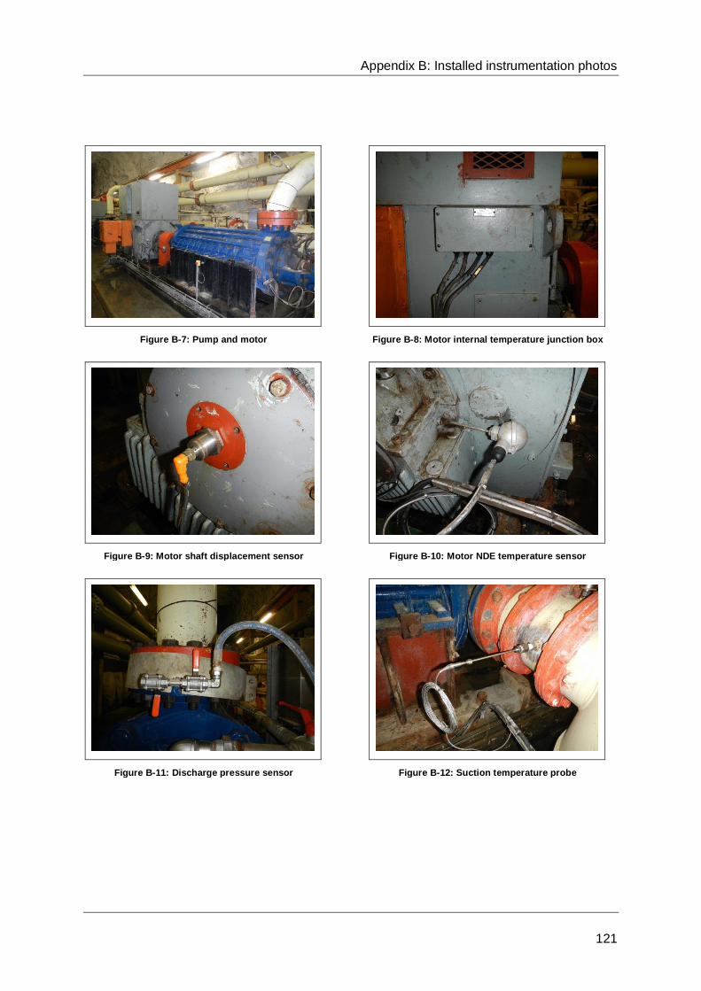
Appendix B: Installed instrumentation photos
121
Figure B-7: Pump and motor
Figure B-8: Motor internal temperature junction box
Figure B-9: Motor shaft displacement sensor
Figure B-10: Motor NDE temperature sensor
Figure B-11: Discharge pressure sensor
Figure B-12: Suction temperature probe

Appendix B: Installed instrumentation photos
122
Figure B-13: Motor DE temperature probe and
vibration sensor
Figure B-14: Discharge temperature probe
Figure B-15: Suction flow switch
Figure B-16: Discharge NRV and actuated gate valve
Figure B-17: Inlet valve position proxies
Figure B-18: Balance disc flow temperature probe
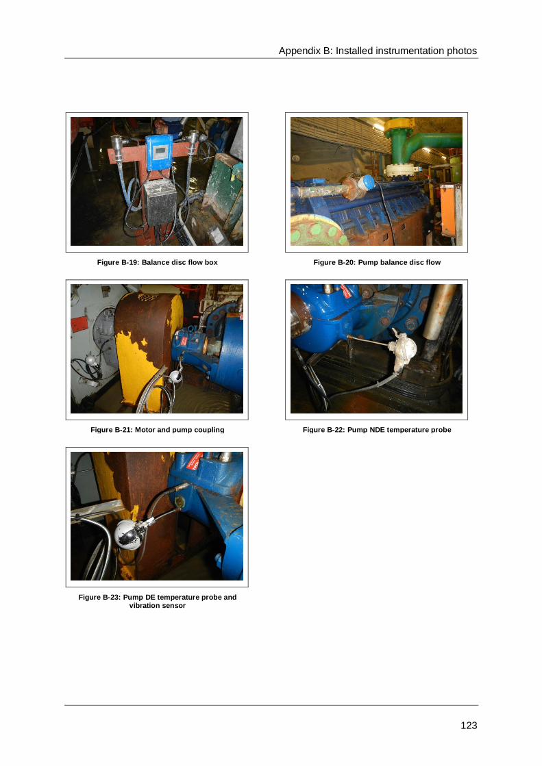
Appendix B: Installed instrumentation photos
123
Figure B-19: Balance disc flow box
Figure B-20: Pump balance disc flow
Figure B-21: Motor and pump coupling
Figure B-22: Pump NDE temperature probe
Figure B-23: Pump DE temperature probe and vibration sensor

124
Appendix C: Optimised control
C.1. Level-22
Figure C-1: Level-22 optimised control schedule
0
10
20
30
40
50
60
70
80
90
100
00:0
0
01:0
0
02:0
0
03:0
0
04:0
0
05:0
0
06:0
0
07:0
0
08:0
0
09:0
0
10:0
0
11:0
0
12:0
0
13:0
0
14:0
0
15:0
0
16:0
0
17:0
0
18:0
0
19:0
0
20:0
0
21:0
0
22:0
0
23:0
0
Up
str
eam
dam
level
[%]
Time [hh:mm]
MDL CO CR BO 1 BO2 TO1 TO2

Appendix C: Optimised control
125
Table C-1: Level-22 maximum number of pumps
Pumps
available
Level-22
Dam St1
IPCM
Dam St1
IPCM
Dam St2
Max nr
of pumps
4
>90 N/A N/A 3
<90 >90
>98 1
<98 2
<90 N/A 3
3
>90 N/A N/A 2
<90 >90
>98 0
<98 1
<90 N/A 2
2
>90 N/A N/A 2
<90 >90
>98 0
<98 1
<90 N/A 2
1
>90 N/A N/A 1
<90 >90
>98 0
<98 0
<90 N/A 1
0 N/A N/A N/A 0

Appendix C: Optimised control
126
C.2. IPC Sub optimised control schedule
Figure C-2: IPCS optimised control schedule
Table C-2: IPCS maximum number of pumps
Pumps
available
IPCS
Dam St2
Level-22
Dam St1
Level-22
Dam St2
Max nr
of pumps
4
>90 N/A N/A 3
<90 >85
>90 1
<90 2
<85 N/A 3
3
>90 N/A N/A 2
<90 >85
>90 0
<90 1
<85 N/A 2
2
>90 N/A N/A 2
<90 >85
>90 0
<90 1
<85 N/A 2
1
>90 N/A N/A 1
<90 >85
>90 0
<90 0
<85 N/A 1
0 N/A N/A N/A 0
0
10
20
30
40
50
60
70
80
90
1000
0:0
0
01:0
0
02:0
0
03:0
0
04:0
0
05:0
0
06:0
0
07:0
0
08:0
0
09:0
0
10:0
0
11:0
0
12:0
0
13:0
0
14:0
0
15:0
0
16:0
0
17:0
0
18:0
0
19:0
0
20:0
0
21:0
0
22:0
0
23:0
0
Up
str
ea
m d
am
le
ve
l [%
]
Time [hh:mm]
MDL CO CR BO 1 BO2 TO1 TO2

Appendix C: Optimised control
127
C.3. Level-46 optimised control schedule
Figure C-3: Level-46 optimised control schedule
Table C-3: Level-46 maximum number of pumps
Pumps
available
Level-46
Dam St2
IPCS
Dam St1
IPCS
Dam St2
Max nr
of pumps
4
>90 N/A N/A 3
<90 >97
>99 1
<99 2
<97 N/A 3
3
>90 N/A N/A 2
<90 >97
>99 0
<99 1
<97 N/A 2
2
>90 N/A N/A 2
<90 >97
>99 0
<99 1
<97 N/A 2
1
>90 N/A N/A 1
<90 >97
>99 0
<99 0
<97 N/A 1
0 N/A N/A N/A 0
0
10
20
30
40
50
60
70
80
90
1000
0:0
0
01:0
0
02:0
0
03:0
0
04:0
0
05:0
0
06:0
0
07:0
0
08:0
0
09:0
0
10:0
0
11:0
0
12:0
0
13:0
0
14:0
0
15:0
0
16:0
0
17:0
0
18:0
0
19:0
0
20:0
0
21:0
0
22:0
0
23:0
0
Up
str
ea
m d
am
le
ve
l [%
]
Time [hh:mm]
MDL CO CR BO 1 BO2 TO1 TO2
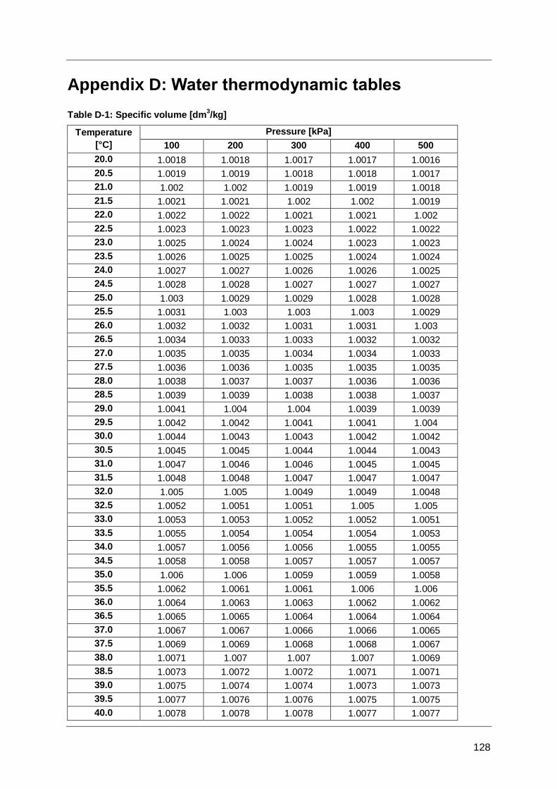
128
Appendix D: Water thermodynamic tables
Table D-1: Specific volume [dm3/kg]
Temperature
[°C]
Pressure [kPa]
100 200 300 400 500
20.0 1.0018 1.0018 1.0017 1.0017 1.0016
20.5 1.0019 1.0019 1.0018 1.0018 1.0017
21.0 1.002 1.002 1.0019 1.0019 1.0018
21.5 1.0021 1.0021 1.002 1.002 1.0019
22.0 1.0022 1.0022 1.0021 1.0021 1.002
22.5 1.0023 1.0023 1.0023 1.0022 1.0022
23.0 1.0025 1.0024 1.0024 1.0023 1.0023
23.5 1.0026 1.0025 1.0025 1.0024 1.0024
24.0 1.0027 1.0027 1.0026 1.0026 1.0025
24.5 1.0028 1.0028 1.0027 1.0027 1.0027
25.0 1.003 1.0029 1.0029 1.0028 1.0028
25.5 1.0031 1.003 1.003 1.003 1.0029
26.0 1.0032 1.0032 1.0031 1.0031 1.003
26.5 1.0034 1.0033 1.0033 1.0032 1.0032
27.0 1.0035 1.0035 1.0034 1.0034 1.0033
27.5 1.0036 1.0036 1.0035 1.0035 1.0035
28.0 1.0038 1.0037 1.0037 1.0036 1.0036
28.5 1.0039 1.0039 1.0038 1.0038 1.0037
29.0 1.0041 1.004 1.004 1.0039 1.0039
29.5 1.0042 1.0042 1.0041 1.0041 1.004
30.0 1.0044 1.0043 1.0043 1.0042 1.0042
30.5 1.0045 1.0045 1.0044 1.0044 1.0043
31.0 1.0047 1.0046 1.0046 1.0045 1.0045
31.5 1.0048 1.0048 1.0047 1.0047 1.0047
32.0 1.005 1.005 1.0049 1.0049 1.0048
32.5 1.0052 1.0051 1.0051 1.005 1.005
33.0 1.0053 1.0053 1.0052 1.0052 1.0051
33.5 1.0055 1.0054 1.0054 1.0054 1.0053
34.0 1.0057 1.0056 1.0056 1.0055 1.0055
34.5 1.0058 1.0058 1.0057 1.0057 1.0057
35.0 1.006 1.006 1.0059 1.0059 1.0058
35.5 1.0062 1.0061 1.0061 1.006 1.006
36.0 1.0064 1.0063 1.0063 1.0062 1.0062
36.5 1.0065 1.0065 1.0064 1.0064 1.0064
37.0 1.0067 1.0067 1.0066 1.0066 1.0065
37.5 1.0069 1.0069 1.0068 1.0068 1.0067
38.0 1.0071 1.007 1.007 1.007 1.0069
38.5 1.0073 1.0072 1.0072 1.0071 1.0071
39.0 1.0075 1.0074 1.0074 1.0073 1.0073
39.5 1.0077 1.0076 1.0076 1.0075 1.0075
40.0 1.0078 1.0078 1.0078 1.0077 1.0077

Appendix D: Water thermodynamic tables
129
Table D-2: Specific heat [J/kg.K-1
]
Temperature
[°C]
Pressure [kPa]
100 200 300 400 500
20.0 4184.1 4183.7 4183.4 4183.1 4182.8
20.5 4183.7 4183.4 4183.1 4182.8 4182.5
21.0 4183.4 4183.1 4182.8 4182.5 4182.2
21.5 4183.1 4182.8 4182.5 4182.2 4181.9
22.0 4182.8 4182.5 4182.2 4181.9 4181.6
22.5 4182.5 4182.2 4181.9 4181.6 4181.3
23.0 4182.2 4181.9 4181.6 4181.3 4181.1
23.5 4182 4181.7 4181.4 4181.1 4180.8
24.0 4181.8 4181.5 4181.2 4180.9 4180.6
24.5 4181.5 4181.2 4180.9 4180.7 4180.4
25.0 4181.3 4181 4180.7 4180.5 4180.2
25.5 4181.1 4180.8 4180.5 4180.3 4180
26.0 4180.9 4180.6 4180.4 4180.1 4179.8
26.5 4180.8 4180.5 4180.2 4179.9 4179.6
27.0 4180.6 4180.3 4180 4179.7 4179.5
27.5 4180.4 4180.2 4179.9 4179.6 4179.3
28.0 4180.3 4180 4179.7 4179.5 4179.2
28.5 4180.2 4179.9 4179.6 4179.3 4179.1
29.0 4180 4179.8 4179.5 4179.2 4178.9
29.5 4179.9 4179.7 4179.4 4179.1 4178.8
30.0 4179.8 4179.6 4179.3 4179 4178.7
30.5 4179.7 4179.5 4179.2 4178.9 4178.6
31.0 4179.6 4179.4 4179.1 4178.8 4178.6
31.5 4179.6 4179.3 4179 4178.8 4178.5
32.0 4179.5 4179.2 4179 4178.7 4178.4
32.5 4179.4 4179.2 4178.9 4178.6 4178.4
33.0 4179.4 4179.1 4178.9 4178.6 4178.3
33.5 4179.3 4179.1 4178.8 4178.6 4178.3
34.0 4179.3 4179.1 4178.8 4178.5 4178.3
34.5 4179.3 4179 4178.8 4178.5 4178.2
35.0 4179.3 4179 4178.7 4178.5 4178.2
35.5 4179.2 4179 4178.7 4178.5 4178.2
36.0 4179.2 4179 4178.7 4178.5 4178.2
36.5 4179.2 4179 4178.7 4178.5 4178.2
37.0 4179.2 4179 4178.7 4178.5 4178.2
37.5 4179.3 4179 4178.8 4178.5 4178.3
38.0 4179.3 4179 4178.8 4178.5 4178.3
38.5 4179.3 4179.1 4178.8 4178.6 4178.3
39.0 4179.3 4179.1 4178.8 4178.6 4178.3
39.5 4179.4 4179.1 4178.9 4178.6 4178.4
40.0 4179.4 4179.2 4178.9 4178.7 4178.4

Appendix D: Water thermodynamic tables
130
Table D-3: Joule-Thompson coefficient [K/MPa]
Temperature
[°C]
Pressure [kPa]
100 200 300 400 500
20.0 -0.22492 -0.22491 -0.22491 -0.2249 -0.2249
20.5 -0.22456 -0.22456 -0.22456 -0.22455 -0.22455
21.0 -0.22421 -0.22421 -0.2242 -0.2242 -0.2242
21.5 -0.22386 -0.22386 -0.22385 -0.22385 -0.22385
22.0 -0.22351 -0.22351 -0.22351 -0.2235 -0.2235
22.5 -0.22317 -0.22316 -0.22316 -0.22316 -0.22315
23.0 -0.22282 -0.22282 -0.22282 -0.22281 -0.22281
23.5 -0.22248 -0.22248 -0.22248 -0.22247 -0.22247
24.0 -0.22214 -0.22214 -0.22214 -0.22213 -0.22213
24.5 -0.2218 -0.2218 -0.2218 -0.2218 -0.22179
25.0 -0.22147 -0.22146 -0.22146 -0.22146 -0.22146
25.5 -0.22113 -0.22113 -0.22113 -0.22112 -0.22112
26.0 -0.2208 -0.2208 -0.22079 -0.22079 -0.22079
26.5 -0.22047 -0.22047 -0.22046 -0.22046 -0.22046
27.0 -0.22014 -0.22014 -0.22013 -0.22013 -0.22013
27.5 -0.21981 -0.21981 -0.21981 -0.2198 -0.2198
28.0 -0.21948 -0.21948 -0.21948 -0.21948 -0.21948
28.5 -0.21916 -0.21916 -0.21915 -0.21915 -0.21915
29.0 -0.21883 -0.21883 -0.21883 -0.21883 -0.21883
29.5 -0.21851 -0.21851 -0.21851 -0.21851 -0.21851
30.0 -0.21819 -0.21819 -0.21819 -0.21819 -0.21819
30.5 -0.21787 -0.21787 -0.21787 -0.21787 -0.21787
31.0 -0.21755 -0.21755 -0.21755 -0.21755 -0.21755
31.5 -0.21724 -0.21724 -0.21723 -0.21723 -0.21723
32.0 -0.21692 -0.21692 -0.21692 -0.21692 -0.21692
32.5 -0.21661 -0.21661 -0.21661 -0.21661 -0.2166
33.0 -0.2163 -0.21629 -0.21629 -0.21629 -0.21629
33.5 -0.21598 -0.21598 -0.21598 -0.21598 -0.21598
34.0 -0.21567 -0.21567 -0.21567 -0.21567 -0.21567
34.5 -0.21536 -0.21536 -0.21536 -0.21536 -0.21536
35.0 -0.21506 -0.21506 -0.21506 -0.21506 -0.21506
35.5 -0.21475 -0.21475 -0.21475 -0.21475 -0.21475
36.0 -0.21444 -0.21444 -0.21444 -0.21444 -0.21444
36.5 -0.21414 -0.21414 -0.21414 -0.21414 -0.21414
37.0 -0.21384 -0.21384 -0.21384 -0.21384 -0.21384
37.5 -0.21353 -0.21353 -0.21353 -0.21353 -0.21353
38.0 -0.21323 -0.21323 -0.21323 -0.21323 -0.21323
38.5 -0.21293 -0.21293 -0.21293 -0.21293 -0.21293
39.0 -0.21263 -0.21263 -0.21263 -0.21263 -0.21263
39.5 -0.21233 -0.21233 -0.21233 -0.21234 -0.21234
40.0 -0.21204 -0.21204 -0.21204 -0.21204 -0.21204