behavioral learning equilibria in the new keynesian model
TRANSCRIPT

Behavioral Learning Equilibria in the
New Keynesian Model ∗
Cars Hommesa,b , Kostas Mavromatisc , Tolga Ozdena , Mei Zhud,†
a CeNDEF, School of Economics, University of Amsterdam
and Tinbergen Institute, Netherlands
b Bank of Canada‡, Canada
c De Nederlandsche Bank and University of Amsterdam, The Netherlands
d Institute for Advanced Research & School of Economics, Shanghai University of Finance and Economics,
and the Key Laboratory of Mathematical Economics(SUFE), Ministry of Education, Shanghai 200433, China
January 21, 2020
Abstract
We introduce the concept of behavioral learning equilibrium (BLE) into a high
dimensional linear framework and apply it to the standard New Keynesian (NK)
model. For each endogenous variable, boundedly rational agents use a simple, but
optimal AR(1) forecasting rule with parameters consistent with the observed sample
mean and autocorrelation of past data. The main contributions of our paper are
fivefold: (1) we derive existence and stability conditions of BLE in a general linear
framework, (2) we provide a method for Bayesian likelihood estimation of BLE, (3)
we estimate the baseline NK model based on U.S. data and show that the relative
model fit is better under BLE than REE, (4) we show that multiple E-stable BLE
exist in plausible parameter regions characterized by a unique REE, (5) optimal
monetary policy under BLE is different from REE and typically more aggressive,
suggesting that an optimal policy under REE may perform poorly under BLE.
JEL classification: C11; E62; E03; D83; D84
Keywords: Bounded rationality; Behavioral learning equilibrium; Adaptive learn-
ing; behavioral New Keynesian macro-model; Monetary Policy.
∗Corresponding author: Cars Hommes.† E-mail addresses: [email protected], [email protected], [email protected]
[email protected]‡The views expressed in this paper do not represent the position of the Bank of Canada, De Neder-
landsche Bank or the Eurosystem.
1
Acknowledgements
Earlier versions of this paper have been presented at the Computation in Economics
and Finance (CEF) conference, June 20-22, 2015, Taipei, Taiwan; the Workshop Ex-
pectations in Dynamic Macroeconomic Models, August 13-15 2015, University of
Oregon, USA; the Workshop on Agent-Based and DSGE Macroeconomic Modeling:
Bridging the Gap, November 20, 2015, Surrey, UK; the CEF2017 conference, June
28-30, 2017, New York; Workshop on Adaptive Learning, May 7-8, 2018, Bilbao,
Spain; Behavioral Macroeconomics Workshop, June 15-16, 2018, Bamberg, Ger-
many; CEF2018 conference, June 19-21, 2018, Milano, Italy; the 14th Dynare Con-
ference, July 5-6, 2018, ECB, Frankurt, Germany; and the ESEM conference, Au-
gust 27-31, 2018, Koln, Germany. Stimulating discussions and comments from Klaus
Adam, Bill Branch, Jim Bullard, George Evans, Stephanie Schmitt-Grohe, Paul
Levine, Domenico Massaro, Bruce McGough, Bruce Preston, Sergey Slobodyan,
Gianluca Violante, Mike Woodford and Raf Wouters are gratefully acknowledged.
The research leading to these results has received funding from the European Com-
munity’s Seventh Framework Programme (FP7/2007-2013) under grant agreement
“Integrated Macro-Financial Modeling for Robust Policy Design ( MACFINRO-
BODS)”, grant no. 612796. Mei Zhu also acknowledges financial support from
NSFC funding Studies on equilibria of heterogeneous agents models under adaptive
learning (grant no. 11401365), NSFC (71850002), China Scholarship Council (file
no. 201506485009) and the Fundamental Research Funds for the Central Universi-
ties.
Disclosure Statement
The authors declare that they have no relevant material or financial interests that
relate to the research described in this paper. All authors have contributed equally
and approved the final article.
2

1 Introduction
Rational Expectations Equilibrium (REE) requires that economic agents’ subjective
probability distributions coincide with the objective distribution that is determined, in
part, by their subjective beliefs. There is a vast literature that studies the drawbacks of
REE. Some of these drawbacks include the fact that REE requires an unrealistic degree
of computational power and perfect information on the part of agents. As an alternative
to REE, the adaptive learning literature (see, e.g., Evans and Honkapohja (2001, 2013)
and Bullard (2006) for extensive surveys and references) replaces Rational Expectations
with beliefs that come from an econometric forecasting model with parameters updated
using observed time series. A large part of this literature involves studying under which
conditions learning will converge to the REE. Convergence of adaptive learning to an REE
occurs when the perceived law of motion (PLM) of agents is correctly specified. How-
ever, in general the PLM may be misspecified. As shown in White (1994), an economic
model or a probability model is only a more or less crude approximation to whatever
might be the true relationships among the observed data. Consequently it is necessary to
view economic and/or probability models as misspecified to some greater or lesser degree.
Whenever agents have misspecified PLMs, a reasonable learning process may settle down
on a misspecification equilibrium. In the literature, different types of misspecification
equilibria have been proposed, e.g. Restricted Perceptions Equilibrium (RPE) where the
forecasting model is underparameterized (Sargent, 1991; Evans and Honkapohja, 2001;
Adam, 2003; Branch and Evans, 2010) and Stochastic Consistent Expectations Equilib-
rium (SCEE) (Hommes and Sorger, 1998; Hommes et al., 2013), where agents learn the
optimal parameters of a simple, parsimonious AR(1) rule.1
A SCEE is a very natural misspecification equilibrium, where agents in the economy
do not know the actual law of motion or even recognize all relevant explanatory variables,
but rather prefer a parsimonious forecasting model. The economy is too complex to fully
understand and therefore, as a first-order approximation, agents forecast the state of the
economy by simple autoregressive models (e.g. Fuster et al., 2010). In the simplest model
applying this idea, agents run a univariate AR(1) regression to generate out-of-sample
forecasts of the state of the economy. Hommes and Zhu (2014) provide the first-order
SCEE with an intuitive behavioral interpretation and refer to them as Behavioral Learn-
ing Equilibria (BLE). Although it is possible for some agents to use more sophisticated
models, one may argue that these practices are neither straightforward nor widespread.
A simple, parsimonious BLE seems a more plausible outcome of the coordination process
of individual expectations in large complex socio-economic systems (Grandmont, 1998).
1Branch (2006) provides a stimulating survey discussing the connection between these types of mis-specification equilibria.
3

Hommes and Zhu (2014) formalize the concept of BLE in the simplest class of models
one can think of: a one-dimensional linear stochastic model driven by an exogenous linear
stochastic AR(1) process. Agents do not recognize, however, that the economy is driven
by an exogenous process, but simply forecast the state of the economy using a univariate
AR(1) rule by using past observations. The parameters of the AR(1) forecasting rule
are not free, but fixed (and learned over time) according to the observed sample average
and first-order sample autocorrelation. Within this setup, Hommes and Zhu (2014) fully
characterize the existence and multiplicity of BLE and provide stability conditions under
a simple adaptive learning scheme –Sample Autocorrelation Learning (SAC-learning).
Although this class of models is simple, it contains two important standard applications:
an asset pricing model driven by autocorrelated dividends and the New Keynesian Phillips
curve with inflation driven by autocorrelated output gap (or marginal costs). As shown
in Fuhrer (2009), however, the skeleton model of the New Keynesian Phillips curve with
AR(1) driving variable leaves implicit the determination of real output and the role of
monetary policy in influencing output and inflation.
In this paper we extend the BLE concept to a general n-dimensional linear stochastic
framework and provide a method to estimate these models under BLE. As an applica-
tion we study the standard 3-equation dynamic stochastic general equilibrium (DSGE)
model-the New Keynesian (NK) model-, its empirical fit and the role of monetary policy
under BLE. Agents’ perceived law of motion (PLM) is a simple univariate AR(1) process
for each variable to be forecasted. Two consistency requirements are imposed upon BLE
to pin down the parameters of the forecasting model: for each endogenous variable, ob-
served sample averages and first-order sample autocorrelations match the corresponding
parameters of the forecasting rule. Agents thus learn the optimal AR(1) forecasting rule
for each endogenous variable in the economy.
The main contributions of our paper are fourfold: (1) we derive existence and stability
conditions of BLE in a general linear framework, (2) we provide a simple and general
method for Bayesian likelihood estimation of BLE, (3) we estimate the baseline NK model
based on U.S. data and show that the relative model fit is better under BLE than REE,
(4) we show that multiple E-stable BLE exist in plausible parameter regions associated
by a unique REE, (5) optimal monetary policy under BLE is different from REE and
typically more aggressive, which suggests that an optimal policy under REE may perform
poorly under BLE. This result is in line with previous studies in the adaptive learning
literature, see e.g. Orphanides & Williams (2003). The main novelty in our framework is
to show this as a misspecification equilibrium outcome, whereas previous studies typically
focus on learning dynamics around a REE.
Many models of learning lead to excess volatility, where the volatility under learning is
typically higher than under REE. Our BLE model exhibits another novel feature, persis-
4

tence amplification: the persistence of inflation and output gap under BLE is significantly
higher than under REE. In fact, even when autocorrelations of the exogenous shocks
to fundamentals are small, inflation and output gap along BLE are typically near unit
root processes. As a consequence, when we estimate the NK model under BLE2, we find
important differences in parameter estimates compared with the REE. Further, optimal
monetary policy under BLE is finite for a wide range of calibrations, and the transmission
channel of monetary policy is stronger under BLE than REE at the estimated parameters.
Related literature
The issue of persistence has been of great interest to macroeconomists and policy-
makers. A number of models with frictions have been proposed to replicate persistence,
such as habit formation in consumption, indexation to lagged inflation in price-setting,
rule-of-thumb behavior, or various adjustment costs (Phelps, 1968; Taylor, 1980; Fuhrer
and Moore, 1992, 1995; Christiano et al., 2005; Smets and Wouters, 2003, 2005; Boivin
and Giannoni, 2006; Giannoni and Woodford, 2003). These models essentially improve
the empirical fit by adding lags to the model equations. Estimating these rich models
with frictions under the assumption of RE, one typically finds that substantial degrees
of persistence are supported by the data. Therefore these additional sources of persis-
tence appear necessary to match the inertia of macroeconomic variables. Estimation of
these models typically also involve highly persistent structural shocks. Our BLE model
is applied to a New Keynesian framework without habit formation or indexation, but
nevertheless exhibits strong persistence. Learning causes persistence amplification: small
autocorrelations of exogenous shocks are strongly amplified as agents learn to coordinate
on a simple AR(1) forecasting rule with near unit root parameters consistent with ob-
served sample average and sample autocorrelations. The high persistence of inflation and
output thus arises from a self-fulfilling mistake (Grandmont, 1998).
Our BLE concept fits with the literature employing adaptive learning to analyze the
evolution of U.S. inflation and monetary policy. Adaptive learning can help in under-
standing some particular historical episodes, such as high inflation in the 1980s, which
are often harder to explain under RE. For example, Orphanides and Williams (2003) con-
sider a form of imperfect knowledge in which economic agents rely on adaptive learning
to form expectations. This form of learning represents a relatively modest deviation from
RE that nests it as a limiting case. They find that policies that would be efficient under
RE can perform poorly when knowledge is imperfect. Milani (2005, 2007) also assumes
2The empirical results presented in this paper also hold in more realistic setups. In particular, anestimated hybrid version of the New Keynesian model with lagged inflation and output can be found inour Online Appendix. We also estimate Smets-Wouters (2007) model under BLE in our follow-up paperHommes et. al. (2019).
5
that agents form expectations through adaptive learning using correctly specified eco-
nomic models and updating the parameters through constant-gain learning (CGL) based
on historical data. He shows empirically that when learning replaces RE, the estimated
degrees of habit formation and indexation drop closer to zero, suggesting that persistence
arises in the model economy mainly from expectations and learning. Eusepi and Preston
(2011) study expectations-driven business cycles based on learning, and find that learn-
ing dynamics generate forecast errors similar to the Survey of Professional Forecasters.
Estrella and Fuhrer (2002) study the shortcomings of REE models with a focus on iner-
tia and shock propagation structure. Fuhrer (2009) provides a good survey on inflation
persistence. He examines a number of empirical measures of reduced form persistence
including the first-order autocorrelation and the autocorrelation function of the inflation
series. He also investigates the sources of persistence, including learning of agents in a
RE setting.
Numerous empirical studies show that overly parsimonious models with little parame-
ter uncertainty can provide better forecasts than models consistent with the actual data-
generating complex process (e.g. Nelson, 1972; Stock and Watson, 2007; Clark and West,
2007; Enders, 2010). In a similar vein (but without analytical results) Slobodyan and
Wouters (2012) study a New Keynesian DSGE model with agents using a constant gain
AR(2) forecasting rule. Chung and Xiao (2014) and Xiao and Xu (2014) study learning
and predictions with an AR(1) or VAR(1) model in a two dimensional New Keynesian
model with limited information and show, based on simulations, that the simple AR(1)
model is more likely to prevail in reality when they make predictions. Laboratory ex-
periments in the NK framework also show that simple forecasting rules such as AR(1)
describe individual forecasting behavior surprisingly well (Assenza et al., 2014; Pfajfar
and Zakelj, 2016).
Our behavioral learning equilibrium concept is closely related to the Exuberance Equi-
libria (EE) in Bullard et al. (2008), where agents’ perceived law of motion is misspecified.
However, because of difficulty of computation, in Bullard et al. (2008) there are only
numerical results on the exuberance equilibria, while here we analytically show the exis-
tence and stability of BLE in a general linear framework with an application to the NK
model, as well as empirically validate BLE based on U.S. data. Another related mis-
specification equilibrium is Limited Information Learning Equilibrium (LILE) defined in
Chung and Xiao (2014), which is defined by the least-squares projection of variables on
the past information of the actual law of motion equal to that in the perceived law of
motion. Different from the LILE, our general Behavioral Learning Equilibrium is defined
by the conditions that sample means and first-order autocorrelations of each variable of
the actual law of motion are consistent with those corresponding to the perceived law of
motion. We further study the effects of monetary policy under the more plausible BLE.
6

The concept of natural expectations in Fuster et al. (2010) and Fuster et al. (2011, 2012)
is another related misspecification concept, where agents use simple, misspecified models,
e.g., linear autoregressive models. Natural expectations, however, do not pin down the
parameters of the forecasting model through consistency requirements as for a restricted
perceptions equilibrium nor do they allow the agents to learn an optimal misspecified
model through empirical observations. Cho and Kasa (2015) study model validation in
an environment where agents are aware of misspecification and try to detect it through
adaptive learning. Similarly, Cho and Kasa (2017) study learning in a framework where
agents form expectations using a Bayesian averaging based on multiple models. In our
BLE misspecification is self-fulfilling and it is the outcome of a learning process. Another
related work is Adam and Marcet (2011), who introduce a more sophisticated notion of
bounded rationality called internal rationality, and show that even for a small deviation
from REE beliefs, with a small prior around the correct REE belief, the outcome of the
learning model can be quite different.
The paper is organized as follows. Section 2 introduces the main concepts of BLE in
a general n-dimensional setup, the theoretical results on existence and stability of BLE in
a linear framework and the empirical estimation methodology. Section 3 applies BLE to
the 3-equation New Keynesian model and presents the existence, stability and estimation
results. Section 4 studies optimal monetary policy and how policy can mitigate persistence
and volatility amplification under BLE. Section 5 concludes.
2 BLE in a Multivariate Framework
Hommes and Zhu (2014) introduced BLE in the simplest setting, a one-dimensional
linear stochastic model driven by an exogenous linear stochastic AR(1) process. In this
paper we generalize BLE to n-dimensional (linear) stochastic models driven by exogenous
linear stochastic AR(1) processes of multiple shocks. To ease the exposition we initially
follow the presentation in Hommes and Zhu (2014), but generalize their 1-dimensional
model to an n-dimensional framework. In addition, most macroeconomic models include
lagged state variables through features such as interest rate smoothing, habit formation in
consumption or indexation in prices and wages. Therefore, we further extend the model
with lagged state variables.
Let the law of motion of an economic system be given by the stochastic difference
equation
xxxt = FFF (xxxet+1, xxxt−1, uuut, vvvt), (2.1)
where xxxt is an n×1 vector of endogenous variables denoted by [x1t, x2t, · · · , xnt]′ and xxxet+1
7

is the expected value of xxx at date t + 1. This notation highlights that expectations may
not be rational. Here FFF is a continuous n-dimensional vector function, uuut is a vector of
exogenous stationary variables and vvvt is a vector of white noise disturbances.
Agents are boundedly rational and do not know the exact form of the actual law of
motion (2.1). They only use a simple, parsimonious forecasting model where agents’ per-
ceived law of motion (PLM) is a simple univariate AR(1) process for each variable to
be forecasted. As shown in Enders (2010, p.84-85), coefficient uncertainty increases as
the model becomes more complex, and hence it could be that an estimated AR(1) model
forecasts a real ARMA(2,1) process better than an estimated ARMA(2,1) model. Nu-
merous empirical studies also show that overly parsimonious models with little parameter
uncertainty can provide better forecasts than models consistent with the more complex
actual data-generating process (e.g. Nelson, 1972; Stock and Watson, 2007; Clark and
West, 2007). Thus agents’ perceived law of motion (PLM) is assumed to be the simplest
VAR model with minimum parameters, i.e. a restricted VAR(1) process
xxxt = ααα + βββ(xxxt−1 −ααα) + δδδt, (2.2)
where ααα is a vector denoted by [α1, α2, · · · , αn]′, βββ is a diagonal matrix3 denoted byβ1 0 · · · 0
0 β2 · · · 0
· · ·0 0 · · · βn
with βi ∈ (−1, 1) and δδδt is a white noise process; ααα is the un-
conditional mean of xxxt and βi is the first-order autocorrelation coefficient of variable xi.
Given the perceived law of motion (2.2), the 2-period ahead forecasting rule for xxxt+1 that
minimizes the mean-squared forecasting error is
xxxet+1 = α + β2(xt−1 − α)α + β2(xt−1 − α)α + β2(xt−1 − α). (2.3)
Combining the expectations (2.3) and the law of motion of the economy (2.1), we obtain
the implied actual law of motion (ALM)
xxxt = FFF (ααα + βββ2(xxxt−1 −ααα), xxxt−1, uuut, vvvt). (2.4)
In the case that the ALM (2.4) is stationary, let the variance-covariance matrix ΓΓΓ(0) :=
E[(xxxt−xxx)(xxxt−xxx)′] and the first order autocovariance matrix ΓΓΓ(1) := E[(xxxt−xxx)(xxxt+1−xxx)′],
3Chung and Xiao (2014) also argue using simulations that the simple AR(1) model is more likelyto prevail in reality because of limited information restrictions when they model predictions in a twodimensional New Keynesian model. In addition, as far as prediction is concerned, based on our numerousempirical analyses, the short-term forecasts based on an AR(1) model are better than more general VARmodels in most cases, because in more general VAR models too many parameters need to be estimatedand hence coefficient uncertainty increases.
8
where xxx is the mean of xxxt. Let ΩΩΩ be the diagonal matrix in which the ith diagonal
element is the variance of the ith process, that is ΩΩΩ = diag[γ11(0), γ22(0), · · · , γnn(0)],
where γii(0) is the ith diagonal entry of ΓΓΓ(0). Let LLL be the diagonal matrix in which
the ith diagonal element is the first-order autocovariance of the ith process, that is LLL =
diag[γ11(1), γ22(1), · · · , γnn(1)], where γii(1) is the ith diagonal entry of ΓΓΓ(1). LetGGG denote
the diagonal matrix in which the ith diagonal element is the first-order autocorrelation
coefficient of the ith process xi,t. Hence
GGG = LLLΩΩΩ−1. (2.5)
Behavioral Learning Equilibrium (BLE)
Extending Hommes and Zhu (2014), the concept of BLE is generalized as follows.
Definition 2.1 A vector (µ,ααα,βββ), where µ is a probability measure, ααα is a vector and βββ
is a diagonal matrix with βi ∈ (−1, 1) (i = 1, 2, · · · , n), is called a Behavioral Learning
Equilibrium (BLE) if the following three conditions are satisfied:
S1 The probability measure µ is a nondegenerate invariant measure for the stochastic
difference equation (2.4);
S2 The stationary stochastic process defined by (2.4) with the invariant measure µ has
unconditional mean ααα, that is, the unconditional mean of xi is αi, (i = 1, 2, · · · , n);
S3 Each element xi for the stationary stochastic process of xxx defined by (2.4) with the
invariant measure µ has unconditional first-order autocorrelation coefficient βi, (i =
1, 2, · · · , n), that is, GGG = βββ.
In other words, a BLE is characterized by two natural observable consistency require-
ments: the unconditional means and the unconditional first-order autocorrelation coef-
ficients generated by the actual (unknown) stochastic process (2.4) coincide with the
corresponding statistics for the perceived linear VAR(1) process (2.2), as given by the pa-
rameters ααα and βββ. This means that in a BLE agents correctly perceive the two simplest
and most important statistics: the mean and first-order autocorrelation (i.e., persistence)
of each relevant variable of the economy, without fully understanding its structure and
recognizing all explanatory variables and cross-correlations. A BLE is parameter free,
as along a BLE the two parameters of each linear forecasting rule are pinned down by
simple and observable statistics. Hence, agents do not fully understand the linear struc-
ture of the stochastic economy, i.e. they do not observe the shocks and do not take the
cross-correlations of state variables into account, but rather use a parsimonious univariate
AR(1) forecasting rule for each state variable. A simple BLE may be a plausible outcome
9

of the coordination process of expectations of a large population. Laboratory experiments
within the New Keynesian framework also provide empirical evidence of the use of sim-
ple univariate AR(1) forecasting rules to forecast inflation and output gap (Adam, 2007;
Pfajfar and Zakelj, 2016; Assenza et al., 2014).
Furthermore, we note that along a BLE the orthogonality condition
E[xi,t − αi − βi(xi,t−1 − αi)] = 0,
E[xi,t − αi − βi(xi,t−1 − αi)]xi,t−1 = E[xi,t − αi − βi(xi,t−1 − αi)](xi,t−1 − αi) = 0
is satisfied. That is, the forecast αi + βi(xi,t−1 − αi) is the linear projection of xi,t on
the vector (1, xi,t−1)′. For each variable, agents cannot detect the correlation between
the forecasting error xi,t − αi − βi(xi,t−1 − αi) and the vector (1, xi,t−1)′ in the forecast
model. The linear projection produces the smallest mean squared error among the class
of linear forecasting rules (e.g., Hamilton (1994)). Therefore, for each variable agents
use the optimal forecast within their class of univariate AR(1) forecasting rules (Branch,
2006).
Sample autocorrelation learning
In the above definition of BLE, agents’ beliefs are described by the linear forecasting
rule (2.3) with fixed parameters ααα and βββ. However, the parameters ααα and βββ are usually
unknown to agents. In the adaptive learning literature, it is common to assume that agents
behave like econometricians using time series observations to estimate the parameters as
new observations become available. Following Hommes and Sorger (1998), we assume
that agents use sample autocorrelation learning (SAC-learning) to learn the parameters
αi and βi, i = 1, 2, · · · , n. That is, for any finite set of observations xi,0, xi,1, · · · , xi,t,the sample average is given by
αi,t =1
t+ 1
t∑k=0
xi,k, (2.6)
and the first-order sample autocorrelation coefficient is given by
βi,t =
∑t−1k=0(xi,k − αi,t)(xi,k+1 − αi,t)∑t
k=0(xi,k − αi,t)2. (2.7)
Hence αi,t and βi,t are updated over time as new information arrives. It is easy to check
that, independently of the choice of the initial values (xi,0, αi,0, βi,0), it always holds that
βi,1 = −12, and that the first-order sample autocorrelation βi,t ∈ [−1, 1] for all t ≥ 1.
10

As shown in Hommes and Zhu (2014), define
Ri,t =1
t+ 1
t∑k=0
(xi,k − αi,t)2.
Then SAC-learning is equivalent to the following recursive dynamical system4:
αi,t = αi,t−1 +1
t+ 1(xi,t − αi,t−1),
βi,t = βi,t−1 +1
t+ 1R−1i,t
[(xi,t − αi,t−1)
(xi,t−1 +
xi,0t+ 1
− t2 + 3t+ 1
(t+ 1)2αi,t−1 −
1
(t+ 1)2xi,t)
− t
t+ 1βi,t−1(xi,t − αi,t−1)2
],
Ri,t = Ri,t−1 +1
t+ 1
[ t
t+ 1(xi,t − αi,t−1)2 −Ri,t−1
].
(2.8)
The actual law of motion under SAC-learning is therefore given by
xxxt = FFF (αααt−1 + βββ2t−1(xxxt−1 −αααt−1), xxxt−1, uuut, vvvt), (2.9)
with αi,t, βi,t as in (2.8).
In Hommes and Zhu (2014), F is a one-dimensional linear function. In this paper FFF
may be an n-dimensional linear vector function and includes the lagged term xxxt−1.
2.1 Main results in a multivariate linear framework
Assume that a reduced form model is an n-dimensional linear stochastic process xxxt,
driven by an exogenous VAR(1) process uuut. More precisely, the actual law of motion of
the economy is given by
xxxt = FFF (xxxet+1, uuut, vvvt) = bbb0 + bbb1xxxet+1 + bbb2xxxt−1 + bbb3uuut + bbb4vvvt, (2.10)
uuut = aaa+ ρρρuuut−1 + εεεt, (2.11)
where xxxt is an n×1 vector of endogenous variables, bbb0 and aaa are vectors of constants, bbb1, bbb2
and bbb4 are n× n matrices of coefficients, bbb3 is an n×m matrix, ρρρ is an m×m matrix, uuut
is an m× 1 vector of exogenous variables which is assumed to follow a stationary VAR(1)
4The system in (2.8) is a decreasing gain algorithm, where all observations receive equal weight andtherefore the weight on the latest observation decreases as the sample size grows. There is also a constantgain correspondence of SAC-learning, where past observations are discounted at a geometric rate. Thiscan be obtained by replacing the weights 1
t+1 by some positive constant κ, see the online appendix toHommes & Zhu (2014) for further details.
11

as in (2.11), and vvvt is an n × 1 vector of i.i.d. stochastic disturbance terms with mean
zero and finite absolute moments, with variance-covariance matrix ΣvvvΣvvvΣvvv. Hence all of the
eigenvalues of ρρρ are assumed to be inside the unit circle. In addition, εεεt is assumed to be
an m× 1 vector of i.i.d. stochastic disturbance terms with mean zero and finite absolute
moments, with variance-covariance matrix ΣεΣεΣε and is independent of vvvt.
Rational expectations equilibrium
Assume that agents are rational. The perceived law of motion (PLM) corresponding
to the minimum state variable REE of the model is:
xxx∗t = ccc0 + ccc1xxx∗t−1 + ccc2uuut + ccc3vvvt. (2.12)
Assuming that shocks uuut are observable when forecasting xxxt+1, the one-step ahead forecast
is:
Etxxx∗t+1 = ccc0 + ccc2aaa+ ccc1xxx
∗t + ccc2ρρρuuut, (2.13)
and the corresponding actual law of motion is:
xxx∗t = bbb0 + bbb1(ccc0 + ccc2aaa+ ccc1xxx∗t + ccc2ρρρuuut) + bbb2xxxt−1 + bbb3uuut + bbb4vvvt. (2.14)
The rational expectations equilibrium (REE) is the fixed point of
ccc0 − bbb1ccc1ccc0 − bbb1ccc0 = bbb0 + bbb1ccc2aaa, (2.15)
ccc1 − bbb1ccc21 = bbb2, (2.16)
ccc2 − bbb1ccc1ccc2 − bbb1ccc2ρρρ = bbb3, (2.17)
ccc3 − bbb1ccc1ccc3 = bbb4. (2.18)
A straightforward computation (see Appendix A) shows that the mean of the REE xxx∗
satisfies
xxx∗ = (III − bbb1 − bbb2)−1[bbb0 + bbb3(I − ρρρ)−1a(I − ρρρ)−1a(I − ρρρ)−1a], (2.19)
where III denotes a comfortable identity matrix throughout the paper. In the special case
with ρρρ = ρIII 5 and bbb2 = 000, the rational expectations equilibrium xxx∗t satisfies
xxx∗t = (III − bbb1)−1bbb0 + (III − bbb1)−1bbb1(III − ρbbb1)−1bbb3aaa+ (III − ρbbb1)−1bbb3uuut + bbb4vvvt. (2.20)
5Note that ρρρ is a matrix while ρ is a scalar number throughout the paper.
12

Thus its unconditional mean is:
xxx∗ = E(xxx∗t ) = (1− ρ)−1(III − bbb1)−1[bbb0(1− ρ) + bbb3aaa]. (2.21)
Its variance-covariance matrix is:
ΣΣΣxxx∗ = E[(xxx∗t − xxx∗)(xxx∗t − xxx∗)′] = (1− ρ2)−1(III − ρbbb1)−1bbb3ΣεεεΣεεεΣεεε[(III − ρbbb1)−1bbb3]
′+ bbb4ΣvΣvΣvbbb
′4.(2.22)
Furthermore, the first-order autocovariance is
ΣΣΣxxx∗xxx∗−1= E[(xxx∗t − xxx∗)(xxx∗t−1 − xxx∗)
′] = ρ(1− ρ2)−1(III − ρbbb1)−1bbb3ΣεεεΣεεεΣεεε[(III − ρbbb1)−1bbb3]
′. (2.23)
The first-order autocorrelation of the i-th-element x∗i of xxx∗ is the i-th diagonal element of
matrix ΣΣΣxxx∗xxx∗−1divided by the corresponding i-th diagonal element of matrix ΣΣΣxxx∗ . Further-
more, if ΣvvvΣvvvΣvvv = 000, then the first-order autocorrelation of the i-th element ui of uuu is equal to
ρ. In this case the persistence of the i-th variable x∗i in the REE coincides exactly with
the persistence of the exogenous driving force ui,t. That is, in this case the persistence in
the REE only inherits the persistence of the exogenous driving force.
Existence of BLE
Now assume that agents are boundedly rational and do not believe or recognize that
the economy is driven by an exogenous VAR(1) process uuut, but use a simple univariate
linear rule to forecast the state xxxt of the economy. Given that agents’ perceived law of
motion is a restricted VAR(1) process as in (2.2), the actual law of motion becomes
xxxt = bbb0 + bbb1[ααα + βββ2(xxxt−1 −ααα)] + bbb2xxxt−1 + bbb3uuut + bbb4vvvt, (2.24)
with uuut given in (2.11). If all eigenvalues of bbb1βββ2 + bbb2, for each βi ∈ [−1, 1], 1 ≤ i ≤ n, lie
inside the unit circle, then the system (2.24) of xxxt is stationary and hence its mean xxx and
first-order autocorrelation GGG exist.
The mean of xxxt in (2.24) is computed as
xxx = (III − bbb1βββ2 − bbb2)−1[bbb0 + bbb1ααα− bbb1βββ
2ααα + bbb3(III − ρρρ)−1aaa]. (2.25)
Imposing the first consistency requirement of a BLE on the mean, i.e. xxx = ααα, and solving
for ααα yields
ααα∗ = (III − bbb1 − bbb2)−1[bbb0 + bbb3(III − ρρρ)−1aaa]. (2.26)
Comparing with (2.19), we conclude that in a BLE the unconditional mean ααα∗ coincides
with the REE mean. That is to say, in a BLE the state of the economy xxxt fluctuates on
13

average around its RE fundamental value xxx∗.
Consider the second consistency requirement of a BLE on the first-order autocorrela-
tion coefficient matrix βββ of the PLM. The second consistency requirement yields
GGG(βββ) = βββ, (2.27)
whereGGG as in (2.5) and βββ are diagonal matrices. For convenience let Gi denote the i-th
diagonal element of the matrixGGG in (2.5). Under the assumption that all of the eigenvalues
of bbb1βββ2 + bbb2 for each βi ∈ [−1, 1](i = 1, 2, · · · , n) lie inside the unit circle, from the theory
of stationary linear time series, Gi(β1, β2, · · · , βn) ∈ [−1, 1] and is a continuous function
with respect to (β1, β2, · · · , βn) and other model parameters, see Appendix B6. Based
on Brouwer’s fixed-point theorem for (G1, G2, · · · , Gn), there exists βββ∗ = (β∗1 , β∗2 , · · · , β∗n)
with each β∗i ∈ [−1, 1], such that GGG(β∗β∗β∗) = β∗β∗β∗. We conclude:
Proposition 1 If all eigenvalues of ρρρ and bbb1βββ2 + bbb2, for each βi ∈ [−1, 1], are inside
the unit circle7, there exists at least one behavioral learning equilibrium (ααα∗,βββ∗) for the
economic system (2.24) with ααα∗ = (III − bbb1 − bbb2)−1[bbb0 + bbb3(III − ρρρ)−1aaa] = xxx∗.
Stability under SAC-learning
In this subsection we study the stability of BLE under SAC-learning. The ALM of
the economy under SAC-learning is given byxxxt = bbb0 + bbb1[αααt−1 + βββ2
t−1(xxxt−1 −αααt−1)] + bbb2xxxt−1 + bbb3uuut + bbb4vvvt,
uuut = aaa+ ρρρuuut−1 + εεεt.(2.28)
with αααt, βββt updated based on realized sample average and sample autocorrelation as in
(2.8). Appendix C shows that the E-stability principle applies and that stability under
SAC-learning is determined by the associated ordinary differential equation (ODE)8
dααα
dτ= xxx(ααα,βββ)−ααα = (III − bbb1βββ
2 − bbb2)−1[bbb0 + bbb1ααα− bbb1βββ2ααα + bbb3(III − ρρρ)−1aaa]−ααα,
dβββ
dτ= GGG(βββ)− βββ,
(2.29)
6For example, refer to the expression (3.9) in Hommes and Zhu (2014) for the special 1-dimensionalcase n = 1 and bbb2 = 000. In Section 3 we consider the New Keynesian model with two forward-lookingvariables and compute the (complicated) expressions of G1(β1, β2) and G2(β1, β2) explicitly.
7The Schur-Cohn criterion theorem provides necessary and sufficient conditions for all eigenvalues tolie inside the unit circle, see Elaydi (1999). For specific models, one may find sufficient conditions that areindependent of βββ to guarantee that all eigenvalues of bbb1βββ
2 + bbb2, for each βi ∈ [−1, 1], are inside the unitcircle. For example, in the case of the NK model, the Taylor principle is a sufficient condition to ensurethat all eigenvalues of bbb1βββ
2 + bbb2 lie inside the unit circle for all βi ∈ [−1, 1]; see Section 3.2, Corollary 2and Appendix E.
8See Evans and Honkapohja (2001) for a discussion and mathematical treatment of E-stability.
14
where xxx(ααα,βββ) is the mean given by (2.25) and GGG(βββ) is the diagonal first-order autocorre-
lation matrix. A BLE (ααα∗,βββ∗) corresponds to a fixed point of the ODE (2.29). Moreover,
a BLE (ααα∗,βββ∗) is locally stable under SAC-learning if it is a stable fixed point of the ODE
(2.29). Therefore, we have the following property of SAC-learning stability:
Proposition 2 A BLE (ααα∗,βββ∗) is locally stable (E-stable) under SAC-learning if
(i) all eigenvalues of (III − bbb1βββ∗2 − bbb2)−1(bbb1 + bbb2 − III) have negative real parts9, and
(ii) all eigenvalues of DDDGGGβββ(βββ∗) have real parts less than 1, where DDDGGGβββ is the Jacobian
matrix with the (i, j)-th entry ∂Gi∂βj
.
Proof. See Appendix C.
Recall from Subsection 2.1 that Gi(β1, β2, · · · , βn) ∈ (−1, 1) so that at least one BLE
exists. The proposition above implies that the BLE may be E-stable under SAC-learning.
2.2 Estimation of BLE
As our application to the NK model will illustrate in the next section, finding an
analytical expression for a BLE is usually not possible. Therefore we provide a general
numerical iteration method to estimate a BLE of the linear system (2.10) and (2.11).
The main challenge here is the joint estimation of the structural parameters and the BLE
belief parameters βββ∗ that satisfy a highly non-linear consistency (fixed point) constraint
βββ∗ = G(βββ∗). The estimation method proceeds in two steps: we first use the notion of
iterative E-stability to find an approximate BLE for a given set of structural parameters,
as described in Algorithm I below. An advantage of this method is that when it converges,
the BLE must be stable under adaptive learning. We next propose an iterative estimation
procedure for the structural and the belief parameters as summarized in Algorithm II
below, which is closely linked to the notion of iterative E-stability and which is a recursion
of Bayesian estimations of linear models. We first re-write the system by augmenting xxxt
with uuut to obtain[III −b−b−b3
000 III
][xxxt
uuut
]=
[bbb0
aaa
]+
[bbb2 000
000 ρρρ
][xxxt−1
uuut−1
]+
[bbb1 000
000 000
][xxxet+1
uuuet+1
]+
[bbb4 000
000 III
][vvvt
εεεt
]. (2.30)
Define10 [xxxt
uuut
]= St,
[vvvt
εεεt
]= ηt,
[III −b−b−b3
000 III
]= γ, γ−1
[bbb0
aaa
]= γ, γ−1
[bbb2 000
000 ρρρ
]= γ1,
9The Routh-Hurwitz criterion theorem provides sufficient and necessary conditions for all the n eigen-values having negative real parts, see Brock and Malliaris (1989).
10We assume the invertibility conditions of the corresponding matrices are satisfied throughout thepaper.
15

γ−1
[bbb1 000
000 000
]= γ2, γ
−1
[bbb4 000
000 III
]= γ3.
We can then re-write the law of motion as
St = γ + γ1St−1 + γ2Set+1 + γ3ηt. (2.31)
The agent’s PLM, the corresponding one-step ahead expectations and the implied
ALM are given as11
St = ααα + βββ(St−1 −ααα) + δtδtδt,
Set+1 = ααα + βββ2(St−1 −ααα),
St = (γ + γ2(ααα− βββ2ααα)) + γ1St−1 + γ2βββ2St−1 + γ3ηt.
(2.32)
Our main goal in this section is to estimate log-linearized DSGE models, where the mean
α∗α∗α∗ is available based on (2.26). Without loss of generality, we focus on the case where
α∗α∗α∗ = 0. Denoting by ΓΓΓ(0) and ΓΓΓ(1) the variance-covariance and first-order covariance
matrices as before, one can show that12
V ec(ΓΓΓ(0)) = [I −M(β∗β∗β∗)⊗M(β∗β∗β∗)]−1(γ3 ⊗ γ3)V ec(ΣηΣηΣη),
V ec(ΓΓΓ(1)) = [I ⊗M(β∗β∗β∗)]V ec(ΓΓΓ(0)),(2.33)
where M(βββ∗) = γ1 + γ2β∗β∗β∗2, and ΣηΣηΣη is the variance-covariance matrix of i.i.d disturbances
ηt. This implies that βj∗ =
V ec(ΓΓΓ(1))N(j−1)+j
V ec(ΓΓΓ(0))N(j−1)+j= Gj(βββ
∗, θ), 1 ≤ j ≤ N , where θ represents
the set of structural parameters in γ1, γ2 and γ3. Then every BLE satisfiesSt = γ1St−1 + γ2β∗β∗β∗2St−1 + γ3ηt,
β∗j =V ec(V ec(ΓΓΓ(1))N(j−1)+j
V ec(ΓΓΓ(0))N(j−1)+j= Gj(βββ
∗, θ), 1 ≤ j ≤ N.(2.34)
The E-stability conditions of Proposition 2 are easily simplified to the case with zero mean.
Accordingly, a BLE (000, βββ∗) is locally stable if all eigenvalues of (I−γ1−γ2β∗β∗β∗2)(γ1 +γ2−I)
have negative real parts and all eigenvalues of DGβββ(βββ∗) have real parts less than one. Note
that the first condition governs the stability of mean coefficients, while the second condi-
tion relates to stability of first-order autocorrelation coefficients independent of α∗α∗α∗.
11Without loss of generality, we assume the first N variables in St are the forward-looking variablesand we introduce zeros for the remaining state variables and exogenous shocks.
12See Appendix B.
16

Iterative E-stability and Estimation of BLE
The first-order autocorrelation coefficients βββ∗ in (2.34) are functions in terms of the
structural parameters θ, which satisfy the nonlinear equilibrium conditions G(βββ∗, θ) = βββ∗
and cannot be computed analytically. In order to find a BLE for a given θ, we use a
simple fixed-point iteration, which is formalized below in Algorithm I.
Algorithm I: Approximation of a BLE using Iterative E-stability
Denote by θ the set of structural parameters, and by G(β(k)β(k)β(k), θ) the first-order autocorre-lation function for a given θ.
• Step (0): Initialize the vector of learning parameters at β(0)β(0)β(0).
• Step (I): At each iteration k, using the first-order autocorrelation functions, updatethe vector of learning parameters as
β(k)β(k)β(k) = G(β(k−1)β(k−1)β(k−1), θ), (2.35)
where G(β(k−1)β(k−1)β(k−1), θ) is known from iteration k − 1.
• Step (II): Terminate if ||β(k)β(k)β(k)−β(k−1)β(k−1)β(k−1)||p < ε, for a small scalar ε > 013 and a suitablenorm distance ||.||p, otherwise repeat Step (I).
A BLE (000,β∗β∗β∗) is locally stable under (2.35) if all eigenvalues of DGβββ(β∗β∗β∗) lie inside
the unit circle. Then the equilibrium is said to be iteratively E-stable. When Algorithm
I terminates for some K at a small pre-specified ε, we say that it has converged to β(K)β(K)β(K).
First note that, if Algorithm I converges, it converges to an approximate BLE since
||β(K+1)β(K+1)β(K+1) − β(K)β(K)β(K)|| < ε⇒ ||G(β(K)G(β(K)G(β(K))− β(K)β(K)β(K)|| < ε⇒ G(β(K)G(β(K)G(β(K)) ≈ β(K)β(K)β(K).
Further note that, there is a simple connection between iterative E-stability and E-stability
of β∗β∗β∗: for E-stability, the real parts of all eigenvalues of DGβββ(β∗β∗β∗) must be less than
one, while iterative E-stability requires the eigenvalues to lie inside the unit circle. This
immediately implies that iterative E-stability is a stronger condition than E-stability,
which gives us the following corollary:
Corollary 1 Iterative E-stability of β∗β∗β∗ implies E-stability of β∗β∗β∗. Therefore if Algorithm
I converges, it converges to an E-stable approximate BLE.
The iteration function in (2.35) plays an important role for the above corollary, where
our choice of the function G(.) reduces Algorithm I to the simplest fixed-point iteration
13Throughout the remainder of this paper, we use the common L1-Norm as our norm distance, i.e.
||β(k)β(k)β(k) − β(k−1)β(k−1)β(k−1)||p =∑Nj=1 |β
(k)j − β(k−1)
j |.
17

known as iterative E-stability in the adaptive learning literature (Evans & Honkapohja,
2001). Iterations of this type have been used as an eductive learning approach in the
earlier literature, see e.g. DeCanio (1979), Bray (1982) and Evans (1985). In this paper,
we use it as our approximation method, which allows us to eliminate E-unstable BLE
without additional steps. As an alternative, one could also consider a Quasi-Newton
iteration of the following form:
β(k)β(k)β(k) = β(k−1)β(k−1)β(k−1) −DFβββ(β(k−1)β(k−1)β(k−1), θ)−1F (β(k−1)β(k−1)β(k−1), θ), (2.36)
where F (βββ, θ) = βββ−G(βββ, θ) and DFβββ(βββ, θ) denotes the Jacobian of F (βββ, θ)14. This latter
algorithm has been used in e.g. Farmer et. al. (2009) to compute MSV-solutions in
Markov-switching models. However, a downside of the Quasi-Newton iteration in our
context is that both E-stable and E-unstable BLE are locally stable under (2.36), which
means that this iteration method is not informative about E-stability of BLE15. Therefore
we use the notion of iterative E-stability in our estimations.
The discussion up to this point is based on finding E-stable BLE for a given set
of structural parameters θ. In the following, we provide a straightforward extension of
Algorithm I to accommodate the joint estimation of the structural parameters and the
BLE parameters. In order to estimate the model, we add a set of measurement equations
to the law of motion in (2.34) as follows:
Yt = ψ0(θ) + ψ1(θ)St + ht, (2.37)
where Yt denotes a vector of observable variables, ht is a vector of measurement errors,
ψ0(θ) and ψ1(θ) are matrices of the structural parameters that relate the state variables
St to the observable variables Yt. Together with (2.34), (2.37) yields the state-space
representation of the DSGE model under BLE. The model is linear in the state variables
St, but the BLE learning parameters βββ∗ satisfy a nonlinear constraint in terms of the
structural parameters θ to be estimated. On the one hand, whenever βββ is temporarily
fixed at some βββ(k) at any iteration k, the model reduces to a linear state-space model that
can be estimated using standard Bayesian likelihood methods. On the other hand, given
the structural parameters θ one can update the fixed value of βββ as βββ(k+1) = G(βββ(k), θ).
Based on this, we consider an iterative routine where the structural parameters θ and belief
parameters βββ are updated sequentially until convergence. The estimation is summarized
below in Algorithm II.
14At each iteration k, we approximate the Jacobian using ∂Fi(β(k)β(k)β(k))
∂β(k)j
≈ Fi(β(k)β(k)β(k)+h~ej)−Fi(β
(k)β(k)β(k))h , 1 ≤ i, j ≤ N ,
where ~ej denotes a suitable unit vector.15See Appendix D for a formal treatment of this and our online appendix for an example.16For a detailed textbook derivation of the likelihood function and the posterior distribution, see e.g.
18

Algorithm II: Bayesian Estimation of BLE
Denote by Y1:T = Y1, · · · , YT the matrix of the observable variables up to period T , and byp(θ) the prior distributions for the structural parameters θ that appear in matrices γ1, γ2 andγ3. Consider the system characterized by (2.34) and (2.37):
St = γ1(θ)St−1 + γ2(θ)β∗β∗β∗2St−1 + γ3(θ)ηt,
β∗j = Gj(βββ∗, θ), 1 ≤ j ≤ N,
Yt = ψ0(θ) + ψ1(θ)St + ht.(2.38)
• Step (0) Initialize a set of learning parameters β(0)β(0)β(0). At the (temporarily) fixed β(0)β(0)β(0), thesystem (2.38) reduces to a standard state-space representation for the linearized DSGEmodel.
• Step (I-a) At each iteration k, one can obtain the likelihood function using the Kalmanfilter and the corresponding posterior distribution conditional on β(k−1)β(k−1)β(k−1) as follows16:
p(Y1:T |θ,βββ(k−1)) =
T∑t=1
p(Yt|Y1:T−1, θ,βββ(k−1)); p(θ|Y1:T ,βββ
(k−1)) =p(Y1:T |θ,βββ(k−1))p(θ)
p(Y1:T ,βββ(k−1)),
(2.39)where β(k−1)β(k−1)β(k−1) is obtained from iteration k − 1, and p(Y1:T ,β
(k−1)β(k−1)β(k−1)) denotes the marginallikelihood function. Denote by θ(k) the conditional posterior mode obtained from
θ(k) = argmaxθ
p(θ|Y1:T ,β(k−1)β(k−1)β(k−1)). (2.40)
• Step (I-b) Using θ(k), update the matrix of learning parameters:
β(k)jβ(k)jβ(k)j = Gj(β
(k−1)β(k−1)β(k−1), θ(k)), 1 ≤ j ≤ N. (2.41)
• Proceed to Step (II) if ||β(k)β(k)β(k)−β(k−1)β(k−1)β(k−1)|| < ε and ||θ(k)− θ(k−1)|| < ε for a given scalar ε > 0,otherwise repeat Step (I).
• Step(II) Use the Metropolis-Hastings algorithm to construct the posterior distributionconditional on the BLE at the posterior mode.
19

A BLE (000,β∗β∗β∗) obtained from Algorithm II, satisfying G(β∗β∗β∗, θ∗) = β∗β∗β∗ and θ∗ =
argmaxθ
p(θ|Y1:T ,β∗β∗β∗), is stable under learning if all eigenvalues of DG(βββ∗, θ∗) lie inside
the unit circle17,18.
The estimation routine described above corresponds to a straightforward extension
of Algorithm I, where we allow the structural parameters θ (and therefore the matrices
γ1, γ2 and γ3) to be re-estimated at each step of the fixed-point iteration in (2.35). Our
approach is similar to e.g. the computation of initial beliefs in Slobodyan & Wouters
(2012), where the belief coefficients in βββ are treated as additional structural parameters
and estimated along with θ. The main difference here is that we compute the equilibrium
beliefs consistent with the underlying BLE, such that the first-order autocorrelations in
the PLM coincide with the ALM at the estimated posterior mode. In other words, the
belief parameters are consistent with the actual realizations. Our estimation approach
is fast and easy to implement, because it allows us to approximate and estimate a BLE
at the posterior mode through a sequence of linear models. Since the beliefs in βββ(k) are
updated at each step k based on the first-order autocorrelations of the state variables,
the estimated parameters θ(k) tend to lead βββ(k) towards the empirically relevant region.
In turn, this allows the system to rapidly converge to the underlying BLE as we illustrate
in the next section. Once we find a BLE along with estimated structural parameters
under Algorithm II, we check for iterative E-stability and multiplicity of stable equilibria
using Algorithm I with θ∗ and randomized initial values. We further provide Monte Carlo
simulations under (2.8) to examine the behaviour of the system under SAC-learning.
As an alternative to this algorithm that directly estimates a BLE, we also consider an
estimation routine with SAC-learning based on the Kalman filter output. Since iterative
E-stability guarantees convergence under SAC-learning, allowing the agents to learn si-
multaneously with the Kalman filter recursions serves as an indirect approach to estimate
a BLE, as well as a robustness check for the empirical fit of a BLE. The model under
SAC-learning is conditionally linear for a given set of belief coefficients and therefore one
can use the standard Kalman filter to obtain the likelihood function, where the beliefs
are updated in each step using the Kalman filter output. Similar approaches have been
used in estimating constant gain least squares and Kalman gain adaptive learning models
in Milani (2005, 2007) and Slobodyan & Wouters (2012) respectively. In this paper we
Greenberg (2012) or Herbst & Schorfheide (2015). In this paper, we make use of the routines availablein Dynare to estimate the model at each step for a given set of fixed learning parameters.
17In order to formally rule out explosive outcomes, one can augment the algorithm with a projectionfacility, where the next iteration is projected to a point inside the unit cube if the iteration G(βββk−1) leads
to |β(k)i | > 1 for some 1 ≤ i ≤ N . We do not observe explosive outcomes in the NK model considered in
this paper and therefore do not use a projection facility.18The eigenvalue condition for Algorithm II with (2.40) and (2.41) is different from the eigenvalue
condition for Algorithm I with (2.35), since the second argument θ∗ of G(β∗β∗β∗, θ∗) also depends on β∗β∗β∗; seeAppendix D for more details.
20

focus on the decreasing-gain SAC-learning algorithm since our primary interest is the
estimation of the underlying fixed-point BLE, rather than the time-variation in beliefs.
See Appendix D for a more detailed description of this approach with SAC-learning.
3 Application: a New Keynesian model
3.1 A baseline model
In this section we apply our results within the framework of a standard New Keynesian
model along the lines of Woodford (2003) and Galı (2008). Consider a simple version,
linearized around the zero inflation steady state, given byyt = yet+1 − ϕ(rt − πet+1) + uy,t,
πt = λπet+1 + γyt + uπ,t,(3.1)
where yt is the output gap, πt is the inflation rate, yet+1 and πet+1 are expected output gap
and expected inflation.
Following Bullard and Mitra (2002) and Bullard et al. (2008) we study the NK-model
(3.1) with adaptive learning. The terms uy,t, uπ,t are stochastic shocks and are assumed
to follow AR(1) processes
uy,t = ρyuy,t−1 + εy,t, (3.2)
uπ,t = ρπuπ,t−1 + επ,t, (3.3)
where ρi ∈ [0, 1) and εi,t (i = y, π) are two uncorrelated i.i.d. stochastic processes with
zero mean and finite absolute moments with corresponding variances σ2i .
The first equation in (3.1) is an IS curve that describes the demand side of the economy.
In an economy of rational or boundedly rational agents, it is a linear approximation to a
representative agent’s Euler equation. The parameter ϕ > 0 is related to the elasticity of
intertemporal substitution in consumption of a representative household, and its inverse
can be interpreted as a risk aversion coefficient. The second equation in (3.1) is the
New Keynesian Phillips curve which describes the aggregate supply relation. This is
obtained by averaging all firms’ pricing decisions.The parameter γ is related to the degree
of price stickiness in the economy and the parameter λ ∈ [0, 1) is the discount factor of a
representative household.
We supplement the equations in (3.1) with a standard Taylor-type policy rule, which
represents the behavior of the monetary authority in setting the nominal interest rate:
rt = φππt + φyyt, (3.4)
21

where rt is the deviation of the nominal interest rate from the value that is consistent
with inflation at target and output at potential. The parameters φπ, φy, measuring the
response of rt to the deviation of inflation and output from long run steady states, are
assumed to be non-negative19.
Substituting the Taylor-type policy rule (3.4) into (3.1) and writing the model in
matrix form gives xxxt = BBBxxxet+1 +CCCuuut,
uuut = ρρρuuut−1 + εεεt,(3.5)
where xxxt = [yt, πt]′,uuut = [uy,t, uπ,t]
′, εεεt = [εy,t, επ,t]′,BBB = 1
1+γϕφπ+ϕφy
[1 ϕ(1− λφπ)
γ γϕ+ λ(1 + ϕφy)
],
CCC = 11+γϕφπ+ϕφy
[1 −ϕφπγ 1 + ϕφy
], ρρρ =
[ρy 0
0 ρπ
].
Before turning to BLE, we first consider the Rational Expectations Equilibrium.
3.2 Theoretical results
Comparing the NK model (3.5) with the general framework (2.10), we note that aaa = 000,
bbb0 = 000 and bbb2 = 000. The Rational Expectation Equilibrium (REE) fixed point in (2.15-2.18)
then simplifies to
(III −BBB)ξξξ = 000 (3.6)
ηηη = Bηηηρρρ+ C. (3.7)
Bullard and Mitra (2002) show that the REE is unique (determinate) if and only if
γ(φπ − 1) + (1− λ)φy > 0. The REE is then the stable stationary process with mean
x∗ = 0. (3.8)
In the symmetric case ρi = ρ for i = y, π, the REE x∗t satisfies
x∗t = (I− ρB)−1Cut. (3.9)
Thus its covariance is
ΣΣΣx∗ = E(x∗t − x∗)(x∗t − x∗)′
= (1− ρ2)−1(I− ρB)−1CΣεεεΣεεεΣεεε[(I− ρB)−1C]′. (3.10)
Furthermore, the first-order autocorrelation of the i-element xi of x is equal to ρ. That
19In our online appendix we also discuss lagged and forward-looking Taylor rules, responding to laggedand expected future values of yt and πt respectively.
22

is, in this case the persistence of the REE coincides exactly with the persistence of the
exogenous driving force ut and the first-order autocorrelations of output gap and inflation
are the same, i.e. symmetric, equal to the autocorrelation in the driving force. Under
RE, inflation and output gap only inherit the persistence of the shocks.
Behavioral learning equilibria
Bullard and Mitra (2002) study adaptive learning in this NK setting. They consider
a PLM which coincides with the minimum state variable solution (MSV) of the form
xxxt = DDD + EEExxxet+1 + FFFuuut, (3.11)
where DDD, EEE and FFF are conformable matrices. We will consider learning with misspec-
ification. As in the general setup in Section 2, we assume that agents are boundedly
rational and use simple univariate linear rules to forecast the output gap yt and inflation
πt of the economy. Therefore we deviate from Bullard and Mitra (2002) in two important
ways: (i) our agents cannot observe or do not use the exogenous shocks uuut, and (ii) agents
do not fully understand the linear stochastic structure and do not take into account the
cross-correlation between inflation and output. Rather our agents learn simple univariate
AR(1) forecasting rules for inflation and output gap, as in (2.2). However these AR(1)
rules indirectly, in a boundedly rational way, take exogenous shocks and cross-correlations
of endogenous variables into account as agents learn the two parameters of each AR(1)
rule consistent with the observable sample averages and first-order autocorrelations of the
state variables inflation and output gap. The use of simple AR(1) rule is supported by
evidence from the learning-to-forecast laboratory experiments in the NK framework in
Adam (2007), Assenza et al. (2014) and Pfajfar and Zakelj (2016).
The actual law of motion (3.5) becomesxxxt = BBB[ααα + βββ2(xxxt−1 −ααα)] +CuCuCut,
uuut = ρρρut−1 + εεεt.(3.12)
For the actual law of motion (ALM) (3.12), the REE determinacy condition γ(φπ −1) + (1 − λ)φy > 0 implies that the ALM is stationary for all βββ, see Appendix E. Thus
the means and first-order autocorrelations are
xxx = (III −BBBβββ2)−1(BBBααα−BBBβββ2ααα),
GGG(ααα,βββ) =
[G1(βy, βπ) 0
0 G2(βy, βπ)
]=
[corr(yt, yt−1) 0
0 corr(πt, πt−1))
].
23

In order to obtain analytical expressions for G1(βy, βπ) and G2(βy, βπ) we focus on
the symmetric case with ρy = ρπ = ρ. The first-order autocorrelations of output gap
and inflation can be expressed in terms of the structural parameters through complicated
calculations (see Appendix F20)
G1(βy, βπ) =f1
g1
(3.13)
G2(βy, βπ) =f2
g2
(3.14)
where
f1 = σ2π
(ρ+ λ1 + λ2 − λβ2
π)[1− λβ2π(ρ+ λ1 + λ2)] + [λβ2
π(ρλ1 + ρλ2 + λ1λ2)−
ρλ1λ2][(ρλ1 + ρλ2 + λ1λ2)− λβ2πρλ1λ2]
+ σ2
y
(ϕφπ(ρ+ λ1 + λ2)− ϕβ2
π))
[ϕφπ − ϕβ2π(ρ+ λ1 + λ2)] + [ϕβ2
π(ρλ1 + ρλ2 + λ1λ2)− ϕφπρλ1λ2]
[ϕφπ(ρλ1 + ρλ2 + λ1λ2)− ϕβ2πρλ1λ2]
,
g1 = σ2π
[(1 + λ2β4
π)− 2λβ2π(ρ+ λ1 + λ2) + (1 + λ2β4
π)(ρλ1 + ρλ2 + λ1λ2)]
−ρλ1λ2[(1 + λ2β4π)(ρ+ λ1 + λ2)− 2λβ2
π(ρλ1 + ρλ2 + λ1λ2) + (1 + λ2β4π)ρλ1λ2]
+σ2
π
[((ϕφπ)2 + ϕ2β4
π)− 2ϕφπϕβ2π(ρ+ λ1 + λ2) + ((ϕφπ)2 + ϕ2β4
π)(ρλ1 + ρλ2 + λ1λ2)]
−ρλ1λ2[((ϕφπ)2 + ϕ2β4π)(ρ+ λ1 + λ2)− 2ϕφπϕβ
2π(ρλ1 + ρλ2 + λ1λ2)
+((ϕφπ)2 + ϕ2β4π)ρλ1λ2]
, (3.15)
f2 = σ2y
γ2[(ρ+ λ1 + λ2)− ρλ1λ2(ρλ1 + ρλ2 + λ1λ2)]
+ σ2
π
[(1 + ϕφy)(ρ+ λ1 + λ2)− β2
y ] ·
[(1 + ϕφy)− β2y(ρ+ λ1 + λ2)] + [β2
y(ρλ1 + ρλ2 + λ1λ2)− (1 + ϕφy)ρλ1λ2] ·
[(1 + ϕφy)(ρλ1 + ρλ2 + λ1λ2)− β2yρλ1λ2]
,
g2 = σ2y
γ2[1 + ρλ1 + ρλ2 + λ1λ2 − ρλ1λ2(ρ+ λ1 + λ2)− (ρλ1λ2)2]
+σ2
π
[((1 + ϕφy)
2 + β4y)− 2(1 + ϕφy)β
2y(ρ+ λ1 + λ2) + ((1 + ϕφy)
2 + β4y)
(ρλ1 + ρλ2 + λ1λ2)]− ρλ1λ2[((1 + ϕφy)2 + β4
y)(ρ+ λ1 + λ2)− 2(1 + ϕφy)β2y ·
(ρλ1 + ρλ2 + λ1λ2) + ((1 + ϕφy)2 + β4
y)ρλ1λ2], (3.16)
20Appendix F employs the VARMA(1,∞) representation of the model. Although it is possible to obtainthe expressions of GGG(ααα,βββ) using the direct method in Appendix B, the analytical expressions are muchmore complicated. Numerical computations based on the two methods are consistent and also coincidewith the simple numerical simulation of the first-order autocorrelation coefficients of output gap andinflation obtained from simulated time series generated by the system (3.12), confirming the complicatedexpressions (3.13-3.18).
24

λ1 + λ2 =β2y + (γϕ+ λ+ λϕφy)β
2π
1 + γϕφπ + ϕφy, (3.17)
λ1λ2 =λβ2
yβ2π
1 + γϕφπ + ϕφy. (3.18)
From these expressions, it is easy to see that G1(βy, βπ) and G2(βy, βπ) are analytic
functions with respect to βy and βπ, independent of ααα.
The actual law of motion (3.5) depends on eight parameters ϕ, λ, γ, φy, φπ, ρ, σ2π and
σ2y. Only the ratio σ2
π/σ2y of noise terms matters for the persistence Gi(βy, βπ) in (3.13)
and (3.14). Hence, the existence of BLE (ααα∗,βββ∗) depends on seven structural parameters
ϕ, λ, γ, ρ, φy, φπ and σ2π/σ
2y of the NK-model.
Using Proposition 1 and Proposition 2 we have the following properties for the New
Keynesian model:
Corollary 2 Under the Taylor rule (3.4), if γ(φπ − 1) + (1− λ)φy > 0, then there exists
at least one BLE (ααα∗,βββ∗), where ααα∗ = 000 = xxx∗.
Corollary 3 Under the Taylor rule (3.4) and the condition γ(φπ − 1) + (1 − λ)φy > 0,
a BLE (ααα∗,βββ∗) is locally stable under SAC-learning if all eigenvalues of DDDGGGβββ(βββ∗) =(∂Gi∂βj
)βββ=βββ∗
have real parts less than 1.
Proof. See Appendix G.
It is useful to discuss the special case in which shocks are not persistent, that is, ρ = 0
(no autocorrelation in the shocks). It is easy to see that
G1(0, 0)∣∣ρ=0
= 0, G2(0, 0)∣∣ρ=0
= 0.
That is to say (000,000) is a BLE for ρ = 0. Hence, when there is no persistence in the
exogenous shocks, the BLE coincides with the rational expectation equilibrium.
It is also useful to briefly discuss the non-stationary case, that is, when the coefficient
matrixBBB for expectations xxxet+1 in (3.5) has at least one eigenvalue outside the unit circle21.
In that case, SAC-learning of an AR(1) rule typically leads to explosive dynamics with
αt → ±∞ and βt → 1. In the non-stationary case, learning of BLE thus typically leads
to explosive time paths of inflation and output.
Persistence amplification
To illustrate the typical output-inflation dynamics under BLE, we present a calibration
exercise for empirically plausible parameter values.
21This case may only occur if the condition γ(φπ − 1) + (1− λ)φy > 0 is violated.
25

As in the Clarida et al. (1999) calibration we fix ϕ = 1, λ = 0.99. We fix γ = 0.04,
which lies between the calibrations γ = 0.3 in Clarida et al. (1999) and γ = 0.024 in
Woodford (2003). For the exogenous shocks, we set the ratio of shocks σπσy
= 0.5, which
is within the possible range suggested in Fuhrer (2006). We consider the symmetric
case ρy = ρπ = ρ = 0.5, with weak persistence in the shocks. The baseline parameters
on the policy response to inflation deviation and output gap follow a broad literature,
φπ = 1.5, φy = 0.5, see for example Fuhrer (2006, 2009). At these parameter values,
the two eigenvalues of the Jacobian matrix DDDGGGβββ(βββ∗) are 0.5012 ± 0.7348i (with real
parts less than 1), which implies that the BLE is E-stable under SAC-learning based on
our theoretical results. The numerical results shown below are robust across a range of
plausible parameter values.
Figure 1 illustrates the existence of a unique E-stable BLE (β∗y , β∗π) = (0.9, 0.9592)22.
In order to obtain (β∗y , β∗π), we numerically compute the corresponding fixed point β∗π(βy)
satisfying G2(βy, β∗π) = β∗π for each βy and the corresponding fixed point β∗y(βπ) satisfying
G1(β∗y , βπ) = β∗y for each βπ as illustrated in Figure 1. Hence their intersection point
(β∗y , β∗π) satisfies G1(β∗y , β
∗π) = β∗y and G2(β∗y , β
∗π) = β∗π.
A striking and typical feature of the BLE is that the first-order autocorrelation coef-
ficients of output gap and inflation (β∗y , β∗π) = (0.9, 0.9592) are substantially higher than
those at the REE, that is, the persistence is much higher than the persistence ρ(= 0.5) of
the exogenous shocks. We refer to this phenomenon as persistence amplification. Agents
fail to recognize the exact linear structure and cross-correlations of the economy, but rather
learn to coordinate on simple univariate AR(1) rules consistent with simple observable
statistics, the mean and the first-order autocorrelations of inflation and output gap. As
a result of this self-fulfilling mistake, shocks to the economy are strongly amplified.
Figure 2 illustrates how these results depend on the persistence ρ of the exogenous
shocks. The figure shows the BLE, i.e. the first-order autocorrelations β∗y of output
gap and β∗π of inflation, as a function of the parameter ρ. This figure clearly shows the
persistence amplification along BLE, with much higher persistence than under RE, for all
values of 0 < ρ < 1. Especially for ρ ≥ 0.5 we have β∗y , β∗π ≥ 0.9, implying that output
gap and inflation have significantly higher persistence than the exogenous driving forces.
Figure 2 (right plot) also illustrates the volatility amplification under BLE compared to
REE. For output gap the ratio of variances σ2y/σ
2y∗ reaches a peak of about 2.5 for ρ ≈ 0.75,
while for inflation the ratio of variances σ2π/σ
2π∗ reaches its peak of about 3.5 for ρ ≈ 0.65.
These results suggest that, given the same parameter values, the moments of inflation
and output gap implied by BLE and REE are substantially different due to persistence
and volatility amplification under BLE. Therefore if the model is estimated on the same
dataset under BLE and REE, one might expect important differences in the resulting
22Note that (α∗y, α∗π) = (0, 0).
26

0 0.2 0.4 0.6 0.8 1βy
0
0.2
0.4
0.6
0.8
1
βπ
βy
*(β
π)
REE (βy
*, β
π
*)=(0.5, 0.5)
βπ
*(β
y)
BLE (βy
*, β
π
*)=(0.9, 0.9592)
Figure 1: A unique BLE (β∗y , β∗π) = (0.9, 0.9592) obtained as the intersection point of the
fixed point curves β∗π(βy) and β∗y(βπ). The BLE exhibits strong persistence amplificationcompared to REE (red dot, with ρ = 0.5). Parameters are: λ = 0.99, ϕ = 1, γ = 0.04, ρ =0.5, φπ = 1.5, φy = 0.5, σπ
σy= 0.5.
0 0.2 0.4 0.6 0.8 1ρ
0
0.2
0.4
0.6
0.8
1
βi
*
βπ
*
βy
*
(a)
0.4 0.5 0.6 0.7 0.8 0.9 1
ρ
0.5
1.5
2.5
3.5
4.5
σ*2 i,
BL
E/σ
*2 i,R
EE
σ*2
y,BLE/σ
*2
y,REE
σ*2
π,BLE/σ
*2
π,REE
(b)
Figure 2: BLE (β∗y , β∗π) as a function of the persistence ρ of the exogenous shocks. (a)
β∗i (i = 1, 2) with respect to ρ; (b) the ratio of variances (σ2y/σ
2y∗ , σ
2π/σ
2π∗) of the BLE
(β∗y , β∗π) w.r.t. the REE. Parameters are: λ = 0.99, ϕ = 1, γ = 0.04, φπ = 1.5, φy =
0.5, σπσy
= 0.5.
27

parameter estimates and the resulting shock propagation mechanism of the model. We
explore this implication in the next section by estimating the NK-model under BLE and
REE based on U.S. data.
3.3 Estimation of the New Keynesian Model
Sample Period and Prior Distributions
In this section, we compare the empirical fit of the 3-equation New Keynesian model
under REE, BLE and SAC-learning23. We augment the Taylor rule with an i.i.d monetary
policy shock and an interest rate smoothing parameter to allow the model to match the
inertia of the historical interest rate:
rt = ρrrt−1 + (1− ρr)(φππt + φxyt) + εr,t. (3.19)
We estimate the small-scale system of (3.1) and (3.19) for the U.S economy over the
period 1966:I-2016:IV using quarterly macroeconomic data. We also investigate whether
our results are sensitive to structural breaks such as the large volatility reduction for most
macroeconomic time series during the mid-80s, often referred to as the Great Moderation,
or the near-zero level of nominal interest rates that followed the 2007-08 crisis period.
We use the following measurement equations for output gap, inflation and interest
rate24 without measurement errors:log(yobst ) = γ + yt
log(πobst ) = π + πt
log(robst ) = r + rt,
(3.20)
where yobst , πobst and robst denote the quarterly historical output gap, inflation and
interest rate, while γ, π and r correspond to the historical mean of each time series re-
spectively. We use the cycle component of HP-filtered output as our primary measure of
output gap, and we also present our results with an output gap based on CBO’s measure
of the potential output level. A third alternative measure based on de-trended output
can be found in Appendix H. The results are qualitatively similar across all measures,
although some parameters such as the slope of the Phillips curve γ are sensitive to which
measure is used.
23We only present the estimation results for the baseline model here, but similar results hold in morerealistic setups. In particular, our Online Appendix considers a hybrid version of the New Keynesianmodel with lagged inflation and output gap, and our follow-up paper Hommes et. al. (2019) considersthe medium-scale Smets-Wouters (2007) model under BLE.
24See Appendix I for more details on the observable variables.
28
The model is estimated using the same prior distributions under all specifications,
which guarantees that any differences that arise between the estimations is due to the
difference in the expectation formation rule. The prior distributions are kept close to
those commonly assumed in the literature. Following An & Schorfheide (2007), the risk
aversion coefficient τ = 1ϕ
is assigned a gamma distribution centered at 2 with a standard
deviation of 0.5. The slope of the Phillips curve γ is assigned a Beta distribution with
mean 0.3 and standard deviation 0.15 which falls between the prior in An & Schorfheide
(2007) and Smets & Wouters (2007), covering both flat and steep cases for the Phillips
curve25. The policy response parameters for output gap φy and inflation φπ are assigned
beta distributions centered around 0.5 and 1.5, which are standard values associated with
the Taylor rule in the literature. The autocorrelation coefficients have a Beta distribution
centered at 0.5, and the standard deviations for the shock processes are assumed to follow
an Inverted Gamma distribution with a mean of 0.1 and standard deviation of 2, same as
in Smets & Wouters (2007). The priors for the historical mean of inflation rate, output
growth and interest rate are normal distributions centered at their pre-sample means of
0.47, −0.2 and 0.72 respectively, where the pre-sample period covers data from 1954:I to
1965:IV. Finally, we fix the HH discount rate λ at 0.99, which is a standard assumption
in most empirical studies.
Convergence Diagnostics
Before moving onto the posterior estimation results, it is useful to briefly discuss the
convergence diagnostics of BLE and SAC-learning models. Our discussion here is based
on the results with the HP-filtered measure of output gap, but similar results follow
under the two alternative measures. Under BLE, initializing both βy and βπ at fairly
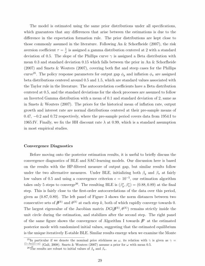
low values of 0.5 and using a convergence criterion ε = 10−5, our estimation algorithm
takes only 5 steps to converge26. The resulting BLE is (β∗y , β∗π) = (0.88, 0.89) at the final
step. This is fairly close to the first-order autocorrelations of the data over this period,
given as (0.87, 0.89). The left panel of Figure 3 shows the norm distances between two
consecutive sets of βββ(k) and θ(k) at each step k, both of which rapidly converge towards 0.
The largest eigenvalue of the Jacobian matrix DG(βββ(k), θ(k)) remains strictly inside the
unit circle during the estimation, and stabilizes after the second step. The right panel
of the same figure shows the convergence of Algorithm I towards βββ∗ at the estimated
posterior mode with randomized initial values, suggesting that the estimated equilibrium
is the unique iteratively E-stable BLE. Similar results emerge when we examine the Monte
25In particular if we denote the nominal price stickiness as ω, its relation with γ is given as γ =(1−λω)(1−ω)
ω (Gali, 2008). Smets & Wouters (2007) assume a prior for ω with mean 0.5.26The results are robust to initial values of βy and βπ.
29
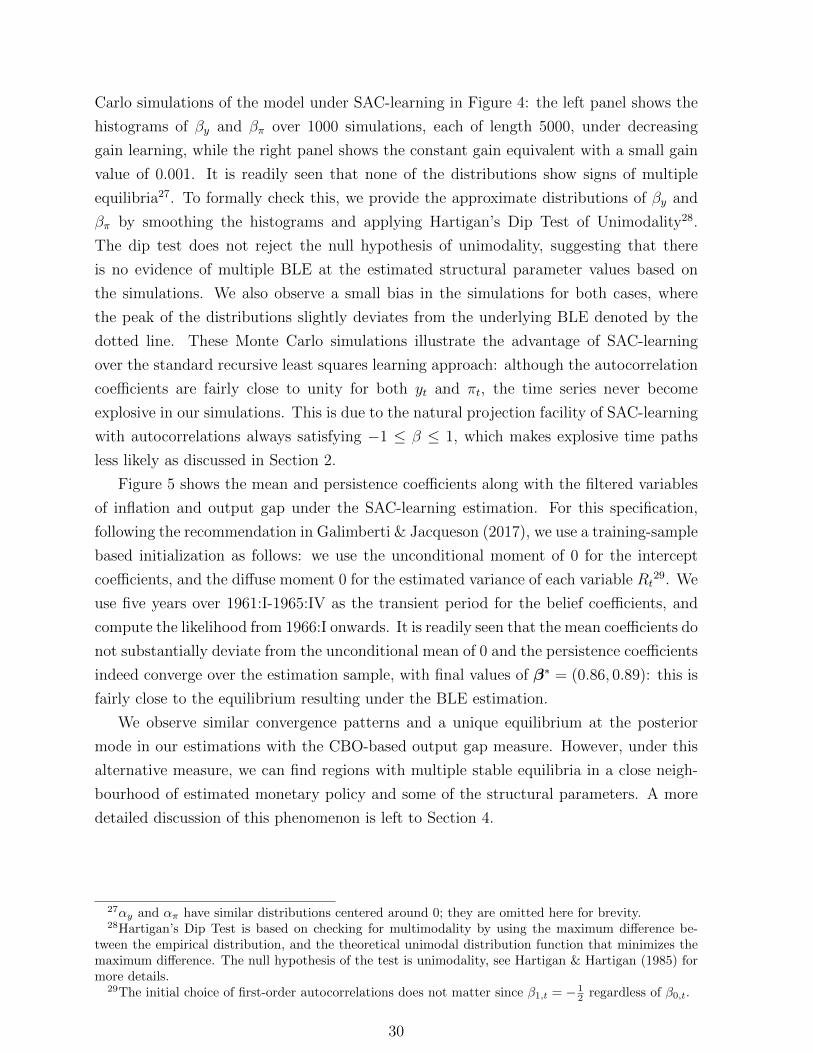
Carlo simulations of the model under SAC-learning in Figure 4: the left panel shows the
histograms of βy and βπ over 1000 simulations, each of length 5000, under decreasing
gain learning, while the right panel shows the constant gain equivalent with a small gain
value of 0.001. It is readily seen that none of the distributions show signs of multiple
equilibria27. To formally check this, we provide the approximate distributions of βy and
βπ by smoothing the histograms and applying Hartigan’s Dip Test of Unimodality28.
The dip test does not reject the null hypothesis of unimodality, suggesting that there
is no evidence of multiple BLE at the estimated structural parameter values based on
the simulations. We also observe a small bias in the simulations for both cases, where
the peak of the distributions slightly deviates from the underlying BLE denoted by the
dotted line. These Monte Carlo simulations illustrate the advantage of SAC-learning
over the standard recursive least squares learning approach: although the autocorrelation
coefficients are fairly close to unity for both yt and πt, the time series never become
explosive in our simulations. This is due to the natural projection facility of SAC-learning
with autocorrelations always satisfying −1 ≤ β ≤ 1, which makes explosive time paths
less likely as discussed in Section 2.
Figure 5 shows the mean and persistence coefficients along with the filtered variables
of inflation and output gap under the SAC-learning estimation. For this specification,
following the recommendation in Galimberti & Jacqueson (2017), we use a training-sample
based initialization as follows: we use the unconditional moment of 0 for the intercept
coefficients, and the diffuse moment 0 for the estimated variance of each variable Rt29. We
use five years over 1961:I-1965:IV as the transient period for the belief coefficients, and
compute the likelihood from 1966:I onwards. It is readily seen that the mean coefficients do
not substantially deviate from the unconditional mean of 0 and the persistence coefficients
indeed converge over the estimation sample, with final values of β∗ = (0.86, 0.89): this is
fairly close to the equilibrium resulting under the BLE estimation.
We observe similar convergence patterns and a unique equilibrium at the posterior
mode in our estimations with the CBO-based output gap measure. However, under this
alternative measure, we can find regions with multiple stable equilibria in a close neigh-
bourhood of estimated monetary policy and some of the structural parameters. A more
detailed discussion of this phenomenon is left to Section 4.
27αy and απ have similar distributions centered around 0; they are omitted here for brevity.28Hartigan’s Dip Test is based on checking for multimodality by using the maximum difference be-
tween the empirical distribution, and the theoretical unimodal distribution function that minimizes themaximum difference. The null hypothesis of the test is unimodality, see Hartigan & Hartigan (1985) formore details.
29The initial choice of first-order autocorrelations does not matter since β1,t = − 12 regardless of β0,t.
30
1 2 3 4 50
0.5
1
1.5
2
ρ(DG(k)
)
||β(k)
-β(k-1)
||
||θ(k)
-θ(k-1)
||
(a) Convergence towards β∗β∗β∗
0 100 200 300 400 5000
0.1
0.2
0.3
0.4
0.5
0.6
0.7
0.8
0.9
1
0 100 200 300 400 5000
0.1
0.2
0.3
0.4
0.5
0.6
0.7
0.8
0.9
1
(b) Iterative E-stability of the unique β∗
Figure 3: The estimated BLE is (β∗y , β∗π) = (0.88, 0.89). The left panel shows the largest
eigenvalue, and the norm distances between consecutive values of β(k)β(k)β(k), as well as θ(k)
across iterations. The second panel shows convergence towards the unique (iteratively)E-stable BLE (β∗y , β
∗π) with randomized initial values.
0.78 0.8 0.82 0.84 0.86 0.88 0.9 0.92 0.94 0.960
0.05
0.1
0.6 0.65 0.7 0.75 0.8 0.85 0.9 0.95 10
0.05
0.1
0.15
0.2
(a) β∗y and β∗π under constant gain learning.
0.75 0.8 0.85 0.9 0.950
0.05
0.1
0.15
0.2
0.6 0.65 0.7 0.75 0.8 0.85 0.9 0.95 10
0.05
0.1
0.15
0.2
(b) β∗y and β∗π under decreasing gain learning.
Figure 4: Monte Carlo Simulations: frequency distributions and unimodality test for βyand βπ resulting from 1000 simulations. Each simulation is of length 5000, initialized atrandom values over the interval (0, 1). Hartigan’s unimodality test p-values are 0.98 and0.94 for βy and βπ under constant gain simulations, and 0.99 and 0.99 for the decreasinggain simulations. Hence the null hypothesis of unimodality is not rejected for any of thedistributions.
31

1965 1970 1975 1980 1985 1990 1995 2000 2005 2010 2015-6
-4
-2
0
2
4Output Gap
Filtered VariableLearning-Mean Coef.
1965 1970 1975 1980 1985 1990 1995 2000 2005 2010 2015-1
0
1
2
3Inflation
(a) Filtered Variables and mean parameters
1965 1970 1975 1980 1985 1990 1995 2000 2005 2010 2015-1
-0.5
0
0.5
1Output Gap
1965 1970 1975 1980 1985 1990 1995 2000 2005 2010 2015-1
-0.5
0
0.5
1Inflation
(b) Persistence parameters
Figure 5: Filtered variables and learning parameters over the estimation sample underSAC-learning, where Kalman filter output is used to update the belief coefficients. Con-verged values of first-order autocorrelations are 0.86 and 0.89 for output gap and inflationrespectively.
Posterior Results: HP-filtered Output Gap
Table 2 presents the posterior estimation results for the REE, BLE and SAC-learning
models.30, where we use the cycle component of the HP-filtered historical output as our
measure of output gap. Starting with a comparison of the BLE and REE results, we
observe several important differences in the estimates of structural parameters: both
persistence parameters for the inflation and output shocks, ρπ and ρy, are substantially
lower under BLE, namely with 0.31 and 0.42 respectively, while they are 0.88 and 0.87
under REE. This is a direct consequence of the difference in the expectation formation
rule. As such, the estimation results confirm the persistence amplification property of
BLE: the backward-looking expectation formation rule endogenously generates additional
inertia for inflation and output gap, which in turn leads to much smaller persistence in
the exogenous shocks. The low autocorrelations in uπ and uy under BLE immediately
imply higher estimated standard deviations for the i.i.d shocks of these AR(1) processes
at 0.29 and 0.73, while these are 0.04 and 0.16 under REE31. Since interest-rate is not
30BLE and REE models are estimated using the Dynare toolbox (Adjemian et. al, 2011), while ourown toolbox is used for the SAC-learning estimations since it requires an additional learning step in thefilter recursions. The posterior distributions are constructed using the Metropolis-Hastings algorithmwith 250000 draws, using the first 50000 as the burn-in sample. The step size for the scale parameterof the jumping distribution’s covariance matrix is adjusted in both models to obtain a rejection rate of70% in both models, which is in the commonly assumed appropriate range for the MH algorithm.
31Note that for an AR(1) process xt = ρxxt−1 + ut, ut ∼ iid(0, σu), the unconditional variance is givenby var(x) = σu
1−ρ2x. This implies, as ρx increases, var(x) also increases.
32

forward-looking, this result does not extend to the interest-rate smoothing ρr, which
is estimated at 0.85 and 0.80 under BLE and REE respectively, while the volatility of
monetary policy shocks is the same at 0.29 under both specifications. The historical
mean parameters turn out fairly similar under both estimations, since they relate to
sample means of the observable variables and are not affected by the expectation rule.
The estimates of monetary policy parameters, φπ and φy, also turn out similar under both
estimations, with 1.36 and 0.48 under BLE, and 1.39 and 0.46 under REE. Finally turning
to the two structural parameters that determine the contemporaneous relation between
the state variables, both the risk aversion coefficient 1ϕ
and the slope of the NKPC γ are
fairly different: these are estimated at 3.02 and 0.035 under BLE, while they are 4.27 and
0.007 under REE respectively. These differences arise due to altered cross-restrictions
under learning: the additional inertia that we introduce under BLE comes at the cost of a
weaker contemporaneous relation between the state variables and shocks. While the state
variables are only related to the shocks through 1ϕ
and γ under BLE, they are also indirecly
related through expectations under REE. As a result, the risk aversion coefficient turns
out lower under learning, implying a larger direct impact from the ex-ante risk premium
on output gap under BLE. Similarly, γ turns out higher under BLE, implying a stronger
direct effect from output gap on inflation. It is also interesting to note that confidence
intervals for γ are almost mutually exclusive under these two specifications, with a lower
bound of 0.015 under BLE and an upper bound of 0.017 under REE32.
An important consequence of a higher Phillips curve slope and a lower risk aversion
coefficient under BLE is on the shock propagation: Figure 6 shows the impulse responses of
output gap and inflation to a monetary policy shock under BLE and REE at the posterior
mode33. The cumulative impact of the shock is larger under BLE, particularly for inflation,
but the initial impact is larger under REE since the shock affects current output gap and
inflation contemporaneously through expectations. Under BLE, the shock takes several
quarters to reach its full impact, leading to hump-shaped responses for both inflation and
output gap. The hump-shaped pattern is consistent with previous experimental evidence
on small forecasting rules (Adam, 2007), as well as with empirical studies in the literature,
where a contractionary monetary policy shock typically leads to hump-shaped decreases
in output and inflation with peaks after one to two years; see e.g. Leeper et al. (1996)
and Christiano et al. (1999). This effect is absent at REE since there no lagged state
variables in the model, and it shows that the persistence amplification at BLE is also
32As noted in the previous section, the first-order coefficients are computed based on the posteriormode values. Therefore for completeness, the discussion and comparison of these results (both in thissection and in the upcoming ones) are based on the posterior mode. It is worth noting that, given thesmall differences across the posterior means and modes, a similar discussion can be easily extended tothe posterior mean.
33Note that the shock size is the same under both specifications in this case, since the estimatedstandard deviation of the monetary policy shock is 0.29 both under BLE and REE
33
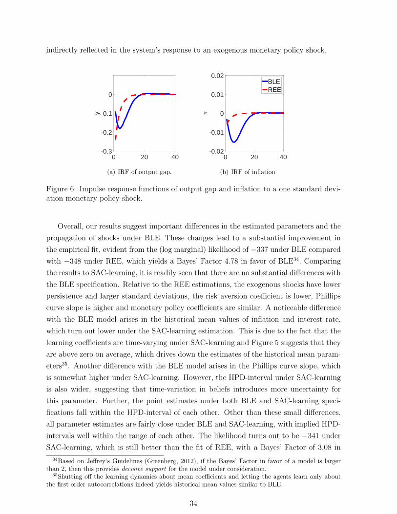
indirectly reflected in the system’s response to an exogenous monetary policy shock.
0 20 40
y
-0.3
-0.2
-0.1
0
(a) IRF of output gap.
0 20 40
:
-0.02
-0.01
0
0.01
0.02BLEREE
(b) IRF of inflation
Figure 6: Impulse response functions of output gap and inflation to a one standard devi-ation monetary policy shock.
Overall, our results suggest important differences in the estimated parameters and the
propagation of shocks under BLE. These changes lead to a substantial improvement in
the empirical fit, evident from the (log marginal) likelihood of −337 under BLE compared
with −348 under REE, which yields a Bayes’ Factor 4.78 in favor of BLE34. Comparing
the results to SAC-learning, it is readily seen that there are no substantial differences with
the BLE specification. Relative to the REE estimations, the exogenous shocks have lower
persistence and larger standard deviations, the risk aversion coefficient is lower, Phillips
curve slope is higher and monetary policy coefficients are similar. A noticeable difference
with the BLE model arises in the historical mean values of inflation and interest rate,
which turn out lower under the SAC-learning estimation. This is due to the fact that the
learning coefficients are time-varying under SAC-learning and Figure 5 suggests that they
are above zero on average, which drives down the estimates of the historical mean param-
eters35. Another difference with the BLE model arises in the Phillips curve slope, which
is somewhat higher under SAC-learning. However, the HPD-interval under SAC-learning
is also wider, suggesting that time-variation in beliefs introduces more uncertainty for
this parameter. Further, the point estimates under both BLE and SAC-learning speci-
fications fall within the HPD-interval of each other. Other than these small differences,
all parameter estimates are fairly close under BLE and SAC-learning, with implied HPD-
intervals well within the range of each other. The likelihood turns out to be −341 under
SAC-learning, which is still better than the fit of REE, with a Bayes’ Factor of 3.08 in
34Based on Jeffrey’s Guidelines (Greenberg, 2012), if the Bayes’ Factor in favor of a model is largerthan 2, then this provides decisive support for the model under consideration.
35Shutting off the learning dynamics about mean coefficients and letting the agents learn only aboutthe first-order autocorrelations indeed yields historical mean values similar to BLE.
34

RE
EB
LE
SA
C
Lap
lace
-348
-337
-341
MH
M-3
48-3
37-3
41
Bay
esF
acto
r1
4.78
3.04
Pri
or
Pos
t.P
ost.
Pos
t.
Para
.D
ist.
Mea
nS
t.D
evM
od
eM
ean
5%
95%
Mod
eM
ean
5%
95%
Mod
eM
ean
5%
95%
σy
Inv.
Gam
ma
0.1
20.
160.
170.
120.
220.
730.
740.
680.
80.
750.
760.
680.
83σπ
Inv.
Gam
ma
0.1
20.
040.
040.
030.
050.
290.
30.
270.
320.
30.
30.
280.
33σr
Inv.
Gam
ma
0.1
20.
290.
30.
280.
330.
290.
290.
270.
320.
290.
290.
270.
32y
Norm
al-0
.20.2
5-0
.15
-0.4
90.
18-0
.12
-0.1
2-0
.40.
17-0
.17
-0.2
1-0
.19
-0.6
0.22
πN
orm
al0.
470.2
50.
70.
710.
530.
90.
790.
790.
670.
910.
410.
450.
180.
75r
Norm
al0.
720.2
50.
980.
980.
711.
261.
11.
090.
851.
320.
650.
70.
331.
06γ
Bet
a0.
30.
150.
007
0.01
0.00
20.
017
0.03
50.
037
0.01
50.
065
0.04
80.
048
0.01
90.
081 ϕ
Gam
ma
20.5
4.27
4.35
3.35
5.37
3.02
3.15
2.33
3.98
2.86
2.98
2.04
3.94
φπ
Gam
ma
1.5
0.2
51.
381.
41.
161.
651.
361.
381.
11.
671.
321.
351.
031.
69φy
Gam
ma
0.5
0.2
50.
480.
510.
340.
670.
490.
520.
310.
730.
480.
510.
290.
76ρy
Bet
a0.
50.
20.
870.
860.
830.
920.
430.
430.
320.
530.
570.
570.
460.
68ρπ
Bet
a0.
50.
20.
880.
870.
820.
910.
320.
320.
220.
430.
250.
260.
140.
38ρr
Bet
a0.
50.
20.
80.
80.
760.
840.
850.
860.
820.
910.
850.
860.
810.
81β∗ y
0.88
0.86
β∗ π
0.89
0.89
Tab
le1:
Post
erio
rre
sult
sw
ith
the
HP
-filt
ered
mea
sure
ofou
tpu
tga
pu
nd
erR
EE
,B
LE
and
SA
C-l
earn
ing
over
the
esti
mat
ion
per
iod
1966
:I-
201
6:IV
.L
apla
cere
fers
toth
eL
apla
ceap
pro
xim
atio
nof
like
lih
ood
bas
edon
the
pos
teri
orm
od
e,w
hil
eM
HM
refe
rsto
the
Mod
ified
Har
mon
icM
ean
esti
mate
ofli
keli
hood
bas
edon
the
pos
teri
ord
istr
ibu
tion
.
35

favor of SAC-learning, but slightly worse than BLE, with a Bayes’ Factor of 1.7 in favor
of BLE36. This result suggests that transitory dynamics and the resulting time-variation
in the learning parameters do not improve the model fit in our decreasing-gain learning
setup. Overall, these results also allow us to illustrate the advantage of using Algorithm II
to estimate a BLE: the estimation under SAC-learning requires a relatively large burn-in
sample for the convergence of first-order autocorrelation coefficients. This might become
an issue if the researcher does not have a sufficiently long dataset, as is typical in most
quarterly macroeconomic time series. Furthermore, as we have already seen in Figure
4, the simulations under learning have a relatively large Monte-Carlo variance. In other
words, while the simulations converge to the underlying BLE on average, there might
be relatively large deviations from the underlying fixed-point for any given simulation.
Hence what comes out of the estimation in a real-time learning setup is similar to a single
simulation of the model under learning, which in general may not accurately reflect the
underlying fixed-point.
Posterior Results: CBO’s Measure of Output Gap
We repeat the estimation exercise for all three specifications under our measure of
output gap derived from CBO’s estimate of potential output37. This measure results
in a time series of output gap that is generally more volatile and has a smaller sample
average38. As a consequence, the estimated historical mean of output gap is lower across
all three specifications compared to the previous section. Under BLE and SAC-learning
specifications, the higher volatility of output gap is reflected in a smaller risk aversion
parameter 1ϕ
(i.e. a larger feedback from the ex-ante real interest rate to output gap),
a smaller Phillips curve coefficient γ and a weaker policy reaction coefficient φy. Under
REE, γ is only marginally smaller and 1ϕ
is actually slightly larger compared to the HP-
filtered measure. Instead, the higher volatility of output gap is reflected in a higher
persistence parameter ρy and a smaller reaction coefficient φy. The remaining parameter
estimates are similar to the previous section under all three specifications, which we do not
discuss in further detail. We also have similar results in terms of the model fit: the (log
marginal) likelihood of BLE and SAC-learning models are −341 and −342 respectively,
compared with −366 under REE. These yield Bayes’ Factors of 10.41 and 10.52 in favor
of BLE and SAC-learning models respectively. In this case, unlike the previous section,
the SAC-learning model yields a slightly better fit than the BLE model, but the difference
is negligible.
36Based on Jeffrey’s Guidelines, this provides very strong evidence in favor of BLE.37See Appendix I for the exact definition of output gap measure used here.38The HP-filter leads to more smoothing compared to CBO-based measure. Therefore downturns
generally have a larger impact under the CBO-based measure, which leads to a lower average and morevolatility in the resulting time series.
36

RE
EB
LE
SA
C
Lap
lace
-366
-342
-341
MH
M-3
66-3
42-3
42
Bay
esF
act
or1
10.4
110
.52
Pri
or
Pos
t.P
ost.
Pos
t.
Par
a.D
ist.
Mea
nS
t.D
evM
od
eM
ean
5%
95%
Mod
eM
ean
5%
95%
Mod
eM
ean
5%
95%
σy
Inv.
Gam
ma
0.1
20.
110.
120.
080.
160.
740.
750.
690.
810.
760.
760.
690.
84σπ
Inv.
Gam
ma
0.1
20.
040.
040.
030.
050.
290.
30.
270.
320.
30.
30.
270.
33σr
Inv.
Gam
ma
0.1
20.
30.
30.
280.
330.
290.
30.
270.
320.
290.
290.
270.
32y
Norm
al-0
.20.2
5-0
.42
-0.4
3-0
.8-0
.04
-0.5
4-0
.53
-0.8
8-0
.17
-0.4
8-0
.49
-0.9
4-0
.05
πN
orm
al0.
470.2
50.
590.
590.
380.
810.
810.
810.
680.
940.
340.
380.
120.
65r
Norm
al0.
720.2
51.
051.
030.
721.
351.
151.
120.
851.
360.
660.
710.
351.
08γ
Bet
a0.
30.
150.
006
0.00
90.
002
0.01
50.
025
0.02
70.
010.
040.
039
0.03
90.
019
0.06
1 ϕG
am
ma
20.5
4.57
4.62
3.61
5.65
2.65
2.78
2.07
3.52
2.38
2.52
1.75
3.4
φπ
Gam
ma
1.5
0.2
51.
421.
471.
21.
731.
411.
441.
121.
771.
451.
471.
111.
83φy
Gam
ma
1.5
0.2
50.
270.
290.
190.
40.
360.
40.
20.
590.
350.
390.
190.
61ρy
Bet
a0.
50.
20.
920.
910.
880.
950.
430.
430.
320.
530.
520.
530.
410.
63ρπ
Bet
a0.
50.
20.
890.
880.
840.
930.
310.
320.
210.
430.
230.
240.
110.
36ρr
Bet
a0.
50.
20.
80.
810.
770.
850.
880.
890.
850.
940.
880.
880.
830.
93β∗ y
0.92
0.94
β∗ π
0.79
0.89
Tab
le2:
Pos
teri
orre
sult
sw
ith
the
CB
O-b
ased
mea
sure
ofou
tpu
tga
pu
nd
erR
EE
,B
LE
and
SA
C-l
earn
ing
over
the
esti
mat
ion
per
iod
1966
:I-
201
6:IV
.L
apla
cere
fers
toth
eL
apla
ceap
pro
xim
atio
nof
like
lih
ood
bas
edon
the
pos
teri
orm
od
e,w
hil
eM
HM
refe
rsto
the
Mod
ified
Har
mon
icM
ean
esti
mate
ofli
keli
hood
bas
edon
the
pos
teri
ord
istr
ibu
tion
.
37

The results presented in this section are generally robust across different subsamples,
as well as with our third measure of output gap based on de-trended output, see Appendix
H for more details. In the following, we analyze monetary policy under BLE.
4 Monetary Policy
Our results show that BLE and SAC-learning generally provide better model fits than
REE for the 3-equation New Keynesian model, with important differences in the estimated
structural parameters and the shock propagation under BLE and REE. This leaves an
important question for the transmission of monetary policy and how it differs under BLE
and REE. In this section, we investigate this issue from two different angles: we first
analyze over which parameter regions multiple BLE exist, and how monetary policy may
mitigate multiplicity of equilibria. We then consider optimal monetary policy under BLE
and REE based on an expected loss function. In both cases, we find important differences
in terms of monetary policy implications under BLE compared to REE. Particularly,
we find that plausible parameter regions with a unique REE may be characterized by
multiple E-stable BLE, and a monetary policy that is optimal under REE may perform
poorly under BLE.
4.1 Multiple Equilibria
Our analysis so far focuses on cases with a unique E-stable BLE. However, in general,
multiple E-stable BLE may coexist. In this section, we provide several examples of how
this phenomenon might occur, and how monetary policy might mitigate multiplicity of
equilibria. For this analysis, we use our parameter estimates at the posterior mode with
the CBO-based measure of output gap: even though the equilibrium is unique at the
posterior mode, we find that two E-stable BLE may coexist when there are small changes
in the monetary policy and some of the structural parameters. We do not observe this
multiplicity when considering the parameter estimates under the HP-filtered measure of
output gap, which will be discussed further below.
As a first example, Figure 7a shows the equilibrium persistence of inflation, β∗π as
a function of the inflation reaction parameter φπ. At the estimated reaction parameter
1.41, there is a unique E-stable equilibrium with β∗π ≈ 0.79 as discussed earlier. If we
decrease the reaction parameter, a second, high-persistence equilibrium becomes E-stable
around φπ = 1.36. There is a small range of values over [1.26, 1.36] for φπ where two E-
stable equilibria coexist, seperated by a third, E-unstable equilibrium39. The coexistence
39The plots in Figure 7 are obtained by using a grid search, where we specify a grid of length 20 overthe unit interval for the initial values of βπ and βy, and a grid of length 100 for each parameter under
38

of two E-stable equilibria occurs with respect to not only φπ, but across a wide range
of parameters. The remaining panels in Figure 7 show three examples of this, where
we project the multiple equilibrium regions for inflation persistence under three different
pairs of parameter values40. Figure 7b shows the multiplicity region, i.e. the blue region,
for both policy reaction parameters φπ and φy over the ranges [1, 2.5] and [0.25, 0.5]
respectively: it is readily seen that the system remains in the low persistence region
as long as both parameters are sufficiently high. If either parameter becomes lower, the
system first enters the multiplicity region, where both low- and high-persistence equilibria
coexist. When the parameters are lowered further, the low-persistence equilibrium loses its
stability. This figure suggests that, in order to avoid the multiplicity and high-persistence
regions, a weaker reaction to one variable requires a more aggressive reaction to the other
variable. For example at φy = 0.4, an inflation reaction of φπ = 1.2 is sufficient to avoid
the multiplicity region, whereas at φy = 0.3, this value increases to φπ = 2.
Figure 7c shows the same analysis with respect to φπ and interest rate smoothing
ρr over the ranges [1, 3.5] and [0.8, 0.95]. We observe that, similar to the previous case,
different values of these two parameters give rise to regions with high- and low-persistence
BLE, separated by a multiplicity region where both equilibria coexist. This figure reveals
that interest rate smoothing is crucial in terms of driving the multiple equilibria results:
for values of ρr < 0.86, the system remains in the low-persistence equilibrium as long
as the Taylor principle of φπ > 1 is satisfied. For values of ρr > 0.91, it is not possible
to avoid the high-persistence region for any values of φπ. In fact, over this region with
high ρr, increasing φπ has the opposite of the desired effect and generates at least one
explosive BLE. As such, our analysis suggests that keeping the interest rate smoothing
parameter sufficiently small is more effective than the inflation reaction parameter in terms
of avoiding multiple equilibria. Finally, 7d illustrates how multiple equilibria may arise
with respect to other structural parameters of the system. For this exercise we use the
shock persistence parameters ρπ and ρy over the ranges [0, 0.4] and [0, 0.9] respectively. In
this case we also obtain the starting point of the multiple equilibrium region, i.e. the blue
region, which is near [0.31, 0.41]. For values of ρπ > 0.31, the system is characterized by
a unique E-stable equilibrium for all values of ρy. Values of ρπ < 0.31 divide the system
into three regions with the low- and high-persistence BLE, separated by the multiple
equilibrium region where both E-stable BLE coexist along with one E-unstable BLE.
This phenomenon is known as a cusp bifurcation: the boundaries of the blue region
consideration. Further, we use the quasi-Newton method to obtain the E-unstable equilibrium in Figure7a since Algorithm I cannot converge to it by construction. The remaining panels are obtained by usingAlgorithm I.
40For this exercise, the remaining parameters are fixed at their estimated posterior mode under theCBO-based measure. Also note that the same analysis holds for output gap persistence, we only presentand discuss inflation persistence here due to space limitations.
39
represent saddle-node bifurcation curves, where an additional E-stable BLE is created.
These saddle-node curves merge at a limiting curve to a cusp bifurcation (Kutnetsov, 2013
p.397).
The analysis above can be extended to other structural parameters of the model: for
example, the slope of the Phillips curve γ also plays a crucial role, where a higher param-
eter leads first to multiplicity and high-persistence regions, then to explosive equilibria
similar to interest rate smoothing. These cases are left to our Online Appendix. Further
note that, if we repeat the analysis in this section under our HP-filtered estimates, we
find no evidence of multiple equilibria in a nearby region. Given our results in this section
and our Online Appendix, the small differences in the estimates of γ ( lower under the
CBO-based measure) and ρr (higher under the CBO-based measure) emerge as the key
drivers of this result.
The important takeaway from this section is that, multiple E-stable BLE coexist in
plausible parameter regions even if the Taylor principle of φπ > 1 is satisfied. This is dif-
ferent than REE, where the Taylor principle ensures the equilibrium uniqueness. In these
multiple equilibrium regions, a sufficiently aggressive monetary policy can de-stabilize the
high-persistence BLE and ensure that the system remains in the low-persistence BLE. In
particular, an interest rate smoothing parameter ρr < 0.85 ensures that multiple E-stable
equilibria do not arise. When a low smoothing parameter is not feasible, sufficiently
aggressive reaction coefficients are able to achieve the same result.
For the remainder of this section, we turn to a comparison of optimal monetary policy
under BLE and REE, for which we use both our baseline calibration from Section 3.2, as
well as our baseline estimation with the HP-filtered output gap from Section 3.3. The key
result in both of these cases is that optimal policy under BLE typically looks different
than REE, even if we consider a parameter space with a unique E-stable BLE.
40

φπ
1 1.1 1.2 1.3 1.4 1.5
βπ
0.72
0.77
0.82
0.87
0.92
0.97
1.02
E-stable
E-unstable
E-stable
(a) Inflation and output gap reactions.
φy
0.25 0.3 0.35 0.4 0.45 0.5
φπ
1
1.5
2
2.5
Unique E-stable
Equilibrium
(Low Persistence)
2 E-stable Equilibria
Unique E-stable
Equilibrium
(High Persistence)
(b) Inflation reaction and interest ratesmoothing.
ρr
0.8 0.85 0.9 0.95
φπ
1
1.5
2
2.5
3
3.5
Non-stationary Equilibria
or No Equilibria
Unique E-stable Equilibrrium
(Low Persistence)
2 E-stable Equilibria
Unique E-stable Equilibrium
(High Persistence)
(c) Inflation reaction and interest ratesmoothing.
ρy
0.1 0.2 0.3 0.4 0.5 0.6 0.7 0.8 0.9
ρπ
0
0.05
0.1
0.15
0.2
0.25
0.3
0.35
0.4
Unique E-stable Equilibrium
(Low Persistence)
Unique E-stable
Equilibrium
(High
Persistence)
2 E-stable Equilibria
Cusp Bifurcation
(d) Shock persistence parameters.
Figure 7: Multiple BLE: the first panel (top left) shows a saddle-node bifurcation withrespect to φπ, where two stable BLE are separated by an unstable BLE over the region[1.26, 1.36]. The remaining panels shows the projections of multiple equilibria over two-dimensional parameter regions. The blue regions correspond to cases where we observetwo coexisting E-stable BLE, whereas the red regions correspond to cases with no E-stableBLE. The red dots correspond to the estimated parameter values under CBO-based outputgap.
4.2 Optimal Policy
4.2.1 Calibrated Parameters
In this section we analyze optimal Taylor rules under BLE and REE. We start by
assuming that the central bank wishes to minimize an expected loss function E[L] in
terms of the discounted sum of weighted squared inflation, output gap and interest rate
E[L] = (1− ϑ)E[Σ∞t=0ϑ
t[ωππ2t + ωyy
2t + ωrr
2t ]]
= ωπσ2π + ωyσ
2y + ωrσ
2r , (4.1)
where ωi, i ∈ π, y, r is the relative weight that the central bank places on inflation,
output gap and interest rate respectively. The stabilization objective for inflation and
output gap is a standard assumption in the literature, see e.g. Boehm and House (2014),
41

BLE
Finite Optimal
Policy
REE
0.5 1.0 1.5 2.0
2
4
6
8
Φy
*
ΦΠ*
Figure 8: Optimal policies at the BLE and at the REE. Parameters are: λ = 0.99, ϕ =1, ρπ = ρy = 0.5, ρr = 0, γ = 0.04, σy = 1, σπ = 0.5 and ωy = 0.1, ωr = 0.05.
Evans and Honkapohja (2003) and Woodford (2003). The weight on interest rate variance
can be motivated by different interpretations: Woodford (1999) and Giannoni (2014)
suggest that it can proxy for welfare costs of transactions and/or an approximation on
the zero lower bound on nominal interest rates, while Caplin and Leahy (1996) suggest
that it can represent a gradual learning process for the central bank that is uncertain
about the consequences of interest rate fluctuations.
Based on our calculations and equations (F.12) and (F.13), the unconditional moments
under BLE are given as
σ2y =
g1
(1 + γϕφπ + ϕφy)2(1− ρ2)(1− ρλ1)(1− ρλ2)(1− λ21)(1− λ2
2)(1− λ1λ2),(4.2)
σ2π =
g2
(1 + γϕφπ + ϕφy)2(1− ρ2)(1− ρλ1)(1− ρλ2)(1− λ21)(1− λ2
2)(1− λ1λ2),(4.3)
σ2r = φ2
yσ2y + φ2
πσ2π + 2φyφπE(ytπt), (4.4)
where g1, g2, λ1, λ2 are given by the equations (3.15)-(3.18), and E(ytπt) is a complicated
expression in terms of the structural parameters and first-order autocorrelations βy and
βπ41.
In the following we study the optimal values (φ∗y, φ∗π) that minimize the central bank’s
loss function (4.1) under BLE and REE.
We first examine monetary policy under BLE and REE at our baseline calibration,
where we use the parameters λ = 0.99, ϕ = 1, γ = 0.04, ρy = ρπ = ρ = 0.5, ρr = 0, σπ =
0.5 and σy = 1 for both BLE and REE. Using this calibration serves two purposes:
first, using the same parameter values under both specifications ensures that the data
generating process only differs in terms of the expectation formation rule. Second, in
41See Appendix F, equation (F.16).
42

0.5 1.0 1.5 2.0
2.08
2.10
2.12
2.14
2.16
2.18
Φy
*
ΣΠ2+Ω
yΣ
y2+Ω
rΣ
r2
(a) At the BLE
0.5 1.0 1.5 2.0
1.35
1.40
1.45
1.50
1.55
Φy
*
ΣΠ2+Ω
yΣ
y2+Ω
rΣ
r2
(b) At the REE
Figure 9: Loss function along the optimal paths (φ∗y, φ∗π) in Figure 8 at the BLE (a) and
REE (b). Parameters are: λ = 0.99, ϕ = 1, , ρπ = ρy = ρ = 0.5, ρr = 0, γ = 0.04, σy =1, σπ = 0.5 and ωy = 0.1, ωr = 0.05.
the absence of interest rate smoothing and given the assumption of ρπ = ρy, we can use
the expressions in (3.13)-(3.18) to evaluate BLE, which allows us to provide some insight
on how optimal monetary policy under BLE depends on model parameters, such as the
persistence of exogenous shocks.
As we saw in previous sections, there are important differences in the moments of
endogenous variables due to volatility and persistence amplification at BLE. In particular,
the implied variances of inflation, output gap and interest rate are different under BLE
and REE at the calibrated parameter values. Following Woodford (1999) and Giannoni
(2014), we normalize the weight on inflation to ωπ = 1. We first focus on a special case
with ωy = 0.1 and ωr = 0.05, that is, the central bank places a relatively large weight on
inflation and a small one on interest rates. The small weight on interest rates allows us to
first focus on the trade-off between inflation and output gap stabilization. We leave the
discussion of how optimal policy depends on these policy weights to the case of estimated
parameter values.
Interestingly, we find that the optimal Taylor rule coefficients (φ∗y, φ∗π) are finite under
BLE42. As shown in Figure 8, the corresponding optimal policy is (φ∗y, φ∗π) = (0.91, 4.88).
This is different from REE, where there is no finite optimal policy except when the weight
42We first select a policy parameter domain (e.g. [0, 100] × [1, 100]) and define a lattice with somesmall step (e.g. 0.01). Then for each lattice point (φy, φπ), we find the BLE (β∗1(φy, φπ), β∗2(φy, φπ)) andthe corresponding central bank’s expected loss function E[L] at the BLE. Finally we interpolate the lossfunction with respect to (φy, φπ) to find the finite optimal values. It is easy to get analytic expressions ofthe variances and optimal policy parameters under REE. In contrast, it is impossible to obtain analyticexpressions of the optimal policy parameters under BLE and therefore we have to rely on numericalapproximations. We find consistent results using different ways to calculate the variances (i.e. based on(4.2) and (4.3) or computing the variances as in Appendix B).
43
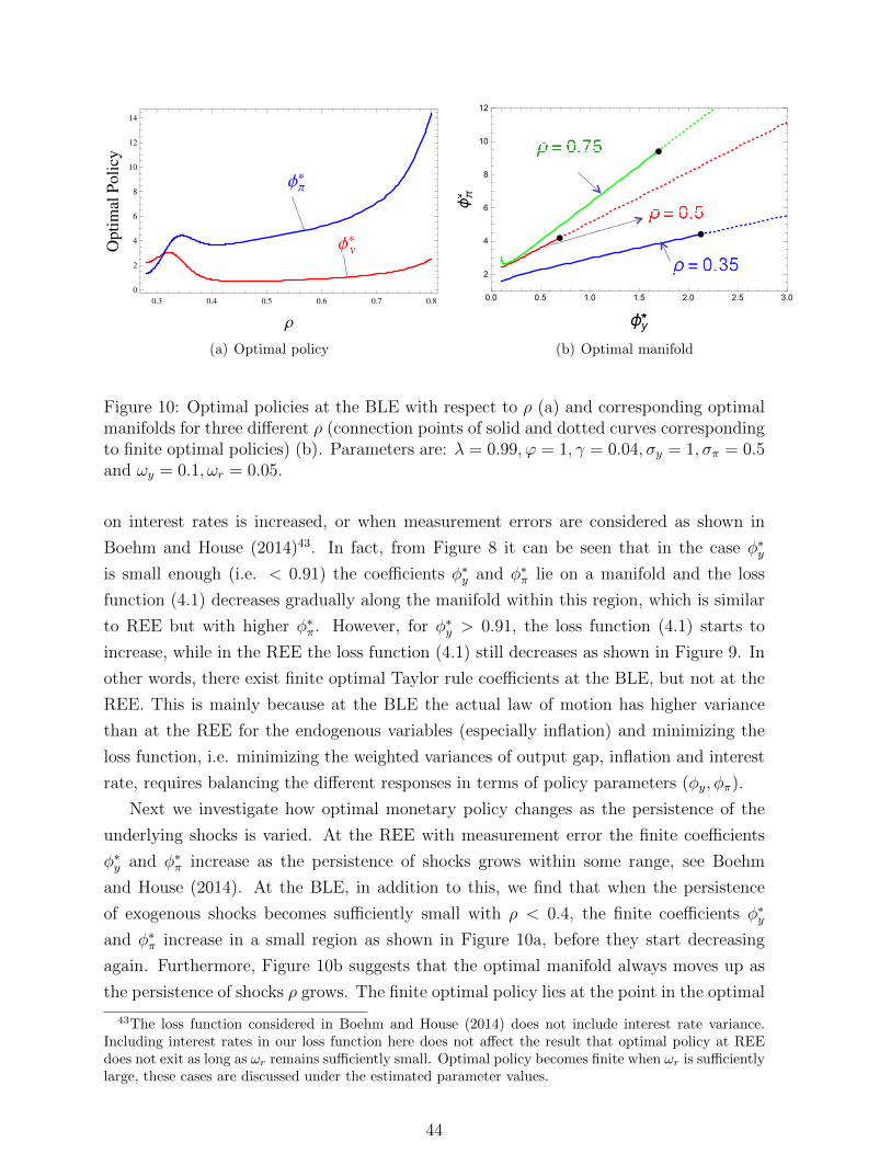
ΦΠ*
Φy
*
0.3 0.4 0.5 0.6 0.7 0.8
0
2
4
6
8
10
12
14
Ρ
Op
tim
alP
oli
cy
(a) Optimal policy
0.0 0.5 1.0 1.5 2.0 2.5 3.0
2
4
6
8
10
12
ϕy
ϕπ
(b) Optimal manifold
Figure 10: Optimal policies at the BLE with respect to ρ (a) and corresponding optimalmanifolds for three different ρ (connection points of solid and dotted curves correspondingto finite optimal policies) (b). Parameters are: λ = 0.99, ϕ = 1, γ = 0.04, σy = 1, σπ = 0.5and ωy = 0.1, ωr = 0.05.
on interest rates is increased, or when measurement errors are considered as shown in
Boehm and House (2014)43. In fact, from Figure 8 it can be seen that in the case φ∗y
is small enough (i.e. < 0.91) the coefficients φ∗y and φ∗π lie on a manifold and the loss
function (4.1) decreases gradually along the manifold within this region, which is similar
to REE but with higher φ∗π. However, for φ∗y > 0.91, the loss function (4.1) starts to
increase, while in the REE the loss function (4.1) still decreases as shown in Figure 9. In
other words, there exist finite optimal Taylor rule coefficients at the BLE, but not at the
REE. This is mainly because at the BLE the actual law of motion has higher variance
than at the REE for the endogenous variables (especially inflation) and minimizing the
loss function, i.e. minimizing the weighted variances of output gap, inflation and interest
rate, requires balancing the different responses in terms of policy parameters (φy, φπ).
Next we investigate how optimal monetary policy changes as the persistence of the
underlying shocks is varied. At the REE with measurement error the finite coefficients
φ∗y and φ∗π increase as the persistence of shocks grows within some range, see Boehm
and House (2014). At the BLE, in addition to this, we find that when the persistence
of exogenous shocks becomes sufficiently small with ρ < 0.4, the finite coefficients φ∗y
and φ∗π increase in a small region as shown in Figure 10a, before they start decreasing
again. Furthermore, Figure 10b suggests that the optimal manifold always moves up as
the persistence of shocks ρ grows. The finite optimal policy lies at the point in the optimal
43The loss function considered in Boehm and House (2014) does not include interest rate variance.Including interest rates in our loss function here does not affect the result that optimal policy at REEdoes not exit as long as ωr remains sufficiently small. Optimal policy becomes finite when ωr is sufficientlylarge, these cases are discussed under the estimated parameter values.
44

manifold connecting the solid and dotted lines in Figure 10b. The location of the optimal
point corresponding to finite optimal policies depends on the relative values of variances
of inflation, output gap and interest rate. In the case where ρ is large enough, the loss
function is mainly dominated by the variance of inflation and hence the optimal policy
φ∗π grows quickly converging to ∞, and the slope of φ∗πφ∗y
converging to a large constant.
As ρ becomes smaller, the variance of interest rate starts to play a more dominant role,
which leads to smaller values for both φ∗π and φ∗y. The region with small values of ρ is
more relevant for U.S. data since both shock persistence parameters are low at the BLE
in our estimation exercises.
These results show that optimal policy exists under BLE for this parameterization,
different than REE, and that the optimal rule (φ∗y, φ∗π) under BLE crucially depends on
the persistence of exogenous shocks.
4.2.2 Estimated Parameters
Next we examine optimal monetary policy for the empirically more relevant case of
estimated parameters. In this case the underlying structural parameters are different at
BLE and REE, but the variances of inflation, output gap and interest rate are close under
these two specifications. In particular, given the estimated parameter values and our
benchmark policy weights of (ωy, ωr) = (0.1, 0.05), the expected loss function E[L] is 0.57
at BLE and 0.55 at REE44. This allows us to compare monetary policy under BLE and
REE with a similar starting point for the loss function.
For this exercise, we limit our attention to Taylor parameters φy and φπ over the range
[0, 15]. In this case we find that optimal monetary policy exists not only at BLE, but also
at REE for a wide range of policy weights45. The difference at REE between calibrated
and estimated parameters is driven by the exogenous shocks, which are estimated to
be highly persistent, and the Phillips curve, which is estimated to be flatter compared
to the calibration. This introduces a larger trade-off between inflation and output gap
stabilization at REE, which leads to a finite optimal policy for a wide range of policy
weights. Given this result, we can compare how the optimal parameters differ at BLE
and REE.
Table 3 shows the optimal Taylor rules for several pairs of (ωy, ωr), along with some
key statistics at BLE and REE. The first two rows show our benchmark calibration of
44Our analysis with calibrated parameter values is based on the expressions (4.2)-(4.4). These expres-sions are no longer applicable for the estimated version of the model since it also includes an interestrate smoothing parameter, and the assumption of the same persistence for the exogenous shocks is re-laxed. Rather, we use the (different) estimated shock persistence parameters. Therefore we proceed bycomputing the BLE and the associated variances for each value of policy parameters using the IterativeE-stability algorithm.
45See our Online Appendix for the optimal parameters at BLE and REE for weights ωy and ωr overthe range [0, 0.25].
45

(0.1, 0.05), while the second row considers a calibration (0.048, 0.236) as in Woodford
(1999) and Giannoni (2014). The remaining two rows show the effects of increasing the
weight on output gap and interest rate relative to the benchmark calibration, where we
consider weights of (0.1, 0.15) and (0.2, 0.05) respectively. Several observations stand out
from the table: first, it is readily seen that optimal policy at BLE is typically more
aggressive in both parameters φ∗π and φ∗y, when the relative weight on interest rates is
large enough. To make this point more clear, Figure 11 shows the optimal parameters
at BLE and REE as a function of the relative weight on interest rates, ωrωy
. When ωrωy
approaches zero, optimal parameters under both BLE and REE quickly start converging
to infinity, whereas when ωrωy
increases, optimal parameters under both BLE and REE
decrease. φ∗y under BLE remains higher than REE across all combinations of weights,
suggesting a more aggressive response to output gap. φ∗π under BLE remains smaller
than REE until ωrωy≈ 1.5, after which the optimal parameter under BLE always remains
larger than REE.
These results suggest that φ∗π under BLE is less sensitive to changes in the policy
weights, while φ∗y under BLE is more sensitive. In other words, optimal policy at REE
responds to changes in policy weights mainly through φ∗π, while optimal policy at BLE
responds to these changes through φ∗y. This result is mainly driven by the estimates of1ϕ
and γ, both of which are larger under BLE: a larger 1ϕ
implies a stronger impact from
interest rates to output gap, while a larger γ implies a stronger impact from output gap
to inflation. As a consequence of this, stabilizing output gap plays a more dominant role
at BLE compared to REE, since the effect of this on inflation is also larger46. A side effect
of this stronger channel at BLE is on the loss function: the columns E[L∗] and ∆E[L∗]
show the value of the loss function at the optimal parameter values, and the percentage
improvement in the loss function compared to the benchmark value of the loss function.
It is readily seen that the improvements achieved under BLE are substantially larger
compared to REE, suggesting a stronger influence on the economy from interest rates.
This is in line with our earlier finding that impulse responses of inflation and output gap
to a monetary policy shock are larger under BLE.
As a final exercise, we consider optimal parameters when the interest rate smoothing
parameter is shut off, which serves two purposes: since the estimated value of interest rate
smoothing is different under BLE and REE, this allows us to compare optimal policies with
an equal rate of smoothing. Second, our results from multiple equilibria section suggest
that excessive interest rate smoothing is undesirable, since it may lead to multiple stable
BLE and even de-stabilize the economy. Here we check whether there are any benefits to
46For the cases where the Taylor rule of φπ > 1 is violated in Table 3, the REE model is still determinatesince the estimated Phillips curve slope is very small. Further, in all cases considered here, we have aunique E-stable BLE since the interest rate smoothing parameter is not excessively large.
46

interest rate smoothing at BLE in the absence of multiple equilibria.
In this case we find optimal parameters under both BLE and REE that are generally
smaller compared to the previous case, which is not surprising since shutting off ρr allows
for larger movements in interest rates, which in turn leads to smaller optimal parameters.
More importantly, this exercise reveals that, while interest rate smoothing is typically
welfare improving at REE, this is never the case at BLE: E[L∗] is uniformly smaller
and ∆E[L∗] uniformly larger at BLE when interest rate smoothing is shut off, while the
opposite holds at REE. The result for REE is well-known from Woodford (1999), where a
commitment to interest rate smoothing has a stabilizing effect with forward-looking agents
who anticipate and take into account future changes in interest rate. This is different
than a BLE with backward-looking agents, where such a commitment does not have a
stabilizing effect since agents are unaware of the commitment or do not take it into account
when forming their expectations. In other words, agents confuse a higher degree of interest
rate smoothing with weaker reactions coefficients in a BLE. An important implication of
this for a central bank is that, not communicating an interest rate smoothing objective
in a credible manner to the public may have welfare decreasing effects.
Overall, our results in this section yield important differences on the effects of monetary
policy under BLE and REE. In particular, we find that (i) multiple E-stable BLE may
coexist in plausible parameter regions typically associated with a unique REE, (ii) optimal
policy at BLE exist in parameter regions where there is no optimal policy at REE, (iii)
optimal parameters are typically different in regions where optimal policy exists for both
BLE and REE. These results imply that a monetary policy that is optimal under REE
may perform poorly under BLE.
!r=!y
2 4 6 8
?:
*
0
5
10
15
(a) φ∗π as a function of ωr
ωy.
!r=!y
2 4 6 8
?y*
0
5
10BLEREE
(b) φ∗y as a function of ωr
ωy.
Figure 11: Changes in optimal parameters as a function of the relative weight on theinterest rate.
47

ωπ ωy ωr BLE REE BLE REEρr = 0.85 ρr = 0.8 ρr = 0.85 ρr = 0.8
φ∗y φ∗π φ∗y φ∗π E[L∗] ∆E[L∗] E[L∗] ∆E[L∗]
1 0.1 0.05 3.94 3.49 2.74 4.43 0.24 58 % 0.40 27 %1 0.048 0.236 1.67 1.56 0.94 0.75 0.34 32 % 0.55 1 %1 0.1 0.15 2.42 1.82 1.25 1.96 0.32 48 % 0.52 15 %1 0.2 0.05 6.67 3.94 2.64 8.51 0.28 68 % 0.41 46 %
ωπ ωy ωr BLE REE BLE REEρr = 0 ρr = 0 ρr = 0 ρr = 0
φ∗y φ∗π φ∗y φ∗π E[L∗] ∆E[L∗] E[L∗] ∆E[L∗]
1 0.1 0.05 1.21 1.67 2.17 4.91 0.24 59 % 0.43 21 %1 0.048 0.236 0.46 0.91 0.38 0.49 0.30 40 % 0.64 -16 %1 0.1 0.15 0.76 1.06 0.62 1.62 0.31 59 % 0.61 1 %1 0.2 0.05 2.12 1.67 2.31 10.36 0.27 69 % 0.43 43 %
Table 3: Optimal Taylor rules and some key statistics at BLE and REE: top panel showsthe results under the estimated parameter values in each case, while the bottom panelshows the same results without interest rate smoothing, i.e. ρr = 0. E[L∗] shows the lossfunction value at the optimal policy, while ∆E[L∗] shows the percentage improvement atthe optimal policy relative to the loss function at the estimated parameters.
5 Concluding Remarks
We have generalized the Behavioral Learning Equilibria concept to an n-dimensional
linear stochastic framework and provided a general iterative method to approximate and
estimate BLE. We have applied our framework to the 3-equation New Keynesian model.
Boundedly rational agents use univariate AR(1) forecasting rules for output gap and in-
flation. A BLE is parameter free, as along the BLE the two parameters of each rule
are pinned down by two observable statistics: the unconditional mean and the first-order
autocorrelation. Hence, along a first-order approximation, the simple linear forecasting
rule is optimal within the class of AR(1) heuristics and consistent with observed re-
alizations. Agents gradually update the two coefficients –sample mean and first-order
autocorrelation– of their linear rule through sample autocorrelation learning. In the long
run, agents thus learn to coordinate on the best univariate linear forecasting rule for
each endogenous state variable, without fully recognizing the more complex structure of
the economy. In higher-dimensional systems, BLE exist under general conditions and we
provide simple stability conditions under learning. In the New Keynesian model without
interest rate smoothing, a BLE always exists when the Taylor Principle is satisfied.
A striking feature of BLE is the strong persistence amplification: the persistence of
output and inflation along a BLE is much higher, often near unit root, than the persis-
tence in the exogenous shocks driving the economy. Estimating the 3-equation model on
historical U.S. data under BLE yields a better model fit and a different shock propagation
compared with the REE model. This leaves an important role for monetary policy with
48
the goal of stabilizing output gap, inflation and interest rates. Different from REE, we
find that multiple E-stable BLE may coexist in plausible parameter regions where the
Taylor principle is satisfied. We find a finite optimal Taylor rule under our benchmark
calibration, unlike REE where no finite policy exists. Furthermore, in parameter regions
where optimal policy exists under REE, we find that the optimal parameters are differ-
ent and typically less aggressive compared to BLE. These results suggest that a monetary
policy that is optimal under REE may perform poorly under BLE. In our follow-up paper,
Hommes et. al. (2019), we extend the estimation of BLE to the more realistic setup of the
medium-scale Smets-Wouters (2007) model, and also consider out-of-sample forecasting
under BLE.
49

Appendix
A Mean of the rational expectations equilibrium
Using (2.10-2.11) and (2.15-2.18) the mean of the REE satisfies
x∗ = (III − ccc1)−1(ccc0 + ccc2uuu)
= (III − ccc1)−1(III − bbb1ccc1 − bbb1)−1(bbb0 + bbb1ccc2aaa) + (III − ccc1)−1ccc2(III − ρρρ)−1aaa
= (III − ccc1)−1(III − bbb1ccc1 − bbb1)−1[bbb0 + (bbb1ccc2(III − ρρρ) + (III − bbb1ccc1 − bbb1)ccc2)(III − ρρρ)−1aaa]
= [(III − bbb1ccc1 − bbb1)(III − ccc1)]−1[bbb0 + bbb3(III − ρρρ)−1aaa]
= (III − bbb1 − bbb2)−1[bbb0 + bbb3(III − ρρρ)−1aaa].
B Autocorrelation in the n-dimensional case
The purpose of this appendix is to show that the first-order autocorrelation coeffi-
cients of the stochastic stationary system (2.24) are continuous functions with respect to
(β1, β2, · · · , βn) and the other related parameters. Rewrite model (2.24) asxxxt − xxx = (bbb1βββ
2 + bbb2)(xxxt−1 − xxx) + bbb3(uuut − uuu) + bbb4vvvt,
uuut − uuu = ρρρ(uuut−1 − uuu) + εεεt.(B.1)
That is, xxxt − xxx = (bbb1βββ
2 + bbb2)(xxxt−1 − xxx) + bbb3ρρρ(uuut−1 − uuu) + bbb3εεεt + bbb4vvvt,
uuut − uuu = ρρρ(uuut−1 − uuu) + εεεt.(B.2)
ΓΓΓ(−1) = E[(xxxt − xxx)(xxxt−1 − xxx)′]
= E[(bbb1βββ
2 + bbb2)(xxxt−1 − xxx)(xxxt−1 − xxx)′ + bbb3ρρρ(uuut−1 − uuu)(xxxt−1 − xxx)′ + bbb3εεεt(xxxt−1 − xxx)′
+bbb4vvvt(xxxt−1 − xxx)′]
= (bbb1βββ2 + bbb2)ΓΓΓ(0) + bbb3ρρρE[(uuut−1 − uuu)(xxxt−1 − xxx)′]
= (bbb1βββ2 + bbb2)ΓΓΓ(0) + bbb3ρρρE[(uuut − uuu)(xxxt − xxx)′]. (B.3)
50
ΓΓΓ(0) = E[(xxxt − xxx)(xxxt − xxx)′]
= E[(bbb1βββ
2 + bbb2)(xxxt−1 − xxx)(xxxt − xxx)′ + bbb3ρρρ(uuut−1 − uuu)(xxxt − xxx)′ + bbb3εεεt(xxxt − xxx)′ + bbb4vvvt(xxxt − xxx)′]
= (bbb1βββ2 + bbb2)ΓΓΓ(1) + bbb3ρρρE[(uuut−1 − uuu)(xxxt − xxx)′] + bbb3E[εεεt(xxxt − xxx)′] + bbb4E[vvvt(xxxt − xxx)′]
= (bbb1βββ2 + bbb2)ΓΓΓ(1) + bbb3ρρρE[(uuut−1 − uuu)(xxxt − xxx)′] + bbb3ΣΣΣεεεbbb
′3 + bbb4ΣΣΣvvvbbb
′4. (B.4)
Note that E[εεεt(xxxt − xxx)′] = E[εεεt((bbb1βββ
2 + bbb2)(xxxt−1 − xxx))′ + εεεt(bbb3ρρρ(uuut−1 − uuu))′ + εεεt(bbb3εεεt)′ +
εεεt(bbb4vvvt)′]
= ΣΣΣεεεbbb′3 and E[vvvt(xxxt − xxx)′] = E
[vvvt((bbb1βββ
2 + bbb2)(xxxt−1 − xxx))′ + vvvt(bbb3ρρρ(uuut−1 − uuu))′ +
vvvt(bbb3εεεt)′ + vvvt(bbb4vvvt)
′]
= ΣΣΣvvvbbb′4.
Based on (B.3), (B.4) and ΓΓΓ(−1) = ΓΓΓ(1)′,
ΓΓΓ(0) = (bbb1βββ2 + bbb2)ΓΓΓ(0)(bbb1βββ
2 + bbb2)′ + (bbb1βββ2 + bbb2)E[(xxxt − xxx)(uuut − uuu)′](bbb3ρρρ)′
+bbb3ρρρE[(uuut−1 − uuu)(xxxt − xxx)′] + bbb3ΣΣΣεεεbbb′3 + bbb4ΣΣΣvvvbbb
′4.
In order to obtain the expression of ΓΓΓ(0), we use column stacks of matrices. Suppose
vec(KKK) is the vectorization of a matrix KKK and ⊗ is the Kronecker product47. Under the
assumption that all the eigenvalues of bbb1βββ2 are inside the unit circle, based on the property
of Kronecker product48, it is easy to see all the eigenvalues of (bbb1βββ2 + bbb2)⊗ (bbb1βββ
2 + bbb2) lie
inside the unit circle and hence [III − (bbb1βββ2 + bbb2)⊗ (bbb1βββ
2 + bbb2)]−1 exist. Therefore,
vec(ΓΓΓ(0)) = [III − (bbb1βββ2 + bbb2)⊗ (bbb1βββ
2 + bbb2)]−1[((bbb3ρρρ)⊗ (bbb1βββ2 + bbb2))vec(E[(xxxt − xxx)(uuut − uuu)′])
+(III ⊗ (bbb3ρρρ))vec(E[(uuut−1 − uuu)(xxxt − xxx)′]) + vec(bbb3ΣΣΣεεεbbb′3 + bbb4ΣΣΣvvvbbb
′4)]. (B.5)
Thus in order to obtain ΓΓΓ(1) and ΓΓΓ(0), we need calculate E[(xxxt−xxx)(uuut−uuu)′] and E[(uuut−1−uuu)(xxxt − xxx)′].
E[(xxxt − xxx)(uuut − uuu)′]
= E[(bbb1βββ
2 + bbb2)(xxxt−1 − xxx)(uuut − uuu)′ + bbb3ρρρ(uuut−1 − uuu)(uuut − uuu)′ + bbb3εεεt(uuut − uuu)′ + bbb4vvvt(uuut − uuu)′]
= E[(bbb1βββ
2 + bbb2)(xxxt−1 − xxx)[(uuut−1 − uuu)′ρρρ′ + εεε′t] + bbb3ρρρ(uuut−1 − uuu)[(uuut−1 − uuu)′ρρρ′ + εεε′t]
+bbb3εεεt[(uuut−1 − uuu)′ρρρ′ + εεε′t] + vvvt[(uuut−1 − uuu)′ρρρ′ + εεε′t]]
= (bbb1βββ2 + bbb2)E[(xxxt−1 − xxx)(uuut−1 − uuu)′]ρρρ′ + bbb3ρρρE[(uuut − uuu)(uuut − uuu)′]ρρρ′ + bbb3ΣΣΣε.
47One property of column stacks is that the column stack of a product of three matrices is vec(ABC) =(C ′⊗A)vec(B). For more details on this and related properties, see Magnus and Neudecker(1988, Chapter2) and Evans and Honkapohja (2001, Section 5.7).
48The eigenvalues of A⊗ B are the mn numbers λrµs, r = 1, 2, · · · ,m, s = 1, 2, · · · , n where λ1, · · · , λmare the eigenvalues of m×m matrix A and µ1, · · · , µn are the eigenvalues of n×n matrix B; see Lancasterand Tismenetsky (1985).
51

Correspondingly,
vec(E[(xxxt − xxx)(uuut − uuu)′])
= [III − ρρρ⊗ (bbb1βββ2 + bbb2)]−1[vec(bbb3ρρρE[(uuut − uuu)(uuut − uuu)′]ρρρ′) + vec(bbb3ΣΣΣε)]
= [III − ρρρ⊗ (bbb1βββ2 + bbb2)]−1[(ρρρ⊗ (bbb3ρρρ))vec(E[(uuut − uuu)(uuut − uuu)′]) + (III ⊗ bbb3)vecΣΣΣε)]
= [III − ρρρ⊗ (bbb1βββ2 + bbb2)]−1[(ρρρ⊗ (bbb3ρρρ))[III − ρρρ⊗ ρρρ]−1 + (III ⊗ bbb3)]vec(ΣΣΣε). (B.6)
Furthermore,
E[(xxxt − xxx)(uuut−1 − uuu)′]
= E[(bbb1βββ
2 + bbb2)(xxxt−1 − xxx)(uuut−1 − uuu)′ + bbb3ρρρ(uuut−1 − uuu)(uuut−1 − uuu)′ + bbb3εεεt(uuut−1 − uuu)′ + bbb4vvvt(uuut−1 − uuu)′]
= (bbb1βββ2 + bbb2)E[(xxxt − xxx)(uuut − uuu)′] + bbb3ρρρE[(uuut − uuu)(uuut − uuu)′].
Thus based on (B.6),
vec(E[(xxxt − xxx)(uuut−1 − uuu)′])
= (III ⊗ (bbb1βββ2 + bbb2))vec(E[(xxxt − xxx)(uuut − uuu)′]) + (III ⊗ (bbb3ρρρ))vec(E[(uuut − uuu)(uuut − uuu)′])
= (III ⊗ (bbb1βββ2 + bbb2))[III − ρρρ⊗ (bbb1βββ
2 + bbb2)]−1[(ρρρ⊗ (bbb3ρρρ))[III − ρρρ⊗ ρρρ]−1 + (III ⊗ bbb3)]vec(ΣΣΣε)
+(III ⊗ (bbb3ρρρ))[III − ρρρ⊗ ρρρ]−1vec(ΣΣΣε). (B.7)
Therefore based on (B.7), the expression of matrix E[(xxxt−xxx)(uuut−1−uuu)′ can be obtained.
Then by transposing the matrix E[(xxxt−xxx)(uuut−1−uuu)′, we obtain vec(E[(uuut−1−uuu)(xxxt−xxx)′]).
Furthermore, combining this with (B.6), we obtain the variance-covariance matrix ΓΓΓ(0)
from (B.5) and ΓΓΓ(1) from (B.3). Based on the properties of matrix operations, it is easy
to see that the entries of matrices ΓΓΓ(0) and ΓΓΓ(1) are continuous functions with respect
to (β1, β3, · · · , βn) and the other related parameters. Thus the first-order autocorrelation
coefficients of the nontrivial stochastic stationary system (2.24) are continuous functions
with respect to (β1, β3, · · · , βn) and the other related parameters.
Zero-mean Special Case
Taking (2.32) as the starting point and assuming γ = 000, we have
St = γ1St−1 + γ2βββ2St−1 + γ3ηt (B.8)
The first-order covariance matrix is given by:
ΓΓΓ(1) = E[StS′t−1] = (γ1 + γ2βββ
2)E[St−1S′t−1] + γ3E[ηtS
′t−1]. (B.9)
52

We have E[ηtS′t−1] = 0, while E[ηt−1S
′t−1] = E[ηt−1((γ1 + γ2βββ
2)St−2 + γ3ηt−1)′] = (γ3ΣηΣηΣη)′.
Further denoting (γ1 + γ2βββ2) = M(βββ), the expression in (B.9) reduces to:
ΓΓΓ(1) = M(βββ)ΓΓΓ(0), (B.10)
with ΓΓΓ(0) the variance-covariance matrix. Taking the variance on both sides of (B.8)
yields:
ΓΓΓ(0) = M(βββ)ΓΓΓ(0)M(βββ)′ + γ3ΣηΣηΣηγ′3. (B.11)
Vectorizing both sides and using V ec(ABC) = (C ′ ⊗ A)V ec(B), the expression above
reduces to:
V ec(ΓΓΓ(0)) = (M(βββ)⊗M(βββ))V ec(ΓΓΓ(0)) + (γ3 ⊗ γ3)V ec(ΣηΣηΣη). (B.12)
Hence
V ec(ΓΓΓ(0)) = [I −M(βββ)⊗M(βββ)]−1(γ3 ⊗ γ3)V ec(ΣηΣηΣη), (B.13)
which yields (2.33).
C Proof of Proposition 2 (stability of SAC-learning
under SAC-learning)
This appendix derives the E-stability conditions for a BLE (ααα∗,βββ∗). Set γt = (1+t)−1.
For the learning dynamics in (2.28) and (2.8)49, since all functions are smooth, the SAC-
learning rule satisfies the conditions (A.1-A.3) of Section 6.2.1 in Evans and Honkapohja
(2001, p.124).
In order to check the conditions (B.1-B.2) of Section 6.2.1 in Evans and Honkapohja
(2001, p.125), we rewrite the system in matrix form by
XXX t = AAA(θθθt−1)XXX t−1 + BBB(θθθt−1)WWW t,
where θθθ′t = (αααt,βββt,RRRt),XXX′t = (1,xxx′t,xxx
′t−1,uuu
′t) and WWW ′
t = (1, vvv′t, εεε′t),
AAA(θθθ) =
0 0 0 0
b0 + b1(I − β2)α + b2ab0 + b1(I − β2)α + b2ab0 + b1(I − β2)α + b2a b1βb1βb1β2 0 b2ρb2ρb2ρ
0 I 0 0
a 0 0 ρρρ
,
49For convenience of theoretical analysis, one can set St−1 = Rt.
53

BBB(θθθ) =
1 0 0
0 I b2
0 0 0
0 0 I
.
Based on the properties of eigenvalues, see e.g. Evans and Honkapohja (2001, p.117), all
the eigenvalues of AAA(θθθ) include 0 (multiple n + 1), the eigenvalues of ρρρ and b1βb1βb1β2. Thus
based on the assumptions, all the eigenvalues of AAA(θθθ) lie inside the unit circle. Moreover,
it is easy to see all the other conditions for Section 6.2.1 of Chapter 6 in Evans and
Honkapohja (2001) are also satisfied.
Since xxxt is stationary, then the limits
σ2i := lim
t→∞E(xi,t − αi)2, σ2
xixi,−1:= lim
t→∞E(xi,t − αi)(xi,t−1 − αi)
exist and are finite. Hence according to Section 6.2.1 of Chapter 6 in Evans and Honkapo-
hja (2001, p.126), the associated ODE is
dααα
dτ= xxx(ααα,βββ)−ααα,
dβββ
dτ= RRR−1[EEE − βΩβΩβΩ] = RRR−1ΩΩΩ[EEEΩΩΩ−1 − βββ],
dRRR
dτ= ΩΩΩ−RRR,
(C.1)
where RRR is a diagonal matrix with the i-th diagonal entry Ri and ΩΩΩ, EEE are also diagonal
matrices as defined in Section 2. As shown in Evans and Honkapohja (2001), a BLE
corresponds to a fixed point of the following ODE (C.2).dααα
dτ= xxx(ααα,βββ)−ααα,
dβββ
dτ= GGG− βββ.
(C.2)
Note that βββ and GGG are both diagonal matrices. The Jacobian matrix of C.2 is, in fact,
equivalent to ((III − bbb1βββ
∗2)−1(bbb1 − III) %%%
000 DDDGGGβββ(βββ∗)− III
),
where DDDGGGβββ is a Jacobian matrix with the (i, j)-th entry ∂Gi∂βj
and the form of matrix
%%% is omitted since it is not needed in the proof. Therefore, if all the eigenvalues of
(III − bbb1βββ∗2)−1(bbb1 − III) have negative real parts, and all the eigenvalues of DDDGGGβββ(βββ∗) have
real parts less than 1, the SAC-learning (αααt,βββt) converges to the BLE (ααα∗,βββ∗) as time t
tends to ∞.
54

D Local Stability Conditions and Kalman Filter with
SAC-learning
Local Stability of Quasi-Newton Iteration
This section studies the convergence of the Quasi-Newton iteration in (2.36). In par-
ticular, we show that the condition ρ(DGβββ(βββ∗)) < 1 is not necessary for local stability.
Note that the iteration is given as
β(k+1)β(k+1)β(k+1) = β(k)β(k)β(k) −DFβββ(β(k)β(k)β(k), θ)−1F (β(k)β(k)β(k), θ), (D.1)
with F (β(k)β(k)β(k), θ) = G(β(k)β(k)β(k), θ) − β(k)β(k)β(k). Defining50 H(βββ) = βββ − DFβββ(βββ)−1F (βββ), we need to
show that H(βββ) is locally stable. Note that:
DHβββ(βββ) = DFβββ(βββ)−2D2βββF (βββ)F (βββ),
with DFβββ(βββ) = DGβββ(βββ)− I and D2βββF (βββ) = D2
βββG(βββ), which implies
DHβββ(βββ) = (DβββG(βββ)− I)−2D2βββG(βββ)(G(βββ)− βββ).
Since βββ∗ = G(βββ∗) at a BLE by definition, it follows that ρ(DHβββ(β∗β∗β∗)) < 1. Hence (D.1) is
locally stable at any BLE βββ∗ and one can find a neighbourhood D around βββ∗ such that:
limk→∞Hk(β(0)β(0)β(0)) = β∗β∗β∗,∀β(0)β(0)β(0) ∈ D. (D.2)
Importantly, this result holds for all E-stable and E-unstable BLE. Therefore the Quasi-
Newton iteration may converge to E-unstable fixed-points.
Local Stability of Algorithm II
This section derives the local stability condition for Algorithm II. We first re-write the
maximization problem to derive the local stability condition. Let (000,β∗β∗β∗) be an iteratively
E-stable fixed-point at the estimated parameter values θ∗. Then the belief parameters β∗β∗β∗
and the structural parameters θ∗ satisfy the following conditions:β∗β∗β∗ = G(β∗β∗β∗, θ∗)
θ∗ = argmaxθ
p(θ|Y1:T ,β∗β∗β∗).
(D.3)
50For the remainder, we omit the dependence of G(β, θ) on the structural parameters θ for ease ofnotation.
55

Since the dataset Y1:T remains fixed at each step of the iteration, the second condition
can be written as:
θ∗ = argmaxθ
p(θ|Y1:T ,β∗β∗β∗) = pm(β∗β∗β∗), (D.4)
for some pm(.). This implies that the estimated structural parameters θ∗ are given as a
function of the equilibrium belief parameters β∗β∗β∗ for a given dataset and likelihood function.
Plugging this back into the first condition yields:
β∗β∗β∗ = G(β∗β∗β∗, pm(β∗β∗β∗)). (D.5)
(D.5) has the same functional form as the fixed-point iteration in (2.35). In this case the
Jacobian matrix at the equilibrium β∗β∗β∗ and θ∗ is given by
DGβββ(β∗β∗β∗) =∂G
∂βββ |β∗β∗β∗,θ∗+∂G
∂θ∗∂θ∗
∂βββ |β∗β∗β∗,θ∗. (D.6)
Note that the first component in (D.6) corresponds to the Jacobian matrix of G(βββ) in
the case with fixed parameters, while the second component appears due to the fact
that the structural parameters also depend on β∗β∗β∗. Further note that, all three partial
derivatives that appear in (D.6) can be numerically evaluated. If the eigenvalue condition
ρ(DG(β∗β∗β∗)) < 1 is satisfied, it follows that β∗β∗β∗ = G(β∗β∗β∗, θ∗) is locally stable under (2.40)
and (2.41).
Kalman Filter with SAC learning
This section describes the Kalman filter algorithm used in the SAC-learning estima-
tions in Section 3.3. The main filter block follows standard steps, and we use the filter
output at the end of each iteration to update the belief parameters. Consider the law of
motion (2.32), which can be rewritten as
St = γt + (γ1 + γ2β2t )St−1 + γ3ηt, (D.7)
where γt = γ+ γ2(αt +β2t αt). Denote by S0|0, P0|0,ααα0,βββ0,RRR0 the initial state vector, state
covariance matrix, initial belief parameters and their initial covariance matrix respectively.
Denoting by L, N and T the number of shocks, forward-looking variables and length of
the dataset respectively, the recursion is given as follows:
56

For t = 1 : T
St|t−1 = γt−1 + (γ1 + γ2β2t−1)St−1|t−1,
Pt|t−1 = (γ1 + γ2β2t−1)Pt−1|t−1(γ1 + γ2β
2t−1)′ + γ3Σηγ
′3,
vt = Yt − φ0 − φ1St|t−1,
Σt = φ1Pt|t−1φ′1,
St|t = St|t−1 + Pt|t−1φ′1Σ−1
t vt,
Pt|t = Pt|t−1φ′1Σ−1
t φ1Pt|t−1,
p(yt|αt−1, βt−1) = −L2ln(2π)− 1
2ln|Σt| − 1
2(v′tΣ
−1t vt)
For i = 1 : N
αi,t = αi,t−1 + 1t+1
(xi,t − αi,t−1),
βi,t = βi,t−1 + 1t+1R−1i,t
[(xi,t − αi,t−1)
(xi,t−1 +
xi,0t+1− t2+3t+1
(t+1)2αi,t−1 − 1
(t+1)2xi,t)
− tt+1βi,t−1(xi,t − αi,t−1)2
],
Ri,t = Ri,t−1 + 1t+1
[tt+1
(xi,t − αi,t−1)2 −Ri,t−1
].
End
End
(D.8)
The resulting likelihood function is combined with the prior distributions to obtain
the posterior distribution that is estimated.
E Eigenvalues of matrix BBBβββ2
This appendix shows the sufficiency condition for the existence of BLE in Corollary
2. The characteristic polynomial of Bβββ2 is given by h(ν) = ν2 + c1ν + c2, where
c1 = −β2y + [γϕ+ λ(1 + ϕφy)]β
2π
1 + γϕφπ + ϕφy, c2 =
λβ2yβ
2π
1 + γϕφπ + ϕφy.
Both of the eigenvalues of Bβββ2 are inside the unit circle if and only if both of the following
conditions hold (see Elaydi, 1999):
h(1) > 0, h(−1) > 0, |h(0)| < 1.
57
It is easy to see h(−1) > 0, |h(0)| < 1 for any βi ∈ [−1, 1]. Note that
h(1) =(1− β2
y)(1− λβ2π) + γϕφπ + ϕφy − (γϕ+ λϕφy)β
2π
1 + γϕφπ + ϕφy,
≥ ϕ[γ(φπ − 1) + (1− λ)φy]
1 + γϕφπ + ϕφy.
Thus if γ(φπ − 1) + (1− λ)φy > 0, then h(1) > 0. Therefore, both eigenvalues of Bβββ2 lie
inside the unit circle for all βi ∈ [−1, 1].
F First-order autocorrelation coefficients of output
gap and inflation
This appendix derives the first-order autocorrelation coefficients for output gap and
inflation in the New-Keynesian model. Define zzzt = xxxt−x. Then in order to obtainGGG(ααα,βββ),
we first calculate EEE(ztz′t−1) and EEE(ztz
′t). Rewrite model (3.12) into its VARMA(1,∞)
representation
zzzt = BβBβBβ2zt−1 +CCC∞∑n=0
ρnεεεt−n. (F.1)
Since both eigenvalues of BβBβBβ2 lie inside the unit circle under the assumption γ(φπ − 1) +
(1− λ)φy > 0 (see Appendix E), then
zzzt = C[ρI−C−1BβBβBβ2C]−1
∞∑n=0
[ρn+1I−C−1(BβBβBβ2)n+1C]εεεt−n.
Note ρ is a scalar number and III is a 2× 2 identity matrix. Based on i.i.d. assumption of
εεεt,
EEEztzzz′t = C[ρI−C−1BβBβBβ2C]−1
∞∑n=0
[ρn+1I−C−1(BβBβBβ2)n+1C]ΣΣΣ[ρn+1I− (C−1(BβBβBβ2)n+1C)′] ·
[ρI− (C−1BβBβBβ2C)′]−1C′, (F.2)
where ΣΣΣ =
[σ2
1 0
0 σ22
].
In the following we try to obtain the expression of the matrix EEEztzzz′t and hence we
first calculate the matrix∑∞
n=0[ρn+1I−C−1(BβBβBβ2)n+1C]ΣΣΣ[ρn+1I− (C−1(BβBβBβ2)n+1C)′] and
C−1(BβBβBβ2)n+1C.
58

Note that
BβBβBβ2 =1
1 + γϕφπ + ϕφy
[β2y ϕ(1− λφπ)β2
π
γβ2y (γϕ+ λ(1 + ϕφy))β
2π
].
BβBβBβ2 has two eigenvalues51
λ1 =[β2y + (γϕ+ λ+ λϕφy)β
2π] +
√[β2y + (γϕ+ λ+ λϕφy)β2
π]2 − 4λβ2yβ
2π(1 + γϕφπ + ϕφy)
2(1 + γϕφπ + ϕφy),
λ2 =[β2y + (γϕ+ λ+ λϕφy)β
2π]−
√[β2y + (γϕ+ λ+ λϕφy)β2
π]2 − 4λβ2yβ
2π(1 + γϕφπ + ϕφy)
2(1 + γϕφπ + ϕφy).
Their corresponding eigenvectors are
P1 =[ ϕ(1− λφπ)β2
π
1 + γϕφπ + ϕφy, λ1 −
β2y
1 + γϕφπ + ϕφy
]′,
P2 =[ ϕ(1− λφπ)β2
π
1 + γϕφπ + ϕφy, λ2 −
β2y
1 + γϕφπ + ϕφy
]′.
Let PPP = [P1, P2]. Then
C−1Bβ2CC−1Bβ2CC−1Bβ2C = C−1PC−1PC−1P
[λ1 0
0 λ2
](((C−1PPP )−1,
where
C−1PC−1PC−1P
=
(1+ϕφy)ϕ(1−λφπ)β2π
1+γϕφπ+ϕφy+ ϕφπ
(λ1 −
β2y
1+γϕφπ+ϕφy
)(1+ϕφy)ϕ(1−λφπ)β2
π
1+γϕφπ+ϕφy+ ϕφπ
(λ2 −
β2y
1+γϕφπ+ϕφy
)−γϕ(1−λφπ)β2
π
1+γϕφπ+ϕφy+(λ1 −
β2y
1+γϕφπ+ϕφy
)−γϕ(1−λφπ)β2
π
1+γϕφπ+ϕφy+(λ2 −
β2y
1+γϕφπ+ϕφy
) =:
[d1 d2
d3 d4
].
Correspondingly
(((C−1PPP )−1 =
1
d1d4 − d2d3
[d4 −d2
−d3 d1
],
51In the special case λ1 = λ2, although BβBβBβ2 is not diagonalizable, the expressions of first-order auto-correlations (3.13) and (3.14) still hold based on the Jordan normal form of matrix BβBβBβ2. Without lossof generality, in the following we assume λ1 6= λ2.
59

where
d1d4 − d2d3 = det(CCC−1P ) = ϕ(1− λφπ)β2π(λ2 − λ1).
Hence
C−1(Bβ2)n+1CC−1(Bβ2)n+1CC−1(Bβ2)n+1C = C−1PC−1PC−1P
[λn+1
1 0
0 λn+12
](C−1P )−1(C−1P )−1(C−1P )−1
=1
d1d4 − d2d3
[d1d4λ
n+11 − d2d3λ
n+12 d1d2(λn+1
2 − λn+11 )
d3d4(λn+11 − λn+1
2 ) d1d4λn+12 − d2d3λ
n+11
].
Thus
ρn+1I − C−1(Bβ2)n+1Cρn+1I − C−1(Bβ2)n+1Cρn+1I − C−1(Bβ2)n+1C =
1
d1d4 − d2d3
[d1d4(ρn+1 − λn+1
1 )− d2d3(ρn+1 − λn+12 ) −d1d2(λn+1
2 − λn+11 )
−d3d4(λn+11 − λn+1
2 ) d1d4(ρn+1 − λn+12 )− d2d3(ρn+1 − λn+1
1 )
].
Therefore
[ρn+1I − C−1(Bβ2)n+1C]Σ[ρn+1I − (C−1(Bβ2)n+1C)′][ρn+1I − C−1(Bβ2)n+1C]Σ[ρn+1I − (C−1(Bβ2)n+1C)′][ρn+1I − C−1(Bβ2)n+1C]Σ[ρn+1I − (C−1(Bβ2)n+1C)′] =1
(d1d4 − d2d3)2
[s1(n+ 1) s2(n+ 1)
s2(n+ 1) s3(n+ 1)
],
where
s1(n+ 1) = σ21[d1d4(ρn+1 − λn+1
1 )− d2d3(ρn+1 − λn+12 )]2 + σ2
2[d1d2(λn+12 − λn+1
1 )]2,
s2(n+ 1) = σ21d3d4(λn+1
2 − λn+11 )[d1d4(ρn+1 − λn+1
1 )− d2d3(ρn+1 − λn+12 )] +
σ22d1d2(λn+1
1 − λn+12 )[d1d4(ρn+1 − λn+1
2 )− d2d3(ρn+1 − λn+11 )],
s3(n+ 1) = σ21[d3d4(λn+1
2 − λn+11 )]2 + σ2
2[d1d4(ρn+1 − λn+12 )− d2d3(ρn+1 − λn+1
1 )]2.
Correspondingly it is natural to have
∞∑n=0
[ρn+1I − C−1(Bβ2)n+1C]Σ[ρn+1I − (C−1(Bβ2)n+1C)′]
∞∑n=0
[ρn+1I − C−1(Bβ2)n+1C]Σ[ρn+1I − (C−1(Bβ2)n+1C)′]∞∑n=0
[ρn+1I − C−1(Bβ2)n+1C]Σ[ρn+1I − (C−1(Bβ2)n+1C)′]
=1
(d1d4 − d2d3)2
[ ∑∞n=0 s1(n+ 1)
∑∞n=0 s2(n+ 1)∑∞
n=0 s2(n+ 1)∑∞
n=0 s3(n+ 1)
]
=1
(d1d4 − d2d3)2
[s∗1 s∗2
s∗2 s∗3
], (F.3)
60
where
s∗1 = σ21
[(d1d4 − d2d3)2 1
1− ρ2− 2d1d4(d1d4 − d2d3)
1
1− ρλ1
+ (d1d4)2 1
1− λ21
+2d2d3(d1d4 − d2d3)1
1− ρλ2
− 2d1d2d3d41
1− λ1λ2
+ (d2d3)2 1
1− λ22
]+σ2
2
[(d1d2)2
( 1
1− λ22
− 2
1− λ1λ2
+1
1− λ21
)], (F.4)
s∗2 = σ21
[d3d4
(d1d4 − d2d3)
( 1
1− ρλ2
− 1
1− ρλ1
)+
d1d4
1− λ21
− d1d4 + d2d3
1− λ1λ2
+d2d3
1− λ22
]+ σ2
2 ·[d1d2
(d1d4 − d2d3)
( 1
1− ρλ1
− 1
1− ρλ2
)+
d1d4
1− λ22
− d1d4 + d2d3
1− λ1λ2
+d2d3
1− λ21
], (F.5)
s∗3 = σ21
[(d3d4)2
( 1
1− λ22
− 2
1− λ1λ2
+1
1− λ21
)]+σ2
2
[(d1d4 − d2d3)2 1
1− ρ2− 2d1d4(d1d4 − d2d3)
1
1− ρλ2
+ (d1d4)2 1
1− λ22
+2d2d3(d1d4 − d2d3)1
1− ρλ1
− 2d1d2d3d41
1− λ1λ2
+ (d2d3)2 1
1− λ21
]. (F.6)
Therefore based on (F.2) and (F.3), we can further obtain the expression of EEEztzzz′t.
Note that
[ρI − C−1(Bβ2)C]−1[ρI − C−1(Bβ2)C]−1[ρI − C−1(Bβ2)C]−1 =1
m
[d1d4(ρ− λ2)− d2d3(ρ− λ1) d1d2(λ2 − λ1)
d3d4(λ1 − λ2) d1d4(ρ− λ1)− d2d3(ρ− λ2)
],
where m = (d1d4 − d2d3)(ρ− λ1)(ρ− λ2), and
C[ρI − C−1(Bβ2)C]−1C[ρI − C−1(Bβ2)C]−1C[ρI − C−1(Bβ2)C]−1 =1
m(1 + γϕφπ + ϕφy)
[k1 k2
k3 k4
],
where
k1 = d1d4(ρ− λ2)− d2d3(ρ− λ1)− ϕφπd3d4(λ1 − λ2), (F.7)
k2 = d1d2(λ2 − λ1)− ϕφπ[d1d4(ρ− λ1)− d2d3(ρ− λ2)], (F.8)
k3 = γ[d1d4(ρ− λ2)− d2d3(ρ− λ1)] + (1 + ϕφy)d3d4(λ1 − λ2), (F.9)
k4 = γd1d2(λ2 − λ1) + (1 + ϕφy)[d1d4(ρ− λ1)− d2d3(ρ− λ2)]. (F.10)
Thus we have
EEEztzzz′t = k ·[
k21s∗1 + 2k1k2s
∗2 + k2
2s∗3 k1k3s
∗1 + (k1k4 + k2k3)s∗2 + k2k4s
∗3
k1k3s∗1 + (k1k4 + k2k3)s∗2 + k2k4s
∗3 k2
3s∗1 + 2k3k4s
∗2 + k2
4s∗3
](F.11)
61

where k = 1(1+γϕφπ+ϕφy)2(d1d4−d2d3)4(ρ−λ1)2(ρ−λ2)2
, s∗i is given in (F.4)-(F.6) and ki is given
in (F.7)-(F.10).
Through complicated calculations52, the variances of output gap and inflations can be
further simplified as
E(y2t ) =
1
k(k2
1s∗1 + 2k1k2s
∗2 + k2
2s∗3)
=1
(1 + γϕφπ + ϕφy)2(1− ρ2)(1− ρλ1)(1− λ21)(1− ρλ2)(1− λ2
2)(1− λ1λ2)σ2
1
[[(1 + λ2β4
π)− 2λβ2π(ρ+ λ1 + λ2) + (1 + λ2β4
π)(ρλ1 + ρλ2 + λ1λ2)]
−ρλ1λ2[(1 + λ2β4π)(ρ+ λ1 + λ2)− 2λβ2
π(ρλ1 + ρλ2 + λ1λ2) + (1 + λ2β4π)ρλ1λ2]
]+σ2
2
[[((ϕφπ)2 + ϕ2β4
π)− 2ϕφπϕβ2π(ρ+ λ1 + λ2) + ((ϕφπ)2 + ϕ2β4
π)(ρλ1 + ρλ2 + λ1λ2)]
−ρλ1λ2[((ϕφπ)2 + ϕ2β4π)(ρ+ λ1 + λ2)− 2ϕφπϕβ
2π(ρλ1 + ρλ2 + λ1λ2)
+((ϕφπ)2 + ϕ2β4π)ρλ1λ2]
], (F.12)
E(π2t ) =
1
k(k2
3s∗1 + 2k3k4s
∗2 + k2
4s∗3)
=1
(1 + γϕφπ + ϕφy)2(1− ρ2)(1− ρλ1)(1− λ21)(1− ρλ2)(1− λ2
2)(1− λ1λ2)σ2
1
[γ2[1 + ρλ1 + ρλ2 + λ1λ2 − ρλ1λ2(ρ+ λ1 + λ2)− (ρλ1λ2)2]
]+σ2
2
[[((1 + ϕφy)
2 + β4y)− 2(1 + ϕφy)β
2y(ρ+ λ1 + λ2) + ((1 + ϕφy)
2 + β4y)
(ρλ1 + ρλ2 + λ1λ2)]− ρλ1λ2[((1 + ϕφy)2 + β4
y)(ρ+ λ1 + λ2)− 2(1 + ϕφy)β21 ·
(ρλ1 + ρλ2 + λ1λ2) + ((1 + ϕφy)2 + β4
y)ρλ1λ2]]. (F.13)
Note that here E(y2t ) and E(π2
t ) in fact depend on the trace λ1 + λ2 and determinant
λ1λ2.
With the expression of covariance matrix EEEztzzz′t, in order to obtain the expressions
of first-order autocorrelation coefficient of output gap and inflation, we need to further
calculate the first-order autocovariance EEEztzzz′t−1.
Following the similar calculations to EEEztzzz′t, we can obtain
EEEztzzz′t−1 = C[ρI−C−1BβBβBβ2C]−1
∞∑n=1
[ρn+1I−C−1(BβBβBβ2)n+1C]ΣΣΣ[ρnI− (C−1(BβBβBβ2)nC)′] ·
[ρI− (C−1BβBβBβ2C)′]−1C′
= k
[k2
1w∗1 + k1k2(w∗2 + w∗3) + k2
2w∗4 k1k3w
∗1 + k1k4w
∗2 + k2k3w
∗3 + k2k4w
∗4
k1k3w∗1 + k2k3w
∗2 + k1k4w
∗3 + k2k4w
∗4 k2
3w∗1 + k3k4(w∗2 + w∗3) + k2
4w∗4
],
52Because of limit of pages, we drop the calculations here.
62
where k, ki are given in (F.11) and (F.7)-(F.10), and
w∗1 = σ21
(d1d4 − d2d3)2 ρ
1− ρ2− d1d4(d1d4 − d2d3)
ρ+ λ1
1− ρλ1
+ (d1d4)2 λ1
1− λ21
+d2d3(d1d4 − d2d3)ρ+ λ2
1− ρλ2
− d1d2d3d4λ1 + λ2
1− λ1λ2
+ (d2d3)2 λ2
1− λ22
+σ2
2(d1d2)2[ λ2
1− λ22
− λ1 + λ2
1− λ1λ2
+λ1
1− λ21
],
w∗2 = σ21d3d4
(d1d4 − d2d3)
[ ρ
1− ρλ2
− ρ
1− ρλ1
]+d1d4λ1
1− λ21
− d1d4λ1 + d2d3λ2
1− λ1λ2
+d2d3λ2
1− λ22
+σ2
2d1d2
(d1d4 − d2d3)
[ λ1
1− ρλ1
− λ2
1− ρλ2
]+d2d3λ1
1− λ21
− d1d4λ1 + d2d3λ2
1− λ1λ2
+d1d4λ2
1− λ22
,
w∗3 = σ21d3d4
(d1d4 − d2d3)
[ λ2
1− ρλ2
− λ1
1− ρλ1
]+d1d4λ1
1− λ21
− d1d4λ2 + d2d3λ1
1− λ1λ2
+d2d3λ2
1− λ22
+σ2
2d1d2
(d1d4 − d2d3)
[ ρ
1− ρλ1
− ρ
1− ρλ2
]+d1d4λ2
1− λ22
− d1d4λ2 + d2d3λ1
1− λ1λ2
+d2d3λ1
1− λ21
,
w∗4 = σ21(d3d4)2
[ λ2
1− λ22
− λ1 + λ2
1− λ1λ2
+λ1
1− λ21
]+ σ2
2
(d1d4 − d2d3)2 ρ
1− ρ2
−d1d4(d1d4 − d2d3)ρ+ λ2
1− ρλ2
+ (d1d4)2 λ2
1− λ22
+ d2d3(d1d4 − d2d3)ρ+ λ1
1− ρλ1
−d1d2d3d4λ1 + λ2
1− λ1λ2
+ (d2d3)2 λ1
1− λ21
.
Again through technical calculations, the first-order auto-covariances of output gap
and inflations are further simplified as
E(ytyt−1) =1
k(k2
1w∗1 + k1k2(w∗2 + w∗3) + k2
2w∗4)
=1
(1 + γϕφπ + ϕφy)2(1− ρ2)(1− ρλ1)(1− λ21)(1− ρλ2)(1− λ2
2)(1− λ1λ2)σ2
1
[(ρ+ λ1 + λ2 − λβ2
π)[1− λβ2π(ρ+ λ1 + λ2)] + [λβ2
π(ρλ1 + ρλ2 + λ1λ2)−
ρλ1λ2][(ρλ1 + ρλ2 + λ1λ2)− λβ2πρλ1λ2]
]+ σ2
2
[(ϕφπ(ρ+ λ1 + λ2)− ϕβ2
π))
[ϕφπ − ϕβ2π(ρ+ λ1 + λ2)] + [ϕβ2
π(ρλ1 + ρλ2 + λ1λ2)− ϕφπρλ1λ2]
[ϕφπ(ρλ1 + ρλ2 + λ1λ2)− ϕβ2πρλ1λ2]
], (F.14)
63

E(πtπt−1) =1
k(k2
3w∗1 + k3k4(w∗2 + w∗3) + k2
4w∗4)
=1
(1 + γϕφπ + ϕφy)2(1− ρ2)(1− ρλ1)(1− λ21)(1− ρλ2)(1− λ2
2)(1− λ1λ2)σ2
1
[γ2[(ρ+ λ1 + λ2)− ρλ1λ2(ρλ1 + ρλ2 + λ1λ2)]
]+ σ2
2
[[(1 + ϕφy)(ρ+ λ1 + λ2)− β2
y ] ·
[(1 + ϕφy)− β2y(ρ+ λ1 + λ2)] + [β2
y(ρλ1 + ρλ2 + λ1λ2)− (1 + ϕφy)ρλ1λ2] ·
[(1 + ϕφy)(ρλ1 + ρλ2 + λ1λ2)− β2yρλ1λ2]
]. (F.15)
Therefore, the first-order autocorrelation coefficients of output gap and inflation
G1(βy, βπ) =E(ytyt−1)
E(y2t )
, G2(βy, βπ) =E(πtπt−1)
E(π2t )
,
i.e. the equations (3.13-3.18). Finally, the covariance between output gap and inflation is
given as
E(ytπt) =(− σ2
yγ(− (1 + γϕφπ + ϕφy)(1 + γϕφπ + ϕφy + β2
yρ) + β4πλ(1 + γϕφπ
+ϕφy + β2yρ)(λ+ γϕ+ λϕφy) + β2
πρ[β4yλ+ β2
yλρ(1 + γϕφπ + ϕφy) + γϕ
(−1 + λφπ)(1 + γϕφπ + ϕφy)]− β2yβ
6πλ
2ρ(β2yλ+ ρ(λ+ γϕ+ λϕφy))
)+ σ2
πϕ(− φπ(1 + γϕφπ + ϕφy)[−β4
y − β2yγρϕφπ + (1 + ϕφy)(1 + γϕφπ + ϕφy)] + β2
yβ6πλρ
[−γϕ(−β2y + ρ+ ρϕφy) + λρ(β4
y − (1 + ϕφy)2)] + β4
π
(γϕ(1− β2
yρ+ ϕφy)(1 + γϕφπ
+ϕφy) + λ(−1 + β2yρ− ϕ(γφπ + φy))(β
4y − (1 + ϕφy)
2) + β2yλ
2ρφπ(−β4y +
(1 + ϕφy)2))
+ β2πρ[−β6
yλρφπ + β2yλρφπ(1 + ϕφy)(1 + γϕφπ + ϕφy)− (−1 + λφπ)
(1 + ϕφy)2(1 + γϕφπ + ϕφy) + β4
y(−1− ϕ(γφπ + ϕy) + λ(φπ + ϕφπφy))]))/(
(−1 + ρ2)(−1 + β2yβ
2πλ− ϕ(γφπ + φy))(1 + β2
yρ(−1 + β2πλρ) + γϕφπ + ϕφy
−β2πρ(λ+ γϕ+ λϕφy))
(β4y(−1 + β4
πλ2) + 2β2
yβ2πγϕ(−1 + λφπ) + (1 + γϕφπ + ϕφy)
2
−β4π(λ+ γϕ+ λϕφy)
2)). (F.16)
G Stability for the Taylor rule
This appendix shows the E-stability condition in Corollary 3. Based on Proposition
2, we only need to show that both of the eigenvalues of (III −BBBβββ2)−1(BBB−III) have negative
real parts if γ(φπ − 1) + (1− λ)φy > 0.
The characteristic polynomial of (III −BBBβββ2)−1(BBB− III) is given by h(ν) = ν2− c1ν + c2,
where c1 is the trace and c2 is the determinant of matrix (III − BBBβββ2)−1(BBB − III). Direct
64

calculation shows that
c1 =−(1− λ)(1− β2
y)− 2ϕ(γφπ + φy) + ϕ(γ + λφy)(1 + β2π)
M (1 + γϕφπ + ϕφy), (G.1)
c2 =ϕ[γ(φπ − 1) + (1− λ)φy]
M (1 + γϕφπ + ϕφy), (G.2)
where M=(1−β2
y)(1−λβ2π)+γϕφπ+ϕφy−(γϕ+λϕφy)β2
π
1+γϕφπ+ϕφy.
Both of the eigenvalues of (III −BBBβββ2)−1(BBB − III) have negative real parts if and only if
c1 < 0 and c2 > 0 (these conditions are obtained by applying the Routh-Hurwitz criterion
theorem; see Brock and Malliaris, 1989). If γ(φπ − 1) + (1− λ)φy > 0, from Appendix E
it is easy to see M> 0. Furthermore,
c1 ≤−2ϕ[(γ(φπ − 1) + (1− λ)φy]
M (1 + γϕφπ + ϕφy)< 0, c2 > 0.
H Robustness Checks
This appendix provides some robustness checks on our estimations by considering
subsamples of our main dataset and using a third alternative definition of output gap
based on de-trended output.
Subsample Estimations
We first chek whether our main results hold across different sample periods. To this
end, we use our HP-filtered measure of output gap and consider three periods: 1966:I-
1979:II, the period before Great Moderation; 1966:I-2008:IV, the period before Great
Recession (i.e. before the zero lower bound episode); and 1984:I-2008:IV, the Great
Moderation period.
Table 4 reports the posterior mode and the corresponding Laplace approximation for
all periods under BLE and REE. It is readily seen that the difference between parameter
estimates are preserved across all three periods: BLE is characterized by lower persistence
but larger standard deviation estimates in shocks, a steeper Phillips curve characterized
by larger γ, and a smaller risk aversion coefficient. The estimation under BLE provides a
better model fit under all three subsamples, with Bayes’ Factors of 1.67, 3.93 and 2.44 in
favor of the BLE model.
65

Period 66:I-79:II 66:I-08:IV 84:I-08:IV
BLE REE BLE REE BLE REELaplace -118.63 -122.47 -313.16 -322.10 -34.32 -39.93Bayes Factor 1.67 3.93 2.44
Parameter Mode Mode Mode
ηy 0.94 0.24 0.76 0.17 0.53 0.09ηπ 0.38 0.06 0.3 0.04 0.18 0.08ηr 0.20 0.20 0.31 0.32 0.15 0.15y -0.22 -0.14 -0.09 -0.14 0.05 -0.14π 0.93 0.75 0.84 0.71 0.61 0.58r 1.03 0.86 1.25 1.08 1.14 0.97γ 0.054 0.01 0.033 0.006 0.046 0.0071ϕ
2.44 2.77 4.03 3.78 2.82 3.15
φπ 1.03 1.07 1.29 1.31 1.55 1.57φy 0.39 0.36 0.45 0.42 0.48 0.54ρy 0.5 0.87 0.42 0.88 0.44 0.94ρπ 0.31 0.85 0.32 0.87 0.24 0.55ρr 0.72 0.68 0.83 0.77 0.9 0.85
Table 4: Comparison of the sub-sample estimations under BLE and REE: 66:I-79:II, theperiod before Great Moderation; 66:I-08:IV, the period before Great Recession and thezero lower bound episode; and 84:I-08:IV, the Great Moderation period.
Alternative Definition of Output Gap: Based on De-trended Output
Next we repeat our estimations using a third alternative measure of output gap based
on de-trended output. The estimations over the main sample are reported in Table 5,
which also includes the CBO-based estimates for reference. It is readily seen that the
conclusions from this exercise are similar: BLE is characterized by lower persistence but
larger standard deviation estimates in shocks, a steeper Phillips curve characterized by
larger γ, and a smaller risk aversion coefficient. The likelihood is also better under BLE,
with a Bayes’ Factors of 11.49. Comparing the BLE estimates under de-trended and
CBO-based measures, we observe mainly similar measures with a few exeptions: with
the de-trended measure, we have a slightly lower γ and φy, while 1ϕ
and ηy are slightly
higher. This suggests that the de-trended measure of output gap is even more volatile
than CBO-based measure, which in turn is more volatile than the HP-filtered measure
based on our results in Section 3.
As a final check, we compare the likelihoods across the three sub-samples with these
two measures of output gap, which is reported in Table 6: it is readily seen that the
likelihood under BLE is better for both measures under all sub-samples, although the
difference for the Great Moderation period 1985-I:2008:IV is much smaller. These results
are consistent with our previous findings.
66

BLE det. REE det. BLE CBO. REE CBO.Laplace -360.96 -387.42 -342.9 -366.88Bayes Factor 11.49 10.41
Post. Post.Parameter Mode Mode Mode Modeηy 0.78 0.08 0.74 0.11ηπ 0.3 0.04 0.29 0.04ηr 0.3 0.31 0.29 0.3y -0.13 -0.19 -0.54 -0.42π 0.79 0.66 0.81 0.59r 1.09 0.92 1.15 1.05γ 0.017 0.004 0.024 0.0061ϕ
2.92 4.86 2.65 4.57
φπ 1.44 1.45 1.41 1.43φy 0.22 0.16 0.36 0.27ρy 0.42 0.88 0.42 0.89ρπ 0.31 0.94 0.31 0.92ρr 0.88 0.79 0.88 0.8
Table 5: Alternative estimations of the 3-equation NKPC model: we compare the resultsunder BLE and REE with two alternative specifications of output gap. In the first caseoutput gap is defined as the deviation of output from a quadratic trend, while in the latterwe take the output gap based on CBO’s measure of potential output.
66:I-79:II 66:I-08:IV 84:I-08:IV
BLE REE BLE REE BLE REE
CBO’s estimate -126.07 -127.6 -321.9 -344.4 -36.7 -46.9Bayes Factor 0.66 9.77 4.43
Detrended output -129.9 -133.1 -333.1 -353.2 -48.4 -66.9Bayes Factor 1.39 8.73 8.03
Table 6: Sub-sample estimations with alternative definitions of output gap.
I Data Appendix
This appendix describes the dataset used in our estimations. The observable variables
used in our estimations follow the definitions in Smets & Wouters (2007). Accordingly:yobst = 100log(GDPC09t/LNSindext)
πobst = 100log( GDPDEF09tGDPDEF09t−1
)
robst = 100log(Fundst4
)
(I.1)
67

where the time series are given as:
GDPC09: Real GDP, Billions of Chained 2009 Dollars, Seasonally Adjusted Annual
Rate. Source: Federal Reserve Economic Data (FRED).
GDPDEF09: GDP-Implicit Price Deflator, 2009=100, Seasonally Adjusted. Source:
FRED.
LNU00000000:Unadjusted civilian noninstitutional population, Thousands, 16 years&
over. Source: U.S. Bureau of Labor Statistics (BLS)
LNS10000000: Civilian noninstitutional populations, Thousands, 16 years & over, Sea-
sonally Adjusted.
Source: BLS.
LNSindex = LNS10000000LNS10000000(1992:03)
Source: FRED.
Funds:Federal Funds Rate, Daily Figure Averages in Percentages. Source: FRED.
The observable variable xobst for the output gap in our main estimations is based on
the HP-filtered series of yobst , while the CBO-based output gap is defined as: xt =
100GDPC09−GDPPOTGDPPOT
with GDPPOT53: CBO’s Estimate of the Potential Output, Billions of Chained 2009
Dollars, Not Seasonally Adjusted Quarterly Rate. Source: FRED.
References
[1] Adam, K., 2003. Learning and equilibrium selection in a monetary overlapping gener-
ations model with sticky prices. Review of Economic Studies 70, 887-907.
[2] Adam, K., 2007. Experimental evidence on the persistence of output and inflation.
Economic Journal 117, 603-636.
[3] Adam, K. and Marcet, A., 2011. Internal rationality, imperfect market knowledge and
asset prices. Journal of Economic Theory, 146(3), pp.1224-1252.
[4] Adjemian, S., Bastani, H., Juillard, M., Mihoubi, F., Perendia, G., Ratto, M., &
Villemot, S. 2011. Dynare: Reference manual, version 4.
[5] An, S., & Schorfheide, F. 2007. Bayesian analysis of DSGE models. Econometric
reviews, 26(2-4), 113-172.
53In order to calculate the potential output, CBO uses the theoretical framework in a standard Solowgrowth model setup, see CBO (2001) for more details.
68

[6] Assenza, T., Heemeijer, P., Hommes, C. and Massaro, D., 2014. Individual Expecta-
tions and Aggregate Macro Behavior. CeNDEF Working Paper, University of Amster-
dam.
[7] Boehm, C.E., House, C.L., 2014. Opitmal Taylor rules in New keynesian models.
NBER Working Paper Series: w20237.
[8] Boivin, J., Giannoni, M., 2006. Has monetary policy become more effective? The
Review of Economics and Statistics 88 (3), 445-462.
[9] Branch, W.A., 2006. Restricted perceptions equilibria and learning in macroeconomics,
in: Colander, D. (Ed.), Post Walrasian Macroeconomics: Beyond the Dynamic Stochas-
tic General Equilibrium Model. Cambridge University Press, New York, pp. 135-160.
[10] Branch, W.A., Evans, G.W., 2010. Asset return dynamics and learning. The Review
of Financial Studies 23 (4), 1651-1680.
[11] Bray, M., 1982. Learning, estimation, and the stability of rational expectations. Jour-
nal of economic theory, 26(2), pp.318-339.
[12] Brock, W.A., Malliaris, A.G., 1989. Differential Equations, Stability and Chaos in
Dynamic Economics. North-Holland, Amterdam.
[13] Bullard, J., 2006. The learnability criterion and monetary policy. Federal Reserve
Bank of St. Louis Review 88, 203-217.
[14] Bullard, J., Evans, G.W., Honkapohja, S., 2008. Monetary policy, judgment and
near-rational exuberance. American Economic Review 98, 1163-1177.
[15] Bullard, J., Mitra, K., 2002. Learning about monetary policy rules. Journal of Mon-
etary Economics 49, 1105-1129.
[16] Caplin, A. and Leahy, J., 1996. Monetary policy as a process of search. The American
Economic Review, pp.689-702.
[17] Cho, I.K., Kasa, K., 2014. Learning and model validation. Review of Economic Stud-
ies 82, 45-82.
[18] Cho, In-Koo, and Kenneth Kasa., 2017. Gresham’s Law of Model Averaging. Amer-
ican Economic Review 107.11: 3589-3616.
[19] Christiano, L. J., Eichenbaum, M., & Evans, C. L., 1999. Monetary policy shocks:
What have we learned and to what end?. Handbook of macroeconomics, 1, 65-148.
69

[20] Chung, H., Xiao, W., 2014. Cognitive consistency, signal extraction and macroeco-
nomic persistence. Working Paper Binghamton University.
[21] Clarida, R., Galı, J., Gertler, M., 1999. The science of monetary policy: a New
Keynesian perspective. Journal of Economic Literature 37, 1661-1707.
[22] Clark, T., West, K., 2007. Approximately normal tests for equal predictive accuracy
in nested models. Journal of Econometrics 138, 291-311.
[23] Christiano, L.J., Eichenbaum, M., Evans, C.L., 2005. Nominal rigidities and the
dynamic effects of a shock to monetary policy. Journal of Political Economy 113 (1).
[24] DeCanio, S.J., 1979. Rational expectations and learning from experience. The quar-
terly journal of economics, 93(1), pp.47-57.
[25] Elaydi, S.N., 1999. An Introduction to Difference Equations, 2nd edition. Springer,
New York.
[26] Enders, W., 2010. Applied Econometric Time Series (3rd ed.). John Wiley & Sons,
Inc., USA.
[27] Estrella, A., & Fuhrer, JC, 2002. Dynamic inconsistencies: Counterfactual impli-
cations of a class of rational-expectations models. American Economic Review ,92(4),
1013-1028.
[28] Eusepi, Stefano, and Bruce Preston, 2011. Expectations, learning, and business cycle
fluctuations. American Economic Review 101.6: 2844-72.
[29] Evans, G., 1985. Expectational stability and the multiple equilibria problem in linear
rational expectations models. The Quarterly Journal of Economics, 100(4), pp.1217-
1233.
[30] Evans, G.W., Honkapohja, S., 2001. Learning and Expectations in Macroeconomics.
Princeton University Press, Princeton.
[31] Evans, G.W., Honkapohja, S., 2003. Expectations and the stability problem for op-
timal monetary policies. The Review of Economic Studies 70, 807-824.
[32] Evans, G.W., Honkapohja, S., 2013. Learning as a rational foundation for macroe-
conomics and finance. In: Roman Frydman and Edmund S. Phelps (Eds.), Rethinking
Expectations: The Way Forward for Macroeconomics (Chapter 2). Princeton University
Press.
70

[33] Farmer, R. E., Waggoner, D. F., & Zha, T. 2009. Understanding Markov-switching
rational expectations models. Journal of Economic theory, 144(5), 1849-1867.
[34] Fuhrer, J., Moore, G., 1992. Monetary policy rules and the indicator properties of
asset prices. Journal of Monetary Economics 29, 303-336.
[35] Fuhrer, J., Moore, G., 1995. Inflation persistence. Quarterly Journal of Economics
110 (1), 127-159.
[36] Fuhrer, J.C., 2006. Intrinsic and inherited inflation persistence. International Journal
of Central Banking 2, 49-86.
[37] Fuhrer, J.C., 2009. Inflation persistence. Federal Reserve Bank of Boston, working
paper.
[38] Fuster, A., Hebert, B., Laibson, D., 2011. Natural expectations, macroeconomic
Dynamics, and asset pricing. Forthcoming NBER Macroeconomics Annual 26.
[39] Fuster, A., Hebert, M., Laibson, D., 2012. Investment Dynamics with Natural Ex-
pectations. International Journal of Central Banking (Special Issue in Honor of Benj
[40] Fuster, A., Laibson, D. and Mendel, B., 2010. Natural expectations and macroeco-
nomic fluctuations. Journal of Economic Perspectives 24, 67-84.
[41] Galı, J., 2008. Monetary Policy, Inflation, and the Business Cycle: An Introduction
to the New Keynesian Framework. Princeton University Press, New Jersey.
[42] Giannoni, M., Woodford, M., 2003. Optimal inflation targeting rules. In: Bernanke,
B.S., Woodford, M. (Eds.), Inflation Targeting. University of Chicago Press, Chicago.
[43] Giannoni, M.P., 2014. Optimal interest-rate rules and inflation stabilization versus
price-level stabilization. Journal of Economic Dynamics and Control, 41, pp.110-129.
[44] Grandmont, J.M., 1998. Expectation formation and stability in large socio-economic
systems. Econometrica 66, 741-781.
[45] Greenberg, E. 2012. Introduction to Bayesian econometrics. Cambridge University
Press
[46] Hamilton, J.D., 1994. Time Series Analysis. Princeton Univeristy Press.
[47] Hartigan, John A and Hartigan, PM, 1985. The dip test of unimodality. The Annals
of Statistics ,70-84.
71

[48] Herbst, E. P., & Schorfheide, F. 2015. Bayesian estimation of DSGE models. Prince-
ton University Press.
[49] Horn, R. A., & Johnson, C. R. 1985. Matrix analysis cambridge university press.
New York, 37.
[50] Hommes, C., Sorger, G., 1998. Consistent expectations equilibria. Macroeconomic
Dynamics 2, 287-321.
[51] Hommes, C.H., Sorger, G., Wagener, F., 2013. Consistency of linear forecasts in a
nonlinear stochastic economy. In: Bischi, G.I., Chiarella, C. and Sushko, I. (Eds.),
Global Analysis of Dynamic Models in Economics and Finance, Springer-Verlag Berlin
Heidelberg, pp. 229-287.
[52] Hommes, Cars, 2013. Behavioral rationality and heterogeneous expectations in com-
plex economic systems, Cambridge University Press.
[53] Hommes, C., Zhu, M., 2014. Behavioral Learning Equilibria. Journal of Economic
Theory 150, 778-814.
[54] Hommes, C., Mavromatis K., Ozden T., 2019. Sample Autocorrelation Learning and
Forecasting in a Medium-scale DSGE Model, unpublished manuscript.
[55] Kuznetsov, Y.A., 2013. Elements of applied bifurcation theory (Vol. 112). Springer
Science & Business Media.
[56] Lancaster, P., Tismenetsky, M., 1985. The Theory of Matrices (Second Edition with
Applications). Academic Press, San Diego.
[57] Leeper, E. M., Sims, C. A., Zha, 1998. What does monetary policy do?Brookings
papers on economic activity, 1-78.
[58] Magnus, J., Neudecker, H., 1988. Matrix Differential calculus. Wiley, New York.
[59] Martelli, M., 1999. Introduction to Discrete Dynamical Systems and Chaos. Wiley,
New York.
[60] Milani, F. 2005. Adaptive learning and inflation persistence. University of California,
Irvine-Department of Economics.
[61] Milani, F., 2007. Expectations, learning and macroeconomic persistence. Journal of
Monetary Economics 54, 2065-2082.
[62] Nelson, C., 1972. The prediction performance of the FRB-MIT-PENN model of the
US economy. American Economic Review 62, 902-917.
72

[63] Office, Congressional Budget and Congress, US. 2001. CBO’s Method for Estimating
Potential Output: An Update. August (Washington, DC: Congressional Budget Office).
[64] Orphanides, A., Williams, J., 2003. Imperfect knowledge, inflation expectations and
monetary policy. In: Bernanke, B., Woodford, M. (Eds.), Inflation Targeting. University
of Chicago Press, Chicago.
[65] Phelps, E. S., 1968. Money-wage dynamics and labor-market equilibrium. Journal of
Political Economy 76(4, Part 2), 678-711.
[66] Pfajfar, D., Zakeljz, B., 2016. Inflation expectations and monetary policy design:
evidence from the laboratory. Forthcoming in Macroeconomic Dynamics.
[67] Sargent, T.J., 1991. Equilibrium with signal extraction from endogenous variables.
Journal of Economic Dynamics & Control 15, 245-273.
[68] Slobodyan, S., Wouters, R., 2012. Learning in a medium-scale DSGE model with
expectations based on small forecasting models. American Economic Journal: Macroe-
conomics 4, 65-101.
[69] Smets, F., Wouters, R., 2003. Monetary policy in an estimated stochastic dynamic
general equilibrium model of the euro area. Journal of the European Economic Associ-
ation 1 (5), 1123-1175.
[70] Smets, F., Wouters, R., 2005. Comparing shocks and frictions in US and euro business
cycles: a Bayesian DSGE approach. Journal of Applied Econometrics 20 (2), 161-183.
[71] Stock, J.H., Watson, M.W., 2007. Why has inflation become harder to forecast?
Journal of Money, Credit and Banking 39, 3-34.
[72] Taylor, J., 1980. Aggregate dynamics and staggered contracts. Journal of Political
Economy 88, 1-23.
[73] White, H., 1994. Estimation, Inference and Specification Analysis. Cambridge Uni-
versity Press, Cambridge.
[74] Woodford, M., 1999. Optimal monetary policy inertia. The Manchester School, 67,
pp.1-35.
[75] Woodford, M., 2003. Interest and Prices. Princeton University Press, Princeton.
[76] Xiao, W., Xu, J. 2014. Expectations and optimal monetary policy: a stability prob-
lem revisited. Economics Letters 124, 296-299.
73