because the physics that give rise to high-end sea-level
TRANSCRIPT

40
Because the physics that give rise to high-end sea-level outcomes don’t play a major role right now, large-scale observations won’t be able to distinguish between a high-end and low-end outcome for decades
To distinguish sooner, we will need advances in our understanding of the small-scale physics of ice-sheets – global- and continental-scale observations won’t do it.
Better understanding of how ice sheets behaved during past warm periods would also help, by providing a check on our models of small-scale physics.
And we greatly reduce the odds of high-end outcomes by reducing emissions.
Kopp et al. (2017)
-5 0 5 10AIS contribution in 2020 (cm)
-50
0
50
100
150
200
AIS
cont
ribut
ion
in 2
100
(cm
)
RCP 8.5RCP 4.5RCP 2.6
-5 0 5 10AIS contribution in 2020 (cm)
-200
0
200
400
600
800
1000
1200
AIS
cont
ribut
ion
in 2
300
(cm
)
2000 2010 2020 2030 2040 2050 2060 2070 2080 2090 21000
50
100
150
200
250
GM
SL (c
m)
K14
200 cm50 cm
2000 2010 2020 2030 2040 2050 2060 2070 2080 2090 21000
50
100
150
200
250
Proj
. 210
0 G
MSL
(cm
)
2000 2010 2020 2030 2040 2050 2060 2070 2080 2090 21000
50
100
150
200
250
GM
SL (c
m)
DP16
2000 2010 2020 2030 2040 2050 2060 2070 2080 2090 2100Year
0
50
100
150
200
250
Proj
. 210
0 G
MSL
(cm
)
a b
c
d
e
f
-5 0 5 10AIS contribution in 2020 (cm)
-50
0
50
100
150
200
AIS
cont
ribut
ion
in 2
100
(cm
)
RCP 8.5RCP 4.5RCP 2.6
-5 0 5 10AIS contribution in 2020 (cm)
-200
0
200
400
600
800
1000
1200
AIS
cont
ribut
ion
in 2
300
(cm
)
2000 2010 2020 2030 2040 2050 2060 2070 2080 2090 21000
50
100
150
200
250
GM
SL (c
m)
K14
200 cm50 cm
2000 2010 2020 2030 2040 2050 2060 2070 2080 2090 21000
50
100
150
200
250
Proj
. 210
0 G
MSL
(cm
)
2000 2010 2020 2030 2040 2050 2060 2070 2080 2090 21000
50
100
150
200
250
GM
SL (c
m)
DP16
2000 2010 2020 2030 2040 2050 2060 2070 2080 2090 2100Year
0
50
100
150
200
250
Proj
. 210
0 G
MSL
(cm
)
a b
c
d
e
f

40
Because the physics that give rise to high-end sea-level outcomes don’t play a major role right now, large-scale observations won’t be able to distinguish between a high-end and low-end outcome for decades
To distinguish sooner, we will need advances in our understanding of the small-scale physics of ice-sheets – global- and continental-scale observations won’t do it.
Better understanding of how ice sheets behaved during past warm periods would also help, by providing a check on our models of small-scale physics.
And we greatly reduce the odds of high-end outcomes by reducing emissions.
Kopp et al. (2017)
But: In the mean time, we have to make decisions cognizant that it may take decades to resolve deep uncertainty in ice-sheet behavior.
-5 0 5 10AIS contribution in 2020 (cm)
-50
0
50
100
150
200
AIS
cont
ribut
ion
in 2
100
(cm
)
RCP 8.5RCP 4.5RCP 2.6
-5 0 5 10AIS contribution in 2020 (cm)
-200
0
200
400
600
800
1000
1200
AIS
cont
ribut
ion
in 2
300
(cm
)
2000 2010 2020 2030 2040 2050 2060 2070 2080 2090 21000
50
100
150
200
250
GM
SL (c
m)
K14
200 cm50 cm
2000 2010 2020 2030 2040 2050 2060 2070 2080 2090 21000
50
100
150
200
250
Proj
. 210
0 G
MSL
(cm
)
2000 2010 2020 2030 2040 2050 2060 2070 2080 2090 21000
50
100
150
200
250
GM
SL (c
m)
DP16
2000 2010 2020 2030 2040 2050 2060 2070 2080 2090 2100Year
0
50
100
150
200
250
Proj
. 210
0 G
MSL
(cm
)
a b
c
d
e
f
-5 0 5 10AIS contribution in 2020 (cm)
-50
0
50
100
150
200
AIS
cont
ribut
ion
in 2
100
(cm
)
RCP 8.5RCP 4.5RCP 2.6
-5 0 5 10AIS contribution in 2020 (cm)
-200
0
200
400
600
800
1000
1200
AIS
cont
ribut
ion
in 2
300
(cm
)
2000 2010 2020 2030 2040 2050 2060 2070 2080 2090 21000
50
100
150
200
250
GM
SL (c
m)
K14
200 cm50 cm
2000 2010 2020 2030 2040 2050 2060 2070 2080 2090 21000
50
100
150
200
250
Proj
. 210
0 G
MSL
(cm
)
2000 2010 2020 2030 2040 2050 2060 2070 2080 2090 21000
50
100
150
200
250
GM
SL (c
m)
DP16
2000 2010 2020 2030 2040 2050 2060 2070 2080 2090 2100Year
0
50
100
150
200
250
Proj
. 210
0 G
MSL
(cm
)
a b
c
d
e
f
41
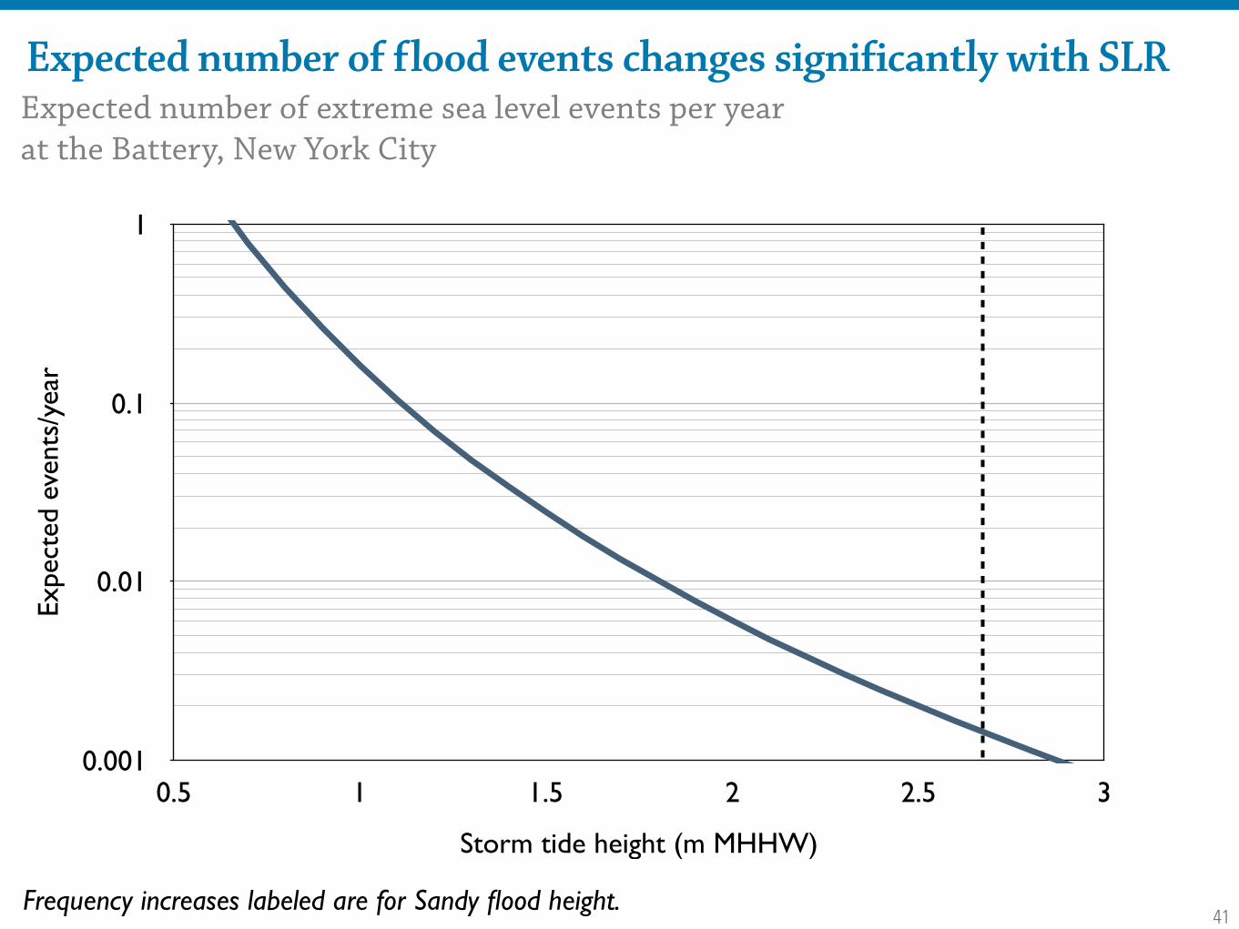
Expected number of flood events changes significantly with SLRExpected number of extreme sea level events per yearat the Battery, New York City
Expe
cted
eve
nts/
year
0.001
0.01
0.1
1
Storm tide height (m MHHW)
0.5 1 1.5 2 2.5 3
Frequency increases labeled are for Sandy flood height.
42
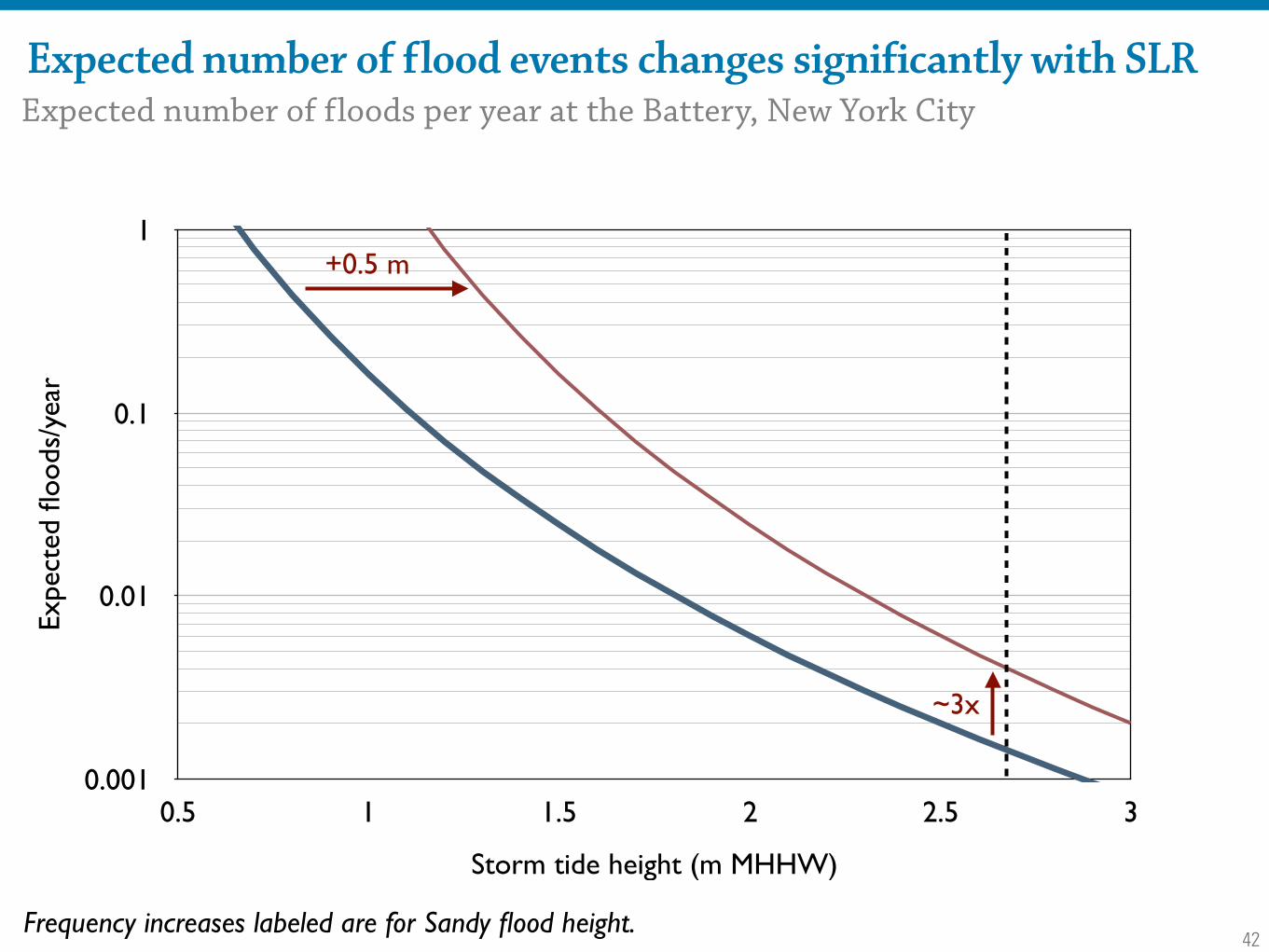
Expected number of flood events changes significantly with SLRExpected number of floods per year at the Battery, New York City
Expe
cted
floo
ds/y
ear
0.001
0.01
0.1
1
Storm tide height (m MHHW)
0.5 1 1.5 2 2.5 3
+0.5 m
~3x
Frequency increases labeled are for Sandy flood height.
43
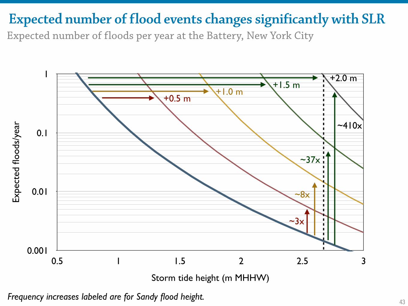
Expected number of flood events changes significantly with SLRExpected number of floods per year at the Battery, New York City
Expe
cted
floo
ds/y
ear
0.001
0.01
0.1
1
Storm tide height (m MHHW)
0.5 1 1.5 2 2.5 3
+0.5 m+1.0 m
+1.5 m+2.0 m
~8x
~37x
~410x
~3x
Frequency increases labeled are for Sandy flood height.

44
It is also necessary to consider the potential effect of changes in surge-driving processes in response to climate change.Expected number of tropical cyclone-driven surges per yearat the Battery, New York City
Garner et al., 2017

45
…and these changes may be correlated with changes in dynamic sea level.
Little et al. (2015)
NATURE CLIMATE CHANGE DOI: 10.1038/NCLIMATE2801 ARTICLESa
4.04.0
3.8
3.6
3.4
3.2
3.0
2.8
2.6
2.4
2.2
2.0
40
Latit
ude
(° N
)
32
24
100 90 80Longitude (° W)
3.6
3.2
2.8
2.4
2.0
1.6
1.2
0.8
0.4
0.0
0.8
0.8
b
Key West
AtlanticCity
Charleston
PensacolaGalveston
Figure 1 | Regions of analysis and CMIP5 RCP 8.5 ensemble SST warming projections. a, Shading indicates the ensemble mean SST change(2080–2099 mean � 1986–2005 mean); contours indicate the ensemble standard deviation. Blue boxes highlight the regions used in the statistical modelof PDI (ref. 29). The solid black box highlights the region included in this analysis. This region is shown in detail in b along with the location of the sites usedto develop the FI.
1
2 3
4 5 6 7
8
9
10
11
12
1314
15
0.0 0.2 0.4 0.6−2
0
2
4
6
8
10
1 2
3 4 5 6 7 8
9
10
11
12
13
1415
0.0 0.2 0.4 0.6−2
0
2
4
6
8
10
5-site mean SLR (m)
RCP 8.5RCP 2.6
1 MRI-CGCM32 CANESM23 CNRM-CM5 4 IPSL-CM5A-MR 5 IPSL-CM5A-LR 6 CCSM4 7 CSIRO-Mk3.6
8 GFDL-ESM2G 9 NorESM1-M 10 HadGEM2-ES11 GFDL-ESM2M 12 MPI-ESM-LR 13 MIROC-ESM14 MIROC-ESM-CHEM15 GFDL-CM3
5-site mean SLR (m)
a b
PDI a
nom
aly
(×10
11 m
3 s−2
)
PDI a
nom
aly
(×10
11 m
3 s−2
)
Figure 2 | CMIP5 ensemble spread in PDI and SLR. Individual AOGCM projections (2080–2099 mean � 1986–2005 mean) of PDI anomaly (y-axis) andmean SLR across the five sites (x-axis) for RCP 2.6 (a) and RCP 8.5 (b). AOGCMs, indicated by numbers, are overlaid on a kernel density estimate of thebivariate probability distribution; shading indicates the normalized probability from 0.9 (darkest) to 0 (white). Red numbers in b are AOGCMs fromgroup 1; blue numbers are group 2 AOGCMs; black numbers show all other AOGCMs (group 3). Dashed lines indicate ensemble mean values.
expansion and also fuel TCs, potentially implying a strong physicallinkage between sea-level changes and TC-driven surges7,13,32. Therelationship between these quantities within and across models hasnot been established.
In this paper, we investigate: changes in PDI and oceanographicSLR (from here forward, denoted as SLR) at five US EastCoast and Gulf Coast locations (Fig. 1b) across a 15-memberAOGCM ensemble; and the joint influence of these two factorson coastal flood risk. Changes in PDI are estimated with thestatistical formulation of Villarini andVecchi33, based on sea surfacetemperature in the tropical North Atlantic relative to the tropicalmean (‘relative SST’; see blue boxes in Fig. 1a for the regionsconsidered). Although this proxy measurement does not captureall large-scale controls on TCs (refs 1,23,24,34,35) or feedbacksbetween TCs, ocean heat content and SLR (refs 36,37), it has beenshown to provide skilful hindcasts and forecasts of North Atlantic
TC activity and intensity33,38,39. Furthermore, this proxy allows theincorporation of a large ensemble of climatemodels, which is criticalgiven the spread in TC-relevant large-scale climate variables shownin other studies1,2,7,25–27.
Sea-level/power dissipation index linkagesFirst, we present the ensemble spread in PDI anomaly and site-averaged SLR over the 2080–2099 period (Fig. 2). In RCP 2.6, whichrequires drastic emission reductions over the twenty-first century,the 15-member ensemble mean projections are 0.21m SLR (five-site average) and 1.1 ⇥ 1011 m3 s�2 PDI anomaly (representing anabsolute PDI > 75% higher than the 1986–2005 mean). Even underrelatively weak forcing, these values exceed the mean rate of SLRand the range of 20-year-mean PDI experienced in the twentiethcentury29,40. Most ensemble members are relatively tightly clusteredaround these values. However, the GFDL-CM3, MIROC-ESM and
NATURE CLIMATE CHANGE | VOL 5 | DECEMBER 2015 | www.nature.com/natureclimatechange 1115
© 2015 Macmillan Publishers Limited. All rights reserved
46
Generalizable lessons
• Instrumental and geological data are crucial for contextualizing and calibrating projections of future changes.
• Probabilistic methods provide a useful way of structuring knowledge, and lend themselves readily to addressing questions about the value of information.
• Interactions among hazards need attention – looking at individual hazards in isolation provides an incomplete picture.
47
Risk assessmentWhat would the consequences be?
48
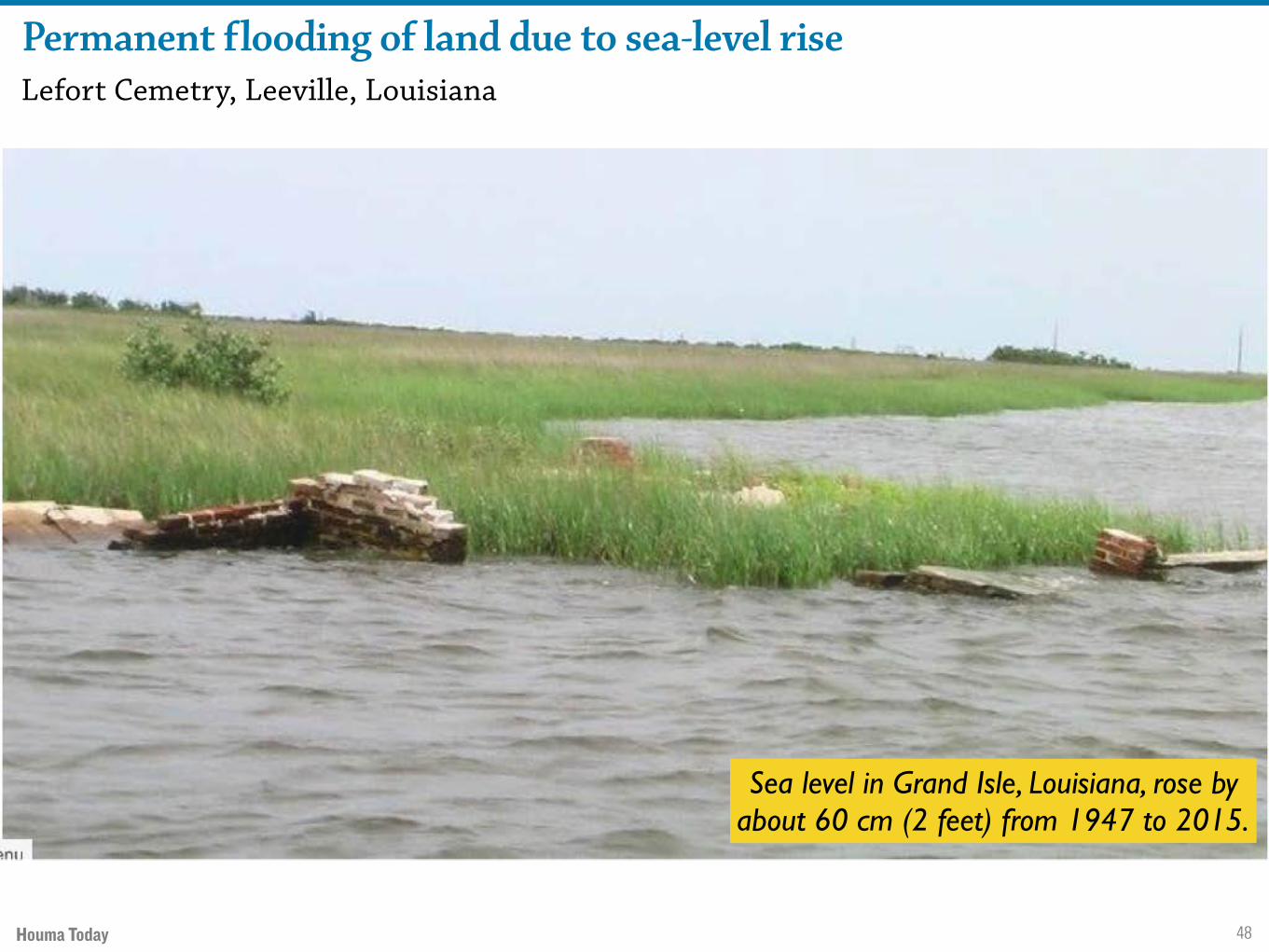
Permanent flooding of land due to sea-level riseLefort Cemetry, Leeville, Louisiana
Houma Today
Sea level in Grand Isle, Louisiana, rose by about 60 cm (2 feet) from 1947 to 2015.
49
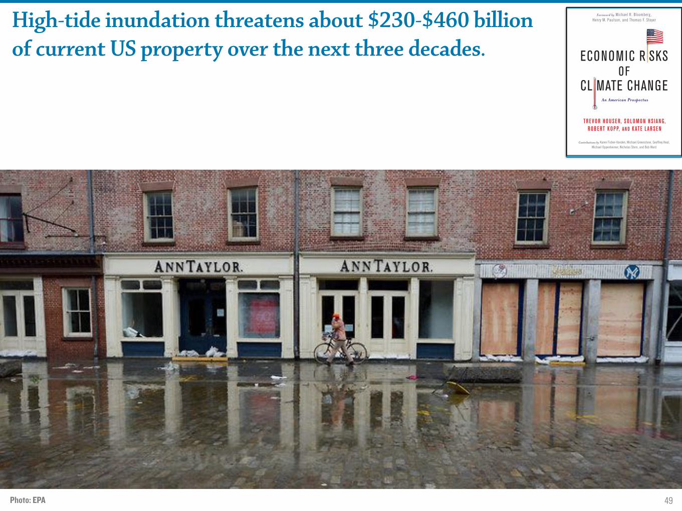
High-tide inundation threatens about $230-$460 billion of current US property over the next three decades.
Photo: EPA
ECONOMIC R SKS OF
CL MATE CHANG EAn American Prospectus
Foreword by Michael R. Bloomberg, Henry M. Paulson, and Thomas F. Steyer
TR E V O R H O US E R , S O LO M O N H S I A N G , R O B E RT KO P P, A N D K ATE L A R S E N
Contributions by Karen Fisher-Vanden, Michael Greenstone, Geoffrey Heal, Michael Oppenheimer, Nicholas Stern, and Bob Ward

50
Storm floodingShip Bottom, NJ
NN2008
(Courtesy Prof. Ken Miller) October 31, 2012
Global sea-level rise from 1880–2012 exposed about 80 thousand additional
people in New York City and New Jersey to Sandy’s storm surge (Miller et al., 2013).
51
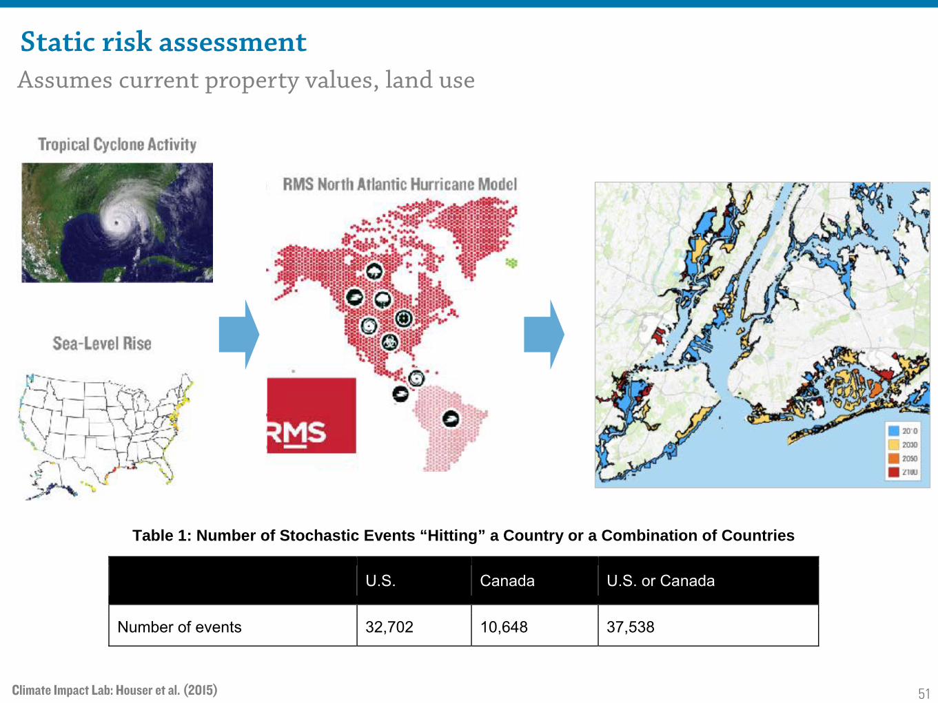
Static risk assessmentAssumes current property values, land use
citationClimate Impact Lab: Houser et al. (2015)
C-5
RMS NORTH ATLANTIC HURRICANE MODEL
Hurricane Modeling
Stochastic Module
The stochastic module consists of a set of thousands of stochastic events that represent more than 100,000 years of hurricane activity. RMS scientists have used state-of-the-art modeling technologies to develop a stochastic event set made of events that are physically realistic and span the range of all possible storms that could occur in the coming years.
At the heart of the stochastic module is a statistical track model that relies on advanced statistical techniques (Hall & Jewson 2007) to extrapolate the HURDAT catalog (Jarvinen et al., 1984) and generate a set of stochastic tracks having similar statistical characteristics to the HURDAT historical tracks. Stochastic tracks are simulated from genesis (starting point) to lysis (last point) using a semi-parametric statistical track model that is based on historical data. Simulated hurricane tracks provide the key drivers of risk, including landfall intensity, landfall frequency, and landfall correlation.
The last step is a calibration process ensuring that simulated landfall frequencies are in agreement with the historical record. Target landfall rates are computed on a set of linear coastal segments (or RMS gates) by smoothing the historical landfall rates. The RMS smoothing technique uses long coastal segments, obtained by extending each RMS gate in both directions and keeping the orientation constant. Historical storms that cross an extended gate contribute to the landfall rate at the corresponding original segment.
Importance sampling of the simulated tracks is performed to create the computationally efficient event set used for loss cost determinations. Some statistics related to the resulting stochastic event set are presented in Table 1.
Table 1: Number of Stochastic Events “Hitting” a Country or a Combination of Countries
U.S. Canada U.S. or Canada
Number of events 32,702 10,648 37,538
Each of these events has a frequency of occurrence given by its mean Poisson rate. Because event frequencies were calibrated against history (HURDAT 1900–2011), this set of Poisson rates represents the RMS baseline model and this rate set is called the “RMS historical rate set.”
Windfield (or Wind Hazard) Module
The wind hazard module calculates windfields from both landfalling hurricanes and bypassing storms. Once tracks and intensities have been simulated by the stochastic module, the windfield module simulates 10 meter, three-second gusts on a variable resolution grid. Size and shape of the time stepping windfields are generated using an analytical wind profile derived from Willoughby (2006). Peak gusts are the driver of building damage and are used as the basis of many building codes world-wide, including the U.S.
Wind Vulnerability Module
The RMS U.S. and Canada Hurricane Models wind vulnerability module relates the expected amount of physical damage to buildings and contents at a location to the modeled peak three-second gust wind speed at that location. The severity of the damage is expressed in terms of a mean damage ratio (MDR), which is defined as the ratio of the expected cost to repair the damaged property to its replacement cost. The wind vulnerability module also estimates the variability in the damage ratio and models it with a beta distribution. Time-element losses due to business interruption and additional living expenses are estimated using occupancy-dependent facility restoration functions that relate the expected duration of the loss of use to the modeled building damage.
Storm Surge Model
The RMS North Atlantic Hurricane Model storm surge system utilizes the latest technology and storm surge hazard assessment methodologies to quantify the risk of storm surge for the U.S. Atlantic and Gulf coastlines (from Texas to Maine), as well as for parts of the Caribbean. The model system uses wind and pressure fields from the stochastic event set of the RMS North Atlantic Hurricane Model as forcing (i.e., as input) for the state-of-the-art MIKE 21 hydrodynamic model system to estimate still-water (i.e. without wave effects) storm surge. This hydrodynamic model system is also used to determine wave heights and resulting hazard statistics for offshore platforms. The impact of rainfall accumulation during an event is not considered in the modeling of storm surge levels.
52
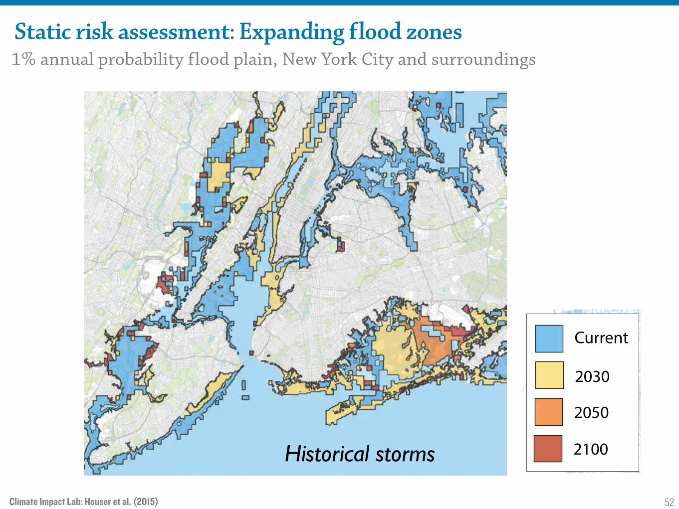
Static risk assessment: Expanding flood zones1% annual probability flood plain, New York City and surroundings
A
B F
C ECurrent
2030
2100
2050
C
D
0.0
0.1
0.2
0.3
0.4
0.5
0.6
0.7
0.8
0.9
2010 2020 2030 2040 2050 2060 2070 2080 2090 2100
0.2%
0.1%
0.5%
0.9%
1.8%
0.3%
0.4%
1.1%
1.5%
3.1%
0.4%
0.7%
1.5%
1.6%
4.1%
0.4%
0.8%
1.7%
1.7%
4.5%
0
1
2
3
4
5
Dam
ages
(% o
f Gro
ss S
tate
Pro
duct
)
Current Storm Activity
Plus Median MSL rise
Plus 1-in-20 MSL rise
Plus 1-in-100 MSL rise
Dam
ages
(% o
f Gro
ss D
omes
tic P
rodu
ct)
Texas New York S. Carolina Louisiana Florida
Projected Storm Activity, median MSL rise(median, 90% CI)
Historical Storm Activity, median MSL rise(median, 90% CI)Historical Storm Activity, historical sea level
Figure 4: Sea level rise and coastal damage from tropical cyclones. (A) Example 100-year floodplain in Miami, FL under median sealevel rise for RCP 8.5, assuming no change in tropical cyclone activity. (B) Same, but accounting for projected changes in tropical cycloneactivity. (C) Same as (A) but for New York, NY. (D) Same as (B) but for New York, NY. (E) Annual average direct property damagesfrom tropical cyclones in five most a↵ected states, assuming installed infrastructure and tropical cyclone activity is held fixed at current levels.Bars indicate capital losses under current sea level, median, 95th-percentile and 99.5th-percentile sea level rise in RCP 8.5 in 2100. (F) Annualaverage direct property damages nationally aggregated in RCP 8.5 assuming historical and projected tropical cyclone activity, assuming installedinfrastructure is held fixed at current levels and median sea level rise. Historical storm damage is dashed line.
12
Historical storms
Climate Impact Lab: Houser et al. (2015)

53
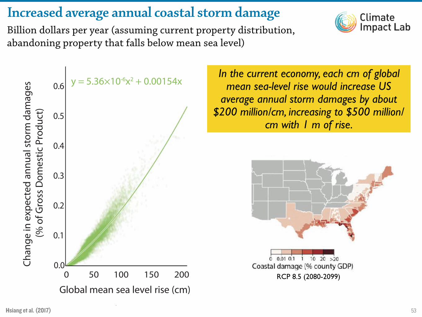
Increased average annual coastal storm damageBillion dollars per year (assuming current property distribution, abandoning property that falls below mean sea level)
Hsiang et al. (2017)
form suggests losses of ∼1.2% GDP per 1°C onaverage in our sample of scenarios (table S16).The greatest direct cost forGMST changes larger
than 2.5°C is the burden of excessmortality, withsizable but smaller contributions from changesin labor supply, energy demand, and agriculturalproduction (Fig. 5B). Coastal storm impacts arealso sizable but do not scale strongly with GMSTbecause projections of globalMSL are dependenton RCP but are not explicitly calculated as func-tions of GMST (36), causing the coastal stormcontribution to the slope of the damage functionto be relatively muted. It is possible to use alter-native approaches to valuing mortality in whichthe loss of lives for older and/or low-income indi-viduals are assigned lower value than those ofyounger and/or high-income individuals (44), anadjustment that would alter damages differentlyfor different levels of warming based on the ageand income profile of affected individuals (e.g.,fig. S13). Here, we focus on the approach legallyadoptedby theU.S. government for environmentalcost-benefit analysis, in which the lives of all indi-viduals are valued equally (37). Because the VSLparameter is influential, challenging to measure
empirically, and may evolve in the future, its in-fluence on damages is an important area for fu-ture investigation.
Risk and inequality of totallocal damages
Climate change increases the unpredictability andbetween-county inequality of future economic out-comes, effects that may alter the valuation of cli-mate damages beyond their nationally averagedexpected costs (45). Figure 5C displays the prob-ability distribution of damage under RCP8.5 as afraction of county income, ordering counties bytheir current income per capita. Median damagesare systematically larger in low-income counties,increasing by 0.93% of county income (95% confi-dence interval = 0.85 to 1.01%) on average foreach reduction in current income decile. In therichest third of counties, the average very likelyrange (90% credible interval, determined as theaverage of 5th and 95th percentile values acrosscounties) for damages is −1.2 to 6.8% of countyincome (negative damages are benefits), whereasfor the poorest third of counties, the averagerange is 2.0 to 19.6% of county income. These
differences are more extreme for the richest 5%and poorest 5% of counties, with average inter-vals for damage of −1.1 to 4.2% and 5.5 to 27.8%,respectively.We note that it is possible to adjust the aggre-
gate damage function in Fig. 5A to capture socie-tal aversion to both the risk and inequality in Fig.5C. In SMsectionK,wedemonstrate one approachto constructing such inequality-neutral, certainty-equivalent damage functions. Depending on theparameters used to value risk and inequality,accounting for these factors may dramaticallyinfluence society’s valuation of damages in aman-ner similar to the large influence of discount rateson the valuation of future damages (46). This find-ing highlights risk and inequality valuation as cri-tical areas for future research.
Discussion
Our results provide a probabilistic, national dam-age function based on spatially disaggregated,empirical, longitudinal analyses of climate im-pacts and available global climate models, butit will not be the last estimate. Because we usestringent selection criteria for empirical studies,
Hsiang et al., Science 356, 1362–1369 (2017) 30 June 2017 5 of 7
Fig. 4. Economic costs of sea level rise interacting with cyclones.(A) Example 100-year floodplain in Miami, Florida, under median sealevel rise for RCP8.5, assuming no change in tropical cyclone activity.(B) Same, but accounting for projected changes in tropical cycloneactivity. (C) Same as (A), but for New York, New York. (D) Same as (B), butfor New York, New York. (E) Annual average direct property damages fromtropical cyclones and extratropical cyclones in the five most-affectedstates, assuming that installed infrastructure and cyclone activity is
held fixed at current levels. Bars indicate capital losses under currentsea level, median, 95th-percentile and 99th-percentile sea level rise inRCP8.5 in 2100. (F) Nationally aggregated additional annual damagesabove historical versus global mean sea level rise holding stormfrequency fixed. (G) Annual average direct property damages nationallyaggregated in RCP8.5, incorporating mean sea level rise and eitherhistorical or projected tropical cyclone activity. Historical stormdamage is the dashed line.
RESEARCH | RESEARCH ARTICLE
on June 29, 2017
http://science.sciencemag.org/
Dow
nloaded from
RCP 8.5 (2080-2099)
53
Increased average annual coastal storm damageBillion dollars per year (assuming current property distribution, abandoning property that falls below mean sea level)
Hsiang et al. (2017)
form suggests losses of ∼1.2% GDP per 1°C onaverage in our sample of scenarios (table S16).The greatest direct cost forGMST changes larger
than 2.5°C is the burden of excessmortality, withsizable but smaller contributions from changesin labor supply, energy demand, and agriculturalproduction (Fig. 5B). Coastal storm impacts arealso sizable but do not scale strongly with GMSTbecause projections of globalMSL are dependenton RCP but are not explicitly calculated as func-tions of GMST (36), causing the coastal stormcontribution to the slope of the damage functionto be relatively muted. It is possible to use alter-native approaches to valuing mortality in whichthe loss of lives for older and/or low-income indi-viduals are assigned lower value than those ofyounger and/or high-income individuals (44), anadjustment that would alter damages differentlyfor different levels of warming based on the ageand income profile of affected individuals (e.g.,fig. S13). Here, we focus on the approach legallyadoptedby theU.S. government for environmentalcost-benefit analysis, in which the lives of all indi-viduals are valued equally (37). Because the VSLparameter is influential, challenging to measure
empirically, and may evolve in the future, its in-fluence on damages is an important area for fu-ture investigation.
Risk and inequality of totallocal damages
Climate change increases the unpredictability andbetween-county inequality of future economic out-comes, effects that may alter the valuation of cli-mate damages beyond their nationally averagedexpected costs (45). Figure 5C displays the prob-ability distribution of damage under RCP8.5 as afraction of county income, ordering counties bytheir current income per capita. Median damagesare systematically larger in low-income counties,increasing by 0.93% of county income (95% confi-dence interval = 0.85 to 1.01%) on average foreach reduction in current income decile. In therichest third of counties, the average very likelyrange (90% credible interval, determined as theaverage of 5th and 95th percentile values acrosscounties) for damages is −1.2 to 6.8% of countyincome (negative damages are benefits), whereasfor the poorest third of counties, the averagerange is 2.0 to 19.6% of county income. These
differences are more extreme for the richest 5%and poorest 5% of counties, with average inter-vals for damage of −1.1 to 4.2% and 5.5 to 27.8%,respectively.We note that it is possible to adjust the aggre-
gate damage function in Fig. 5A to capture socie-tal aversion to both the risk and inequality in Fig.5C. In SMsectionK,wedemonstrate one approachto constructing such inequality-neutral, certainty-equivalent damage functions. Depending on theparameters used to value risk and inequality,accounting for these factors may dramaticallyinfluence society’s valuation of damages in aman-ner similar to the large influence of discount rateson the valuation of future damages (46). This find-ing highlights risk and inequality valuation as cri-tical areas for future research.
Discussion
Our results provide a probabilistic, national dam-age function based on spatially disaggregated,empirical, longitudinal analyses of climate im-pacts and available global climate models, butit will not be the last estimate. Because we usestringent selection criteria for empirical studies,
Hsiang et al., Science 356, 1362–1369 (2017) 30 June 2017 5 of 7
Fig. 4. Economic costs of sea level rise interacting with cyclones.(A) Example 100-year floodplain in Miami, Florida, under median sealevel rise for RCP8.5, assuming no change in tropical cyclone activity.(B) Same, but accounting for projected changes in tropical cycloneactivity. (C) Same as (A), but for New York, New York. (D) Same as (B), butfor New York, New York. (E) Annual average direct property damages fromtropical cyclones and extratropical cyclones in the five most-affectedstates, assuming that installed infrastructure and cyclone activity is
held fixed at current levels. Bars indicate capital losses under currentsea level, median, 95th-percentile and 99th-percentile sea level rise inRCP8.5 in 2100. (F) Nationally aggregated additional annual damagesabove historical versus global mean sea level rise holding stormfrequency fixed. (G) Annual average direct property damages nationallyaggregated in RCP8.5, incorporating mean sea level rise and eitherhistorical or projected tropical cyclone activity. Historical stormdamage is the dashed line.
RESEARCH | RESEARCH ARTICLE
on June 29, 2017
http://science.sciencemag.org/
Dow
nloaded from
RCP 8.5 (2080-2099)
In the current economy, each cm of global mean sea-level rise would increase US
average annual storm damages by about $200 million/cm, increasing to $500 million/
cm with 1 m of rise.
53
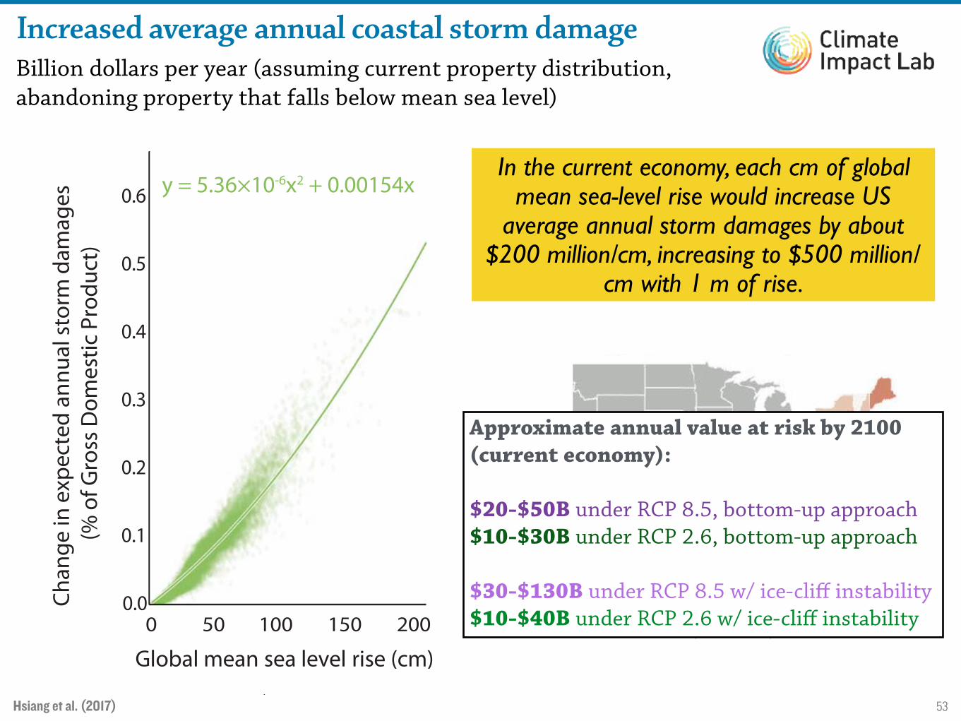
Increased average annual coastal storm damageBillion dollars per year (assuming current property distribution, abandoning property that falls below mean sea level)
Hsiang et al. (2017)
form suggests losses of ∼1.2% GDP per 1°C onaverage in our sample of scenarios (table S16).The greatest direct cost forGMST changes larger
than 2.5°C is the burden of excessmortality, withsizable but smaller contributions from changesin labor supply, energy demand, and agriculturalproduction (Fig. 5B). Coastal storm impacts arealso sizable but do not scale strongly with GMSTbecause projections of globalMSL are dependenton RCP but are not explicitly calculated as func-tions of GMST (36), causing the coastal stormcontribution to the slope of the damage functionto be relatively muted. It is possible to use alter-native approaches to valuing mortality in whichthe loss of lives for older and/or low-income indi-viduals are assigned lower value than those ofyounger and/or high-income individuals (44), anadjustment that would alter damages differentlyfor different levels of warming based on the ageand income profile of affected individuals (e.g.,fig. S13). Here, we focus on the approach legallyadoptedby theU.S. government for environmentalcost-benefit analysis, in which the lives of all indi-viduals are valued equally (37). Because the VSLparameter is influential, challenging to measure
empirically, and may evolve in the future, its in-fluence on damages is an important area for fu-ture investigation.
Risk and inequality of totallocal damages
Climate change increases the unpredictability andbetween-county inequality of future economic out-comes, effects that may alter the valuation of cli-mate damages beyond their nationally averagedexpected costs (45). Figure 5C displays the prob-ability distribution of damage under RCP8.5 as afraction of county income, ordering counties bytheir current income per capita. Median damagesare systematically larger in low-income counties,increasing by 0.93% of county income (95% confi-dence interval = 0.85 to 1.01%) on average foreach reduction in current income decile. In therichest third of counties, the average very likelyrange (90% credible interval, determined as theaverage of 5th and 95th percentile values acrosscounties) for damages is −1.2 to 6.8% of countyincome (negative damages are benefits), whereasfor the poorest third of counties, the averagerange is 2.0 to 19.6% of county income. These
differences are more extreme for the richest 5%and poorest 5% of counties, with average inter-vals for damage of −1.1 to 4.2% and 5.5 to 27.8%,respectively.We note that it is possible to adjust the aggre-
gate damage function in Fig. 5A to capture socie-tal aversion to both the risk and inequality in Fig.5C. In SMsectionK,wedemonstrate one approachto constructing such inequality-neutral, certainty-equivalent damage functions. Depending on theparameters used to value risk and inequality,accounting for these factors may dramaticallyinfluence society’s valuation of damages in aman-ner similar to the large influence of discount rateson the valuation of future damages (46). This find-ing highlights risk and inequality valuation as cri-tical areas for future research.
Discussion
Our results provide a probabilistic, national dam-age function based on spatially disaggregated,empirical, longitudinal analyses of climate im-pacts and available global climate models, butit will not be the last estimate. Because we usestringent selection criteria for empirical studies,
Hsiang et al., Science 356, 1362–1369 (2017) 30 June 2017 5 of 7
Fig. 4. Economic costs of sea level rise interacting with cyclones.(A) Example 100-year floodplain in Miami, Florida, under median sealevel rise for RCP8.5, assuming no change in tropical cyclone activity.(B) Same, but accounting for projected changes in tropical cycloneactivity. (C) Same as (A), but for New York, New York. (D) Same as (B), butfor New York, New York. (E) Annual average direct property damages fromtropical cyclones and extratropical cyclones in the five most-affectedstates, assuming that installed infrastructure and cyclone activity is
held fixed at current levels. Bars indicate capital losses under currentsea level, median, 95th-percentile and 99th-percentile sea level rise inRCP8.5 in 2100. (F) Nationally aggregated additional annual damagesabove historical versus global mean sea level rise holding stormfrequency fixed. (G) Annual average direct property damages nationallyaggregated in RCP8.5, incorporating mean sea level rise and eitherhistorical or projected tropical cyclone activity. Historical stormdamage is the dashed line.
RESEARCH | RESEARCH ARTICLE
on June 29, 2017
http://science.sciencemag.org/
Dow
nloaded from
RCP 8.5 (2080-2099)
In the current economy, each cm of global mean sea-level rise would increase US
average annual storm damages by about $200 million/cm, increasing to $500 million/
cm with 1 m of rise.
Approximate annual value at risk by 2100 (current economy):
$20-$50B under RCP 8.5, bottom-up approach $10-$30B under RCP 2.6, bottom-up approach
$30-$130B under RCP 8.5 w/ ice-cliff instability $10-$40B under RCP 2.6 w/ ice-cliff instability

54
While our analysis methods often focus on impacts in isolation, they interact at both physical (e.g., rain + coastal flooding) and economic levels.
Thus it is important to develop integrated frameworks that can look at the interactions among hazards and risks.
Hsiang et al. (2017)
to reduce yields ∼12.1 (±0.7) % per °C (see alsofigs. S11 and S12 and tables S10 and S11).Rising mortality in hot locations more than
offsets reductions in cool regions, so annual na-tional mortality rates rise ∼5.4 (±0.5) deaths per100,000 per °C (Fig. 3C). For lower GMST changes,this is driven by mortality between ages 1 and 44and by infant mortality and ages ≥45 for largerGMST increases (fig. S13 and table S12).Electricity demand rises on net for all GMST
changes, roughly 5.3 (± 0.14) % per °C, becauserising demand from hot days more than offsetsfalling demand on cool days (Fig. 3D and tableS13). Because total costs in the energy sector arecomputed using NEMS, demand is not statistical-ly resampled as other sectors are (SM section G).Total hours of labor supplied declines ∼0.11
(±0.004) % per °C in GMST for low-risk workers,who are predominantly not exposed to outdoortemperatures, and 0.53 (±0.01) % per °C for high-risk workers who are exposed (∼23% of all em-ployed workers, in sectors such as construction,
mining, agriculture, and manufacturing) (Fig. 3,E and F, and table S14).Property crime increases as the number of cold
days—which suppress property crime rates (fig.S4)—falls but then flattens for higher levels ofwarming because hot days do not affect propertycrime rates. Violent crime rates increase linearlyat a relatively precise 0.88 (±0.04) % per °C inGMST (Fig. 3, G and H, and table S15).Coastal impacts are driven by the amplifica-
tion of tropical cyclone and extratropical cyclonestorm tides by local MSL rise and by the alter-ation of the frequency, distribution, and intensityof these cyclones (SM section H). Rising MSLincreases the storm tide height and floodplainduring cyclones: Fig. 4, A to D, illustrates how 1-in-100-year floodplains evolve over time due toMSL rise (RCP8.5) with and without projectedchanges in cyclones for two major coastal cities.Coastal impacts are distributed highly unequally,with acute impacts for eastern coastal states withtopographically low cities; MSL rise alone raises
expected direct annual economic damage 0.6to 1.3% of state gross domestic product (GDP) forSouth Carolina, Louisiana, and Florida in themedian case, and 0.7 to 2.3% for the 95th per-centile of MSL rise (Fig. 4E) (RCP8.5). Nation-ally, MSL rise would increase annual expectedstorm damages roughly 0.0014% GDP per cm ifcapital and storm frequency remain fixed (Fig.4F). Accounting for the projected alteration ofthe TC distribution roughly doubles the damagefrom MSL rise, the two combined costing an es-timated additional 0.5 (±0.2) % of GDP annuallyin 2100 when aggregated nationally (Fig. 4G).
Uncertainty
At the county level, conditional upon RCP, un-certainty in direct damages is driven by climateuncertainty (both in GMST and in the expectedspatiotemporal distribution of changes conditionalon GMST), by within-month weather exposure,and by statistical assumptions and sampling usedto derive dose-response functions, as well as by
Hsiang et al., Science 356, 1362–1369 (2017) 30 June 2017 3 of 7
Fig. 2. Spatial distributions of projected damages. County-level medianvalues for average 2080 to 2099 RCP8.5 impacts. Impacts are changesrelative to counterfactual “no additional climate change” trajectories.Color indicates magnitude of impact in median projection; outline colorindicates level of agreement across projections (thin white outline, inner66% of projections disagree in sign; no outline, ≥83% of projections agreein sign; black outline, ≥95% agree in sign; thick white outline, stateborders; maps without outlines shown in fig. S2). Negative damagesindicate economic gains. (A) Percent change in yields, area-weighted
average for maize, wheat, soybeans, and cotton. (B) Change in all-causemortality rates, across all age groups. (C) Change in electricity demand.(D) Change in labor supply of full-time-equivalent workers for low-riskjobs where workers are minimally exposed to outdoor temperature.(E) Same as (D), except for high-risk jobs where workers are heavilyexposed to outdoor temperatures. (F) Change in damages fromcoastal storms. (G) Change in property-crime rates. (H) Changein violent-crime rates. (I) Median total direct economic damage acrossall sectors [(A) to (H)].
RESEARCH | RESEARCH ARTICLE
on June 29, 2017
http://science.sciencemag.org/
Dow
nloaded from

55
Impacts can have surprising systemic effectsPercentage loss in total cell real GDP in 2200 (RCP 4.5)
Desmet, Kopp, Nagy, Oppenheimer and Rossi-Hansberg. (in rev.)
Fig. 3. (a) Percentage mean loss in total cell real GDP in 2200 under RCP 4.5. (b) Percentage mean population change by cell in 2200 under RCP 4.5.
Percentage Loss in Total Cell Real GDP in 2200 (RCP 4.5) (nonflooding scenario / mean of flooding scenarios)-1
!
!
Percentage Loss in Total Cell Population in 2200 (RCP 4.5) (nonflooding scenario / mean of flooding scenarios)-1
!
!
Fig. 4. Cumulative density functions of (a) the PDV of total percentage losses in real GDP, and (b) the population losses for coastal and inland cells in2200 (RCP 4.5).
10%9%8%7%6%5%4%3%2%1%0%-1%Percentage Real GDP Loss
0
0.1
0.2
0.3
0.4
0.5
0.6
0.7
0.8
0.9
1
CD
F
CDF of Mean PDV Losses in Real GDP
Coastal CellsInland Cells
-2% 0% 2% 4% 6% 8% 10% 12% 14% 16% 18% 20%Percentage Population Loss
0
0.1
0.2
0.3
0.4
0.5
0.6
0.7
0.8
0.9
1C
DF
CDF of Mean Population Losses in 2200
Coastal Cells
Inland Cells
Given the complexity of the issue at hand, our model necessarilyleaves out some important aspects. First, although we accountfor the uncertainty in flooding scenarios, and we demonstrate therobustness of our evaluation to a variety of economic parameters,our evaluation does not include potential measurement error ineconomic variables or model misspecification. Second, we donot account for feedback loops between economic outcomes andflooding through changed emissions pathways. Third, we onlyanalyze the impact of permanent, albeit gradual, inundation andnot temporary flooding caused by extreme weather events. Finally,we do not model efforts to mitigate flooding using a variety ofmethods such as barriers and dikes. Future work should focus onextending this research in these directions, to improve further ourestimates of the economic consequences of coastal flooding.
Materials and Methods
Quantification and simulation. We discretize the world into 64,800 1¶ ◊1¶ cells. Structural parameter values are partly taken from the literatureand partly estimated from data. Throughout, we use the parameters ofthe baseline simulation in ref. 20. For the year 2000, we use data on thegeographic distribution of population and output per worker from G-Econ4.0 (27) to invert the model and recover local productivity measures. Wealso need estimates of amenities for all grid cells. In a world with perfectmobility, it is enough to have information on population and productivity toget such estimates: locations with low productivity but large populationsmust have good amenities. However, when mobility is limited, those samelow-productivity, high-density locations might also be low-utility places thatare hard to leave. In a world with restricted mobility, we therefore need dataon utility, as well as population and productivity, to estimate local amenities.To that end, we use country-level survey data on subjective well-being fromthe Gallup World Poll (28).¶ Subjective well-being, measured on a scale
¶Because the data are at the country level, there are no utility differences across locations withincountries in the initial period. Such utility differences do arise in future periods.
6

56
Generalizable Lessons and Research Needs
• Instrumental and geological data are crucial for contextualizing and calibrating projections of future changes.
• Probabilistic methods provide a useful way of structuring knowledge, and lend themselves readily to addressing questions about the value of information.
• Interactions among hazards and risks need attention – looking at individual hazards/risks in isolation provides an incomplete picture.

57
Risk managementWhat might we as a society do about it?

58
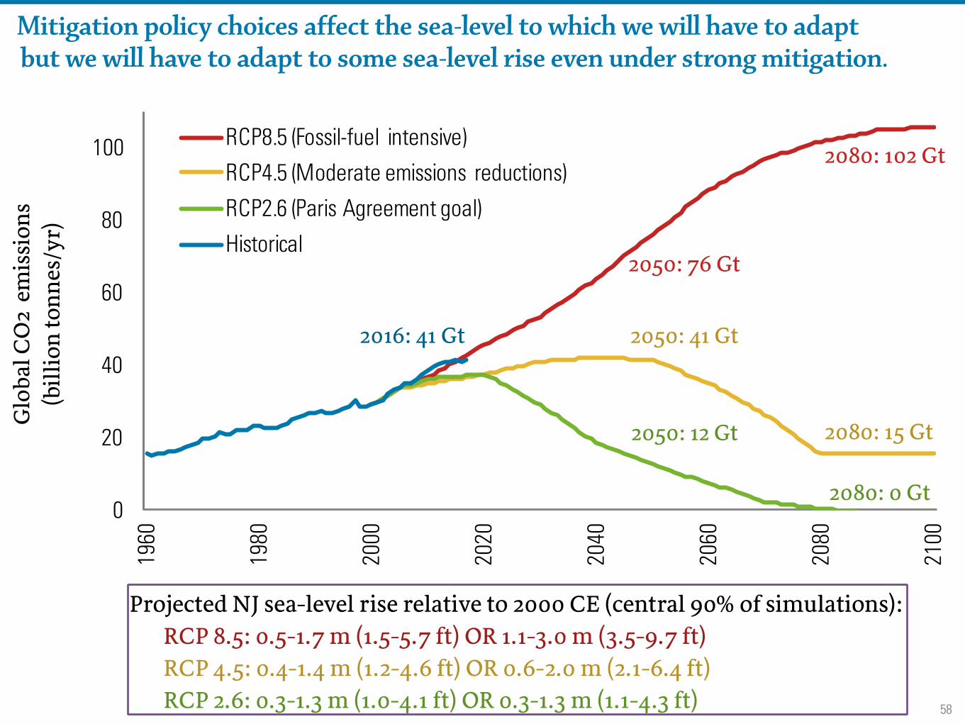
Mitigation policy choices affect the sea-level to which we will have to adapt
Projected NJ sea-level rise relative to 2000 CE (central 90% of simulations): RCP 8.5: 0.5-1.7 m (1.5-5.7 ft) OR 1.1-3.0 m (3.5-9.7 ft) RCP 4.5: 0.4-1.4 m (1.2-4.6 ft) OR 0.6-2.0 m (2.1-6.4 ft) RCP 2.6: 0.3-1.3 m (1.0-4.1 ft) OR 0.3-1.3 m (1.1-4.3 ft)
0
20
40
60
80
1001
96
0
19
80
20
00
20
20
20
40
20
60
20
80
21
00
RCP8.5 (Fossil-fuel intensive)
RCP4.5 (Moderate emissions reductions)
RCP2.6 (Paris Agreement goal)
Historical2050: 76 Gt
2016: 41 Gt 2050: 41 Gt
2050: 12 Gt
2080: 102 Gt
2080: 15 Gt
2080: 0 Gt
Glo
bal C
O2
em
issi
ons
(bill
ion
tonn
es/y
r)
58
Mitigation policy choices affect the sea-level to which we will have to adapt
Projected NJ sea-level rise relative to 2000 CE (central 90% of simulations): RCP 8.5: 0.5-1.7 m (1.5-5.7 ft) OR 1.1-3.0 m (3.5-9.7 ft) RCP 4.5: 0.4-1.4 m (1.2-4.6 ft) OR 0.6-2.0 m (2.1-6.4 ft) RCP 2.6: 0.3-1.3 m (1.0-4.1 ft) OR 0.3-1.3 m (1.1-4.3 ft)
but we will have to adapt to some sea-level rise even under strong mitigation.
0
20
40
60
80
1001
96
0
19
80
20
00
20
20
20
40
20
60
20
80
21
00
RCP8.5 (Fossil-fuel intensive)
RCP4.5 (Moderate emissions reductions)
RCP2.6 (Paris Agreement goal)
Historical2050: 76 Gt
2016: 41 Gt 2050: 41 Gt
2050: 12 Gt
2080: 102 Gt
2080: 15 Gt
2080: 0 Gt
Glo
bal C
O2
em
issi
ons
(bill
ion
tonn
es/y
r)
59
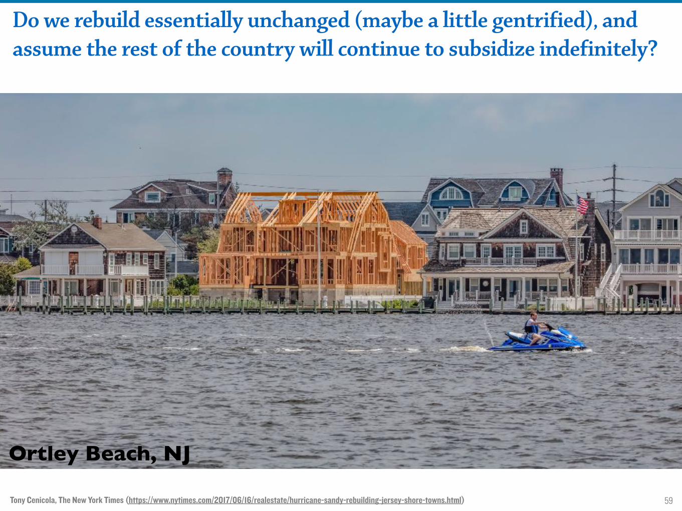
Do we rebuild essentially unchanged (maybe a little gentrified), and assume the rest of the country will continue to subsidize indefinitely?
Tony Cenicola, The New York Times (https://www.nytimes.com/2017/06/16/realestate/hurricane-sandy-rebuilding-jersey-shore-towns.html)
Ortley Beach, NJ
60Tony Cenicola, The New York Times (https://www.nytimes.com/2017/06/16/realestate/hurricane-sandy-rebuilding-jersey-shore-towns.html)
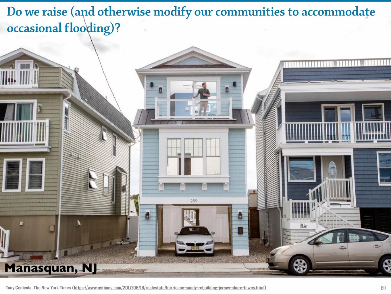
Manasquan, NJ
Do we raise (and otherwise modify our communities to accommodate occasional flooding)?

61
Do we harden?
BIG-Bjarke Ingels Group (2017)
Proposed East Side Coastal Resiliency Project

62
Do we expand protective natural infrastructure?
Photo: Jamaica Bay Ecowatchers
New oyster beds in Jamaica Bay
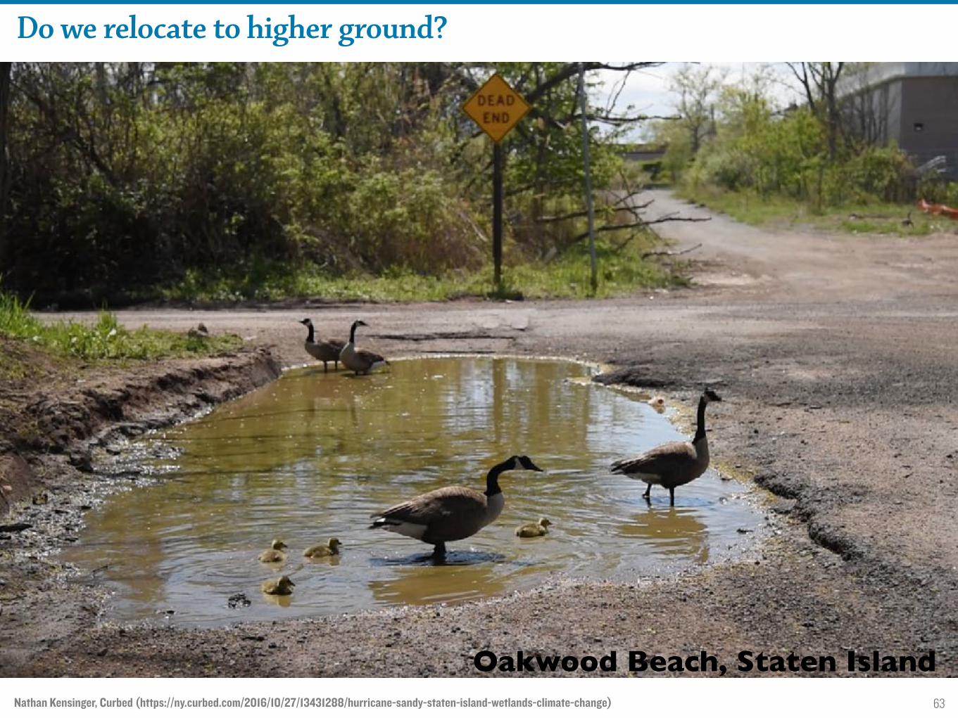
63
Do we relocate to higher ground?
Nathan Kensinger, Curbed (https://ny.curbed.com/2016/10/27/13431288/hurricane-sandy-staten-island-wetlands-climate-change)
Oakwood Beach, Staten Island
64
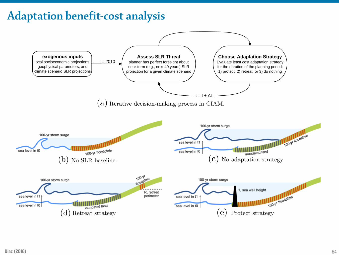
Adaptation benefit-cost analysis
Diaz (2016)
Climatic Change (2016) 137:143–156 147
Fig. 1 Diagrams of CIAM algorithm and adaptation strategies. a Each segment follows an iterative decision-making process, choosing the least-cost adaptation strategy for the current planning period; this processrepeats over the model time horizon. b No SLR. Baseline floodplain for an illustrative 100-year extreme(shown in red); this may drive some initial level of adaptation prior to SLR. c No adaptation. SLR causesincremental loss of inundated land (shown in gray), incurring reactive retreat costs. The new 100-year flood-plain exposes new land depending on the coastal topography. This may be the least-cost strategy in someundeveloped areas. d Retreat. SLR causes the loss of inundated land and incurs planned relocation costsbelow the retreat perimeterR. Expected flood damage is limited to extremes that penetrate the retreat perime-ter (e.g., ≥ R). e Protect. Land is protected from SLR damages by the sea wall with height H . In additionto protection costs, overtopping extremes (e.g., ≥ H ) incur an expected flood cost. The impact of SLR onwetlands is not depicted in the diagram. In the application presented in Section 3, CIAM will evaluate theseadaptation strategies for several SLR scenarios
where ∆t is the decision-making planning period of annual time-steps t , r is the discountrate of 4 %, and s is the adaptation strategy (i.e., protect, retreat, or do nothing and the extent,since extra adaptation can be pursued to minimize the expected cost of flood impacts).CIAM makes the simplifying assumption that the near-term extent of local SLR is knownwith perfect foresight for a given climate scenario.6 Adaptation investments are made incre-mentally and modularly, and the chosen strategy is updated over time following an iterativeprocess depicted in Fig. 1.7
These strategies can be summarized diagrammatically. Figure 1b shows the counterfac-tual baseline case of no climate-driven SLR, against which all climate scenarios will becompared. Figures 1c–e show the cases corresponding to the three adaptation strategies: noadaptation, retreat, and protect.
6Although perfect foresight is unrealistic, this simplified construction of SLR ‘learning’ follows from therelatively smooth near-term rise driven by thermal inertia, whereas other climate changes are likely to bemore abrupt or difficult to detect (e.g., thermohaline circulation; Keller et al. 2008).7The adaptation planning period (∆t) is assumed to be 40 years; a 100-year period is considered as asensitivity analysis, given major coastal defense structures may be planned for a longer duration.

65
Adaptation benefit-cost analysis
Diaz et al. (2016)
Climatic Change (2016) 137:143–156 151
No SLR RCP2.6 RCP4.5 RCP8.5
0
1
2
3
0.0
0.1
0.2
0.3
No
Ad
ap
tatio
nL
ea
st−
Co
st
20
10
20
50
21
00
20
10
20
50
21
00
20
10
20
50
21
00
20
10
20
50
21
00
an
nu
al co
st
($T
)
Cost Typeflood
wetland
inundation
retreat
protection
Fig. 2 Annual damage and adaptation costs for the No Adaptation (top) and the Least-Cost policies (bottom,note y-axis scale change) for the no SLR baseline and three RCP scenarios (column). Error bars show the5th–95th percentile range for global SLR scenario. No Adaptation assumes segments do nothing in advanceof SLR, with permanent loss of inundated land and capital and reactive retreat. Least-Cost shows costs wheneach local segment pursues its own optimal strategy, updating the adaptation decision every 40–50 years
global GDP projection, respectively). On a per-county basis the median cost of adaptationin 2050 is estimated to be under 0.09 % of national GDP, although certain countries willbe impacted disproportionately—the four countries with the largest burden are the MarshallIslands (7.6 %), the Maldives (7.5 %), Tuvalu (4.6 %), and Kiribati (4.1 %). On an absolutebasis, the four countries facing the largest net present value (NPV) of costs from 2010 to2100 are the United States ($419 billion), Australia ($208 billion), Brazil ($98 billion), andChina ($87 billion). Cost results in terms of NPV and as a percentage of national GDP,decomposed into protection, retreat, expected flood cost, and residual costs are reported inTable SM1 for the top 15 countries, with complete results for all countries in Table SM2.It is worth noting that while flood damages are modeled (and reported) in expectation, therealized cost of any one stochastic event could constitute a more substantial fraction of acountry’s GDP.
3.3 CIAM results: local coastal adaptation maps
CIAM’s underlying spatial resolution is displayed in Fig. 3 with maps showing each of the12,148 coastal segments and the adaptation strategy pursued in 2050.
This figure illustrates that retreat is cost-effective for the majority of the world’s coast-lines, while protection is pursued selectively in areas that are very dense in people andcapital and have extensive low-lying areas exposed to both inundation and flooding. Forboth protect and retreat it is often optimal for coastal segments to pursue additional adapta-tion above what is strictly required by rising seas in order to lessen the impact of uncertainflooding on an annual basis. These geographical results highlight a defining feature ofCIAM, the fact that adaptation decisions and costs are evaluated at the local level, where itwill ultimately take place.
66
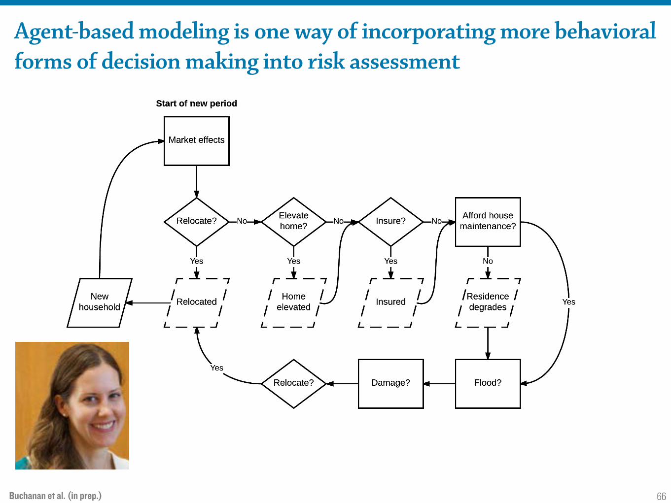
Agent-based modeling is one way of incorporating more behavioral forms of decision making into risk assessment
Buchanan et al. (in prep.)
The Resilience Evaluation Model 5
Fig. 3 Overview of initialization and an annual time step of the model (which is repeated for 30 years). Model processes arerepresented by rectangles, decisions by triangles, and key state variable outcomes by slanted squares. Resilience indicators aredashed.
vp/rp:r, where rp:r is the price-to-rent ratio (µ = 19.4, sd = 1.0 from 2010-2016; Zillow, 2016). Householdincome h is initially set as:
h =
((ct + cm)/⌧ for homeownerscr/⌧ for renters
(1)
where ⌧ is the fraction of income spent on housing, equal to 0.26, the average across Jamaica Bay households.cm are annual mortgage payments, estimated by:
cm =l ⇤ ri
1� (1 + ri)�N(2)
where l is the loan’s principle, ri is the annual interest rate set to 5%, and N is the loan’s duration set to 30years; we assume that homeowners borrow 85% of the housing price (Putra et al, 2015).
Household annual income levels change stochastically by an average of 2% (sd = 0.005) to reflect marketvariability, projected market growth, and inflation (Dinan, 2016; United States Census Bureau, 2016). Weassume that a head-of-household dies at age 81 (the overall 2013 life expectancy for NYC), after which a newhousehold moves in. New households with enough capital move into vacant residences. We assume there is alarge supply of new households given the area’s high coastal amenity value and expected population growth(Dinan, 2016).
Residences are also characterized by their property quality and other attributes affecting their flood risk,such as elevation, flood zone, insurance premium, whether or not they are elevated, and their expected flooddepth and percent damage from flood events. Property quality q is drawn from a normal distribution (µ =0.80, sd = 0.5), ranging from 0 to 1.0 (poorly to well maintained). The cost of annual property maintenancecp is set to 1% of the property value. If a property is maintained, its value increases by 1%; otherwise itdecreases by 1%.
Flood insurance rate premiums depend upon a residence’s flood zone, distance of its lowest floor abovethe base flood elevation (BFE), and whether it has a basement. They also depend on when the house was

67
For sufficiently ‘fat’ tails, expected values of probability distributions are not well defined. Under such circumstances, decision frameworks that rely upon expectations (e.g., benefit-cost analysis) can fail.
Expected number of floods per year exceeding a given height at The Battery in 2080 under RCP 8.5, with four different ways of treating projections above the 99th percentile.
0 0.5 1 1.5 2 2.5 3 3.5 4meters
10-3
10-2
10-1
100
101
102exp
ect
ed e
vents
/year
2050
HistoricalK14 (no trunc)K14 (trunc 99.9)K14 trunc w/ one 5 mK14 < 99th%

68
For sufficiently ‘fat’ tails, expected values of probability distributions are not well defined. Under such circumstances, decision frameworks that rely upon expectations (e.g., benefit-cost analysis) can fail.
Expected number of floods per year exceeding a given height at The Battery in 2080 under RCP 8.5, with four different ways of treating projections above the 99th percentile.
0 0.5 1 1.5 2 2.5 3 3.5 4meters
10-3
10-2
10-1
100
101
102exp
ect
ed e
vents
/year
2080
HistoricalK14 (no trunc)K14 (trunc 99.9)K14 trunc w/ one 5 mK14 < 99th%

69
Where possible, flexible adaptation pathways may be a key approach to plan for the ambiguous long-term.
Ranger et al. (2013)
cope with greater than expected sea level rise. This category could also includesafety margins, where infrastructure is over-engineered to cope with greater thanexpected change; this approach is effective where the marginal cost is low.Another approach considered by TE2100 was the purchase of land to buildinfrastructure upon in the future (EA 2012a, b).
• Thirdly, pathway flexibility. TE2100 adopted a dynamic adaptive planningapproach (also known as iterative risk management, adaptive management ormanaged adaptive) where plans are implemented iteratively and are designed tobe adjusted over time as more is learnt about the future. In this way, flexibility isbuilt into the long-term strategy—the timing of new interventions and theinterventions themselves can be changed over time.
TE2100 utilised an innovative approach to constructing a dynamic adaptivestrategy known as the ‘Adaptation Pathways’ approach, also known as the ‘route-map’ or ‘decision pathways’ approach (Fig. 5). This approach helps the decisionmaker to identify the timing and sequencing of possible pathways of adaptation overtime under different scenarios. Each pathway incorporates a package of individualmeasures. For example, the ‘route-map’ (Fig. 5) can indicate how measures can beimplemented iteratively over time to maintain risk below target levels cost-effectively (Fig. 4), while keeping open options to manage future risks.
Fig. 5 High-level options and pathways developed by TE2100 (on the y-axis) shown relative tothreshold levels increase in extreme water level (on the x-axis). For example, the blue line illustrates apossible ‘route’ where a decision maker would initially follow HLO2 then switch to HLO4 if sea levelwas found to increase faster than predicted. The sea level rise shown incorporates all components of sealevel rise, not just mean sea level
Four innovations of the Thames Estuary 2100 Project 249
123
70
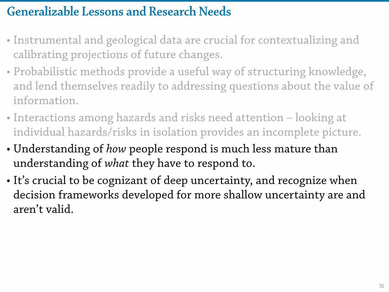
Generalizable Lessons and Research Needs
• Instrumental and geological data are crucial for contextualizing and calibrating projections of future changes.
• Probabilistic methods provide a useful way of structuring knowledge, and lend themselves readily to addressing questions about the value of information.
• Interactions among hazards and risks need attention – looking at individual hazards/risks in isolation provides an incomplete picture.
• Understanding of how people respond is much less mature than understanding of what they have to respond to.
• It’s crucial to be cognizant of deep uncertainty, and recognize when decision frameworks developed for more shallow uncertainty are and aren’t valid.

71
Risk communicationsHow do we translate science to action?
72

Background
From “Consensus Statements White Paper” “While probabilistic projections are sought proactively by some, in many instances they are arriving on the desks of planners, engineers, and decision makers
who have little background in the methodologies used.”
73
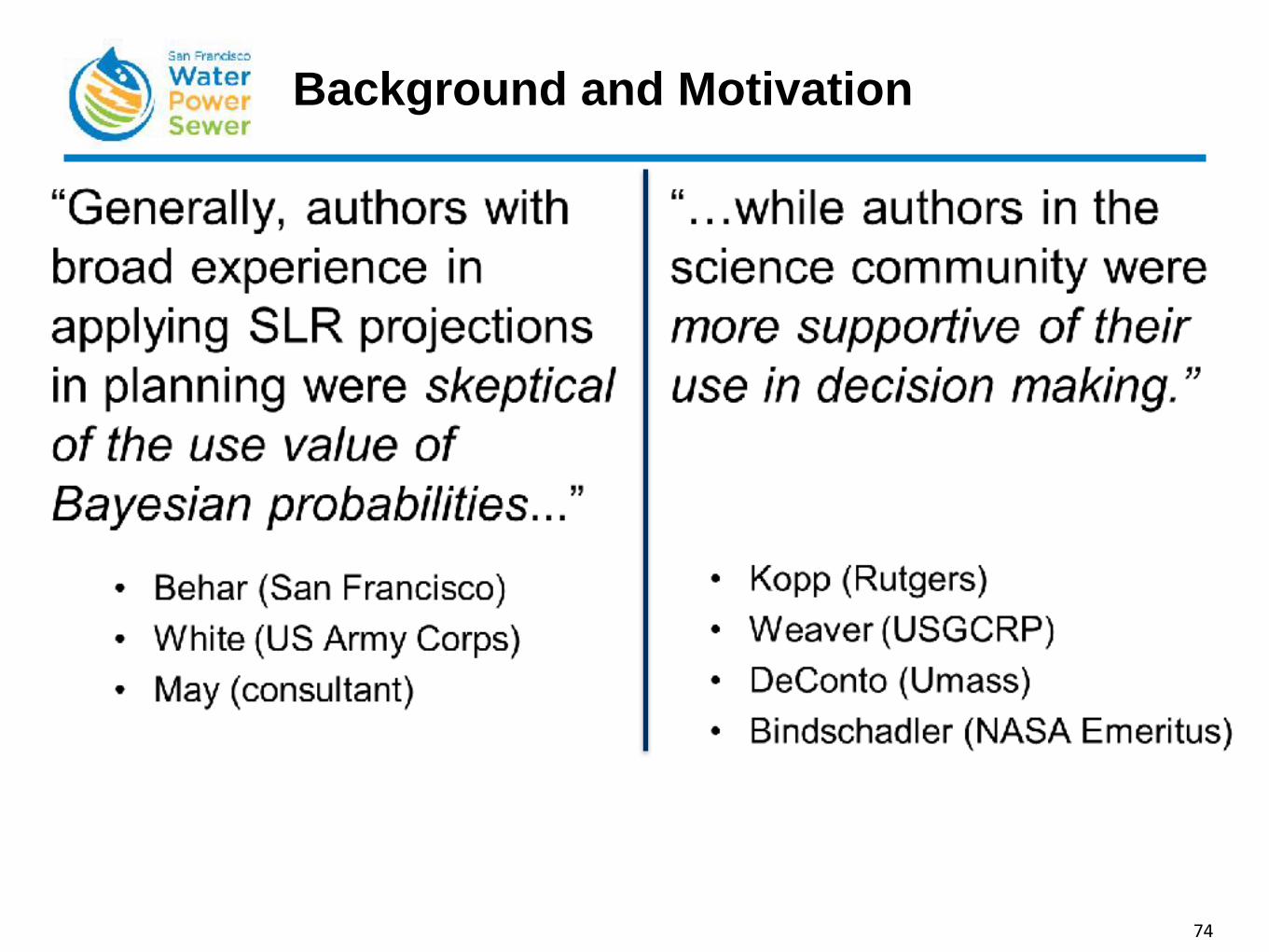
Background and Motivation
74
The Need for Greater Co-Production
“Rigorous co-production efforts related to new SLR science – including probabilistic projections – can and should be much more widespread than they are today.”
“Greater collaboration. . . can reduce the dangers of misunderstanding, misapplication, and maladaptation.”
75

Opportunities Associated with Bayesian Probabilistic Projections
1. “Allows for systematic, reproducible integration of diverse lines of scientific evidence…” and “the ability to clearly demonstrate the sensitivity of the resulting distribution to alternative assumptions about the science.”
2. “Support(s) mapping of global and local SLR scenarios to future emissions pathways” and “Highlights substantial agreement in SLR projections. . . through 2050.”
76
Opportunities Associated with Bayesian Probabilistic Projections
3. “. . . Can, in theory, support a variety of decision frameworks: Expected utility approaches Simplified cost-benefit methods Robust decision making Traditional scenario planning Possibilistic frameworks.”
77

Opportunities Associated with Bayesian Probabilistic Projections
3. “. . . Can, in theory, support a variety of decision frameworks: Expected utility approaches Simplified cost-benefit methods Robust decision making Traditional scenario planning Possibilistic frameworks.”
77
“In practice, users of Bayesian probabilistic projections must understand how Bayesian probabilities differ from the frequentist
probabilities commonly used by decision makers.”

Limitations of Bayesian Probabilistic Projections
1. “There is no consensus on how to meaningfully assign quantitative probabilities for the upper extreme range of potential future global SLR; therefore, a given set of Bayesian probabilistic projections may underestimate or overestimate the SLR contributions due to rapid ice sheet loss after 2050.”
78
Limitations of Bayesian Probabilistic Projections
2. “It is not currently possible to represent uncertainty… with a single Bayesian probability density function after 2050… Therefore, multiple analyses and PDFs should be used in any adaptation study considering projections later this century and beyond.”
3. “The seeming precision of the numbers in a single Bayesian PDF may lead decision-makers to be overconfident about their knowledge of the future.”
79

Limitations of Bayesian Probabilistic Projections
4. “The use of probabilities may lead decision-makers to believe that quantitative probabilities may appropriately be used in the risk assessment equation commonly employed in the engineering community (Risk = Likelihood x Consequence).” “Prior to 2050, the agreement among PDFs may lend confidence to using the probabilities in this manner.”
5. “Supplementary ways of incorporating extreme SLR should also be considered, particularly if the timeframe is closer to 2100 or beyond.”
80

82
Generalizable Lessons and Research Needs
• Instrumental and geological data are crucial for contextualizing and calibrating projections of future changes.
• Probabilistic methods provide a useful way of structuring knowledge, and lend themselves readily to addressing questions about the value of information.
• Interactions among hazards and risks need attention – looking at individual hazards/risks in isolation provides an incomplete picture.
• Understanding of how people respond is much less mature than understanding of what they have to respond to.
• It’s crucial to be cognizant of deep uncertainty, and recognize when decision frameworks developed for more shallow uncertainty are and aren’t valid.
• Co-production is crucial to ensuring that knowledge is useful, and we should be training students to engage in this way.
83
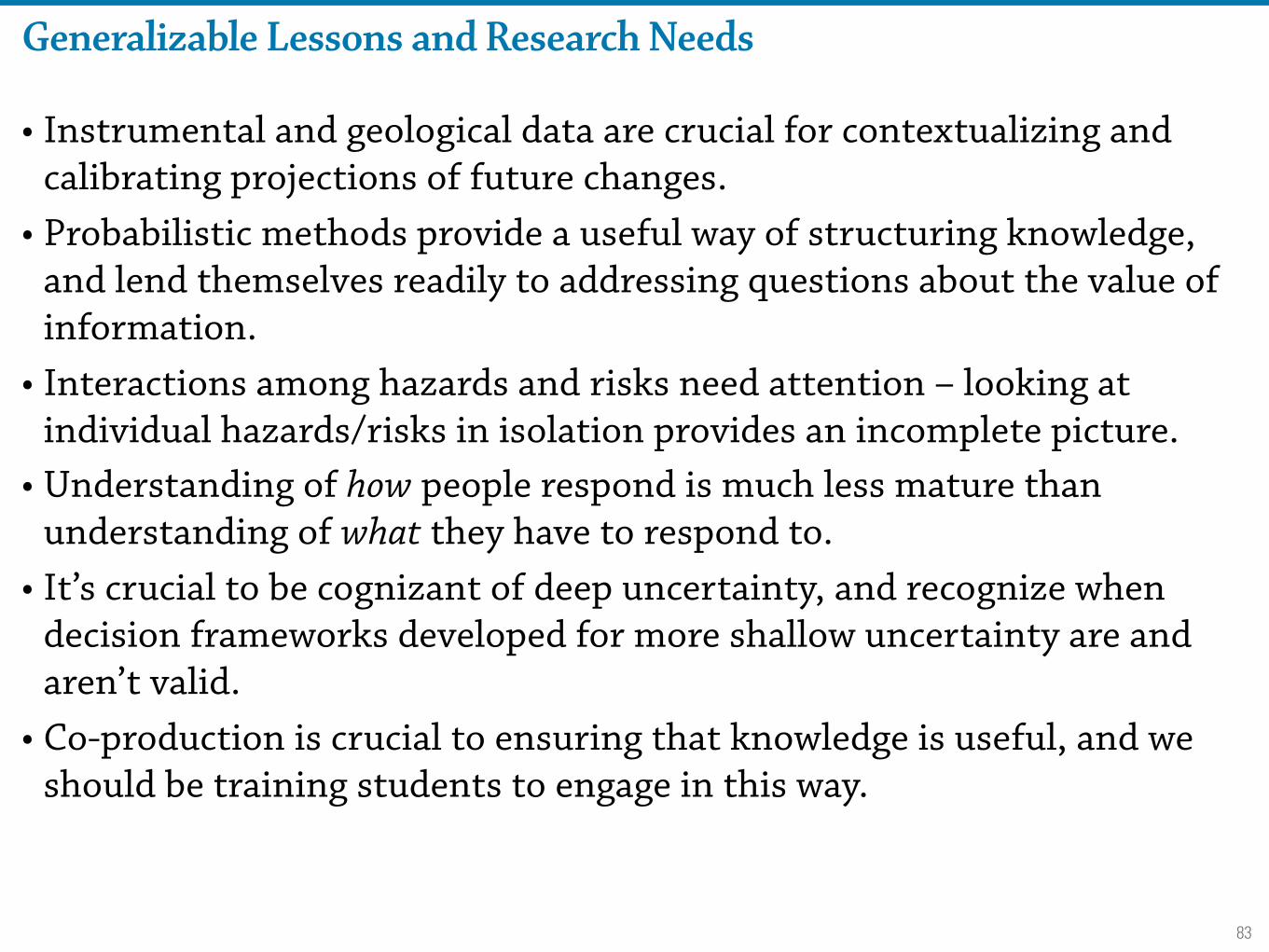
Generalizable Lessons and Research Needs
• Instrumental and geological data are crucial for contextualizing and calibrating projections of future changes.
• Probabilistic methods provide a useful way of structuring knowledge, and lend themselves readily to addressing questions about the value of information.
• Interactions among hazards and risks need attention – looking at individual hazards/risks in isolation provides an incomplete picture.
• Understanding of how people respond is much less mature than understanding of what they have to respond to.
• It’s crucial to be cognizant of deep uncertainty, and recognize when decision frameworks developed for more shallow uncertainty are and aren’t valid.
• Co-production is crucial to ensuring that knowledge is useful, and we should be training students to engage in this way.
Managing climate risk: Rising seas and coastal flooding
as a case study
Department of Earth and Planetary Sciences Institute of Earth, Ocean and Atmospheric Sciences
Rutgers University–New Brunswick
! [email protected] / ! @bobkopp
Robert Kopp
Princeton STEP March 26, 2018

85