beamstrahlungandqedbackgrounds at future linear colliders

SLAC - 371 UC - 414 (T/E/A)

BEAMSTRAHLUNGANDQEDBACKGROUNDS AT FUTURE LINEAR COLLIDERS"

Daniel V. Schroeder

Stanford Linear Accelerator Center

Stanford University

Stanford, California 94309

October 1990

Prepared for the Department of Energy under contract number DE-AC03-76SF00515

Printed in the United States of America. Available from the National Techni- hxkxmatias Service, U-S- Department of Chmnerce, X28.5 Port Royal Road,

Springfield, Virginia 22161. Price: Printed Copy A05, Microfiche A01.

* Ph.D thesis

Abstract

Future electron-positron colliders, with center-of-mass energies above 1/2 TeV, must be of the linear, single-pass type, since the energy loss to synchrotron radiation at a storage ring would be unacceptably high. The single-pass configuration requires extremely dense particle bunches, which will have very strong collective electromagnetic fields. As the bunches cross, the field of each disrupts the other, and the electrons and positrons radiate photons under this transverse acceleration. This radiation is called beamstrahlung. Beamstrahlung can take away a large fraction of the available collision energy at such machines, but it also makes it possible to study electron-photon and photon-photon interactions.

This dissertation is a detailed study of several aspects of beamstrahlung and related phenomena. The problem is formulated as the relativistic scattering of an electron from a strong but slowly varying potential. The solution is readily interpreted in terms of a classical electron trajectory, and differs from the solution of the corresponding classical problem mainly in the effect of quantum recoil due to the emission of hard photons. When the general solution is expanded for the case of an almost-uniform field, the leading term is identical to the well-known formula for quantum synchrotron radiation. The first non-leading term is negligible in all cases of interest where the expansion is valid.

In applying the standard synchrotron radiation formula to the beamstrahlung problem, the effects of radiation reaction on the emission of multiple photons can be significant for some machine designs. Another interesting feature is the helicity dependence of the radiation process, which is relevant to the case where the electron beam is polarized.

The inverse process of coherent electron-positron pair production by a beamstrahlung photon is a potentially serious background source at future colliders, since low-energy pairs can exit the bunch at a large angle. Pairs can also be produced incoherently by the collision of two photons, either real (from beamstrahlung) or virtual (emitted by a passing electron or positron). The rates, spectra, and angular distributions for both the coherent and incoherent processes are estimated here. At a 1/2 TeV machine the incoherent process will be more common, resulting in roughly lo6 pairs per bunch crossing. One member of each pair is always pushed outward, at an angle determined by its energy, by the field of the oncoming bunch. In addition, a small number of pairs are initially produced with a comparable or larger angle.

.. 11

Acknowledgments

It is a pleasure to thank the many people who have made this work possible: Dick Blankenbecler, my advisor, for his endless ideas, help, and encouragement

during the last four years. None of this could have been done without him. Michael Peskin, for his encyclopedic knowledge and enthusiastic answers to the

most mundane questions, and for going over this entire thesis with a fine-toothed comb when he didn’t have read it at all. Also, of course, for letting me help him with his field theory textbook.

The other three members of my oral examination committee: Sid Drell, Lenny Susskind, and Helmut Wiedemann, for their excellent questions and helpful comments.

Stan Brodsky, Russel Kauffman, and Eran Yehudai, who each provided essential help with parts of this thesis, and all the rest of the SLAC theory group, for making it a great place to work.

Pisin Chen, one of the world’s real experts on beam-beam interactions, for hours of essential discussions during the last few months, during which I learned how complicated this subject really is.

Bob Palmer and Ron Ruth, for being the experts that they are but still taking the time to answer my questions.

The organizers of and participants in the 1990 Snowmass conference, where the work of Chapter 7 was done; especially Dave Burke, for inviting me; Ghislain Roy, for his computer and his company; and (most of all) John Irwin, for getting us the best condo at Snowmass and teaching me so much while we were there.

Many others have contributed to this work in a less direct way. I am extremely indebted, in the literal sense, to the taxpayers of the United States, for paying my munificent salary during the last four years. Meanwhile, support of another sort has come from many friends, neighbors, .and roommates at Stanford, especially Ned Gulley, Karin Pagel, Daniel Pierce, Jonathan Pila, and Dave Shortt. And of course I owe everything to my parents, Vernon and Dorothy Schroeder, who have tried so hard for all these years to understand why their son wants to be a physicist.

... 111

.

Contents c

0

r

..

P

1 Introduction . . . . . . . . . . . . . . . . . . . . . . . . . . 1 2 Machine Parameters . . . . . . . . . . . . . . . . . . . . . . 2

3 Classical Beamstrahlung . . . . . . . . . . . . . . . . . . . . 6

3.2 Classical Synchrotron Radiation . . . . . . . . . . . . . . . . 8 3.3 Application to Specific Bunch Geometries . . . . . . . . . . . 10 3.4 Radiation Reaction . . . . . . . . . . . . . . . . . . . . . 13 3.5 Limit of the Classical Regime . . . . . . . . . . . . . . . . 14 3.6 Luminosity Spectrum . . . . . . . . . . . . . . . . . . . . 15 3.7 Number of Photons Radiated . . . . . . . . . . . . . . . . . 17

4 Quantum Beamstrahlung: Formalism . . . . . . . . . . . . . 20 4.1 General Treatment of Radiation in an Extended Field . . . . . . 20 4.2 Connection with Classical Radiation Formulae . . . . . . . . . 27 4.3 Expansion for an Almost-Uniform Bunch . . . . . . . . . . . 30 4.4 Dirac Electrons . . . . . . . . . . . . . . . . . . . . . . . 34 . 4.5 First Correction for a Nonuniform Bunch . . . . . . . . . . . 39

5 Quantum Beamstrahlung: Applications . . . . . . . . . . . . 45

5.1 Properties of Quantum Synchrotron Radiation . . . . . . . . . 45 5.2 Beamstrahlung from Polarized Electrons . . . . . . . . . . . . 51 5.3 Multiple Photon Emission . . . . . . . . . . . . . . . . . . 53 5.4 Numerical Computation of the Multiple-Photon Spectra . . . . . 57 5.5 Luminosity Spectra . . . . . . . . . . . . . . . . . . . . . 63

6 Coherent Pair Production . . . . . . . . . . . . . . . . . . 69

7 QED Backgrounds at the Next Linear Collider . . . . . . . . 77 7.1 Outgoing Angles and Interaction Region Geometry . . . . . . . 77 7.2 Coherent Pair Production . . . . . . . . . . . . . . . . . . 82 7.3 The Breit-Wheeler Process, yy 4 e+e- . . . . . . . . . . . . 84 7.4 The Bethe-Heitler Process, e y ee+e- . . . . . . . . . . . . 89 7.5 The Landau-Lifshitz Process, ee -+ eee+e- . . . . . . . . . . . 91 7.6 Other QED Backgrounds . . . . . . . . . . . . . . . . . . 92

. . . . . . . . . . . . . . . . . . . . . . . . . . 3.1 Disruption 6

References . . . . . . . . . . . . . . . . . . . . . . . . . . 94 il

.

iv

1. Introduction Y

.. ‘ Consider a hypothetical electron-positron collider with.a’center-of-mass energy

of 1/2 TeV or more. Synchrotron’radiation would make a storage ring of this energy impractical, so such a machine would have to consist of two linear accelerators, aimed at each other. Since each pair of bunches has only one chance to cross and interact, the luminosity per pulse must be very high. The electromagnetic fields inside the electron and positron bunches would be very strong, causing the particles to bend inward as the bunches cross (this phenomenon is called disruption). As they bend, the particles emit synchrotron-like radiation, called beumstruhlung.

The phenomenon of beamstrahlung was recognized several years ago!” Much work on the subject has been done in the last few motivated by the serious attention now being given to future linear colliders and the large effect that beamstrahlung will necessarily have on their performance. Most recently, the inverse process of electron-positron pair production by beamstrahlung photons has been recognized as a source of potentially serious detector backgrounds, and has also received a great deal of attention.

IlO.111

[12-14]

This dissertation treats many aspects of the beamstrahlung and pair production processes, both formal and practical. It is intended as a pedagogical review of the subject, and no prior knowledge of these phenomena is assumed.

Chapter 2 briefly describes the relevant parameters for two specific hypothetical machine designs, for use in later examples throughout the paper. Chapter 3 is a detailed review of the beamstrahlung process, simplified by the use of classical radiation formulae. Both of these chapters should be of general interest.

Chapter 4 then delves into formalism. It contains a derivation (based on the work of Blankenbecler and Drell[5’71) of the standard formula for quantum synchrotron radiation, and also of a generalization of this formula to motion in nonuniform fields. The first correction in field gradients to the standard formula is computed explicitly, and it is concluded that the standard formula alone is sufficiently accurate in all cases of interest.

Chapter 5 uses the standard formula to compute the electron and photon spectra in the presence of beamstrahlung, including the effect of radiation reaction on subsequent radiation. This part of the paper follows the outline of Ref. 8, sup- plying more details on the shapes of the spectra in different regimes. Here we also examine the polarization of the electrons and photons in the case where the incoming electron beam is longitudinally polarized.

The inverse process of coherent pair production is discussed briefly, with an emphasis on applications, in Chapter 6. Chapter 7 then concentrates on order- of-magnitude estimates of background processes at the next generation of linear

1

colliders. Because of the spectra of the pairs produced, the coherent pair production process is less of a background problem here than the various incoherent processes involving direct collisions of electrons, positrons, and photons. We discuss both the spectra and angular distributions for all of these processes.

2

2. Machine Parameters

Some possible parameters for future linear colliders are listed in Table 2.1. Parameters for the existing Stanford Linear Collider (as projected for 1993-4) are listed for comparison. We will consider two imaginary future machines. The “Next Linear Collider”, with a center-of-mass energy of 1/2 TeV, is now considered an attainable next step beyond the SLC whose design could be complete by 1992. The “Futuristic Linear Collider” is much more hypothetical; its CM energy of 5 TeV would allow it to thoroughly study the energy regime that will be opened by the SSC. Both of these designs are taken from a recent review article by palmer^"] which also contains several other parameter sets, and which explains in detail how the fundamental parameters are chosen.

The NLC design given here (machine G in Ref. 10) represents one extreme in the design of a 1/2 TeV collider. The aspect ratio R is relatively small, and has been chosen to give the highest possible luminosity consistent with a reasonable (but arbitrary) limit of - 0.3 on the fractional energy loss due to beamstrahlung (denoted 6). Other designs in Palmer’s paper have R as high as 180, which yields L ==: 1.4 x cm-2sec-1 and 6 M .04. Since this dissertation is about beamstrahlung, I have chosen the example for which beamstrahlung is most important.

The FLC parameters in Table 2.1 (machine K in Ref. 10) are of course very speculative, but Palmer’s analysis makes it clear the beamstrahlung energy loss is a dominant consideration in any machine with an energy above 1 TeV. To obtain the required luminosity (about lo3* cm-2sec-1 times the square of the energy in TeV) at the lowest possible cost, one is forced to the largest acceptable value of S. We will see, however, that the beamstrahlung photon spectrum is much different at 5 TeV than at 1/2 TeV.

The shapes of the electron and positron bunches at the interaction point are generally assumed to be gaussian; the rms dimensions ox, cy, and crz are listed for each machine in Table 2.1. In much of what follows it will be more convenient to work instead with bunches of uniform density. An “equivalent” machine with uniform cylindrical bunches (of either round or elliptical cross-section) would have dimensions

(All factors have been chosen to keep the mean square distance from the center of the bunch fixed.) For round beams we will use the symbols B = B, = By and Ob = 6% = Oy.

3

Table 2.1. Machine Parameters

SLC NLC FLC E,, (TeV) 0.1 0.5 5 L (cm-2sec-1) 2 X 1030 9 x 1033 3 x 1035

5 x 1o1O 1

120 .lo5

1.5 X 1 0 - ~ 1.5 X 10-4

1 0.7 1.9

.002 1 .o

4.5 x 10-4 4.5 X io-* 4.5 x 10-4 -

-

1.67 x 10” 10 130 .011

6.5 X 1 0 - ~ 1.7 X 1 0 - ~

25.5 19 3.4 .56 6.0 -78 .26 .2 1 2 6 .35

-215 x 10” 125 170 .002

2 x 10-8 2.7 x

136 9

2.07 25 4.7 27 -24 .22 .26 .26

The first nine parameters, except for L, are taken from Ref. 10. The rest are computed in terms of fundamental parameters as explained in the text.

The luminosity per bunch crossing is given approximately by

where N is the number of particles per bunch. This formula is approximate because of disruption: the bunches “pinch” inward as they cross, increasing the luminosity by a pinch enhancement factor HD. The actual luminosity of the collider is therefore

where f is the frequency of collisions. The NLC and FLC designs employ groups 1

of 10 and 125 closely spaced bunches, in order to extract more of the RF energy; thus the collision rate f at these machines is equal to the number of bunches (Nb) times the “repetition rate” listed in Table 2.1.

4

e

e

The remaining quantities listed in Table 2.1 will be defined and discussed later in this paper. In brief, they are as follows. The disruption parameter, D,, is a dimensionless measure of the amount of pinching (in the vertical .dimension). The classical or quantum nature of the beamstrahlung is determined by T; when T 2 1, individual photons carry away a significant fraction of the beam energy and classical radiation formulae break down. The number of photons emitted by each electron, in the classical limit, is given by NZ. (The previous two quantities are depend on position within the bunch, and are here evaluated for an electron at the edge of a uniform cylindrical bunch.) Finally, S is the average fractional energy loss due to beamstrahlung. It is computed here in five approximations, as discussed in Sections 3.3 and 5.4.

.

5

3. Classical Beamstrahlung

Almost all aspects of beamstrahlung can be understood classically. Before plunging into a full quantum-mechanical treatment, therefore, we will carry out a detailed classical analysis of the problem in this section. In the next section we will see that quantum effects, though numerically large, can be incorporated with little additional difficulty.

3.1. Disruption

First consider only the motion of the electrons and positrons, in the absence of radiation. As the bunches pass through each other, the particles bend inward, due to the attraction of opposite charges. This phenomenon is called disruption. It is most easily understood by working in the rest frame of one of the bunches, where there are no magnetic forces between the bunches. In the rest frame of the positrons, the length of the positron bunch is L = yL,, - 100 meters. (The symbol y will always denote the length contraction factor in the CM frame of the colliding bunches.) Since the final-focus area and interaction region are length- contracted by y, only a tiny fraction of the positron bunch is focused at any given time. The electrostatic repulsion within the positron bunch therefore has a negligible effect. An oncoming electron, however, traverses the entire length of the positron bunch when it is fully focused; the electron is therefore bent inward by a significant amount. Furthermore, since the length of the electron bunch is L / ( 2 r 2 ) , the electric field due to the electrons is 2y2 times stronger than that of the positrons and therefore the positrons are severely disrupted as well. (In the laboratory frame where both bunches are moving, each bunch has a magnetic field that is nearly equal in magnitude to its electric field. The electic and magnetic forces within a moving bunch nearly cancel, while its electric and magnetic forces on the oncoming bunch add.)

To understand disruption more quantitatively? consider a single electron passing through the positron bunch. First assume, for simplicity, that the bunch is a uniform cylinder, and that the electron enters parallel to its axis with impact parameter bo. To a first approximation, we can assume that the positron bunch is stationary. Neglecting end effects, the electric field is then

E(b) = -21/ob, N a

where Vo E - LB2

(We use units in which li = c = 1 and CY = e2/47r. A factor of - e / 4 ~ has been absorbed into E; in other words, E is really the force felt by the electron.) The

6

electron’s trajectory is therefore

where

is a dimensionless measure of the disruption. (Here re = 2.82 X cm is the classical electron radius.) If D << 1, the distortion of the pulses is very slight.

For flat bunches we must define two disruption parameters, D, and D,. Con- sider a uniform bunch with elliptical cross-section. The electric field inside is[151

X Y 2Na Bz BY L(B, + B y )

E, = -2f i - , E, = -2Vl-, where VI = . (3.4)

By considering the “wavelength” of the path of an electron along either axis of the bunch, we arrive at the definitions“‘]

4NaL 2Nr,a, B D, = - - D, = AD,. ( 3 . 5 ) f i m ~ ~ By ( B, + BY) YUY + CY ’ Bz

The values of D, for the SLC, NLC, and FLC are listed in Table 2.1. In order to maximize the pinch enhancement, D (or for flat beams, Dy) should lie roughly in the range from 1 to 20. (The luminosity enhancement factor H D depends on the bunch length, the depth of focus at the interaction point, and any offset in the beam positions, as well as on D. The only known method of computing H D reliably when D is large is by computer simulation.)

117,181

When D 2 1, the effect of disruption can be computed analytically. Expanding the trajectory (3.2) to lowest order in D and averaging over the collision time, we find that the average dimension of the bunch is reduced by a factor of

Ueffective - D - 1 - - + S ( D 2 ) . U 4&

Although this formula does not apply to the vertical disruption of machines like the NLC and FLC, it is quite accurate for the much smaller horizontal disruption.

7

3.2. Classical Synchrotron Radiation

As the electrons undergo this transverse acceleration, they radiate photons; this radiation process is called beamstrahlung. The amount of beamstrahlung radiation is conventionally characterized by the average fractional energy loss, 6. We normally want S to be small.

We can easily make a classical estimate of 6. At any point r along its trajectory, an electron feels an electric field E(r) , and its trajectory can be approximated as a circle with radius

I

n

(3.7) .

where p = 2y2m is the electron's momentum. Since the trajectory is circular we can now apply the standard formula"g1 for synchrotron radiation:

00

d l - = 2ha-- / d<K513(<). P W

dw m WC 2w/wc

Here w is the frequency of the radiation, wc is the critical frequency,

w =-- 3P3 3P2 IE(b)l c - -

m3p m3 9

and I is the energy radiated by the electron during one revolution about the circle. Over any small distance AZ the electric field is approximately constant, and

the electron travels a fraction (Az)lE1/2np of a revolution, so for classical beamstrahlung,

(3.10)

2 w j w c

Since the modified Bessel function diverges as ( + 0, it is more convenient to write this formula in terms of the Airy function:"']

00

_ - d l am2(Az)w J (: ) dw

- dv - - 1 Ai(v), P2

U

where

(3.11)

(3.12)

A plot of the Airy function is shown in Fig. 3.1. The spectrum extends out to w - WC, beyond which it falls off exponentially according to the fall-off in the Airy

8

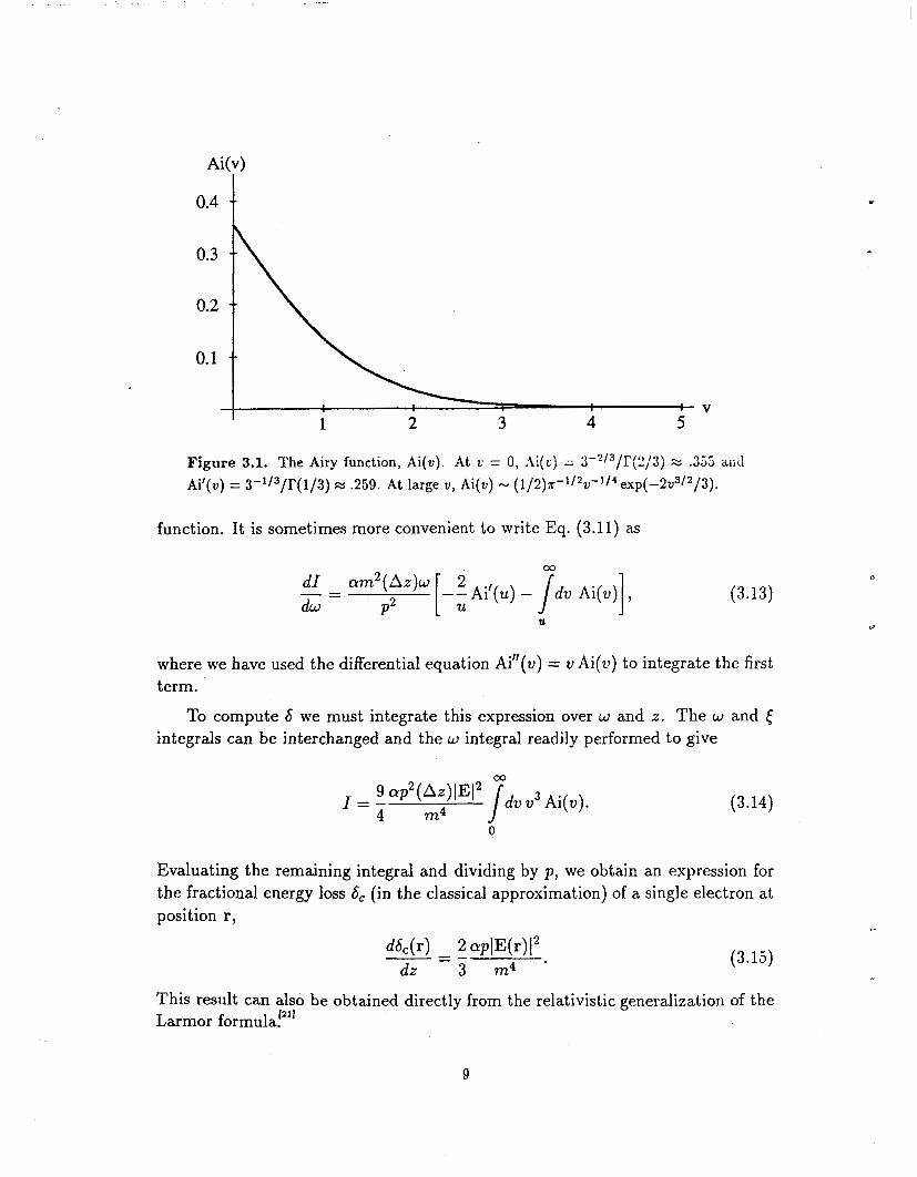
Ai(v)

0.4 --

: v 1 2 3 4 5

Figure 3.1. The Airy function, Ai(v). At u = 0, ,2i(c) ;= 3-'/'//r(2/3) z .355 &lid Ai'(v) = 3-'l3/r(1/3) x .259. At large v , Ai(v) - (1/2)7r-'/*~-'/~ exp(-2~' /~/3) .

function. It is sometimes more convenient to write Eq. (3.11) as

d l crm2(Az)w - = dw P2

U

(3.13)

where we have used the differential equation Ai"(v) = vAi(v) to integrate the first term.

To compute S we must integrate this expression over w and z. The w and ( integrals can be interchanged and the w integral readily performed to give

(3.14)

Evaluating the remaining integral and dividing by p , we obtain an expression for the fractional energy loss 6, (in the classical approximation) of a single electron at position r,

(3.15)

r

This result can also be obtained directly from the relativistic generalization of the Larmor formula!"

9

The classical synchrotron radiation formula (3.8) follows from a much more general formulayzl which includes the angular and frequency distributions for classical radiation from a charge undergoing an arbitrary accelerated motion:

(3.16)

Here #3 is the particle’s velocity vector, and k is a unit vector pointing from the particle to the (distant) observation point. In the next chapter we will see that this general result, and also the specific formula (3.11)) have simple counterparts in quantum mechanics.

3.3. Application to Specific Bunch Geometries

Let us assume that the disruption is negligible, and that the bunches are uniform in the z-direction. Then the electric field felt by any electron is constant over the length L of the bunch, and depends only on its impact parameter b. Thus Eq. (3.15) becomes

(3.17)

The subscript ‘c) denotes ‘classical’, while ‘1’ signifies that this formula is a first approximation, obtained by neglecting radiation reaction ( i e . , the dependence of p on z).

For a round cylindrical bunch shape we can use expression (3.1) for the electric field to obtain

8 cr3N2pb2 3 m4LB4 &l(b) = -

Averaging over impact parameter gives

(3.18)

(3.19)

Note that it is possible to have large disruption with negligible beamstrahlung, or vice versa.

Next consider a uniform bunch with elliptical cross-section. According to Eq. (3.4)) the magnitude of [El is constant on any interior elliptical surface; it

10

depends only on the quantity x2 y2 -+- B,2 Bi’ (3.20)

and is less than at the corresponding point within a round bunch of the same cross-sectional area by a factor of

(3.21)

Since Scl is proportional to E2, the average fractional energy loss of an electron going through a uniform elliptical bunch is

(3.22)

This is the formula used to compute the values of SC1 listed in Table 2.1. Nearly all proposed machine designs have a very large value of the aspect ratio

R = a,/oy; in this case field strength (and hence the beamstrahlung energy loss) is independent of oy. This simplification is fortunate for our treatment of beamstrahlung, since the effective value of oy changes significantly in the presence of disruption. Although the distortion of the bunches under large disruption is much more complicated than a mere reduction in by, at least this leading-order effect can be neglected in beamstrahlung computations. Unfortunately, the particular NLC design given in Chapter 2, with its unusually small aspect ratio of 25, has a non-negligible horizontal disruption as well. The effect of this horizontal disruption is neglected in all the calculations and plots of this paper, but is discussed at the end of Section 5.4.

Real bunches are of course very different from ideal uniform cylinders, but the nonuniformities have little effect on 6. Suppose, for example, that the bunch is uniform in the z direction, but gaussian in b (with cylindrical symmetry). The charge density is then

The electric field (ignoring end effects) is therefore

(3.23)

(3.24)

From this we can compute &(b) from Eq. (3.17).

11

Now the question arises, what is the proper way to average over impact parameter when the charge density is not uniform? TO compute the average energy loss by an electron we would weight 6(b) by p-(b), the electron charge density. But if we are interested in the electron energy that is available for a subsequent reaction, we should also weight each electron by the probability that it will participate in such a reaction. In other words, we should also weight S(b) by p+(b), the positron charge density. The appropriate average is therefore

(3.25)

For the present calculation we will assume that p-(b) = p+(b) = p( b) (up to a normalization constant that depends on the frame of reference), so the average becomes

(3.26)

For our classical computation, S ( b ) is given by Eq. (3.17). Using (3.23) for the charge density and (3.24) for the electric field, and defining /? = b/B = b/2cq,, we find for a bunch with transverse gaussian profile,

gaussian = 6;;linder 6Cl - e e - ) =bel 2P2 2 cylinder x Slog(9/8). (3.27)

0

The average energy loss is reduced by a factor 81og(9/8) M .942 relative to that for a uniform cylinder.

If, instead of using Eq. (3.26), we were to weight S ( b ) with only one factor of the charge density (and thereby compute the literal average energy loss per particle), we would obtain a factor of 41og(4/3) FZ 1.15 relative to the average (3.19) for a uniform cylinder. Since these two definitions of 6 differ by 21%, it is important to remember, in any calculation for nonuniform bunches, which definition is being used.

Finally, suppose that the bunch has a gaussian profile in the longitudinal direction. Multiply the charge density everywhere by a factor

(3.28)

in the rest frame of the positron keep the total charge fixed.) Since

12

the longitudinal variation is negligible on the scale of the width of the bunch, the electric field is very nearly transverse, and is altered by the same factor. According to Eq. (3.15), the energy loss dS/dz is proportional to the square of this factor,

.

(3.29)

Integrating over z , we find that S is reduced, relative to Eq. (3.17), by a factor of M .977.

3.4. Radiation Reaction

Equation (3.17) and all the results that follow are obviously wrong, since by increasing L sufficiently we could easily make &I, the fractional energy loss, exceed 1. This is because we have neglected radiation reaction.

Accounting for radiation reaction is quite easy. Imagine slicing the bunch into several thin pieces, through which the electron travels in succession. We can use Eq. (3.17) to compute the energy loss within each slice, then subtract the lost energy to obtain the electron's momentum p as it enters the next slice. Taking the continuum limit, we obtain the simple differential equation for the momentum

(3.30)

where po is the electron's initial momentum and 6,l(b) is given by (3.17) (with p = PO). The solution of this equation is

giving a new expression for the fractional energy l0ss,[2~]

(3.31)

(3.32) ..

The symbol 6, denotes the exact classical value of 6 , including the effect of radiation reaction.

13

3.5. Limit of the Classical Regime

Even after accounting for radiation reaction, it is hard to design a machine with E,, X 1 TeV and a tolerably small value of 6,. Fortunately, the beamstrahlung energy loss is further reduced by the effects of quantum mechanics. We can easily see whether our classical computation is valid by looking at the classical spectrum (3.11). The intensity is sizeable for frequencies up to wC. But for an electron at the edge of a uniform elliptical bunch, we have

wc(edge) - - 12pNcr (3.33) P m3L(B, + BY) *

At a machine with sufficiently large energy and/or luminosity, this quantity can easily exceed 1. If we try to interpret the classical spectrum in terms of photons, this says that a single photon can carry away more energy than the electron has. Thus a proper qmntum-mechanical calcuIation is necessary in this case.

It is convenient to introduce a dimensionless quantity Y that characterizes the classical or quantum nature of the radiation. The standard definition is

(3.34)

so the classical results are valid when T << 1. To characterize a machine by a single number we could evaluate Y at a typical point within the bunch. For a uniform elliptical bunch, a suitable characterization would be the value of Y at the edge,

(3 .35 )

(Here X, = l /m = 3.86 x cm is the electron Compton wavelength.) This quantity is listed for each of our machine examples in Table 2.1. Alternatively, following Refs. 5 and 7, we can use the quantity

m3LB C=-, 2pNa (3.36)

which is the reciprocal of Y ( B ) for a round cylindrical bunch. For uniform elliptical bunches, Y(edge) = l /GC. Thus when GC >> 1, the classical radiation formulae are valid, while when GC 5 1, we are in the quantum regime.

14

.

A B C

Figure 3.2. One instant during the crossing of uniform bunches. When the radiation is classical and 6 << 1, the center-of-mass energy of the colliding particles is the same everywhere along the line from A to C.

3.6. Luminosity Spectrum

To the experimental physicists who are using a linear collider, the quantity of most interest is not the electron’s energy loss, but rather the spectrum of relative luminosity as a function of the center-of-mass energy of the colliding particles. In the absence of beamstrahlung this spectrum would be a delta function located at the nominal machine CM energy. In the presence of beamstrahlung the spectrum is smeared toward lower energies.

To obtain a very crude approximation to the luminosity spectrum, let us neglect disruption, radiation reaction, and quantum effects, and assume that 5 is large enough to measure but much less than 1. (These assumptions are almost never met, so the following naive analysis is almost never sufficient. But it is still a valuable departure point for subsequent refinements.) The energy of an electron or positron at any given time then depends only on its impact parameter and on how much of the oncoming beam it has passed through. The situation for cylindrical bunches is shown in Fig. 3.2. Electrons at point A still carry the full beam energy, but the positrons they are colliding with have lost a fraction ( z / L ) b of their energy, where S depends on the impact parameter b. The CM energy e,, of these electrons and positrons, expressed as a fraction of the nominal machine CM energy E,,, is

x=-- ecm - JW M 1 - -5. Z E c m 2L

(3.37)

Electrons farther to the right have lost a small fraction of their energy, but the positrons have lost correspondingly less. At point B, for instance, the electrons and positrons have each lost a fraction (2/2L)6, so the fractional CM energy is still 1 - (2 /2L)S. At point C the positrons have lost no energy, but the electrons

15

1- 6( b) 1

‘i

Figure 3.3. Luminosity spectrum for all particles at a fixed impact parameter, in the classical regime, for 6 << 1. The average fractional loss in the CM energy is 6(b)/2.

have lost a fraction ( z / L ) S , so the CM energy is again given by (3.37). In the limit where 6 is small, all collisions at this instant and at a fixed impact parameter have the same CM energy.

The relative amount of luminosity that comes from this instant is proportional to z. As z increases, the luminosity increases linearly, as does the CM energy loss, until the bunches overlap completely. The CM energy loss then continues to increase linearly as the amount of overlap, and hence the luminosity, decreases. At the last moment of overlap, the fractional CM energy reaches its minimum value, 1-6. For a fixed value of the impact parameter, therefore, the luminosity spectrum has the triangular shape shown in Fig. 3.3. In particular, the mean loss in CM energy is 6(b)/2. (When 6(b) is finite, the mean loss in CM energy is slightly more.)

Now consider the effect of changing the impact parameter. Near the axis of the bunches the energy loss is small, but there are relatively few particles. Away from the axis the energy loss and the number of particles both increase. Computing a properly weighted average of the luminosity spectrum over impact parameter (for a round or elliptical bunch), we obtain

(3.38)

16

- x

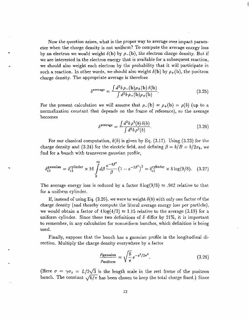
Figure 3.4. Luminosity spectrum, averaged over impact parameter, in the classical regime, for 6 << 1. The average fractional loss in the CM energy is haverage/2.

This result is plotted in Fig. 3.4. Here Smax is the maximum value of 6, that is, the energy loss of an electron at the edge of the bunch. The average value of 5, as we computed in Eq. (3.22), is Sm,x/2. The mean fractional loss in the CM energy is 6,,,/4, half the average value of 6. The luminosity spectrum is quite broad in the classical case, since every electron and positron is continuously losing energy during the bunch crossing. In the quantum case, where radiation is a probabilistic process, and situation is quite different: there is often a considerable peak in the spectrum at X = 1.

3.7. Number of Photons Radiated

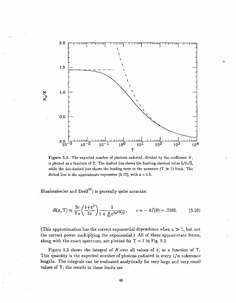
Before discussing quantum beamstrahlung, we can extract one more piece of information from the classical result (3.11). If we assume that the radiation is made up of photons with energy w , then the classical expectation for the total number of photons is

03 00

N,‘ = J d w --z 1 dI = J d w am $ J d v (F - 1) Ai(v), (3.39) dz

P 0 U

where u = (m3w/p21E1)2/3. Interchanging and evaluating the integrals, we obtain

n

(3.40)

17

e

Notice that this expression is independent of p , and therefore independent of radiation reaction. For an electron at the edge of an elliptical bunch,

(3.41)

where G is the ratio defined in Eq. (3.21) (equal to 1 for round bunches) and we have introduced the dimensionless quantity

(3.42)

from Ref. 5. The values of @(edge) for the SLC, NLC, and FLC a.re listed in Table 2.1.

We can interpret y / G as follows. The radiation emitted by a relativistic electron is contained in a forward-pointing cone opening at an angle - r n / p . As the electron curves along its trajectory, the radiation emitted from two different points will overlap only when the transverse momentum acquired by the electron between the two points is less than m. The maximum distance between two such points is called the coherence length, and is given by

m lcoh = (3.43)

Numerically, it is generally the case that lcoh << L. For an electron at the edge of an elliptical bunch,

(3.44)

Thus y / G is approximately the number of coherence lengths in the length of the bunch. Our result (3.40) for the number of photons radiated can alternatively be writ ten

(3.45)

and says that the probability of radiating a photon within one coherence length is roughly a. Note that y >> 1 for any reasonable set of machine parameters, since y = ( a / m ) m , and any linear collider must have a large luminosity per bunch.

18

If N7 were always much less than 1, then S could be calculated directly from the probability P(w) of emitting a single photon with energy w:

61 = 1 Jdw"P(W). (3.46) P

When N7 2 1 and S N 1, this expression gives only a first approximation to 6. The true value of 6 can then be obtained just as in the classical radiation reaction computation above: Divide the bunch into several short slices, and apply the one- photon result to each slice. This procedure is always valid, since N y << (L/Zcoh); we can make the slices small enough that the probability of radiating more than one photon per slice is negligible, but still make the slices larger than the coherence length.

19

4. Quantum Beamstrahlung: Formalism

e

. Let us now turn to the problem of quantum beamstrahlung. We will derive

several expressions for the probability that an electron, while traveling through a bunch of positrons, will radiate a photon. Some of these expressions will be more general, while others will be more useful. All of them, however, will be closely analogous to the corresponding classical results reviewed in the previous section. Our methods will be similar to those of Ref. 5 in many ways. Even those parts of the calculations that are identical, however, are repeated here for completeness.

4.1. General Treatment of Radiation in an Extended Field

Our starting point is the distorted-wave Born approximation,[2*’ in which part of the interaction (the emission of photons) is treated to lowest order only, and the rest (the interaction between the electron and the positron bunch) is treated exactly. Thus our first simplifying assumption is that only a single photon is emitted. In this approximation the matrix element is

where $: and $7 are the initial and final electron wavefunctions in the presence of the external potential, satisfying outgoing and incoming boundary conditions, respectively, and Hint is the interaction Hamiltonian for emission of a photon. The matrix can be represented by a Feynman diagram, shown in Fig. 4.1. Explicitly, for scalar electrons,

where k is the momentum of the photon and e is its polarization vector. We will work with scalar electrons for now, postponing the generalization to Dirac electrons until the end of this section.

Approximate Wavefunctions for Small Disruption

Our first task is to evaluate the wavefunctions $: and $7. Each must satisfy the Klein-Gordon equation,

20

Figure 4.1. Feynman diagram representing the matrix element (4.1) for the beamstrahlung process. The x’s on the electron lines signify that the electron interacts with a strong external field, and its wavefunction is “distorted” accordingly.

then the phase function 4(r) satisfies

( E - V(r)I2 - m2 - IV4(r)l2 + ;024(r) = 0. (4.5)

Of course we cannot solve this equation exactly for any realistic potential. We therefore make the high-energy expansion

for each wavefunction. The first term represents the free-particle plane wave solution, while the second term (xo) gives the usual eikonal approximationfZS1 For our problem it will be necessary to keep x1 as well, since terms of lower order in l/lpl will cancel in the squared matrix element. We may discard x2, however, since it gives only a small correction to the amplitude of the the wavefunction.

For the initial wavefunction we have pi = ( p i , p ) , where p = 2y2m is the initial energy of the electron. (We assume that the longitudinal components of pi, pf, and k are all much larger than their transverse components.) Plugging (4.6) into (4.5) then gives

21

The limits on the integrals are determined by the “outgoing” boundary conditions: The wavefunction must be a simple plane wave as z -+ -w. Since VLV = -E l , we can write the phase of the initial wavefunction explicitly as

4; = p z + p i b - 1 dz’ V(b, z’)

-m

The phase of the final wavefunction can be found in the same way. Let x be the fraction of its energy that the electron keeps:

c#f = XPZ + p i - b + dz’ V(b, 2’) J

We can now check to see when our expansion in powers of l / p is valid. For an electron at the edge of a round cylindrical bunch (with E l given by (3.1)), the ratio of the O(p-l) terms to the O(po) terms in these expansions is roughly

L3V:B2p-’ LNcv L b B2

--N - PB2 D, (4.11)

where D is the disruption parameter (3.3). We are therefore assuming in two places that the disruption is small: in approximating the electric field of the positrons as fixed, and in making the expansion in powers of D.

With these expressions for the wavefunctions, the matrix element (4.2) takes

22

the form

(4.13)

(It will not be necessary to retain the O(l/p) terms in P.) The total phase can be written as

4tot(b, z ) = -q - r - i d z ‘ V(b, z’> + O(l/P), (4.14)

where q = pf + k - p; is the momentum transfer from the pulse, and the O(l/p) terms are given by (4.8) and (4.10).

Stationary Phase Evaluation of the Transverse Integral

-ca

The second term of the total phase changes very rapidly as b varies: For a pulse of length L and diameter B, the potential is typically - IVab2/LB2, so that

M

Vl / d l ’ [-V(b,z’)] N - Ncu 1 B B >> -. (4.15)

-ca

We can therefore evaluate the b integral by the method of stationary phase. The only appreciable contribution comes from the stationary point bst, defined by

ca

-W

Note that b,t depends on z only through the O( 1 / p ) term (which we Will not need to evaluate explicitly). It will be useful to introduce a symbol, bo, for the z-independent part of bst; that is,

03

gl - 1 dz‘ El(b0,z’) = 0 (exactly). (4.17) -ca

In evaluating the integral over b we obtain a factor

2xi iJ , 3

$et Jdl’ Ib, ’

(4.18)

where the determinant is of the 2 x 2 matrix obtained by setting i and j equal to

23

T

2 or y. We then simply replace b by b,t in the integrand, with the result

We will need to retain the difference between bo and b,t (a quantity of order l / p ) in the phase, but not in the pre-factor.

Since only a small range of b-values contributes to the matrix element for a given value of q l , we can meaningfully say that the electron has a classical trajectory as it travels through the bunch.

Manipulation of the Squared Matrix Element

To make further simplifications we must square the matrix element:

(For notational convenience we define +t,t(z) z 4tot(bst, z ) and P(z) E P(b0, z).) The phase can be simplified by noting that

Explicitly, the derivative is

-m

-m -m

(4.21)

The difference between b,t and bo is significant only in the second and third terms of the first line. Moreover, these two terms cancel to order l/p. The z-dependent part of b,t has disappeared from our expressions, which now involve only bo.

24

It is useful to eliminate qz and pl in favor of other kinematic variables. This f

can be done by using the relations

(4.23)

and pl f - - 41- k l + p;, as well as the relation (4.17) between ql and E l . After a page of tedious algebra one finds

(4.24)

where 2

ky(z) E k l - (1-x) [ p i + J d%’ El(bo,z‘)]. (4.25)

The quantity in brackets is just the momentum of a classical electron at position z ; thus k’, is just the transverse momentum of the photon, minus the transverse momentum that it would have if it were emitted parallel to the electron. Note that all terms in s of lower order than l /p have cancelled, and that the only dependence on z is through k’,-.

-m

We can simplify the outside polariztion factor in (4.20) by summing over the two transverse photon polarization vectors:

(In the second line we have used the relation iz = 1 - lk1l2/2k2.) We need only keep the leading-order terms in Pz and Pl; from Eq. (4.13)’

P z = (1 + s)p;

25

h

c

(4.27) --oo

(That we only need these expressions to leading order in l / p justifies our using bo rather than b,t(z) in the pre-factor of (4.19).) Plugging these expressions into Eq. (4.26), we find simply

4 € * P(21) € - P(z2) = - (1-x)2 k' (21) - kl(Z?),

€

(4.28)

where kk(z) is given by Eq. (4.25). Using Eq. (4.24) for the phase and Eq. (4.28) for the polarization trace, we

find that the squared matrix element (4.20) takes the form

where for notational convenience we define

~ ~ ~ ( 1 - z ) ~ + lk;(z)I2 s ( z ) E

2 4 1 - x)p

2

9 (4.29)

(4.30)

(The lower limit on the integral in the phase is of course arbitrary.) Notice that, due to our expansion in powers of l / p , all dependence on the longitudinal component of the electric field has disappeared; only the transverse component E l enters Eq. (4.29), through its appearance in the definition (4.25) of kl.

Phase Space Integrations

To compute the cross-section for beamstrahlung we must integrate the squared matrix element over the final-state phase space variables. Conservation of energy leaves five unconstrained momentum components, which we take to be k and ql. Thus we have

(4.31)

26

The ql-integral can be changed into an integral over bo using (4.17):

(4.32)

The awkward factor of J 2 in the squared matrix element is exactly cancelled.

If the flux of electrons were uniform over the width of the positron bunch, the probability that any one electron would emit a photon with energy k = (1-x)p would equal do divided by the area over which the electrons were spread. But since our expression for do involves an integral over impact parameter, we can interpret it to mean that the probability for any particular electron with impact parameter bo to emit such a photon is given by the integrand. Thus we arrive at our most general result for the probability P that a scalar electron with impact parameter b will emit a photon with fractional energy (1-x):

dP(b) 00

d2 k l 2

CY -- dx - ~ ~ x ( 1 - x ) ~ /- ( 2 ~ ) ~ / dz k’Jz) exp(i jdz ’ s ( z ’ ) ) , (4.33)

-00 0

where k’,(z) is given by Eq. (4.25), with E l evaluated at the desired impact parameter b. To obtain the expected fractional energy loss S(b) we simply weight this probability by k / p = (1-z):

d v 4 00

d2 k l dx ~ ~ x ( 1 - x ) ~ (27r)2

2 CY --

- J- . J dz k;(z) exp (i I d z ’ s (z ’ ) ) (4.34)

-00 0

4.2. Connection with Classical Radiation Formulae

Equation (4.34) is similar in form to the general classical formula (3.16) for radiation from an accelerated charge:

I I

(4.35)

The factor d 2 k l / p 2 ( l - ~ ) ~ , for instance, is precisely equal to dil when the angle of the outgoing photon is small.

27

To compare the formulae more closely, let us expand the phase and pre-factor of Eq. (4.35) in powers of l / p . The unit vector points in the direction of the photon momentum k, so

The electron’s transverse momentum, to sufficient accuracy, is

(4.36)

(4.37)

and its transverse coordinates can be found by integrating this quantity. Its longitudinal coordinate is

0

(4.38)

in a coordinate system where z ( 0 ) = 0. The product i - r ( t ) in the phase of (4.35) is therefore

The 1 term is cancelled by the t in the phase, leaving only terms of order l / p . We can now substitute t + z to this order. Setting k = ( 1 - z ) p , we find that the phase of Eq. (4.35) is

(4.40)

Except for a missing factor of z in the denominator, this is identical to the phase in the quantum expression (4.34). (See the definition of s ( z ) , Eq. (4.30).)

Now consider the prefactor in Eq. (4.34). Writing out the double cross-product, we have

(4.41)

where p(t) is the electron’s momentum. Here we must keep terms within the brackets proportional to p3 and p 2 , but no smaller. The largest terms cancel,

28

leaving us with

(4.42)

So again, expressions (4.34) and (4.35) agree except for a factor of x.

Reversing the preceding argument, we can write the quantum result (4.34) as

1 - 0 0 I

This agrees with the classical expression (4.35) in the classical limit, where x + 1 (that is, the photons are soft compared to the electron’s energy). Of course our derivation of (4.43) is not valid for a general trajectory r(t); we assumed that the disruption is small, or, roughly, that the electron’s trajectory does not bend enough to carry it into a region where the field strength is significant.ly different from its value along a straight trajectory. Nevertheless it is tempting to speculate that Eq. (4.43) might hold more generally.

Equation (4.43), or something very close to it, appears to have been previ- ously derived, although the references are elusive. Chen and Yokoya[261 quote a formula involving the same phase as in (4.43), but with a pre-factor that is independent of kl. They attribute their formula to Baier and Katkovfa’’ although it does not appear explicitly in that paper. Bell and quote the same formula and attribute it to the textbook of Berestetskii, et . d?] (whose treatment of synchrotron radiation follows Baier and Katkov), although the formula does not appear explicitly there either. Both Refs. 26 and 28 use the formula to derive results in agreement with those of Section 4.5 below. The formalism of Baier and Katkov involves no explicit expansion in powers of the disruption parameter, so their derivation (whatever the result) is probably more general than ours. In any case, Eq. (4.43) has not received the attention it deserves, in light of its very close resemblance to the well-known classical formula (4.35). The present derivation, based on the scattering-theory method of Blankenbecler and Drell, is entirely new, and ha.s the advantage of being very concrete and explicit in its assumptions.

29

4.3. Expansion for Almost-Uniform Bunch

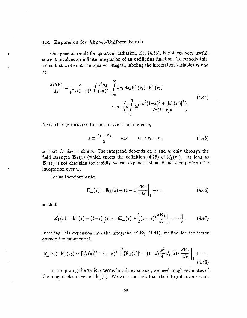
0 Our general result for quantum radiation, Eq. (4.33), is not yet very useful, since it involves an infinite integration of an oscillating function. TO remedy this, let US first write out the squared integral, labeling the integration variables z1 and z2 :

-co (4.44)

x exp(i ] d z I rn2(1-x)2 2x( 1 -x)p t lk1(z’)l2

Next, change variables to the sum and the difference,

zr- zl t 22

2 and w E zz - 22, (4.45)

so that dzl dz2 = dZ dw. The integrand depends on Z and w only through the field strength E l ( z ) (which enters the definition (4.25) of ky(z)). As long as EL(z) is not changing too rapidly, we can expand it about Z and then perform the integration over w.

Let us therefore write

(4.46)

so that

1 k l ( z ) = k;(z) - (1-z) [ (z - z)El(z) + -(z 2 - f)’%/ dz +. - -1. (4.47)

Inserting this expansion into the integrand of Eq. (4.44), we find for the factor outside the exponential,

In comparing the various terms in this expansion, we need rough estimates of the magnitudes of w and k’,(z). We will soon find that the integrals over w and

30

kl are dominated by the regions

(4.49)

For a reasonably smooth bunch shape, we can also approximate

dfdz - 1fL. (4.50)

Thus our expansion is in powers of lcoh/L. This ratio is (almost everywhere) roughly equal to Gfy, or about low3 for the NLC and FLC parameters given in Chapter 2. (Since y is determined by the luminosity per bunch, it must be large for any realistic machine.) By the end of this chapter we will see precisely where our expansion breaks down. Applying the estimates (4.49) and (4.50) to Eq. (4.48), we see that the last term is one power smaller than the first two and can therefore be neglected to leading order.

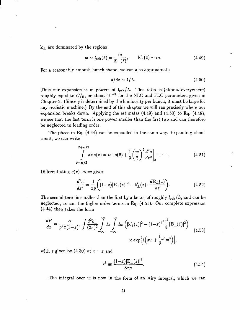
The phase in Eq. (4.44) can be expanded in the same way. Expanding about z = 2, we can write

f - w / 2

Differentiating s ( z ) twice gives

- d2s = -((l-x)lE~(z)12 1 - k',(z). dz2 xp

(4.51)

(4.52)

The second term is smaller than the first by a factor of roughly lcoh/L, and can be neglected, as can the higher-order terms in Eq. (4.51). Our complete expression (4.44) then takes the form

x exp z sw + -r w , ['( 3 "1 with s given by (4.30) at z = Z and

(4.54)

The integral over w is now in the form of an Airy integral, which we can

31

evaluate using the identityL3’]

00

c

(4.55) -m

When powers of w occur inside the integrand, simply differentiate with respect to s and use the differential equation satisfied by the Airy function,

Ai”(v) = v Ai(v). (4.56)

Applying these formulas to Eq. (4.53), we obtain

-m (4.57)

TO perform the integral over k l , we move it inside the z integral, shift from k~ to ky(z), and change to polar coordinates. The angular part is then trivial. TO simplify the integration over the magnitude of kk(z), we change variables to

S v f -.

r

A bit of algebra then reduces our expression to the simple form

dP am2 - - - - J dZ J d v ( - 1) Ai(v), dx P

m m

where

(4.5s)

(4.59)

This is our final result for beamstrahlung from scalar electrons. Notice that when the photons are very soft (that is, (1-x) << l), this definition of u reduces to the classical definition (3.12), and our result (4.59) agrees with the classical synchrotron radiation formula (3.11).

32

It is generally more useful to write the coefficient of Eq. (4.59) in terms of the parameters lcoh and T. Our retult then becomes

d2 P --- - a T d v ( : - 1) Ai(v). dx dz Tlcoh

U

(4.61)

The angular dependence of the radiation is still present in the integrand of Eq. (4.61); v = u corresponds to kl_L(Z) = 0, while v increases as Ikk(E)I increases. Specifically,

V lk>(Z)I2 U rn2(1-x)2' - = 1 + (4.62)

Since the Airy function falls off exponentially when v > 1, this quantity can be large only when u << 1. In this case the 1 term in (4.62) can be neglected. Inserting the definition (4.60) of u, we find that for most values of T, the distribution falls off exponentially when lkk(Z)1 > rn. In other words, the radiation is contained in a cone, centered on the electron's local direction of travel, with opening angle - m / p . When T >> 1, however, this result is slightly modified; the same analysis then shows that the maximum value of lkl_L(Z)l/m is roughly Y113. Up to a possible factor of Y1/3, therefore, our rough estimate for lk;(E)I in Eq. (4.49) is justified. (Recall that even for the FLC parameters in Chapter 2, T1l3 M 3.)

To justify our estimate for w in Eq. (4.49), notice that the integral over w in (4.53) begins to converge when

1 lcoh x 1/3 - - - - = lcohr1/3 (-) . r f i 1-x

(4.63)

So our estimate w N lcoh is valid except when fi is very small. This happens at the extreme soft end of the photon spectrum, and also over most of the spectrum when T >> 1. Neither situation is relevant for most machine parameters, since the quantity Zc0h/L(1-z)1/3 typically remains small until (1-x) - lo-', while T1l3 is quite small in current designs, as noted above. In any case, we have now shown that the estimates (4.49) always give the correct power of lcoh/L, our expansion parameter. We also see that the coefficients in this expansion might very well involve powers of T1/3 and (l-x)'13. In the Section 4.5 we will explicitly compute the next-order term in this expansion, and examine where and how the expansion can break down.

Our earlier expansion in powers of the disruption parameter D is somewhat more troubling. In the phases (4.8) and (4.10) we kept terms through order l/p,

33

. . I

aIld estimated the magnitude of these terms as roughly N a D . Many cancellations have occurred since then, however. All lower-order terms have cancelled, and now we have seen that even the O ( l / p ) terms cannot grow much larger than 1 before the integral over w cuts off. The largest terms of O(1/p2), which we would naively expect to have magnitude NaD2, could exceed the l / p terms even for small D. And as we saw in Chapter 2, D could be as large as 20 at the next linear collider.

Physically, however, we should not expect our results to break down when D is larger than 1 or even 20. The disruption parameter measures the bending of an electron's trajectory on the scale of the length of the bunch, whereas the radiation (at least for small 0) is coherent only over a much smaller scale, Icoh. A breakdown in our formulae for large D could only result from a coherent effect over a large fraction of the bunch length, which seems physically implausible.

These hand-waving comments are of course no substitute for a proper treatment of beamstrahlung in the presence of large disruption. The direct approach of this paper, using explicit wavefunctions, seems very difficult to apply in this case. The only work I know of that may be a.pplicable is that of Baier a.nd I(atko~!'~

4.4. Dirac Electrons

The extension of this derivation to Dirac electrons involves more computation but no new ideas. In this case the matrix element for emission of a photon is

(4.64)

The wavefunctions $: and $7 are solutions of the Dirac equation,

(-icy. v + mP)$ = ( E - V ( r ) ) + , (4.65)

with outgoing and incoming boundary conditions. We will use a chiraI basis for the Dirac matrices:

To find the wavefunctions $: and $7, we write them in the form

(4.66)

(4.67)

where uu and u l a.re two-component spinors and b(r) is the same phase that solves

34

the Klein-Gordon equation. The upper and lower two-component spinors satisfy

[ - i a . ~ + o . ( V 4 ) - ( ~ - ~ ) ] u , + m u l = 0 ,

[ia - V - a (V4) - ( E - v)]q + mu, = 0. (4.68)

Combining these equations and using the fact that d(r) obeys Eq. (4.5), we obtain the second-order differential equations

-

(4.69)

Solving these equations to order l/p, we can easily find the Dirac wavefunctions. Let us introduce the notation v+ E vz + ivy and v- E v, - ivy for the components of any transverse vector v l . We will also abbreviate dz‘ &(b, 2’) as JE*. For the initial state, the phase 4(r) is given by (4.8); the Dirac spinors of definite helicity are therefore

(We use relativistic spinor normalization.) For the final state, the phase 4(r) is given by (4.10), so the right-handed and left-handed spinors are

Since the matrix element involves the same phase as in the case of scalar electrons, the b-integral can be evaluated by the method of stationary phase as before. The rest of our calculation also goes through unchanged, except for the evaluation of the polarization trace. As in Eq. (4.19), the matrix element is

M = i eJ dz E* - P(bo, z ) ei’tot, / but now the vector P(b0, z ) is given by

(4.70)

P(b0,z) = uf*(bo,*) CY ui(bo, t ) . (4.71)

In the Dirac case the photon’s polarization vector is potentially interesting, SO we will not sum over e. Since the photon, initial electron, and final electron can each

35

have two different polarization states, we must evaluate the matrix element for eight different sets of polarizations.

Consider first the case where both the initial and final electrons are right- handed. The components of P(z) are then

(In the last two expressions we have again used p i = q l - k l + p i and Eq. (4.17).) The polarization vector for a right-handed or left-handed photon with momentum k is (to lowest order in small quantities)

1 = - ( l , i, -k+/k) (right-handed) Jz

f i (4.73)

1 or e = - ( l , -i, - k / k ) (left-handed).

It is now easy to work out the polarization-dependent part of the squared matrix element. For a right-handed photon we find

1 4 e - P * ( , I ) e* * P(z2) = - * -

2x ( 1 - x ) 2 + k' (zl)kL(z2). (4.74)

In analogy with Eq. (4.33), therefore, the probability for a right-handed electron to emit a right-handed photon without flipping its helicity is given by

XI 2

d2 kl dx p2x( l -2)3 2x (27r)2

2 Q --

- A /- , (4.75) / d z k i ( z ) exp(i/dz's(r'))

-m 0

where s(z ' ) is defined in (4.30). (Note the close similarity to the corresponding formula for scalar electrons, Eq. (4.33).) Expanding to lowest order in I,,h/L as in

36

the previous section, we obtain the more explicit result W W

d P am2 1 J J (: ) dx p 2x - = -- dz dv - - 1 Ai(v),

-W u

(4.76)

where u is the same as in Eq. (4.60). This is just 1/22 times the corresponding scalar result, Eq. (4.59). By parity invariance, this expression also holds in the case where initial electron, final electron, and photon are all left-handed.

Similarly, if the initial and final electron are right-handed but the photon is left-handed,

(4.77)

The probability for a right-handed electron to emit a left-handed photon without flipping its helicity is therefore given by

z d P

W

Q d2 k l -- dx - ~ ~ ~ ( 1 - 2 ) ~ "JT 2 (2.) / d z k ' ( x ) exp(i/dz's(z'))

-ca 0

Expanding again to lowest order in l c o h / L , this becomes

2

(4.78)

(4.79)

Notice that this is x2 times the above expression for a right-handed photon. Again, this expression also applies to the parity-reversed situation of a left-handed electron and a right-handed photon.

Finally we must consider the case where the electron flips its helicity during the radiation process, say from right to left. The components of P(z) (to order l/p) are now simply

m( 1 -x) im( 1-x) P, = 0, P, = , py = J x f i *

If' the photon is right-handed, we immediately find

2m2( 1 -x)2 € * P*(Zl) €* * P(z2) = ,

X

(4.80)

(4.81)

while if the photon is left-handed, the squared matrix element is zero. The probability for an electron to flip its helicity while emitting a photon (which must have

37

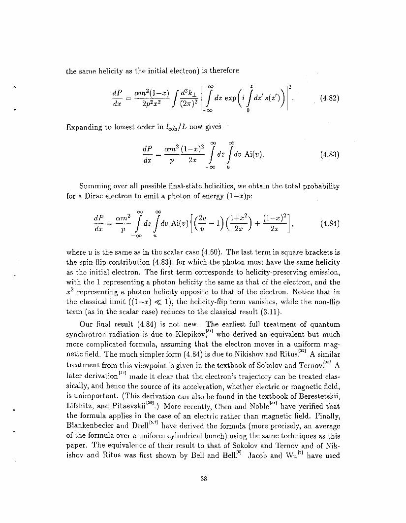
the same helicity as the initial electron) is therefore

c

c

c

dP a m 2 ( 1 - x ) J d 2 k l 7 ( j ) dx 2p2x2

2

-- - ( 2 r 1 dz exp i dz’ s( z’) . (4.82)

-m 0

Expanding to lowest order in l coh/L now gives

dP am2 ( l - ~ ) ~ 7 7 dx P 22 -= - d z dv Ai(v). (4.83)

-m u

Summing over all possible final-state helicities, we obtain the total probability for a Dirac electron to emit a photon of energy (1-z)p:

0 C ) m

-- dP - * / d z / d z . Ai(v) [(E - 1 ) (-) 1 +x2 + (1 -x)2 (4.84) d x P U 22 2x

-m ‘11

where u is the sa.me as in the scalar case (4.60). The last term in square brackets is the spin-flip contribution (4.83), for which the photon must have the same helicity as the initial electron. The first term corresponds to helicity-preserving emission, with the 1 representing a photon helicity the same as that of the electron, and the z2 representing a photon helicity opposite to that of the electron. Notice that in the classical limit ((1-z) << l), the helicity-flip term vanishes, while the non-flip term (as in the scalar case) reduces to the classical result (3.11).

Our final result (4.84) is not new. The earliest full treatment of quantum synchrotron radiation is due to Klepikov:” who derived an equivalent but much more complicated formula, assuming that the electron moves in a uniform magnetic field. The much simpler form (4.S4) is due to Nikishov and Ritus!’] A similar treatment from this viewpoint is given in the textbook of Sokolov and Ternov. later deri~ation”~’ made it clear that the electron’s trajectory can be treated classically, and hence the source of its acceleration, whether electric or magnetic field, is unimportant. (This derivation can also be found in the textbook of Berestetskii, Lifshitz, and Pitae~skii”’~.) More recently, Chen and have verified that the formula applies in the case of an electric rather than magnetic field. Finally, Blankenbecler and Drell[””] have derived the formula (more precisely, an average of the formula over a uniform cylindrical bunch) using the same techniques as this paper. The equivalence of their result to that of Sokolov and Ternov and of Nik- ishov and Ritus was first shown by Bell and Bell!] Jacob and WU[’] have used

(331 A

38

essentially the same method to study the regime where T >> 1. The present paper is the first to apply the scattering-theory formalism of Blankenbecler and Drell to more general bunch geometries for general values of Y, and to derive the local form (4.84) directly by this method.

4.5. First Correction for a Nonuniform Bunch

In Section 4.3 we expanded the integrand of our general formula (4.44) in powers of l coh/L , keeping only the leading order. This parameter is numerically small (typically low3) throughout most of the bunch for any reasonable set of machine parameters. But since lcoh = m/lEll, we should not expect the expansion to converge near the edges of the bunch where the electric field is very small. Furthermore, we saw at the end of Section 4.3 that the true expansion parameter is probably lcoh/Lf i , which is much larger than lcoh/L when (1-2) << 1 or ‘I’ >> 1. It would therefore be a good idea to check the validity of our lowest-order formula, by computing the next-order correction explicitly. We will find that the first nonvanishing correction term is smaller by two powers of lcoh/L.

This correction term for radiation in a nonuniform field was first calculated by Chen and Yokoya:‘] using the formalism of Baier and Katkovr7] The correction term in the limit Y >> 1 has also been calculated by Bell and Bell?” Chen and Yokoya integrated the correction term over and over the photon frequency, and found the result to be negligible compared to the leading term for most sets of machine parameters, but considerable (roughy 30% of the leading term) for a parameter set suggested earlier by Himel and Siegrist?] We will discuss these conclusions at the end of this section.

The computation of the correction term is extremely straightforward, requiring only that we keep higher-order terms when expanding the electric field about z as in Eq. (4.46). It is nevertheless quite tedious, even for scalar electrons. The electric field enters our master formula (4.44) through k’,(z), which appears both in the phase and outside the exponential. It is necessary to keep terms that are smaller than the leading terms by one or two powers of l coh/L , according to the estimates in Eqs. (4.49) and (4.50). It is not hard to see that this is equivalent to reta.ining up to two z-derivatives of E l any given term.

The outside factor, to the needed accuracy, is

64

(4.85)

39

where the dot denotes d/dz, and E l and k', are to be evaluated at z = 2. Higher- order terms'in the phase .are presumably small compared to 1, and can therefore be brought down by Taylor-expanding the exponential. The extra factor we thus obtain is

iw3 . . 1 w3 2 . . ' ' 1 - - k l . E l - -(-kl.El)

24xp . 2 24x13 (4.86) + i w 5 ( 1 - 4 (31ElI2 + 4 E l . E 1 ) + . a m .

1920xp

Expressions (4.85) and (4.86) should now be multiplied together, dropping terms with more than two z derivatives of E l . The resulting expression can be simplified somewhat by noting that terms odd in k l will vanish when we integrate over kk, and that terms of the form (k;.El)2 are, after integration, equivalent to

. I I 2 #,I lEd2* After these manipulations, our expression involves an Sth-order polynomial

in w, multiplied by the same exponential as in Eq. (4.53). The integral over w can again be evaluated in 'terms of the Airy function using Eq. (4.55): and the result simplified using the differential equation (4.56). When the smoke finally clears, we obtain the following expression for the correction term, P2, to the probability of radiation from a scalar electron:

where u is again as defined in Eq. (4.60). We now see explicitly that the ratio of the correction to the leading term (4.61) is of order (!coh/L)2. Furthermore; when u is small, we find that the largest terms in the ratio are of order (rcoh/L&)2, as anticipated in Eq. (4.63). Equation (4.87) actually has a non-integrable singularity at u = 0 (or x = 1). We should not take it too seriously, however, since our expansion in powers of rcoh/L& is not expected to converge in this region. The total energy loss, equal to (1-x) times the above expression, is still finite.

The case of Dirac electrons is entirely analogous. Here we find: for the non-flip radiation probability, and expression identical to (4.87), but multiplied (as was the leading term) by (1+x2)/2x. There is also a correction to the spin-flip term,

It is not hard to check that the sum of the flip and non-flip correction terms agrees

40

precisely with the result of Chen and Yokoyay’ (In the Dirac case there arise additional terms, smaller than the leading term by only one power of Zcoh/L, that are proportional to E l X El. These terms vanish i f the field is always parallel to its z-derivative, or if the bunch has a mirror symmetry and we average over impact parameter, or if we average over the initial electron helicity. Since at least one of these conditions is generally satisfied, we will neglect these terms.)

Let us now consider the total correction to 6, the fractional energy loss. Mul- tiplying Eq. (4.87) by (1-x), and changing variables from z to u , we find

00

-- dS2 dz 30 Jdu (1 + -u3 Ai(u) - 8 Ai(u) - l o ~ A i l ( ~ ) ] -

0

+ [-3u3 Ai(u) + 6 Ai(.)]}. IEL l2 (4.89)

Notice that when T << 1, the factor (1 + Yu3/2)-3 can be expanded and the integrals evaluated explicitly to whatever order desired. The first term in this expansion vanishes identically when integrated, so the integral is proportional to Y when Y << 1. Thus the correction term is very strongly suppressed, relative to the leading term, in the classical limit.

To examine the correction quantitatively, let us specialize to the case of a longitudinally gaussian bunch (but uniform and round in the transverse direction, for simplicity). The electric field is then given by Eq. (3.29):

(4.90)

where u = L/2& = yo, is the length scale in the rest frame of the bunch, and B = 20, is the bunch radius. The ratios that a.ppear in the correction term are

-- 1E1I2 ( z / 4 2 . E l - E1 - (./a)’ - 1 IElI2 - a’ ) IE1I2 0 2

-

Equation (4.89) for the correction to the energy loss therefore becomes

+ C 2 [-4u3 Ai(u) - 2Ai(u) - 10 Ai’(u)] },

(4.91)

(4.92)

where ( = z / o and Y = TOe-c2/’

41

For compa.rison, the leading term (4.59) takes the form

(4.93) We now see explicitly that the ratio of the correction term to the leading term is of order

(4.94)

where y = Na/rnB is the parameter introduced in Eq. (3.41), proportional to the square root of the luminosity per bunch crossing. Since y is large (typically lo3) for any realistic set of machine parameters, the correction term is always negligible near the center of the bunch. On the other hand, no matter how large y is, there is always a (large) value of z / a beyond which the correction is larger than the leading term. For most machines, the correction term will be small even here (compared to the leading term evaluated at z = 0), since Y is suppressed by a factor of e- 2 / 2 2

If Y X 1 even with this suppression, however, the correction term can become large. The condition for this to occur is

YO - X 1 or y C 5 1 , (4.95) Y

where C M l / Y o is the parameter introduced in Eq. (3.36). (These expressions assume round bunches. For elliptical bunches, substitute y + y/G and C --+ CG, where G is the quantity defined in Eq. (3.21), roughly equal to the square root of the aspect ratio. The factors of G happen to cancel in the condition y C 2 1, which still holds.)

Although most proposed machine parameters come far from satisfying condition (4.95), there are exceptions. Following Chen and Yokoya, let us consider the parameters suggested by Himel and Siegrist for a 5 + 5 TeV colljder:

= .98 X lo7;

N = 1.2 X 10';

az = 4 x 10- cm;

ar = 2.5 x 10-8cm.

5 (4.96)

This is a machine with round beams, y = 680, and C = 1.34 X (It relies on a very large value of Y' to suppress beamstrahhg, a quite different philosophy from

42

a

0.03

0.02

0.0 1

0.00

I I I I I I I I I I I I I I

0 2 4 6 z/a

Figure 4.2. The differential fractional energy loss, d b / d ( z / a ) , is plotted against %/a, for the Himel-Siegrist parameters given in Eq. (4.96) and b = or. The solid curve is the correction term (4.92), while the dashed curve is the leading term (4.93). These curves are for scalar electrons.

the FLC design in Chapter 2.) Condition (4.95) is therefore met, so we expect the correction term to be substantial. The leading term (4.93) and the correction term (4.92) are plotted vs. z / a in Fig. 4.2, for b = I Y ~ (and therefore Yo = 5100). If we were to integrate both terms over z , we would find (as Chen and Yokoya did) that the total correction term is a large fraction of the leading term. (For simplicity, the formulas plotted in Fig. 4.2 are for scalar electrons. The results are qualitatively the same for Dirac electrons, the case considered by Chen and Yokoya.)

Since the large contribution to the correction term comes from the region z z 3-5 IY, where it is many times larger than the leading term, it seems reasonable to conclude that our expansion is breaking down and neither formula is valid. We might expect on physical grounds that no appreciable radiation should occur at z 3-5 IY, but there remains the possibility of a nonlocal “end effect” that causes the electron to radiate as it enters (and leaves) the bunch. This possibility has been examined by many authors!61 Most releva.nt, perhaps, is the latest work of Jacob and Wuf3” who have independently pointed out the inapplicability of

43

I

0

.

our expansion in the region of large 121, and have examined the radiation in this region using other methods; they conclude that the nonlocal contribution to the radiation is not large. It seems safe to conclude that the leading term in our expansion, the standard formula for quantum synchrotron radiation, is sufficient whenever y C >> 1, and that it may be sufficient even when this condition is not met.

.

44

5. Quantum Beamstrahlung: Applications

The previous chapter was devoted to the derivation of the standard formula (Eq. (4.84)) for quantum synchrotron radiation. To summarize, the differential probability for a relativistic electron with energy p in a transverse electric field E l to emit a photon with energy k = (1-x)p within a distance AZ is

cym2(Az) T d v Ai(v) [(E - 1) (-) + 1+x2 (1 -x)2 - dx

- - P U 2s 2 s

U

where

In this chapter we will put this formula to use, at a variety of levels of sophistication.

As discussed in Sections 4.3 and 4.5, the accuracy of formula (5.1) in all cases of interest has not been rigorously established. It is possible that there are additional effects when the electron enters and leaves the bunch, and also when the disruption parameter D is large. Since neither type of effect has been estimated reliably, and since both are very likely negligible for our purposes, we will neglect these complications in this chapter and the rest of this dissertation.

5.1. Properties of Quantum Synchrotron Radiation

It is useful to rewrite Eq. (5.1) as

- - dx

where icoh = rn/lEll is the coherence length and

l+x2 (1 -x)2 - 1) (-) 2s + 2s (5.4) U

The coefficient a(Az)/Icoh will appear ubiquitously in this chapter, SO it is convenient to give it a name, IC:

This quantity is just cy times the number of coherence lengths that the electron travels; it is typically of order 1 when AZ equals the bunch length.

45

2.0

1.5

n h- X P; v

0.0 0 0.2 0.4 0.6 0.8

Fractional Photon Energy (1 -x)

Figure 5.1. The relative number of beamstrahlung photons, as a function of their energy, for Y’ = .01, 1, and 100. The precise quantity plotted is R(z,T), Eq. (5.4), which gives the differential probability of radiating a photon divided by the coefficient I( = Q ( A z ) / l c o h .

When one is not concerned with the final helicities of the electron and photon, it is generally more convenient to write Eq. (5.4) as

1+z2 Ai’(u) 00

R(s,Y) = -’[ Y ( y )y + /dv Ai(v)]. U

The function R(z , Y) is plotted in Fig. 5.1, for Y in the extreme classical, extreme quantum, and transition regions. When T << 1 only soft photons are radiated, while for Y >> 1 the spectrum is nearly flat except at very large and very small x. Note that formula (5.3) reduces to the classical result (3.11) when (1-z) << 1, regardless of the value of Y.

It is often necessary to have simple analytic approximations of the beamstrahlung photon spectrum. In the ahsense of radiation reaction, these can be obtained directly from Eq. (5.6). First consider the soft end of the photon spectrum. When u << 1 we can set u = 0 everywhere except in the denominator of the

46

.

102

101

i5 10-2

Fractional Photon Energy (1-x)

Figure 5.2. Various approximations to the beamstrahlung photon spectrum, shown for 'r = 1. The dashed curve is the leading term of Eq. (5.7), the dot-dashed curve is the leading term of Eq. (5.9), and the dotted curve is the interpolabing form (5.10).

first term. If, in addition, (1-2) << 1 (as is automatically the case except when T >> l), the spectrum takes the form

At the high-energy tail of the photon spectrum, where u is very large, we can apply the asymptotic expansion of the Airy function,

to obtain

At intermediate (and small) values of u , the following interpolating form (due to

47

2.0 I I 1 1 1 1 1 1 I I I l I 1 1 1 I 1 \ 1 1 1 1 1 I I 1 1 1 1 1 1 I 1 1 1 1 1 1 1 I I I 1 1 1 1 1 1 I l l l rn - \ - - -

\ - - \ - - \ -

- - - - - - -

1.0 - - - - - - - - - -

0.5 - - - - - - - -

10-3 10-2 10-1 100 101 102 103 1 04 T

Figure 5.3. The expected number of photons radiated, divided by the coefficient I<, is plotted as a function of T. The dashed line shows the limiting classical value 5 / 2 4 , while the dot-dashed line shows the leading term in the quantum (T >> 1) limit. The dotted line is the approximate expression (5.12), with u = 1.5.

Blankenbecler and Drel1"I) is generally quite accurate:

1 c = - Ai'(0) = .2588. (5.10)

(This approximation has the correct exponential dependence when u >> 1, but not the correct power multiplying the exponential.) All of these approximate forms, along with the exact spectrum, are plotted for T = 1 in Fig. 5.2.

Figure 5.3 shows the integral of R over all values of 2, as a function of 'Y. This quantity is the expected number of photons radiated in every l / a coherence lengths. The integrals can be evaluated analytically for very large and very small values of T; the results in these limits are

0

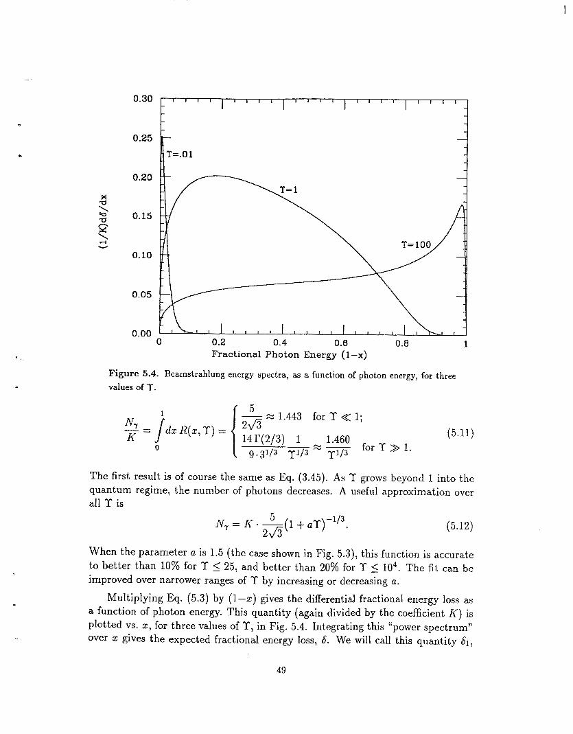
0.30

0.25

0.20

a X

d x 2

1

0.15 n

W

0.10

0.05

0.00 I l l 1 I l l 1 I I I I

0 0.2 0.4 0.6 0.8 1 Fractional Photon Energy (1 -x)

1

The first result is of course the same as Eq. (3.45). As Y grows beyond 1 into the quantum regime, the number of photons decreases. A useful approximation over all T is

-1/3 (5.12)

When the parameter a is 1.5 (the case shown in Fig. 5.3), this function is accurate to better than 10% for T 5 25, and better than 20% for T 5 lo4. The fit can be improved over narrower ranges of T by increasing or decreasing a.

Multiplying Eq. (5.3) by (l-z) gives the differential fractional energy loss as a function of photon energy. This quantity (again divided by the coefficient I ( ) is plotted VS. z, for three values of Y, in Fig. 5.4. Integrating this ‘‘power spectrum” Over X gives the expected fractional energy loss, 5. We will call this quantity 61,

49

t2 2 k

w

T

Figure 5.5. The average beamstrahlung energy loss, divided by A' = a(Az)/&,, is plotted vs. T. The dashed and dot-dashed curves show the asymptotic forms (5.13) in the classical and extreme quantum limits (to lowest order in each case). The dotted curve is the interpolating form (5.14).

since it is actually the one-photon approximation to 6, valid over distances (Az) that are small enough that the probability of emitting more than one photon is negligible. For limiting values of T, it takes the form

Palmer[1o1 has pointed out that the interpolating form

61 M - (5.14)

is remarkably accurate for all values of T. All of these approximate expressions, together with the exact formula for 61, are plotted in Fig. 5.5.

50

c

Table 2.1 lists the values of‘ 61, averaged over impact parameter assuming uniform bunches, for the SLC, NLC, and FLC. From the first quantum correction in Eq. (5.13), one can show that the quantum suppression to 61 at the SLC is about 1%. The other two values were computed by numerical integration of the function (l-z)R(s, T).

Since it is awkward to always average over impact parameter in such computations, it is tempting to introduce an “average” value of Y, from which one could evaluate 61 (and other quantities) directly. Noble‘” and others have done so, defining the average value to be some empirical coefficient times Y(edge). The danger in this practice is that the appropriate coefficient depends (weakly) on the magnitude of T, and (strongly) on what quantity one wants to compute. We will see in the next chapter, for example, that using an average value of Y to estimate the rate of coherent pair production can give grossly erroneous results. The only safe procedure is to compute averages separately in each case, from first principles, and this is what we will do throughout this paper.

The angular dependence of beamstrahlung radiation is not very interesting. As shown in Section 4.3, the radiation lies within a forward-pointing cone, centered about the electron’s local direction of travel, with opening angle N m/p in the rest frame of the positron bunch or - l / y in the CM frame. (When Y >> 1, the angle is larger by a factor of Y’1/3.) But the direction of the electron’s momentum changes by roughly this amount within one coherence length Zcoh, and the ratio L/Zcoh is typicaIly a few hundred. For all practical purposes, therefore, the opening angle of the cone is zero, and the angular dependence of the radiated photons is determined entirely by that of the radiating electrons.

5.2. Beamstrahlung from Polarized Electrons

It is well that classical synchrotron radiation has a strong linear polarization, in the direction of the electron’s acceleration. Here we will investigate the polarization of the radiation, and of the radiating electrons, in the quantum regime. Since the electrons at a future linear collider are likely to be longitudinally polarized, we use the helicity basis of polarization states.

As we saw in Section 4.4, the various terms in Eq. (5.1) correspond to the different possible helicities of the outgoing electron and photon. The first term within the brackets gives the probability for the electron to emit a photon without changing its helicity. Within the second factor of this term, the 1/2z term corresponds to emission of a photon with helicity parallel to the electron’s, while the x2/2x term corresponds to emission of a photon with opposite helicity. (This x-dependence is the same as in the Weizsacker-Williams distribution.) The second term within the brackets gives the probability for the electron to emit a photon

51

0.05

0.04

0.03

0.02

0.01

0.00

0

0 0.2 0.4 0.6 0.8 1 Fractional Photon Energy (1 -x)

Figure 5.6. The relative probability of helicity-flip beamstrahlung radiation is plotted vs. the photon energy for three values of T. As in the preceding graphs, the vertical scale is normalized to units of I<.

while flipping to the opposite helicity; in this case the photon’s helicity is always the same as the initial helicity of the electron.

The helicity-flip term of R(s, T) is plotted in Fig. 5.6, again for three different values of T. The integral of this term over x, which gives the total probability of helicity flip radiation divided by K , is plotted in Fig. 5.7. The total helicity-flip probability is negligible when T << 1, and quite small even when T X 1. At the NLC, for example, a typical electron has T M .4 and I( M 3, so the probability that it will flip its helicity by the time it leaves the bunch is about 2.5%. The average beam polarization over the entire bunch crossing is reduced by half this much, just over 1%. For the FLC the depolarization is slightly less. Furthermore, the electrons that flip tend to be those that emit very hard photons, losing most of their energy. The dilution of the polarization of the electron beam from this process is therefore unimportant for all practical purposes whenever 6 is tolerably small. One can conceive of experiments that would require better than 99% polarization:3g1 although no one has yet conceived of an electron source that could deliver anything

52

..

0.020 - I I l l " l l~ I I I 1 1 1 1 1 I I ' " l l '~ I I l 1 1 1 1 1 ~ I l 1 l 1 1 1 1 ( I I 1 1 1 1 1 1 1 I I 1 1 1 1 1 1

- - - t

T

Figure 5.7. The total probability of helicity flip beamstrahlung, divided by I<, as a

function of T.

close to 99%. Our analysis indicates that even if the machine could deliver 100% polarization, helicity-flip beamstrahlung would reduce it to roughly 99%!401

A more interesting consideration is the polarization of the emitted photons. From the s-dependence of the various terms in Eq. (5.1), we see that soft photons (with (1-3) << 1) have no longitudinal polarization, while hard photons (with (1-s) - 1) tend to have helicities parallel to the initial electron. At the FLC, for example, a typical electron (with Y = 18 and K = 2.3) emits .2 photons with (1-x) > .5, and 92% of these have parallel helicity. Figure 5.8 shows the photon spectra for Y = 1 and Y = 100, broken into parallel and anti-parallel helicity components. Thus whenever the electrons are polarized, and there is a significant hard-photon spectrum, the hard photons are polarized. Beca.use of the spin-flip term in Eq. (5.1), the polarization of hard beamstrahlung photons is somewhat greater than that of hard virtual photons (from the Weizsacker-Williams distribution). One possible use of polarized photons at a linear collider is to measure the polarization asymmetry of the reaction ey ---f Wv, in order to study the W-photon coupling!']

53

r-4 Ld 3

1 .o

0.8

0.6

0.4

0.2

0.0

Fractional Photon Energy (1-x)

Figure 5.8. Beamstrahlung photon spectra, for two values of T, broken into helicity components. The solid curves are for photons with helicity parallel to the (initial) electron, while the dashed curves are for photons with helicity antiparallel to the electron.

5.3. Multiple Photon Emission

When crL/l,,h X 1, an electron has a significant chance of emitting more than one photon before leaving the bunch. If, in addition, 61 is more than a few percent, then radiation reaction is significant: the electron’s energy loss will reduce subsequent radiation. In Section 3.4 we treated radiation reaction in the classical regime, where all the photons are very soft; now let us turn to the general case.

From Eq. ( 5 . 3 ) , we see that the probability of emitting a photon within one coherence length is -a. This implies that multiple photon emission is an incoherent process: interference between the photons can be neglected. Following Ref. 8, we will therefore apply formula (5.1) locally throughout the electron’s trajectory.

Let p be the initial energy of the electron, and suppose that at some point along its trajectory it has energy xp. It can then make a transition to energy x‘p by emitting a photon with energy (IC - x’)p . To find the probability for such a transition we substitute p --+ xp and 2 --+ x ’ / x in Eq. (5.1). Thus the probability

U

0 0.2 0.4 0.6 0 .a 1

54

per unit length is

00

T ( x I 6 x ) G - - - - cym2 I d . Ai(v) [ (F - 1) (-) X2+X’2 + (x-x‘)2 ] , (5.15) dx’dz x2p 22s’ 2x2’

U

where

(5.16)

We have defined Y = plEl/m3 in terms of the initial energy p . In general Y can still depend on z , through the electric field strength E. The coefficient m2/p is equal to l/Ylcoh, but is clearly independent of z.

Let P,(z,x)dx be the probability that at position z , the electron has energy between x and x + dx. Initially, this distribution is just a delta-function at x = 1:

Pe(O, X ) = S ( X - 1). (5.17)

As t increases, P,(z, x ) will increase due to transitions from higher energies down to x , and decrease due to transitions from x down to lower energies. More precisely, Pe evolves according to the “master equation”

where the two terms on the right-hand side represent the %ource” and “sink” of electrons at momentum fraction x . It is trivial to check that the total probability

P,(z, x)dx is conserved.

Similarly, the photon probability distribution Py(z, x ) is governed by the equa- t ion

(5.19) z

From Eqs. (5.18) and (5.19) it is easy to show that the total energy, x(Pe+Py)dx, is also conserved.

From now on we will assume that the bunch is uniform in the longitudinal direction. (We saw in Section 3.3 that this approximation introduces only a 2.3% error in the classical value of 6.) Also, as always, we will neglect disruption. Then Y is a constant for any given electron, and the kernel T(x’ + x ) is independent oi z.

55

Equation (5.18) can be solved analytically in some regimes!21 The simplest example is at x = 1, where it reduces to

(5.20)

The integral on the right-hand side is just the expected number of photons radiated per unit length, N,/L. The solution of Eq. (5.20) is therefore simply

Pe(z, 1) = Pe(O,1> e-N7z/L. (5.21)

In other words, the probability that the electron has radiated zero photons after traveling a distance z is exp(-N,z/L). The value of Nr in any particular case can be estimated from Fig. 5.3, or Eq. (5.12).

When x is very close to 1 (precisely, (1-z)/T << l), the solution is only slightly more difficult. In the source term of (5.18) we can assume z M z M 1; in this limit the kernel (5.15) becomes

/

(5.22)

The constant TO is roughly of order l/(T'/31coh). In the sink term of (5.18) we can set z equal to 1 in the limit of the integral and in ?'(x' t z), so that the integral again gives N,/L. The rate equation thus reduces to

The solution of this equation can be written abstractly as

z 1

Pe(z, x ~ l ) = e-NTz/L Jdz' eNTZ'IL /dz ' Pe(z', 2') - TO (5.24) (2' - 2)2/3

0 2

This equation can be solved by iteration, using Pe(z,x) = S ( x - l)eN7r/L as a first trial solution. The result is

The second term in brackets represents electrons that fall in energy from E to z E by radiating a single photon, while successive terms represent electrons that make the

56

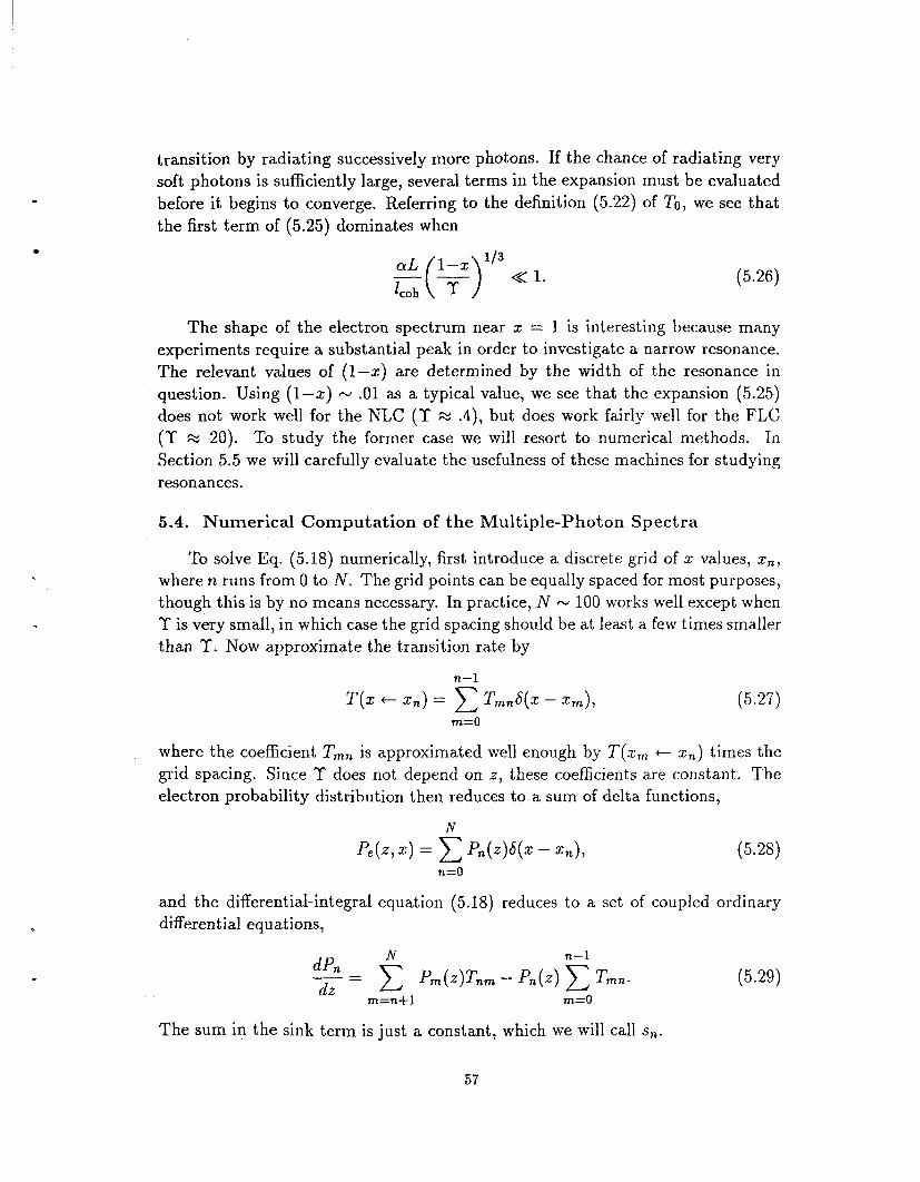
transition by radiating successively more photons. If the chance of radiating very soft photons is sufficiently large, several terms in the expansion must be evaluated before it begins to converge. Referring to the definition (5.22) of To, we see that the first term of (5.25) dominates when

(5.26)

The shape of the electron spectrum near x = 1 is interesting because many experiments require a substantial peak in order to investigate a narrow resonance. The relevant values of (1-x) are determined by the width of the resonance in question. Using (1-2) - .01 as a typical value, we see that the expansion (5.25) does not work well for the NLC (Y X .4), but does work fairly well for the FLC (T X 20). To study the former case we will resort to numerical methods. In Section 5.5 we will carefully evaluate the usefulness of these machines for studying resonances.

5.4. Numerical Computation of the Multiple-Photon Spectra

To solve Eq. (5.18) numerically, first introduce a discrete grid of x values, xn, where n runs from 0 to N . The grid points can be equally spaced for most purposes, though this is by no means necessary. In practice, N - 100 works well except when T is very small, in which case the grid spacing should be at least a few times smaller than T. Now approximate the transition rate by

(5.27)

where the coefficient Tmn is approximated well enough by ?'(xm t x n ) times the grid spacing. Since Y does not depend on z , these coefficients are constant. The electron probability distribution then reduces to a sum of delta functions,

N (5.28)

n=O

and the differential-integral equation (5.18) reduces to a set of coupled ordinary differential equations,

N n-1

m=n+l m=O

The sum in the sink term is just a constant, which we will call s,,.

(5.29)

57

n

3i ;! 1200

900

600 z/1,,,=300

2

- - - - -

1 - - - - -

0 I I I t

0 0.2 0.4 0.6 0.8 1 Fractional Electron Energy x

Figure 5.9. Evolution of the electron probability distribution, for Y = .2. In this example the bunch is taken to be unrealistically long (with a fixed field strength), to highlight the effect of radiation reaction. The peak at z = 1 is essentially gone by the time Z/ / ,& = 600.

Given the boundary conditions

p ~ ( 0 ) 1, Pn(0) = 0 for n # N , (5.30)

Starting with PN(z) and working down one by one to lower n, we can find all the solutions by direct integration.

Figure 5.9 shows the evolution of the electron probability distribution with z for Y = .2 and z / l c o h ranging up to 1200. This is in the quasi-classical regime, and the behavior is somewhat like that of the classical result (3.31). The peak of the distribution moves down in energy, but more slowly as the energy decreases.

58

.

.

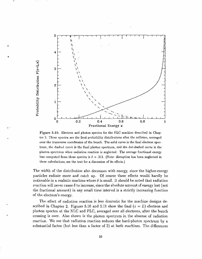
Fractional Energy x

Figure 5.10. Electron and photon spectra for the NLC machine described in Chap- ter 2. These spectra are the final probability distributions after the collision, averaged over the transverse coordinates of the bunch. The solid curve is the final electron spectrum, the dashed curve is the final photon spectrum, and the dot-dashed curve is the photon spectrum when radiation reaction is neglected. .The average fractional energy loss computed from these spectra is 5 = .211. (Note: disruption has been neglected in these calculations; see the text for a discussion of its effects.)

The width of the distribution also decreases with energy, since the higher-energy particles radiate more and catch up. Of course these effects would hardly be noticeable in a realistic machine where S is small. It should be noted that radiation reaction will never cause 5 to increase, since the absolute amount of energy lost (not the fractional amount) in any small time interval is a strictly increasing function of the electron's energy.

The effect of radiation reaction is less dramatic for the machine designs described in Chapter 2. Figures 5.10 and 5.11 show the final ( z = L ) electron and photon spectra at the NLC and FLC, averaged over all electrons, after the bunch crossing is over. Also shown is the photon spectrum in the absense of radiation reaction. We see that radiation reaction reduces the hard-phot.on spectrum by a substantial factor (but less than a factor of 2) at both machines. The differences

59

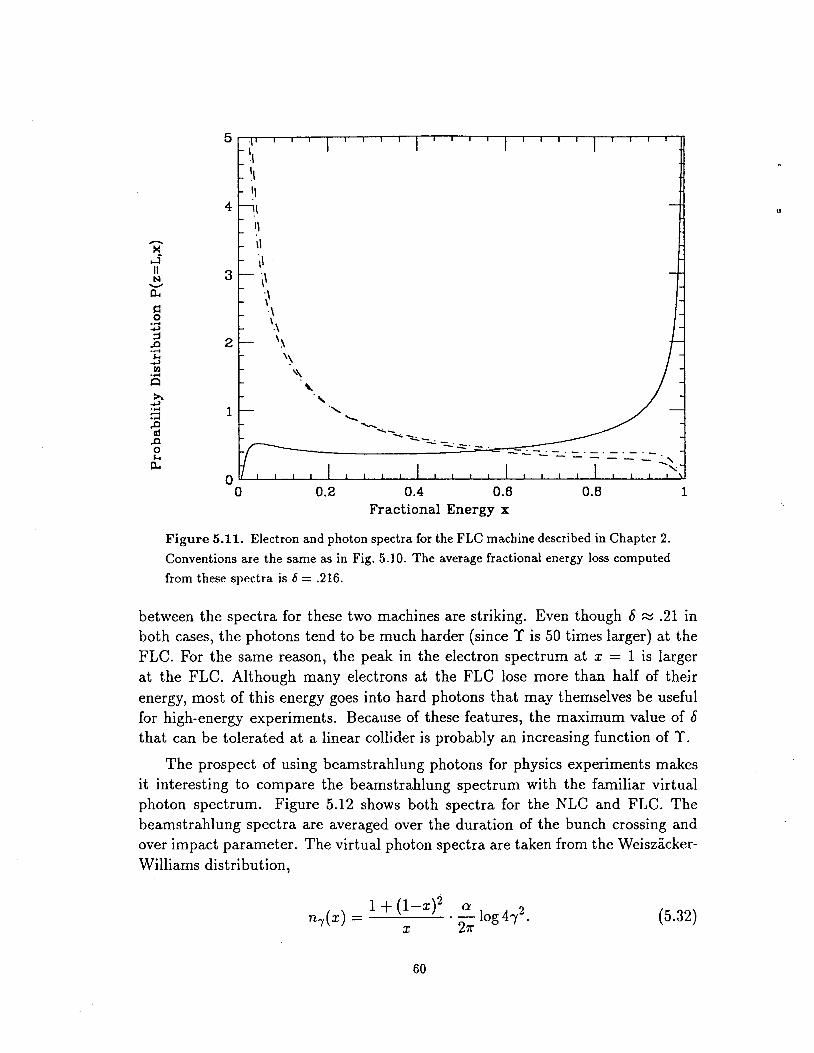
II

a W N

P P (d

0 & a

Fractional Energy x

Figure 5.11. Electron and photon spectra for the FLC machine described in Chapter 2. Conventions are the same as in Fig. 5.10. The average fractional energy loss computed from these spectra is 6 = .216.

between the spectra for these two machines are striking. Even though 6 M .21 in both cases, the photons tend to be much harder (since T is 50 times larger) at the FLC. For the same reason, the peak in the electron spectrum at x = 1 is larger at the FLC. Although many electrons at the FLC lose more than half of their energy, most of this energy goes into hard photons that may themselves be useful for high-energy experiments. Because of these features, the maximum value of S that can be tolerated at a linear collider is probably an increasing function of T.

The prospect of using beamstrahlung photons for physics experiments makes it interesting to compare the beamstrahlung spectrum with the familiar virtual photon spectrum. Figure 5.12 shows both spectra for the NLC and FLC. The beamstrahlung spectra are averaged over the duration of the bunch crossing and over impact parameter. The virtual photon spectra are taken from the Weiszacker- Williams distribution,

1 + (1-.)2 CY 4 4 = - - log 47 . 2 X 27r

(5.32)

60

2.0

1.5

1 .o

0.5

0.0 0 0.2 0.4 0.6 0.8 1

Fractional Energy x

Figure 5.12. Comparison of beamstrahlung and virtual photon spectra. The solid curves show the beamstrahlung photon spectrum, averaged over the entire bunch crossing, for the NLC and FLC. The dashed curve shows the virtual photon spectrum (from the Weiszacker-Williams distribution) for the NLC. (The virtual photon spectrum for the FLC is approximately 17% larger.) Again, disruption has been neglected in computing the beamstrahlung spectra.

This function is always larger than the beamstrahlung distribution at very large and very small x, but at the FLC both of these regimes are quite narrow and the bearnstrahlung spectrum is 2-3 times larger over a very wide range in between. At the NLC the beamstrahlung spectrum dominates from very small x up to about x = .58, above which it falls exponentially while the virtual photon spectrum remains relatively flat. [431

Going back to Figs. 5.10 and 5.11, we can compare the values of S computed from these spectra to S1, the value that we would obtain by neglecting radiation reaction. We find that S is less than 61 by about 17% for the NLC and 11% for the FLC. The values of S (denoted S,, since they are computed for uniform bunches) for both machines are listed in Table 2.1. Whether S or SI is the more appropriate quantity is not clear. The percent effect of radiation reaction on the average energy

61

throughout the bunch crossing, for instance, would be roughly half as much as on the final value of S.

Of course we have still neglected many factors in computing 6: disruption, nonuniform bunch shapes, the spread in the initial particle momenta, errors in beam alignment, and so on. To include these effects, Monte-Carlo simulation codes have been developed by Noble[” and independently by Yokoya. Since it is impractical to simulate the behavior of 1010 particles, these codes use a smaller number (lo4 for the computations described here) of “macro-particles”, which are given a proportionally larger electric charge for the purpose of computing the field strength. The macro-particles are randomly located with a gaussian distribution in all three dimensions. Whether a particle radiates a photon during a small time interval is computed randomly, according to the synchrotron radiation formula (5.1).

Yokoya’s simulation code, called ABEL (for Analysis of Beam-beam Effects in Linear colliders), has been run for the NLC and FLC parameters used in this paperF5] The resulting values of S are listed in Table 2.1 as Sg (for a gaussian bunch shape, with the disruption turned off) and Sd (with the disruption turned on). (The effect of the initial transverse momentum spread was also examined and found to be negligible.)

[17,441

When disruption is turned off, we find for both the NLC and FLC that 6, is roughly 20% larger than 5,. This difference is almost certainly due to the transverse gaussian bunch shape. The simulations define S as the average energy loss per particle, neglecting the likelihood that the particle will participate in a collision (when transverse momenta are present, it would be extremely difficult to define or compute a properly weighted 6). But we saw in Section 3.3 that with this definition, even the classical value of S comes out 15% larger for a gaussian bunch than for a uniform bunch.

When disruption is turned on, there is no significant change in the value of S for the FLC. For the NLC, however, 5 increases by another 35%, to the alarming value of .35. The natural explanation for this increase is the higher average field strength in the presence of horizontal disruption. For the FLC this effect is negligible, since D, = .07. But for the NLC design used here, with its unusually small aspect ratio and reasonably large value of D,, the horizontal disruption parameter is D, = .74. According to Eq. (3.6), the average horizontal beam dimension is therefore reduced by roughly 11%. The average field strength increases proportionally, as do the parameters T and l/lcoh, which are proportional to the field strength. The expected value of 6, according to Eq. (5.1) and Fig. 46, depends linearly on l/lcoh but less strongly on Y; combining the effects we would expect roughly a 14% increase in 6 from an 11% decrease in CT,. Thus we can account for nearly half of the 35%

e

62

disruption effect in the simulation, but not all. The reason for the remaining difference (or the error in the preceding analysis) is not known.

Because the effect of horizontal disruption is not well understood, it has been completely neglected in the rest of this paper, except in its effect on the pinch enhancement H D (which is much larger for the NLC than for any machine with very flat bunches) and thus on the luminosity. This inconsistency is hardly fair, since the plots in this chapter could easily give the impression that the beamstrahlung energy loss at the NLC is much smaller than it actually is. These plots are unquestionably wrong; the only uncertainty is over how much. This issue requires careful investigation before machine designs in this parameter regime can be properly evaluated.

There still remains the question of how to best define 6. We have seen in this section that radiation reaction reduces S by 17% at the NLC, but the effect #of this reduction on the average available collision energy will be smaller. We have also seen that there is no obviously correct definition of 5 when the bunch is nonuniform. Both of these ambiguities are avoided if we discuss only the spectra of CM energies at which actual collisions between particles occur. We now turn to the computation of these spectra.

5.5. Luminosity Spectra

In Section 3.6 we saw that the luminosity spectrum in the classical case can be crudely approximated with very little effort. In the quantum case, however, the probabilistic nature of the radiation requires us to treat the computation more properly.

First imagine a collision between two relativistic particles with well-defined energies z l E and z2E. Let E,-, = 2E be the “nominal” center-of-mass energy, and ecm the total energy in the true center of mass. The ratio ecm/Ecm is then

(5.33)

Next let the energies of these particles be distributed according to probability distributions Pl(x1) and P2(z2). Then the differential luminosity as a function of X is given by

1 I

0 0

(5.34)

This distribution is normalized to 1 provided that PI and P2 are normalized to 1.

63

A

Figure 5.13. One moment during the bunch crossing, and one point at which to evaluate the contribution to the luminosity spectrum.

Now consider the situation depicted in Fig. 5.13, and concentrate on collisions occurring at point A. Electrons located at a distance z 1 behind the front of the electron bunch are colliding with positrons located at a distance z2 behind the front of the positron bunch. Since the electrons have passed through a length 2 2 of the positron bunch, their probability distribution PI should be evaluated at z = 2 2 ;

conversely, the positron probability distribution P 2 should be evaluated at 2 1 . The luminosity spectrum coming from this instant is therefore

Finally we must integrate over all places and times in the entire bunch crossing. Since the electron encounters positrons throughout the length of the positron bunch, we must average over values of 22 from 0 to 1. And since the electron could have been at any point zl within the electron bunch, we must also average over values of z1 from 0 to 1. The luminosity spectrum for the entire bunch crossing (but still for a single impact parameter) is therefore

64

The integrals over z1 and z2 are most easily performed first. Defining

. L

L - P ( x ) = I” L P(z , x),

0

we have simply

1 1

(5.37)

- d X dC = /dxl /dx2P1(21)Tii2(12)s(X - =)- (5.38) 0 0

Using the delta function to perform the x2 integral, we obtain the less symmetrical but more useful formula

dC 2x - dX (5.39)

Either (or both) of the distributions PI and P2 appearing in the above formulae could be for photons rather than electrons or positrons. Thus we can compute the luminosity spectra for e+e-, ey, and yy collisions. All three spectra, computed numerically from the probability distributions of the previous section, are shown for the NLC in Fig. 5.14 and for the FLC in Fig. 5.15. Here we have averaged over impact parameter, assuming a uniform elliptical bunch shape. The dependence of the spectra on the transverse bunch shape is shown in Fig 5.16, which compares the NLC spectra of Fig. 5.14 to the corresponding spectra for a gaussian bunch shape. The difference is negligible for most purposes. (For simplicity, the field strengths used to compute the curves in Fig. 5.16 are actually for a round bunch, with or chosen so that the corresponding round uniform bunch has the same field strengths inside as the elliptical uniform bunch. In any situation where these tiny differences might matter, one should compute the spectra properly for a flat bunch with a gaussian profile in all three directions. Of course by the time the bunches at a linear collider reach the interaction point, they are probably no longer gaussian anyway.)

Notice from Figs. 5.14 and 5.15 that while the luminosities at large X for e y and 77 collisions are non-negligible, they are still quite a bit smaller than the e+e- luminosity. It should be emphasized, however, that the parameters of these machines were chosen under the assumption that a larger beamstrahlung energy loss could not be tolerated. Higher photon luminosities could certainly be obtained

65

X = Fractional C.M. Energy

Figure 5.14. Luminosity spectra for the NLC parameters given in Table 2.1. The solid curve is for electron-positron collisions, the dashed curve is for electron-photon or positron-photon collisions (either separately-not the sum of both), and the dot-dashed curve is for photon-photon collisions. The spectra are averaged over the duration of the bunch crossing (assuming a uniform longitudinal bunch profile) and over the transverse coordinates (assuming a uniform elliptical cross-section), neglecting disruption. See the end of Section 5.4 for a discussion of the effects of disruption.

if desired, by redesigning the machines or (to a lesser extent) by changing the final- focus optics to obtain a smaller aspect ratio. As was first pointed out in Ref. 8, the prospect of using beamstrahlung photons for physics experiments should be seriously considered in the design of a linear collider.

As discussed at the end of Section 5.3, it is important to know what fraction of the luminosity of a collider is within a small range of the maximum CM energy. We are now in a position to answer this question. Define l ( X ) to be the fraction of the luminosity at a fractional CM energy greater than or equal to X. First let us calculate t(l), the luminosity that is exactly at the CM energy, which comes from electrons that have not radiated at all. Inserting the delta function term (5.21) of the probability distribution into Eq. (5.38), we find

66

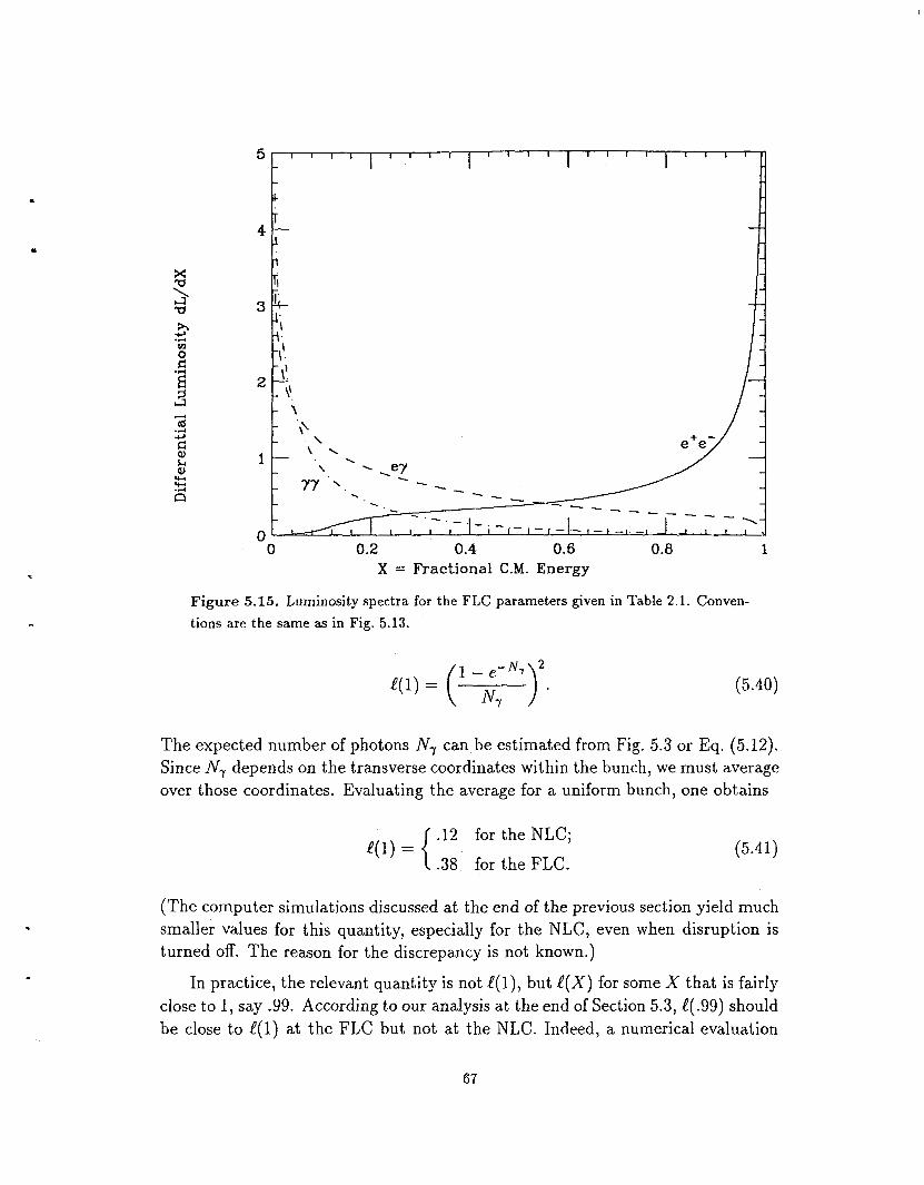
. U

c X = Fractional C.M. Energy

Figure 5.15. Luminosity spectra for the FLC parameters given in Table 2.1. Conven- tions are the same as in Fig. 5.13.

(5.40)

The expected number of photons N, can be estimated from Fig. 5.3 or Eq. (5.12). Since N-, depends on the transverse coordinates within the bunch, we must average over those coordinates. Evaluating the average for a uniform bunch, one obtains

.12 for the NLC; -38 for the FLC.

!(l) = (5.41)

(The computer simulations discussed at the end of the previous section yield much smaller values for this quantity, especially for the NLC, even when disruption is turned off. The reason for the discrepancy is not known.)

In practice, the relevant quantity is not '(l), but ' ( X ) for some X that is fairly close to 1, say .99. According to our analysis at the end of Section 5.3, -e( .99) should be close to e( 1) at the FLC but not at the NLC. Indeed, a numerical evaluation

67

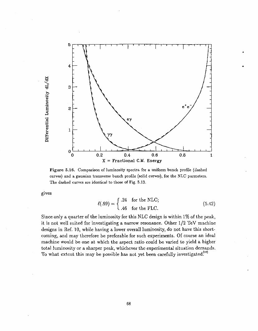
4 R .i

0 m

0 0.2 0.4 0.6 0.8 1 X = Fractional C.M. Energy

Figure 5.16. Comparison of luminosity spectra for a uniform bunch profile (dashed curves) and a gaussian transverse bunch profile (solid curves), for the NLC parmeters. The dashed curves are identical to those of Fig. 5.13.

gives .24 for the NLC;

iY.99) = \ I I .46 for the FLC.

(5.42)

Since only a quarter of the luminosity for this NLC design is within 1% of the peak, it is not well suited for investigating a narrow resonance. Other 1/2 TeV machine designs in Ref. 10, while having a lower overall luminosity, do not have this short- coming, and may therefore be preferable for such experiments. Of course an ideal machine would be one at which the aspect ratio could be varied to yield a higher total luminosity or a sharper peak, whichever the experimental situation demands. To what extent this may be possible has not yet been carefully investigated!"]

68

6. Coherent Pair Production

Coherent pair production is the inverse of beamstrahlung: a photon, in the presence of a strong electromagnetic field, converts to an electron-positron pair. The process is illustrated in Fig. 6.1.

e-

e +

Figure 6.1. Feynman diagram for coherent pair production.

The rate of this process is simply related to that of beamstrahlung by the crossing relations

Let us make the following definitions:

where

x2 + (1 -x)2 2x( 1-x) ) + 2x(l-x)

U

69

( l - ~ ) ~ ) 21 Ai'(u) + r d v Ai(v)]. x( 1 -x)

U

Note the close resemblance to the synchrotron radiation formulae (5.1) and (5.6). The precise correspondence under the crossing relations (6.1) is explained fully in Refs. 29 and 14.

The history of Eq. (6.3) is almost identical to that of the synchrotron radiation formula (5.1). The first full treatment of the problem, using explicit wavefunctions in a uniform magnetic field, was given by Klepikov:'' while our relatively simple form of the result is due to Nikishov and Ritus?] Baier and Katk~v" '~ later obtained the same result by more abstract methods; a nice treatment from their viewpoint can be found in the textbook of Berestetski, Lifshitz, and Pitaevskii?' Most recently, the formula has been derived using scattering-theory formalism (similar to that of Chapter 4 of this dissertation) by Blankenbecler, Drell, and Kroll!"] The importance of this process in beam-beam interactions was first recognized by Chenfl2] and has been discussed in more detail by Chen and Telnov. [13.46j

The implications of Eq. (6.3)) however, are quite different from those of the synchrotron radiation formulae. The pair production spectra for several values of Yk are plotted in Fig. 6.2. The most striking features are the symmetry under x + (1-x), the exponential suppression as either x or (1-2) goes to zero, and the exponential suppression in the total rate when Yk < 1.

To verify the exponential suppression, note that the new u , defined in Eq. (6.2)) grows large compared to 1 whenever x, (1-x), or Yk is small. In any of these three circumstances we can use the asymptotic expansion (5.8) of the Airy function to obtain

The conditions for this suppression to occur can be stated more directly if we define

these are just the usual quantity Y, evaluated for the momenta of the outgoing electron and positron. The exponential suppression of the pair production rate occurs when either T- or Y+ is small compared to 1. In other words, very soft particles are never produced by this process. To emphasize this fact, Fig. 6.3 shows an expanded view of the soft end of the spectrum for the same values of Tk as in Fig. 6.2.

70

0.15

0.10

0.05

1

0.2 0.4 0.6 Fractional Energy x

0.8 1

Figure 6.2. Coherent pair production spectra for several values of Tk.

When Tk << 1, the spectrum is strongly dominated by the region near x = 1/2. Expanding about this point and integrating over x, we obtain the total probabilityYg1

dP

Coherent pair production is therefore completely negligible when T << 1. For example, even if there were one very hard photon for each electron in the bunch, less than one coherent pair would be produced per bunch crossing when T < .l. We will make some more careful estimates below, taking the beamstrahlung photon spectrum into account.

When both T- and T+ are of order 1, the pair production rate is comparable to the synchrotron radiation rate for the same field strength; that is, the probability of pair creation within one coherence length is of order 1/a. When both T- and T+ are much greater than 1, we can set u = 0 wherever possible in Eq. (6.4) to obtain

71

100

10-1

10-2

10-3

10-4

10-5

10-6 0 0.01 0.02 0.03 0.04 0.05

Fractional Energy x

Figure 6.3. Expanded view of the leftmost 5% of Fig. 6.2. No matter how large Tk is, the spectrum is exponentially suppressed when T- = z T ~ << 1.

Although this expression is never valid when x or (1-2) is very small, we can still integrate it over x from 0 to 1 to obtain the asymptotic total rate in the Tk >> 1 limit PSI.

The rate falls off as T-’I3, just as it does for synchrotron radiation. Figure 6.4 shows the total pair production rate over a wide range of Ti;.

Coherent Pairs from Beamstrahlung Photons

So far all of the expressions in this chapter are for the number of pairs created per photon. In the beam-beam interaction, however, the photons are created continually a t a rate determined by the synchrotron radiation formula (5.1). To estimate the number of pairs, therefore, we should fold the pair production rate with the beamstrahlung spectrum.

As in the previous chapter, let us consider the idealized situation in which the bunch is uniform in the longitudinal direction and the disruption is very small.

72

w 0

Tk

Figure 6.4. The total probability of coherent pair production, divided by the coefficient a(Az)/l, ,h, is plotted vs. Th. The dashed curve shows the limitingform (6.7) for Tk << 1, and the dot-dashed curve shows the limiting form (6.9) for Tk >> 1.

Then the electric field along any given electron’s trajectory is consant, so Y and lcoh are constant. Finally, let us neglect radiation reaction; this will cause us to over-estimate the number of hard photons, and hence the number of coherent pairs, by several percent in most cases. With all these simplifications, the spectrum of pairs produced by a single incident electron is obtained simply by folding the pair production rate (6.3) with the beamstrahlung spectrum (5.3). If x represents the fractional energy of one member of the pair, as a fraction of the energy of the incident electron, then the differential probability is

L l d P - = /dz /dy --S(x/y,yT) - Z R ( l - y , Y)

a 1 dx lcoh Y lcoh

o z

(6.10)

Here S is the pair production spectral function (6.4), R is the beamstrahlung

73

0.08

0.06

h 2 n P 0.04

,-I .d

td

0 k a a 3

0) 0.02 5 n

k

0.00 0 0.2 0.4 0.6 0.8 1

Fractional Energy x

Figure 6.5. Coherent pair production spectra, taking the beamstrahlung photon spectra into account, for three values of Y. The curves were computed by numerical integration of Eq. (6.10), divided by the normalization constant K2, where I< = crL/l,,h. The curve for Y = 1 has been multiplied by 10 for clarity.

spectral function (5.4), and y is the fractional energy of the intermediate photon. The factor of l / y arises from the fact that Eq. (6.10) is differential in x, rather than x/y. The total probability of pair production by this electron can be found by integrating over x:

0 0

The inner integral is just the function plotted in Fig. 6.4, proportional to the total probability of pair creation by a single photon with fractional energy y.

For a more accurate treatment of the beamstrahlung photon spectrum, one can use the rate equations (5.18) of Section 5.3. It is straightforward to a source term to the electron master equation representing pair production. Similarly, the photon equation would now have a pair-production sink and a second source, from the positrons. Finally, there is now a third equation, identical in form to' the

"

.

electron equation, for the evolution of the positron spectrum. The rate equations can be solved numerically as in Section 5.4. We will not do so here, however, since accuracy of this order is not necessary for our purposes. For the NLC in particular, inaccuracies due to assumptions about the bunch geometry are much more significant, as we will see in Section 7.2.

Equations (6.10) and (6.11) simplify considerably in the limit Y << 1. Inserting the approximate expressions (5.9) for R'and (6.5) for S, we find that the differential probability (6.10) has an exponential suppression factor of the form

1 - d P M Jdy (e-.) e x p [ - L ( z + dx 3T 1-y x(y-x)

2

(6.12)

The exponent has a maximum at y = (l+x)/2. Expanding about this point, we obtain the asymptotic form

(This formula is accurate to within several percent up to T = 1.) To find the total number of coherent pairs in this limit we integrate over x, expanding about the maximum of the exponent (which occurs at x = 1/3). The result is

(6.14)

(This result can also be obtained by plugging Eq. (6.7) into (6.11) and then integrating over y.) Notice the very strong dependence on T in this formula: a 13% error in the value of Y would change the result by a factor of 2.

Of perhaps more interest is the form of the spectrum (6.13) when x << 1 (that is, when one member of the pair is very soft). Setting z = 0 wherever possible, we obtain simply

(6.15) We are generally interested in machines for which T > .1 and crL/Zcoh - 1. For order-of-magnitude estimates in these cases we can use the expression

- dP -2/(3Tz) - - e (6.16)

(This is the same expression we would have obtained directly from Eq. (6.5), neglecting the photon spectrum.) The total probability of creating a pair with x < x0

dx fi

is given by the integral of d P / d x , which in this case is roughly

(6.17)

When Y = 1 and zo = .03, for example, the total probability is of order We will make more numerical estimates in the next chapter.

Angular Distribution of Coherent Pairs The angular distribution of coherent pairs is no more interesting than that of

beamstrahlung photons. The electron and positron come out at an initial angle of order rn/kr7’ which is roughly 100 times smaller than the typical angle of the initial photon (which it inherited from its parent electron). The pairs can, however, acquire a much larger angle as they exit the bunch, especially if their energies are much lower than that of the beam electrons. We will return to this subject in the next chapter .

76

7. QED Backgrounds at the Next Linear Collider

In the preceding chapters we have seen that the combination of high energy and high luminosity per bunch at linear colliders gives rise to several important beam- beam effects: disruption, beamstrahlung, and coherent pair production. Another important process is incoherent pair production, in which an electron-positron pair is produced in a direct collision of two photons, either real (from beamstrahlung) or virtual (emitted by a passing electron or po~itron)!‘~]

P a h c r e a t e d by the incoherent processes tend to be very soft, simply because the cross-section for 77 ---f e+e- falls off like l/E&,. In the Chl frame of the two photons, the cross-section is not strongly peaked in the forward direction. Fur- thermore, these soft pairs are disrupted very strongly by the field of the oncoming bunch, with one member of the pair always being pushed outward. If too many charged particles enter the detector during each bunch crossing, much of the detector is rendered useless. The energy spectra and angular distributions of these processes therefore merit careful investigation.

Because of the large number of processes and the wide range of energies and angles that must be considered, this subject does not lend itself to a simple, general, and accurate analytic treatment. We will therefore sacrifice accuracy and generality in favor of simplicity. We will confine our attention to the “next linear collider”, a machine with an energy of 1/2 TeV. For specific numerical examples we will use the NLC parameters in Chapter 2, always bearing in mind that other NLC designs tend to have lower luminosity and fewer (and softer) beamstrahlung photons. (A 1 TeV machine, on the other hand, would have a slightly higher luminosity and slightly harder photons.) Furthermore, we will make no attempt to compute the rates of these processes to better than a factor of 2.

7.1. Outgoing Angles and Interact ion Region Geometry

Before launching into computations of pair production rates, let us ask what the detector can tolerate. One tenta.tive proposal[4g1 for the interaction region geometry is shown in Figs. 7.1 and 7.2. In this design, the final focusing quadrupole magnet is 1 meter from the interaction point, and has a pole tip aperture of about 1 mm. The beams cross at an angle of 6 millira.dia.ns, and the outgoing beam leaves through a larger hole to the side of the quadrupole tips. (Some designs have a crossing angle as large as 50 mrad, which allows for a much larger exit hole.) Surrounding the final quadrupole and extending down toward the interaction point is a conical tungsten mask, designed to shield the detector from any radiation that might originate in the vicinity of the quadrupole.

77

Figure 7.1. A very tentative sketch of the interaction region of the next linear collider. The vertical dimension is exaggerated.

hole

Figure 7.2. A face-on view of the final focusing quadrupole. In this design the crossing angle, and therefore the exit hole, are relatively small.

78

I

.

In Section 3.1 we saw that the trajectory of a beam electron within a uniform, cylindrical, undisrupted bunch a f positrons is

Here all quantities are evaluated in the rest frame of the positron bunch. From this we can find the maximum disruption angle of an electron with the full beam energy, attained when the electron enters at the edge of the bunch and exits as it crosses the axis. The maximum disruption angle in the vertical direction, evaluated in the CM frame, is

(Here and throughout this chapter we will write expressions in terms of uz, oy) and oz) although most of the derivations are for uniform cylindrical bunches. Wherever possible, expressions are simplified by assuming o, >> uy. Numbers for the “NLC” are for the parameters given in Ta.ble 2.1.) By the same argument, the maximum horizontal disruption angle is

(Notice that this expression is independent of 6% and oY.) Since D, is generally less than I, however, the bunch crossing is over before this angle is ever attained. For our NLC parameters, D, equals .74, so the actual maximum horizontal angle is a.bout 1.0 mrad. For designs with a larger aspect ratio the actual angle would be still smaller. In any case, we see that an exit hole with radius 2-3 mm at a distance of 1 m from the interaction point, as in Fig. 7.2, is large enough to accept all disrupted electrons that still carry the full beam energy.

An electron that has less than the fuIl beam energy will also oscillate within the positron bunch, but with a shorter wavelength and therefore a larger maximum angle. If the electron carries a fraction z of the beam energy, its effective disruption parameter is increased by a factor of l/s, and hence the maximum outgoing angles are increased by 1/fi. Equations (7.2) and ( i . 3 ) therefore become

4Nreay 2 8 mrad 8; = - - & for the NLC; (7.4)

79

1.4 mrad 6 5 = - -

& for the NLC. (7.5)

For example, an electron with x = .01 at the NLC could acquire a vertical angle of up to 2.8 mrad, and a horizontal angle of up to 14 mrad. (If the aspect ratio o,/oy were larger, the vertical angle would be smaller but the horizontal angle would be the same.) For the design shown in Fig. 7.2, such an electron would have a good chance of hitting the face of the final quadrupole. It would then create an electromagnetic shower, with some of the resulting photons (and possibly electrons and positrons) heading back toward the interaction point. In this particular case the problem could be avoided by using a larger crossing angle and larger exit hole.

Next consider the trajectory of a positron with fractional energy x traveling in the wrong direction-against the oncoming positron beamp] It will quickly get pushed up or down to the edge of the beam, beyond which the field is very strong and relatively constant out to a distance of - Bx = 2uZ:

4 N a IE(outside)) e -

LBX for y ;S B,.

If its energy is relatively large, it will rexh the end of the bunch before leaving this strong-field region. The condition for this to occur is

where z is the distance traveled by positron from its creation until it reaches the end of the bunch. When this condition is met, the positron’s final angle is

Note that for our NLC parameters, with DX = .74, condition (7.7) is met only for fairly hard positrons.

When condition (7.7) is not met, the positron leaves the strong-field region before reaching the end of the bunch. Outside of this region the field falls off more quickly, so any additional angle it acquires will be relatively small. The angle it acquires while in the strong field is

Several comments about this formula are in order. First, it was derived under the very crude approximation of cutting off the field at a height of 2a, above the bunch;

80

since the machine design may depend on the precise coefficient in this formula, it should be checked against the more realistic situation of a gaussian bunch with the field extending to infinity. Second, the formula depends only on the positron energy 732 and the linear charge density N / a z , and is independent of a, and a,; it is therefore relatively independent of the particular machine design. Finally, it is almost identical to expression (7.5) for the maximum horizontal angle of a trapped electron oscillating within the positron bunch. This is no accident, since both results depend only on the potential difference from the center of the bunch to far outside. Aside from the factor of a, the main difference between Eqs. (7.5) and (7.9) is that only a small fraction of the trapped electrons exit with such a large angle, whereas almost every soft positron is pushed out to the same angle (7.9):’’

According to Eq. (7.9), sufficiently soft positrons can leave the interaction point at very large angles. Referring to Fig. 7.1, we see that many will hit the face of the final quadrupole and the luminosity monitor. The masking must be sufficient to block the showers from these particles almost completely. On the other hand, very soft positrons (at the NLC, with x =S 4 X or an energy of 100 MeV) will have an angle greater than 100 mrad, and will therefore hit the outside of the masking. These also create showers, with the backward-moving photons from these showers going straight into the drift chamber of the detector. A fraction of the photons then Compton-scatter off the gas in the drift chamber, and the resulting free electrons (if there are too many of them) flood the chamber with tracks. Preliminary computations with the EGS Monte-Carlo code indicate (with a very large factor of uncertainty) that for every thousand 50-MeV electrons or positrons that hit the outside of the masking at an angle of loo, a few hundred electrons are found in the drift cha.~nber!~~’

A final complication (but a welcome one) is the solenoidal magnetic field of the detector. The radius of curvature of a. charged particle with transverse momentum pT in a constant magnetic field B is (in SI units)

PT r = -. e B (7.10)

For the design of Fig. 7.1, any particle with a radius of curvature less than 1.5 cm will curl so tightly that it enters the opening in the masking, regardless of its initial angle. Let us assume the typical value of 1 Tesla for the field strength; the critical value of p , is then 4.5 MeV. Returning to Eq. (7.9), we find that for low-energy positrons,

p , = f i . 500 hleV for the NLC, (7.11)

and therefore that positrons with x < 8 x low5 will enter the opening in the masking. A more careful analysis, taking the precise trajectory into account, raises

81

this limit very slightly, to 9.3 X and also lowers the limit of the preceding paragraph from 4 x low4 to 3.7 x

The conclusion from this analysis is that for a 1/2 TeV collider with N/ut as in the NLC design of Table 2.1, an interaction region geometry as in Fig. 7.1, and a solenoidal field strength of 1 T, there exists a small but significant range of energies for which a positron traveling in the wrong direction is pushed out to a large angle and hits the outside of the masking. That range is roughly

9 X < x < 4 X or 25 MeV < E < 100 MeV. (7.12)

High-energy positrons, above the upper limit, acquire too small an angle as they exit the bunch, while low-energy positrons, below the lower limit, are contained in the solenoidal field. The upper limit could be reduced by increasing the angle of the conical masking, while the lower limit could be raised by increasing the solenoidal field strength'531 or increasing the dia.meter of the opening in the masking. The disadvantage of the latter approach is that the masking must shield the detector from photons created by high-energy positrons (and electrons) hitting the face of the quadrupole magnet, as well as from showers initiated by synchrotron radiation emitted by the beam as it is bent by the quadrupoles. Monte Carlo simulations to study the effectiveness of various ma.sking designs are currently underway.

The analysis of outgoing angles i n this section has neglected any intrinsic angle that an electron or positron might have when it is initially created. As we will see below, a small fraction of the pa.irs created by the incoherent processes have angles that are comparable to, or larger than, the acquired angle (7.9). In this case Eq. (7.12) no longer applies, and any electron or positron with

e > 100 mrad a.nd p , > 4.5 MeV (7.13)

is potentially dangerous. Again, however, these limits are sensitive to the geometry of the masking and the solenoidal field strength.

7.2. Coherent Pair Production

We saw in the previous chapter t11a.t i n the NLC regime where T 6 1, the coherent pair production rate depends exponentially on Y'. This process is therefore completely dominated by the region of space and time during the collision where the field strength attains its highest value, while the number of coherent pairs is extremely sensitive to the magnitude of this value. Because of this sensitivity, we will estimate only orders of magnitude in this section. A more accurate analysis would require a careful trea.tment of the precise bunch geometry, including the effects of disruption.

The value of Y(edge) for the NLC in Table 2.1 is .56; this is the value of T at the edge of a uniform cylindricd bunch. When the bunch has a transverse gaussian profile, the maximum value of Y is slightly (and negligibly) less. A gaussian shape in the longitudinal direction, however, has a large effect. We saw in Eq. (4.90) that the maximum field strength in this case is larger than that of a uniform bunch by a factor of m. Another significant effect for this NLC design is horizontal pinching (since D, = .74 is relatively large), which increases the average field strength by about lo%, and increases the maximum field strength by much more. The maximum field with pinching, however, is only felt by the tail of the oncoming bunch. For our present order-of-magnitude estimate, therefore, let us use the average value of 10%. Our estimate for the maximum value of Y is therefore

Ymax = .56 m 1 . 9 = .SG for the NLC. (7.14)

To compute the total number of coherent pairs we can use Eq. (6.14). In the coefficient f fL/&h, we should set L ecpal to the length over which the exponent exp( -16/3Y) is reasonably close to its maximum value, say within a factor of 2 (or a field strength within 13%); this length is roughly .3 times the bunch length. The coherence length lcoh is enhanced by the same factors as T, relative to its maximum value in a uniform bunch. Combining all the factors, we find

CYL -- - 1.3 for the NLC. k o h

(7.15)

We can now evaluate Eq. (6.14) to obta.in the total probability for coherent pair creation,

P x 6 x (7.16)

Slightly less than a third of the electrons pass through the region in which the field comes within 13% of its maximum value, so the total number of pairs per bunch crossing is roughly N / 3 times this number:

Number of pairs M 3 x lo5 per bunch (7.17)

M 3 x 10' per bunch train. \ I

(These numbers are for pairs going i n only one direction.) It must be emphasized that this result is uncertain by at least a factor of 2.

The spectrum of these pairs is approximated closely enough by the curve for Y = 1 in Fig. 6.5. The peak occurs near x = .3 (or E = 75 GeV), with the rate dropping much lower below z = .l. According to Eq. (7.S), the angle acquired by

83

+

Y

e -

e+

Figure 7.3. Feynman diagrams for the Breit-Wheeler process, yy -+ e+e-.

these positrons exceeds 3 mrad when x 5 .2; thus a large fraction of them would hit the face of the quadrupole in Fig. 7.2. Whether this is a problem depends on the effectiveness of the masking. If it is not tolerable, then this machine requres a larger exit hole, and therefore a larger crossing angle (as the design indeed has in Ref. 10).

The good news, as we already saw in Eq. (6.17), is that none of the coherent pairs (that is, less than one per bunch train) have 2 < .03. According to Eq. (7.9), this implies that none acquire an angle larger than 12 mrad. With a crossing angle of 50 mrad it should be easy to make the exit hole large enough to accept every positron produced in this process. None of them come anywhere close to the 100 mrad angle of the masking.

If a small crossing angle is required for other reasons, and the masking is not sufficient to block the showers from lo6 high-energy positrons hitting the quadrupole face, then one is forced to consider NLC designs with smaller values of T. As an example at the other extreme, machine F in Ref. 10 has Tmax M .22, and therefore, according to Eq. (6.14), less than one coherent pair produced per bunch train. Thus it is certainly possible, one way or another, to avoid all background problems from coherent pair production.

7.3. The Breit-Wheeler Process, y y + e+e-

The simplest incoherent pair production process is the direct collision of two real photons to create an electron-positron pair. This is just a cross-channel of Compton scattering; the two leading-order Feynman diagrams are shown in Fig. 7.3.

The cross-section for this process is easy to compute, and even easier to find

84

in standard textbooks!'' The total cross-section is

asw=?rr?(1-P2)[?83-4P+(3-P4)log(=)], 2 1 - P (7.18)

where P is the velocity if the electron (or positron) in the CM frame of the two colliding photons. In the limit where ,8 --+ 1, this becomes

(7.19)

where w is the energy of each of the photons in the CM frame. In a general frame where the photon energies are ul and w2, replace w2 -+ wlw2.

To calculate the number of pairs produced by this process we must fold the cross-section with the beamstrahlung photon spectrum. Since the cross-section is largest for soft photons, we can use the soft-photon approximation (5.7), divided by 2 to average over the bunch length:

aL - Ai'(0) ny(x) = ( I > coh 'r1/3x2/3 (7.20)

Here x = w / E is the fractional energy carried by the photon. The quantities T and [,-oh depend, of course, on the coordina.tes (b , s ) within the bunch. Let us assume a uniform cylindrical bunch geometry. Then the total number of Breit-Wheeler pairs created per bunch crossing is

NBw = / d 2 b N 2 H D

( 4 7 r W J 2 (7.21)

The integral over b cancels one factor of 47ra,ay and gives 3/5 times the integrand evaluated at the edge of the bunch. It is convenient to evaluate the coefficient of the photon spectrum at the edge once and for all:

(7.22)

This coefficient is proportional to IEl(edge)13/3, and is therefore much smaller for machine designs with a larger aspect ratio aZ/ay.

The integrals over 2 1 and x2 in Eq. (7.21) are not as hard as they look. Since the total cross section depends only on the Lorentz-invariant product 2 1 2 2 , it is

natural to change the variable of the inner integral from x2 to the photon energy in the CM frame, 5 E f i . ‘The expression then becomes

1 1

NBw = - / $ / dz --$ - 4P + (3 - p4) log (s)] , (7.23) r2 1 - P

where

3 N?H& KT;

5 4KcT,lYy 2 I(Bw E - - = 8.9 x lo5 for the NLC (7.24)

and y = E / m is the boost factor of the beam electrons. The integral over x is strongly dominated by the region from 1 to a few times l /y; this means that nearly all of the pairs are created near threshold in the CM frame of the colliding photons. Numerical evaluation of this integral gives 3.1 -y4/3. The value of 21 determines the overall boost of the center of mass, and therefore of the created pair. Evaluating this integral gives a factor of logy’, yielding the total number of Breit-Wheeler pairs per bunch crossing,

6.2 K B W log y’ N E W =

?213 = 2.3 x lo4 for the NLC. (7.25)

Alternatively, we can leave the integral over 21 undone to obtain the differential distribution

(7.26)

As long as x1 is not too close to l /y , we can interpret it as the fractional energy of either member of the created pair. Integrating over the dangerous range (7.12), we find that for the geometry shown in Fig. 7.1 and a solenoidal field of 1 T, approximately 1300 electrons hit the outside of the masking on one side, and 1300 positrons hit the outside of the masking on the other. (These numbers are per bunch crossing; multiply by 10 for the number per bunch train.)

Now let us consider the regime where the center of mass of the two photons is not boosted by a large amount in the lab frame. In this case the outgoing angles of the electron and positron can be large (even without the additional push from the field of the bunch). We must therefore consider the angular dependence of the fundamental yy + e+e- process.

86

The differential cross-section for 77 + e+e- is

. (7.27)

(Here we ignore the threshold behavior, since we are interested in particles that are produced with a transverse momentum of at least a few MeV.) For an asymmetric collision between photons with energies x l E and x 2 E , it is more convenient to write the cross-section in terms of the transverse momentum, p , = w sine,,:

Folding this expression with the photon spectra (7.20), multiplying by the luminosity per bunch, a.nd averaging over the transverse coordinates, we obtain

In a more exact analyis, we would now"e1iminate one of the x's in favor of the electron's or positron's a.ngle in the 1a.b frame. We would then specify a minumum value of this angle and a minimum value of p , (or the energy) and integrate up from there to count the number of troublesome pairs. For a fixed angle, however, the rate will be dominated by values of p , only slightly above our imposed cutoff (since the rate falls off very strongly with energy). We will therefore integrate directly over x1 and 2 2 , estimating the range of integration only roughly. In this approximation we can perform the p , integral immediately, throwing away all the p , dependence except the dependence on our cutoff, p;. The integral is then easy to evaluate:

Eq. (7.23)) and then to y , we obtain for the total number of pairs with p , > p , 0

The integral over y is equal to 1.39, and receives more than half of its value from the region y < 5.

The range of the x1 integral is now determined by the minimum angle we wish to consider. Suppose first that x1 > 2 2 . Then the pair is boosted in the direction of the first photon. If the boost is reasonably large, each member of the pair will have longitudinal momentum - SI E/2 , and an outgoing angle of roughly

(7.32)

(Since the electron and positron energies actually tend to differ by one or two orders of magnitude, this approximation is quite crude. Fortunately, however, the dependence of our results on this angle will be extremely weak.) We require that this angle be greater than some cutoff 0 0 , and this gives an upper bound on the x1 integral. Similarly, the lower bound comes from the regime where the boost is in the other direction. Evaluating the integral, we obtain the following result for the number of Breit-Wheeler pairs with pT > p0, and 6 > 80:

NBW = (7.33)

413 2 M 2.0 x ( z ) log (-) for the NLC.

tan 80

For the masking design of Fig. 7.1 and a solenoidal field of 1 T, the relevant cutoffs are 80 = 100 mrad and p ; = 4.5 MeV. We then obtain 130 pairs or 260 large-angle particles per bunch crossing, roughly half traveling in each direction.

It should be emphasized that all the numbers in this section would be lower for a machine with a larger aspect ratio, since such a machine would have a lower luminosity per bunch and (more importantly) fewer beamstrahlung photons present. Our numbers represent a rough upper limit for a 1/2 TeV collider, while other designs could have fewer Breit-Wheeler pairs by a factor of - 10.

88

Figure 7.4. Feynman diagram for the Bethe-Heitler process, ey -+ e e + e - . The shaded circle represents the sum of the two diagrams in Fig. 7.3.

7.4. The Bethe-Heitler Process, ey -+ ee+e-

Next let us consider the case where one of the two initial photons is virtual. This is the well-known Bethe-Heitler mechanism of pair production, essentially the same (in our approximation) as pair production by a photon in the field of a nucleus. The Feynman diagram is shown i n Fig. 7.4.

The cross-section for the Bethe-Heitler process can be related to that for the Breit-Wheeler process yy ---f e+e- by mea.ns of the equivalent photon approximation. Instead of evaluating the full dia.gram of Fig. 7.4, we treat the virtual photon as a distribution of real photons of momentum k. When the virtual photon is very soft, the recoil of the passing electron can be neglected. For this process, the correct distribution of equivalent real photons is given by ~ 9 1

(7.34)

where y is the length contraction factor of the beams in the lab frame, 2 1 is the fractional energy of the real photon, and x? is the fractional energy of the virtual photon. Note that 2y2zlrn is the energy of the real photon in the electron rest frame.

Folding this photon spectrum with the cross-section (7.18) for yy --$ e+e-, one obtains the total cross-section for the Bethe-Heitler process,

(7.35)

To obtain the total number of Bethe-Heitler pairs, we now fold this cross-section with the beamstrahlung photon spectrum (7.20) a.nd average over the transverse

89

coordinates as in the previous section. For the NLC we find approximately lo6 pairs traveling in each direction per bunch crossing, or a total of 2 X lo7 pairs per bunch train. In terms of total numbers, this is the most copious of the pair production processes.

The spectrum of the Bethe-Heitler pairs can be obtained from the equivalent photon approximation, or directly from the Feynman diagramy’ Because of the asymmetric nature of the process, most of the pairs are harder than those from the Breit-Wheeler process yy --t eSe-; they tend to be boosted considerably along the direction of the incoming real photon. The spectrum has the same dependence as the beamstrahlung photon distribution. Integrating over the dangerous range from 5 = to 4 X where the pairs hit the outside of the masking in Fig. 7.1, one finds 4 X lo4 dangerous pairs traveling in each direction per bunch crossing, or a total of 8 x lo5 dangerous pairs per bunch train.

Finally one can repeat the estimate of the previous section for the number of pairs produced with large intrinsic angles. The number of Bethe-Heitler pairs with a transverse momentum greater than p! and an angle greater than 80 scales as (p$)-5/3801’3 (with additional logarithmic dependence). For the NLC parameters and the cutoffs p: = 4.5 MeV and 00 = 100 mrad, the total number of pairs per bunch train is roughly 1200, essentially the same as the corresponding number for the Breit-Wheeler process.

Again we should comment that this process is dependent on the beamstrahlung . photon spectrum, and therefore its ra.te decreases substantially (though not as

much as that for the Breit-Wheeler process) if the aspect ratio crz/cry is increased.

A second comment on this process is more subtle. Our use of the equivalent photon spectrum (7.34) is not justificd i n situations (such as ours) where the beams are extremely narrowy] The large logarithm in (7.34) comes from an integration over the transverse momentum of the virtual photon, which can be extremely small. When it is so small that the corresponding transverse distance is 1a.rger than the bunch height, the logarithm should instead be cut off at the reciprocal of this height; that is, replace log2y’q with log(a,/X,), where X, is the electron Compton wavelength. This reduces the logarithm by nearly a factor of 3 when 2 1 is reasonably large, so the total number of Bethe-Heitler pairs is reduced by this factor. The reduction is probably s0mewha.t less for the pairs that come out at large angles, although this has not been ca.refully checked. In any case the geometrical reduction is a crucia,l factor whenever estimates that are accurate to a factor of 2 are required.

90

e - l

Figure 7.5. Feynman diagram for the Landau-Lifshitz process, ee + eee+e-. The shaded circle represents the sum of the two diagrams in Fig. 7.3.

7.5. The Landau-Lifshitz Process, ee eee+e-

In the third incoherent pair production process, both photons are virtual; the Feynman diagram is shown in Fig. 7.5. Note that this process has nothing to do with beamstrahlung. Its rate is therefore determined entirely by the energy and luminosity of the machine.

To compute the rate of this reaction we can again use the equivalent photon approximation. The effective spectrum of the second photon is again given by Eq. (7.34). For the first photon, however, we now use I291

20 1 x1

n(x1) = -- log( l / X I ) .

The total cross-section then turns out to be

uLL = -adre log 27- = 2.7 x lo-- cm at Ecm = 1/2 TeV. 2s 3 2 3 3 36 2

2 7 ~

(7.36)

(7.37)

At the NLC this yields approximately 2 x lo5 pairs per bunch crossing, or 2 X lo6 per bunch train.

Since there is no asymmetry between the two photons, the spectrum is similar to that of the Breit-Wheeler process: the center of mass of the two photons can be boosted over a wide range, with no value of the boost parameter preferred. A careful calculation yields the differential cross-section (where x is the fractional energy of either member of the pair and E is the beam energy)

du,, 56cu’r: 1 dx 97T x - -- - - log(l/x) log(2Eslm). (7.38)

Integrating over the range < x < 4 x we find that 4 X lo5 particles per

91

bunch train (half traveling in each direction) would be pushed out far enough to hit the masking in Fig. 7.1.

Finally we can estimate the number of pairs with a large intrinsic angle and transverse momentum. The calculation is again almost identical to that of Sec- tion 7.3. Integrating down to a minimum transverse momentum p: = 4.5 MeV and minimum angle 80 = 100 mrad, we find a total of 800 pairs per bunch or 8000 per bunch train-several times more than for either of the other two incoherent processes. This time the number scales as (P!)-~, so if the minimum transverse momentum could be increased (e.g. by using a stronger solenoidal magnet), the benefit would be substantial.

Like the Bethe-Heitler process, the rate of this process is reduced by the geometrical cutoff in the logarithm of the equivalent photon distribution. In the corrected total cross-section, log3 2y2 is replaced by[551 10g3(a/X,). Here, however, the reduction is by an enormous factor of (27/9.7)3 = 20, at least in the leading- log approximation. The reductions in the other two number quoted above, for a narrow spectral range or a large intrinsic angle, have not been carefully checked, but they are probably by only a single factor of 27/9.7 = 2.8.

7.6. Other QED Backgrounds

The three incoherent pair production processes of the preceding sections are the only problematic QED backgrounds that have been identified so far for a linear collider of less than 1 TeV. Several other processes, however, have not been rigorously ruled out.

Any process that can produce e+e- pairs can also produce psp- pairs (as well as other charged particles). Since rates of the troublesome processes are dominated by the threshold region where s - 4m2, we expect any rate for muons to be suppressed by rn;/m: = 4 X lo4 relative to the rate for electrons. Furthermore, the heavier muons are not pushed out to extremely large angles; any problems would probably be from muons created with large intrinsic angles. Although the rate of background muon events is probably less than one per bunch train, it should still be estimated carefully since the effect of these events on the detector would be entirely different.

Low-energy pairs can in principle acquire a large angle by Compton-scattering off of beamstrahlung photons. The rate should be comparable to that for yy -+ e+e- for a given pair of initial energies. But since the number of low-energy pairs is so much smaller than the number of low-energy photons, this process should be negligible in comparison to yy + e+e-. Compton scattering of a beam electron or positron off a low-energy photon should also be considered, but is of course suppressed by the large initial Chll energy.

92

Coherent pair production has not been completely eliminated as a source of backgrounds even at a 1/2 TeV collider, since the interaction geometry is not yet established and the estimates in Section 7.2 could be off by a substantial factor. In addition, the direct coherent production of a pair by a beam electron via a virtual photon is possible. This process has been discussed by Ritusy’ and estimated for future linear colliders by Chen and T e l n o ~ ; ~ ~ ] who conclude that it is negligible compared to srdinary coherent pair productisn when T’ 6 100.

The low-energy particles that remain trapped with the bunch, rather than being pushed out, are not insignificant. We saw in Eq. (7.5) that in the worst case they can exit the bunch with essentially the same angle as the oppositely charged particles that are immediately pushed out.

Beamstrahlung photons emitted by any of the low-energy, high-angle particles should not be a problem, since these photons will be much softer still, and no more copious, than the charged particles that emit them.

Finally we must not forget the beam electrons and positrons themselves. The number that lose nearly all of their energy to beamstrahlung can be significant, and these can acquire large disruption angles according to Eq. (7.5). Although very few would be pushed out far enough to hit the masking, a substantial number may hit the face of the final quadrupole.

V

93

References

I"

L

3

1. J.-E. Augustin, et. al., in Proceedings of the 1978 Workshop on Possibilities and Limitations of Accelerators and Detectors, sponsored by the Inter- national Committee for Future Accelerators. Fermi National Accelerator Laboratory, Batavia, IL, 1979.

2. T. Himel and J. Siegrist, Report No. SLAC-PUB-3572, 1985.

3. R. J. Noble, Nucl. Instr. and Meth. A256 (19S7), 427.

4. P. Chen, SLAC-PUB-4379 (19S7), published in Frontiers in Particle Beams (Springer-Verlag, New York, 19SS).

5. R. Blankenbecler and S. D. Drell, Phys. Rev. D 36 (19S7), 277. An error in this paper, the omission of the spin-flip term in the fermionic radiation rate, is pointed out in Ref. 6.

6. M. Bell and J. S. Bell, Particle Accelerators 22 (19SS), 301.

7. R. Blankenbecler and S. D. Drell, Phys. Rev. D 37 (19SS), 3308.

8. R. Blankenbecler and S. D. Drell, Phys. Rev. Lett. 61 (19SS), 2324.

9. M. Jacob and T. T. 1441, A'ucl. Phys. B303 (19SS), 373; Nucl. Phys. B303 (19S8), 389.

10. R. B. Palmer, Report No. SLAC-PUB-5195, 1990. To be published in Ann. Rev. Nucl. Part. Sci.

11. A detailed discussion of the physics prospects at the next linear collider can be found in C. Ahn, et. al., Report No. SLAC-329 (19SS).

12. R. Ruth, ed., Linear Collider Working Group Reports from Snowmass '88, Report No. SLAC-Report-334, 19S9.

13. P. Chen and V. I. Telnov, Phys. Rev. Lett. 63 (19S9), 1796.

14. R. Blankenbecler, S. D. Drell, and N. Kroll, Phys. Rev. D 40 (19S9), 2462.

15. Lee C. Teng, Argonne National Laboratory Report No. ANLAD-59, 1960 (unpublished).

16. R. Holleheek, Nucl. Instr. and Alleth. 184 (19S1), 333.

17. P. Chen and I<. Yokoya, Phys. Rev. D 38 (19S8), 987.

18. P. Chen, in Ref. 12.

19. J. D. Jackson, Classical Electrodyna.mics (Wiley, New York, 1975), Eq. 14.95.

20. M. Abramowitz and I. A. Stegun, Handbook of Mathematical Functions (U. S. Government Printing Office, Washington, D. C., 1964).

94

21. Jackson, Ref. 19, Eq. 14.31. 22. Jackson, Ref. 19, Eq. 14.157. 23. This result was first pointed out by John Rees (personal communication). 24. L. I. Schiff, Quantum Mechanics (hlcGraw-Hill, New York, 1968), p. 327. 25. Schiff, Ref. 24, p. 339. 26. P. Chen and K. Yokoya, Phys. Rev. Lett. 61 (1988), 1101. 27. V. N. Baier and V. M. Katkov, Zh. Eksp. Teor. Fiz. 53 (1967), 1478 [Sov.

Phys. JETP 26 (1968), 8541. 28. M. Bell and J. S. Bell, Nucl. Inst. Meth. Phys. A275 (1989), 258. 29. V. B. Berestetskii, E. M. Lifshitz, and L. P. Pitaevskii, Quantum Electro-

dynamics (Pergamon, Oxford, 19S2). Ref. 28 cites the earlier edition of this book, Relativistic Quantum Theor-y, 1971.

30. For a, summary of the properties of the Airy function, see Abramowitz and Stegun, Ref. 20.

31. N. P. Klepikov, Zh. Exsp. Teor. Fiz. 26 (1954), 19. 32. A. I. Nikishov and V. I. Ritus, Zh. Exsp. Teor. Fjz 52 (1967), 1707 [Sov.

Phys. JETP 25 (1967), 11351. . 33. A. A. Sokolov and I. h4. Ternov, Synchrotron Radiation (Pergamon, Oxford,

1968). 34. P. Chen and R. Noble, SLAC-PUB-4050 (1986).

35. Eq. (6) of Ref. 26. Note that the upper limit on the w integral in Eqs. ( 5 ) and (6) of their paper should be &, not c o , and that the coefficient of K 2 / 3

in Eq. (5) (the leading term) should be simply u2. In comparing Ref. 26 to the present paper, the following notational translations are necessary (going from Chen and Yokoya’s notation to ours): u + (l-x)/x, y + (2/3)u3l2, w / E 4 (1-x), w / 7 --+ (l-x)m, @I2//B2 + l,,h21E112/1E112. Since Chen and Yokoya work in the lab (or CM) frame while we work in the rest frame of one of the bunches, transcribing quantities that are not Lorentz invariant can be tricky.

36. M. Jacob and T. T. Wu, Phys. Lett. B 197 (1987), 253. M. Bell and J. S. Bell, Pa.rt. Accel. 24 (1988), 1.

37. M. Jacob and T. T. Wu, Nucl. Phys. B314 (19S9), 334; Nucl. Phys. B318 (1989), 53.

38. Jackson, Ref. 19, p. 675.

J

39. Tim Barklow, personal communication.

95

40. This depolarization mechanism and also another minor source of depolarization from the beam-beam interaction have been discussed by P. Chen and K. Yokoya, SLAC-PUB-4692 (1988).

41. Michael Peskin and Eran Yehudai, personal communication. For related work, see E. Yehudai, Phys. Rev. D 40 (19S9), 1234.

42. A more sophisticated analytical treatment of the electron spectrum over a wider range of parameters is given by K. Yokoya and P. Chen, SLAC-PUB- 4935 (1989).

43. A recent review of future prospects for photon-photon physics using this photon production mechanism and others has been given by R. N. Cahn in Proceedings of the 1989 International Symposium on Lepton and Photon Interactions at High Energies, Id. Riordan, ed. (World Scientific, Singapore, 1990).

44. K. Yokoya, KEK Report 55-9 (19S5).

45. I am extremely grateful to Pisin Chen for running these simulations on very short notice, and for many discussions on their interpretation.

46. P. Chen, SLAC-PUB-50S6 (19S9).

47. To verify this statement, apply the analysis following Eq. (4.62) (of this paper) to Eq. (4.41) of Ref. 14.

48. The incoherent pair production processes and other QED backgrounds at linear colliders were first discussed by M. S. Zolotarev, E. A. Kuraev, and V. G. Serbo, Inst. Yadernoi Fiziki Preprint 81-63 (19S1); English translation SLAC-TRANS-0227 (1987).

49. T. Tauchi, presented at the XIV International Conference on High Energy Accelerators, Tsukuba, Japan (19S9).

50. The formulae that follow were first published by Chen in Ref. 46.

51. I am grateful to John Irwin for emphasizing all of these points to me. 52. Stan Hertzbach, personal communication.

53. For the masking design considered here, a solenoidal field strength of about 1.6 T would be needed to completely close the "gap" of Eq. (7.12). Only pairs with a large intrinsic angle would then hit the outside of the masking.

54. See, for example, Ref. 29, p. 371.

55. G. L. Kotkin, S. I. Polityko, and V. G. Serbo, Sov. J . Nucl. Phys. 42 (1985), 440.

56. V. I. Ritus, Nuclear Physics B44 (1972), 236.

96

beamstrahlungandqedbackgrounds at future linear colliders

Documents