beamforming: a versatile approach to spatial … a versatile approach to spatial filtering ... a...

Beamforming: A Versatile Approach to Spatial Filtering

Barry D. Van

A beamformer is a processor used in conjunction with an array of sensors to provide a versatile form of spatial filtering. The sensor array collects spatial samples of propagating wave fields, which are processed by the beamformer. The objective is to estimate the signal arriving from a desired direction in the presence of noise and interfering signals. A beamformer performs spatial filtering to separate signals that have overlapping frequency content but originate from different spatial locations. This paper provides an overview of beamforming from a signal processing perspective, with an emphasis on recent research. Data independent, statistically optimum, adaptive, and partially adaptive beamforming are discussed.

1. INTRODUCTION

The term beamforming derives from the fact that early spatial filters were designed to form pencil beams (see polar plot in Fig. 1 .I) in order to receive a signal radiating from a specific location and attenuate signals from other locations. ”Forming beams” seems to indicate radiation of energy; however, beamforming i s applicable to either radiation or reception of energy. In this paper we discuss formation of beams for reception.

Systems designed to receive spatially propagating signals often encounter the presence of interference signals. If the desired signal and interferers occupy the same temporal frequency band, then temporal filtering cannot be used to separate signal from interference. However, the desired and interfering signals usually originate from different spatial locations. This spatial separation can be ex- ploited to separate signal from interference using a spatial filter at the receiver. Implementing a temporal filter requires processing of data collected over a temporal aperture. Similarly, implementing a spatial filter requires processing of data collected over a spatial aperture.

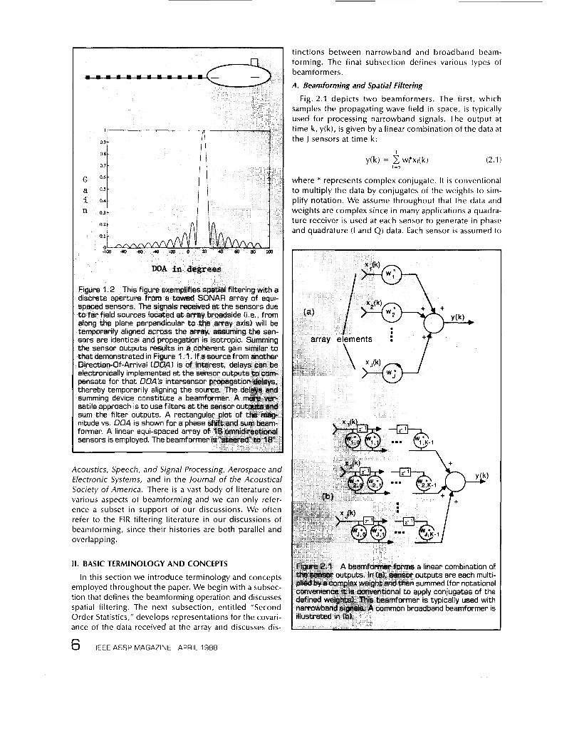
Several applications that employ spatial filtering of data are listed in Table 1 .1. Fig. 1 .I illustrates a microwave communications antenna that employs a continuous spatial aperture to accomplish spatial filtering with a single antenna. Fig. 1.2 depicts a low frequency-towed sonar array in which the spatial aperture is obtained through a discrete spatial sampling by an array of sensors. When the spatial sampling is discrete, the processor that performs the spatial filtering is termed a beamformer. Typically a

4 IEEE ASSP MAGAZINE APRIL 1988

Veen and Kevin M. Buckley

’igure 1 . I A continuous spatial aperture provides one nechanism for spatial filtering. Illustrated is a parabolic nicrowave antenna system. The antenna dish provides ;he spatial aperture over which energy is collected. This 3nergy is reflected to the antenna feed. The dish and feed iperate as a spatial integrator. The energy from a far field source located directly in front of the antenna arrives at ;he feed temporarily aligned [i.e., all source-to-feed path engths are equal1 and is coherently summed. In general, ?nergy from other sources will arrive at the feed via iariable length paths, and add incoherently. A polar plot if a typical antenna beampattern (i.e., power gain vs . , in ;his case, azimuth angle1 is shown for a selected fre- iuency and for the elevation angle at which the antenna is minted.

0740-746718810400-0004$01 .OOGI9881 EEE

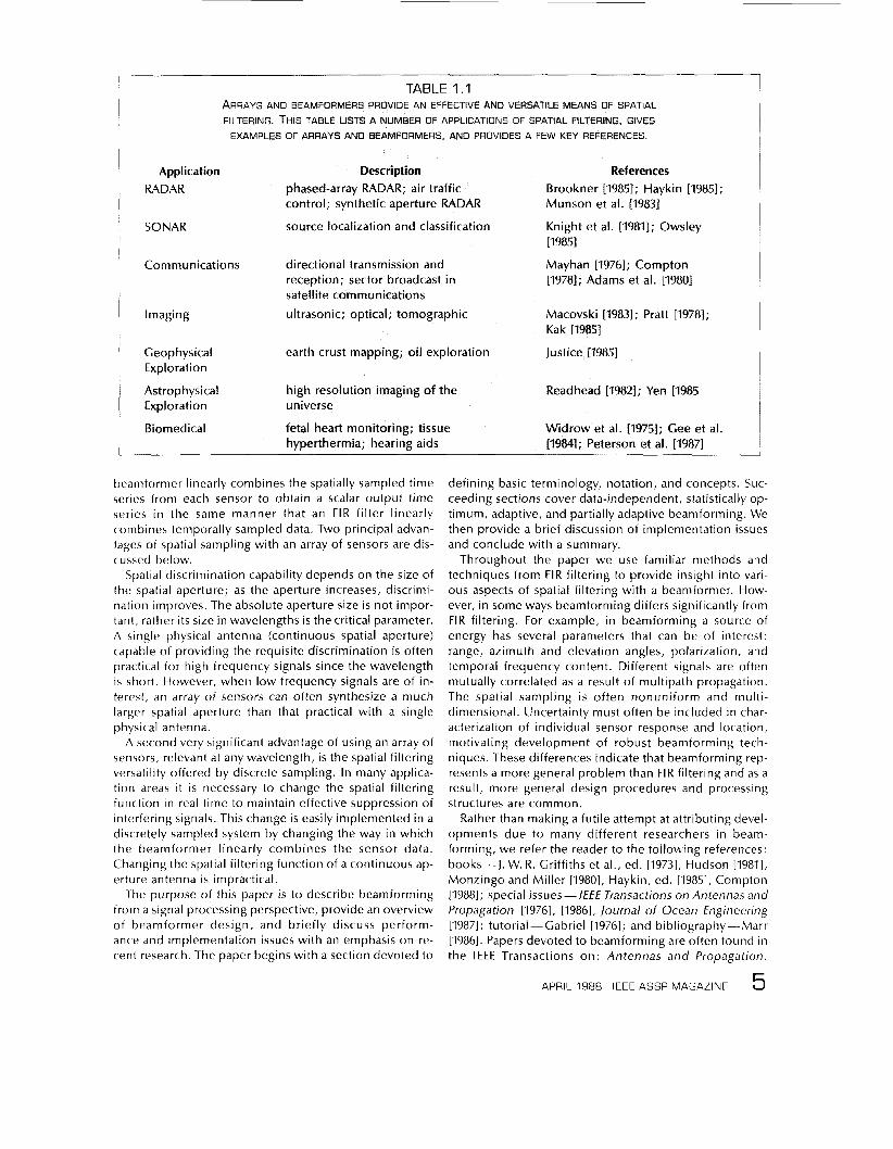
TABLE 1.1 ARRAYS AN0 BEAMFORMERS PROVIDE AN EFFECTIVE AND VERSATILE MEANS OF SPATIAL FILTERING. THIS TABLE LISTS A NUMBER OF APPLICATIONS OF SPATIAL FILTERING, GIVES

EXAMPLES OF ARRAYS AN0 BEAMFORMERS, AND PROVIDES A FEW KEY REFERENCES.

Application Description References

RADAR phased-array RADAR; air traffic Brookner [19851; Haykin 119851;

SONAR source localization and classification Knight et al. [19811; Owsley

Communications directional transmission and Mayhan 119761; Compton 119781; Adams et al. 119801

control; synthetic aperture RADAR Munson et al. (19831

[I9851

reception; sector broadcast in satellite communications

Imaging ultrasonic; optical; tomographic Macovski [19831; Pratt I19781;

Geophysical earth crust mapping; oil exploration Justice [I9851 Exploration

Astrophysical high resolution imaging of the Readhead [19821; Yen [I985 Exploration universe

Biomedical fetal heart monitoring; tissue

Kak [I9851

Widrow et al. 119751; Gee et al. [19841; Peterson et al. [I9871 hyperthermia; hearing aids

beamformer linearly combines the spatially sampled time series from each sensor to obtain a scalar output time series in the same manner that an FIR filter linearly combines temporally sampled data. Two principal advantages of spatial sampling with an array of sensors are discussed below.

Spatial discrimination capability depends on the size of the spatial aperture; as the aperture increases, discrimination improves. The absolute aperture size i s not important, rather its size in wavelengths is the critical parameter. A single physical antenna (continuous spatial aperture) capable of providing the requisite discrimination i s often practical for high frequency signals since the wavelength is short. However, when low frequency signals are of interest, an array of sensors can often synthesize a much larger spatial aperture than that practical with a single physical antenna.

A second very significant advantage of using an array of sensors, relevant at any wavelength, i s the spatial filtering versatility offered by discrete sampling. In many application areas it i s necessary to change the spatial filtering function in real time to maintain effective suppression of interfering signals. This change is easily implemented in a discretely sampled system by changing the way in which the beamformer linearly combines the sensor data. Changing the spatial filtering function of a continuous aperture antenna i s impractical.

The purpose of this paper is to describe beamforming from a signal processing perspective, provide an overview of beamformer design, and briefly discuss performance and implementation issues with an emphasis on recent research. The paper begins with a section devoted to

defining basic terminology, notation, and concepts. Suc- ceeding sections cover data-independent, statistically optimum, adaptive, and partially adaptive beamforming. We then provide a brief discussion of implementation issues and conclude with a summary.

Throughout the paper we use familiar methods and techniques from FIR filtering to provide insight into various aspects of spatial filtering with a beamformer. How- ever, in some ways beamforming differs significantly from FIR filtering. For example, in beamforming a source of energy has several parameters that can be of interest: range, azimuth and elevation angles, polarization, and temporal frequency content. Different signals are often mutually correlated as a result of multipath propagation. The spatial sampling i s often nonuniform and multidimensional. Uncertainty must often be included in char- acterization of individual sensor response and location, motivating development of robust beamforming techniques. These differences indicate that beamforming represents a more general problem than FIR filtering and as a result, more general design procedures and processing structures are common.

Rather than making a futile attempt at attributing developments due to many different researchers in beamforming, we refer the reader to the following references: books-J. W. R. Griffiths et al., ed. [19731, Hudson [19811, Monzingo and Miller [19801, Haykin, ed. [19851, Compton [19881; special issues - / € € E Transactions on Antennas and Propagation [19761, [19861, journal of Ocean Engineering [19871; tutorial - Gabriel [1976]; and bibliography- Marr [19861. Papers devoted to beamforming are often found in the IEEE Transactions on: Antennas and Propagation,

5 APRIL 1988 IEEE ASSP MAGAZINE

Acoustics, Speech, and Signal Processing, Aerospace and Electronic Systems, and in the lournal of the Acoustical Society of America. There is a vast body of literature on various aspects of beamforming and we can only reference a subset in support of our discussions. We often refer to the FIR filtering literature in our discussions of beamforming, since their histories are both parallel and overlapping .

I I . BASIC TERMINOLOGY AND CONCEPTS

In this section we introduce terminology and concepts employed throughout the paper. We begin with a subsection that defines the beamforming operation and discusses spatial filtering. The next subsection, entitled “Second Order Statistics,” develops representations for the covariance of the data received at the array and discusses dis-


tinctions between narrowband and broadband beamforming. The final subsection defines various types of beamformers.

A. Beam forming and Spatial Filtering

Fig. 2.1 depicts two beamformers. The first, which samples the propagating wave field in space, is typically used for processing narrowband signals. The output at time k, y(k), is given by a linear combination of the data at the J sensors at time k:

I y(k) = C w?xi(k) (2.1)

L=l

where * represents complex conjugate. It i s conventional to multiply the data by conjugates of the weights to simplify notation. We assume throughout that the data and weights are complex since in many applications a quadrature receiver i s used at each sensor to generate in phase and quadrature (I and Q) data. Each sensor i s assumed to

have any necessary receiver electronics and an N D con- verter if beamforming is performed digitally.

The second beamformer in Fig. 2.1 samples the propagating wave field in both space and time and is often used when signals of significant frequency extent (broadband) are of interest. The output in this case can be expressed as

(2.2)

where K - 1 is the number of delays in each of the J sensor channels. If the signal at each sensor is viewed as an input, then a beamformer represents a multi-input single output system.

It is convenient to develop notation which permits us to treat both beamformers in Fig. 2.1 simultaneously. Note that (2.1) and (2.2) can be written as

y(k) = wHx(k) . (2.3)

by appropriately defining a weight vector w and data vector x(k). We use lower and upper case boldface to denote vector and matrix quantities respectively, and let super- script H represent Hermitian (complex conjugate) trans- pose. Vectors are assumed to be column vectors. Assume that w and x(k) are N dimensional; this implies that N = KJ when referring to (2.2) and N = J when referring to (2.1). Except for Section V on adaptive algorithms, we will drop the time index and assume that i ts presence is understood throughout the remainder of the paper. Thus (2.3) i s written as y = wHx. Many of the techniques described in this paper are applicable to continuous time as well as discrete time beamforming.

The frequency response of an FIR filter with tap weights w;, 0 5 p 5 J and a tap delay of T seconds is given by

1 K-1

y(k) = c c WtpXl(k - P) I=1 p=o

I

p = l ,.(@) = W p + e - ~ ~ T ( ~ - l ) (2.4a)

Alternatively

r(w) = wHd(w) (2.4b)

where w H = [w? w;. . . WT] and d ( w ) = [ I eJwTe12wT . . . e ~ i l - l ) w T H 1 . r(o) represents the response of the filter to a complex sinusoid of frequency w and d(w) i s a vector describing the phase of the complex sinusoid at each tap in the FIR filter relative to the tap associated with wl.

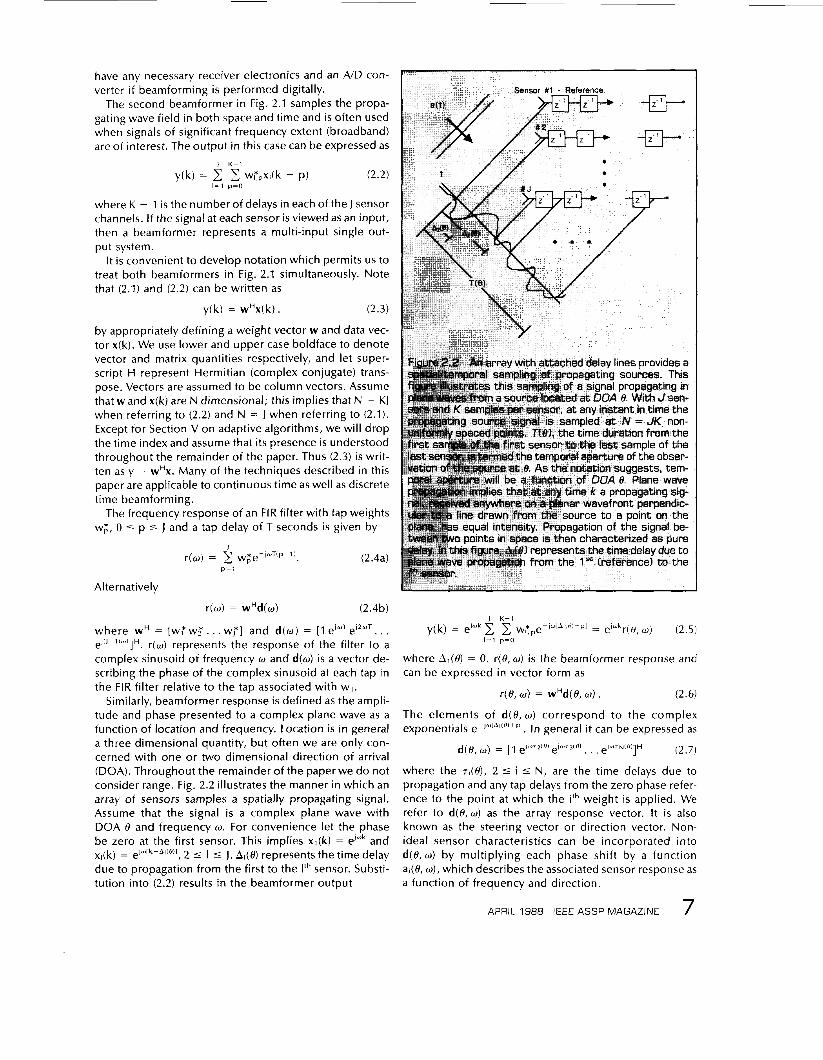
Similarly, beamformer response is defined as the amplitude and phase presented to a complex plane wave as a function of location and frequency. Location i s in general a three dimensional quantity, but often we are only concerned with one or two dimensional direction of arrival (DOA). Throughout the remainder of the paper we do not consider range. Fig. 2.2 illustrates the manner in which an array of sensors samples a spatially propagating signal. Assume that the signal i s a complex plane wave with DOA 8 and frequency w . For convenience let the phase be zero at the first sensor. This implies xl(k) = elwk and xdk) = eJw[k-AI'o)l, 2 5 I 5 J. Al(8) represents the time delay due to propagation from the first to the Ith sensor. Substi- tution into (2.2) results in the beamformer output

I Sensor #I - Reference

I Y-- l

y(k) = 2 '2' Wtpe- lWIA l (o )+P l - - eIwkr(8,w) (2.5) I=1 p=o

where A , ( @ = 0. r(0, w ) i s the beamformer response and can be expressed in vector form as

r(8, w ) = wHd(8, 0). (2.6)

The elements of d(8,w) correspond to the complex exponentials e-lw[Al(o)+P' . In general i t can be expressed as

d(8, w ) = [I eJWT2(o) e lWT3(8 ) . . . elwTN(@I]H (2.7)

where the 7,(8), 2 5 i 5 N, are the time delays due to propagation and any tap delays from the zero phase reference to the point at which the ith weight is applied. We refer to d(0,w) as the array response vector. It is also known as the steering vector or direction vector. Non- ideal sensor characteristics can be incorporated into d(8,w) by multiplying each phase shift by a function ado, w ) , which describes the associated sensor response as a function of frequency and direction.

APRIL 1988 IEEE ASSP MAGAZINE 7

The beampattern is defined as the magnitude squared of r(0,w). Note that each weight in w affects both the temporal and spatial response of the beamformer. His- torically, use of FIR filters has been viewed as providing frequency dependent weights in each channel. This interpretation is accurate but somewhat incomplete since the coefficients in each filter also influence the spatial filtering characteristics of the beamformer. As a multi-input single output system, the spatial and temporal filtering that occurs i s a result of mutual interaction between spatial and temporal sampling.

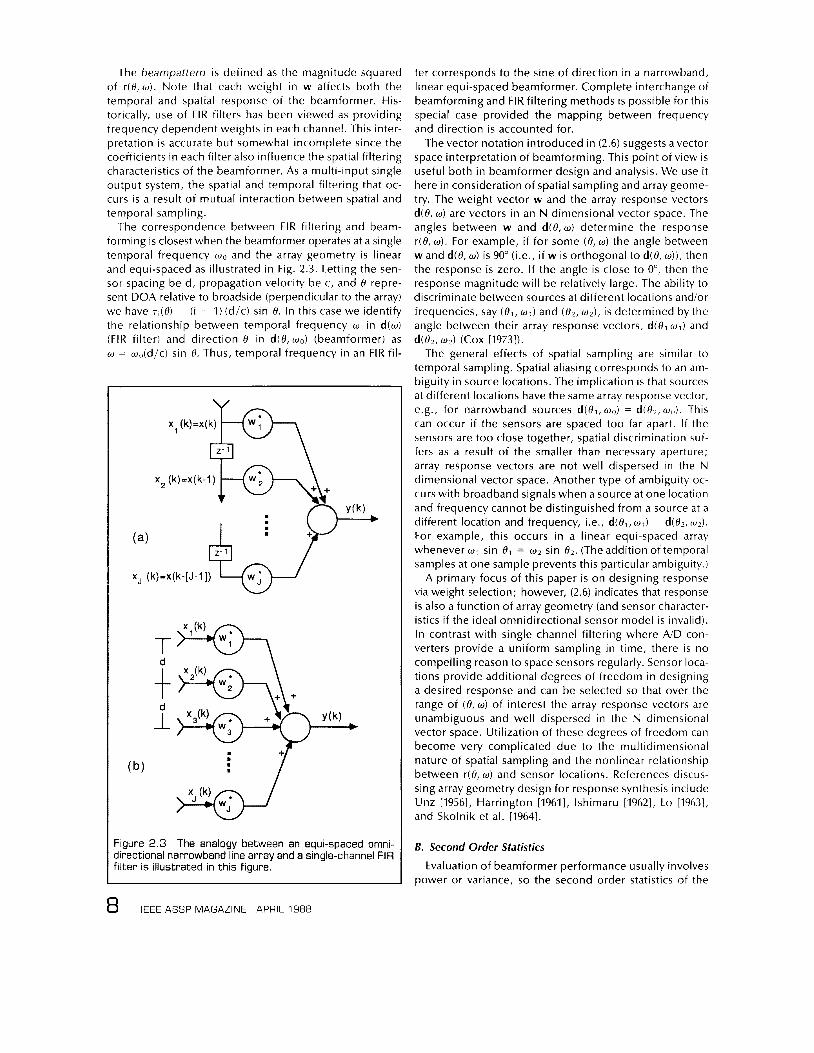
The correspondence between FIR filtering and beamforming i s closest when the beamformer operates at a single temporal frequency w,) and the array geometry i s linear and equi-spaced as illustrated in Fig. 2.3. Letting the sensor spacing be d, propagation velocity be c, and 0 represent DOA relative to broadside (perpendicular to the array) we have T , ( @ ) = (i - 1) (d/c) sin 0. In this case we identify the relationship between temporal frequency w in d(w) (FIR filter) and direction 0 in d(O,wO) (beamformer) as w = wo(d/c) sin 0. Thus, temporal frequency in an FIR fil-

m s

m m I Figure 2.3 The analogy between an equi-spaced omnidirectional narrowband line array and a single-channel FIR Filter is illustrated in this figure.

ter corresponds to the sine of direction in a narrowband, linear equi-spaced beamformer. Complete interchange of beamforming and FIR filtering methods i s possible for this special case provided the mapping between frequency and direction is accounted for.

The vector notation introduced in (2.6) suggests a vector space interpretation of beamforming. This point of view is useful both in beamformer design and analysis. We use it here in consideration of spatial sampling and array geometry. The weight vector w and the array response vectors d(0, w ) are vectors in an N dimensional vector space. The angles between w and d(0, w ) determine the response r(0, w). For example, if for some (0, w ) the angle between wand d(0, w ) is 90" (i.e., if w is orthogonal to d(0, w ) ) , then the response is zero. If the angle is close to o", then the response magnitude will be relatively large. The ability to discriminate between sources at different locations and/or frequencies, say (01, wl) and ( 0 2 , w 2 ) , i s determined by the angle between their array response vectors, d(0, w , ) and

The general effects of spatial sampling are similar to temporal sampling. Spatial aliasing corresponds to an ambiguity in source locations. The implication is that sources at different locations have the same array response vector, e.g., for narrowband sources d(Ol ,w0) = d(02,wo) . This can occur if the sensors are spaced too far apart. If the sensors are too close together, spatial discrimination suf- fers as a result of the smaller than necessary aperture; array response vectors are not well dispersed in the N dimensional vector space. Another type of ambiguity occurs with broadband signals when a source at one location and frequency cannot be distinguished from a source at a different location and frequency, i.e., d(&, w,) = d(02, w J . For example, this occurs in a linear equi-spaced array whenever w1 sin O1 = w 2 sin 0 2 . (The addition of temporal samples at one sample prevents this particular ambiguity.)

A primary focus of this paper is on designing response via weight selection; however, (2.6) indicates that response i s also a function of array geometry (and sensor characteristics if the ideal omnidirectional sensor model is invalid). In contrast with single channel filtering where AID con- verters provide a uniform sampling in time, there i s no compelling reason to space sensors regularly. Sensor locations provide additional degrees of freedom in designing a desired response and can be selected so that over the range of ( 0 , ~ ) of interest the array response vectors are unambiguous and well dispersed in the N dimensional vector space. Utilization of these degrees of freedom can become very complicated due to the multidimensional nature of spatial sampling and the nonlinear relationship between r(0, w ) and sensor locations. References discus- sing array geometry design for response synthesis include Unz [19561, Harrington [19611, lshimaru [19621, Lo [19631, and Skolnik et al. [19641.

d(02, ~ 2 ) (COX [19731).

B. Second Order Statistics

Evaluation of beamformer performance usually involves power or variance, so the second order statistics of the

data play an important role. We assume the data received at the sensors is zero mean throughout the paper. The variance or expected power of the beamformer output is given by E{/yI2} = wHE{xxH)w. If the data is wide sense stationary, then R, = E{xxH}, the data covariance matrix, is independent of time. Although we often encounter nonstationary data, the wide sense stationary assumption i s used in developing statistically optimal beamformers and in evaluating steady state performance.

Suppose x represents samples from a uniformly sampled time series having a power spectral density S(w) and no energy outside of the spectral band [ w a , o b ] . R, can be expressed in terms of the power spectral density of the data using the Fourier transform relationship as

with d(w) as defined for (2.4b). Now assume the array data x is due to a source located at direction 0. In like manner to the time series case we can obtain the covariance matrix of the array data as

S(w)d(O, o)dH(t), wi d o . (2.9)

A source i s said to be narrowband of frequency w g i f R, can be represented as the rank one outer product

(2.10)

R x = - \ 1 W b

277 " U a

R, = g?d(O, wo)dH(tl, woi

where (rs i s the source variance or power. The conditions under which a source can be considered

narrowband depend on both the source bandwidth and the time over which the source is observed. To illustrate this, consider observing an amplitude modulated sinusoid or the output of a narrowband filter driven by white noise on an oscilloscope. If the signal bandwidth i s small relative to the center frequency (i.e., i f it has a small fractional bandwidth), and the time intevals over which the signal i s observed are short relative to the inverse of the signal bandwidth, then each observed waveform has the shape of a sinusoid. Note that as the observation time interval is increased, the bandwidth must decrease for the signal to remain sinusoidal in appearance. It turns out, based on statistical arguments, that the observation time bandwidth product (TBWP) is the fundamental parameter that determines whether a source can be viewed as narrowband (Buckley [19871, Compton [19881).

An array provides an effective temporal aperture over which a source is observed. Fig. 2.2 illustrates this temporal aperture T(0) for a source arriving from direction 8. Clearly the TBWP is dependent on the source DOA. An array is considered narrowband if the observation TBWP is much less than one for all possible source directions.

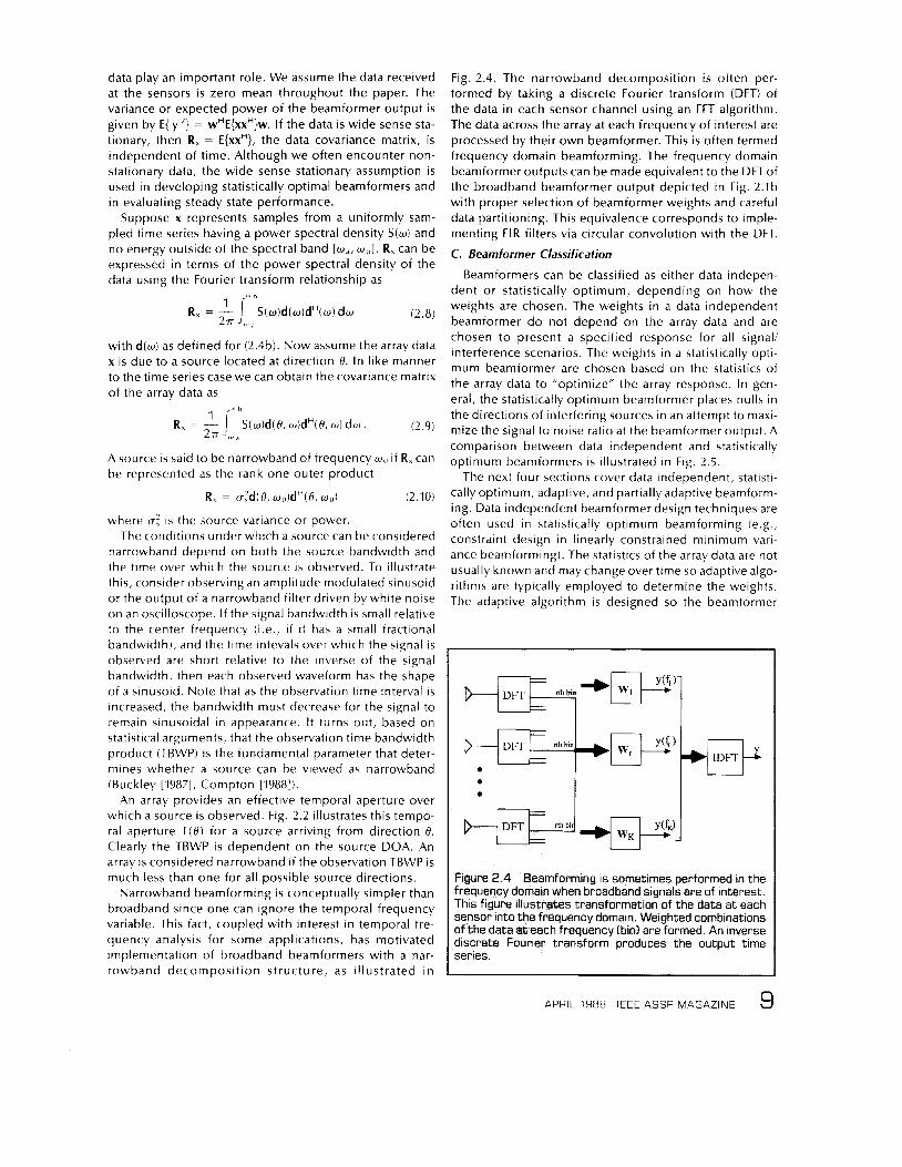
Narrowband beamforming is conceptually simpler than broadband since one can ignore the temporal frequency variable. This fact, coupled with interest in temporal frequency analysis for some applications, has motivated implementation of broadband beamformers with a narrowband decomposit ion structure, as illustrated in

Fig. 2.4. The narrowband decomposition is often performed by taking a discrete Fourier transform (DFT) of the data in each sensor channel using an FFT algorithm. The data across the array at each frequency of interest are processed by their own beamformer. This is often termed frequency domain beamforming. The frequency domain beamformer outputs can be made equivalent to the DFT of the broadband beamformer output depicted in Fig. 2.lb with proper selection of beamformer weights and careful data partitioning. This equivalence corresponds to implementing FIR filters via circular convolution with the DFT.

C. Beamformer Classification

Beamformers can be classified as either data independent or statistically optimum, depending on how the weights are chosen. The weights in a data independent beamformer do not depend on the array data and are chosen to present a specified response for all signal/ interference scenarios. The weights in a statistically optimum beamformer are chosen based on the statistics of the array data to "optimize" the array response. In general, the statistically optimum beamformer places nulls in the directions of interfering sources in an attempt to maximize the signal to noise ratio at the beamformer output. A comparison between data independent and Statistically optimum beamformers is illustrated in Fig. 2.5.

The next four sections cover data independent, statistically optimum, adaptive, and partially adaptive beamforming. Data independent beamformer design techniques are often used in statistically optimum beamforming (e.g., constraint design in linearly constrained minimum variance beamforming). The statistics of the array data are not usually known and may change over time so adaptive algorithms are typically employed to determine the weights. The adaptive algorithm is designed so the beamformer

0 I I U

series.

APRIL 1988 IEEE ASSP MAGAZINE 9

-80 -60 40 -20 0 20 40

Amvai Anelc~deereef

weight index

1

0 8 -

07 ~

1 0 6 - 3 0 5 -

% 04- 3

03 - 0 2 -

0 1 -

0- ~ 2 4 rli 8 IO

wngtl1 Indcx

ii 14

-100 -80 -60 -40 -7.0 0 20 40 60 80 1w

-60 -

-70 . -80 -lw -80 -60 40 -20 0 20 40 60 80 Io0

response be unity for an arrival angle of 18". Energy IS assumed to arrive a t the array from several interference

1 0 IEEE ASSP MAGAZINE APRIL 1988

response converges to a statistically optimum solution. Partially adaptive beamformers reduce the adaptive algorithm computational load at the expense of a loss (designed to be small) in statistical optimality.

Ill. DATA INDEPENDENT BEAMFORMING

The weights in a data independent beamformer are designed so the beamformer response approximates a desired response independent of the array data or data statistics. This design objective-approximating a desired response- is the same as that for classical FIR filter design (see, for example, Parks and Burrus [19871). We shall exploit the analogies between beamforming and FIR filtering where possible in developing an understanding of the design problem and in presenting design procedures. We also discuss design problems specific to beamforming.

The first part of this section discusses forming beams in a classical sense, i.e., approximating a desired response of unity at a point of direction and zero elsewhere. Methods for designing beamformers having more general forms of desired response are presented in the second part.

A. Classical Beamforming

Consider the problem of separating a single complex frequency component from other frequency components using the J tap FIR filter illustrated in Fig. 2.3. If frequency

is of interest, then the desired frequency response i s unity at w n and zero elsewhere. A common solution to this problem is to choose w as the vector d(w,). This choice can be shown to be optimal in terms of minimizing the squared error between the actual response and desired response. The actual response is characterized by a main lobe (or beam) and many sidelobes. Since w = d(w,), each element of w has unit magnitude. Tapering or windowing the amplitudes of the elements of w permits trading of main lobe or beam width against sidelobe levels to form the response into a desired shape. Let T be a J by J diagonal matrix with the real-valued taper weights as diagonal elements. The tapered FIR filter weight vector i s given by Td(w). A detailed comparison of a large number of tapering functions is given in Harris [1978].

In spatial filtering one is often interested in receiving a signal arriving from a known location point B o . Assuming the signal is narrowband (frequency wJ, a common choice for the beamformer weight vector i s the array reponse vector d(O,, U") . The resulting array and beamformer is termed a phased array since the output of each sensor is phase shifted prior to summation. Fig. 1.2 depicts the magnitude of the actual response when w = d(O,, w o ) . As in the FIR filter discussed above, beam width and sidelobe levels are the important characteristics of the response. Amplitude tapering can be used to control the shape of the response, i.e., to form the beam. Figs. 2.5a and b illustrate the effect of amplitude tapering on the response.

The equivalence of the narrowband linear equi-spaced array and FIR filter (see Fig. 2.3) implies that the same techniques for choosing taper functions are applicable to

Y / .. . . . . . . . . ~ , ~ ~ : : I I . .**.*.

. . . . . . . . . . . . . . . . . . . . . . . . . . . . .

. .

X

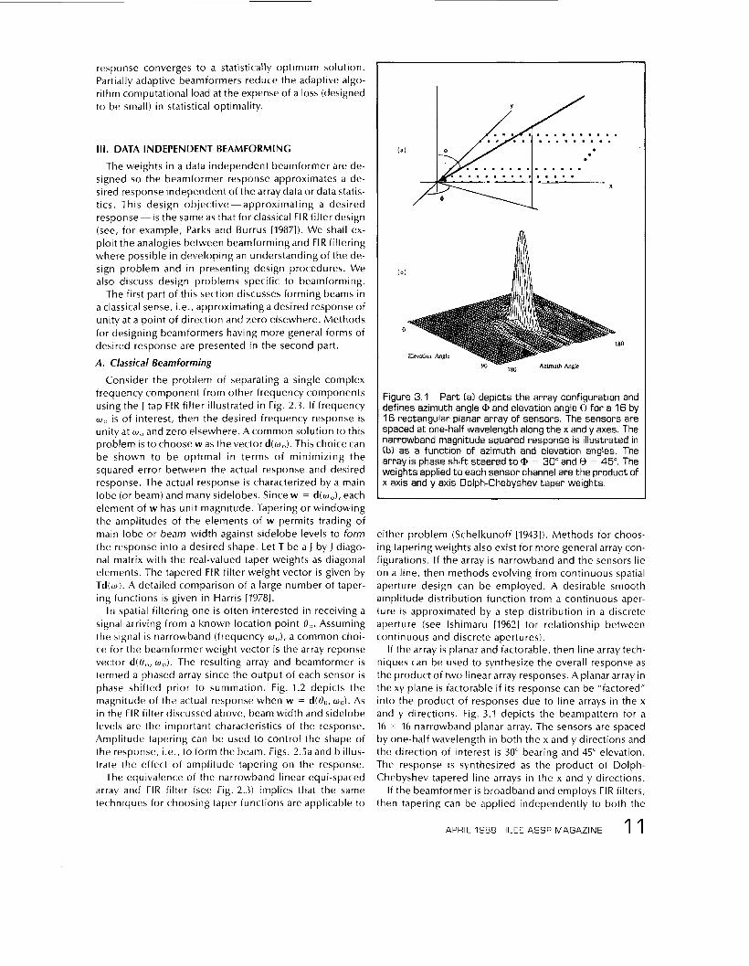
Figure 3.1 Part (a) depicts the array configuration and defines azimuth angle Q, and elevation angle 0 for a 16 by 16 rectangular planar array of sensors. The sensors are spaced at one-half wavelength along the x and y axes. The narrowband magnitude squared response is illustrated in Ibl as a function of azimuth and elevation angles. The array is phase shift steered to Q, = 30" and 0 = 45". The weights applied to each sensor channel are the product of x axis and y axis Dolph-Chebyshev taper weights.

either problem (Schelkunoff [19431). Methods for choosing tapering weights also exist for more general array con- figurations. If the array is narrowband and the sensors lie on a line, then methods evolving from continuous spatial aperture design can be employed. A desirable smooth amplitude distribution function from a continuous aperture is approximated by a step distribution in a discrete aperture (see lshimaru [I9621 for relationship between continuous and discrete apertures).

If the array i s planar and factorable, then line array techniques can be used to synthesize the overall response as the product of two linear array responses. A planar array in the xy plane i s factorable if its response can be "factored" into the product of responses due to line arrays in the x and y directions. Fig. 3.1 depicts the beampattern for a 16 x 16 narrowband planar array. The sensors are spaced by one-half wavelength in both the x and y directions and the direction of interest is 30" bearing and 45" elevation. The response is synthesized as the product of Dolph- Chebyshev tapered line arrays in the x and y directions.

If the beamformer is broadband and employs FIR filters, then tapering can be applied independently to both the

1 1 APRIL 1988 IEEE ASSP MAGAZINE

the desired source.

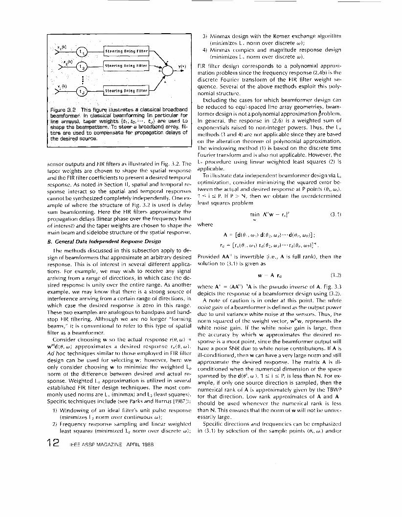
sensor outputs and FIR filters as illustrated in Fig. 3.2. The taper weights are chosen to shape the spatial response and the FIR filter coefficients to present a desired temporal response. As noted in Section I I , spatial and temporal response interact so the spatial and temporal responses cannot be synthesized completely independently. One example of where the structure of Fig. 3.2 is used is delay sum beamforming. Here the FIR filters approximate the propagation delays (linear phase over the frequency band of interest) and the taper weights are chosen to shape the main beam and sidelobe structure of the spatial response.

B. General Data Independent Response Design

The methods discussed in this subsection apply to design of beamformers that approximate an arbitrary desired response. This is of interest in several different applications. For example, we may wish to receive any signal arriving from a range of directions, in which case the desired response is unity over the entire range. As another example, we may know that there is a strong source of interference arriving from a certain range of directions, in which case the desired response is zero in this range. These two examples are analogous to bandpass and band- stop FIR filtering. Although we are no longer ”forming beams,” it is conventional to refer to this type of spatial filter as a beamformer.

Consider choosing w so the actual response r(O,w) = wHd(O, w ) approximates a desired response rd(O, w ) . Ad hoc techniques similar to those employed in FIR filter design can be used for selecting w; however, here we only consider choosing w to minimize the weighted L, norm of the difference between desired and actual response. Weighted L, approximation is utilized in several established FIR filter design techniques. The most com- monly used norms are L, (minmax) and L2 (least squares). Specific techniques include (see Parks and Burrus [19871):

1) Windowing of an ideal filter’s unit pulse response (minimizes L2 norm over continuous w ) ;

2) Frequency response sampling and linear weighted least squares (minimized L2 norm over discrete w ) ;


3) Minmax design with the Remez exchange algorithm

4) Minmax complex and magnitude response design

FIR filter design corresponds to a polynomial approximation problem since the frequency response (2.4b) is the discrete Fourier transform of the FIR filter weight sequence. Several of the above methods exploit this polynomial structure.

Excluding the cases for which beamformer design can be reduced to equi-spaced line array geometries, beamformer design is not a polynomial approximation problem. In general, the response in (2.6) is a weighted sum of exponentials raised to non-integer powers. Thus, the L, methods (3 and 4) are not applicable since they are based on the alteration theorem of polynomial approximation. The windowing method (1) is based on the discrete time Fourier transform and i s also not applicable. However, the L2 procedure using linear weighted least squares (2) i s applicable.

To illustrate data independent beamformer design via Lz optimization, consider minimizing the squared error between the actual and desired response at P points ( O , , w , ) , 1 5 i 5 P. I f P > N, then we obtain the overdetermined least squares problem

(minimizes L, norm over discrete w ) ;

(minimizes L, norm over discrete w ) .

i

min IAHw - rdlL (3.1) w

where

A = [d(Oq, w i ) d(O,, Wd*..d(Op, W P ) ] ;

rd = [Td(O,, w , ) rd(O2, W2)’..Td(OP, w d l H .

Provided AAH i s invertible (i.e., A i s full rank), then the solution to (3.1) i s given as

W = A+rd (3.2)

where A+ = (AAH)-’A i s the pseudo inverse of A. Fig. 3.3 depicts the response of a beamformer design using (3.2).

A note of caution is in order at this point. The white noisegain of a beamformer is defined as the output power due to unit variance white noise at the sensors. Thus, the norm squared of the weight vector, wHw, represents the white noise gain. If the white noise gain is large, then the accuracy by which w approximates the desired response is a moot point, since the beamformer output will have a poor SNR due to white noise contributions. If A i s ill-conditioned, then w can have a very large norm and still approximate the desired response. The matrix A i s ill- conditioned when the numerical dimension of the space spanned by the d(O’, w ’ ) , 1 5 i 5 P, is less than N. For example, if only one source direction is sampled, then the numerical rank of A i s approximately given by the TBWP for that direction. Low rank approximates of A and A’ should be used whenever the numerical rank i s less than N. This ensures that the norm of w will not be unnec- essarily large.

Specific directions and frequencies can be emphasized in (3.1) by selection of the sample points ( O , , w , ) and/or

sensors space

unequally weighting of the error at each ( f ? , , w , ) . Parks and Burrus [I9871 discuss this in the context of FIR filtering. Kumar and Murthy [I9771 consider unequal weighting of the error to obtain minimax response design for beamformer weights in a linear narrowband array. In general, guidelines for selection of the error weighting and ( O , , U , )

are not available.

There are several alternatives to L, optimization for general data independent response design, including methods discussed in Butler and Unz [I9671 and Sanzgiri and Butler [19711.

IV. STATISTICALLY OPTIMUM BEAMFORMING

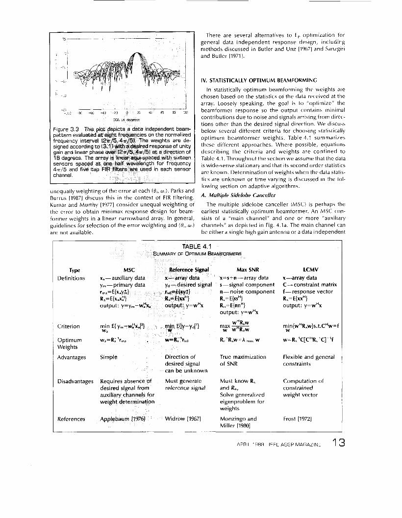
In statistically optimum beamforming the weights are chosen based on the statistics of the data received at the array. Loosely speaking, the goal i s to ”optimize” the beamformer response so the output contains minimal contributions due to noise and signals arriving from directions other than the desired signal direction. We discuss below several different criteria for choosing statistically optimum beamformer weights. Table 4.1 summarizes these different approaches. Where possible, equations describing the criteria and weights are confined to Table 4.1. Throughout the section we assume that the data i s wide-sense stationary and that its second order statistics are known. Determination of weights when the data statistics are unknown or time varying i s discussed in the following section on adaptive algorithms.

A. Multiple Sidelobe Canceller

The multiple sidelobe canceller (MSC) is perhaps the earliest statistically optimum beamformer. An MSC consists of a ”main channel” and one or more “auxiliary channels” as depicted in Fig. 4.la. The main channel can be either a single high gain antenna or a data independent

Type Definitions

Optimum wa=R;’rma Weights

Advantages Simple Direction of desired signal can be unknown

Disadvantages Req Must generate reference signal

Max SNR x=s+n-array data s-signal component n-noise component R,= E{&} R,=E{nnH} output: y=wHx

RZ1R,w=h w

True maximization of SNR

Must know R, and R,, Solve generalized eigenproblem for weights

Monzingo and Miller [I9801

LCMV x -a r ray data C- constraint matrix f- response vector R,=E{xx~} output: y=wHx

rnin{w”R,w}s.t.CHw=f W

w = R, IC[ C R;’C]-’f

Flexible and general constraints

Computation of constrained weight vector

Frost 11972)

APRIL 1988 IEEE ASSP MAGAZINE 1 3

main channel response

V main channel

auxiliary branch response 1

auxiliary channels

a) b)

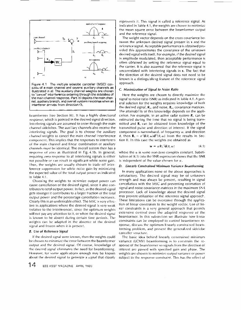
Figure 4.1 The multiple sidelobe canceller [MSCI consists of a main channel and several auxiliary channels as illustrated in a1 The auxiliary channel weights are chosen to “cancel” interference entering through the sidelobes of the main channel response. Part b l depicts the main channel, auxiliary branch, and overall system response when an interferer arrives from direction 8,.

beamformer (see Section I l l ) . It has a highly directional response, which i s pointed in the desired signal direction. Interfering signals are assumed to enter through the main channel sidelobes. The auxiliary channels also receive the interfering signals. The goal is to choose the auxiliary channel weights to cancel the main channel interference component. This implies that the responses to interferers of the main channel and linear combination of auxiliary channels must be identical. The overall system then has a response of zero as illustrated in Fig. 4.lb. In general, requiring zero response to all interfering signals i s either not possible or can result in significant white noise gain. Thus, the weights are usually chosen to trade off interference suppression for white noise gain by minimizing the expected value of the total output power as indicated in Table 4.1.

Choosing the weights to minimize output power can cause cancellation of the desired signal, since it also contributes to total output power. In fact, as the desired signal gets stronger it contributes to a larger fraction of the total output power and the percentage cancellation increases. Clearly this is an undesirable effect. The MSC is very effective in applications where the desired signal i s very weak (relative to the interference), since the optimum weights will not pay any attention to it, or when the desired signal i s known to be absent during certain time periods. The weights can be adapted in the absence of the desired signal and frozen when it is present.

B. Use of Reference Signal

If the desired signal were known, then the weights could be chosen to minimize the error between the beamformer output and the desired signal. Of course, knowledge of the desired signal eliminates the need for beamforming. However, for some applications enough may be known about the desired signal to generate a signal that closely


represents it. This signal is called a reference signal. As indicated in Table 4.1, the weights are chosen to minimize the mean square error between the beamformer output and the reference signal.

The weight vector depends on the cross covariance between the unknown desired signal present in x and the reference signal. Acceptable performance is obtained provided this approximates the covariance of the unknown desired signal with itself. For example, i f the desired signal i s amplitude modulated, then acceptable performance i s often obtained by setting the reference signal equal to the carrier. It is also assumed that the reference signal is uncorrrelated with interfering signals in x. The fact that the direction of the desired signal does not need to be known is a distinguishing feature of the reference signal approach.

C. Maximization of Signal to Noise Ratio

Here the weights are chosen to directly maximize the signal to noise ratio (SNR) as indicated in Table 4.1. A general solution for the weights requires knowledge of both the desired signal, R,, and noise, R,, covariance matrices. The attainability of this knowledge depends on the application. For example, in an active radar system R , can be estimated during the time that no signal is being transmitted and R, can be obtained from knowledge of the transmitted pulse and direction of interest. If the signal component i s narrowband, of frequency w , and direction 8, then R, = c2d(0 ,w)dH(0 ,w) from the results in Sec- tion II. In this case the weights are obtained as

w = aRL’d(8, 0) (4.1)

where the (Y is some non-zero complex constant. Substi- tution of (4.1) into the SNR expression shows that the SNR is independent of the value chosen for a .

D. Linearly Constrained Minimum Variance Beamforming

In many applications none of the above approaches i s satisfactory. The desired signal may be of unknown strength and may always be present, resulting in signal cancellation with the MSC and preventing estimation of signal and noise covariance matrices in the maximum SNR processor. Lack of knowledge about the desired signal may prevent utilization of the reference signal approach. These limitations can be overcome through the application of linear constraints to the weight vector. Use of linear constraints is a very general approach that permits extensive control over the adapted response of the beamformer. In this subsection we illustrate how linear constraints can be employed to control beamformer response, discuss the optimum linearly constrained beamforming problem, and present the generalized sidelobe canceller structure.

The basic idea behind linearly constrained minimum variance (LCMV) beamforming i s to constrain the response of the beamformer so signals from the direction of interest are passed with specified gain and phase. The weights are chosen to minimize output variance or power subject to the response constraint. This has the effect of

preserving the desired signal while minimizing contributions to the output due to interfering signals and noise arriving from directions other than the direction of interest. The analogous FIR filter has the weights chosen to minimize the filter output power subject to the constraint that the filter response to signals of frequency w o be unity.

In Section II we saw that the beamformer response to a source at angle 8 and temporal frequency w i s given by wHd(8, U ) . Thus, by linearly constraining the weights to satisfy wHd(8, w ) = g, where g i s a complex constant, we ensure that any signal from angle 0 and frequency U is passed to the output with response g. Minimization of contributions to the output from interference (signals not arriving from 6, with frequency w ) i s accomplished by choosing the weights to minimize the expected value of output power or variance E{jyj2} = wHR,w. The LCMV problem for choosing the weights i s thus written

"2 w"R,w subject to dH(H,w)w = g*. (4.2)

The method of Lagrange multipliers can be used to solve (4.2) resulting in

R;'d( 8, U )

d"(8, w)R['d(O, w ) w = g* (4.3)

Note that in practice the presence of uncorrelated noise will ensure that R, i s invertible. If g = 1, then (4.3) is often termed the minimum variance distortionless response (MVDR) beamformer. It can be shown that (4.3) is equivalent to the maximum SNR solution given in (4.1) by substi- tuting cr2d(8,w)dH(6,,w) + R, for R, in (4.3) and applying the matrix inversion lemma.

The single linear constraint in (4.2) is easily generalized to multiple linear constraints for added control over the beampattern. For example, if there i s a fixed interference source at a known direction 6, then it may be desirable to force zero gain in that direction in addition to maintaining the response g to the desired signal. This is expressed as

(4.4)

If there are L < N linear constraints on w, we write them in the form CHw = f where the N by L matrix C and L dimensional vector f are termed the constraint matrix and response vector. The constraints are assumed to be linearly independent so C has rank L. The LCMV problem and solution with this more general constraint equation are given in Table 4.1.

Constraint Design. Several different philosophies can be employed for choosing the constraint matrix and response vector. We discuss point (Kelly and Levin [19641), deriv&ive (Owsley [1973], Er and Cantoni [1983]), and eigenvector (Buckley [1987]) constraints below. In many applications, a combination of the different types of constraints is most effective. Each linear constraint uses one degree of freedom in the weight vector so with L constraints there are only N - L degrees of freedom available for m i n irnizing variance.

Point constraints fix the beamformer response at points of spatial direction and temporal frequency. Equation (4.4) represents an example of two point constraints on w. The number of points at which response can be constrained i s limited to N . If N constraints are used then there are no degrees of freedom left for power minimization and a data independent beamformer i s obtained.

Derivative constraints are employed to influence response over a region of direction and/or frequency by forcing the derivatives of the beamformer response at some point of direction and frequency to be zero. They are usually employed in conjunction with point constraints. An example where derivative constraints are useful is when the desired signal direction i s only known approximately. If the signal arrives near the direction at which a point constraint i s employed, then application of a derivative constraint at that point prevents the beamformer from synthesizing a response of zero to the desired signal.

Eigenvector constraints are based on a least squares approximation to the desired response and are typically used to control beamformer response over regions of direction and/or frequency. Constraining the beamformer response in a least squares sense ensures that the mean square error between desired and actual beamformer response over a region is minimized for a given number of constraints. In this sense eigenvector constraints are efficient. Consider designing a set of constraints which will control the beamformer response to a source from direction 8, over the frequency band [w , ,ub ] . The dimension of the span of d(O,,w) over this band i s approximately given by the source TBWP discussed in Section I I . Eigenvector constraints are derived from (3.1) by choosing P significantly greater than the TBWP. The w , then oversample [ua, w b l and A is ill-conditioned. A rank L approximation of A i s obtained from its singular value decomposition

AL = VZ LUH (4.5)

where XL i s an L by 1. diagonal matrix containing the largest singular values of A, and the L columns of V and U are respectively the left and right singular vectors of A corresponding to these singular values. Replacing A in (3.1) by its rank L approximate (4.5) and bringing UC, to the right side (the pseudo inverse of U i s U"), yields

Equation (4.6) has the same form as the constraint equation CHw = f . The columns of V correspond to the eigen- vectors of AAH; hence the name eigenvector Constraints. (Note that AAH represents an approximation of R, in (2.9) if S ( w ) = 1.)

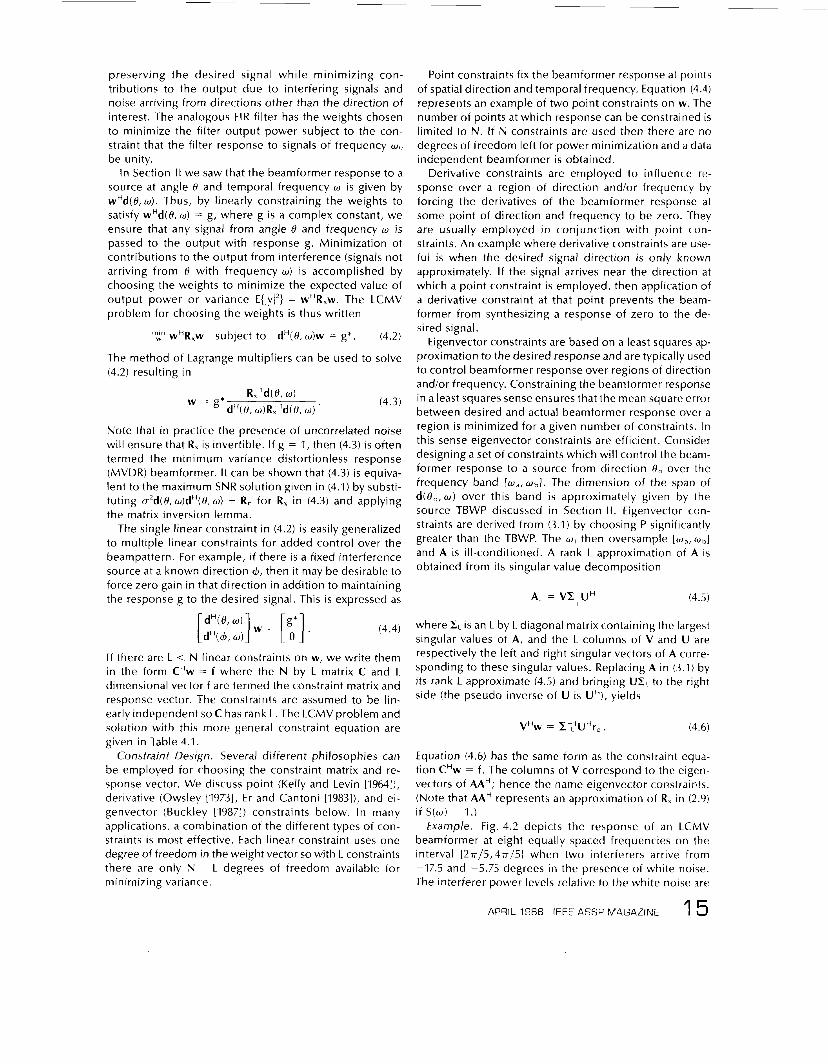
Example. Fig. 4.2 depicts the response of an LCMV beamformer at eight equally spaced frequencies on the interval [ 2 ~ / 5 , 4 ~ / 5 1 when two interferers arrive from -17.5 and -5.75 degrees in the presence of white noise. The interferer power levels relative to the white noise are


icts the LCMV beamformer

51 when two inter-

151 and have powers of 40

30 and 40 dB, respectively, and the interferers have a flat spectrum on [ 2 ~ / 5 , 4 ~ / 5 ] . The array has sixteen linear equi-spaced sensors with five taps per sensor. The tap spacing i s normalized to one second and the sensors are spaced at one-half wavelength corresponding to frequency 4 ~ / 5 . The response is constrained to pass signals arriving from 18 degrees in the band [ 2 ~ / 5 , 4 ~ / 5 ] , with unit gain and linear phase using ten eigenvector constraints designed from (4.6). The effectiveness of the constraints is evident, since all the frequency curves pass through zero dB at 18 degrees. The response has nulls in the directions of the interferers with the deeper null corresponding to the stronger interferer. The response as a function of frequency for the interferer directions is plot- ted in Fig. 6.2. The array gain is 50 dB for this example.

Generalized Sidelobe Canceller. The generalized sidelobe canceller (GSC) represents an alternative formulation of the LCMV problem, which provides insight, is useful for analysis, and can simplify LCMV beamformer implementation. It also illustrates the relationship between the MSC and LCMV beamforming. Essentially, the CSC is a mecha- nism for changing a constrained minimization problem into unconstrained form. Perhaps the first reference to this concept is in Hanson and Lawson [19691, where a procedure for transforming constrained least squares problems to unconstrained least squares problems i s given. Griffiths and Jim [I9821 applied the same concept to LCMV beamforming and coined the term GSC. Similar techniques were discussed in Applebaum and Chapman [1976].

Suppose we decompose the weight vector w into two orthogonal components w, and -v (w = wo - v) that lie in the range and null space of C, respectively. The range and null space of a matrix span the entire space so this

I 6 IEEE ASSP MAGAZINE APRIL 1988

decomposition can be used to represent any w. Since CHv = 0, we must have

WO = C(CHC)-’f (4.7)

if w i s to satisfy the constraints. (4.7) i s the minimum L, norm solution to the underdetermined equivalent of (3.1). The vector v i s a linear combination of the columns of an N by N-L matrix C,(v = C,w,) provided the columns of C, form a basis for the null space of C. C, can be obtained from C using any of several orthogonalization procedures such as Gram-Schmidt, QR decomposition, or singular value decomposition. The weight vector w = w, - Cnw,, is depicted in block diagram form in Fig. 4.3. The choice for w, and C, implies that w satisfies the constraints independent of wn and reduces the LCMV problem to the unconstrained problem

Gnn[wo - CnwnIHRx[wo - Cnwn]. (4.8)

The solution i s

w, = (C!R,C,) -’C:R,w,. (4.9)

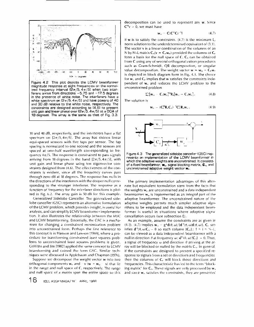
Figure 4.3 The generalized sidelabe canceller (GSCI rep- beamformer in

ned. I t consists matrix, C,, and

The primary implementation advantages of this alter- nate but equivalent formulation stem from the facts that the weights w, are unconstrained and a data independent beamformer w, is implemented as an integral part of the adaptive beamformer. The unconstrained nature of the adaptive weights permits much simpler adaptive algorithms to be employed and the data independent beamformer i s useful in situations where adaptive signal cancellation occurs (see subsection E).

As an example, assume the constraints are as given in (4.2). (4.7) implies w, = g*d(H, w)/[dH(8, w)d(O, w ) ] . C, satisfies dH(8,w)C,, = 0 so each column [ C , , ] , ; 1 5 i 5 N-L, can be viewed as a data independent beamformer with a null in direction 0 at frequency w : dH(8, w ) [C,,], = 0. Thus, a signal of frequency w and direction 8 arriving at the array will be blocked or nulled by the matrix c,, . In general, if the constraints are designed to present a specified response to signals from a set of directions and frequencies, then the columns of C, will block those directions and frequencies. This characteristic has led to the term “blocking matrix” for C,. These signals are only processed by wc, and since w, satisfies the constraints, they are presented

with the desired response independent of w,,. Signals from directions and frequencies over which the response i s not constrained will pass through the upper branch in Fig. 4.3 with some response determined by w,. The lower branch chooses wn to estimate the signals at the output of w0 as a linear combination of the data at the output of the blocking matrix. This is similar to the operation of the MSC, in which weights are applied to the output of auxiliary sensors in order to estimate the primary channel output (see Fig. 4.1).

E. Signal Cancellation in Statistically Optimum Beam forming.

Optimum beamforming requires some knowledge of the desired signal characteristics, either its statistics (for maximum SNR or reference signal methods), its direction (for the MSC), or its response vector d(0, w ) (for the LCMV beamformer). If the required knowledge is inaccurate, the optimum beamformer will attenuate the desired signal as i f it were interterence. Cancellation of the desired signal i s often significant, especially if the SNR of the desired signal is large (Cox [1973]). Several approaches have been suggested to reduce this degradation (e.g., Jablon [19861, Cox et al. 119871).

A second cause of signal cancellation i s correlation between the desired signal and one or more interference signals. This can result either from multipath propagation of a desired signal or from smart (correlated) jamming. When interference and desired signals are uncorrelated the beamformer attenuates interferers to minimize output power. However, with a correlated interferer the beamformer minimizes output power by processing the interfering signal in such a way as to cancel the desired signal. If the interferer is partially correlated with the desired signal, then the beamformer will cancel the portion of the desired signal that i s correlated with the interferer. Meth- ods for reducing signal cancellation due to correlated interference have been suggested (e.g., Widrow et al. [19821, Shan and Kailath [19851, Yang and Kaveh [19871).

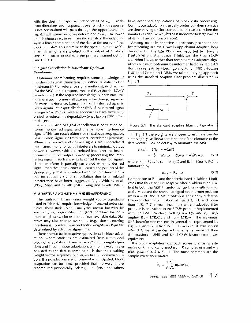
, ? - I : I 1 Figure 5.1 The standard adaptive filter configuration.

V. ADAPTIVE ALGORITHMS FOR BEAMFORMING

The optimum beamformer weight vector equations listed in Table 4.1 require knowledge of second order statistics. These statistics are usually not known, but with the assumption of ergodicity, they (and therefore the optimum weights) can be estimated from available data. Sta- tistics may also change over time (e.g., due to moving interferers). To solve these problems, weights are typically determined by adaptive algorithms.

There are two basic adaptive approaches: 1) block adaptation, where statistics are estimated from a temporal block of array data and used in an optimum weight equation; and 2) continuous adaptation, where the weights are adjusted as the data i s sampled such that the resulting weight vector sequence converges to the optimum solution. If a nonstationary environment is anticipated, block adaptation can be used, provided that the weights are recomputed periodically. Adams, et al. [I9801 and others

have described applications of block data processing. Continuous adaptation is usually preferred when statistics are time-varying or (for computational reasons) when the number of adaptive weights M i s moderate to large (values of M > 50 are not uncommon).

Among notable adaptive algorithms proposed for beamforming are the Howells-Applebaum adaptive loop developed in the late 1950's and reported by Howells [1966,1976] and Applebaum [1966], and the Frost LCMV algorithm [19721. Rather than recapitulating adaptive algorithms for each optimum beamformer listed in Table 4.1 (for this see texts by Monzingo and Miller [1980], Hudson [I9811 and Compton [1988]), we take a unifying approach using the standard adaptive filter problem illustrated in Fig. 5.1.

I I

1 K-1

K k = U R, = - c u(k)u"(k)


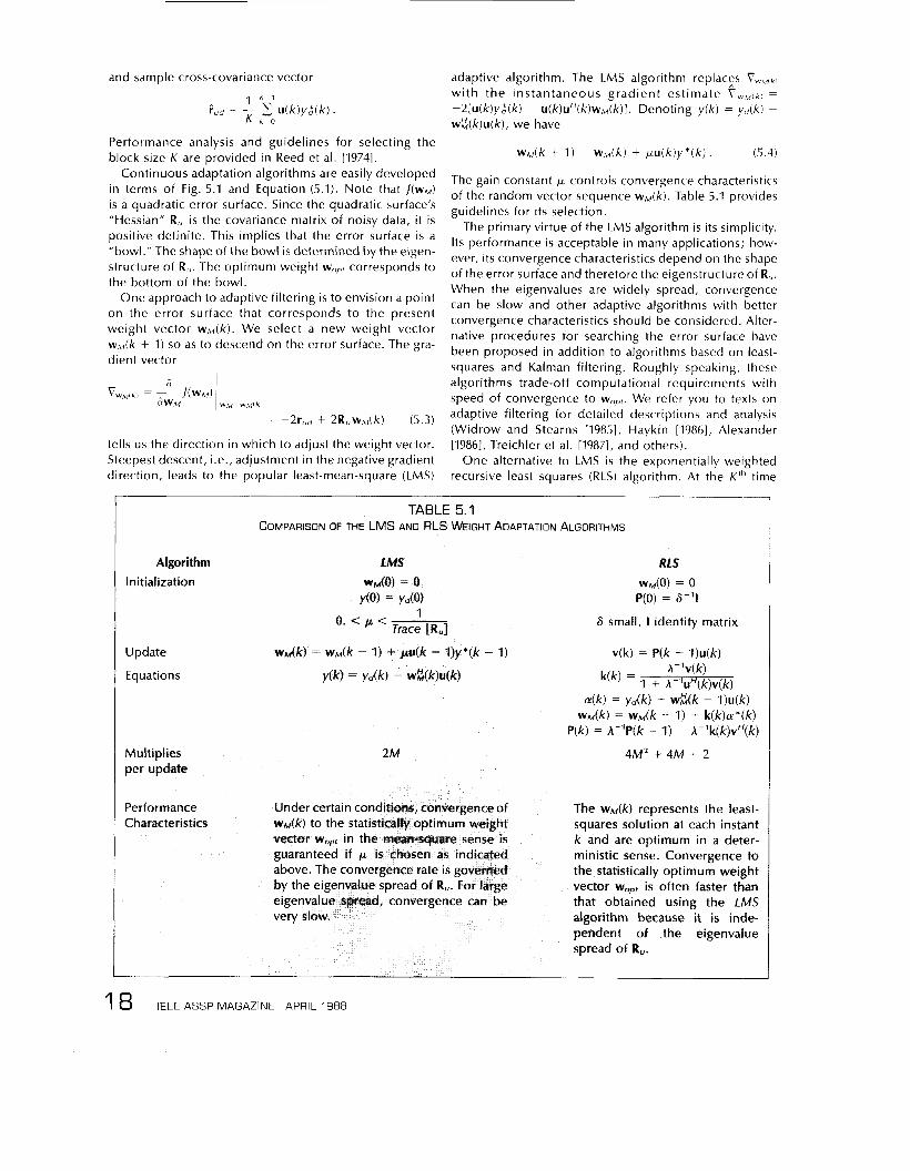
and sample cross-covariance vector

a V w M t k ) = - / ( W M )

dWM WM wM(kl

adaptive algorithm. The L M S algorithm replac:s Ywu(kl

wi th the instantaneous gradient estimate V w , , ( k , =

-2 [u (k )yd (k ) - u ( k ) u ” ( k ) w M ( k ) l . Denoting y (k ) = yd(k) - w % k ) u ( k ) , we have

WM(k + 1) = WM(k) + p u ( k ) y * ( k ) . (5.4)

The gain constant p controls convergence characteristics of the random vector sequence w d k ) . Table 5.1 provides guidelines for its selection.

The primary virtue of the LMS algorithm is its simplicity. Its performance is acceptable in many applications; however, its convergence characteristics depend on the shape of the error surface and therefore the eigenstructure of R,. When the eigenvalues are widely spread, convergence can be slow and other adaptive algorithms with better convergence characteristics should be considered. Alter- native procedures for searching the error surface have been proposed in addition to algorithms based on least- squares and Kalman filtering. Roughly speaking, these algorithms trade-off computational requirements with speed of convergence to wept. We refer you to texts on adaptive filtering for detailed descriptions and analysis (Widrow and Stearns 119851, Haykin [19861, Alexander [1986], Treichler et al. [1987], and others).

One alternative to LMS is the exponentially weighted recursive least squares (RLS) algorithm. At the Kth time

Algorithm Initialization

Update

Equations

Multiplies per update

Performance Characteristics

TABLE 5.1 COMPAAJSON OF THE LMS AND RLS WEIGHT ADAPTATtON ALGORITHMS

2M

RLS

WM(0) = 0 P(0) = rll

6 small, I identity matrix

v(k) = P(k - I)u(k)

k(k) = 1 f h-’uH(k)v(k) X-’v(k)

a (k) = y&) - wZ(k - l)u(k) W M ( ~ ) = w M ( ~ - I) + k(k)a*(k)

P(k) = h-’P(k - 1) - A-‘k(k)vH(k)

4M* f 4M + 2

The w d k ) represents the least- squares solution at each instant k and are optimum in a deter- ministic sense. Convergence to the statistically optimum weight vector wept is often faster than that obtained using the LMS algorithm because it is independent of the eigenvalue spread of R,.

I 8 ~ E E E ASSP MAGAZINE APRIL 1988

step, wM(K) i s chosen to minimize a weighted sum of past squared errors

K

min AK-kIyd(k) - w%K)u(k)/'. (5.5) W M ( K ) k 0

A i s a positive constant less than one which determines how quickly previous data are deemphasized. The RLS algorithm is obtained from (5.5) by expanding the magnitude squared and applying the matrix inversion lemma. Table 5.1 summarizes both the L M S and RLS algorithms.

VI. INTERFERENCE CANCELLATION AND PARTIALLY ADAPTIVE BEAMFORMING

The computational requirements of each update in adaptive algorithms are proportional to either the weight vector dimension M or dimension squared (M'). If M i s large, this requirement is quite severe and for practical real time implementation it i s often necessary to reduce M.

The expression degrees o f freedom refers to the number of unconstrained or "free" weights in an implementation. For example, an LCMV beamformer with L constraints on N weights has N-L degrees of freedom; the GSC implementation separates these as the unconstrained weight vector wn. There are M degrees of freedom in the structure of Fig. 5.1. A fully adaptive beamformer uses all available degrees of freedom and apartiallyadaptive beamformer uses a reduced set of degrees of freedom. Re- ducing degrees of f reedom lowers computational requirements and often improves adaptive response time.' However, there is a performance penalty associated with reducing degrees of freedom. A partially adaptive beamformer cannot converge to the same optimum solution as the fully adaptive beamformer. The goal of partially adaptive beamformer design is to reduce degrees of freedom without significant degradation in performance.

The discussion in this section is general, applying to different types of beamformers although we borrow much of the notation from the GSC. We assume the beamformer i s described by the adaptive structure of Fig. 5.1 where the desired signal yd i s obtained as yd = w,"x and the data vector U as U = THx. Thus, the beamformer output is y = wHx where w = wo - TwM. In order to distinguish between fully and partially adaptive implementations we decompose T into a product of two matrices C,TM. The definition of C, depends on the particular beamformer and TM represents the mapping which reduces degrees of freedom. The MSC and GSC are obtained as special cases of this representation. In the M S C wo i s an N vector that selects the primary sensor, C, is an N by N-I matrix that selects the N-I possible auxiliary sensors from the complete set of N sensors, and TM i s an N-I by M matrix that selects the M auxiliary sensors actually utilized. In terms of

'Adaptive algorithm convergence characteristics have not been discussed in this paper. Generally, more data are required to derive an accurate estimate of a larger optimum weight vector with block adaptive processing or RLS [Reed et al., 19741. With LMS, convergence is governed by the covariance matrix eigenvalue spread, which tends to be larger for larger dimensional problems.

the GSC, w, and C, are defined as in Section IV and TM i s an N-L by M matrix that reduces degrees of freedom

This section begins by considering the interference cancellation process in these general beamformer implementations. This develops the intuition required for understanding why and how the number of adaptive weights can be reduced. We conclude this section by surveying different partially adaptive beamformer design philosophies.

A. Interference Cancellation Vs Degrees of Freedom. The results in this subsection depend on T and are inde-

pendent of the individual terms C, and TM. We assume that the beamformer does not cancel the desired signal (see Section 1V.E.) and that the optimum weights affect only interferers and uncorrelated noise. This simplifies the analysis by permitting us to exclude consideration of the desired signal.

Suppose a narrowband interfering source of frequency w o arrives at the array from direction 0, . The response of the w, branch i s g, = w,Hd(O,, w o ) . Perfect cancellation of this source requires wHd(Ol,w,) = 0 so we must choose WM to satisfy

WETHd(O,, wC1) = gi . (6.1)

If we asume that THd(O,, w,) i s nonzero, (6.1) represents a system of one equation in M unknowns (elements of wM) for which a solution always exists. To simultaneously cancel a second interferer located at 0 2 , wM must satisfy

(M < N-L).

where g 2 = w,Hd(O,, w o ) . Assuming THd(B,, w o ) and THd(f12, U,) are linearly independent and nonzero, and provided M 2 2, then at least one whl exists that satisfies (6.2). Continuing this reasoning, we see that wM can be chosen to cancel M narrowband interferers (assuming the THd(O,, w,) are linearly independent and nonzero), independent of T. Total cancellation occurs i f wM i s chosen so the response of TwM perfectly matches the wo branch response to the interferers.

So far we have only considered narrowband point interferers. Uncorrelated noise will be present in any real system and contributes to the output power. In an optimum beamformer wM i s chosen to minimize the overall output power. Recall that the output power due to uncorrelated noise is proportional to the L2 norm squared of the overall weight vector w (white noise gain). The norm of w can become large when wM i s chosen to provide total interference cancellation, depending on the choice for T and the interferer locations. Thus, although in principle point sources of energy in direction and frequency can be totally canceled with one weight per interferer independent of T, the presence of uncorrelated noise results in the degree of cancellation being dependent on the mapping described by T.

Now consider interferers that are spatial point sources but emit broadband energy on the band w a 5 w 5 wh. The response of the w, branch to an interferer at 0 , is w,Hd(e,, w ) = gl(w). To achieve total cancellation wM must


be chosen to satisfy

WzTHd(OT,W) = g i (w) w a 5 w 5 w b . (6.3a)

Define the response of each column of T as

f,(w) = [T]?d(O,,w) 1 5 i 5 M (6.3b)

where [TI, denotes the ith column of T. (6.3a) requires gl (w) to be expressed as a linear combination of the f,(w), 1 5 i 5 M, on w , 5 w 5 wb. In general, this cannot be accomplished and we conclude that total cancellation of broadband interference cannot be obtained. The output power due to the broadband interferer can be expressed as the integral over frequency of the magnitude squared of the difference between the wo branch and adaptive branch responses weighted by the interferer power spectrum. The degree of cancellation can vary dramatically and i s critically dependent on the interferer direction, frequency content, and choice for T. Good cancellation can be obtained in some situations when M = 1, while in others even large values of M result in poor cancellation. These conclusions are also valid for narrowband sources that are broad in direction (spatially distributed radiation).

B. Partially Adaptive Beamformer Design.

The preceding discussion indicates that the degree of interference cancellation is critically dependent on the ability of the adaptive channel (TWM) to match the main beam response over the interferer frequency extent. This provides a means by which to evaluate partially adaptive beamformers. The majority of work reported on partially adaptive beamforming has been concerned with narrowband environments. We begin with a discussion of several narrowband approaches and briefly discuss their ex- tension to broadband situations. We then consider techniques that are directly applicable to broadband situations. Some techniques select Thl for a given C , while others select T directly.2

Several approaches to reducing degrees of freedom are based on processing a subset of the outputs of the matrix C , . This implies that TM i s a sparse matrix of zeros and ones. The outputs of C , in the MSC are simply auxiliary sensor outputs. Morgan [I9781 evaluated partially adaptive beamformer performance when TM selected various sub- sets of the auxiliary outputs. This i s termed an element space approach, since a subset of the sensor element outputs i s utilized. Several investigators, including Vural [19771, Adams, et al. [19801, and Gabriel [1986al have considered choosing the columns of T to form beams. This is traditionally termed a beam space approach. The columns of C,, are designed as data independent beamformers, each steered to a different direction, and TM can be used to select a subset of the beam outputs. The objective i s to direct a beam at each interfering source so that it can be subtracted from the output of thew, branch. One way to

'In principle one can generate auxiliary constraints in an LCMV beamformer to reduce the number of adaptive weights in a GSC implementation (Griffiths (19871). Here we assume all constraints are already specified in partially adaptive LCMV beamforming.

accomplish this i s by selecting enough beams to cover al l possible directions from which interferers might arrive. Another is to utilize source direction finding techniques to select which beams correspond to estimated interferer directions. The biggest advantage of the element space approach i s the simplicity of implementation. Improved performance obtained using beam space processing i s especially evident for interference due to either spatially distributed sources or sources with appreciable temporal bandwidth. However, this improvement i s obtained at the expense of implementing the required beams.

Chapman 119761 and Owsley [I9781 have considered choosing the columns of T to select subarrays, i.e., each column involves only a subset of the sensors in the array. The weightings applied to each subarray (elements of T) can be chosen in various ways, one of which i s to use the subarray to form a beam. Performance depends on the number of sensors in each subarray, which sensors are used in each subarray, and the weightings used to com- bine the sensor outputs in each subarray. Note that each column of T will have zeros in locations corresponding to sensors excluded from that subarray, so the overall T i s of sparse structure.

Owsley [I9851 suggests a narrowband method for the GSC in which the columns of TM are chosen as a basis for the space spanned by the fully adaptive weight vectors. The dimension of this space is given by the rank of the spatially correlated component of the interference covariance matrix. Van Veen [1988a] extended this approach to the broadband case. The dimension of the fully adaptive space can be large in this case since it i s given by the rank of the correlated components of the broadband interference covariance matrix.

The above approaches are capable of satisfactory performance with narrowband interference since cancellation requires about one degree of freedom per interferer to match the main beam response at each interferer direction. However, with broadband interference the main beam response must be matched over a range of frequency at each interferer direction. Although the narrowband approaches can be extended, it is difficult to do this and keep the number of adaptive weights M small. For example, several banks of beams could be designed to span the range of directions, with each bank operating at different frequency. The problem is that the number of beams required can become large as the frequency bandwidth increases. We seek aT that i s efficient, i.e., provides good cancellation with a minimum of columns.

Van Veen and Roberts [1987a] have considered an optimization based approach for choosing the columns of T in the context of LCMV beamforming. The matrix C, , i s designed to meet the constraints, reducing the problem to an unconstrained optimization over the elements of TU. TM i s chosen to minimize the average interference output power over a range of likely interference environments. Let a vector (Y parameterize the interference environment of interest. In general a can represent interferer locations, power levels, spectral distributions, numbers of in-


terferers, etc. Defining PI(@) as the interference output power, TM i s chosen according to

min 1, Pl(a) d a (6.4)

where [a,, (Yb] denotes the set of interference scenarios of interest. Since output power corresponds to the error between the w, branch and adaptive channel responses, in effect (6.4) selects TM to provide the best response match possible for interference environments in [aa , ab ] .

Equation (6.4) represents a design problem that is nonlinear in the design parameters (elements of TM). A suboptimal approach to solving (6.4), in which TM i s se- quentiallydesigned one column at a time, has been shown to be effective in achieving near fully adaptive interference cancellation using a small adaptive dimension. The problem i s still nonlinear; however an effective approximate solution is obtained by solving a linear least squares problem. An interpretation of this approximate solution i s given in Van Veen [1988b].

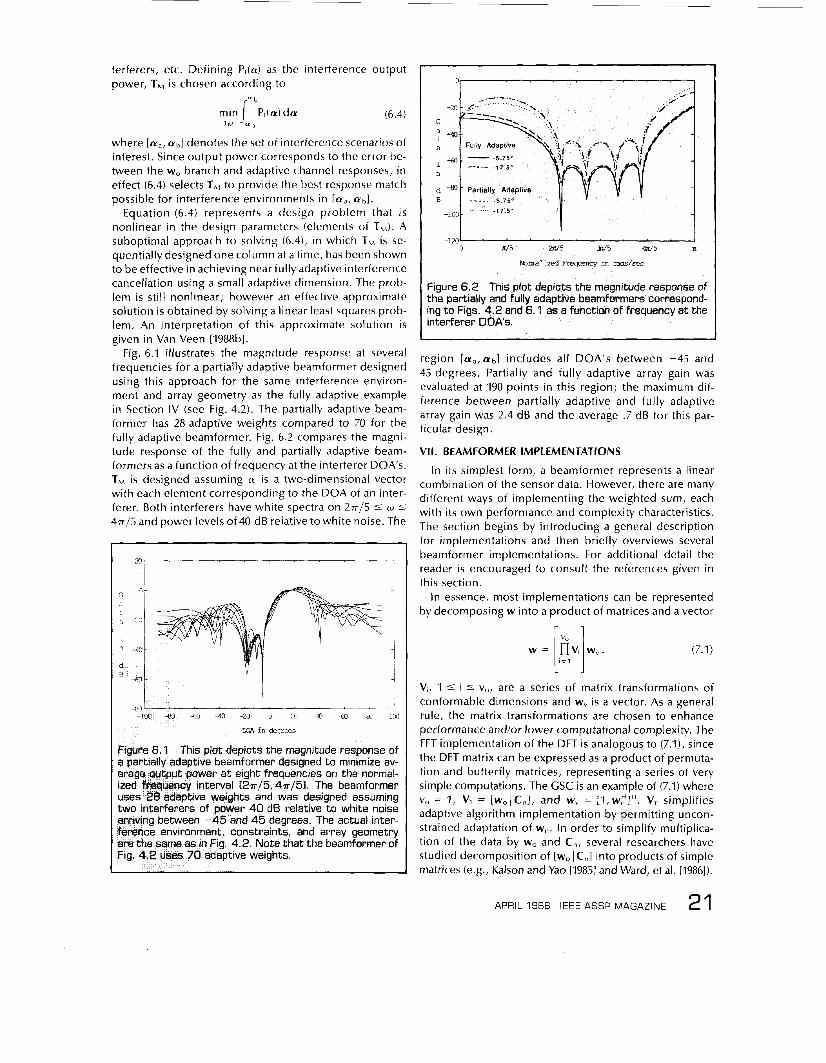
Fig. 6.1 illustrates the magnitude response at several frequencies for a partially adaptive beamformer designed using this approach for the same interference environment and array geometry as the fully adaptive example in Section IV (see Fig. 4.2). The partially adaptive beamformer has 28 adaptive weights compared to 70 for the fully adaptive beamformer. Fig. 6.2 compares the magnitude response of the fully and partially adaptive beamformers as a function of frequency at the interferer DOA's. TM i s designed assuming (Y is a two-dimensional vector with each element corresponding to the DOA of an interferer. Both interferers have white spectra on 2 ~ / 5 s o s 4 ~ / 5 and power levels of 40 dB relative to white noise. The

TM a

WA 1n degrees

o t depicts the magnitude response of beamformer designed to minimize av- r a t eight frequencies on the normal-

Val [2n/5,4s/51. The beamformer ights and was designed assuming

power 40 dB relative to white noise -45 and 45 degrees. The actual inter-

nt, constraints, and array geometry ig. 4.2. Note that the beamformer of

Figure 6.2 This plot gnitude response of the partially and fully formers correspond-

on of frequency a t the

I region [a,,abl includes all DOA's between -45 and 45 degrees. Partially and fully adaptive array gain was evaluated at 190 points in this region; the maximum difference between partially adaptive and fully adaptive array gain was 2.4 dB and the average .7 dB for this particular design.

VII. BEAMFORMER IMPLEMENTATIONS

In its simplest form, a beamformer represents a linear combination of the sensor data. However, there are many different ways of implementing the weighted sum, each with its own performance and complexity characteristics. The section begins by introducing a general description for implementations and then briefly overviews several beamformer implementations. For additional detail the reader i s encouraged to consult the references given in this section.

In essence, most implementations can be represented by decomposing w into a product of matrices and a vector

w = nv, w,. (7.1 1 [iy,

V,, 1 5 i 5 v,, are a series of matrix transformations of conformable dimensions and wv i s a vector. As a general rule, the matrix transformations are chosen to enhance performance and/or lower computational complexity. The FFT implementation of the DFT is analogous to (7.1), since the DFT matrix can be expressed as a product of permuta- tion and butterfly matrices, representing a series of very simple computations. The GSC is an example of (7.1) where v, = 1, V, = [w,/C,], and w, = [1,w,HIH. VI simplifies adaptive algorithm implementation by permitting unconstrained adaptation of wn. In order to simplify multiplica- tion of the data by w, and C,, several researchers have studied decomposition of [w, IC,] into products of simple matrices (e.g., Kalson and Yao [I9851 and Ward, et al. [19861).


As discussed in Section II, broadband beamforming can be performed in the frequency domain or time domain. The weights used to obtain the outputs at each frequency for the frequency domain beamformer depicted in Fig. 2.4 are easily represented in terms of (7.1) by employing the matrix representation of the DFT. Frequency domain optimum beamformers usually choose the weights at each frequency based solely on the data at the frequency. This partitioning of the data influences both performance and computational complexity. Discussion and evaluation of frequency domain beamforming is given in Owsley [1985], Vural [1977], and Gabriel [1986bl.

Systolic implementations of optimum beamformers have been studied by a number of investigators. They are usually designed to both compute and implement the adaptive weights. In general, systolic implementations can be described in terms of (7.1) where each V, has a structure amenable to parallel computation and local communication. McWhirter [I9831 (see also Haykin [I9861 ch. I O ) has developed a systolic array that computes the beamformer output without explicit computation of the adaptive weight vector. Additional references to systolic implementations include Schreiber and Kuekes [1985], Ward, et al. [19861, Owsley 119871, and Van Veen and Roberts [1987bl.

The study of beamformer implementations is an evolving research area. Future developments will result from advances in VLSl and parallel computing technologies.

VIII. S U M M A R Y

A beamformer forms a scalar output signal as a weighted combination of the data received at an array of sensors. The weights determine the spatial filtering characteristics of the beamformer and enable separation of signals having overlapping frequency content if they originate from different locations. The weights in a data independent beamformer are chosen to provide a fixed response independent of the received data. Statistically optimum beamformers select the weights to optimize the beamformer response based on the statistics of the data. The data statistics are often unknown and may change with time so adaptive algorithms are used to obtain weights that converge to the statistically optimum solution. Computational considerations dictate the use of partially adaptive beamformers with arrays cornposed of large numbers of sensors. Many different approaches have been proposed for implementing optimum beamformers. Future work will likely address signal cancellation problems, further reduc- tions in computational load for large arrays and improved structures for implementation. Beamforming truly represents a versatile approach to spatial filtering.

REFERENCES

Adams, R. N., Horowitz, L. L. and Senne, K. D. [1980], “Adaptive main-beam nulling for narrow-beam antenna arrays,” / € € E Trans. on AES, Vol. 16, pp. 509-516, Jul, 1980.

Alexander, S. T. [1986], Adaptive Signal Processing: Theory

and Applications, Springer-Verlag, New York, 1986. Applebaum, S. P. [1966], ”Adaptive arrays,” Syracuse Un.

Research Corp., Report SURC SPL TR 66-001, Aug. 1966 (reprinted in / € E € Trans. on AP, Vol. AP-24, pp. 585-598, Sept. 1976).

Applebaum, S. P. and Chapman, D. J . [1976], ”Adaptive arrays with main beam constraints,” /E€€ Trans. on AP, Vol. AP-24, pp. 650-662, Sept. 1976.

Brookner, E . [1985], ”Phased-array radar,” Scientific American, Vol. 252, pp. 94-102, Feb. 1985.

Buckley, K. M. [1987], “Spatialispectral filtering with I i n ear I y-co n s t ra i n ed m i n i m u rn va r i an ce beam f o r m e rs , “ / E € € Trans. on ASSP, Vol. ASSP-35, pp. 249-266, Mar. 1987.

Butler, J. K. and Unz, E. [1967], ”Beam efficiency and gain optimization of antenna arrays with nonuniform spac- ings,” Radio Sci., Vol. 2, pp. 711-720, 1967.

Chapman, D. J. [1976], ”Partial adaptivity for the large arrays,” / E € € Trans. on AP, Vol. 24, pp. 685-696, Sept. 1976.

Compton, Jr., R.T. [1978], “An adaptive array in a spread- spectrum communication system,” Proc. /€€€, Vol. 66, pp. 289-298, Mar. 1978.

Compton, Jr., R. T. [1988], Adaptive Antennas: Concepts and Performance, Prentice-Hall, Englewood Cliffs, New Jersey, 1988.

Cox, H. [1973], ”Resolving power and sensitivity to mismatch of optimum array processors,” lour. Acoust. Soc. Amer., Vol. 54, No. 3, pp. 771-785, 1973.

Cox, H., Zeskind, R. M. and Owen, M. M. [1987], “Robust adaptive beamforming,” / € E € Trans. on ASSP, Vol. ASSP-

Dolph, C. L. [1946], “A current distribution for broadside arrays which optimizes the relationship between beam width and side-lobe level,” Proc. o f IRE, Vol. 34, pp. 335-348, June 1946.

Er, M. H. and Cantoni, A. [1983], ”Derivative constraints for broad-band element space antenna array processors,” / € € E Trans. on ASSP, Vol. ASSP-31, pp. 1378-1393. Dec. 1983.

Frost Ill, 0. L. [1972], “An algorithm for linearly constrained adaptive array processing,” Proc. /€€€, Vol. 60,

Gabriel, W. F. [1986a], ”Using spectral est imation techniques in adaptive processing antenna systems,” / € E € Trans. on AP, Vol. 34, pp. 291-300, Mar. 1986.

Gabriel, W. F. [1986b], ”Adaptive digital processing investi- gation of DFT subbanding vs. transversal filter canceller,” NRL Report 8981, July, 1986.

Gabriel, W. F. [19761, ”Adaptive arrays-an introduction,” Proc. / € E € , Vol. 64, pp. 239-272, Aug. 1976.

Gee, W., Lee, S., Bong, N. K., Cain, C.A., Mittra, R. and Magin, R. L. [1984], “Focused array hyperthermia appli- cator: theory and experiment,” / € E € Trans. on BME, Vol. BME-31, pp. 38-45, Jan. 1984.

Criffiths, J. W. R., et al., ed. [19731, Signal Processing, Aca- demic Press, 1973.

Criffiths, L. J. and Jim, C. W. [19821, “An alternative ap-

35, pp. 1365-1375, Oct. 1987.

pp. 926-935, Aug. 1972.


proach to linearly constrained adaptive beamforming,” /€€E Trans. on AP, Vol. AP-30, pp. 27-34, Jan. 1982.

Griffiths, L. J. [1987], “A new approach to partially adaptive arrays,“ Proc. ICASSP-87, pp. 1999-2002, Apr. 1987.

Hanson, R.L. and Lawson, C.L. [19691, “Extensions and applications of the Householder algorithm for solving linear least squares problems,” Math. Comp., Vol. 23,

Harrington, R. F. [19611, “Sidelobe reduction by nonuniform element spacing,” IRE Trans. on AP, Vol. AP-9, pp. 187-192, Mar. 1961.

Harris, F. J . [1978], “On the use of windows for harmonic analysis with the discrete Fourier transform,” Proc. o f / E € € , Vol. 66, pp. 51-83, Jan. 1978.

Haykin, S., ed. [1985], Array Signal Processing, Prentice- Hall, Englewood Cliffs, New Jersey, 1985.

Haykin, S. [19861, Adaptive Filter Theory, Prentice-Hall, Englewood Cliffs, New Jersey, 1986.

Howells, P. W. [19661, “Intermediate frequency sidelobe canceller,” U.S. Patent 3202990, Aug. 1966.

Howells, P. W. [1976], “Explorations in fixed and adaptive resolut ion at GE and SURC,” /€€E Trans. on AP, Vol. AP-24, pp. 575-584, Sept. 1976.

Hudson, J . E. [1981], Adaptwe Array Principles, Peter Pere- grinus Ltd., London, 1981.

Ishimaru, A. [19621, ”Theory of unequally-spaced arrays,” IRE Trans. on AP, Vol. AP-10, pp. 691-702, Nov. 1962.

Jablon, N. K. [19681, “Steady state analysis of the generalized sidelobe canceller by adaptive noise cancelling techniques,” /€E€ Trans. on AP, Vol. AP-34, pp. 330-337, March 1986.

Justice, J . H. [1985], in Array Signal Processing, S . Haykin, ed., Prentice-Hall, Englewood Cliffs, New Jersey, 1985.

Kak, A.C. [1985], in Array Signal Processing, S . Haykin, ed., Prentice-Hall, Englewood Cliffs, New Jersey, 1985.

Kalson, S. and Yao, K. [1985], “A systolic array for linearly constrained least squares filtering,” Proc. ICASSP-85, pp. 977-980, Mar. 1985.

Kelly, Jr., E. L. and Levin, M. L. [1964], “Signal parameter estimation for seismometer arrays,” Mass. Inst. Tech., Lincoln Lab., Tech. Report 339, Jan. 1964.

Knight, W. C., Pridham, R. G. and Kay, S . M. [1981], ”Digital signal processing for sonar,” Proc. I € € € , Vol. 69, pp. 1451-1506, Nov. 1981.

Kumar, A. and Murthy, P. K. [1977], ”Synthesis of equally excited linear arrays,“ IRE Trans. on AP, Vol. AP-25, pp. 425-428, May 1977.

Lo, Y. T. [19631, “Sidelobe level in nonuniformly spaced antenna arrays,” /€€€ Trans. on Af‘, Vol. AP-11, pp. 511-512, July 1963.

Macovski, A. [19831, Medical Imaging, Prentice-Hall, Englewood Cliffs, New Jersey, 1983.

Marr, J . [19861, “A selected bibliography on adaptive antenna arrays,“ /E€€ Trans. on AES, Vol. AES-22, pp. 781-798, Nov. 1986.

Mayhan, J. T. [1976], ”Nulling limitations for a multiple- beam antenna,” / E € € Trans. on AP, Vol. 24, pp. 769-779, Nov. 1976.

pp. 917-926, 1969.

McWhirter, J . G. [1983], ”Recursive least-squares minimization using a systolic array,” Proc. SPlE 431, pp. 105- 112, 1983.

Monzingo, R. and Miller, T. [19801, lntroduction to Adap- tive Arrays, Wiley and Sons, New York, 1980.

Munson, Jr., D.C., O’Brian, J. D. and Jenkins, W. K. [19831, “A tomographic formulation of spot-light mode synthetic aperture radar,” Proc. /E€€, Vol. 71, pp. 917-925, Aug. 1983.

Morgan, D. R. [19781, ”Partially adaptive array techniques,” /E€€ Trans. on AP, Vol. 26, pp. 823-833, Nov. 1978.

Owsley, N. L. [19731, “A recent trend in adaptive spatial processing for sensor arrays: constrained adaptation,” in S igna l Processing, ed., J . W. R. Griffiths, et al., pp. 591-604, Academic Press, 1973.

Owsley, N. L. [19851, in Array Signal Processing, S. Haykin, ed., Prentice-Hall, Englewood Cliffs, New Jersey, 1985.

Owsley, N. L. [1987], ”Systolic array adaptive beamforming,” Naval Underwater Systems Center Report 7971, April, 1987.

Parks, T. W. and Burrus, C. S . [19871, Digital Filter Design, Wi ley-I n terscience, New York, 1987.

Peterson, P. M., Durlach, N. I., Rabinowitz, W.M. and Zurek, P. M. [1987], “Multimicrophone adaptive beamforming for interference reduction in hearing aids,” Jour. of Rehab. R&D, Vol. 24, Fall 1987.

Pratt, W. K. [19781, Digital lmage Processing, Wiley and Sons, New York, 1978.

Readhead, A. [1982], ”Radio astronomy by very-long- baseline interferometry,” Scientific American, Vol. 246, pp. 52-61, June 1982.

Reed, I . S., Mallett, J. D. and Brennen, L. E. [19741, “Rapid convergence rate in adaptive arrays,” I€€€ Trans. on AES,

Sanzgiri, S. M. and Butler, J. K. [1971], ”Constrained optimization of the performance indices of arbitrary array antennas,” I€€€ Trans. on AP, Vol. AP-19, pp. 725-730, July 1971.

Schelkunoff, S. A. [1943], “A mathematical theory of linear arrays,“ Bell Sys. Tech. Jour., Vol. 22, pp. 80-107, Jan. 1943.

Schreiber, R. and Kuekes, P. J. [19851, in VLSl a n d Modern Signal Processing, S. Y. Kung, H. J . Whitehouse and T. Kailath, eds., Prentice-Hall, Englewood Cliffs, New Jersey, 1985.

Shan, T. and Kailath, T. [1985], ”Adaptive beamforming for coherent signals and interference,” /E€€ Trans. on ASSP, Vol. ASSP-33, pp. 527-536, June 1985.

Skolnik, M. I . , Nemhauser, G. and Sherman, J . W. [19641, “Dynamic programming applied to unequally spaced arrays,“ I E E E Trans. on AP, Vol. AP-12, pp. 35-43. Jan. 196.1.

Treichler, J . R., Johnson, Jr., C. R. and Larimore, M.G. [19871, Theory and Design o f Adaptive Filters, Wiley- Interscience, New York, 1987.

Unz, H. [1956], “Linear arrays with arbitrarily distributed elements,“ U . of Cal., Berkeley, Elect. Reac. Lab, Rept. 168, Nov. 1956.

Van Veen, B. D. and Roberts, R.A. [1987al, ”Partially adap-

Vol. AES-10, pp. 853-863, NOV. 1974.

tive beamformer design via output power minimization," / € € E Trans. on ASSP, Vol. ASSP-35, pp. 1534-1532, Nov. 1987.

Van Veen, B. D. and Roberts, R. A. [1987b], "Systolic arrays for partially adaptive beamforming," 27-st Asilomar Con- ference o n Signals, Systems, a n d Computers,

Van Veen, B. D. [1988a], "Eigenstructure based partially adaptive array design," / E € € Trans. on AP, Vol. AP-36, pp. 357-362, Mar. 1988.

Van Veen, B. D. [1988b], "improved power minimization based partially adaptive beamforming," ICASSP-88, Apr. 1988.

Vural, A. M. [1977], "A comparative performance study of adaptive array processors," Proc. ICASSP-77, pp. 695- 700, Apr. 1977.

Ward, C. R., Hargrave, P. J. and McWhirter, J. G. [19861, "A novel algorithm and architecture for adaptive digital beamforming," / € E € Trans. o n AP, Vol. AP-34, pp. 338-346, Mar. 1986.

Widrow, B., Mantey, P. E., Griffiths, L.J. and Goode, B. B. [1967], "Adaptive antenna systems," Proc. I € € € , Vol. 55, pp. 2143-2159, Dec. 1967.

Widrow, B., Glover, Jr., J. R., McCool, J. M., Kaunitz, J., Williams, C. S., Hearn, R. H., Zeidler, J. R., Dong, Jr., E. and Goodlin, R. C. [1975], "Adaptive noise cancelling: principles and applications," Proc. I € € € , Vol. 63, pp. 1692-1716, Dec. 1975.

Widrow, B., Duvall, K.M., Gooch, R.P. and Newman, W. C. [1982], "Signal cancellation phenomena in adaptive arrays: causes and cures," / € E € Trans. o n AP, Vol. AP-30, pp. 469-478, May 1982.

Widrow, B. and Stearns, S. [1985], Adaptive Signal Pro- cessing, Prentice-Hall, Englewood Cliffs, New Jersey, 1985.

Yang, J . and Kaveh, M. [19871, "Wide-band adaptive arrays based on the coherent signal-subspace transformation," Proc. ICASSP-87, pp. 2011-2013, Apr. 1987.

Yen, J. L. [19851, in Array Signal Processing, S. Haykin ed., Prentice-Hall, Englewood Cliffs, New Jersey, 1985.

pp. 584-588, NOV. 1987.

Kevin M. Buckley (M'81) was born in Washing- ton, DC, on December 4, 1954 He received the B.S. and M.S degrees in electrical engineering from Villanova University, Philadel- phia, PA, in 1976 and 1980, respectively, and the Ph.D. degree in electrical engineering from the University of Southern California, Los Angeles, in 1986.

From 1980 to 1982, he worked at Sonic Sciences Inc., Warminister, PA, on communication and

sonar applications of digital signal processing. In 1982-1983 he worked as a full time Instructor at Villanova University. He i s cur- rently an Assistant Professor in the Department of Electrical Engineer- ing, University of Minnesota, Minneapolis. His primary research and teaching interests are in the theory and application of sensor array processing, spectrum estimation, and adaptive algorithms.

Barry D. Van Veen was born in Green Bay, WI, on June 20,1961. He received the B.S. degree from Michigan Technological University in 1983 and the Ph.D. degree from the University of Colorado in 1986, both in electrical engineering. He was an ONR Fellow while work- ing on the Ph.D. degree. In the spring of 1987 he was with the Department of Electrical and Computer Engineering at the University of Colorado-Boulder. Since August of 1987 he has been with the Department of Elec- trical and Computer Engineering at the Uni-

versity of Wisconsin-Madison as an Assistant Professor. His research interests include array processing, spectral estimation, and adaptive algorithms.

beamforming: a versatile approach to spatial … a versatile approach to spatial filtering ... a...

Documents