beam position monitoring - brookhaven national … · 602 beam position monitoring ... position...

B E A M P O S I T I O N M O N I T O R I N G

Robert E. Shafer Los Alamos National Laboratory, Los Alamos, NM 87545

1

2

3

4

5

6

7

8

9

10

11

12

13

14

15

16

17

18

19

20

21

22

23

24

25

26

T A B L E OF C O N T E N T S

Introduction . . . . . . . . . . . . . . . . . . . . . . . . . . . . . . . . . . . . . . . . . . . . . . . . . . . . . . . . . . . . . . . . . . . 602

Basic methods of beam position monitoring . . . . . . . . . . . . . . . . . . . . . . . . . . . . . . . . . 602

Characteristics of beams and position-monitoring systems, . . . . . . . . . . . . . . . 603

Beam current modulation in the time and frequency domains . . . . . . . . . . . . . 605

Signals from off-center beams . . . . . . . . . . . . . . . . . . . . . . . . . . . . . . . . . . . . . . . . . . . . . . . 608

Electrostatic pickup electrodes . . . . . . . . . . . . . . . . . . . . . . . . . . . . . . . . . . . . . . . . . . . . . . . 612

Linear response pickup electrode design . . . . . . . . . . . . . . . . . . . . . . . . . . . . . . . . . . . . 613

Button pickup electrodes . . . . . . . . . . . . . . . . . . . . . . . . . . . . . . . . . . . . . . . . . . . . . . . . . . . . . 614

Resonances in pickup electrodes . . . . . . . . . . . . . . . . . . . . . . . . . . . . . . . . . . . . . . . . . . . . . 615

Directional coupler pickup electrodes . . . . . . . . . . . . . . . . . . . . . . . . . . . . . . . . . . . . . . . . 616

Other types of electromagnetic pickups . . . . . . . . . . . . . . . . . . . . . . . . . . . . . . . . . . . . . . . 619

Beam synchronous phase measurements . . . . . . . . . . . . . . . . . . . . . . . . . . . . . . . . . . . 620

High-frequency effects . . . . . . . . . . . . . . . . . . . . . . . . . . . . . . . . . . . . . . . . . . . . . . . . . . . . . . . . . 621

Signal-to-noise and resolution . . . . . . . . . . . . . . . . . . . . . . . . . . . . . . . . . . . . . . . . . . . . . . . . 622

Beam coupling impedance . . . . . . . . . . . . . . . . . . . . . . . . . . . . . . . . . . . . . . . . . . . . . . . . . . . . 624

The effect of attenuation and dispersion in cables . . . . . . . . . . . . . . . . . . . . . . . . . . 625

Signal-processing methods . . . . . . . . . . . . . . . . . . . . . . . . . . . . . . . . . . . . . . . . . . . . . . . . . . . . . 627

Difference-over-sum processing . . . . . . . . . . . . . . . . . . . . . . . . . . . . . . . . . . . . . . . . . . . . . . 627

Amplitude-to-phase-conversion processing . . . . . . . . . . . . . . . . . . . . . . . . . . . . . . . . . . 629

Log-ratio processing . . . . . . . . . . . . . . . . . . . . . . . . . . . . . . . . . . . . . . . . . . . . . . . . . . . . . . . . . . . . 631

Intensity measurement . . . . . . . . . . . . . . . . . . . . . . . . . . . . . . . . . . . . . . . . . . . . . . . . . . . . . . . . . . 631

Bunch length measurement . . . . . . . . . . . . . . . . . . . . . . . . . . . . . . . . . . . . . . . . . . . . . . . . . . . . . 632

Emittance measurement . . . . . . . . . . . . . . . . . . . . . . . . . . . . . . . . . . . . . . . . . . . . . . . . . . . . . . . . . 632

Alignment and calibration . . . . . . . . . . . . . . . . . . . . . . . . . . . . . . . . . . . . . . . . . . . . . . . . . . . . . 632

C o n c l u s i o n s . . . . . . . . . . . . . . . . . . . . . . . . . . . . . . . . . . . . . . . . . . . . . . . . . . . . . . . . . . . . . . . . . . . . . . . 634

References . . . . . . . . . . . . . . . . . . . . . . . . . . . . . . . . . . . . . . . . . . . . . . . . . . . . . . . . . . . . . . . . . . . . . . . 634

�9 1992 American Institute of Physics 601

Downloaded 01 Dec 2009 to 130.199.3.130. Redistribution subject to AIP license or copyright; see http://proceedings.aip.org/proceedings/cpcr.jsp

602 Beam Posit ion Monitoring

1 INTRODUCTION The purpose of this paper is to review the properties of non-intercepting,

electromagnetic beam position monitors used in particle accelerators and beamlines, and the types of signal processing used to recover beam position information from the beam-induced signals. The emphasis will be on the engineering aspects of beam position measurement rather than on pedantic derivations of equations. The intent is not to present many specific solutions to specific problems but to provide general guidelines on which specific designs can be based, with occasional examples. The overall objective is to show how pickup electrodes respond to beams, and how various circuits process signals. The specific emphasis will be on calculating frequency dependence, signal power, and beam-displacement sensitivities of beam pickup electrodes, and on reviewing the advantages and disadvantages of a variety of electrode designs and signal-processing methods.

Beam position measurement requires not only the electronics necessary to measure the signals but also the transducers that convert the beam signals to electrical signals. Processing electrical signals is a well understood engineering field. The characteristics of the transducers that generate the electrical signals from particle beams are not well documented, however. Beam position transducers involve considerable physics, and, because the beam currents are not confined to wires, it may be difficult to grasp the basic concepts of how particle beams couple to beam diagnostic devices and generate electrical signals. Therefore, this paper will concentrate on the beam-coupling mechanism, but will also present some of the signal-processing electronics.

First, the basic methods of non-interceptive beam position monitoring are discussed. Then the basic characteristics of beams and beam position monitoring systems are reviewed. Next, several sections discuss the signals from a variety of pickup electrode geometries, and finally several sections are devoted to signal- processing methods and specific beam parameter measurements.

Several comprehensive survey articles on beam diagnostics stress primarily the physics aspects of the subject. 1-8 They cover the broad range of particle beam diagnostics and are not restricted to position measurement.

2 BASIC METHODS OF BEAM POSITION MONIqORING The most common method of rnonitoring the position of a charged-particle beam is

to couple to the electromagnetic field of the beam. The beam is a current, and it is therefore accompanied by both a magnetic field and an electric field. In the limit of very high beam energy, the fields are pure transverse electric and magnetic (TEM). If the beam is displaced from the center of a hollow conducting enclosure, the magnetic and electric fields are modified accordingly. Detailed knowledge of how the magnetic and electric fields depend on the beam position allows accurate determination of the beam position.

Pickup electrodes, in general, cannot sense de electric or magnetic fields (there are exceptions to this, such as Hall probes and flux-gate magnetometers). The signals are induced by a time-varying component of the beam signal, usually beam current modulation. The carrier for the beam position information is the frequency (and harmonics) of the periodic beam bunches for a continuous train of bunches or the derivative of the instantaneous beam current for single bunches. In proton accelerators,


R. E. Shafer 603

the beam-bunching frequency ranges from a few MHz to perhaps 400 MHz, while in electron accelerators the typical range extends up to about 3 GHz. The bunch spacing is generally much greater, and the bunching frequency much lower, in colliding-beam accelerators and free-electron lasers. Because of the very short bunch lengths, however, the beam-induced signal contains many harmonics of the beam-bunching frequency.

The conventional beam position pickup is a pair of electrodes (or two pairs, if two beam position coordinates are being measured) on which the signals are induced. The ratio of the amplitudes of the induced signals at the carrier frequency (either the beam- bunching frequency or a harmonic) is uniquely related to the beam position. Because the position information is contained in the amplitude ratio of these signals, the information sometimes appears as AM (amplitude modulation) sidebands of the bunching frequency. In synchrotrons, where the strong focusing forces cause the betatron oscillation frequency to be many times the revolution frequency, the sidebands are substantially displaced in frequency from the beam-bunching signal.2, 5

A variant of the standard multielectrode beam position monitor is the wall-current monitor, 9 which often is an azimuthal gap in the beam pipe with a ceramic insert to maintain vacuum. A resistive path, often composed of many resistors in parallel, is connected across the gap to carry the wall currents. The azimuthal distribution of wall currents, determined by measuring the voltage drop across the resistors, can be used as a measurement of the beam position. Although this device will not be explicitly covered here, the basic theory presented here does apply.

There are many other possible methods of measuring beam position, both interceptive and non-interceptive. These include synchrotron radiation, interceptive wire scanners (both stepping- and flying-wire scanners), residual gas ionization and fluorescence, optical transition radiation, beamstrahlung, and laser probes to name a few. Discussion of these techniques can be found elsewhere in the literature, and in general review papers.

3 CHARACTERISTICS OF BEAMS AND POSITION MEASURING SYSTEMS The purpose of this section is to discuss some of the beam and beam position

measuring system characteristics that need to be considered when such a system is being designed. It is important to understand the range of the beam parameters to be expected and the requirements of the beam position monitoring system before undertaking a detailed design of the system. Nearly always some compromises must be made in order to go from an ideal system design to a realizable one. These compromises may be due to constraints on time, funding, space, or manpower resources. Hence, it is important to have a thorough understanding of how each parameter affects, or is affected by, the system design. With this understanding, it is usually possible to design a system that is simple yet does not compromise the quality of the measurements.

Accuracv is the ability to determine the position of the beam relative to the device being used for measuring the beam position. This is limited by some combination of pickup nonlinear response to displaced beams, mechanical alignment errors, mechanical tolerances in the beam detection device, calibration errors in the electronics, attenuation and reflections in the cables connecting the pickup to the electronics, electromagnetic


604 Beam Position Monitoring

interference, and circuit noise (noise figure of the electronics). Signal processing introduces additional inaccuracies such as granularity (least-significant-bit [LSB] errors) due to analog-to-digital conversion.

Resolution differs from accuracy in that it refers to the ability to measure small displacements of the beam as opposed to its absolute position. Typically, the resolution of a system is much better than the accuracy. In many cases, good resolution is much more important than good accuracy. For example, it is often adequate to know the absolute beam position to a fraction of a millimeter, even though the beam motion (jitter) needs to br known to a few micrometers. In high energy r operation, for example, it is much more important to know the relative positions of the two beams than to know the absolute position of either.

Bandwidth refers to the frequency range over which beam position can be measured. In some cases, a beam may have a fast transverse motion (jitter) that needs to be identified. In another case, the beam pulse may be very short (a picosecond, nanosecond, or microsecond for example), and the measuring system must be able to acquire data in this time interval (acquisition bandwidth). Closely related is real-time bandwidth, which is the ability to generate a real-time analog signal proportional to the beam position in a limited time. This response is necessary if the signal is to be used in real-time, closed-loop control applications.

B~ana ~0rr~nt usually refers to the (de) beam current averaged over the microscopic bunch structure, but can also be used to refer to the instantaneous (intrabunch) beam current and to other temporal averages. Beam current is an important parameter in beam position monitoring because it determines the signal-to-noise ratio, and hence the ultimate resolution available. Also, the peak voltages appearing on a pickup electrode are proportional to the intrabunch beam currents. For single bunches, the number of particles per bunch is often used as a measure of beam current. Closely related is l~am intensity, which usually refers to the amplitude of a particular frequency harmonic of the beam bunching frequency. Beam intensity differs from beam current in that intensity is a frequency-domain quantity, while current is a temporal-domain quantity.

Dynamic range refers to the range of beam intensities (or current or charge) over which the diagnostic system must respond. Often large dynamic range response is achieved by gain switching. Alternatively, special signal-processing methods can provide a large dynamic-range response and eliminate the need for gain switching.

Signal-to-noise ratio refers to the power level of the wanted signal relative to unwanted noise. Noise may be true thermal noise, amplifier noise (noise figure), electromagnetic noise (EMI) such as silicon-controlled-rectifier (SCR) noise, or radio- frequency interference (RFI), which may have the same frequency as the beam position signals. In this application, shot noise (sometimes called Schottky noise) from the beam itself is actually a signal, because it can be used to determine the beam position. Signal- to-noise ratios place limits on the ultimate resolution of the system.

Beam bunchin~ refers to the temporal characteristics of the beam current modulation. Usually the beam is in the form of short bunches with the same period as, or a multiple of, the period of the rf system being used to accelerate it. For example, at the Los Alamos Meson Physics Facility (LAMPF), the bunch period is about 5 ns (201.25 MHz), while the rf period is 1.25 ns (805 MHz). The bunch lgaglh is usually quite short relative to the period and at some facilities is less than 30 ps. The bunch


R. E. Shafer 605

~hape can be temporally symmetric such as Gaussian, parabolic, or cosine-squared, among others. It can also be nonsymmetric. The beam-bunching f~r is typically the ratio of the bunching period to the beam bunch full length at half maximum (FLHM). Typically, this factor can be 10 or 20, often higher. This temporal prof'de creates many harmonics of the bunching frequency in the induced signals on the pickup electrodes. Beam bunching can change with time because of momentum spread in a nonisochronous beam-transport system or synchrotron oscillations in rf buckets, or by allowing a space-charge-dominated beam to coast in a beamline without longitudinal focusing forces.

4 BEAM CURRENT MODULATION IN THE TIME AND FREQUENCY DOMAINS Beam bunches can have many shapes. Regardless of what the specific shape is,

the beam-bunching frequency usually provides the carrier signal that is used for detecting the beam position. Because it is possible to make measurements in either the time or frequency domain, it is important to understand the interrelations between the two cases. A Gaussian bunch shape is used in the following calculations, although other shapes could just as easily have been used.

Consider a Gaussian-shaped beam bunch containing N particles of charge e in a bunch of rms temporal length r (in time units) and with a bunching period T. The instantaneous beam current of a single bunch is given by

lb(O = - - ~ e x p [ - t ~ ] . ~/ZX O" t20-z J

(4.1)

This is normalized so that the bunch area is the total charge eN independent of the rms bunch length ty. Assuming that the bunch is synuneudc in time, centered at t = O, and is in a pulse train with bunch spacing T, we can expand this in a cosine series with

to o = 2x/T: o o

eN lb(t)=--T-+ E lmcos(mtOot) (4.2) m = l

where

lm= 7~T exp[Tm2ft72 t (4.3)

This may be rewritten as o o

lb(t) = ~b) + 2 ~b) ~, Am cos (motor) m = l

(4.4)

where the average (dc) beam current is


606 Beam Posi t ion Moni to r ing

~b) = e N T (4.5)

and the harmonic amplitude factor A m for harmonic meo 0 is

A m = exp [-m2~a~cy2-1 (4.6)

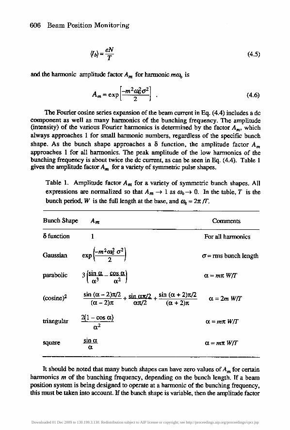
The Fourier cosine series expansion of the beam current in Eq. (4.4) includes a de component as well as many harmonics of the bunching frequency. The amplitude (intensity) of the various Fourier harmonics is determined by the factor A m , which always approaches 1 for small harmonic numbers, regardless of the specific bunch shape. As the bunch shape approaches a 5 function, the amplitude factor A m

approaches 1 for all harmonics. The peak amplitude of the low harmonics of the bunching frequency is about twice the de current, as can be seen in Eq. (4.4). Table 1 gives the amplitude factor A m for a variety of symmetric pulse shapes.

Table 1. Amplitude factor Am for a variety of symmetric bunch shapes. All expressions are normalized so that Am --> 1 as 600---> 0. In the table, T is the

bunch period, W is the full length at the base, and oJ b = 2x/T.

Bunch Shape Am Comments

8 function 1 For all harmonics

Gaussian cxp [-m2_o~ or2) ff = rms bunch length 2

parabolic 3 [ sin ot _ cos ot I ot = m~ WIT a 3 a 2 ]

(cosine) 2 sin (r - 2)~/2 + sin r + sin (r + 2)~/2 r = 2m W/T (a - 2)n an~2 (a + 2)n

triangular 2(1 - cos or) a = mn W/T o~ 2

square ~in a a = mx WIT o~

It should be noted that many bunch shapes can have zero values o f A m for certain harmonics m of the bunching frequency, depending on the bunch length. If a beam position system is being designed to operate at a harmonic of the bunching frequency, this must be taken into account. If the bunch shape is variable, then the amplitude factor


R. E. Shafer 607

may vary and may even go to zero, depending on the specific bunch shape and length. In summary, the currents associated with periodically spaced beam bunches

may be considered in either the time domain or the frequency domain. Generally, if the signal processing is performed at harmonic m = 1 in the frequency domain, the amplitude factor A 1 is nearly 1, and the rms beam intensity at this frequency is ~/2 times the dc current.

In cases where there is no significant beam bunching, or the beam bunching frequency is inconvenient, it is possible to induce a small detectable signal by modulating the beam current at the source. This modulation may be very small relative to the total beam current. At CEBAF, a 1-gA rms beam current modulation at 10 MHz is placed on the 200-gA cw electron beaml0 (rf frequency is 1497 MHz). Because the 10-MHz modulation can be turned on for less than one revolution around the recirculating linac (period about 4.2 Its), it is possible to measure the position of individual orbits while the machine is in operation. This method has two advantages: (1) the instrumentation is less expensive at 10 MHz than at 1497 MHz, and (2) the modulation scheme can be used without adversely affecting running experiments.

If a beam is centered in a circular, conducting beam pipe of radius b and has a velocity Vb = fib c (where c is the speed of ligh0, then there is an electromagnetic field accompanying the beam and an equal magnitude, opposite charge, uniformly- distributed beam current density on the inner wall of the beam pipe. The field inside the beam pipe looks (nearly) like a transverse-electric-magnetic (TEM) wave propagating down the beam pipe at the beam velocity (this is exact only for fit, = 1). Beam position detectors sense these fields (or equivalently the corresponding wall current) and determine the beam position based on the relative amplitudes of the induced signals in two or more pickup electrodes. The instantaneous Fourier harmonic amplitudes of the wall currents (integrated over 2~) in this case are the same as those for the beam itself.

The wall current density for a centered beam is then, for a beam pipe with inf'mite conductivity, simply the beam current divided by the beam-pipe circumference:

i w ( t ) = [ ~ ] (4.7)

Some authors like to differentiate between pickups that detect the TEM fields and those that sense the wall currents. There is no difference. For a beam current Ib(0 in the center of a conducting beam pipe of radius b, the azimuthal magnetic field accompanying it is Ho(r,t) = Ib(t)[27rr. Because [curl H(t)]z = Jz(t), the discontinuity of Ho(r,O at r = b requires that Jz(b,t) = Ho(b,t), as long as the magnetic fields associated with the beam are confined to the region inside the beam pipe. For this reason, we can consider either the TEM wave or the wall current density as the excitation signal. For an if-modulated cw beam in a metallic beam pipe, the magnetic field associated with the de component of Eq. (4.4) will eventually appear outside the beam pipe, and the wall currents will then include only the ac components.

As circular beam pipes are the most common shape, the rest of this paper will deal exclusively with circular geometry. Other geometries for beam pipes and beam pickup electrodes include rectangular, diamond, and elliptical, among others. All the



calculations carried out in this paper can be done for these other geometries, with similar results.

5 SIGNALS FROM OFF-CENTER BEAMS In the preceding section, we considered a centered beam in a circular beam pipe.

We now investigate what happens to the wall currents when the beam is displaced from the center.

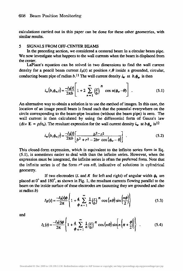
LaPlace's equation can be solved in two dimensions to find the wall current density for a pencil beam current Ib(t) at position r,O inside a grounded, circular,

conducting beam pipe of radius b. 11 The wall current density iw at b, cAr is then

iwb,~,t=( ) 1 + 2 Y~ cos n (~ -O) . (5.1) n--1

An alternative way to obtain a solution is to use the method of images. In this case, the location of an image pencil beam is found such that the potential everywhere on the circle corresponding to the beam-pipe location (without the beam pipe) is zero. The wall current is then calculated by using the differential form of Gauss's law (div E = p/go). The resultant expression for the wall current density i~, at bow isl2

= -1b(O [ b2- : ] iw(b,~,') 2~b Lb 2 +r2_2br c o s ( ~ - O )

(5.2)

This closed-form expression, which is equivalent to the infinite series form in Eq. (5.1), is sometimes easier to deal with than the infinite series. However, when the expression must be integrated, the infinite series is often the preferred form. Note that the infinite series is of the form rn cos nO, indicative of solutions in cylindrical geometry.

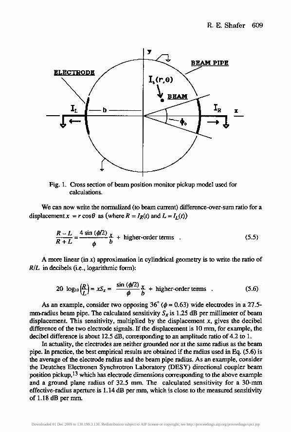
If two electrodes (L and R for left and right) of angular width O0 are placed at 0 ~ and 180 ~ as shown in Fig. I, the resultant currents flowing parallel to the beam on the inside surface of these electrodes are (assuming they are grounded and also at radius b)

cos(.o) IR(t)= . 1 ~ =

and

l~n=l n (nO}si~ {z+~}]} . c o s n (5.4)


R. E. Sh a f e r 609

B E A M PIPE

Fig. 1. Cross section of beam position monitor pickup model used for calculations.

We can now write the normalized (to beam curren0 difference-over-sum ratio for a displacement x = r cos0 as (where R = IR(t) and L = IL(t))

R - L = 4 sin (~r2) x + higher-order terms (5.5) R + L tp b

A more linear (in x) approximation in cylindrical geometry is to write the ratio of RIL in decibels (i.e., logarithmic form):

sin (~2) 20 log10 [-~ = xSx - ~ + higher-order terms (5.6)

r b

As an example, consider two opposing 36 ~ (q~ = 0.63) wide electrodes in a 27.5- mn~adius beam pipe. The calculated sensitivity Sx is 1.25 dB per millimeter of beam displacement. This sensitivity, multiplied by the displacement x, gives the decibel difference of the two electrode signals. If the displacement is 10 mm, for example, the decibel difference is about 12.5 riB, corresponding to an amplitude ratio of 4.2 to 1.

In actuality, the electrodes arc neither grounded nor at the same radius as the beam pipe. In practice, the best empirical results arc obtained if the radius used in Eq. (5.6) is the average of the electrode radius and the beam pipe radius. As an example, consider the Dcutches Electronen Synchrotron Laboratory (DESY) directional coupler beam position pickup, 13 which has electrode dimensions corresponding to the above example and a ground plane radius of 32.5 mm. The calculated sensitivity for a 30-mm effective-radius aperture is 1.14 dB per mm, which is close to the mcasurod sensitivity of 1.18 dB per mm.



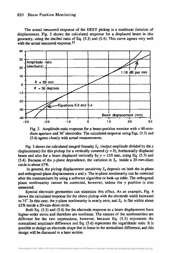
The actual measured response of the DESY pickup is a nonlinear function of displacement. Fig. 2 shows the calculated response for a displaced beam in this geometry, using the decibel ratio of Eq. (5.3) and (5.4). This curve agrees very well with the actual measured response. 13

4 0 .

3 0 - Amplitude ratio

20- (decibels)...

10

-10

-20

-30

-40 - 3 0

/ .18 dB per mm

b = 3 0 m m

r = 3 6 d e g r e e s

~ , , , ~ ~ . , . . . . - - E q u a t i o n s 5 .3 and 5 .4

�9 . . Beam disp!acement (mm)

-20 - 1 0 0 10 2 0 3 0

Fig. 2. Amplitude-ratio response for a beam-position monitor with a 60-rnm- diam aperture and 36" electrodes. The calculated response using Eqs. (5.3) and (5.4) agrees closely with actual measurements.

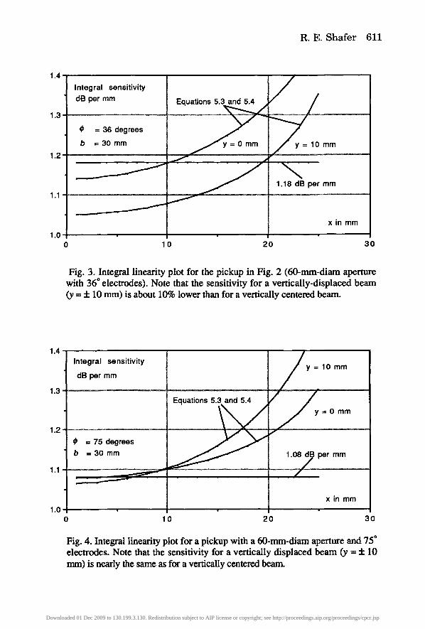
Fig. 3 shows the calculated integral linearity Sx (output amplitude divided by the x displacemen0 for this pickup for a vertically centered (y = 0), horizontally displaced beam and also for a beam displaced vertically by y = +10 mm, using Eq. (5.3) and (5.4). Because of the y-plane dependence, the variation in Sx inside a 20-mm-diam circle is about 5:7%.

In general, the pickup displacement sensitivity Sx depends on both the in-plane and orthogonal-plane displacements x and y. The in-plane nonlinearity can be corrected after the measurement by using a software algorithm or look-up table. The orthogonal plane nonlinearity cannot be corrected, however, unless the y position is also measured.

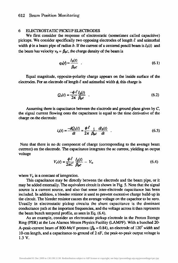
Special electrode geometries can minimize this effect. As an example, Fig. 4 shows the calculated response for the above pickup with the electrode width increased to 75 ~ In this case, the y-plane nonlinearity is nearly zero, and Sx is fiat within about +9% inside a 20-mm-diam circle.

Both Eq. (5.5) and (5.6) for the electrode response to a beam displacement have higher-order terms and therefore are nonlinear. The natures of the nonlinearities are different for the two expressions, however, because Eq. (5.5) represents the normalized amplitude difference and Eq. (5.6) represents the logarithmic ratio. It is possible to design an electrode shape that is linear in the normalized difference, and this design will be discussed in a later section.


R. E. Shafer 611

1.4.

1.3.

1.2.

1.1

1.0 0

Integral sensitivity dB per mm

= 36 degrees

b = 30 mm

Equations 5.3 and 5.4 N-'---..../

--o mm

J/ ~ 1 0 mm

1.18 dB per mm

x in mm

0 20 30

Fig. 3. Integral linearity plot for the pickup in Fig. 2 (60-mm-diam aperture with 36 ~ electrodes). Note that the sensitivity for a vertically-displaced beam (y -- + 10 mm) is about 10% lower than for a vertically centered beam.

1.4

1.3

1.2 = 75 degrees

1.1 ~, ~ i

1.0. 0 0

Integral sensitivity

dB per mm

b

Equations 5.3 and 5.4 /

[__

= 30 mm J J

2O

y = 10 mm

~ y = O mm

1.08 dE} per mm /

/

x in mm

30

Fig. 4. Integral linearity plot for a pickup with a 60-mm-diam aperture and 75* electrodes. Note that the sensitivity for a vertically displaced beam (y = + 10 mm) is nearly the same as for a vertically centered beam.



6 ELECTROSTATIC PICKUP ELECTRODES We first consider the response of electrostatic (sometimes called capacitive)

pickups. We consider specifically two opposing electrodes of length e and azimuthal width ~ in a beam pipe of radius b. If the current of a centered pencil beam is Ib(t) and the beam has velocity vb = flbC, the charge density of the beam is

qb(t) = lb(t) (6.1) #bC

Equal magnitude, opposite-polarity charge appears on the inside surface of the electrodes. For an electrode of length ~ and azimuthal width ~, this charge is

Q s ( t ) = -'0 g lb(t) (6.2) 2~ #bc

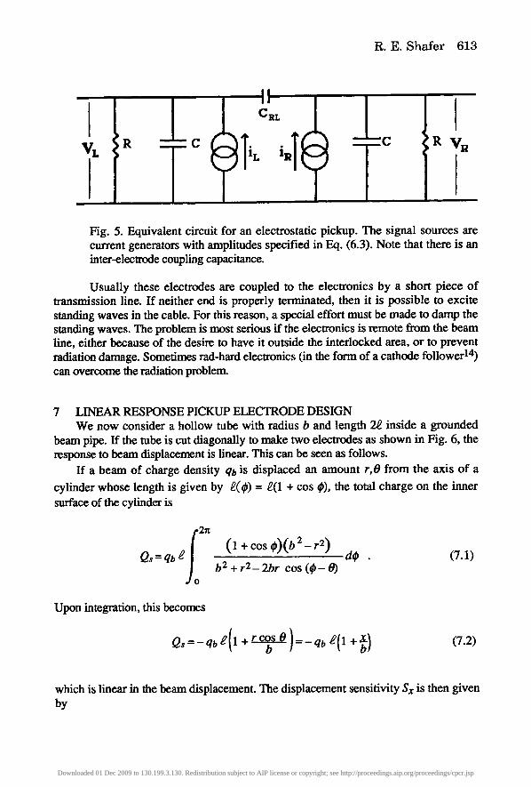
Assuming there is capacitance between the electrode and ground plane given by C, the signal current flowing onto the capacitance is equal to the time derivative of the charge on the electrode:

--dQs(t) Cg 1 d/b(t) (6.3) is(t)= dt =2Z flbC dt

Note that there is no dc component of charge (corresponding to the average beam cutrrent) on the electrode. The capacitance integrates the ac current, yielding an output voltage

Vc(t) = ~----(-~ lb(t) Vo (6.4) 2gC file

where V0 is a constant of integration. This capacitance may be directly between the electrode and the beam pipe, or it

may be added externally. The equivalent circuit is shown in Fig. 5. Note that the signal source is a current source, and also that some inter-electrode capacitance has been included. In addition, a bleeder resistor is used to prevent excessive charge build-up in the circuit. The bleeder resistor causes the average voltage on the capacitor to be zero. Usually in electrostatic pickup circuits the shunt capacitance is the dominant conductance path at the important frequencies, and the voltage across it then represents the beam bunch temporal profile, as seen in Eq. (6.4).

As an example, consider an electrostatic pickup electrode in the Proton Storage Ring (PSR) at the Los Alamos Meson Physics Facility (LAMPF). With a bunched 20- A-peak-current beam of 800-MeV protons (fib = 0.84), an electrode of 120 ~ width and 10-cm length, and a capacitance-to-ground of 2 nF, the peak-to-peak output voltage is 1.3 V.


R. E. S h a f e r 613

R c �9 C R I

VR

J Fig. 5. Equivalent circuit for an electrostatic pickup. The signal sources are current generators with amplitudes specified in Eq. (6.3). Note that there is an inter-electrode coupling capacitance.

Usually these electrodes are coupled to the electronics by a short piece of transmission line. If neither end is properly terminated, then it is possible to excite standing waves in the cable. For this reason, a special effort must be made to damp the standing waves. The problem is most serious if the electronics is remote from the beam line, either because of the desire to have it outside the interlocked area, or to prevent radiation damage. Sometimes rad-hard electronics (in the form of a cathode follower 14) can overcome the radiation problem.

7 LINEAR RESPONSE PICKUP ELECTRODE DESIGN We now consider a hollow tube with radius b and length 22 inside a grounded

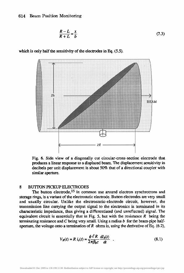
beam pipe. If the tube is cut diagonally to make two electrodes as shown in Fig. 6, the response to beam displacement is linear. This can be seen as follows.

If a beam of charge density q# is displaced an amount r, 0 from the axis of a

cylinder whose length is given by g(r = g(1 + cos ~), the total charge on the inner surface of the cylinder is

Qs = qb s

J O

(1 + cos 2_ , 9 b 2 + r 2 - 2br cos ( r O)

d~ . (7.1)

Upon integration, this becomes

(7.2)

which is linear in the beam displacement. The displacement sensitivity Sx is then given by



R - L x = - - ( 7 . 3 )

R + L b

which is only half the sensitivity of the electrodes in Eq. (5.5).

Fig. 6. Side view of a diagonally cut circular-cross-section electrode that produces a linear response to a displaced beam. The displacement sensitivity in decibels per unit displacement is about 50% that of a directional coupler with similar aperture.

8 BUTION PICKUP ELECTRODES The button electrode, 15 in common use around electron synchrotrons and

storage rings, is a variant of the electrostatic electrode. Button electrodes are very small and usually circular. Unlike the electrostatic-electrode circuit, however, the transmission line carrying the output signal to the electronics is terminated in its characteristic impedance, thus giving a differentiated (and unreflected) signal. The equivalent circuit is essentially that in Fig. 5, but with the resistance R being the tem-,inating resistance and C being very small. Using a radius b for the beam-pipe half- aperture, the voltage onto a termination of R ohms is, using the derivative of Eq. (6.2),

c~gR dlb(O (8.1) VR(O = R is(O = 2x&c at


R. E. Shafer 615

For circular electrodes, the factor ~ eb in the equation should be set equal to the electrode area.

It is useful to combine Eq. (8.1) with Eq. (4.1) to calculate the button-electrode

response to a single Gaussian beam bunch containing N particles (for o'> e/flbC):

-eN ~ gR 1_ exp VR(t) (2~)3/2 flbC O 3

(8.2)

The peak output voltage of this bipolar doublet, which occurs at about t = +o', is then given by

Vpea k _-- -4- cN ~ ~ g e-m (8.3) 3/2 & c a 2

This peak amplitude varies inversely as the square of the beam bunch length. For this reason, button electrodes are most useful around machines with very short bunches (i.e. electron accelerators and storage rings) and are not normally used around proton machines, which typically have longer bunch lengths (an exception to this is the PETRA ring at DESY, which will use button electrodes for monitoring both electron and proton beams).

If we use Eq. (8.1) in combination with the Fourier series expression as shown in Eq. (4.4), the rms output voltage for a beam intensity signal at frequency af2x is

VR (r = r ~b)A(o~) tag (8.4) X 2flbC

where A(og) is the amplitude factor Eq. (4.6) at frequency to/2x. This signal amplitude

rises linearly with ogfor a given average beam current when or> ~/flbC.

9 RESONANCES IN PICKUP ELECTRODES We now consider a simple electrostatic electrode inside the beam pipe, as shown in

Fig. 7. Assuming the only external connection to the electrode is at the center, both the upstream and downstream ends of the electrode are open (i.e., unterminated). Because the electrode forms a transmission line with the beam pipe wall behind it and has a capacitance and an inductance per unit length, the electrode can resonate with current nodes at each end. Any resonance that has a voltage node at the external connection will resonate with a high Q, because no power can be coupled into the external circuit. The voltage induced by the passing beam thus remains on the electrode and, in some instances, can lead to beam instabilities. For this reason, electrostatic-type pickups of any shape should be avoided if possible. An exception is the button electrode, which is so short that the resonances are at very high frequencies (tens of GHz).



One way to couple to all the resonances in pickups is to make the external signal attachment at one end. In this way all resonances will couple to the external circuit. If, however, the transmission line used for the external circuit has a different characteristic impedance than the electrode itself, there will be a voltage-standing-wave ratio (VSWR) at the connection, and several reflections will be required for the power on the electrode to escape onto the transmission line. This will distort the temporal response of the electrode, which is a concern if the electrode is to be used at high frequencies. In some instances, this feature could be used as an aid to signal processing by creating a pulse train from isolated single beam bunches.

The standard solution for minimizing the VSWR is to match the characteristic impedance of the electrode and the transmission line. In this case, the power induced on the electrode is transferred to the transmission line without any reflection and therefore appears immediately in the external circuit. This design is discussed in the following section.

Fig. 7. Side view of an electrostatic pickup with the signal connection at the center. Because both ends are unterminated, the beam can excite high-Q resonances in the electrode that have current nodes at the ends and a voltage node at the center.

10 DIRECTIONAL COUPLER PICKUP ELECTRODES Directional coupler pickup electrodes (sometimes referred to as "stripline" or

"microstrip" electrodes) are essentially transmission lines with a well-defined characteristic impedance and with a segment of the center conductor exposed to the beam.

We will examine the signal formation on this type of electrode in both the time and frequency domains. First, we consider the time domain.

Consider an electrode of azimuthal width r length ~, and characteristic impedance Z in a cylindrical beam pipe of radius b, as shown in Fig. 8. If the beam current is

Ib(t), the wall current intercepted by the electrode is -(~12z) �9 Ib(t) for a centered beam. This is the current that flows on the inner surface of the electrode exposed to the beam.


R. E. Shafer 617

When the beam pulse approaches the upstream end of the electrode, this wall current must cross the gap from the beam pipe wall to the electrode. Because the impedance of the gap is half the electrode's characteristic impedance (the inducing current sees two transmission lines in parallel), the voltage induced across the gap is V(t) = ( r (Z/2)- Ib(t). This voltage then launches TEM waves in two directions. One signal goes out the upstream port to the electronics. The other wave travels down the outside surface (the surface facing the beam pipe) of the electrode to the downstream port at a signal velocity vs = ~sc and out the downstream port. Because the impedance of the transmission line is Z, the current flowing in each direction is half the current flowing on the inside surface (facing the beam) of the electrode. The beam and the image signal on the inside surface travel down the beam pipe at a velocity vb = ~bC and induce a similar signal at the downstream port, with a

delay given by g/Jibe and with opposite polarity to the first one. The net result is that at the upstream port we see a bipolar-doublet signal of the form

(10.1)

while at the downstream port, the bipolar signal is given by

VD (O = e'Z l-- lb l , - - - -&l (10.2)

COAX

Ill N-

I i g I

I I

I I

, / V

COAX

COAX

BEAIdPIPE [_LI

ELECTRODE \

b I BEAM I

71 COAX

I /

.#

Fig. 8. Side view of a directional-coupler beam position electrode. The electrode is a section of a matched transmission line with the center electrode exposed to the image fields of the passing beam. Signals induced on the electrode exit through the upstream and downstream ports without reflection.



If/~bC equals the TEM wave velocity/~sC on the electrode, there is complete signal cancellation at the downstream port. This form of electrode structure therefore can be highly directional. Directivities (the ratio of forward to reverse power) close to 40 dB have been obtained. This is quite useful in monitoring beams in collider-type storage rings that have counter-rotating beams.

This geometry has several variations. In addition to terminating the downstream port in the characteristic impedance, the port may be either shorted to ground or left open. In these cases, the signal traveling down the electrode to the downstream port is reflected, either inverted (shorted electrode) or non-inverted (open electrode). In the latter case, a signal induced at the downstream port by the beam has twice the amplitude of the reflected signal and the opposite polarity. In all cases, the output signal at the upstream port is a bipolar doublet with zero net area.

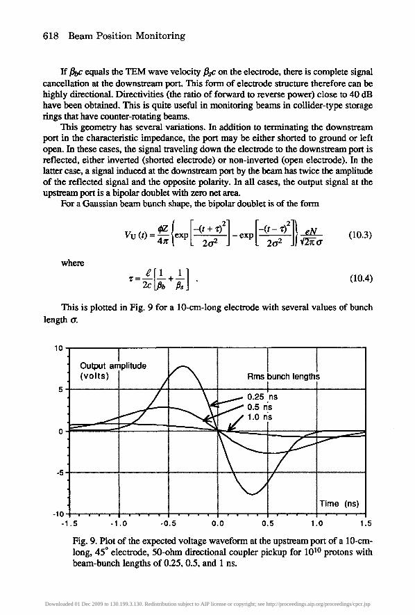
For a Gaussian beam bunch shape, the bipolar doublet is of the form

/ox F ,:+el ox I ,' 4 z | L 2o -2 J L 2o .2 J/~-~-O"

(lO.3)

where

~r=~ + . (10.4)

This is plotted in Fig. 9 for a 10-cm-long electrode with several values of bunch length G.

10

5

f o

-5

-10 . . . . -1.5

Output amplitude / ~ (volts) /

.0 -0.5

Rms bunch lengths l

0.25 'ns . ~ 0 . 5 n's

1.0 n's

L

i Time (ns) �9 �9 , �9 �9 . . . . . . .

0.0 0.5 1.0 1.5

Fig. 9. Plot of the expected voltage waveform at the upstream port of a 10-cm- long, 45* electrode, 50-ohm directional coupler pickup for 101~ protons with beam-bunch lengths of 0.25, 0.5, and 1 ns.


R. E. Shafer 619

The same analysis can be performed in the frequency domain using Eq. (4.4) for a beam current modulated at frequency o~2x. In this case the rms voltage at the upstream port is

Vo(w)=~--~b)a(c~ ~fls fib (10.5)

and the rms voltage at the downstream port is

VD(O~)=~----~qb)A(o~)sin[~[1--~)] 'fls (10.6)

Note that there is an electrode of such a length that the argument of the sine function in Eq. (10.5) is x/2, and the output signal is maximized. This electrode is sometimes referred to as a "quarter wavelength" electrode, even though it is not quite quarter wavelength except when fib and fls are both equal to 1. Note also that the response function contains periodic zeros when the argument is equal to nx. When this type of pickup is used as a wide-band pickup for looking at signals over a large frequency range, these dips in the response function are easily observed.

At low frequencies, the circular function in the expression for the signal amplitude at the upstream port can be replaced by its argument. The rms output voltage at low frequencies then becomes (co = mo~)

(10.7)

This approximation is valid if the electrode is substantially shorter than a quarter wavelength.

Comparing this approximation to Eq. (8.4) for the button electrode, we see that the two expressions are identical if the signal velocity fls in Eq. (10.7) is set to infinity and R in Eq. (8.4) is set to Z/2. We have used two very different electrode designs in these calculations and two very different calculational methods. When a directional coupler electrode is very short, the output impedance does look like ZI2 (because it is terminated in Z at both ends), and we can also ignore the finite signal velocity on the electrode; therefore this equivalence is expected.

11 OTHER TYPES OF ELECTROMAGNETIC PICKUPS Several other types of electromagnetic position pickups should be mentioned.

Small loop couplers 16 (often called B-dot loops, meaning dBIdt) are simply small shorted antennas that couple to the azimuthal magnetic field of the passing beam and can be quite directional.

A second type of position pickup used in the past is the "window-frame" (or magnetic) pickup electrode. 17 In this design, a ferrite window frame is linked with a



conductor so that off-center beams create a difference signal. The frequency response of this type of pickup is limited by the magnetic properties of the ferrite.

A third type is the so-called slot coupler (Faltin pickupl8), in which the beam fields couple to a nearby center conductor of a transmission line through holes or slots in the ground-plane wall and induce signals that travel in both directions on the transmission line, the forward one being coherent. One shortcoming of this design is that the slots make the transmission line dispersive, and the signal remains in synchronism with the beam for only a short distance. A multi-slot version of this pickup produces a pulse- train signal at the upstream port for single isolated beam bunches. This feature can be an aid to signal processing. 19

A fourth type is a resonant rf cavity excited by a bunched beam in a TM mode that has a null for a centered beam. An off-center beam excites cavity resonances whose amplitudes are proportional to the product of beam intensity and beam displacement, and whose phase depends on the direction of displacement. 20 Because rf cavities are high-Q, these cavities have a very narrow bandwidth. Because the signal amplitude is un-normalized (i.e., proportional to the beam current as well as to the displacemen0, the position can be determined only by referencing the signal to another signal that is proportional only to beam current. In certain applications, however, an un-normalized signal is adequate.

Last, an exponentially tapered stripline pickup, in which both the electrode width and its spacing from the beam pipe wall are exponentially tapered so as to maintain a constant impedance, was developed at CERN. 14 Its frequency response differs from that of the normal stripline pickup in that the periodic zeros predicted by Eq. (10.5) are not present.

12 BEAM SYNCHRONOUS PHASE MEASUREMENTS The phase of the beam rf structure relative to an rf cavity phase, or to a beam

phase measurement at another location, is often of considerable importance. In commissioning proton linear accelerators, the relative phases of the beam structure and the rf cavity voltage determine not only the accelerating gradient but also the longitudinal focusing field. Delta-t measurements 21 are used to set proton linac cavity amplitude and phase. For non-relativistic beams, time-of-flight determination using phase measurement can be an effective method to determine energy.

The electrode geometry that provides the best phase response is the directional coupler geometry discussed in Section 10, because the design has minimized the possibility of reflections at impedance mismatches. Following the results of Eq. (10.1) for the signal at the upstream port of an electrode of length ~, we can write the amplitude of the component at frequency a/27r using phasor notation as

Vu(co, t) - o ~ - L - (12.1)

where k b = to/flbc and k s = adflsc for the beam and signal wave numbers respectively. We then may write the voltage seen at the upstream port as


R. E. Shafer 621

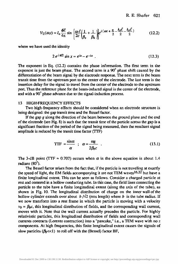
ez [o~e [ l+ l~ ] (o,t ~__k,g kse) V u ( tO, t) = Io ~ sin ~]e i + (12.2)

where we have used the identity

2 e i r'12 s i n x = e i x - e - i x . (12.3)

The exponent in Eq. (12.2) contains the phase information. The first term in the exponent is just the beam phase. The second term is a 90* phase shift caused by the differentiation of the beam signal by the electrode response. The next term is the beam transit time from the upstream port to the center of the electrode. The last term is the insertion delay for the signal to travel from the center of the electrode to the upstream port. Thus the reference plane for the beam-induced signal is the center of the electrode, and with a 90* phase advance due to the signal-induction process.

13 HIGH-FREQUENCY EFFECTS Two high-frequency effects should be considered when an electrode structure is

being designed: the gap transit time and the Bessel factor. If the gap g along the direction of the beam between the ground plane and the end

of the electrode (see Fig. 8) is such that the transit time of the particle across the gap is a significant fraction of the period of the signal being measured, then the resultant signal amplitude is reduced by the transit time factor (TIT)

sintx tog T r F - ; a - (13.1)

a 2/~bc

The 3-dB point (TTF = 0.707) occurs when oc in the above equation is about 1.4 radians (80~

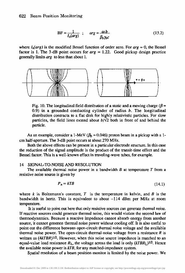
The Bessel factor arises from the fact that, if the particle is not traveling at exactly the speed of light, the EM fields accompanying it are not TEM wavesl6, 22 but have a finite longitudinal extent. This can be seen as follows. Consider a charged particle at rest and centered in a hollow conducting tube. In this case, the field lines connecting the particle to the tube have a finite longitudinal extent (along the axis of the tube), as shown in Fig. 10. The longitudinal distribution of charge on the inner wall of the hollow cylinder extends over about b/~/2 (rms length) where b is the tube radius. If we now transform into a rest frame in which the particle is moving with a velocity Vb = fibC, this longitudinal distribution of fields, and the corresponding wall current, moves with it. Note that the wall current actually precedes the particle. For highly relativistic particles, this longitudinal distribution of fields and corresponding wall currents contracts (Lorentz contraction) into a "pancake," i.e., a TEM wave with no z components. At high frequencies, this finite longitudinal extent causes the signals of slow particles (flb<<l) to roll off with the (Bessel) factor BF,


622 B e a m Pos i t ion M o n i t o r i n g

B F = 1 ; arg= rob (13.2) to(arg) 3b rbc

where Io(arg) is the modified Bessel function of order zero. For arg = 0, the Bessel factor is 1. The 3-dB point occurs for arg = 1.22. Good pickup design practice generally limits arg to less than about 1.

I I I ' 1 V Y d

Fig. 10. The longitudinal field distribution of a static and a moving charge (fl = 0.9) in a grounded conducting cylinder of radius b. The longitudinal distribution contracts to a flat disk for highly relativistic particles. For slow particles, the field lines extend about b/~2 both in front of and behind the particle.

As an example, consider a 1-MeV (fib = 0.046) proton beam in a pickup with a 1- cm half-aperture. The 3-dB point occurs at about 270 MHz.

Both the above effects can be present in a particular electrode structure. In this case the reduction of the signal amplitude is the product of the transit-time effect and the Bessel factor. This is a well-known effect in traveling-wave tubes, for example.

14 SIGNAL-TO-NOISE AND RESOLUTION The available thermal noise power in a bandwidth B at temperature T from a

resistive noise source is given by

Pn = kTB (14.1)

where k is Boltzmann's constant, T is the temperature in kelvin, and B is the bandwidth in hertz. This is equivalent to about - 1 1 4 dBm per MHz at room temperature.

It is useful to point out here that only resistive sources can generate thermal noise. If reactive sources could generate thermal noise, this would violate the second law of thermodynamics. Because a reactive impedance cannot absorb energy from another source, it cannot generate thermal noise power without cooling off. It is also useful to point out the difference between open-circuit thermal noise voltage and the available thermal noise power. The open-circuit thermal-noise voltage from a resistance R is written as (4kTBR) lt2. However, when this noise source impedance is matched to an equal-value load resistance RL, the voltage across the load is only (kTBRL) lt2. Hence the available noise power is kTB, for any matched-impedance system.

Spatial resolution of a beam position monitor is limited by the noise power. We


R. E. Shafer 623

can use the relations developed in Eq. (5.5) or (5.6) to estimate the resolution limit due to thermal noise. The resolution limit is

Sx_ ~ A/-P-~ ~- IA f / ~ (14.2) b 8sin(0/2) V Ps 4 V Ps

where Ps is the signal power on a single electrode, and Pn is the noise power. Here we

have used the thermal noise variance O'n2 =Pn/2. Hence a 40-dB signal-to-noise ratio (100:1 amplitude ratio) limits the resolution to about 0.25% of the half aperture.

As an example, consider a 1-mA beam in a quarter-wavelength, 45 ~ (0=0.79 radian), 50-ohm pickup. The signal power Ps per electrode at the upstream port of a directional coupler is given by

Ps = 2 Z ~lb} 2 A 2(09) sin 2 [aZ__g [ 1_2__ + 1 / ] [2c (14.3)

With the above parameters, Ps = 1.56 gW, which corresponds to -28 dBm. With a 10-MHz bandwidth and an electronic noise figure of 6 dB, the noise power Pn is -98 dBm. Thus the signal-to-noise ratio is about 70 dB, and the resolution limit is about 3 grn for a 50-mm-diam aperture.

It is straightforward to estimate the thermal phase noise on a signal if the signal and noise power are known. Because the thermal noise phasor represents a circle on the tip of the signal phasor, we can write for the thermal phase noise

(14.4)

This is important when the signal phase is being used for determining the phase of an rf cavity or for making time-of-flight energy measurements.

Note in Eq. (14.3) that the signal power scales linearly with the characteristic impedance of the pickup, as is expected for current sources. Thus if signal-to-noise is a problem, raising the pickup impedance is a solution. Broad-band (non-resonant) pickups with impedances >100 ohms have been used successfully. One way to accomplish this over a narrow band is to use a quarter-wave (transmission line) transformer at the pickup to match the pickup to the cable. Resonant beam position pickups with effective electrode input impedances of -- 5000 ohms have been made to measure the position of very small beam currents. 23

The RFI from accelerator rf systems can have serious effects on the accuracy and resolution if the shielding is not adequate. If the beam-bunching frequency is a subharmonic of the rf frequency, then operating the pickup at the lower frequency often eliminates the interference. If the beam is bunched at the rf frequency, then operating the pickup at a higher harmonic will eliminate the rf interference. EMI (electromagnetic interference) from pulsed and SCR power supplies is often a problem, and great care must be taken to eliminate ground loops that can pick up noise.



Shot noise is not a noise in the case of particle beams, but a signal. It relates specifically to fluctuations in the instantaneous beam current caused by the granularity of the individual particle charges. Because the fluctuations in beam current create a carrier signal, they allow detection of the beam position and therefore are sometimes called Schottky currents. The rms Schottky current for a coasting beam of average current <Ib> and bandwidth B is (for particles with charge :t:e)

lshot= (2eqb) B) in (14.5)

A specific example is that the Schottky current for a 1-A proton beam with a 1- MHz bandwidth is 0.6 gA.

15 BEAM COUPLING IMPEDANCE An important parameter in the design and construction of circular machines is the

coupling impedance of beam line components. Most beam line components, including steps in the size of the beam pipe, resistive beam-pipe walls, rf cavities, kicker magnets, and beam diagnostics couple to the beam. Specifically, the beam current creates a complex voltage (i.e., with both real and reactive components) across the device as the beam passes by. This beam-induced voltage then reacts back onto the beam. The voltage may be either longitudinal (Ez), or transverse (E x or Ey). The ratio

of the induced rms voltage to the rms beam current at frequency co is referred to as the

beam coupling impedance Z(CO) = Re Z(co) + j Im Z(co). Because excessive beam coupling impedance can lead to beam instabilities, limits are placed on allowed longitudinal and transverse coupling impedances in circular machines.

It is straightforward to calculate the complex longitudinal coupling impedance of a directional-coupler (stripline) pickup. The power coupled from the beam at frequency co is given by Eq. (14.3). Thus the real part of the coupling impedance for a pair of electrodes is

2P(CO) _ 2 Z A2(CO) [sin 2 (arg 1) + sin 2 (arg 2)] (15.1) Re Z(co) =

where the frequency co = ncoo is expressed as a harmonic of the revolution frequency

oh/2x in a circular machine, and where

arg 1 = c o s + _ ~ (15.2) 2c abl

and arg 2 - cog[ 1 1 I (15.3) -wl -gJ

In Eq. (15.1), the two terms result from the fact that power is absorbed from the beam at both the upstream and downstream pickup ports unless the beam velocity and the


R. E. Shafer 625

signal velocity are equal. For low-energy proton accelerators where/~b is substantially less than 1, the second term is important.

Because the impedance is an analytic function and must satisfy the Kramers- Kronig relations, 24 the imaginary part of the complex impedance can be derived from the real part, yielding

2

ImZ(r Z A2(~) [sin (arl 1)cos(arg 1) + sin (ar12) cos (ars 2) ] (15.4)

The standard format for writing the longitudinal coupling impedance is to write the imaginary component at frequency o~ = nt00, divided by the harmonic number n:

Im Z(c.O)n ZL(~)n = n Z A2(~) [sin (arg 1) cos (arg 1) + sin (arg 2) cos (arg 2)] .

(15.5) It is interesting to note that this reactive coupling impedance fluctuates between inductive (the low-frequency limit) and capacitive. Transmission-line measurements on stripline pickups with wires confirm this effect. 25 The low-frequency limit for a single pair of electrodes is then [where 2rtR is the machine circumference and A(o~) =1]

ZL(0')) n = 2 Z ~ C ~--2Z R ~ , 05.6)

The magnitudes of Eq. (15.5) and (15.6) should be multiplied by 2 for four-electrode pickups. The transverse beam coupling impedance is then given by 11

2 . ZT(09) = ~ - C--if--] (15.7)

where b is the beam pipe radius.

16 THE EFFECT OF ATIENUATION AND DISPERSION IN CABLES In the frequency range encountered in the processing of beam position signals, the

single most important contributor to signal attenuation in cables is the skin-effect loss in the conductors. Dielectric losses become important only at microwave frequencies. The skin-effect attenuation per unit length for a coaxial cable of outer radius b, inner radius a, effective relative dielectric constant e, frequency f, and conductor volume resistivity

p is given by 26 (a neper is 8.686 decibels)

I : l . . l_l 1 nepers per meter (16.i) ln(b/a)



where the characteristic impedance and signal velocity are

Z = ~ In (b/a) , fls = 1N-~ (16.2)

Here c is the velocity of light and ~ is the permeability of free space. For copper, the volume-resistivity p is about 2 • 10 -8 ohm-meters. Thus for copper conductors Eq. (16.1) becomes (a and b are in meters)

ot = 3.63 x 10 -1~ + In (b/a) nepers per meter . (16.3)

Using Eqs. (16.1) and (16.2), it is straightforward to show that an air-dielectric coaxial transmission line with a fixed outer radius has minimum skin-effect attenuation when the characteristic impedance is 77 ohms for e = 1.

Note that the frequency dependence of the attenuation isflrz. Causality requires that if the signal attenuation in a 2-port passive system is known for all frequencies, then the phase shift is completely determined at all frequencies. This is another statement of the Kramers-Kronig relation used in the previous section. This effect is sometimes referred to as the real-part-sufficiency theorem in electrical engineering. For this case, where the attenuation frequency dependence isfl/2, the frequency-dependent phase shift, expressed in radians per meter, is numerically equal to the frequency- dependent attenuation, expressed in nepers per meter.

The convolution of the beam-pickup signal with the cable attenuation and dispersion may be expressed in the frequency domain by application of Parseval's theorem. Thus, if the bipolar output signal of a beam-position pickup can be written in the form [compare to Eq. (10.5)]

V(t)=~---(/b) ~ a(mo~o) sin ( ~ ) sin (moot) , (16.4) /[ m = l

then the complete expression for the attenuated beam-pickup-electrode signals, including both attenuation and dispersion, is

r ** Imo~ogl sin mogo[ (t_z) ~ V(t) = "-~-~b) Z exp(-amfmZ) A(m~ sin , ~ 1 (16.5) m= l

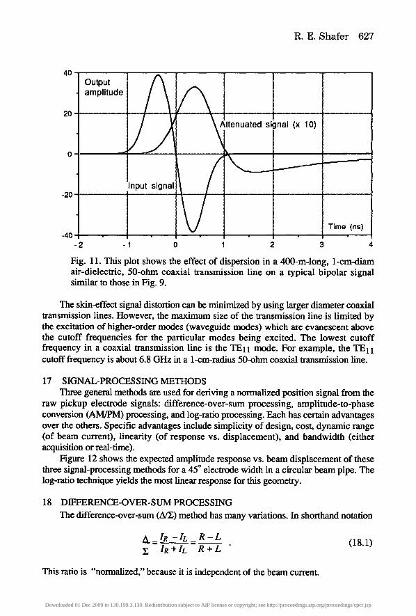
where (~m is the attenuation per unit length at frequency f = mo~0/2~, and x is the frequency-independent insertion delay for a lossless cable of length z. The distorted output signal V(t) (including attenuation and dispersion) is expressed in temporal form; i.e., a summation over the individual frequency components. The amplitudes of the individual frequency components are attenuated following the fl/2 rule, and their relative phases are skewed because of the frequency-dependent dispersion in the transmission line. An example of the distortion caused by the dispersion is shown in Fig. 11.


R. E. Shafer 627

40

20

-20

-40

Output amplitude

Input signali

V

~ ttenuated signal (x 10)

Time (ns)

3 4 2 -1 0 2

Fig. 11. This plot shows the effect of dispersion in a 400-mJong, 1-cm-diam air-dielectric, 50-ohm coaxial transmission line on a typical bipolar signal similar to those in Fig. 9.

The skin-effect signal distortion can be minimized by using larger diameter coaxial transmission lines. However, the maximum size of the transmission line is limited by the excitation of higher-order modes (waveguide modes) which are evanescent above the cutoff frequencies for the particular modes being excited. The lowest cutoff frequency in a coaxial transmission line is the TEll mode. For example, the TEll cutoff frequency is about 6.8 GHz in a 1-cm-radius 50-ohm coaxial transmission line.

17 SIGNAL-PROCESSING METHODS Three general methods are used for deriving a normalized position signal from the

raw pickup electrode signals: difference-over-sum processing, amplitude-to-phase conversion (AM/PM) processing, and log-ratio processing. Each has certain advantages over the others. Specific advantages include simplicity of design, cost, dynamic range (of beam current), linearity (of response vs. displacement), and bandwidth (either acquisition or real-time).

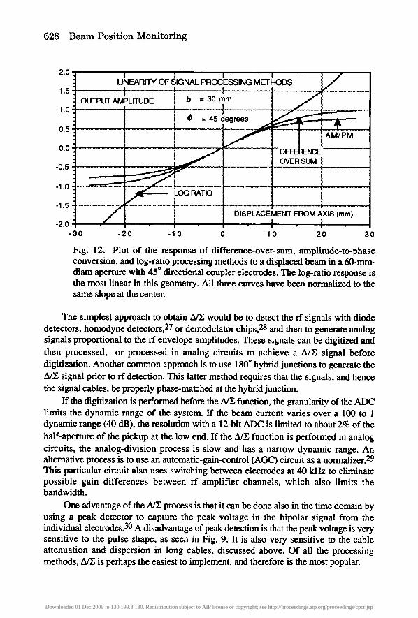
Figure 12 shows the expected amplitude response vs. beam displacement of these three signal-processing methods for a 45 ~ electrode width in a circular beam pipe. The log-ratio technique yields the most linear response for this geometry.

18 DIFFERENCE-OVER-SUM PROCESSING The difference-over-sum (A/Z) method has many variations. In shorthand notation

A _IR --1L _ R - L y, IR + IL R + L

(18.1)

This ratio is "normalized," because it is independent of the beam current.



2.0

1 .5

1 .0

0 . 5

0.0

- 0 . 5

-1.0

-1.5 1 -2.0

-30

! t ! J / UNEARITY OF SIGNAL PROCESSING METHODS

| b OUTPUT AMPLITUDE

, . - . . . . - . - , . . - - - ~

/

= 3 0 m m

t = 4 5 d e g r e e s

LOG RATIO

-20 -10

J DIH-~_NCE OVER SLIM

iiiiii AM/PM

it DISPLACEMENT FROM AXIS (ram)

�9 ] . ! .

0 1 0 2 0 3 0

Fig. 12. Plot of the response of difference-over-sum, amplitude-to-phase conversion, and log-ratio processing methods to a displaced beam in a 60-mm- diam aperture with 45* directional coupler electrodes. The log-ratio response is the most linear in this geometry. All three curves have been normalized to the same slope at the center.

The simplest approach to obtain A/Z would be to detect the rf signals with diode detectors, homodyne detectors, 27 or demodulator chips, 28 and then to generate analog signals proportional to the rf envelope amplitudes. These signals can be digitized and then processed, or processed in analog circuits to achieve a AlE signal before digitization. Another common approach is to use 180 ~ hybrid junctions to generate the A/Z signal prior to rf detection. This latter method re.quires that the signals, and hence the signal cables, be properly phase-matched at the hybrid junction.

If the digitization is performed before the A/Z function, the granularity of the ADC limits the dynamic range of the system. If the beam current varies over a 100 to 1 dynamic range (40 dB), the resolution with a 12-bit ADC is limited to about 2% of the half-aperture of the pickup at the low end. If the A/Z function is performed in analog circuits, the analog-division process is slow and has a narrow dynamic range. An alternative process is to use an automatic-gain-control (AGC) circuit as a normalizer. 29 This particular circuit also uses switching between electrodes at 40 kHz to eliminate possible gain differences between rf amplifier channels, which also limits the bandwidth.

One advantage of the A/Z process is that it can be done also in the time domain by using a peak detector to capture the peak voltage in the bipolar signal from the individual electrodes. 30 A disadvantage of peak detection is that the peak voltage is very sensitive to the pulse shape, as seen in Fig. 9. It is also very sensitive to the cable attenuation and dispersion in long cables, discussed above. Of all the processing methods, A/Z is perhaps the easiest to implement, and therefore is the most popular.


R. E. Shafer 629

19 AMPLITUDE-TO-PHASE-CONVERSION PROCESSING In the amplitude-modulation-to-phase-modulation (AM/PM) method,31,32 the two

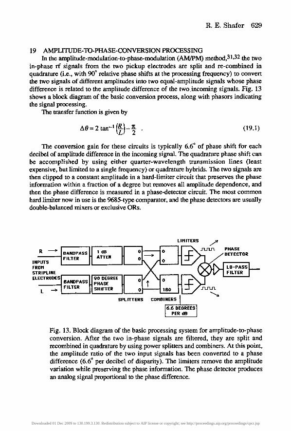
in-phase rf signals from the two pickup electrodes are split and re-combined in quadrature (i.e., with 90 ~ relative phase shifts at the processing frequency) to convert the two signals of different amplitudes into two equal-amplitude signals whose phase difference is related to the amplitude difference of the two incoming signals. Fig. 13 shows a block diagram of the basic conversion process, along with phasors indicating the signal processing.

The transfer function is given by

AO = 2 tall -1 IRI - ~ (19.1) 2 ' / . , !

The conversion gain for these circuits is typically 6.6 ~ of phase shift for each decibel of amplitude difference in the incoming signal. The quadrature phase shift can be accomplished by using either quarter-wavelength transmission lines (least expensive, but limited to a single frequency) or quadrature hybrids. The two signals are then clipped to a constant amplitude in a hard-limiter circuit that preserves the phase information within a fraction of a degree but removes all amplitude dependence, and then the phase difference is measured in a phase-detector circuit. The most common hard limiter now in use is the 9685-type comparator, and the phase detectors are usually double-balanced mixers or exclusive ORs.

INPUTS FROM STRIPLINE ELECTRODES

LIMITERS .,.,;4"

FILTERBANDPASSUII'T" o o

�9 ~ CO-PASS I ~ " ~ V I FILTER I

go DEGREE i zF'~;.ru.m ' IIANDPASS PHASE FILTER SHIFTER GO

L '-'> / SPLITTERS COMBINERS

6.6 DEGREES PER dB I

Fig. 13. Block diagram of the basic processing system for amplitude-to-phase conversion. After the two in-phase signals are filtered, they are split and recombined in quadrature by using power splitters and combiners. At this point, the amplitude ratio of the two input signals has been converted to a phase difference (6.6 ~ per decibel of disparity). The limiters remove the amplitude variation while preserving the phase information. The phase detector produces an analog signal proportional to the phase difference.



The analog voltage output of the AM/PM processor is related to the amplitudes R and L of the two input signals by the relation

R g _ I [ R - L ] V o . , = Vo t a n - " (19.2)

Note the relationship to the A/Z processing algorithm. The hard limiter is usually the component that most limits the system performance.

Their dynamic range varies from 40 to >60 dB depending on the operating frequency. They have been used at frequencies >100 MHz but perform best below about 20 MHz. To use hard limiters when the beam-current modulation is >100 MHz, the rf signal is often heterodyned down to a lower frequency, typically 10 or 20 MHz. The real-time bandwidth is about 10% of the processing frequency and can be as high as 10 MHz.

AM/PM circuits using down conversion from 200 to 10 MHz and 425 to 20 MHz have been built at Los Alamos. 33 Fermilab has built about five hundred 53-MHz units and has built down-conversion units for both the 200-MHz proton linac and the rapid- cycling Booster synchrotron. 34 This latter application is quite interesting in that the local oscillator used for the down conversion tracks the Booster rf frequency from 30 to 53 MI-Iz with a constant frequency offset, so that the IF frequency output to the AM/PM circuit is constant.

It is essential to keep the relative phases of the two signals entering the AM/PM processor within about +5", otherwise Eq. (19.1) must be modified. Phase matching of the cables from the pickups to the electronics is therefore required.

The AM/PM circuits are specifically well suited for frequency-domain signal processing and therefore function well for multi-bunch beam pulses. AM/PM processing has also been used to measure the position of single, isolated beam bunches. In this application, a narrow-band (or transversal) filter is placed upstream of the AM/PM processor. The passage of a single bunch by the pickup electrode shock- excites the filter to ring at a well-defined frequency for perhaps 10 cycles, which is sufficient time to complete the phase difference measurement. 32 These filters must be very carefully matched, with center frequencies equal within about s The reason for the tight matching requirements is that the relative phase error should not exceed about 5 ~ during the time the filter is ringing. Both lumped-component circuits and shorted coaxial transmission lines have been used in this application.

Real-time bandwidth is important if the signal is to be used in real-time control of the beam position. In this case, the processed beam position signals are fed back to beam deflector electrodes located upstream of the pickup, and the system is run in closed-loop fashion to reduce the transverse beam jitter. Because the AM/PM system provides a normalized position signal, the position signal is independent of beam intensity. The jitter-control function can be accomplished more simply by using an unnormalized difference signal if the beam intensity variation is minimal. In this case, the closed-loop gain is proportional to the beam intensity.

Of the three basic types of position processors reviewed here, the AM/PM circuit is the most expensive and difficult to implement. However, the obtainable large dynamic range and high real-time bandwidth are very desirable features. Thus far, their


R. E. Shafer 631

application is limited to the Linac, Booster, Main Ring, and Tevatron 35 at Fermilab; the Proton Storage Ring at Los Alamos; 36 the LEP ring 15 at CERN; and the HERA-P ring at DESY. The SLAC SLC arcs 37 use A/E, however.

If ultimate resolution is the main objective, it is important to consider the effective noise figures obtainable with the various circuits. The effective noise figure for the electronics at the input of the hard limiter in AM/PM processing is in the 20-dB range; in addition, noise downstream of the hard limiter produces a resolution minimum independent of beam current.

20 LOG-RATIO PROCESSING In the log-ratio method, the two signals are each put into a discrete or hybrid

analog circuit that produces an output signal proportional to the logarithm of the input signal. A common-mode-rejecting difference amplifier then produces a signal proportional to the difference of the two logarithmic outputs, which is equivalent to the log-ratio of the two input signals. 38 The log function is often obtained by using an ideal forward-biased diode junction in the feedback circuit. This method has several limitations. First, commercial circuits are limited to a few hundred kilohertz of bandwidth because of the high dynamic resistance of the "diodes" (actually the base- emitter junctions of matched transistors) at low currents in combination with the distributed capacitance. A circuit designed for high-bandwidth operation possibly could achieve a bandwidth approaching 10 MHz. Second, because true log-ratio circuit inputs are usually unipolar, the signals must be the detected-envelope signals rather than the raw rf signals. Third, the output signal amplitude is proportional to the absolute temperature of the diode junction and therefore requires temperature compensation. The Analog Devices 39 AD538 is a commercially available true log-ratio chip with temperature compensation. The Analog Devices AD640 chip uses controlled gain compression to emulate the log process and has bandwidths approaching 100 MHz.

The output of the log-ratio circuit is proportional to

-1 R - L Vout= Voln(R)= 2Vo tanh ~-----+~) (20.1)

Note the similarity to both the A/Z and the AM/PM algorithms.

21 INTENSITY MEASUREMENT Although the pickups and circuits discussed here are designed primarily for

position measurement, they can be used to measure beam intensity as well. For example, the beam-position system in the Fermilab Tevatron has about 220 beam position monitors evenly distributed around the ring (mostly at 4 kelvin because the machine is superconducting) and only one beam current monitor. During the commissioning process, the ability to measure the beam intensity at every beam position monitor (by digitizing the sum of the electrode signal amplitudes) with a few percent accuracy was necessary to obtain the first full revolution of beam. Because the output power of the summed signals from the indiviudual electrodes is slightly sensitive to both the beam bunch length and the beam position, the accuracy is limited [see Eq. (4.4), (5.3), and (5.4)].



22 BUNCH LENGTH MEASUREMENT The length of the beam bunch is an important parameter in operating an accelerator.

Bunch length can be measured either in the time domain by using a wide-band pickup (with the dispersion-cansed distortion as discussed above) or in the frequency domain by measuring the amplitude of the Fourier components at various harmonics of the bunching frequency and reconstruction of the temporal shape of the beam pulse. 40 As can be seen in Table 1, the ratio of amplitudes of the various harmonics of the beam bunching frequency is dependent on the bunch length, and independent of other parameters such as beam current. Because no knowledge of the relative phases of the various harmonics is obtained, the accuracy of the reconstruction is limited. In order to estimate the bunch length, some assumption must be made about the bunch shape. Note for example that the bunch shapes listed in Table 1 are symmetric, which is not always the case. In making absolute amplitude-ratio measurements of the Fourier components, it is important to include the frequency-dependent effects such as the Bessel factor and cable attenuation discussed above.

23 EM1TrANCE MEASUREMENT In principle, non-intercepting beam position monitors can be used to measure

transverse emittance. 41 A real-time non-intercepting emittance monitor would be a very desirable diagnostic for tuning particle beams. If the four electrode signals of a dual- axis beam position monitor are processed so as to measure the quadrupole moment of the beam (specifically (7x2 - (yy2) then six suitably placed position monitors would be sufficient to determine the beam transverse emittance in a beam line. Although this measurement principle was proposed in 1983, it still has not been fully implemented anywhere for a variety of reasons. Among them is the restriction that this technique will not work on round beams.

24 ALIGNMENT AND CALIBRATION The initial alignment and calibration can be separated into three main components:

the pickup electrode assembly, the cabling, and the electronics. After the pickup construction and assembly is complete, the electrode assembly is

normally first "mapped" with an if-excited taut wire or antenna stretched through the pickup. The electrical response for various wire-displacement values of x and y determines the electrical center and the displacement sensitivities, as well as the nonlinearities. 13 The pickup is then installed and aligned mechanically with the other beamline components. An optional alternative for the final alignment is to place a taut wire along the magnetic axis of the beamline magnetic optics after the pickup is mechanically mounted, excite the wire with an rf signal, and measure the electrical offset (decibels of output signal unbalance) relative to the magnetic, rather than the mechanical, axis of the beam optics. 42 The electrical offset and the displacement sensitivity are then put into the computer database for correction to the beam position data as it is read out. The nonlinearities, as shown in Fig. 12, can be corrected in a look-up table at this time.

In the taut-wire measurement, the signal on the wire is by definition a TEM (principal) wave with no longitudinal electric or magnetic component, which travels at the velocity of light and emulates highly relativistic particles. The signals associated


R. E. Shafer 633

with slow particles, as discussed above and illustrated in Fig. 10, are very difficult to generate on wires. As shown above, because the pickup response depends on the particle velocity, this effect must be considered in analyzing the wire measurements.

The coax cables connecting the pickup electrode to the electronics must be measured for attenuation at the frequencies to be used in the measurement. If beam position measurement accuracies of the order of 1% of the aperture are required, the relative attenuation of the cables must be measured to about + 0.1 dB. A possible alternative is to symmetrically excite the beam pickup electrodes in si tu with an i f signal and measure the system response including the cables. In addition, if the signal processing depends on the relative phase delay in the cable pairs, their electrical length must be equalized as well.

The electronics can be bench-calibrated for any electrical offset in output reading and in the voltage output vs. decibel difference between the two inputs at a variety of signal input power levels. Because the electronics is an active circuit, it can be expected to have nonlinearities. Because the electrical-alignment measurements can be quite cumbersome if performed manually, the measurements are often made with a computer- automated system. A common alignment circuit in use at both FNAL and LANL is an if signal generator that uses electronic attenuators under computer control to step through a variety of input unbalances (-20 dB to +20 dB in 1-dB steps, and a variety of input power levels (-60 dBm to 0 dBm in total power output in 1-dB steps) (a total of 2460 settings) in about 200 ms. 33 The calibrator unit also provides a z-axis and an x-axis signal (linear in total power dBm) to an x - y oscilloscope. The analog output of the position-processing electronics provides the y-axis signal. The oscilloscope display is thus a real-time raster display with a 5-Hz refresh rate.

The overall position calibration accuracy of assembled systems is about :s to 1% of the full aperture for center-position accuracy and about :k2% for the displacement sensitivity S x. .The position resolution is not limited by the calibration, however, and can approach the limit set by the signal-to-noise ratio as shown above.

Equally important is providing some way of monitoring the performance and calibration of a system while it is in use. A method used at FNAL was to provide special calibration signals at the if-input ports of the electronics that could perform these tests under computer control. A 10-mA dc current was injected through a high- frequency inductor and onto the upstream side of a de isolator in the rf circuitry. Because the pickup electrodes were back-terminated directional couplers, a measurement of the de voltage at the current-injection point checked the cable, connector, and pickup continuity, and measured the back-termination resistance to a few ohms. The same test ports allowed injection of rf signals through a capacitive coupling into the signal-processing electronics with several decibel ratios to check proper operation of the electronics. All these tests, as well as the digitizers for collecting the measurement data, were under local microprocessor control, and the measured data were stored in RAM for subsequent readback by the host computer.

The degree of automation required for monitoring the calibration depends on the size of the position measurement system and on the remoteness of the system components from the central computer. Because beam-position measuring systems normally lack redundancy, it is important to identify any channels that are not operating properly.



25 CONCLUSIONS In designing a beam position measurement system, it is important to fully

understand the characteristics (and limitations) of beam position diagnostics devices, and also the requirements of the accelerator facility in which they are to be installed. It is possible to build a technically excellent piece of hardware that relies on beam-bunch modulation signals that may not always be present, or does not take into account all the possible operating conditions of the accelerator, and therefore does not always provide the required measurements. As an example, the Fermlab Tevatron operates at about 2 x 1013 protons in fixed-target mode, but was limited to 5 x 109 during commissioning because of the likelihood of quenching the superconducting magnets. Another example is the Proton Storage Ring at Los Alamos, in which the protons are accumulated and stored for about 800 ~ts. The 200-MHz bunch structure of the injected protons dlssapears in about 10 lis, however. In short, the designer must be aware of all aspects of the accelerator operation, of the pickup electrode response to the beam, of the effect of the electrodes on the beam, of electronic instrumentation design, and of the applications software.

26 REFERENCES 1. J.-L. Pellegrin, "Review of Accelerator Instrumentation," Prec. 11 th Int. Conf. on

High Energy Accelerators," p. 459, CERN (1980). 2. R. Littauer, "Beam Instrumentation," AIP Conf. Prec. 105, M. Month, Ed, p. 430

(1983). 3. J. Borer and R. Jung, "Diagnostics," CERN Publication 84-15, p. 385 (1984). 4. G. Lambertson, "Dynamic Devices, Pickups and Kickers," AIP Conf. Prec. 153,

M. Month, Ed, p. 1413 (1987). 5. R.H. Siemann, "Bunched Beam Diagnostics," AIP Conf. Prec. 184, M. Month,

Ed., p. 430 (1989). 6. "Frontiers of Particle Beams; Observation, Diagnosis,and Correction," Prec. of the

Joint U.S. CERN School on Particle Accelerators, M. Month and S. Turner, Eds., Capri (1988), Springer Verlag Lecture Notes in Physics 343 (1989).

7. "Accelerator Instrumentation," AIP Conf. Prec. 212, E. W. Beadle and V. J. Castillo, Eds. (1990).

8. "Accelerator Instrumentation," AIP Conf. Prec. 229, E. McCrory, Ed. (1991). 9. C. D. Moore et al., "Single Bunch Intensity Monitor," Prec. 1989 Particle

Accelerator Conf., IEEE Catalog No. 89CH2669-0, p. 1513 (1989). See also R. Webber in Ref. 7.

10. W. Barry et al., "A Simple Beam Position Monitor System for CEBAF," Prec. 1988 Linear Accelerator Conf., CEBAF Report No. 89-001, p. 649 (1989).

11. R.E. Shafer, "Characteristics of Directional Coupler Beam Position Monitors," IEEE Trans. Nucl. Sci. 32, p. 1933 (1985).

12. R. T. Avery et al., "Non-lintercepting Monitor for Beam Current and Position," IEEE. Trans. Nucl. Sci. 18, p. 920 (1971).

13. W. Schutte, "Results of Measurements on the HERA Proton Beam Monitors," Prec. 1989 Particle Accelerator Conf., IEEE Catalog No. 89CH2669-0, p. 1471 (1989).


R. E. Shafer 635

14. T. Linnecar, "High Frequency Longitudinal and Transverse Pickups Used in the SPS," CERN/SPS/ARF/78-17 (1978).

15. J. Borer et al., "LEP Beam Orbit System," Proc. 1987 Particle Accelerator Conf., IEEE Catalog No. 87CH2387-9, p. 778 (1988). See also J. Borer in Ref. 8.

16. J .H. Cuperas, "'Monitoring of Beams at High Frequencies," Nucl. Inst. Meth. 145, p. 219 (1977).

17. J. Claus, "Magnetic Beam Position Monitor," Proc. IEEE Trans. Nucl. Sci. 20, p. 590 (1973).

18. L. Faltin, "'Slot-Type Pickups," Nucl. Inst. Meth. 148, p. 449 (1978). 19. G. Lambertson, private communication, 1991. 20. J. McKeown, "Beam Position Monitoring Using a Single RF Cavity," IEEE

Trans. Nucl. Sci. 26, p. 3423 (1979). See also ibid. 28, p. 2328 (1981). 21. T.L. Owens and E. S. McCrory, "The Delta-t Tuneup Procedure for the Fermilab

Linac," Proc. 1990 Linear Accelerator Conf. Albuquerque, NM, Los Alamos Report No. LA-12004-C. P. 721.

22. A. Hoffmann and T. Risselada, "Measuring the ISR Impedance at Very High Frequencies," IEEE Trans. Nucl. Sci. 30, p. 2400 (1983). See also Ref. 16.

23. Q. Kerns et al., "Tuned Detector for Fermilab Switchyard," Proc. 1987 IEEE Particle Accelerator Conf., IEEE Catalog No. 87CH2387-9, p. 661 (1988).

24. Morse and Feshbach, "Methods of Theoretical Physics," McGraw-Hill (1953), see Eq. 4.2.21, p. 373.

25. L. S. Walling et al., "Transmission-Line Impedance Measurements for an Advanced Hadron Facility," Nucl. Inst. Meth. A281, p. 433 (1989), see Fig. 14.

26. J. A. Stratton, "Electromagnetic Theory," McGraw-Hill (1941), see pages 551-4. 27. R. Bossart et al., "Synchronous Receivers for Beam Position Measurement,"

IEEE Trans. Nucl. Sci. 32, p. 1899 (1985). 28. J. Hingston, J. Johnson, and I. Ko, "Advanced Light Source Beam Position

Monitor," Proc. 1989 Particle Accelerator Conf., IEEE Catalog No. 89CH2669-0, p. 1507 (1989).

29. R. Biscardi and J. W. Bittner, "Switched Detector for Beam Position Monitor," Proc. 1989 Particle Accelerator Conf., IEEE Catalog No. 89CH2669-0, p. 1516 (1989).

30. R. E. Meller, D. Sagan, and C. R. Dunnam, "Beam Position Monitors for the CESR Linac," Proc. 1989 Particle Accelerator Conf., IEEE Catalog No. 89CH2669-0, p. 1468 (1989).

31. E. F. Higgins, "Beam Signal Processing for the Fermilab Longitudinal and Transverse Damping Systems," IEEE Trans. Nucl. Sci. 22, p. 1581 (1975).

32. R.E. Shafer, S. P. Jachim, and R. C. Webber, "RF Beam Position Measurement for the Fermilab Tevatron," IEEE Trans. Nucl. Sci. 28, p. 2323 (1981).

33. F. D. Wells and S. P. Jachim, "A Technique for Improving the Accuracy and Dynamic Range of Beam Position Monitors," Proc. 1989 Particle Accelerator Conf., IEEE Catalog No. 89CH2669-0, p. 1595 (1989).

34. R. Webber et al., "Beam Position Monitoring for the Fermilab Booster," Proc. 1987 Particle Accelerator Conf., IEEE Catalog No. 87CH2387-9, p. 541 (1988).



35. R . E . Shafer and R. E. Gerig, "Tevatron Beam Position and Beam Loss Monitoring Systems," Proc. 12th Int. Conf. on High Energy Accelerators, p. 609 (Fermilab, 1983).

36. E. F. Higgins and F. D. Wells, "A Beam Position Monitor System for the Proton Storage Ring atLos Alamos," IEEE Trans. Nucl. Sci. 28, p. 2308 (1981).

37. J. L. Pellegrin and M. Ross, "Beam Position System for the SLAC SLC Arcs," Proc. 1987 Particle Accelerator Conf., IEEE Catalog No. 87CH2387-9, p. 673 (1988).

38. R.E. Shafer et al., "Log-Ratio Circuit for Beam Position Monitoring," presented at the 1991 Particle Accelerator Conf. (San Francisco, CA, May 1991).

39. Analog Devices Inc., Two Technology Way, Norwood, MA 02062. 40. J.D. Gilpatrick and C. A. Watson, "Reconstruction of Longitudinal Beam Profiles

from Nondestructive Electromagnetic Probes," IEEE. Trans. Nucl. Sci. 32, p. 1965 (1985).

41. R. H. Miller et al.; "Nonintercepting Emittance Monitor," Proc. 12 th Int. Conf. on High Energy Accelerators," (Fermilab, 1983), p. 602 (1983).

42. Q. Kems et al., "RF Precision Alignment of Beam Position Monitors in Tevatron," IEEE Trans. Nucl. Sci. 30, p. 2250 (1983).


beam position monitoring - brookhaven national … · 602 beam position monitoring ... position...

Documents