bayesian tests of hypotheses - university of warwick · noninformative solutions testing via...
TRANSCRIPT

Bayesian tests of hypotheses
Christian P. RobertUniversite Paris-Dauphine, Paris & University of Warwick, Coventry
Joint work with K. Kamary, K. Mengersen & J. Rousseau
Outline
Bayesian testing of hypotheses
Noninformative solutions
Testing via mixtures
Paradigm shift
Testing issues
Hypothesis testing
I central problem of statistical inference
I witness the recent ASA’s statement on p-values (Wasserstein,2016)
I dramatically differentiating feature between classical andBayesian paradigms
I wide open to controversy and divergent opinions, includ.within the Bayesian community
I non-informative Bayesian testing case mostly unresolved,witness the Jeffreys–Lindley paradox
[Berger (2003), Mayo & Cox (2006), Gelman (2008)]
”proper use and interpretation of the p-value”
”Scientific conclusions andbusiness or policy decisionsshould not be based only onwhether a p-value passes aspecific threshold.”
”By itself, a p-value does notprovide a good measure ofevidence regarding a model orhypothesis.”
[Wasserstein, 2016]

”proper use and interpretation of the p-value”
”Scientific conclusions andbusiness or policy decisionsshould not be based only onwhether a p-value passes aspecific threshold.”
”By itself, a p-value does notprovide a good measure ofevidence regarding a model orhypothesis.”
[Wasserstein, 2016]

Bayesian testing of hypotheses
I Bayesian model selection as comparison of k potentialstatistical models towards the selection of model that fits thedata “best”
I mostly accepted perspective: it does not primarily seek toidentify which model is “true”, but compares fits
I tools like Bayes factor naturally include a penalisationaddressing model complexity, mimicked by Bayes Information(BIC) and Deviance Information (DIC) criteria
I posterior predictive tools successfully advocated in Gelman etal. (2013) even though they involve double use of data
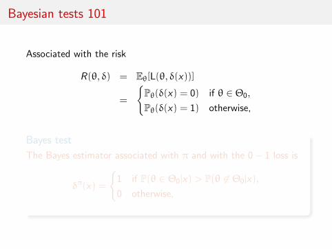
Bayesian tests 101
Associated with the risk
R(θ, δ) = Eθ[L(θ, δ(x))]
=
{Pθ(δ(x) = 0) if θ ∈ Θ0,
Pθ(δ(x) = 1) otherwise,
Bayes test
The Bayes estimator associated with π and with the 0 − 1 loss is
δπ(x) =
{1 if P(θ ∈ Θ0|x) > P(θ 6∈ Θ0|x),
0 otherwise,

Bayesian tests 101
Associated with the risk
R(θ, δ) = Eθ[L(θ, δ(x))]
=
{Pθ(δ(x) = 0) if θ ∈ Θ0,
Pθ(δ(x) = 1) otherwise,
Bayes test
The Bayes estimator associated with π and with the 0 − 1 loss is
δπ(x) =
{1 if P(θ ∈ Θ0|x) > P(θ 6∈ Θ0|x),
0 otherwise,

Bayesian tests 102
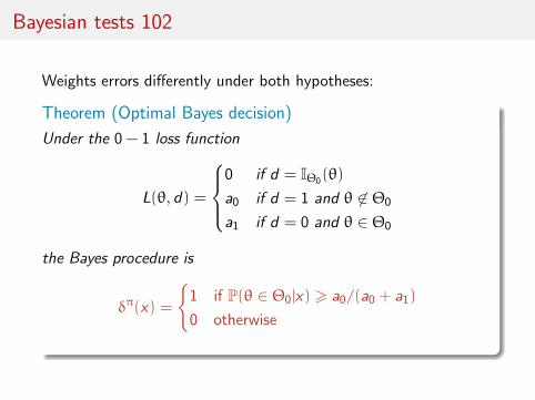
Weights errors differently under both hypotheses:
Theorem (Optimal Bayes decision)
Under the 0 − 1 loss function
L(θ, d) =
0 if d = IΘ0(θ)
a0 if d = 1 and θ 6∈ Θ0
a1 if d = 0 and θ ∈ Θ0
the Bayes procedure is
δπ(x) =
{1 if P(θ ∈ Θ0|x) > a0/(a0 + a1)
0 otherwise
Bayesian tests 102
Weights errors differently under both hypotheses:
Theorem (Optimal Bayes decision)
Under the 0 − 1 loss function
L(θ, d) =
0 if d = IΘ0(θ)
a0 if d = 1 and θ 6∈ Θ0
a1 if d = 0 and θ ∈ Θ0
the Bayes procedure is
δπ(x) =
{1 if P(θ ∈ Θ0|x) > a0/(a0 + a1)
0 otherwise

A function of posterior probabilities
Definition (Bayes factors)
For hypotheses H0 : θ ∈ Θ0 vs. Ha : θ 6∈ Θ0
B01 =π(Θ0|x)
π(Θc0|x)
/π(Θ0)
π(Θc0)
=
∫Θ0
f (x |θ)π0(θ)dθ∫Θc
0
f (x |θ)π1(θ)dθ
[Jeffreys, ToP, 1939, V, §5.01]
Bayes rule under 0 − 1 loss: acceptance if
B01 > {(1 − π(Θ0))/a1}/{π(Θ0)/a0}

self-contained concept
Outside decision-theoretic environment:
I eliminates choice of π(Θ0)
I but depends on the choice of (π0,π1)
I Bayesian/marginal equivalent to the likelihood ratioI Jeffreys’ scale of evidence:
I if log10(Bπ10) between 0 and 0.5, evidence against H0 weak,
I if log10(Bπ10) 0.5 and 1, evidence substantial,
I if log10(Bπ10) 1 and 2, evidence strong and
I if log10(Bπ10) above 2, evidence decisive
[...fairly arbitrary!]

consistency
Example of a normal Xn ∼ N(µ, 1/n) when µ ∼ N(0, 1), leading to
B01 = (1 + n)−1/2 exp{n2x2
n/2(1 + n)}

Some difficulties
I tension between using (i) posterior probabilities justified bybinary loss function but depending on unnatural prior weights,and (ii) Bayes factors that eliminate dependence but escapedirect connection with posterior, unless prior weights areintegrated within loss
I delicate interpretation (or calibration) of strength of the Bayesfactor towards supporting a given hypothesis or model,because not a Bayesian decision rule
I similar difficulty with posterior probabilities, with tendency tointerpret them as p-values: only report of respective strengthsof fitting data to both models

Some difficulties
I tension between using (i) posterior probabilities justified bybinary loss function but depending on unnatural prior weights,and (ii) Bayes factors that eliminate dependence but escapedirect connection with posterior, unless prior weights areintegrated within loss
I referring to a fixed and arbitrary cuttoff value falls into thesame difficulties as regular p-values
I no “third way” like opting out from a decision

Some further difficulties
I long-lasting impact of prior modeling, i.e., choice of priordistributions on parameters of both models, despite overallconsistency proof for Bayes factor
I discontinuity in valid use of improper priors since they are notjustified in most testing situations, leading to many alternativeand ad hoc solutions, where data is either used twice or splitin artificial ways [or further tortured into confession]
I binary (accept vs. reject) outcome more suited for immediatedecision (if any) than for model evaluation, in connection withrudimentary loss function [atavistic remain ofNeyman-Pearson formalism]

Some additional difficulties
I related impossibility to ascertain simultaneous misfit or todetect outliers
I no assessment of uncertainty associated with decision itselfbesides posterior probability
I difficult computation of marginal likelihoods in most settingswith further controversies about which algorithm to adopt
I strong dependence of posterior probabilities on conditioningstatistics (ABC), which undermines their validity for modelassessment
I temptation to create pseudo-frequentist equivalents such asq-values with even less Bayesian justifications
I c© time for a paradigm shift
I back to some solutions

Historical appearance of Bayesian tests
Is the new parameter supported by the observations or isany variation expressible by it better interpreted asrandom? Thus we must set two hypotheses forcomparison, the more complicated having the smallerinitial probability
...compare a specially suggested value of a newparameter, often 0 [q], with the aggregate of otherpossible values [q′]. We shall call q the null hypothesisand q′ the alternative hypothesis [and] we must take
P(q|H) = P(q′|H) = 1/2 .
(Jeffreys, ToP, 1939, V, §5.0)

A major refurbishment
Suppose we are considering whether a location parameterα is 0. The estimation prior probability for it is uniformand we should have to take f (α) = 0 and K [= B10]would always be infinite (Jeffreys, ToP, V, §5.02)
When the null hypothesis is supported by a set of measure 0against Lebesgue measure, π(Θ0) = 0 for an absolutely continuousprior distribution
[End of the story?!]

A major refurbishment
When the null hypothesis is supported by a set of measure 0against Lebesgue measure, π(Θ0) = 0 for an absolutely continuousprior distribution
[End of the story?!]
Requirement
Defined prior distributions under both assumptions,
π0(θ) ∝ π(θ)IΘ0(θ), π1(θ) ∝ π(θ)IΘ1(θ),
(under the standard dominating measures on Θ0 and Θ1)

A major refurbishment
When the null hypothesis is supported by a set of measure 0against Lebesgue measure, π(Θ0) = 0 for an absolutely continuousprior distribution
[End of the story?!]Using the prior probabilities π(Θ0) = ρ0 and π(Θ1) = ρ1,
π(θ) = ρ0π0(θ) + ρ1π1(θ).

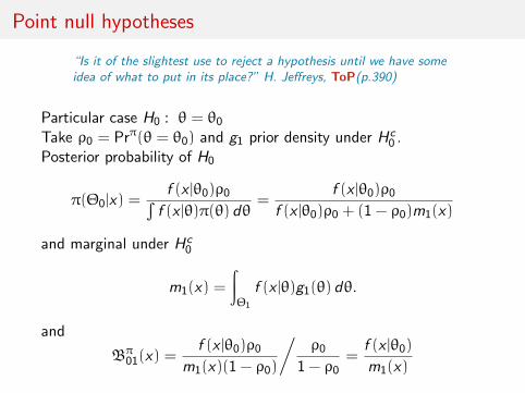
Point null hypotheses
“Is it of the slightest use to reject a hypothesis until we have someidea of what to put in its place?” H. Jeffreys, ToP(p.390)
Particular case H0 : θ = θ0Take ρ0 = Prπ(θ = θ0) and g1 prior density under Hc
0 .Posterior probability of H0
π(Θ0|x) =f (x |θ0)ρ0∫
f (x |θ)π(θ) dθ=
f (x |θ0)ρ0f (x |θ0)ρ0 + (1 − ρ0)m1(x)
and marginal under Hc0
m1(x) =
∫Θ1
f (x |θ)g1(θ) dθ.
and
Bπ01(x) =
f (x |θ0)ρ0m1(x)(1 − ρ0)
/ρ0
1 − ρ0=
f (x |θ0)
m1(x)

Noninformative proposals
Bayesian testing of hypotheses
Noninformative solutions
Testing via mixtures
Paradigm shift

what’s special about the Bayes factor?!
I “The priors do not represent substantive knowledge of theparameters within the model
I Using Bayes’ theorem, these priors can then be updated toposteriors conditioned on the data that were actually observed
I In general, the fact that different priors result in differentBayes factors should not come as a surprise
I The Bayes factor (...) balances the tension between parsimonyand goodness of fit, (...) against overfitting the data
I In induction there is no harm in being occasionally wrong; it isinevitable that we shall be”
[Jeffreys, 1939; Ly et al., 2015]

what’s wrong with the Bayes factor?!
I (1/2, 1/2) partition between hypotheses has very little tosuggest in terms of extensions
I central difficulty stands with issue of picking a priorprobability of a model
I unfortunate impossibility of using improper priors in mostsettings
I Bayes factors lack direct scaling associated with posteriorprobability and loss function
I twofold dependence on subjective prior measure, first in priorweights of models and second in lasting impact of priormodelling on the parameters
I Bayes factor offers no window into uncertainty associated withdecision
I further reasons in the summary
[Robert, 2016]

Lindley’s paradox
In a normal mean testing problem,
xn ∼ N(θ,σ2/n) , H0 : θ = θ0 ,
under Jeffreys prior, θ ∼ N(θ0,σ2), the Bayes factor
B01(tn) = (1 + n)1/2 exp(−nt2n/2[1 + n]
),
where tn =√
n|xn − θ0|/σ, satisfies
B01(tn)n−→∞−→ ∞
[assuming a fixed tn][Lindley, 1957]
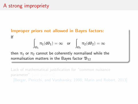
A strong impropriety
Improper priors not allowed in Bayes factors:
If ∫Θ1
π1(dθ1) =∞ or
∫Θ2
π2(dθ2) =∞then π1 or π2 cannot be coherently normalised while thenormalisation matters in the Bayes factor B12
Lack of mathematical justification for “common nuisanceparameter” [and prior of]
[Berger, Pericchi, and Varshavsky, 1998; Marin and Robert, 2013]
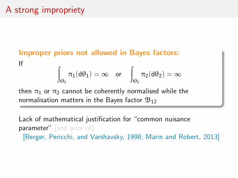

On some resolutions of the paradox
I use of pseudo-Bayes factors, fractional Bayes factors, &tc,which lacks complete proper Bayesian justification
[Berger & Pericchi, 2001]
I use of identical improper priors on nuisance parameters,
I calibration via the posterior predictive distribution,
I matching priors,
I use of score functions extending the log score function
I non-local priors correcting default priors

On some resolutions of the paradox
I use of pseudo-Bayes factors, fractional Bayes factors, &tc,
I use of identical improper priors on nuisance parameters, anotion already entertained by Jeffreys
[Berger et al., 1998; Marin & Robert, 2013]
I calibration via the posterior predictive distribution,
I matching priors,
I use of score functions extending the log score function
I non-local priors correcting default priors

On some resolutions of the paradox
I use of pseudo-Bayes factors, fractional Bayes factors, &tc,
I use of identical improper priors on nuisance parameters,
I Peche de jeunesse: equating the values of the prior densitiesat the point-null value θ0,
ρ0 = (1 − ρ0)π1(θ0)
[Robert, 1993]
I calibration via the posterior predictive distribution,
I matching priors,
I use of score functions extending the log score function
I non-local priors correcting default priors

On some resolutions of the paradox
I use of pseudo-Bayes factors, fractional Bayes factors, &tc,
I use of identical improper priors on nuisance parameters,
I calibration via the posterior predictive distribution, which usesthe data twice
I matching priors,
I use of score functions extending the log score function
I non-local priors correcting default priors

On some resolutions of the paradox
I use of pseudo-Bayes factors, fractional Bayes factors, &tc,
I use of identical improper priors on nuisance parameters,
I calibration via the posterior predictive distribution,
I matching priors, whose sole purpose is to bring frequentistand Bayesian coverages as close as possible
[Datta & Mukerjee, 2004]
I use of score functions extending the log score function
I non-local priors correcting default priors

On some resolutions of the paradox
I use of pseudo-Bayes factors, fractional Bayes factors, &tc,
I use of identical improper priors on nuisance parameters,
I calibration via the posterior predictive distribution,
I matching priors,
I use of score functions extending the log score function
logB12(x) = log m1(x) − log m2(x) = S0(x , m1) − S0(x , m2) ,
that are independent of the normalising constant[Dawid et al., 2013; Dawid & Musio, 2015]
I non-local priors correcting default priors

On some resolutions of the paradox
I use of pseudo-Bayes factors, fractional Bayes factors, &tc,
I use of identical improper priors on nuisance parameters,
I calibration via the posterior predictive distribution,
I matching priors,
I use of score functions extending the log score function
I non-local priors correcting default priors towards morebalanced error rates
[Johnson & Rossell, 2010; Consonni et al., 2013]

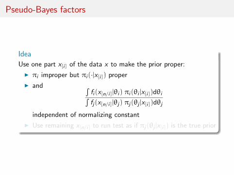
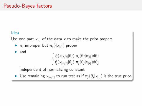
Pseudo-Bayes factors
Idea
Use one part x[i] of the data x to make the prior proper:
I πi improper but πi (·|x[i]) proper
I and ∫fi (x[n/i]|θi ) πi (θi |x[i])dθi∫fj(x[n/i]|θj) πj(θj |x[i])dθj
independent of normalizing constant
I Use remaining x[n/i] to run test as if πj(θj |x[i]) is the true prior
Pseudo-Bayes factors
Idea
Use one part x[i] of the data x to make the prior proper:
I πi improper but πi (·|x[i]) proper
I and ∫fi (x[n/i]|θi ) πi (θi |x[i])dθi∫fj(x[n/i]|θj) πj(θj |x[i])dθj
independent of normalizing constant
I Use remaining x[n/i] to run test as if πj(θj |x[i]) is the true prior
Pseudo-Bayes factors
Idea
Use one part x[i] of the data x to make the prior proper:
I πi improper but πi (·|x[i]) proper
I and ∫fi (x[n/i]|θi ) πi (θi |x[i])dθi∫fj(x[n/i]|θj) πj(θj |x[i])dθj
independent of normalizing constant
I Use remaining x[n/i] to run test as if πj(θj |x[i]) is the true prior

Motivation
I Provides a working principle for improper priors
I Gather enough information from data to achieve properness
I and use this properness to run the test on remaining data
I does not use x twice as in Aitkin’s (1991)

Motivation
I Provides a working principle for improper priors
I Gather enough information from data to achieve properness
I and use this properness to run the test on remaining data
I does not use x twice as in Aitkin’s (1991)

Motivation
I Provides a working principle for improper priors
I Gather enough information from data to achieve properness
I and use this properness to run the test on remaining data
I does not use x twice as in Aitkin’s (1991)

Issues
I depends on the choice of x[i]I many ways of combining pseudo-Bayes factors
I AIBF = BNji
1
L
∑`
Bij(x[`])
I MIBF = BNji med[Bij(x[`])]
I GIBF = BNji exp
1
L
∑`
log Bij(x[`])
I not often an exact Bayes factor
I and thus lacking inner coherence
B12 6= B10B02 and B01 6= 1/B10 .
[Berger & Pericchi, 1996]

Fractional Bayes factor
Idea
use directly the likelihood to separate training sample from testingsample
BF12 = B12(x)
∫Lb2(θ2)π2(θ2)dθ2∫
Lb1(θ1)π1(θ1)dθ1
[O’Hagan, 1995]
Proportion b of the sample used to gain proper-ness

Fractional Bayes factor
Idea
use directly the likelihood to separate training sample from testingsample
BF12 = B12(x)
∫Lb2(θ2)π2(θ2)dθ2∫
Lb1(θ1)π1(θ1)dθ1
[O’Hagan, 1995]
Proportion b of the sample used to gain proper-ness

Fractional Bayes factor (cont’d)
Example (Normal mean)
BF12 =
1√b
en(b−1)x2n/2
corresponds to exact Bayes factor for the prior N(0, 1−b
nb
)I If b constant, prior variance goes to 0
I If b =1
n, prior variance stabilises around 1
I If b = n−α, α < 1, prior variance goes to 0 too.
c© Call to external principles to pick the order of b
Bayesian predictive
“If the model fits, then replicated data generated underthe model should look similar to observed data. To put itanother way, the observed data should look plausibleunder the posterior predictive distribution. This is really aself-consistency check: an observed discrepancy can bedue to model misfit or chance.” (BDA, p.143)
Use of posterior predictive
p(y rep|y) =
∫p(y rep|θ)π(θ|y) dθ
and measure of discrepancy T (·, ·)Replacing p-value
p(y |θ) = P(T (y rep, θ) > T (y , θ)|θ)
with Bayesian posterior p-value
P(T (y rep, θ) > T (y , θ)|y) =
∫p(y |θ)π(θ|x) dθ

Issues
“the posterior predictive p-value is such a [Bayesian]probability statement, conditional on the model and data,about what might be expected in future replications.(BDA, p.151)
I sounds too much like a p-value...!
I relies on choice of T (·, ·)I seems to favour overfitting
I (again) using the data twice (once for the posterior and twicein the p-value)
I needs to be calibrated (back to 0.05?)
I general difficulty in interpreting
I where is the penalty for model complexity?
Changing the testing perspective
Bayesian testing of hypotheses
Noninformative solutions
Testing via mixtures
Paradigm shift

Paradigm shift
New proposal for a paradigm shift (!) in the Bayesian processing ofhypothesis testing and of model selection
I convergent and naturally interpretable solution
I more extended use of improper priors
Simple representation of the testing problem as atwo-component mixture estimation problem where theweights are formally equal to 0 or 1

Paradigm shift
Simple representation of the testing problem as atwo-component mixture estimation problem where theweights are formally equal to 0 or 1
I Approach inspired from consistency result of Rousseau andMengersen (2011) on estimated overfitting mixtures
I Mixture representation not directly equivalent to the use of aposterior probability
I Potential of a better approach to testing, while not expandingnumber of parameters
I Calibration of posterior distribution of the weight of a model,moving from artificial notion of posterior probability of amodel
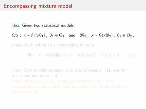
Encompassing mixture model
Idea: Given two statistical models,
M1 : x ∼ f1(x |θ1) , θ1 ∈ Θ1 and M2 : x ∼ f2(x |θ2) , θ2 ∈ Θ2 ,
embed both within an encompassing mixture
Mα : x ∼ αf1(x |θ1) + (1 − α)f2(x |θ2) , 0 6 α 6 1 (1)
Note: Both models correspond to special cases of (1), one forα = 1 and one for α = 0Draw inference on mixture representation (1), as if eachobservation was individually and independently produced by themixture model

Inferential motivations
Sounds like approximation to the real model, but several definitiveadvantages to this paradigm shift:
I Bayes estimate of the weight α replaces posterior probabilityof model M1, equally convergent indicator of which model is“true”, while avoiding artificial prior probabilities on modelindices, ω1 and ω2
I interpretation of estimator of α at least as natural as handlingthe posterior probability, while avoiding zero-one loss setting
I α and its posterior distribution provide measure of proximityto the models, while being interpretable as data propensity tostand within one model
I further allows for alternative perspectives on testing andmodel choice, like predictive tools, cross-validation, andinformation indices like WAIC

Computational motivations
I avoids highly problematic computations of the marginallikelihoods, since standard algorithms are available forBayesian mixture estimation
I straightforward extension to a finite collection of models, witha larger number of components, which considers all models atonce and eliminates least likely models by simulation
I eliminates difficulty of label switching that plagues bothBayesian estimation and Bayesian computation, sincecomponents are no longer exchangeable
I posterior distribution of α evaluates more thoroughly strengthof support for a given model than the single figure outcome ofa posterior probability
I variability of posterior distribution on α allows for a morethorough assessment of the strength of this support

Noninformative motivations
I additional feature missing from traditional Bayesian answers:a mixture model acknowledges possibility that, for a finitedataset, both models or none could be acceptable
I standard (proper and informative) prior modeling can bereproduced in this setting, but non-informative (improper)priors also are manageable therein, provided both models firstreparameterised towards shared parameters, e.g. location andscale parameters
I in special case when all parameters are common
Mα : x ∼ αf1(x |θ) + (1 − α)f2(x |θ) , 0 6 α 6 1
if θ is a location parameter, a flat prior π(θ) ∝ 1 is available
Weakly informative motivations
I using the same parameters or some identical parameters onboth components highlights that opposition between the twocomponents is not an issue of enjoying different parameters
I those common parameters are nuisance parameters, to beintegrated out [unlike Lindley’s paradox]
I prior model weights ωi rarely discussed in classical Bayesianapproach, even though linear impact on posterior probabilities.Here, prior modeling only involves selecting a prior on α, e.g.,α ∼ B(a0, a0)
I while a0 impacts posterior on α, it always leads to massaccumulation near 1 or 0, i.e. favours most likely model
I sensitivity analysis straightforward to carry
I approach easily calibrated by parametric boostrap providingreference posterior of α under each model
I natural Metropolis–Hastings alternative
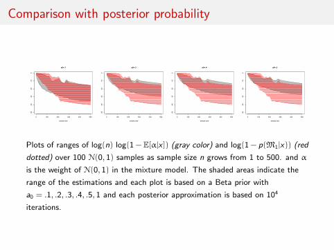
Comparison with posterior probability
0 100 200 300 400 500
-50
-40
-30
-20
-10
0
a0=.1
sample size
0 100 200 300 400 500
-50
-40
-30
-20
-10
0
a0=.3
sample size
0 100 200 300 400 500
-50
-40
-30
-20
-10
0
a0=.4
sample size
0 100 200 300 400 500
-50
-40
-30
-20
-10
0
a0=.5
sample size
Plots of ranges of log(n) log(1−E[α|x ]) (gray color) and log(1− p(M1|x)) (red
dotted) over 100 N(0, 1) samples as sample size n grows from 1 to 500. and α
is the weight of N(0, 1) in the mixture model. The shaded areas indicate the
range of the estimations and each plot is based on a Beta prior with
a0 = .1, .2, .3, .4, .5, 1 and each posterior approximation is based on 104
iterations.

Towards which decision?
And if we have to make a decision?
soft consider behaviour of posterior under prior predictives
I or posterior predictive [e.g., prior predictive does not exist]
I boostrapping behaviour
I comparison with Bayesian non-parametric solution
hard rethink the loss function

Conclusion
I many applications of the Bayesian paradigm concentrate onthe comparison of scientific theories and on testing of nullhypotheses
I natural tendency to default to Bayes factors
I poorly understood sensitivity to prior modeling and posteriorcalibration
c© Time is ripe for a paradigm shift

Down with Bayes factors!
c© Time is ripe for a paradigm shift
I original testing problem replaced with a better controlledestimation target
I allow for posterior variability over the component frequency asopposed to deterministic Bayes factors
I range of acceptance, rejection and indecision conclusionseasily calibrated by simulation
I posterior medians quickly settling near the boundary values of0 and 1
I potential derivation of a Bayesian b-value by looking at theposterior area under the tail of the distribution of the weight

Prior modelling
c© Time is ripe for a paradigm shift
I Partly common parameterisation always feasible and henceallows for reference priors
I removal of the absolute prohibition of improper priors inhypothesis testing
I prior on the weight α shows sensitivity that naturally vanishesas the sample size increases
I default value of a0 = 0.5 in the Beta prior

Computing aspects
c© Time is ripe for a paradigm shift
I proposal that does not induce additional computational strain
I when algorithmic solutions exist for both models, they can berecycled towards estimating the encompassing mixture
I easier than in standard mixture problems due to commonparameters that allow for original MCMC samplers to beturned into proposals
I Gibbs sampling completions useful for assessing potentialoutliers but not essential to achieve a conclusion about theoverall problem