bayesian networks and their applications in systems biology · bayesian networks and their...

Bayesian networks and their applications in systems biology

Marco Grzegorczyk

41st Statistical Computing Workshop

Schloss Reisensburg, Günzburg 30-Jun-09

Outline 1. Introduction

2. Static Bayesian networks

3. Dynamic Bayesian networks

4. Non-stationary gene regulatory processes

4.1 BGM

4.2 BGMD

4.3 BGMD,2

Cell Biology

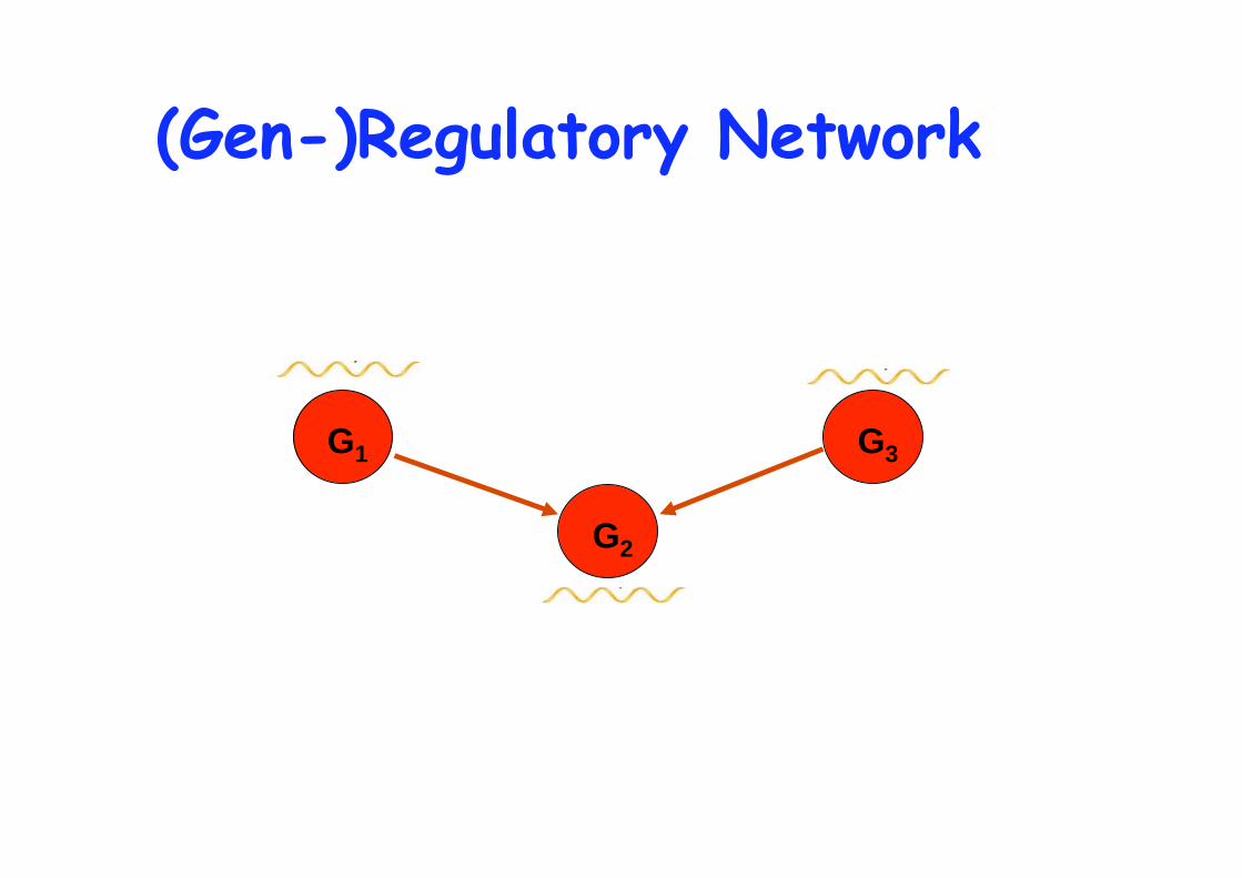
(Gen-)Regulatory Network

TF TF

metabolite A metabolite B

G2 G3 G1

P1 P3 P2

G1

mRNA(G1) mRNA(G3) mRNA(G2)

Protein P1 is transcription factor for gene G2

Protein P3 is transcription

factor for gene G2 Protein P2 is an enzym catalysing a metabolic

reaction

Microarray Chips

Expressions (activities) of thousands of genes in an experimental cell can be measured with Microarray Chips.

TF TF

metabolite A metabolite B

G2 G3 G1

P1 P3 P2

G1


G2

G3 G1 G1


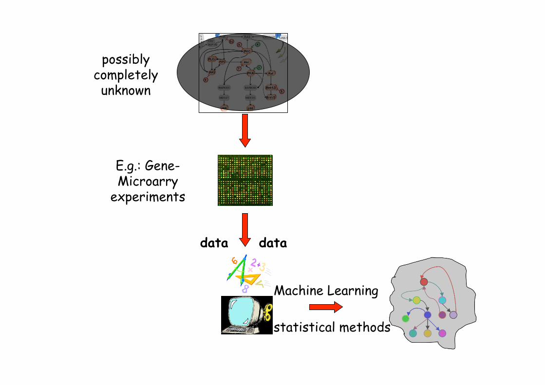
possibly completely unknown


E.g.: Gene-Microarry

experiments data

(expressions of genes)


data data

Machine Learning

statistical methods

E.g.: Gene-Microarry

experiments

Statistical Task

cells

variables

X1,...Xn

(genes)

Extract a network from a data matrix

m independent (steady-state) observations

of the system X1,…,XN





4.1 BGM

4.2 BGMD

4.3 BGMD,2

Static Bayesian networks

A

C B

D

E F

NODES

EDGES

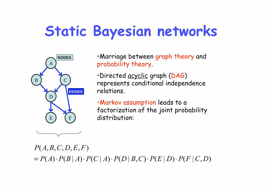
•Marriage between graph theory and probability theory.

•Directed acyclic graph (DAG) represents conditional independence relations.

•Markov assumption leads to a factorization of the joint probability distribution:


A

C B

D

E F

NODES

EDGES

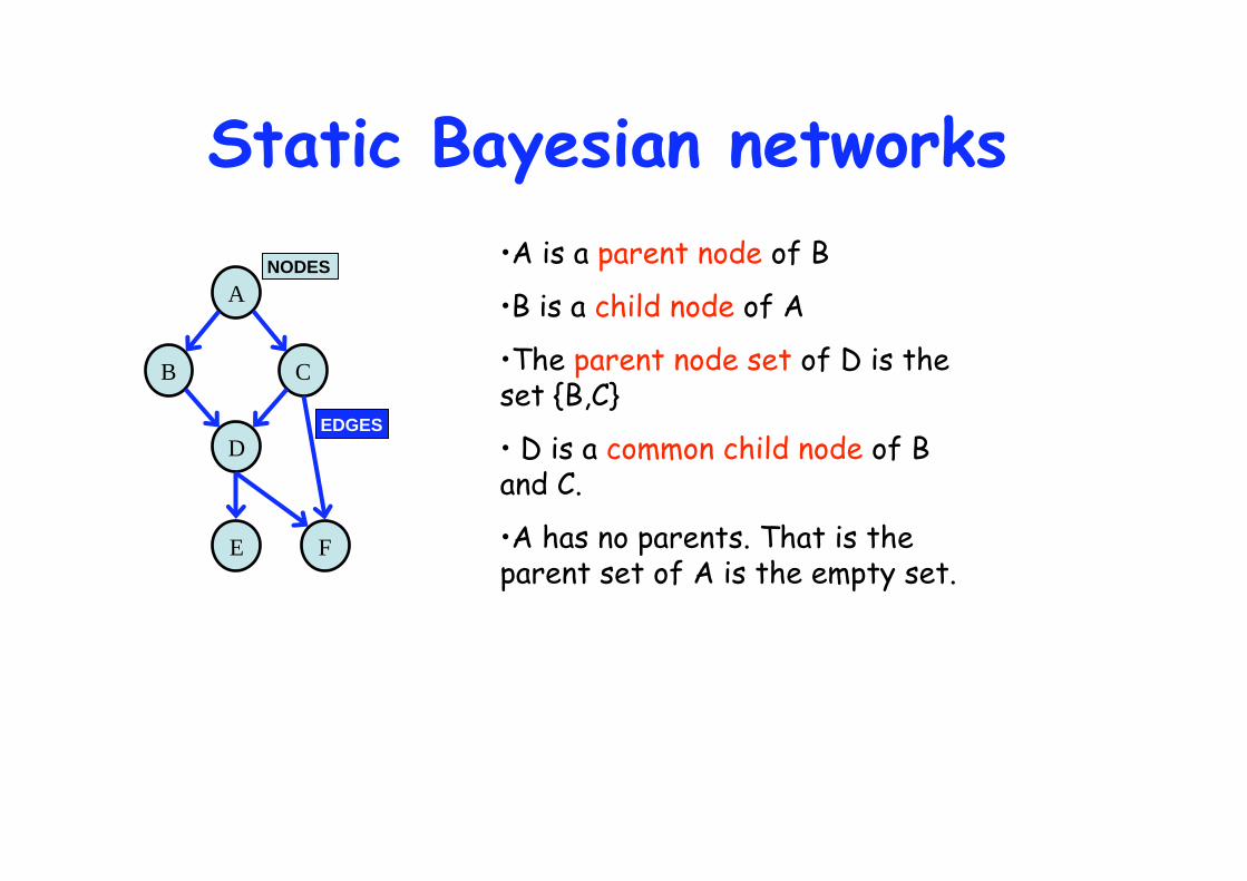
•A is a parent node of B

•B is a child node of A

•The parent node set of D is the set {B,C}

• D is a common child node of B and C.

•A has no parents. That is the parent set of A is the empty set.


A

C B

D

E F

NODES

EDGES

•A has no ancestor nodes (ancestors)

•B has one ancestor node: A

•C has one ancestor node: A

•D has three ancestor nodes A,B, and C

•E and F have four ancestor nodes each: A,B,C, and D

Equivalence classes of BNs A

B

C

A

B

A

B

A

B

C

C

C

A

B

C

completed partially

directed graphs

(CPDAGs)

A

C

B

v-structure P(A,B)=P(A)·P(B)

P(A,B|C) P(A|C)·P(B|C)

P(A,B) P(A)·P(B)

P(A,B|C)=P(A|C)·P(B|C)

Sytematic Overview – Equivalence classes 3 node networks

DAG and its CPDAG

A

C B

D

E F

NODES

EDGES

CPDAG of the DAG on the left Directed Acyclic Graph

(DAG)

A

C B

D

E F

NODES

EDGES

CPDAGs (completed partially directed acyclic graphs)

possess both direct and undirected edges.

Bayesian networks versus causal networks

Bayesian networks represent conditional (in)dependency relations - not necessarily causal interactions.

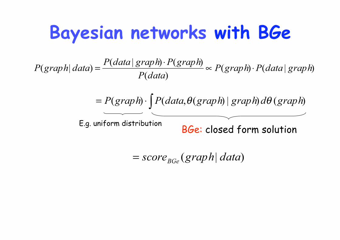
Bayesian networks with BGe


Parameterisation: Gaussian BGe scoring metric:

data~N(μ, )

with normal-Wishart distribution of the (unknown) parameters, i.e.:

μ~N(μ*,(vW)-1) and W= -1 with W~Wishart(T0)


E.g. uniform distribution BGe: closed form solution

Learning the network structure

n 4 6 8 10

#DAGs 543 3,7 106 7,8 1011 4,2 1018

Idea: Heuristically searching for the graph M*

that is most supported by the data

P(M*|data)>P(graph|data),

e.g.: greedy search algorithm

graph score(graph)

Learning the network structure

Distribution of P(graph|data)

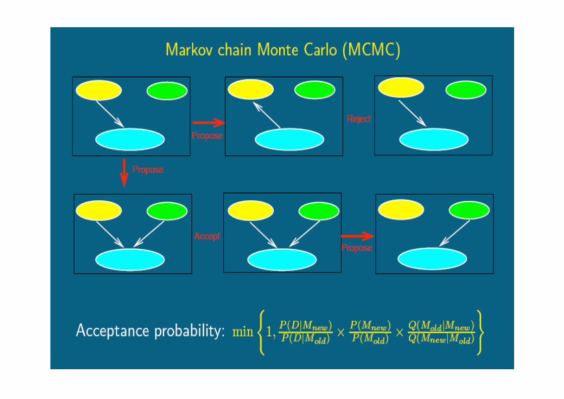
MCMC sampling of Bayesian networks

Better idea: Bayesian model averaging via Markov Chain

Monte Carlo (MCMC) simulations

Construct and simulate a Markov Chain (Mt)t in the space

of DAGs whose distribution converges to the graph

Posterior distribution as stationary distribution, i.e.:

P(Mt=graph|data) P(graph|data)

t

to generate a DAG sample: G1,G2,G3,…GT

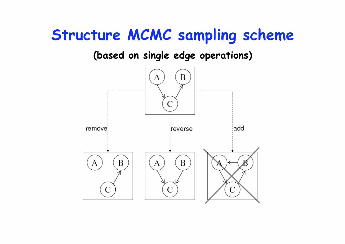
Structure MCMC sampling scheme (based on single edge operations)

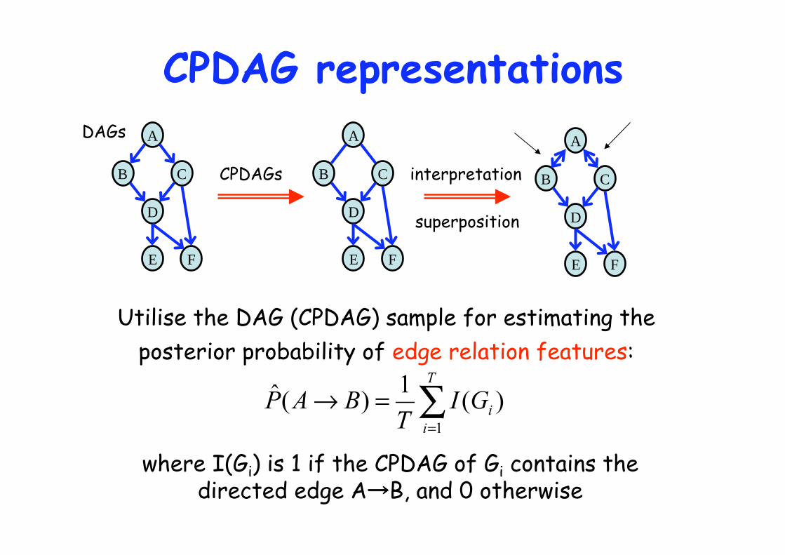
CPDAG representations

A

B C

D

E F

A

B C

D

E F

DAGs

CPDAGs

Utilise the DAG (CPDAG) sample for estimating the

posterior probability of edge relation features:

where I(Gi) is 1 if the CPDAG of Gi contains the directed edge A B, and 0 otherwise

A

B C

D

E F

interpretation

superposition





4.1 BGM

4.2 BGMD

4.3 BGMD,2

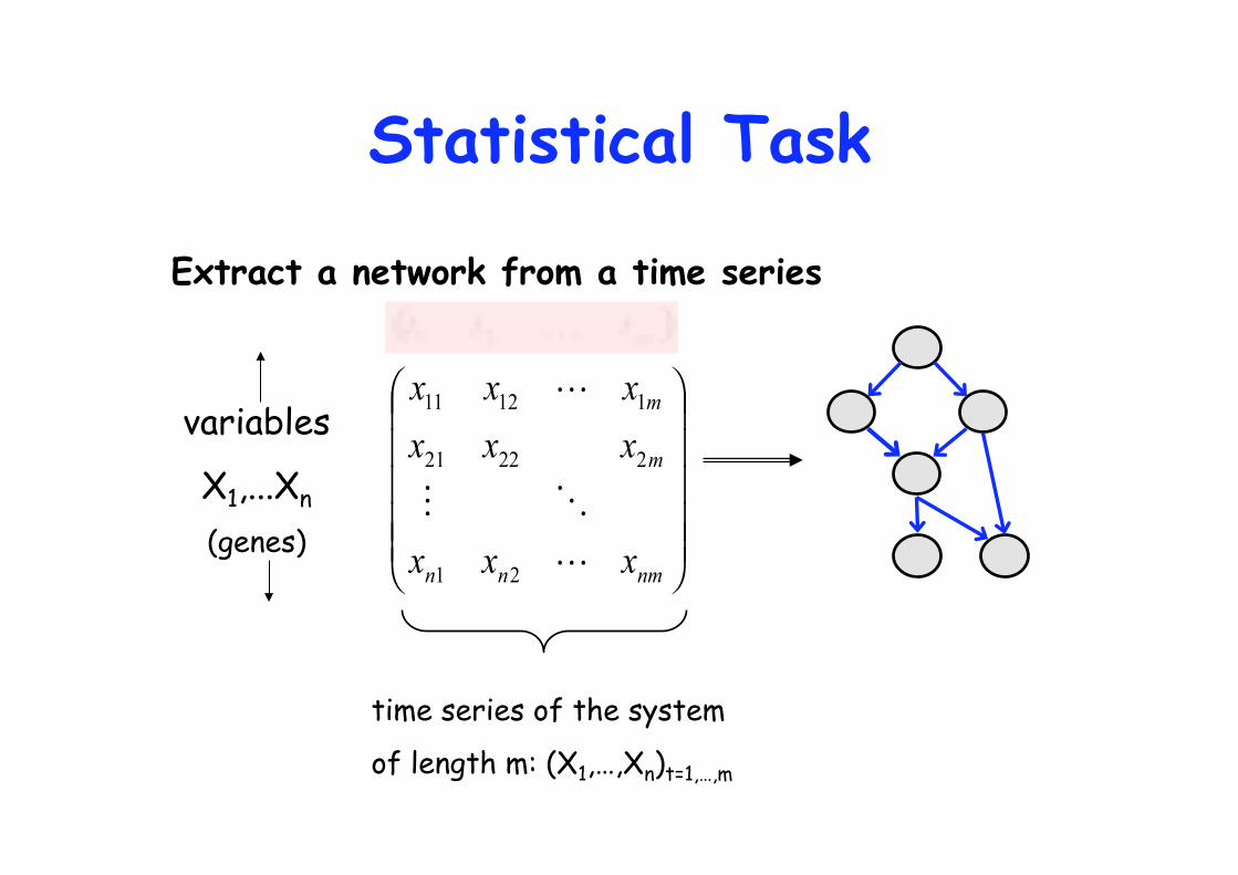
Statistical Task

variables

X1,...Xn

(genes)

Extract a network from a time series

time series of the system

of length m: (X1,…,Xn)t=1,…,m

Dynamic Bayesian networks

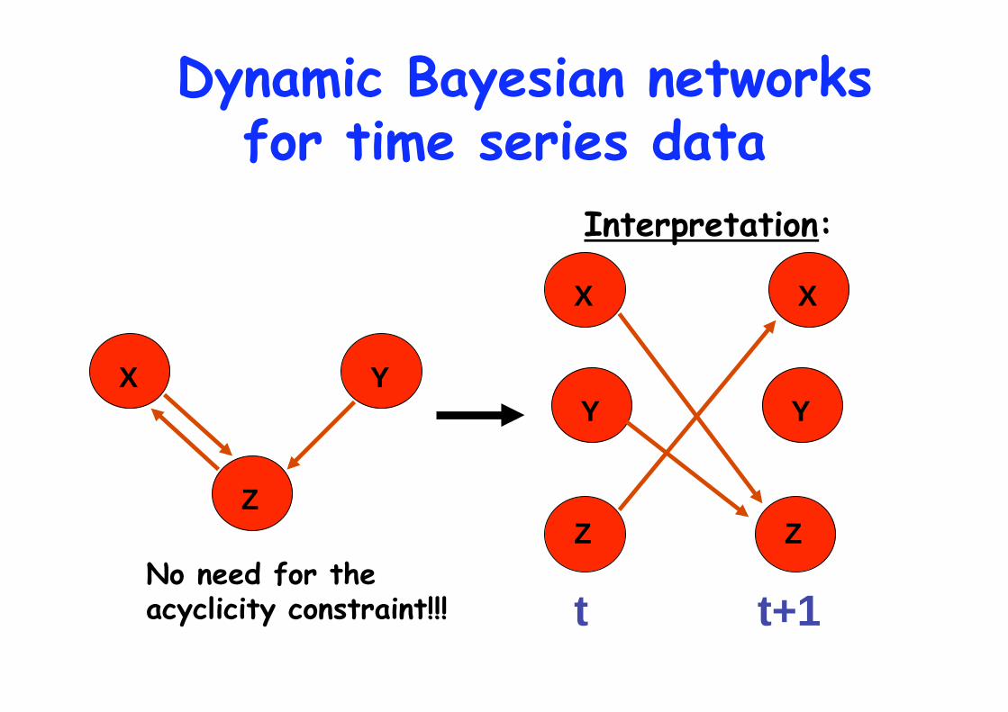
Y

Z

X

Dynamic Bayesian networks for time series data

X X

Y Y

Z Z

t t+1

Interpretation:

No need for the acyclicity constraint!!!

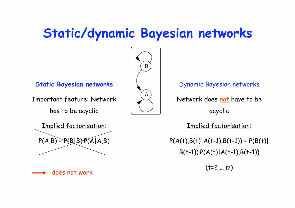
Static/dynamic Bayesian networks


Important feature: Network

has to be acyclic

Implied factorisation:

P(A,B) = P(B|B)·P(A|A,B)

Dynamic Bayesian networks

Network does not have to be

acyclic

Implied factorisation:

P(A(t),B(t)|A(t-1),B(t-1)) = P(B(t)|

B(t-1))·P(A(t)|A(t-1),B(t-1))

(t=2,…,m) does not work

MCMC sampling of Bayesian networks

Better idea: Bayesian model averaging via Markov Chain

Monte Carlo (MCMC) simulations

Construct and simulate a Markov Chain (Mt)t in the space

of DAGs whose distribution converges to the graph

Posterior distribution as stationary distribution, i.e.:

P(Mt=graph|data) P(graph|data)

t

to generate a DAG sample: G1,G2,G3,…GT

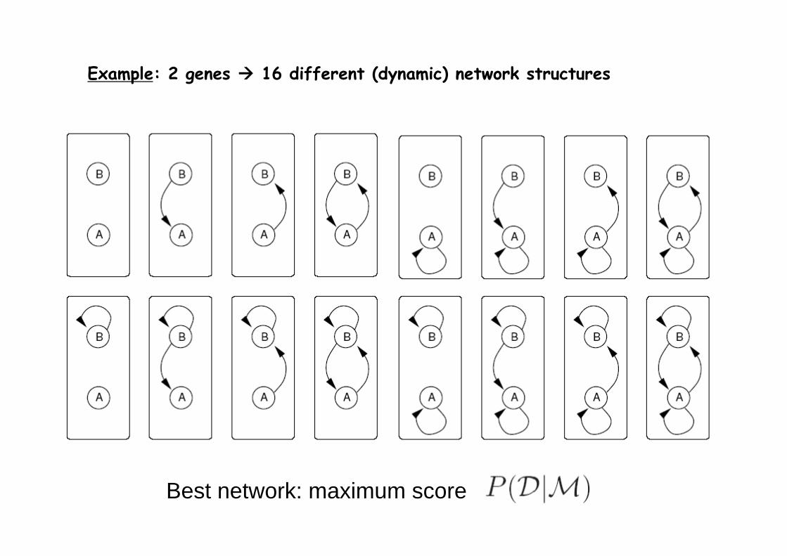
Example: 2 genes 16 different (dynamic) network structures

Best network: maximum score

Identify the best network structure

Ideal scenario: Large data sets, low noise

P(graph|data)

M*

Uncertainty about the best network structure

Limited number of experimental replications, high noise

P(graph|data)

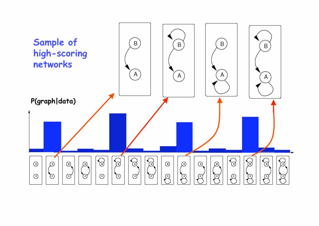
Sample of high-scoring networks

P(graph|data)

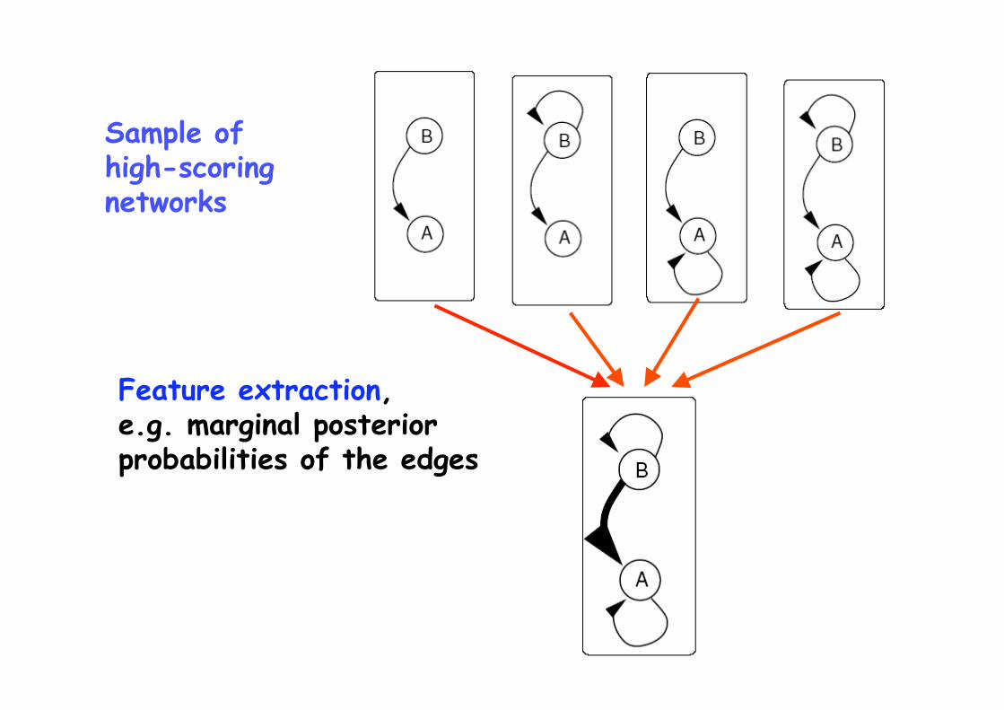
Feature extraction, e.g. marginal posterior probabilities of the edges


Feature extraction, e.g. marginal posterior probabilities of the edges

High-confident edge

High-confident non-edge

Uncertainty about edges


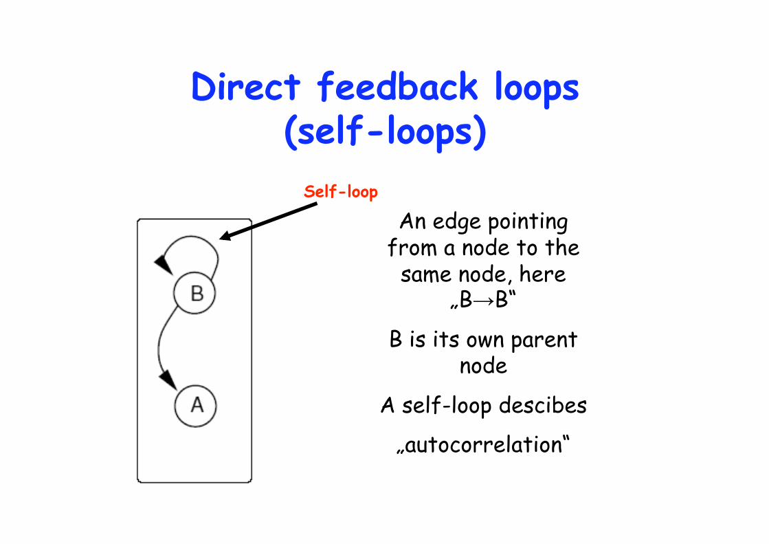
Direct feedback loops (self-loops)

An edge pointing from a node to the

same node, here „B B“

B is its own parent node

A self-loop descibes

„autocorrelation“

Self-loop

Example: 2 genes 16 different (dynamic) network structures

Graphs with self-loops may be considered as invalid





4.1 BGM

4.2 BGMD

4.3 BGMD,2

true network extracted network

Is the extracted network a good prediction of the real relationships?

Reconstruction Accuracy

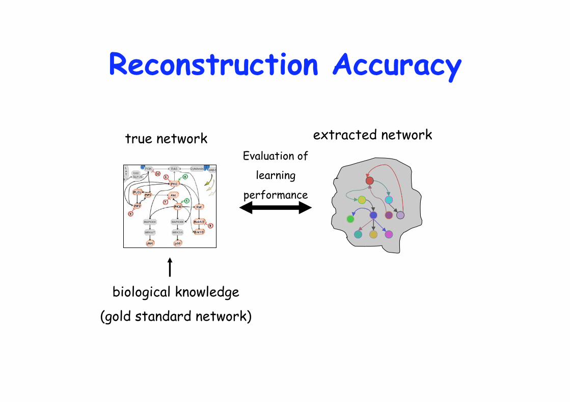
true network extracted network

biological knowledge

(gold standard network)

Evaluation of

learning

performance

Reconstruction Accuracy

data

Probabilistic inference

true regulatory network

Thresholding

edge posterior probabilities

TP:1/2

FP:0/4

TP:2/2

FP:1/4

concrete network predictions

low high

From Perry Sprawls

Evaluation of Performance

AUC scores Area under Receiver Operator Characteristic

(ROC) curve

AUC=0.5 AUC=1 0.5<AUC 1

sens

itiv

ity

inverse specificity





4.1 BGM

4.2 BGMD

4.3 BGMD,2

Modelling non-stationary gene regulatory processes

Standard Bayesian network approaches assume that the process is homogeneous…but processes may be of a heterogeneous nature!

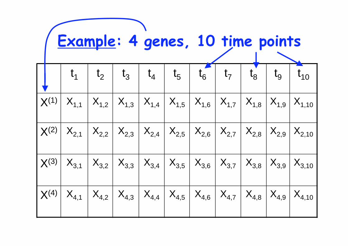
Example: 4 genes, 10 time points

t1 t2 t3 t4 t5 t6 t7 t8 t9 t10

X(1) X1,1 X1,2 X1,3 X1,4 X1,5 X1,6 X1,7 X1,8 X1,9 X1,10

X(2) X2,1 X2,2 X2,3 X2,4 X2,5 X2,6 X2,7 X2,8 X2,9 X2,10

X(3) X3,1 X3,2 X3,3 X3,4 X3,5 X3,6 X3,7 X3,8 X3,9 X3,10

X(4) X4,1 X4,2 X4,3 X4,4 X4,5 X4,6 X4,7 X4,8 X4,9 X4,10

t1 t2 t3 t4 t5 t6 t7 t8 t9 t10

X(1) X1,1 X1,2 X1,3 X1,4 X1,5 X1,6 X1,7 X1,8 X1,9 X1,10

X(2) X2,1 X2,2 X2,3 X2,4 X2,5 X2,6 X2,7 X2,8 X2,9 X2,10

X(3) X3,1 X3,2 X3,3 X3,4 X3,5 X3,6 X3,7 X3,8 X3,9 X3,10

X(4) X4,1 X4,2 X4,3 X4,4 X4,5 X4,6 X4,7 X4,8 X4,9 X4,10

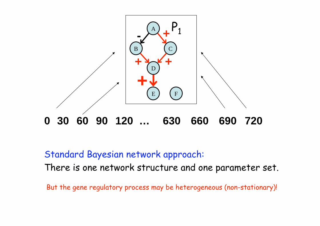
Standard dynamic Bayesian network: homogeneous model

A

C B

D

E F

P1

+

+ -

+ +

630 30 60 120 720 690 660 0 90 …

Standard Bayesian network approach:

There is one network structure and one parameter set.

But the gene regulatory process may be heterogeneous (non-stationary)!

P2 A

C B

D

E F

P1

+

+ -

+ +

A

C B

D

E F

+ -

-

- -

360

630

510

450

420 390

270

600 210

330

480

180

150

30

570

60

300

120

540

240

720

690

660

0

Non-homogeneous process with 2 components

P2

P1

B

P3

A

C B

D

E F

+

+ -

+ +

A

C B

D

E F

-

+

+ -

-

A

C

D

E F

+ -

-

- -

360

630

510

450

420 390

270

600 210

330

480

180

150

30

570

60

300

120

540

240

720

690

0

Non-homogeneous process with 3 components





4.1 BGM

4.2 BGMD

4.3 BGMD,2

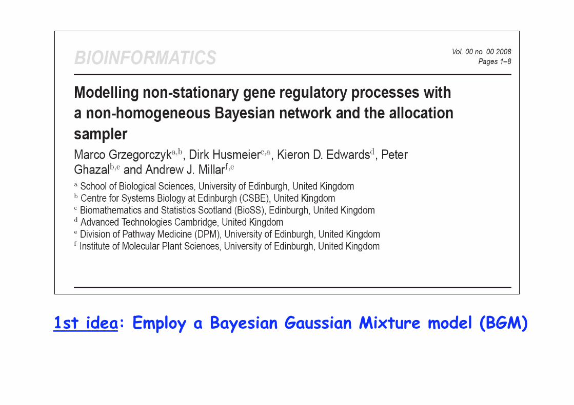
1st idea: Employ a Bayesian Gaussian Mixture model (BGM)

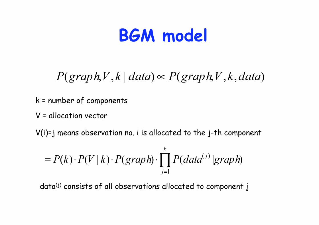
BGM model

k = number of components

V = allocation vector V(i)=j means observation no. i is allocated to the j-th component

data(j) consists of all observations allocated to component j



Poisson Binomial Uniform BGe score

for each subset of data

BGM model



MCMC output:

BGM inference (MCMC)

Example: 4 genes, 10 time points

t1 t2 t3 t4 t5 t6 t7 t8 t9 t10

X(1) X1,1 X1,2 X1,3 X1,4 X1,5 X1,6 X1,7 X1,8 X1,9 X1,10

X(2) X2,1 X2,2 X2,3 X2,4 X2,5 X2,6 X2,7 X2,8 X2,9 X2,10

X(3) X3,1 X3,2 X3,3 X3,4 X3,5 X3,6 X3,7 X3,8 X3,9 X3,10

X(4) X4,1 X4,2 X4,3 X4,4 X4,5 X4,6 X4,7 X4,8 X4,9 X4,10

t1 t2 t3 t4 t5 t6 t7 t8 t9 t10

X(1) X1,1 X1,2 X1,3 X1,4 X1,5 X1,6 X1,7 X1,8 X1,9 X1,10

X(2) X2,1 X2,2 X2,3 X2,4 X2,5 X2,6 X2,7 X2,8 X2,9 X2,10

X(3) X3,1 X3,2 X3,3 X3,4 X3,5 X3,6 X3,7 X3,8 X3,9 X3,10

X(4) X4,1 X4,2 X4,3 X4,4 X4,5 X4,6 X4,7 X4,8 X4,9 X4,10

Standard dynamic Bayesian network: homogeneous model (‘one block’)

BGM model: heterogeneous dynamic Bayesian network. Here: 2 components

t1 t2 t3 t4 t5 t6 t7 t8 t9 t10

X(1) X1,1 X1,2 X1,3 X1,4 X1,5 X1,6 X1,7 X1,8 X1,9 X1,10

X(2) X2,1 X2,2 X2,3 X2,4 X2,5 X2,6 X2,7 X2,8 X2,9 X2,10

X(3) X3,1 X3,2 X3,3 X3,4 X3,5 X3,6 X3,7 X3,8 X3,9 X3,10

X(4) X4,1 X4,2 X4,3 X4,4 X4,5 X4,6 X4,7 X4,8 X4,9 X4,10

t1 t2 t3 t4 t5 t6 t7 t8 t9 t10

X(1) X1,1 X1,2 X1,3 X1,4 X1,5 X1,6 X1,7 X1,8 X1,9 X1,10

X(2) X2,1 X2,2 X2,3 X2,4 X2,5 X2,6 X2,7 X2,8 X2,9 X2,10

X(3) X3,1 X3,2 X3,3 X3,4 X3,5 X3,6 X3,7 X3,8 X3,9 X3,10

X(4) X4,1 X4,2 X4,3 X4,4 X4,5 X4,6 X4,7 X4,8 X4,9 X4,10

BGM model: heterogeneous dynamic Bayesian network. Here: 3 components

Inference with BGM model

q

k

h

Number of components (here: 3)

allocation vector

1. BGM inference:

synthetic pathway data

Raf-Mek-Erk Pathway

Generate

synthetic static Gaussian data

from well-studied

Raf-Mek-Erk pathway

For each number of mixture

components KTRUE (KTRUE=1,…,5)

generate 5 synthetic data sets

consisting of 480 data points

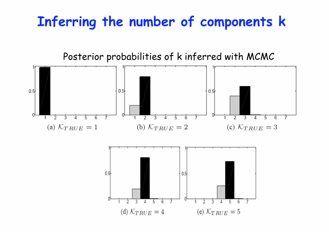
Inferring the number of components k

Posterior probabilities of k inferred with MCMC

Global network reconstruction accuracy in terms auf AUC scores

Histograms of mean AUROC scores

BGM BGe BDe

2. BGM inference:

macrophage data

BGM inference on Macrophage data Division of Pathway Medicine, School of Medical

Sciences, Einburgh University

Time series of microarray gene expression data from bone marrow derived macropahges:

- Cytomegalovirus (CMV) infected cells

- Cells treated with Interferon gamma (IFNg)

- CMV infected cells treated with IFNg

- Gene expressions measured at 25 time points:

0 min, 30 min,…,720 min

- Focus on: Irf1, Irf2, Irf3 for which it is known:

Irf2 Irf1 Irf3

Posterior probabilities of k (inferred with BGM)

Heat matrices of connectivities (inferred with BGM)

CMV IFNG CM0

0.5

Global learning performance AUROC scores for Macrophage data

BGM BGe BDe

Time series and allocation of the time points

Connectivity structures (as heat matrices)

3. BGM inference:

Arabidopsis thaliana data

School of Biological Scienes, Edinburgh University

2 time series T20,2h and T28,2h of microarray gene expression data from Arabidopsis thaliana:

- Focus on: 9 circadian genes: LHY, CCA1, TOC1, ELF4,

ELF3, GI, PRR9, PRR5, and PRR3

- both time series measured under constant light condition

at 13 time points: 0h, 2h,…, 24h, 26h

- plants entrained with different light:dark cycles

10h:10h (T20,2h) and 14h:14h (T28,2h)

BGM inference on Arabidopsis data

Gene expression time series plots (Arabidopsis data T20,2h and T28,2h)

T28 T20

Posterior probabilities

of k

Heat matrices of connectivities

BGM inference on Arabidopsis data





4.1 BGM

4.2 BGMD

4.3 BGMD,2

t1 t2 t3 t4 t5 t6 t7 t8 t9 t10

X(1) X1,1 X1,2 X1,3 X1,4 X1,5 X1,6 X1,7 X1,8 X1,9 X1,10

X(2) X2,1 X2,2 X2,3 X2,4 X2,5 X2,6 X2,7 X2,8 X2,9 X2,10

X(3) X3,1 X3,2 X3,3 X3,4 X3,5 X3,6 X3,7 X3,8 X3,9 X3,10

X(4) X4,1 X4,2 X4,3 X4,4 X4,5 X4,6 X4,7 X4,8 X4,9 X4,10

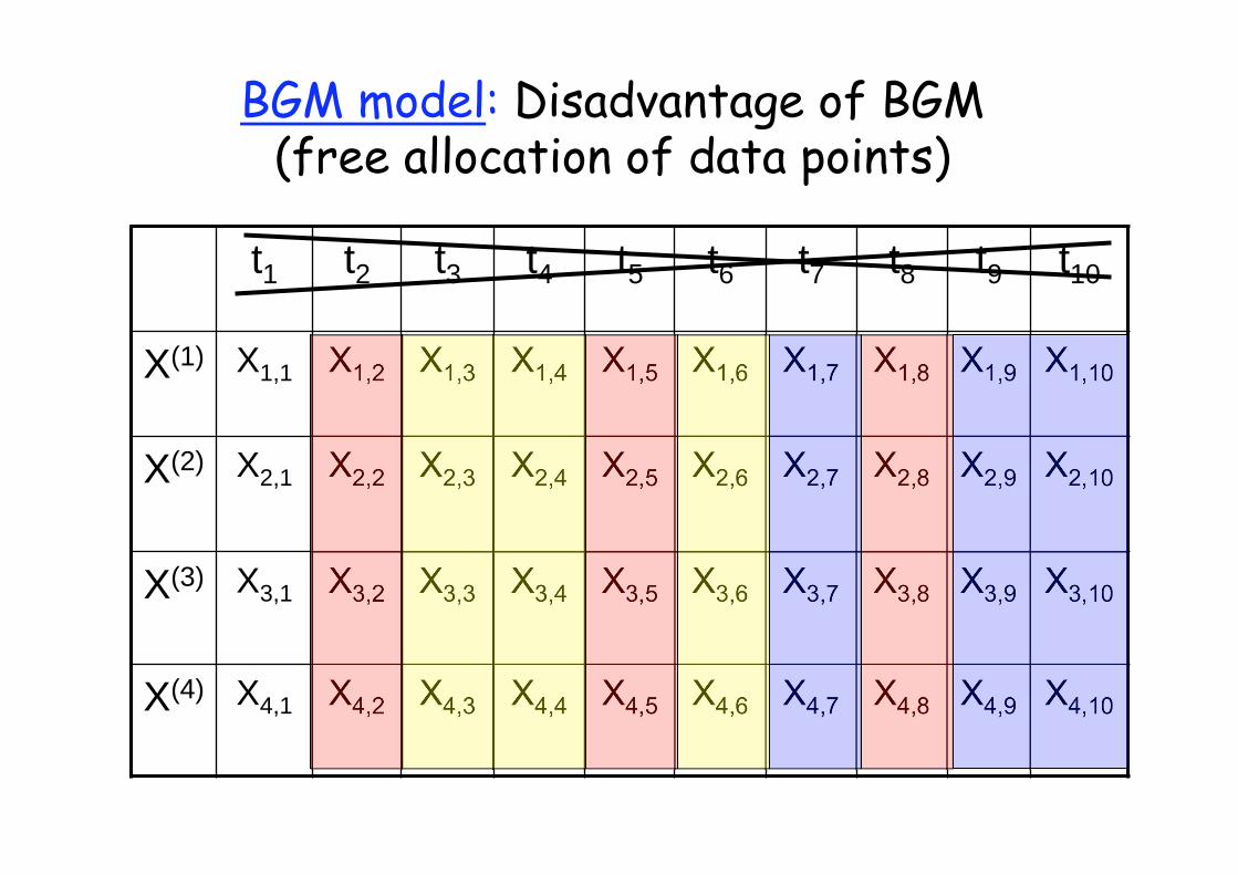
BGM model: Disadvantage of BGM (free allocation of data points)

1 2 2 1 2 3 1 3 3

X(1) X1,1 X1,2 X1,3 X1,4 X1,5 X1,6 X1,7 X1,8 X1,9 X1,10

X(2) X2,1 X2,2 X2,3 X2,4 X2,5 X2,6 X2,7 X2,8 X2,9 X2,10

X(3) X3,1 X3,2 X3,3 X3,4 X3,5 X3,6 X3,7 X3,8 X3,9 X3,10

X(4) X4,1 X4,2 X4,3 X4,4 X4,5 X4,6 X4,7 X4,8 X4,9 X4,10

free individual allocation of each time point so that the time structure is Not taken into account

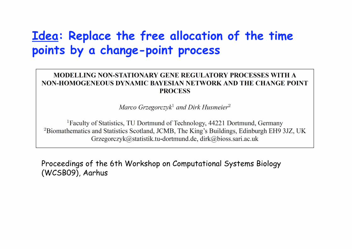
Idea: Replace the free allocation of the time points by a change-point process

Proceedings of the 6th Workshop on Computational Systems Biology (WCSB09), Aarhus

BGMD model (applicable to time series data)



data(j) consists of all observations allocated to component j



Poisson Change Point Process

Uniform BGe score

for each subset of data

BGMD model

t1 t2 t3 t4 t5 t6 t7 t8 t9 t10

X(1) X1,1 X1,2 X1,3 X1,4 X1,5 X1,6 X1,7 X1,8 X1,9 X1,10

X(2) X2,1 X2,2 X2,3 X2,4 X2,5 X2,6 X2,7 X2,8 X2,9 X2,10

X(3) X3,1 X3,2 X3,3 X3,4 X3,5 X3,6 X3,7 X3,8 X3,9 X3,10

X(4) X4,1 X4,2 X4,3 X4,4 X4,5 X4,6 X4,7 X4,8 X4,9 X4,10

Instead of free individual allocation of each time point

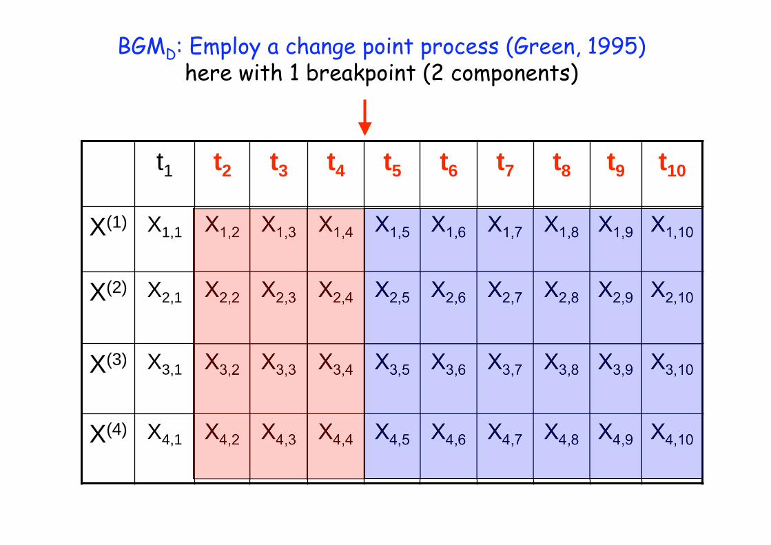
t1 t2 t3 t4 t5 t6 t7 t8 t9 t10

X(1) X1,1 X1,2 X1,3 X1,4 X1,5 X1,6 X1,7 X1,8 X1,9 X1,10

X(2) X2,1 X2,2 X2,3 X2,4 X2,5 X2,6 X2,7 X2,8 X2,9 X2,10

X(3) X3,1 X3,2 X3,3 X3,4 X3,5 X3,6 X3,7 X3,8 X3,9 X3,10

X(4) X4,1 X4,2 X4,3 X4,4 X4,5 X4,6 X4,7 X4,8 X4,9 X4,10

BGMD: Employ a change point process (Green, 1995) here with 1 breakpoint (2 components)

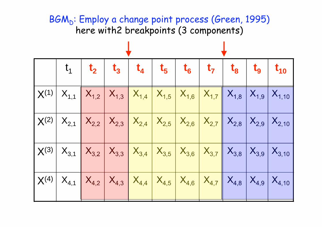
t1 t2 t3 t4 t5 t6 t7 t8 t9 t10

X(1) X1,1 X1,2 X1,3 X1,4 X1,5 X1,6 X1,7 X1,8 X1,9 X1,10

X(2) X2,1 X2,2 X2,3 X2,4 X2,5 X2,6 X2,7 X2,8 X2,9 X2,10

X(3) X3,1 X3,2 X3,3 X3,4 X3,5 X3,6 X3,7 X3,8 X3,9 X3,10

X(4) X4,1 X4,2 X4,3 X4,4 X4,5 X4,6 X4,7 X4,8 X4,9 X4,10

BGMD: Employ a change point process (Green, 1995) here with2 breakpoints (3 components)

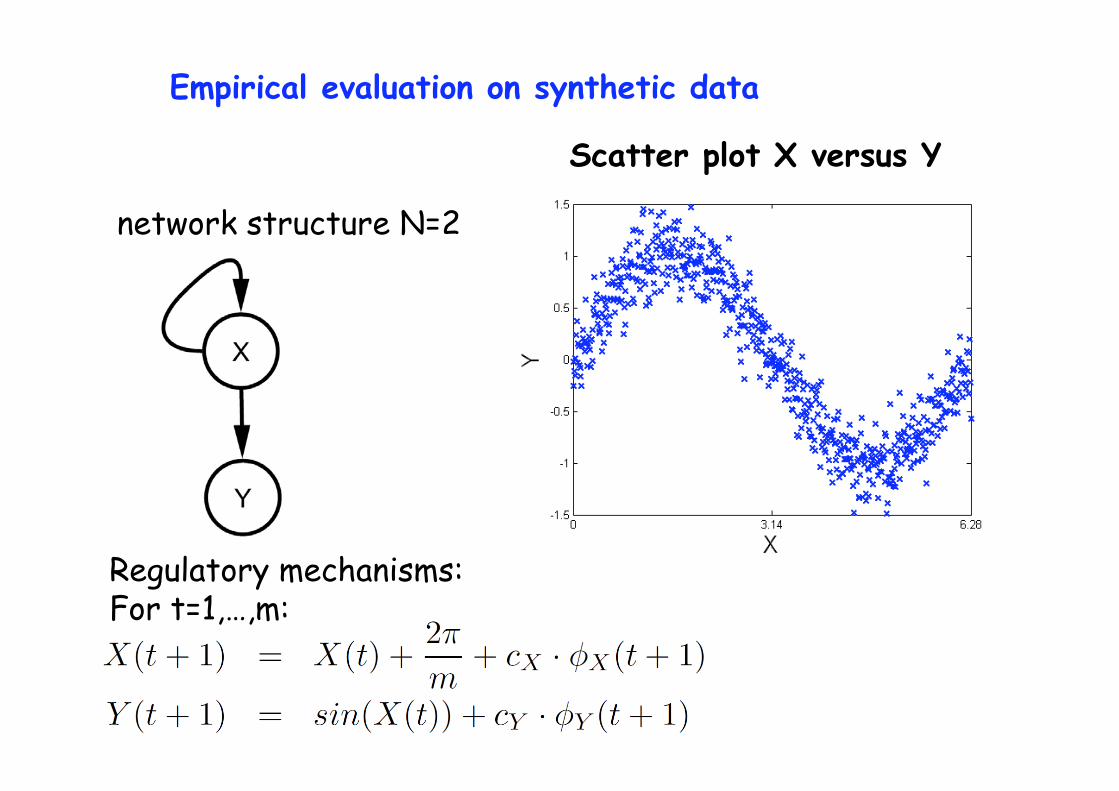
Empirical evaluation on synthetic data

Scatter plot X versus Y

network structure N=2

Regulatory mechanisms: For t=1,…,m:

Empirical evaluation on synthetic data

AUC histograms


BGe BGM BGMD

Regulatory mechanisms: For t=1,…,m:

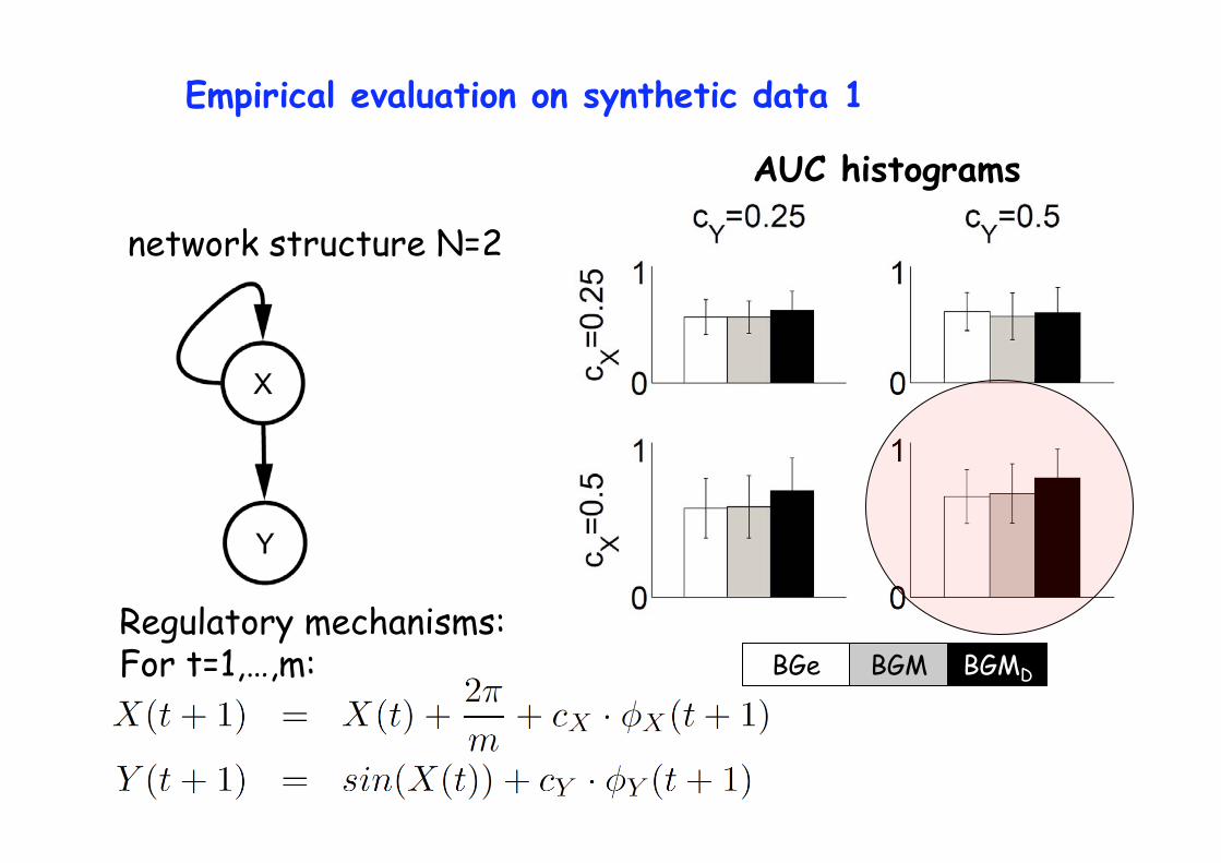
Empirical evaluation on synthetic data 1

AUC histograms


Regulatory mechanisms: For t=1,…,m: BGe BGM BGMD

Edge posterior probabilities cX=0.5 and cY=0.5

X X X Y Y Y Y X

Collaboration with the Institute of Molecular Plant

Sciences at Edinburgh University

2 time series T20 and T28 of microarray gene expression data from Arabidopsis thaliana.

- Focus on: 9 circadian genes: LHY, CCA1, TOC1, ELF4,

ELF3, GI, PRR9, PRR5, and PRR3

- Both time series measured under constant light condition


- Plants entrained with different light:dark cycles

10h:10h (T20) and 14h:14h (T28)

Circadian rhythms in Arabidopsis thaliana

Connectivity structures Heatmatrix representations

E.g.: T20,2h time series

BGM BGMD

White strong connectivity, Black no connection





4.1 BGM

4.2 BGMD

4.3 BGMD,2

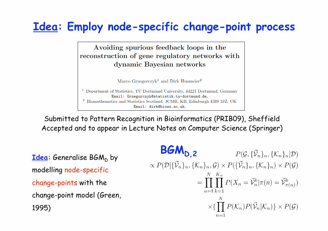
Submitted to Pattern Recognition in Bioinformatics (PRIB09), Sheffield Accepted and to appear in Lecture Notes on Computer Science (Springer)

Idea: Generalise BGMD by

modelling node-specific

change-points with the

change-point model (Green,

1995)

BGMD,2

Idea: Employ node-specific change-point process

t1 t2 t3 t4 t5 t6 t7 t8 t9 t10

X(1) X1,1 X1,2 X1,3 X1,4 X1,5 X1,6 X1,7 X1,8 X1,9 X1,10

X(2) X2,1 X2,2 X2,3 X2,4 X2,5 X2,6 X2,7 X2,8 X2,9 X2,10

X(3) X3,1 X3,2 X3,3 X3,4 X3,5 X3,6 X3,7 X3,8 X3,9 X3,10

X(4) X4,1 X4,2 X4,3 X4,4 X4,5 X4,6 X4,7 X4,8 X4,9 X4,10

Standard dynamic Bayesian network: homogeneous model

t1 t2 t3 t4 t5 t6 t7 t8 t9 t10

X(1) X1,1 X1,2 X1,3 X1,4 X1,5 X1,6 X1,7 X1,8 X1,9 X1,10

X(2) X2,1 X2,2 X2,3 X2,4 X2,5 X2,6 X2,7 X2,8 X2,9 X2,10

X(3) X3,1 X3,2 X3,3 X3,4 X3,5 X3,6 X3,7 X3,8 X3,9 X3,10

X(4) X4,1 X4,2 X4,3 X4,4 X4,5 X4,6 X4,7 X4,8 X4,9 X4,10

Heterogeneous dynamic Bayesian network BGM

t1 t2 t3 t4 t5 t6 t7 t8 t9 t10

X(1) X1,1 X1,2 X1,3 X1,4 X1,5 X1,6 X1,7 X1,8 X1,9 X1,10

X(2) X2,1 X2,2 X2,3 X2,4 X2,5 X2,6 X2,7 X2,8 X2,9 X2,10

X(3) X3,1 X3,2 X3,3 X3,4 X3,5 X3,6 X3,7 X3,8 X3,9 X3,10

X(4) X4,1 X4,2 X4,3 X4,4 X4,5 X4,6 X4,7 X4,8 X4,9 X4,10

Heterogeneous dynamic Bayesian network BGMD

Heterogenous dynamic Bayesian network with node-specific breakpoints BGMD,2

t1 t2 t3 t4 t5 t6 t7 t8 t9 t10

X(1) X1,1 X1,2 X1,3 X1,4 X1,5 X1,6 X1,7 X1,8 X1,9 X1,10

X(2) X2,1 X2,2 X2,3 X2,4 X2,5 X2,6 X2,7 X2,8 X2,9 X2,10

X(3) X3,1 X3,2 X3,3 X3,4 X3,5 X3,6 X3,7 X3,8 X3,9 X3,10

X(4) X4,1 X4,2 X4,3 X4,4 X4,5 X4,6 X4,7 X4,8 X4,9 X4,10

N=4 network structure

Overlaid scatter plots X(t) vs. Y(t+1) & X(t) vs. W(t+1) & X(t) vs. Z(t+1)

BGe BGMD BGMD,2

AUC histograms

School of Biological Sciences, Edinburgh University

2 time series T20 and T28 of microarray gene expression data from Arabidopsis thaliana:

- both time series measured under constant light condition


- plants entrained with different light:dark cycles

10h:10h (T20,2h) and 14h:14h (T28,2h)

2 new time series T24,4h and T24,4h of microarray gene expression data from Arabidopsis thaliana:

- both time series measured under constant light condition at 11/12 time points: 0h, 4h,…, 40h (44h)

- Focus on: 9 circadian genes: LHY, CCA1, TOC1, ELF4, ELF3, GI, PRR9, PRR5, and PRR3

BGMD,2 inference on Arabidopsis data

Gene expression time series plots (T20,2h, T28,2h, T24,4h and T24,4h)

LHY TOC1 CCA1

ELF4 ELF3 GI

PRR9 PRR5 PRR3

Idea: Merge the 4 time series to one single time series

whereby it has to be taken into account that there is no relation between the last time point of a time series

and the first time point of the next time series!

Time scale varies hours

For example: LHY

Node-specific posterior probabilities of transitions

Node-specific connectivity structures (heat matrices)

Average overall connectivity structure (as heat matrix)

Extracted network

…which has not been evaluated biologically (properly) yet…

Thank you for your

attention!

Any questions?

bayesian networks and their applications in systems biology · bayesian networks and their...

Documents