bayesian network representation - cedar.buffalo.edusrihari/cse674/chap3/3.1-bn... · • two random...

Machine Learning Srihari

1

Bayesian Network Representation

Sargur Srihari [email protected]


Topics

•  Exploiting Independence Properties •  Knowledge Engineering

2


Parameters for Independent r.v.s

•  Each Xi represents outcome of toss of coin i– Assume coin tosses are marginally independent –  i.e., (Xi ⊥Xj), therefore

P(X1,..,Xn)=P(X1)P(X2)..P(Xn)•  If we use standard parameterization of the joint

distribution, the independence structure is obscured and required 2n parameters

•  However we can use a more natural set of parameters: n parameters θ1,..θn 3


Conditional Parameterization •  Ex: Company is trying to hire recent graduates •  Goal is to hire intelligent employees

– No way to test intelligence directly – But have access to Student’s SAT score

•  Which is informative but not fully indicative

•  Two random variables –  Intelligence: Val(I)={i1,i0}, high and low – Score: Val(S)={s1,s0}, high and low

•  Joint distribution has 4 entries Need three parameters

4


Alternative Representation: Conditional Parameterization

•  P(I, S) = P(I)P(S | I)– Representation more compatible with causality

•  Intelligence influenced by Genetics, upbringing •  Score influenced by Intelligence

•  Note: BNs are not required to follow causality but they often do

•  Need to specify P(I) and P(S|I)

– Three binomial distributions (3 parameters) needed •  One marginal, two conditionals P(S|I=i0), P(S|i=i1) 5

Intelligence

SAT Grade SAT

Intelligence

(a) (b)


Conditional Parameterization and Conditional Independences •  Conditional Parameterization is combined

with Conditional Independence assumptions to produce very compact representations of high dimensional probability distributions

6

Machine Learning Srihari Naïve Bayes Model

•  Conditional Parameterization combined with Conditional Independence assumptions – Val(G)={g1, g2, g3} represents grades A, B, C

•  SAT and Grade are independent given Intelligence (assumption)

•  Knowing intelligence, SAT gives no information about class grade

•  Assertions •  From probabilistic reasoning •  From assumption

– Combining

7

Intelligence

SAT Grade SAT

Intelligence

(a) (b)

Three binomials, two 3-value multinomials: 7 params More compact than joint distribution

P(G|I)


BN for General Naiive Bayes Model

8

Class

X2X1 Xn. . .

P(C,X1,..Xn ) = P(C) P(Xi |C)i=1

n

∏

Encoded using a very small number of parameters Linear in the number of variables


Application of Naiive Bayes Model

•  Medical Diagnosis – Pathfinder expert system for lymph node

disease (Heckerman et.al., 1992) •  Full BN agreed with human expert 50/53

cases •  Naiive Bayes agreed 47/53 cases

9


“Student” Bayesian Network

10

•  Represents joint probability distribution over multiple variables •  BNs represent them in terms of graphs and conditional probability

distributions(CPDs) •  Resulting in great savings in no of parameters needed


Example of Probability Query

•  Posterior Marginal Estimation: P(I=i1|L=l0,S=s1)=? •  Probability of Evidence: P(L=l0,s=s1)=?

–  Here we are asking for a specific probability rather than a full distribution

12

P(Y = yi | E = e) = P(Y = yi ,E = e)P(E = e)

Probability of Evidence Posterior Marginal


Computing the Probability of Evidence

13

P(L,S) = P(D, I ,G,L,S)D, I ,G∑

= P(D)D, I ,G∑ P(I )P(G | D, I )P(L |G)P(S | I )

P(L = l0 , s = s1) = P(D)P(I )P(G | D, I )P(L = l0 |G)P(S = s1 | I )D, I ,G∑

P(E = e) = P(Xi | pa(Xi )) |E=ei=1

n

∏X \E∑

•  An intractable problem •  #P complete

•  Tractable when tree-width is less than 25 •  Most real-world applications have higher tree-width

•  Approximations are usually sufficient (hence sampling) •  When P(Y=y|E=e)=0.29292, approximation yields 0.3

Probability Distribution of Evidence

Probability of Evidence

More Generally

Sum Rule of Probability

From the Graphical Model


14

Genetic Inheritance and Bayesian Networks


15

Genetics Pedigree Example

•  One of the earliest uses of Bayesian Networks – Before general framework was defined

•  Local independencies are intuitive •  Model transmission of certain properties

such as blood type from parent to child


Phenotype and Genotype

•  Some background on genetics needed to model properly

•  Blood type is an observable quantity that depends on the genetic makeup – Called a phenotype

•  Genetic makeup of a person is called a genotype

16


17 17

Actual Electron Photomicrograph

Single Chromosome: ~108 base-pairsGenome: sequence of 3x109 base-pairs (nucleotides A,C,G,T) Represents full set of chromosomes

Genome has 46 chromosomes (22 are repeated plus XX and XY)

Large portions of DNA have no survival function (98.5%) and have variations useful for identification

TH01 is a location on short arm of chromosome 11:short tandem repeats (STR) of same base pair AATGVariant forms (alleles) different for different individuals

locus

DNA Basics


Genetic Model •  Human genetic material

– 22 pairs of autosomal chromosomes – One pair of sex chromosomes (X and Y)

•  Each chromosome contains genetic material that determine person’s properties

•  Locus: Region of chromosome of interest – Blood type is a particular locus

•  Alleles: Variants of locus – Blood type has three variants: A, B, O

18


Independence Assumptions

•  Arise from biology •  Once we know

– Genotype of a person •  additional evidence about other members of family

will not provide new information about blood-type – Genotype of both parents

•  Determine what is passed to off-spring •  Additional ancestral information not needed

•  These independencies can be captured in BN for a family tree 19


A small family tree

20

Harry


BN for Genetic Inheritance

21

G: Genotype B: Blood Type


Autosomal Chromosome •  In each pair,

– Paternal: inherited from father – Maternal: inherited from mother

•  Person’s genotype is an ordered pair (X,Y) –  with each having three possible values (A,B,O) –  there are nine values such as (A,B)

•  Blood type phenotype is a function of both copies – E.g., genotype (A,O) blood type is A –  (O,O) à O

22


CPDs for Genetic Inheritance

•  Penetrance Model P(B(c)|G(c)) – Probabilities of different phenotypes given

person’s genotype •  Deterministic for bloodtype

•  Transmission Model P(G(c)|G(p),G(m)) – Each parent equally likely to transmit either of

two alleles to child •  Genotype Priors P(G(c))

– Genotype frequencies in population 23


Real models more complex

•  Phenotypes for late-onset diseases are not a deterministic function of genotype – A particular genotype may have a higher

probability of a disease •  Genetic makeup of individual determined

by many genes •  Some phenotypes depend on many genes •  Multiple phenotypes depend on many

genes 24


Modeling multi-locus inheritance

•  Inheritance patterns of different genes not independent of each other

•  Need to take into account adjacent loci •  Introduce selector variables S(l,c,m)

•  1 if locus l in c’s maternal chromosome inherited from c’s maternal grandmother

•  2 if locus inherited from c’s maternal grandfather

•  Model correlations of variables of adjacent loci l and l’

25


Use of Genetic Inheritance Model

•  Extensively used in 1. In genetic counseling and prediction 2. In linkage analysis

26


Genetic Counseling and Prediction

•  Take phenotype with known loci and observed phenotype and genotype data for individuals –  to infer genotype and phenotype for another

person (planned child) •  Genetic data

– Direct measurements of relevant disease loci or nearby loci which are correlated with disease loci

27


Linkage Analysis •  Harder task •  Identifying disease genes from pedigree data

using several pedigrees – Several individuals exhibit disease phenotype – Available data

•  Phenotype information for many individuals in pedigree •  Genotype information for known location in chromosome

– Use inheritance model to evaluate likelihood – Pinpoint area linked to disease to further analyze

genes in that area •  Allows focusing on 1/10,000 of genome 28


Sparse BN in genetic inheritance

•  Allow reasoning about large pedigree and multiple loci

•  Allow use of model learning algorithms to understand recombination rates in different regions and penetration probabilities for different diseases

29


Graphs and Distributions

•  Relating two concepts: –  Independencies in distributions –  Independencies in graphs

•  I-Map is a relationship between the two

30


31

Independencies in a Distribution

•  Let P be a distribution over X •  I(P) is set of conditional independence

assertions of the form (X⊥Y|Z) that hold in P

X Y P(X,Y) x0 y0 0.08 x0 y1 0.32 x1 y0 0.12 x1 y1 0.48

X and Y are independent in P, e.g., P(x1)=0.48+0.12=0.6 P(y1)=0.32+0.48=0.8 P(x1,y1)=0.48=0.6x0.8 Thus (X⊥Y|ϕ)∈I(P)


Independencies in a Graph

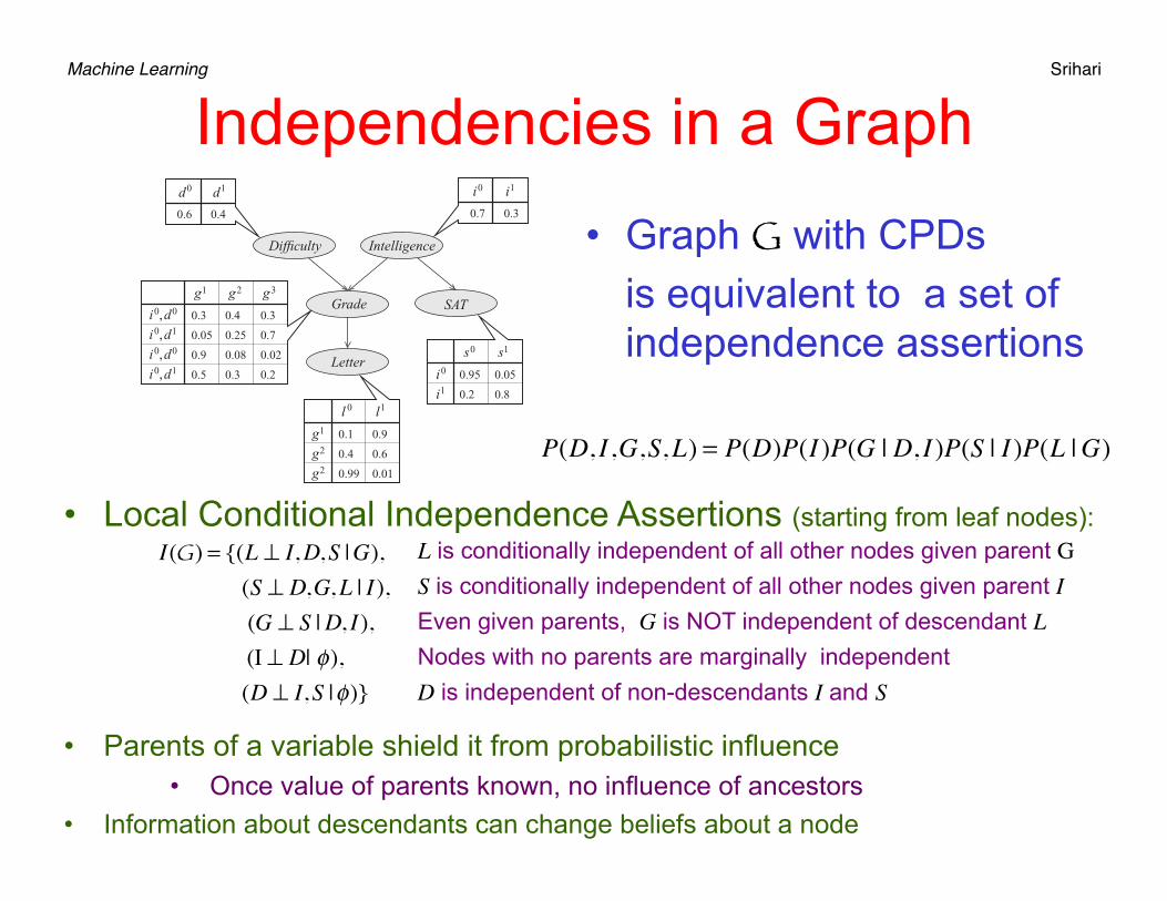
•  Local Conditional Independence Assertions (starting from leaf nodes):

•  Parents of a variable shield it from probabilistic influence •  Once value of parents known, no influence of ancestors

•  Information about descendants can change beliefs about a node


•  Graph G with CPDs is equivalent to a set of independence assertions

I(G) = {(L ⊥ I,D,S |G), (S ⊥ D,G,L | I ), (G ⊥ S |D, I ), (I ⊥ D| φ), (D ⊥ I,S |φ)}

Grade

Letter

SAT

IntelligenceDifficulty

d1d0

0.6 0.4

i1i0

0.7 0.3

i0

i1

s1s0

0.95

0.2

0.05

0.8

g1

g2

g2

l1l 0

0.1

0.4

0.99

0.9

0.6

0.01

i0,d0

i0,d1

i0,d0

i0,d1

g2 g3g1

0.3

0.05

0.9

0.5

0.4

0.25

0.08

0.3

0.3

0.7

0.02

0.2

L is conditionally independent of all other nodes given parent GS is conditionally independent of all other nodes given parent IEven given parents, G is NOT independent of descendant LNodes with no parents are marginally independent D is independent of non-descendants I and S


I-MAP •  Let G be a graph associated with a set of

independencies I(G) •  Let P be a probability distribution with a set

of independencies I(P) •  Then G is an I-map of I if I(G)⊆I(P) •  From direction of inclusion

– distribution can have more independencies than the graph

– Graph does not mislead in independencies existing in P

33


Example of I-MAP X

Y

X Y P(X,Y) x0 y0 0.08 x0 y1 0.32 x1 y0 0.12 x1 y1 0.48

X Y P(X,Y) x0 y0 0.4 x0 y1 0.3 x1 y0 0.2 x1 y1 0.1

X

Y

X

Y

G0 encodes X⊥Y or I(G0)={X⊥Y}

G1 encodes no Independence or I(G1)={Φ}

G2 encodes no Independence I(G2)={Φ}

X and Y are independent in P, e.g., G0 is an I-map of P G1 is an I-map of P G2 is an I-map of P

X and Y are not independent in P Thus (X⊥Y) \∈ I(P)

G0 is not an I-map of P G1 is an I-map of P G2 is an I-map of P

If G is an I-map of P then it captures some of the independences, not all


I-map to Factorization

•  A Bayesian network G encodes a set of conditional independence assumptions I(G)

•  Every distribution P for which G is an I-map should satisfy these assumptions – Every element of I(G) should be in I(P)

•  This is the key property to allowing a compact representation

35


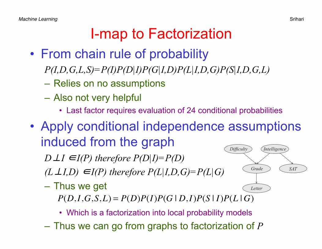
I-map to Factorization •  From chain rule of probability P(I,D,G,L,S)=P(I)P(D|I)P(G|I,D)P(L|I,D,G)P(S|I,D,G,L)

–  Relies on no assumptions –  Also not very helpful

•  Last factor requires evaluation of 24 conditional probabilities

•  Apply conditional independence assumptions induced from the graph D⊥I ∈I(P) therefore P(D|I)=P(D) (L⊥I,D) ∈I(P) therefore P(L|I,D,G)=P(L|G) –  Thus we get

•  Which is a factorization into local probability models

–  Thus we can go from graphs to factorization of P


Grade

Letter

SAT



Factorization to I-map •  We have seen that we can go from the

independences encoded in G, i.e., I (G), to Factorization of P

•  Conversely, Factorization according to G implies associated conditional independences –  If P factorizes according to G then G is an I-map for P–  Need to show that if P factorizes according to G then I(G)

holds in P–  Proof by example

37


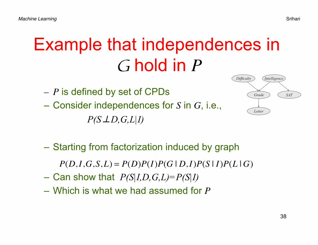
Example that independences in G hold in P

–  P is defined by set of CPDs –  Consider independences for S in G, i.e.,

P(S⊥D,G,L|I)

–  Starting from factorization induced by graph

–  Can show that P(S|I,D,G,L)=P(S|I) –  Which is what we had assumed for P

38


Grade

Letter

SAT


Machine Learning Srihari Perfect Map

•  I-map –  All independencies in I(G) present in I(P)–  Trivial case: all nodes interconnected

•  D-Map –  All independencies in I(P) present in I(G)–  Trivial case: all nodes disconnected

•  Perfect map –  Both an I-map and a D-map –  Interestingly not all distributions P over a given

set of variables can be represented as a perfect map

•  Venn Diagram where D is set of distributions that can be represented as a perfect map

I(G)={}

I(G)={A⊥B,C}

P

D

bayesian network representation - cedar.buffalo.edusrihari/cse674/chap3/3.1-bn... · • two random...

Documents