bayesian, mcmc, and multilevel modeling (a foray into … · introductionprior distributionsmcmc...
TRANSCRIPT

Introduction Prior distributions MCMC MCMCglmm
Bayesian, MCMC, and Multilevel Modeling(a foray into the subjective)
Christopher David Desjardinshttp://cddesjardins.wordpress.com
27 April 2010

Introduction Prior distributions MCMC MCMCglmm
Outline
1 Introduction
2 Prior distributions
3 MCMC
4 MCMCglmm

Introduction Prior distributions MCMC MCMCglmm
Bayesian toolbox for multilevel modeling
MCMC softwareJAGS. JAGS is cross-platform, actively developed, and can becalled directly from R via the rjags library. It can run anymodel as long as you can program it!
It is CLI only
WinBUGS and/or OpenBUGS for PC. OpenBUGS is supposedlycross-platform. Similar to JAGS but more tested and with alarge, active support community.
Can use with R via R2WinBUGS, BRugs
R software
MCMCglmm. This can do LMM and GLMM, meta-analyses,and more. Excellent vignette! Also Jarrod Hadfield is supernice!!!glmmAK. Longitudinal ordinal regression.MCMC diagnostics, the coda package.
CRAN task view: Bayesian!

Introduction Prior distributions MCMC MCMCglmm
Thomas Bayes
A Presbyterian minister with an itch for gambling, who now restsin Bunhill Fields.
Introduction Prior distributions MCMC MCMCglmm
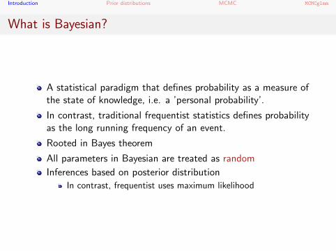
What is Bayesian?
A statistical paradigm that defines probability as a measure ofthe state of knowledge, i.e. a ’personal probability’.
In contrast, traditional frequentist statistics defines probabilityas the long running frequency of an event.
Rooted in Bayes theorem
All parameters in Bayesian are treated as random
Inferences based on posterior distribution
In contrast, frequentist uses maximum likelihood
Introduction Prior distributions MCMC MCMCglmm
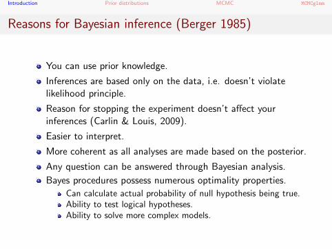
Reasons for Bayesian inference (Berger 1985)
You can use prior knowledge.
Inferences are based only on the data, i.e. doesn’t violatelikelihood principle.
Reason for stopping the experiment doesn’t affect yourinferences (Carlin & Louis, 2009).
Easier to interpret.
More coherent as all analyses are made based on the posterior.
Any question can be answered through Bayesian analysis.
Bayes procedures possess numerous optimality properties.
Can calculate actual probability of null hypothesis being true.Ability to test logical hypotheses.Ability to solve more complex models.
Introduction Prior distributions MCMC MCMCglmm
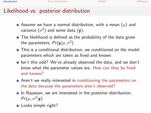
Likelihood vs. posterior distribution
Assume we have a normal distribution, with a mean (µ) andvariance (σ2) and some data (y).
The likelihood is defined as the probability of the data giventhe parameters, Pr(y|µ, σ2)
This is a conditional distribution, we conditioned on the modelparameters which are taken as fixed and known.
Isn’t this odd? We’ve already observed the data, and we don’tknow what the parameter values are. How can they be fixedand known?
Aren’t we really interested in conditioning the parameters onthe data because the parameters aren’t observed?
In Bayesian, we are interested in the posterior distribution,Pr(µ, σ2|y)
Looks simple right?

Introduction Prior distributions MCMC MCMCglmm
Bayes theorem
Mathematically
Pr(µ, σ2|y) = Pr(y|µ,σ2)Pr(µ,σ2)Pr(y)
Conceptually
Posterior = Likelihood∗PriorMarginal
Fortunately for us it simplifies ... a little
Pr(µ, σ2|y) ∝ Pr(y|µ, σ2)Pr(µ, σ2)
So ... what is the elephant in the room?

Introduction Prior distributions MCMC MCMCglmm
The elephant is ...
Prior distribution
Pr(µ, σ2)
Why?What is this?How do we handle this?How do we get rid of this?Do we want to get rid of this?Does it have any use?Does it have any harm?How can we marginalize this?Is it useful?

Introduction Prior distributions MCMC MCMCglmm
Oh what a prior!
Bayes thereom, and by extension Bayesian, forces us toincorporate priors
Priors can be very useful
Imagine your study is only one of a 1000 studies on topic X.You can formally synthesize all these results into your models.Gives you a ’stronger model’ because it’s based on 1000+1studies not just 1!?!Is it cheating?Philsophically, doesn’t science build on science? Our veryhypotheses on previous studies? Our models and our data arenot isolated, objective icebergs!

Introduction Prior distributions MCMC MCMCglmm
Oh no ... what a prior!
If our results are truly unique and we incorporate previousdata into our priors we might not see this in our results.
Priors are subjective!
With a small sample size, priors have a large effect on ourresults.
Choice of your priors can have a profound impact on yourinferences
MLE estimates are ’more objective’
Aren’t economists Bayesian? Oh no ...

Introduction Prior distributions MCMC MCMCglmm
Oh wait ... it is a wonderful prior!
Confession: I would describe myself as a subjective Bayesian!
I believe priors should be informative and guide our models.Bayesian is accepted in ecology.However, I’m not foolish!
Priors need to be based on sound evidence and must bejustifiable.
When in doubt, use non-informative, uniform priors
Estimates are similar to MLE in most instances.
Guess what ... you’re already using Bayesian!
Estimation of random effects in longitudinal analyses andHLM, BIC, IRT!

Introduction Prior distributions MCMC MCMCglmm
The legendary R. A. Fischer on probability
“The probability of any event is the ratio between thevalue at which an expectation depending on thehappening of the event ought to be computed, and thevalue of the thing expected upon its happening.” (InAldrich, 2008)
But then again, Fischer didn’t believe smoking caused cancer.

Introduction Prior distributions MCMC MCMCglmm
How can prior distributions affect our results?
Let’s take a look at rjags> require(rjags)
> dat0 <- na.omit(dat0)
> N <- nrow(dat0)
> Y <- dat0$ACT_ENGL
> x <- dat0$ACT_MATH
> dump(list=c("N","Y","x"),file="lr.data")
> datalr <- read.data(file="lr.data",format="jags")
> datalr
$x
[1] 14 19 26 15 19 18 17 13 15 16 22 21 19 18 19 16 19 20 22 25 21 19 21 12 18
[26] 21 20 20 26 21 21 24 20 20 22 23 17 18 20 19 16 19 15 29 26 17 18 20 17 16
[51] 20 17 16 15 17 16 28 20 25 22 26 18 25 18 22 19 26
$Y
[1] 16 25 24 21 17 13 18 19 16 19 17 19 15 23 21 20 16 22 18 18 14 19 22 10 13
[26] 21 18 18 16 18 24 28 25 16 16 17 14 15 18 22 15 18 10 23 19 22 20 21 16 19
[51] 18 15 12 16 19 19 27 16 23 16 23 19 25 19 25 19 20
$N
[1] 67

Introduction Prior distributions MCMC MCMCglmm
Exploring priors
> print(m1 <- jags.model(file="lr8920prior1.bug",data=datalr))
Compiling model graph
Resolving undeclared variables
Allocating nodes
Graph Size: 197
JAGS model:
model {
for (i in 1:N) {
Y[i] ~ dnorm(mu[i], tau)
mu[i] <- alpha + beta * (x[i] - x.bar)
}
x.bar <- mean(x)
alpha ~ dnorm(0.0, 1.0E-4)
beta ~ dnorm(0.0, 1.0E-4)
sigma <- 1.0/sqrt(tau)
tau ~ dgamma(1.0E-3, 1.0E-3)
}
Fully observed variables:
N Y x

Introduction Prior distributions MCMC MCMCglmm
What do these priors look like?
Priors on intercept and slope
rnorm(100, 0, 1/sqrt(1e−04))
Fre
quen
cy
−200 −100 0 100 200
05
1015
2025
Priors on variance
rgamma(100, shape = 0.001, scale = 0.001)
Fre
quen
cy
0e+00 2e−06 4e−06 6e−06 8e−06
020
4060
8010
0
Introduction Prior distributions MCMC MCMCglmm
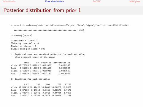
Posterior distribution from prior 1
> prior1 <- coda.samples(m1,variable.names=c("alpha","beta","sigma","tau"),n.iter=5000,thin=10)
|**************************************************| 100%
> summary(prior1)
Iterations = 10:5000
Thinning interval = 10
Number of chains = 1
Sample size per chain = 500
1. Empirical mean and standard deviation for each variable,
plus standard error of the mean:
Mean SD Naive SE Time-series SE
alpha 18.73395 0.42902 0.0191865 0.0221243
beta 0.51495 0.12166 0.0054406 0.0051588
sigma 3.42628 0.63731 0.0285015 0.0247560
tau 0.08829 0.01595 0.0007132 0.0006959
2. Quantiles for each variable:
2.5% 25% 50% 75% 97.5%
alpha 17.82418 18.47420 18.7603 18.98205 19.5555
beta 0.27909 0.44618 0.5155 0.58573 0.7579
sigma 2.88946 3.19051 3.3846 3.59386 4.0401
tau 0.06127 0.07742 0.0873 0.09824 0.1198

Introduction Prior distributions MCMC MCMCglmm
Maximum likelihood estimates
> coef(lm(Y ~ 1 + x))
(Intercept) x
8.5493151 0.5172069
The posterior distribution estimate of the slope is nearly identicalto the maximum likelihood estimate. But the intercept is a littledifferent. What happens if we decrease the variance?
Introduction Prior distributions MCMC MCMCglmm
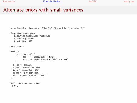
Alternate priors with small variances
> print(m2 <- jags.model(file="lr8920prior2.bug",data=datalr))
Compiling model graph
Resolving undeclared variables
Allocating nodes
Graph Size: 197
JAGS model:
model {
for (i in 1:N) {
Y[i] ~ dnorm(mu[i], tau)
mu[i] <- alpha + beta * (x[i] - x.bar)
}
x.bar <- mean(x)
alpha ~ dnorm(0.0, 100)
beta ~ dnorm(0.0, 100)
sigma <- 1.0/sqrt(tau)
tau ~ dgamma(1.0E-3, 1.0E-3)
}
Fully observed variables:
N Y x

Introduction Prior distributions MCMC MCMCglmm
What do these alternate priors look like?
Priors on intercept and slope
rnorm(100, 0, 1/sqrt(100))
Fre
quen
cy
−0.3 −0.2 −0.1 0.0 0.1 0.2 0.3
05
1015
20
I bet this will have an enormous impact!
Introduction Prior distributions MCMC MCMCglmm
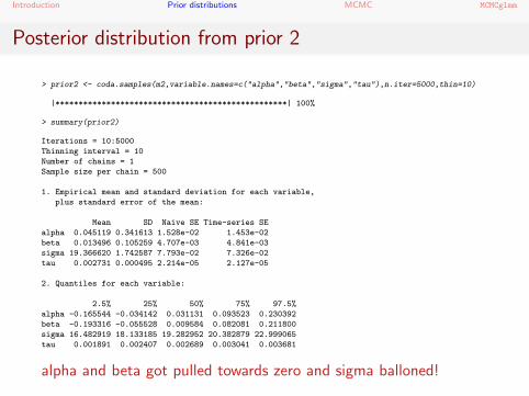
Posterior distribution from prior 2
> prior2 <- coda.samples(m2,variable.names=c("alpha","beta","sigma","tau"),n.iter=5000,thin=10)
|**************************************************| 100%
> summary(prior2)
Iterations = 10:5000
Thinning interval = 10
Number of chains = 1
Sample size per chain = 500
1. Empirical mean and standard deviation for each variable,
plus standard error of the mean:
Mean SD Naive SE Time-series SE
alpha 0.045119 0.341613 1.528e-02 1.453e-02
beta 0.013496 0.105259 4.707e-03 4.841e-03
sigma 19.366620 1.742587 7.793e-02 7.326e-02
tau 0.002731 0.000495 2.214e-05 2.127e-05
2. Quantiles for each variable:
2.5% 25% 50% 75% 97.5%
alpha -0.165544 -0.034142 0.031131 0.093523 0.230392
beta -0.193316 -0.055528 0.009584 0.082081 0.211800
sigma 16.482919 18.133185 19.282952 20.382879 22.999065
tau 0.001891 0.002407 0.002689 0.003041 0.003681
alpha and beta got pulled towards zero and sigma balloned!
Introduction Prior distributions MCMC MCMCglmm
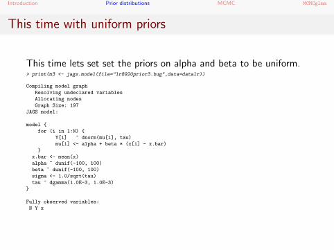
This time with uniform priors
This time lets set set the priors on alpha and beta to be uniform.> print(m3 <- jags.model(file="lr8920prior3.bug",data=datalr))
Compiling model graph
Resolving undeclared variables
Allocating nodes
Graph Size: 197
JAGS model:
model {
for (i in 1:N) {
Y[i] ~ dnorm(mu[i], tau)
mu[i] <- alpha + beta * (x[i] - x.bar)
}
x.bar <- mean(x)
alpha ~ dunif(-100, 100)
beta ~ dunif(-100, 100)
sigma <- 1.0/sqrt(tau)
tau ~ dgamma(1.0E-3, 1.0E-3)
}
Fully observed variables:
N Y x
Introduction Prior distributions MCMC MCMCglmm
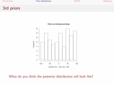
3rd priors
Priors on intercept and slope
runif(100, min = −100, max = 100)
Fre
quen
cy
−100 −50 0 50 100
02
46
810
1214
What do you think the posterior distribution will look like?
Introduction Prior distributions MCMC MCMCglmm
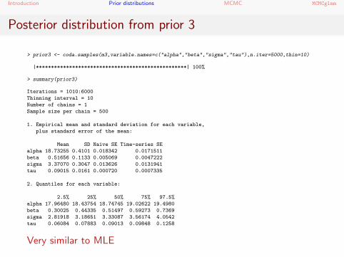
Posterior distribution from prior 3
> prior3 <- coda.samples(m3,variable.names=c("alpha","beta","sigma","tau"),n.iter=5000,thin=10)
|**************************************************| 100%
> summary(prior3)
Iterations = 1010:6000
Thinning interval = 10
Number of chains = 1
Sample size per chain = 500
1. Empirical mean and standard deviation for each variable,
plus standard error of the mean:
Mean SD Naive SE Time-series SE
alpha 18.73255 0.4101 0.018342 0.0171511
beta 0.51656 0.1133 0.005069 0.0047222
sigma 3.37070 0.3047 0.013626 0.0131941
tau 0.09015 0.0161 0.000720 0.0007335
2. Quantiles for each variable:
2.5% 25% 50% 75% 97.5%
alpha 17.96480 18.43754 18.74745 19.02622 19.4980
beta 0.30025 0.44335 0.51497 0.59273 0.7369
sigma 2.81918 3.18651 3.33087 3.56174 4.0542
tau 0.06084 0.07883 0.09013 0.09848 0.1258
Very similar to MLE
Introduction Prior distributions MCMC MCMCglmm
Your turn to run priors!
I’d like you guys to break up into groups of 3.
Using my code and data, tweak the model, and run it!
Run jags.model() then coda.samples()
Try it with a few different priors and repeat the process
for the same priors.
What were your priors? How did they affect your estimates?Do you get the same estimates when you ran the same priorsagain? What if you used set.seed()?
Introduction Prior distributions MCMC MCMCglmm
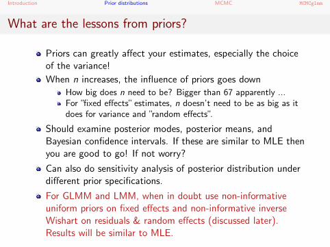
What are the lessons from priors?
Priors can greatly affect your estimates, especially the choiceof the variance!
When n increases, the influence of priors goes down
How big does n need to be? Bigger than 67 apparently ...For ”fixed effects” estimates, n doesn’t need to be as big as itdoes for variance and ”random effects”.
Should examine posterior modes, posterior means, andBayesian confidence intervals. If these are similar to MLE thenyou are good to go! If not worry?
Can also do sensitivity analysis of posterior distribution underdifferent prior specifications.
For GLMM and LMM, when in doubt use non-informativeuniform priors on fixed effects and non-informative inverseWishart on residuals & random effects (discussed later).Results will be similar to MLE.

Introduction Prior distributions MCMC MCMCglmm
How do we estimate posterior distributions?
Recall for a simple linear regressioen of a normally distributedvariable...
Bayes Theorem
Pr(µ, σ2|y) ∝ Pr(y|µ, σ2)Pr(µ, σ2)
In order to calculate the posterior distribution often requiresintegrating out many variables, taking integrals of integrals.
Imagine the case of a GLMM, where you have to estimate yourfixed effects, variances, and random effects.This can not be derived analytically and requiresapproximation.
MCMC provides a way to estimate the posterior distribution.
It can ”find” the posterior distribution within MCMC error.
MCMC works by walking stochastically through space, theMonte Carlo part, and hopefully from areas of low to highprobability of where our parameters are living.

Introduction Prior distributions MCMC MCMCglmm
Starting values
The first thing that you need for MCMC are starting values
This will help to speed up convergence and reduce wastedwandering
All estimated parameters require starting values
These may be generated by the program
Or supplied by the user
Using the MLE, when possible, is a good way to start MCMC

Introduction Prior distributions MCMC MCMCglmm
Metropolis-Hastings
After we’ve initialized our chain we need to decide where togo next and start sampling from our posterior distribution!
To do this we generate a candidate destination and decidewhether we should move there or stay put.
One way to do this is using a Metropolis-Hastings (MH)algorithm.
During the first iteration, a random set of coordinates arepicked from a multivariate normal distribution and comparedto the intial coordinates.
If the posterior probability is greater for the new coordinates,than we move to the new coordinates.

Introduction Prior distributions MCMC MCMCglmm
Metropolis-Hastings continued
If the posterior probability is lower, than we may stay or wemay go.
Once this iteration is complete, we repeat this again with ourcoordinates at the end of the last iteration becoming our baseline coordinates.
We repeat this over and over again depending upon how manyiterations we’ve specified.
Iterations are saved and we examine them when we look atthe posterior distribution.
Pros: Easy to write your own algorithms, less mathematical
Cons: Very slow to converge!

Introduction Prior distributions MCMC MCMCglmm
MH conceptually

Introduction Prior distributions MCMC MCMCglmm
Gibbs sampling
A special case of MH
In MH, we could move in multiple directions simulatenously,i.e. we moved for both µ and σ2.
However, we could have moved in just one direction at a time,for example move in the direction of µ conditioned on somevalue of σ2 say 1.
Mathematically then, Pr(µ|σ2 = 1, y)

Introduction Prior distributions MCMC MCMCglmm
Gibbs sampling continued
First, let’s move in the direction of µ conditioned on somevalue of σ2
We could generate a new candidate randomly and ask if it’sposterior probability is higher but ...
We often know the equation for this conditional distribution,this is Gibbs Sampling
We know we’re at σ2 = 1, so why don’t we just calculate µdirectly.
Repeat this process for σ2 conditioning on the new value of µand so on.
Pro: Converges much faster!
Cons: Much more difficult to program .. so let’s let MCMCglmmor JAGS do the work!

Introduction Prior distributions MCMC MCMCglmm
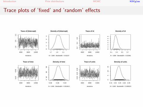
MCMC diagnostics - How do we know it’s working right?
First thing you should look at our trace plots.
They should be free from patternEach plot should have roughly a horizontal line with noascending/descending pattern
Next you should look at autocorrelation between iterations.
Iterations have a tendency to be autocorrelated and are notindependent.Should examine this empirically and thin out your chain.
There are lots of helpful diagnostic tools in the coda package
raftery.diag() - Tells you how many MCMC iterations youneed to run for convergencegeweke.diag() - Compares means from first part of Markovchain with the last part.
Burn, burn, burn, thin, thin, thin

Introduction Prior distributions MCMC MCMCglmm
Other MCMC issues
Researchers have reported that MCMC needs some time to’warm’ up to remove autocorrelation, i.e. to reachconvergence.
This is specified as the burn-in time.
You run MCMC but do not store the output until after theburn-in periodgelman.diag() in coda is one way to help you determine thelength of the required burn-in until convergenceHowever, the need for burn-in is debatable.
Many MCMC programs allow you to specify multiple chains(up to 5).
MCMCglmm uses only one.Crossing chains indicate convergence.

Introduction Prior distributions MCMC MCMCglmm
MCMCglm
MCMCglmm (Hadfield, 2010) is one library in R that can beused to run generalized linear mixed models.
MCMCglmm can run Guassian, Binomial, Poisson, Zero-InflatedPoisson, Ordinal, Multinomial, and other models.
I came about MCMCglmm when I had longitudinal data that waszero-inflated and could not be estimated with lme4.
Specification of models in MCMCglmm() is very similar toglmer() and lmer().
However, you need to specify priors.

Introduction Prior distributions MCMC MCMCglmm
Pros/Cons MCMCglmm
Pros
Can estimate very complex models.Lots of diagnostic tools available via coda package.
Bayesian outshines traditional statistics here.
Developer extremely helpful and active on r-sig-mixed
models mailing list.Can calculate actual p-values, 95% Bayesian confidenceintervals, Deviance information criterion.
Cons
Very slow with large data sets. My data set can take 24 hoursto run!Requires specification of priors and starting valuesDoesn’t give frequentist p-values, no t-valueA little harder to program than lme4

Introduction Prior distributions MCMC MCMCglmm
Specifying a MCMCglmm() model
Default arguments to MCMCglmm()
MCMCglmm(fixed, random=NULL, rcov= units, family=”gaussian”, mev=NULL, data,start=NULL, prior=NULL,
tune=NULL, pedigree=NULL, nodes=”ALL”, scale=TRUE, nitt=13000, thin=10, burnin=3000, pr=FALSE,
pl=FALSE, verbose=TRUE, DIC=TRUE, singular.ok=FALSE, saveX=FALSE, saveZ=FALSE, slice=FALSE)
fixed and random fixed and random effects formulae; rcovresidual Cov structure; family probability family; mev specifymeasurement error (meta-analysis); data data; start startingvalues; prior the priors; tune Cov matrix for proposed latentvariable; pedigree, nodes, and scale useful for genetics; nitt # ofiterations; thin thinning interval; burnin # of burn-ins; pr and plsave posterior of random effects and latent variables; verbose getoutput; DIC Deviance information criterion; singular.ok whenfalse linear dependencies in fixed effects are removed; saveX andsaveZ save fixed effects and random effects matrix; slice use slicesampling (type of MCMC).

Introduction Prior distributions MCMC MCMCglmm
Labdosage data set
We’ll use the labdosage.txt file. I believe you all are familiar withit?
> head(dos)
id group time count
1.1 1 2mg 1 5
1.2 1 2mg 2 2
1.3 1 2mg 3 2
1.4 1 2mg 4 5
1.5 1 2mg 5 2
1.6 1 2mg 6 4
Introduction Prior distributions MCMC MCMCglmm
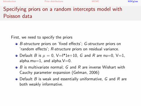
Specifying priors on a random intercepts model withPoisson data
First, we need to specify the priors
B-structure priors on ’fixed effects’; G-structure priors on’random effects’; R-structure priors on residual variance.
Default B is µ = 0, V=I*1e+10, G and R are nu=0, V=1,alpha.mu=1, and alpha.V=0.
B is multivariate normal; G and R are inverse Wishart withCauchy parameter expansion (Gelman, 2006)
Default B is weak and essentially uniformative, G and R areboth weakly informative.

Introduction Prior distributions MCMC MCMCglmm
Specifying a random intercepts model continued
> prior<-list(R=list(V=1, nu=0.002), G=list(G1=list(V=1, nu=0.002)))
These are essentially the same priors used for the the JAGS model.
> m1 <- MCMCglmm(count ~ 1 + time, random=~id, prior=prior,family="poisson",
data=dos)
MCMC iteration = 0
Acceptance ratio for latent scores = 0.000396
MCMC iteration = 1000
Acceptance ratio for latent scores = 0.424758
....................
MCMC iteration = 13000
Acceptance ratio for latent scores = 0.391338
Introduction Prior distributions MCMC MCMCglmm
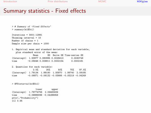
Summary statistics - Fixed effects
> # Summary of 'Fixed Effects'
> summary(m1$Sol)
Iterations = 3001:12991
Thinning interval = 10
Number of chains = 1
Sample size per chain = 1000
1. Empirical mean and standard deviation for each variable,
plus standard error of the mean:
Mean SD Naive SE Time-series SE
(Intercept) 1.93977 0.080995 0.0025613 0.0030749
time -0.05646 0.006811 0.0002154 0.0002181
2. Quantiles for each variable:
2.5% 25% 50% 75% 97.5%
(Intercept) 1.78134 1.88190 1.93970 1.99740 2.09185
time -0.06871 -0.06132 -0.05666 -0.05219 -0.04249
> HPDinterval(m1$Sol)
lower upper
(Intercept) 1.78774756 2.09483939
time -0.06889096 -0.04286956
attr(,"Probability")
[1] 0.95
Introduction Prior distributions MCMC MCMCglmm
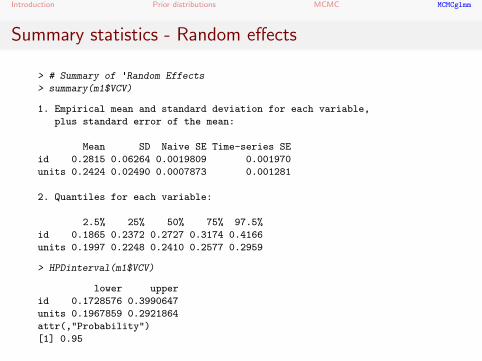
Summary statistics - Random effects
> # Summary of 'Random Effects
> summary(m1$VCV)
1. Empirical mean and standard deviation for each variable,
plus standard error of the mean:
Mean SD Naive SE Time-series SE
id 0.2815 0.06264 0.0019809 0.001970
units 0.2424 0.02490 0.0007873 0.001281
2. Quantiles for each variable:
2.5% 25% 50% 75% 97.5%
id 0.1865 0.2372 0.2727 0.3174 0.4166
units 0.1997 0.2248 0.2410 0.2577 0.2959
> HPDinterval(m1$VCV)
lower upper
id 0.1728576 0.3990647
units 0.1967859 0.2921864
attr(,"Probability")
[1] 0.95
Introduction Prior distributions MCMC MCMCglmm
Trace plots of ’fixed’ and ’random’ effects
4000 8000 12000
1.8
2.0
2.2
Iterations
Trace of (Intercept)
1.7 1.9 2.1
01
23
4
N = 1000 Bandwidth = 0.02157
Density of (Intercept)
4000 8000 12000
−0.
07−
0.05
Iterations
Trace of time
−0.08 −0.06 −0.04
010
3050
N = 1000 Bandwidth = 0.001813
Density of time
4000 8000 12000
0.2
0.4
0.6
Iterations
Trace of id
0.1 0.3 0.5 0.7
01
23
45
6
N = 1000 Bandwidth = 0.01592
Density of id
4000 8000 12000
0.20
0.25
0.30
Iterations
Trace of units
0.15 0.20 0.25 0.30 0.35
05
1015
N = 1000 Bandwidth = 0.006523
Density of units

Introduction Prior distributions MCMC MCMCglmm
Autocorrelations of iterations
> autocorr(m1$Sol)
, , (Intercept)
(Intercept) time
Lag 0 1.00000000 -0.49419125
Lag 10 0.08802531 -0.07252791
Lag 50 0.06445487 -0.04806522
Lag 100 -0.02629911 0.06327561
Lag 500 0.03672346 -0.04482030
, , time
(Intercept) time
Lag 0 -0.49419125 1.00000000
Lag 10 0.02048099 0.04815938
Lag 50 -0.04384447 0.03041308
Lag 100 -0.01538620 -0.03313733
Lag 500 -0.00999942 0.02657281

Introduction Prior distributions MCMC MCMCglmm
How does this compare with glmer()
> m1.glmer <- glmer(count ~ 1 + time + (1 | id), family="poisson",data=dos)
Effect MCMCglmm lme4
Intercept 1.9398 2.0389Time -0.0565 -0.0546id 0.2815 0.2652
Very similar! This is great! Additionally, the standard errors weresimilar too with MCMCglmm being slightly smaller.
Introduction Prior distributions MCMC MCMCglmm
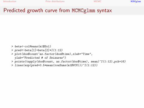
Predicted growth curve from MCMCglmm syntax
> beta<-colMeans(m1$Sol)
> pred<-beta[1]+beta[2]*I(1:12)
> plot(dos$count~as.factor(dos$time),xlab="Time",
ylab="Predicted # of Seizures")
> points(tapply(dos$count, as.factor(dos$time), mean)~I(1:12),pch=16)
> lines(exp(pred+0.5*mean(rowSums(m1$VCV)))~I(1:12))

Introduction Prior distributions MCMC MCMCglmm
Predicted growth curve
●
●
●
●
●
●
● ●●
●
●
●
●
●
●
●
●
●
●
●
●
●
●
●●
●
●
●
●
●
●
●
●
●
●
●
●
●
1 2 3 4 5 6 7 8 9 10 11 12
05
1015
2025
3035
Time
Pre
dict
ed #
of S
eizu
res
●
●●
●
●
●
●● ●
●● ●

Introduction Prior distributions MCMC MCMCglmm
Random slopes MCMCglmm model
> m2 <- MCMCglmm(count ~ 1 + time, random=~id + time, prior=prior,
family="poisson",data=dos, verbose=FALSE)
Which model is better: Random intercepts or random slope?
> m1$DIC;m2$DIC
[1] 3871.923
[1] 3861.976

Introduction Prior distributions MCMC MCMCglmm
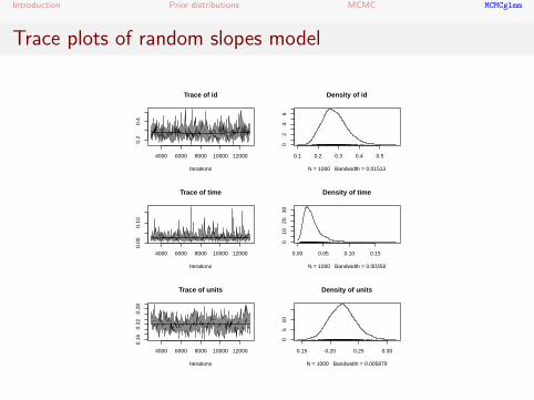
Random slopes model
> summary(m2$VCV)
1. Empirical mean and standard deviation for each variable,
plus standard error of the mean:
Mean SD Naive SE Time-series SE
id 0.28073 0.05920 0.0018722 0.0022649
time 0.02867 0.01890 0.0005977 0.0007020
units 0.22134 0.02244 0.0007097 0.0009372
2. Quantiles for each variable:
2.5% 25% 50% 75% 97.5%
id 0.181775 0.24027 0.27404 0.31639 0.41390
time 0.007685 0.01663 0.02452 0.03464 0.07818
units 0.180095 0.20586 0.22075 0.23545 0.26900
Introduction Prior distributions MCMC MCMCglmm
Trace plots of random slopes model
4000 6000 8000 10000 12000
0.2
0.4
Iterations
Trace of id
0.1 0.2 0.3 0.4 0.5
02
46
N = 1000 Bandwidth = 0.01513
Density of id
4000 6000 8000 10000 12000
0.00
0.10
Iterations
Trace of time
0.00 0.05 0.10 0.15
010
2030
N = 1000 Bandwidth = 0.00358
Density of time
4000 6000 8000 10000 12000
0.16
0.22
0.28
Iterations
Trace of units
0.15 0.20 0.25 0.30
05
10
N = 1000 Bandwidth = 0.005879
Density of units

Introduction Prior distributions MCMC MCMCglmm
Random slopes model with a static predictor
> m3 <- MCMCglmm(count ~ 1 + time + group, random=~id + time,
prior=prior, family="poisson",data=dos,
verbose=FALSE)
> m2$DIC; m3$DIC
[1] 3861.976
[1] 3860.961

Introduction Prior distributions MCMC MCMCglmm
Summary statistics: Fixed effects
> summary(m3$Sol)
1. Empirical mean and standard deviation for each variable,
plus standard error of the mean:
Mean SD Naive SE Time-series SE
(Intercept) 2.05451 0.14353 0.0045389 0.0050984
time -0.05584 0.01520 0.0004808 0.0005261
group2mg -0.27097 0.14036 0.0044387 0.0043285
2. Quantiles for each variable:
2.5% 25% 50% 75% 97.5%
(Intercept) 1.75796 1.9676 2.05187 2.14983 2.33057
time -0.08692 -0.0651 -0.05606 -0.04607 -0.02599
group2mg -0.53615 -0.3666 -0.27407 -0.17733 0.00905
Introduction Prior distributions MCMC MCMCglmm
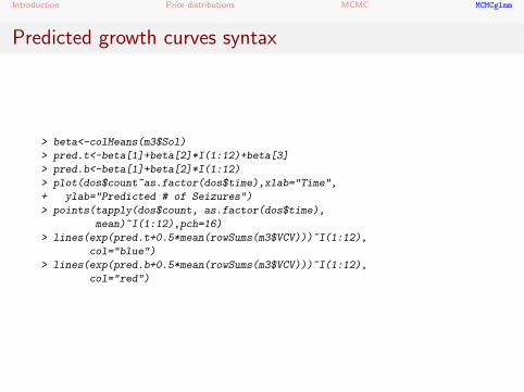
Predicted growth curves syntax
> beta<-colMeans(m3$Sol)
> pred.t<-beta[1]+beta[2]*I(1:12)+beta[3]
> pred.b<-beta[1]+beta[2]*I(1:12)
> plot(dos$count~as.factor(dos$time),xlab="Time",
+ ylab="Predicted # of Seizures")
> points(tapply(dos$count, as.factor(dos$time),
mean)~I(1:12),pch=16)
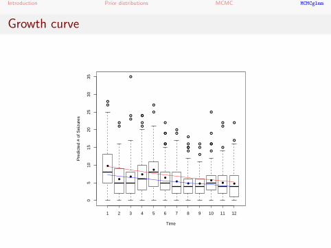
> lines(exp(pred.t+0.5*mean(rowSums(m3$VCV)))~I(1:12),
col="blue")
> lines(exp(pred.b+0.5*mean(rowSums(m3$VCV)))~I(1:12),
col="red")
Introduction Prior distributions MCMC MCMCglmm
Growth curve
●
●
●
●
●
●
● ●●
●
●
●
●
●
●
●
●
●
●
●
●
●
●
●●
●
●
●
●
●
●
●
●
●
●
●
●
●
1 2 3 4 5 6 7 8 9 10 11 12
05
1015
2025
3035
Time
Pre
dict
ed #
of S
eizu
res
●
●●
●
●
●
●● ●
●● ●
Introduction Prior distributions MCMC MCMCglmm
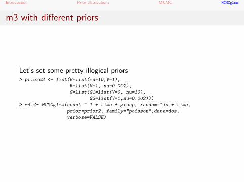
m3 with different priors
Let’s set some pretty illogical priors> priors2 <- list(B=list(mu=10,V=1),
R=list(V=1, nu=0.002),
G=list(G1=list(V=0, nu=10),
G2=list(V=1,nu=0.002)))
> m4 <- MCMCglmm(count ~ 1 + time + group, random=~id + time,
prior=prior2, family="poisson",data=dos,
verbose=FALSE)

Introduction Prior distributions MCMC MCMCglmm
And the results ...
Effects Uninformative priors Crazy priorsIntercept 2.055 2.061Time -0.056 -0.056Group -0.271 -0.270Random Intercept 0.264 0.266Random Slope 0.029 0.0274
With 780 data points, the likelihood already swamps the prior!

Introduction Prior distributions MCMC MCMCglmm
Running MCMCglmm() in your group
Spend some time now in a group running different priors anddifferent models on the data set.
Maybe try specifying starting values?
start <- list(B=2.05,-0.06,-0.27)
m3a <- MCMCglmm(count ∼ 1 + time + group,
random=∼id + time,family="poisson",data=dos,
prior=prior,start=start,verbose=FALSE)
I don’t recommend starting values for G and R
If you need help with syntax please ask.
Did you find anything interesting?

Introduction Prior distributions MCMC MCMCglmm
To Bayesian or not to Bayesian ...
In my opinion, it’s useful to know Bayesian methods as MLapproaches & least squares approaches don’t always work.
I believe that Bayesian methods will become more and moreimportant as computers become more and more powerful.
Bayesian frees you from the awkwardness of frequentiststatistics and creates the opportunity to include priorinformation.
But ... like everything there are costs to Bayesian.
Hopefully I’ve give you just enough information to bedangerous

Introduction Prior distributions MCMC MCMCglmm
Thanks!