bayesian information criterion for singular...

Bayesian Information Criterion for Singular Models

Mathias Drton

Department of StatisticsUniversity of Chicago → Washington

Joint work with an AIM group:Vishesh Karwa, Martyn Plummer, Aleksandra Slavkovic, Russ Steele

1 / 33

Outline

1 The Bayesian information criterion (BIC)

2 Singular models and ‘circular reasoning’

3 A proposal for a ‘singular BIC’

4 Examples

2 / 33

Bayesian information criterion (BIC)

Observe a sample Y1, . . . ,Yn

Parametric model M (set of probability distributions π)

Maximized log-likelihood function ˆ̀(M)

Bayesian information criterion (Schwarz, 1978)

BIC(M) := ˆ̀(M)− dim(M)

2log n

‘Generic’ model selection approach:

Maximize BIC(M) over set of considered models

3 / 33

Example: Linear regression

Observe n independent realizations of the ‘system’:

Y = ω1X1 + ω2X2 + ω3X3 + ε with ε ∼ N(0, σ2)

Models ≡ coordinate subspaces:

MJ = {ω ∈ R3 : ωj = 0 ∀j 6∈ J}, J ⊆ {1, 2, 3}.

Dimension |J| (or rather, |J|+ 1)

4 / 33

Linear regression (covariates i.i.d. N(0, 1), ω1 = 1, σ = 2)

5 / 33

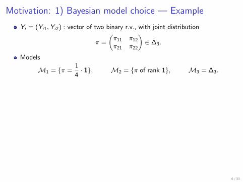
Motivation: 1) Bayesian model choice — Example

Yi = (Yi1,Yi2) : vector of two binary r.v., with joint distribution

π =

(π11 π12

π21 π22

)∈ ∆3.

Models

M1 = {π =1

4· 1}, M2 = {π of rank 1}, M3 = ∆3.

Prior on models, e.g.,

P(M1) = P(M2) = P(M3) =1

3.

Prior on π given model, e.g.,

P(π |M2) = distribution on rank 1 matrices in ∆3.

Data-generating process under distribution π from Mi :

P(Y1, . . . ,Yn |π,Mi ) =n∏

i=1

πyi1,yi2

6 / 33

Motivation: 1) Bayesian model choice

Posterior model probability in fully Bayesian treatment:

P(M|Y1, . . . ,Yn) ∝ P(M)︸︷︷︸prior

P(Y1, . . . ,Yn |M).

Marginal likelihood:

Ln(M) := P(Y1, . . . ,Yn |M)

=

∫P(Y1, . . . ,Yn |π,M)︸︷︷︸

likelihood fct.

d P(π |M)︸︷︷︸prior

7 / 33

Motivation: 2) Asymptotics

Y1, . . . ,Yn i.i.d. sample from a distribution π0 in a parametric model

M = {π(ω) : ω ∈ Rd}

Theorem (Schwarz, 1978; Haughton, 1988; and others)

Assume P(ω |M) is a ‘nice’ prior on Rd . Then in ‘nice’ models,

log Ln(M) = ˆ̀n(M)− d

2log(n) + Op(1),

and a better (Laplace) approximation to error Op

(n−1/2

)is possible.

Note:

The ‘model complexity term’ d2 log(n) does not depend on the true distribution π0.

8 / 33

Where asymptotics come from: In a regular model. . .

Gradient ∇`n(ω̂) = 0;

Hessian Hn(ω̂) of − 1n `n converges to positive definite matrix (w.p. 1).

Taylor approximation around MLE ω̂:

`n(ω) ≈ `n(ω̂) − n

2(ω − ω̂)>Hn(ω̂)(ω − ω̂)

Integral approximately Gaussian (‘nice’ prior):∫Rd

exp(`n(ω)

)· f (ω) dω

≈ exp(`n(ω̂)

)· f (ω̂) ·

∫Rd

exp(−n

2(ω − ω̂)>Hn(ω̂)(ω − ω̂)

)dω︸︷︷︸√(

2π

n

)d

· det (Hn(ω̂))−1

9 / 33

Consistency

TheoremFix a finite set of ‘nice’ models. Then, BIC selects a true model of smallestdimension with probability tending to one as n→∞.

Proof.

Finite set of models =⇒ pairwise comparisons suffice.

If P0 ∈M1 (M2 and d1 < d2, then

ˆ̀n(M2)− ˆ̀n(M1) = Op(1); and (d2 − d1) log n→∞.

If P0 ∈M1 \ clos(M2), then with probability tending to one,

1

n

[ˆ̀n(M1)− ˆ̀n(M2)

]> ε > 0; and log(n)/n→ 0.

10 / 33

Outline




4 Examples

11 / 33

Singular models

Model is singular if

‘approximation by a positive definite quadratic formnot possible everywhere’.

Examples:

I Reduced rank regressionI Gaussian mixture modelsI Any other mixture modelI Factor analysisI Hidden Markov modelsI Graphical models with latent variablesI . . .

12 / 33

Singular integrals

In R2, ‘the’ regular integral behaves like∫ 1

0

∫ 1

0

e−n(x2+y2) dx dy ∼ π

4· 1

n

An integral arising from a singular model could look like:∫ 1

0

∫ 1

0

e−nx2y2

dx dy ∼√π

2· log(n)

n1/2.

Proof:∫ 1

0

∫ 1

0

e−nx2y2

dx dy =

∫ 1

0

1

y√n

(∫ y√n

0

e−u2

du

)dy =

√π

2· 1√

n

∫ √n

0

erf(v)

vdv

=

√π

2· 1√

n[log(v)erf(v)]

√n

0 −1√n

∫ √n

0

log(v)e−v2

dv =

√π

2· log(n)

n1/2+O

(1√n

).

Substitution u = (y√n) · x , then v =

√n · y , then integration by parts.

13 / 33

Watanabe’s theorem

Theorem 6.7 in Watanabe (2009)

Suppose Y1, . . . ,Yn are drawn i.i.d. from a distribution π0 in a singular model M.Then, under ‘suitable technical conditions’, the marginal likelihood sequencesatisfies

log Ln(M) = ˆ̀n(M)− λ(π0) log(n) +

[m(π0)− 1

]log log(n) + Op(1).

Note:

The ‘model complexity term’ λ(π0) log(n)−[m(π0)− 1

]log log(n) generally

depends on the unknown true distribution π0.

14 / 33

How might we use mathematical knowledge. . . ?

Example: reduced rank regression

Parameter space{ matrices of rank ≤ H }

Model selection problem: Determine appropriate rank H

Singularities π0 correspond to matrices of rank < H (‘null set’)

Learning coefficient λ(π0) and its order m(π0) are functions of rank of π0.

‘Circular reasoning’

To define a truly Bayesian information criterion for singular models overcome:

Rank unknown −−−−−−−−−−→←−−−−−−−−−− Model complexity unknown

15 / 33

Outline




4 Examples

16 / 33

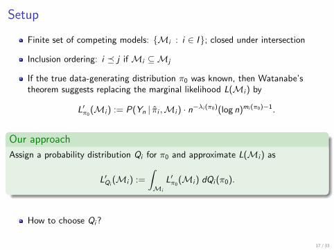
Setup

Finite set of competing models: {Mi : i ∈ I}; closed under intersection

Inclusion ordering: i � j if Mi ⊆Mj

If the true data-generating distribution π0 was known, then Watanabe’stheorem suggests replacing the marginal likelihood L(Mi ) by

L′π0(Mi ) := P(Yn | π̂i ,Mi ) · n−λi (π0)(log n)mi (π0)−1.

Our approach

Assign a probability distribution Qi for π0 and approximate L(Mi ) as

L′Qi(Mi ) :=

∫Mi

L′π0(Mi ) dQi (π0).

How to choose Qi?

17 / 33

Candidates for Qi — conditioning on Mi

Typically, it holds in an ‘almost surely’ sense that

λ(π0) =dim(Mi )

2, m(π0) = 1.

Hence, if π0 follows the posterior distribution given model Mi , that is,

Qi (π0) = P(π0 |Mi ,Yn)

then averaging wrto. Qi gives the standard BIC.

This choice of Qi does not reflect uncertainty wrto. models;condition solely on Mi .

18 / 33

Candidates for Qi — conditioning on Mi and submodels

We suggest choosing the posterior distribution for π0 given all submodels ofMi , that is,

Qi = P(π0 | {M : M⊆Mi},Yn) =

∑j�i P(π0 |Mj ,Yn)P(Mj |Yn)∑

j�i P(Mj |Yn).

The distribution Qi puts positive mass on submodels.(e.g., positive prob to rank 1 matrices when considering rank 2 matrices)

BUT: What about P(Mj |Yn)? These are the posterior prob’s we want toapproximate in the first place.

19 / 33

Recursive structure

Singular model selection problems typically have the following features:

The smallest model is regular.I Reduced rank regression: Rank 0I Latent class models: Independence of discrete r.v.I Factor analysis: Independence of normal r.v.I . . .

Learning coefficients (order) are ‘almost surely’ constant along submodels.Approximation at generic points in Mj ⊂Mi :

L′ij := P(Yn | π̂i ,Mi ) · n−λij (log n)mij−1 > 0.

I Reduced rank regression: matrices of lower rankI Latent class models: matrices of lower rankI Factor analysis: smaller # factorsI . . .

Recursive approach starting from the smallest model.

20 / 33

An equation system

For our proposed choice of Qi :

L′(Mi ) := L′Qi(Mi ) =

1∑j�i P(Mj |Yn)

·∑j�i

L′ij P(Mj |Yn)

=1∑

j�i L(Mj)P(Mj)·∑j�i

L′ij L(Mj)P(Mj).

Plugging-in approximations gives the equation system:

L′(Mi ) =1∑

j�i L′(Mj)P(Mj)·∑j�i

L′ij L′(Mj)P(Mj), i ∈ I .

21 / 33

Triangular system

Assume P(Mi ) ∝ const in the sequel.

Clearing denominators we obtain the triangular system:

L′(Mi )2 +

[(∑j≺i

L′(Mj))− L′ii

]· L′(Mi )−

∑j≺i

L′ij L′(Mj) = 0, i ∈ I .

For smallest model, the positive solution is

L′(Mi ) = L′ii > 0.

Equation system has unique positive solution.

Definition (Singular BIC)

sBIC(Mi ) = log L′(Mi ),

where (L′(Mi ) : i ∈ I ) solves the above equation system.

22 / 33

Properties

Reduces to ordinary BIC if models are regular

Consistency

Closer to behavior of Bayesian procedures

23 / 33

Outline




4 Examples

24 / 33

Reduced rank regression

Multivariate linear model for Y ∈ RN , with covariate X ∈ RM :

Y = CX + ε, ε ∼ N (0, IN).

Definition

Reduced rank regression model for rank 0 ≤ H ≤ min{M,N}:

Y ∼ N (CX , In ⊗ IN), C ∈ RN×M and rank(C ) ≤ H.

X1

L1

L2

X2

X3

Y3

Y4

Y1

Y2

Parameter space:

RN×MH :=

{C ∈ RN×M : rank(C ) ≤ H

}.

dim(RN×M

H

)= H(N + M − H).

Sing(RN×M

H

)= RN×M

H−1 .

25 / 33

Bayesian rank selection

Parametrization:

g : RN×H × RH×M → RN×MH

(B,A) 7→ BA.

I Maximal rank of the Jacobian of g :

dim(RN×M

H

)= H(N + M − H).

I Singularities of the map g (rank-deficient Jacobian):

(B,A) with either rank(B) < H or rank(A) < H.

Posterior distribution for rank (with priors P(H) and ψH(B,A)):

P(H | Y ) = P(H)

∫L(BA)ψH(B,A) d(B,A).

Learning coefficients −→ Aoyagi & Watanabe (2005)

26 / 33

Singular BIC in action (4/3, 1, 2/3, 0, . . . )

27 / 33

Singular BIC in action (5/4, 1, 3/4, 1/2, . . . )

28 / 33

Singular BIC in action (5/4, 1, 3/4, 1/2, . . . )

29 / 33

Univariate Gaussian mixtures

30 / 33

Factor analysis

31 / 33

More factor analysis

32 / 33

What do you think?

33 / 33

bayesian information criterion for singular...

Documents