Chapter 1

Bayesian Inference

(09/17/17)

A witness with no historical knowledge

There is a town where cabs come in two colors, yellow and red.1 Ninety percent of the cabs

are yellow. One night, a taxi hits a pedestrian and leaves the scene without stopping. The

skills and the ethics of the driver do not depend on the color of the cab. An out-of-town

witness claims that the color of the taxi was red. The out-of town witness does not know

the proportion of yellow and red cabs in the town and makes a report on the sole basis of

what he thinks he has seen. Since the accident occurred during the night, the witness is not

completely reliable but it has been assessed that such a witness makes a correct statement

is four out of five (whether the true color of the cab is yellow or red). How should one

use the information of the witness? Because of the uncertainty, we should formulate our

conclusion in terms of probabilities. Is it more likely then that a red cab was involved in

the accident? Although the witness reports red and is correct 80 percent of the time, the

answer is no.

Recall that there are many more yellow cabs. The red sighting can be explained either

by a yellow cab hitting the pedestrian (an event with high prior probability) which is

incorrectly identified (an event with low probability), or a red cab (with low probability)

which is correctly identified (with high probability). Both the prior probability of the event

and the precision of the signal have to be used in the evaluation of the signal. Bayes’ rule

1The example is adapted from Salop (1987)

1

2 Bayesian tools2

provides the method to compute probability updates. Let R be the event “a red cab is

involved”, and Y the event “a yellow cab is involved”. Likewise, let r (y) be the report “I

have seen a red (yellow) cab”. The probability of the event R conditional on the report r

is denoted by P (R|r). By Bayes’ rule,2

P (R|r) =P (r|R)P (R)

P (r)=

P (r|R)P (R)

P (r|R)P (R) + P (r|Y)(1− P (R)). (1.1)

The probability that a red cab is involved before hearing the testimony is P (R) = 0.10.

P (r|R) is the probability of a correct identification and is equal to 0.8. P (r|Y) is the

probability of an incorrect identification and is equal to 0.2. Hence,

P (R|r) =0.8× 0.1

0.8× 0.1 + 0.2× 0.9=

4

13<

1

2.

Note that this probability is much less than the precision of the witness, 80 percent, because

a “red” observation is more likely to come from a wrong identification of a yellow cab than

from a correct identification of a red cab.

The example reminds us of the difficulties that some people may have in practical cir-

cumstances. Despite these difficulties,3 all rational agents in this book are assumed to be

Bayesians. The book will concentrate only on the difficulties of learning from others by

rational agents.

A witness with historical knowledge

Suppose now that the witness is a resident of the town who knows that only 10 percent of

the cabs are red. In making his report, he tells the color which is the most likely according

to his rational deduction. If he applies the Bayesian rule and knows his probability of

making a mistake, he knows that a yellow cab is more likely to be involved. He will report

“yellow” even if he thinks that he has seen a red cab. If he thinks he has seen a yellow

one, he will also say “yellow”. His private information (the color he thinks he has seen) is

ignored in his report.

The omission of the witness’ information in his report does not matter if he is the only

witness and if the recipient of the report attempts to assess the most likely event: the

witness and the recipient of the report come to the same conclusion. But suppose there is

a second witness with the same sighting skill (correct 80 percent of the time) and who also

thinks he has seen a red cab. That witness who attempts to report the most likely event

2Using the definition of conditional probabilities, P (R|r)P (r) = P (R and r) = P (r|R)P (R).3The ability of people to use Bayes’ rule has been tested in experiments, with mixed results (Holt and

Anderson, 1993).

3 Bayesian tools3

says also “yellow”. The recipient of the two reports learns nothing from the reports. For

him the accident was caused by a yellow cab with a probability of 90 percent.

Recall that when the first witness came from out-of-town, he was not informed about the

local history and he gave an informative report, “red”. That report may be inaccurate,

but it provides information. Furthermore, it triggers more information from the second

witness. After the report of the first witness, the probability of R increased from 0.1 to

4/13. When that probability of 4/13 is conveyed to the second witness, he thinks that a

red car is more likely.4 He therefore reports “red”. The probability of the inspector who

hears the reports of the two witnesses is now raised to the level of the last (second) witness.

Looking for your phone as a Bayesian

You live in a two room apartment with two rooms, one that you keep orderly, one that

is messy. After stepped out with a friend, you realize that you have left your cell phone

behind. The phone is equally likely to be in one of the two rooms. You tell your friend:

please looking for my phone that I have left in the apartment while I fetch the car that is

parked in the next block. Your friend comes back without having found the phone. Which

room is the more probable for the phone. Answer before reading the next paragraph.

You may think that your friend has looked into the two rooms. In the orderly room, it is

harder to miss the phone. Therefore, no seeing the phone in that room makes it unlikely

(compared to the other room) that the phone is there. You increase the probability of the

messy room. You are a Bayesian.

In the formalization of this story, we can that there are two rooms 1 (orderly) and 2

(messy). There are two states of the nature: the phone is in room 1 or room 2. A search

in room i, i = 1 or 2 produces a signal that is 1 (finding the phone) or 0 (not finding the

phone. Each signal has a probability qi to be equal to 1 if the phone is in room i. The

probability of not finding the phone in room i when the phone is actually in room i is

1 − qi is positive. If the phone is in room 3 − i, (the room other than i), the signal si is

zero. When you do not find the phone in Room 1, you think, rationally, you increase your

probability that the phone is in Room 2. If you search in Room 2 for about the same time,

then you think that the probability of a mistaken signal s2 = 0 is higher than s1 = 0 if the

phone is in Room 1. Comparing the two rooms, you increase the probability of the phone

in Room 2. The precise Bayesian calculus will be done later in this chapter.

4Exercise: prove it.

4 Bayesian tools4

1.1 The standard Bayesian model

1.1.1 General remarks

The main issue is to learn about something. In the Bayesian framework, the “something”

is a possible fact, which can be called a state of nature. That fact may take place in the

future or it may already have taken place with an uncertain knowledge about it. Actually,

in a Bayesian framework, there is no difference between a future event and a past event

that are both uncertain. The future event may be “rain” or “shine”, to occur tomorrow.

For a Bayesian, nature chooses the weather today (with some probability, to be described

below), and that weather is realized tomorrow.

The list of possible states is fixed in Bayesian learning. There is no room for learning about

states that are not on the list of possible states before the learning process. That is an

important limitation of Bayesian learning. There is no ”unknown unknown”, to use the

famous characterization of secretary of state Rumsfeld, only “known unknown”. In other

words, one knows what is unknown.

The Bayesian process begins by putting weights on the unknowns, probabilities on the

possible states of nature. These probabilities may be objective, such as the probability of

“tail” or “face” in throwing a coin, but that is not important. What matters is that these

probabilities are the ones that the learner uses at the learning process. These probabilities

will be called belief. A “belief” will be a distribution of probabilities over the possible

states. By an abuse of language, a belief will sometimes be the probability of a particular

state, especially in the case of two possible states: the “belief” in one state will obviously

define the probability of the other state. The belief before the reception of information is

called the prior belief.

Learning is the processing of information that comes about the state. This information

comes in the form of a signal. Examples are the witness report of the previous section, a

weather forecast, an advice by a financial advisor, the action of some “other” individual,

etc... In order to be informative, that signal must depend on the state. But that signal is

imperfect and does not reveal exactly the state (otherwise there would be nothing inter-

esting to think about). A natural definition of a signal is therefore a random variable that

can take different values with some probabilities and the distribution of these probabilities

depend on the actual state. The processing of the information of the signal is the use of

the signal to update the prior belief into the posterior belief. That step is the core of the

Bayesian learning process and its mechanics are driven by Bayes’ rule. In that process,

the learner knows the mechanics of the signal, i.e., the probability of receiving a particular

signal value conditional on the true state. Bayes’ rule combines that knowledge with the

5 Bayesian tools5

prior distribution of the state to compute the posterior distribution.

Examples

1. The binary model

• States of nature θ ∈ Θ = {0, 1}

• Signal s ∈ {0, 1} with P (s = θ|θ) = qθ.

2. Financial advising (i.e., Value Line):

• States of nature: a stock will go up 10% or go down 10% (two states).,

• Advice {Strong Sell, Sell, Hold, Buy, Strong Buy}.

3. Gaussian signal:

• Two states of nature θ ∈ Θ = {0, 1}

• Signal s = θ+ ε, where s has a normal distribution with mean zero and variance

σ2.

4. Gaussian model:

• The state θ has a normal distribution with mean θ and variance sigma2θ.

• Signal s = θ+ ε, where s has a normal distribution with mean zero and variance

σ2ε .

Note how in all cases, the (probability) distribution of the signal depends on the state.

These are just examples and we will see later how each of them is a useful tool to address

specific issues. We begin with the simplest model, the binary model.

1.1.2 The binary model

In all models of rational learning that are considered here, there is a state of nature (or

just “state”) that is an element of a set. We will use the notation θ for this state. In the

previous story, the states R and Y can be defined by θ ∈ {0, 1} or θ ∈ {θ0, θ1}.

The sighting by the witness is equivalent to the reception of a signal s that can be 0 or

1. A signal that takes one of two value is called a binary signal. The uncertainty about

6 Bayesian tools6

States ofNature

Observation (signal)

s = 1 s = 0

θ = θ1 q1 1− q1

θ = θ0 1− q0 q0

Table 1.1.1: Binary signal

the sighting is represented by the assumption that s is the realization of a random variable

that depends on the true state. One possible dependence is given by Table 1.

Using the definition of conditional probability,

P (θ = 1|s = 1) =P (θ = 1 ∩ s = 1)

P (s = 1)=P (s = 1|θ = 1)P (θ = 1)

P (s = 1),

which yields Bayes’ rule

P (θ = 1|s = 1) =q1P (θ = 1)

q1P (θ = 1) + (1− q1)(1− P (θ = 1). (1.2)

The signal 1 is “good news” about the state 1 (it increases the belief in state 1), if and

only if q1 > 1− q0, or

q1 + q0 > 1.

A signal can be informative about a state because it is likely to occur in that state, with

q1. But one should be aware that it may be even more informative when it is very unlikely

to occur in the other state, when 1− q0 is low. If one is looking for piece of metal, a good

detector responds to an actual piece. But a better detector may be one that does not

respond at all when there is no metal in front of it.

When q1 = q0 = q, the signal is a symmetric binary signal (SBS) and in this case, we will

call q the precision of the signal. (The precision will have a different definition when the

signal is not a SBS). Note that q could be less than 1/2, in which case we could switch the

roles of s = 1 and s = 0. The inequality q > 1/2 is just a convention, which will be kept

here for any SBS.

Useful expressions of Bayes’ rule

The formula in (1.2) is unwieldy. When the space state is discrete, it is often more useful

to express Bayes’ rule in terms of likelihood ratio, i.e., the ratio between the probabilities

7 Bayesian tools7

of two states, hereafter LR. (There can be more than two states in the set of states). Here

we have only two states, but LR is also useful for any finite number of states, as will be

seen in the search application below.

P (θ = 1|s = 1)

P (θ = 0|s = 1)︸ ︷︷ ︸ =(P (s = 1|θ = 1)

P (s = 1|θ = 0)

)︸ ︷︷ ︸×

(P (θ = 1)

P (θ = 0)

)︸ ︷︷ ︸ . (1.3)

posterior LR signal factor prior LR

The signal factor depends only on the properties of the signal. With the specification of

Table 1,P (θ = 1|s = 1)

P (θ = 0|s = 1)=

q11− q0

× P (θ = 1)

P (θ = 0). (1.4)

The expression of Bayes’ rule in (1.3) is much simpler than the original formula because it

takes a multiplicative form that has a symmetrical look.

State one is more likely when the LR is greater than 1. In the previous example of the

car incident, say that “1” is “red”. The prior for red cab is 1/10. The signal factor

P (s = 1|θ = 1)/P (s = 1|θ = 0) (correct / mistake) is .8/0.2=4. It is not sufficient to

reverse the belief that yellow is more likely.

For some applications of rational learning, it will be convenient to transform the product

in the the previous equation into a sum, which is performed by the logarithmic function.

Denote by λ the prior Log likelihood ratio between the two states, and by λ′ is posterior,

after receiving the signal s. Bayes’ rule now takes the form

λ′ = λ+ Log(q1/(1− q0)). (1.5)

Both the multiplicative form in (1.3) and the additive form in (1.5) are especially when

there is a sequence of signal. For example, with two signals s1 and s2,

P (θ = 1|s1, s2)

P (θ = 0|s1, s2)=(P (s2|θ = 1)

P (s2|θ = 0)

)×(P (s1|θ = 1)

P (s1|θ = 0)

)×(P (θ = 1)

P (θ = 0)

).

One can repeat the updating for any number of signal observations. It is also obvious that

the final update does not depend on the order of the signal observations.

Bounded signals and belief updates

The signal takes here only two values and is therefore bounded. The same is true if the

number of signal values is more than two but finite. The implication is that values of the

8 Bayesian tools8

posterior probabilities cannot be arbitrarily close to one or zero. They are bounded away

from zero and one. This will have profound implications later one. At this stage, one can

just state that the binary signal (or any signal with finite values) is bounded.

1.1.3 Multiple binary signals: search on the sea floor

Some objects that have been lost at sea are extremely valuable and have stimulated many

efforts for their recovery: submarines, nuclear bombs dropped of the coast of Spain, airline

wrecks. In searching for the object under the surface of the sea, different informations

have been used: last sight of the object, surface debris, surveys of the area by detecting

instruments. The combination of these informations through Bayesian analysis led to the

findings of the USS Scorpion submarine (2009), the USS Central America with its treasure

(1857-1988), the wreck of AF 447 (2009-2011).

Assume that the search area is divided in N cells. The prior probability distribution is

such that wi is equal to the probability that the object is in cell i. Using previous notation,

wi = P (θ = θi). If the detector is passed over cell i, the probability of finding the object

is pi, which may depend on the cell because of variations in the conditions for detection

(depth, type of soil, etc..). The question is how after a fruitless search over an area, the

probability distribution is updated from w to w′. Let θi be the state that the wreck is in

cell i, and Z the event that no detection was made.

P (θ = θi|Z) =1

P (Z)P (Z|θ = θi)P (θ = θi).

P (Z|θ = θi) =

{1− pi, if there if the detector is passed over cell i,

1, if the detector is not passed over cell i.

Defining pi = 0 if there is no search in cell I (a search may not be over all the cells), the

posterior distribution is given by

w′i = A(1− pi)wi, with A =

1∑Ni=1(1− pi)wi

. (1.6)

An example: the search for AF447

In the early hours of June 1, 2009, with 228 passengers and crew, Air France Flight 447

disappeared in the celebrated “pot au noir”.5 No message had been sent by the crew but

both “black boxes”–they are red– were retrieved after a two years. They have provided a

5This part of the Intertropical Convergence Zone (ITCZ) between Brazil and Africa is well known toaviators. It has been a special challenge for all sailboats, merchant ships in the 19th century and racerstoday.

9 Bayesian tools9

gripping transcript of a failure of social learning in the cockpit during the last ten minutes

of the flight. We focus here on the learning process during the search for the wreck, 3000

meters below the surface of the ocean. It provides a fascinating example of information

gathering and learning.

First, a prior probability distribution (PD) has to be established. At each stage the proba-

bility distribution should orient the next search effort the result of which should be used to

update the PD, and so on. That at least is the theory. 6 It will turn out that the search for

AF447 did not follow the theory. Following Keller (2015), the search which lasted almost

two years before a complete success, proceeded in stages.

1. The aircraft had issued an automated signal on its position at regular time intervals.

From this, it was established that the object should be in a circle of 40 nautical

miles7 (nmi) centered at the last known position (LKP). That disk was endowed

with a probability distribution, hereafter PD, that was chosen to be uniform.

2. Previous studies on crashes for similar conditions showed a normal distribution

around the LKP with standard deviation of 8 nmi.

3. Five days after the crash, began a period during which debris were found, the first of

them about 40 nmi from the LKP. A numerical model was used for “back drifting”

to correct for currents and wind. That process, which is technical and beyond the

scope of this analysis, led to another PD.

4. The three previous probability distributions were averaged with weights of 0.35, 0.35

and 0.3, respectively. These weights are guesses and so far, the updating is not

Bayesian. It’s not clear how a Bayesian updating could have been done at this stage.

The PD is now the prior distribution represented in the panel A of Figure 1.1. The

Bayesian use of that PD will come only after Step 5.

5. Three different searches were conducted, with no result, between June and the end

of 2010.

(a) First, the black boxes of the aircraft are supposed to emit an audible sound for

forty days. That search for a beacon is represented in the panel B of Figure 1.1.

It produced nothing. There has been no Bayesian analysis at this stage, but all

the steps in the search are carefully recorded and this data will be used later.

(b) One had to turn to other methods. In August 2009, a sonar was towed in

a rectangular area SE of the LKP because of a relatively flat bottom. Still

nothing.

6See L. Stone **.7One nautical mile =1.15 miles (one minute arc on a grand circle of the Earth).

10 Bayesian tools10

(A) (B) (C)Prior probabilities Search for pings Posterior probabilities

after Stage 5

Wreckage

(D)Posterior assuming beacons failed

Source: Keller (2015).

Figure 1.1: Probability distributions in Bayesian search

(c) Two US ships from the Woods Hole Oceanographic Institute and from the US

Navy searched an area that was a little wider than the NW quadrant of the 40

nmi disk. By the end of 2010, there were still no results.

6. Enters now Bayesian analysis. Each of the previous three steps, was used to update

the prior PD (which, your recall, was an average of the first three PDs). The disc

was divided in 7500 cells. Each search step is equivalent to 7500 binary signals si

equal to 0 or 1 that turn out to be 0. The probabilities go according to the color

spectrum, from high (red) to low (blue).

(a) In step (a), the probability of survival for each bacon was set at 0.8. (More about

this later). Conditional of survival, the probability of detection was estimated at

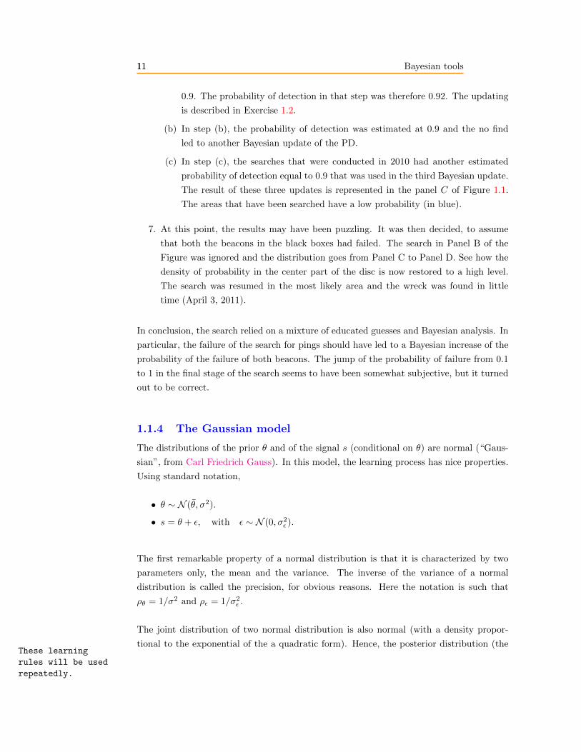
11 Bayesian tools11

0.9. The probability of detection in that step was therefore 0.92. The updating

is described in Exercise 1.2.

(b) In step (b), the probability of detection was estimated at 0.9 and the no find

led to another Bayesian update of the PD.

(c) In step (c), the searches that were conducted in 2010 had another estimated

probability of detection equal to 0.9 that was used in the third Bayesian update.

The result of these three updates is represented in the panel C of Figure 1.1.

The areas that have been searched have a low probability (in blue).

7. At this point, the results may have been puzzling. It was then decided, to assume

that both the beacons in the black boxes had failed. The search in Panel B of the

Figure was ignored and the distribution goes from Panel C to Panel D. See how the

density of probability in the center part of the disc is now restored to a high level.

The search was resumed in the most likely area and the wreck was found in little

time (April 3, 2011).

In conclusion, the search relied on a mixture of educated guesses and Bayesian analysis. In

particular, the failure of the search for pings should have led to a Bayesian increase of the

probability of the failure of both beacons. The jump of the probability of failure from 0.1

to 1 in the final stage of the search seems to have been somewhat subjective, but it turned

out to be correct.

1.1.4 The Gaussian model

The distributions of the prior θ and of the signal s (conditional on θ) are normal (“Gaus-

sian”, from Carl Friedrich Gauss). In this model, the learning process has nice properties.

Using standard notation,

• θ ∼ N (θ, σ2).

• s = θ + ε, with ε ∼ N (0, σ2ε ).

The first remarkable property of a normal distribution is that it is characterized by two

parameters only, the mean and the variance. The inverse of the variance of a normal

distribution is called the precision, for obvious reasons. Here the notation is such that

ρθ = 1/σ2 and ρε = 1/σ2ε .

These learning

rules will be used

repeatedly.

The joint distribution of two normal distribution is also normal (with a density propor-

tional to the exponential of the a quadratic form). Hence, the posterior distribution (the

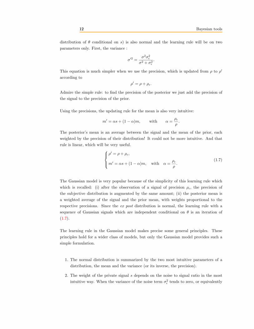
12 Bayesian tools12

distribution of θ conditional on s) is also normal and the learning rule will be on two

parameters only. First, the variance :

σ′2 =σ2σ2

ε

σ2 + σ2ε

.

This equation is much simpler when we use the precision, which is updated from ρ to ρ′

according to

ρ′ = ρ+ ρε.

Admire the simple rule: to find the precision of the posterior we just add the precision of

the signal to the precision of the prior.

Using the precisions, the updating rule for the mean is also very intuitive:

m′ = αs+ (1− α)m, with α =ρερ.

The posterior’s mean is an average between the signal and the mean of the prior, each

weighted by the precision of their distribution! It could not be more intuitive. And that

rule is linear, which will be very useful.ρ′ = ρ+ ρε,

m′ = αs+ (1− α)m, with α =ρερ.

(1.7)

The Gaussian model is very popular because of the simplicity of this learning rule which

which is recalled: (i) after the observation of a signal of precision ρε, the precision of

the subjective distribution is augmented by the same amount; (ii) the posterior mean is

a weighted average of the signal and the prior mean, with weights proportional to the

respective precisions. Since the ex post distribution is normal, the learning rule with a

sequence of Gaussian signals which are independent conditional on θ is an iteration of

(1.7).

The learning rule in the Gaussian model makes precise some general principles. These

principles hold for a wider class of models, but only the Gaussian model provides such a

simple formulation.

1. The normal distribution is summarized by the two most intuitive parameters of a

distribution, the mean and the variance (or its inverse, the precision).

2. The weight of the private signal s depends on the noise to signal ratio in the most

intuitive way. When the variance of the noise term σ2ε tends to zero, or equivalently

13 Bayesian tools13

its precision tends to infinity, the signal’s weight α tends to one and the weight

of the ex ante expected value of θ tends to zero. The expression of α provides a

quantitative formulation of the trivial principle according to which one relies more

on a more precise signal.

3. The signal s contributes to the information on θ which is measured by the increase in

the precision on θ. According to the previous result, the increment is exactly equal to

the precision of the signal (the inverse of the variance of its noise). The contribution of

a set of independent signals is the sum of their precisions. This property is plausible,

but it rules out situations where new information makes an agent less certain about

θ, a point which is discussed further below.

4. More importantly, the increase in the precision on θ is independent of the realization

of the signal s, and can be computed ex ante. This is handy for the measurement

of the information gain which can be expected from a signal. Such a measurement

is essential in deciding whether to receive the signal, either by purchasing it, or by

delaying a profitable investment to wait for the signal.

5. The Gaussian model will fit particularly well with the quadratic payoff function and

the decision problem which will be studied later.

1.1.5 Comparison of the two models

In the binary model, the distinction good/bad state is appealing. The probability distri-

bution is given by one number. The learning rule with the binary signal is simple. These

properties are convenient when solving exercises. The Gaussian model is convenient for

other reasons which were enumerated previously. It is important to realize that each of

the two models embodies some deep properties.

The evolution of confidence

When there are two states, the probability distribution is characterized by the probability

µ of the good state. This value determines an index of confidence: if the two states are 0

and 1, the variance of the distribution is µ(1− µ). Suppose that µ is near 1 and that new

information arrives which reduces the value of µ. This information increases the variance

of the estimate, i.e., it reduces the confidence of the estimate. In the Gaussian model, new

signals cannot reduce the precision of the subjective distribution. They always reduce the

variance of this distribution.

14 Bayesian tools14

Bounded and unbounded private informations

Another major difference between the two models is the strength of the private information.

In the binary model, a signal has a bounded strength. In the updating formula (??),

the multiplier is bounded. (It is either p/(1 − p′) or (1 − p)/p′). When the signal is

symmetric, the parameter p defines its precision. In the Gaussian model, the private signal

is unbounded and the changes of the expected value of θ are unbounded. The boundedness

of a private signal will play an important role in social learning: a bounded private signal

is overwhelmed by a strong prior. (See the example at the beginning of the chapter).

Binary states and Gaussian signals

If we want to represent a situation where confidence may decrease and the private signal

is unbounded, we may turn to a combination of the two previous models.

Assume that the state space Θ has two elements, Θ = {θ0, θ1}, and the private signal is

Gaussian:

s = θ + ε, with ε ∼ N (0, 1/ρ2ε). (1.8)

The LLR is updated according to

λ′ = λ+ ρε(θ1 − θ0)(s− θ1 + θ02

). (1.9)

Since s is unbounded, the private signal has an unbounded impact on the subjective prob-

ability of a state. There are values of s such that the likelihood ratio after receiving s is

arbitrarily large.

1.1.6 Learning may lead to opposite beliefs: polarization

Different people have often different priors. The same information may lead to a conver-

gence or a divergence of their beliefs. Assume first that there are only two states. In this

case, without loss of generality, we can assume that the information takes the form of a

binary signal as in Table 1. If two individuals observe the same signal s, their LR are

multiplied by the same ratio P (s|θ1)/P (s|θ0) that they move in the same direction.

In order to observe diverging updates, there must be more than two states. Consider the

example with three states. these could be that the economy needs a reform to the left

(state 1), to the center (state 2) or to the right (state 3). A signal s is produced either by

a study or the implementation of a particular policy and provides an information on the

state that is represented by the next table. (The signal s = 1 is a strong indication that

15 Bayesian tools15

s = 0 s = 1θ = 1 0.3 0.7θ = 2 0.9 0.1θ = 3 0.3 0.7

the center policy is not working).

Two individuals, Alice and Bob, have their own prior on the states. Alice thinks that a

policy on the right will not work and Bob thinks that a policy on the left will not work.

Both have equal priors between the center and the right or the left. An example is presented

in the next table.

Alice Bob1 0.47 0.062 0.47 0.473 0.06 0.47

Alice Bob1 0.79 0.12 0.11 0.113 0.1 0.79

Priors Posteriors

After the signal s = 1, Alice leans more on the left and Bob more on the right. The signal

generates a polarization For Alice and Bob, the belief in the center decreases and for both

of them, the beliefs in states 1 and 3 increase, but the increase is much higher for the state

that has a higher prior, state 1 for Alice and state 2 for Bob. When θ is measured by a

number, Alice and Bob draw opposite conclusions from the expected value of θ.

16 Bayesian tools16

BIBLIOGRAPHY

* Anderson, Lisa R., and Charles A. Holt (1996). “Understanding Bayes’ Rule,” Journal of

Economic Perspectives, 10(2), 179-187.

Salop, Steven C.. 1987. “Evaluating Uncertain Evidence with Sir Thomas Bayes: A Note

for Teachers,” Journal of Economic Perspectives, 1(1): 155-159.

* Keller, Colleen M. (2015). “Bayesian Search for Missing Aircraft,” slides.

A superb presentation of four famous examples of Bayesian searches by a player in

that field. Highly recommended.

Stone, Lawrence D., Colleen M. Keller, Thomas M. Kratzke and Johan P. Strumprer

(2014). “Search for the Wreckage of Air France Flight AF 447,” Statistical Science, 29 (1),

69-80.

Presents the search for AF 447. The next item, by a member of the team, is a

conference presentation that discusses Bayesian searches for the USS Scorpion, the

USS Central America, AF 447, and the failed search for MH 370. These slides are

highly recommended, especially after reading the relevant section in this chapter.

Dixit, Avinash K. and Jorgen Weibull (2007). “Political polarization,” PNAS, 104 (18),

7351-7356.

Williams, Arlington W., and James M. Walker (1993). “Computerized Laboratory Exer-

cises for Microeconomics Education: Three Applications Motivated by the Methodology

of Experimental Economics,” Journal of Economic Education, 22, 291-315.

Jern, Alan, K-m I. Chang and C. Kemp (2014). “Belief Polarization is not always irra-

tional,” Psychological Review, 121, 206-224.

17 Bayesian tools17

EXERCISE 1.1. (The MLRP)

Construct a signal that does not satisfy the MLRP.

EXERCISE 1.2. (Simple probability computation, searching for a wreck)

An airplane carrying “two blackboxes” crashes into the sea. It is estimated that each box

survives (emits a detectable signal) with probability s. After the crash, a detector is passed

over the area of the crash. (We assume that we are sure that the wreck is in the area).

Previous tests have shown that if a box survives, its signal is captured by the detector with

probability q.

1. Determine algebraically he probability pD that the detector gets a signal. What is

the numerical value of pD for s = 0.8 and q = 0.9?

2. Assume that there are two distinct spots, A and B, where the wreck could be.

Each has a prior probability of 1/2. A detector is flown over the areas. Because of

conditions on the sea floor, it is estimated that if the wreck is in A, the detector finds

it with probability 0.9 while if the wreck is in B, the probability of detection is only

0.5. The search actually produces no detection. What are the ex post probabilities

for finding the wreck in A and B?

EXERCISE 1.3. (non symmetric binary signal)

There are two states of nature, θ0 and θ1 and a binary signal such that P (s = θi|θi) = qi.

Note that q1 and q0 are not equal.

1. Let q1 = 3/4 and q0 = 1/4. Does the signal provide information? In general what is

the condition for the signal to be informative?

2. Find the condition on q1 and q0 such that s = 1 is good news about the state θ1.

EXERCISE 1.4. (Bayes’ rule with a continuum of states)

Assume that an agent undertakes a project which succeeds with probability θ, (fails with

probability 1− θ), where θ is drawn from a uniform distribution on (0, 1).

1. Determine the ex post distribution of θ for the agent after the failure of the project.

2. Assume that the project is repeated and fails n consecutive times. The outcomes are

independent with the same probability θ. Determine an algebraic expression for the

density of θ of this agent. Discuss intuitively the property of this density.