bayesian computation: posterior sampling &...
TRANSCRIPT
Bayesian Computation: Posterior Sampling
& MCMC
Tom LoredoDept. of Astronomy, Cornell University
http://www.astro.cornell.edu/staff/loredo/bayes/
Cosmic Populations @ CASt — 9–10 June 2014
1 / 42

Posterior Sampling & MCMC
1 Posterior sampling
2 Markov chain Monte CarloMarkov chain propertiesMetropolis-Hastings algorithmClasses of proposals
3 MCMC diagnosticsPosterior sample diagnosticsJoint distribution diagnosticsCautionary advice
4 Beyond the basics
2 / 42

Posterior Sampling & MCMC
1 Posterior sampling
2 Markov chain Monte CarloMarkov chain propertiesMetropolis-Hastings algorithmClasses of proposals
3 MCMC diagnosticsPosterior sample diagnosticsJoint distribution diagnosticsCautionary advice
4 Beyond the basics
3 / 42

Posterior sampling
∫
dθ g(θ)p(θ|D) ≈ 1
n
∑
θi∼p(θ|D)
g(θi ) + O(n−1/2)
When p(θ) is a posterior distribution, drawing samples from it iscalled posterior sampling (or simulation from the posterior):
• One set of samples can be used for many different calculations(so long as they don’t depend on low-probability events)
• This is the most promising and general approach for Bayesiancomputation in high dimensions—though with a twist(MCMC!)
Challenge: How to build a RNG that samples from a posterior?
4 / 42

Accept-Reject Algorithm
1 Choose a tractable density h(θ) and a constant C so Ch
bounds q
2 Draw a candidate parameter value θ′ ∼ h
3 Draw a uniform random number, u
4 If q(θ′) < Ch(θ′), record θ′ as a sample
5 Goto 2, repeating as necessary to get the desired number ofsamples.
Efficiency = ratio of volumes, Z/C .
In problems of realistic complexity, the efficiency is intolerably lowfor parameter spaces of more than several dimensions.
Take-away idea: Propose candidates that may be accepted or
rejected
5 / 42

Posterior Sampling & MCMC
1 Posterior sampling
2 Markov chain Monte CarloMarkov chain propertiesMetropolis-Hastings algorithmClasses of proposals
3 MCMC diagnosticsPosterior sample diagnosticsJoint distribution diagnosticsCautionary advice
4 Beyond the basics
6 / 42
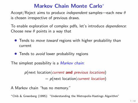
Markov Chain Monte Carlo∗
Accept/Reject aims to produce independent samples—each new θis chosen irrespective of previous draws.
To enable exploration of complex pdfs, let’s introduce dependence:Choose new θ points in a way that
• Tends to move toward regions with higher probability thancurrent
• Tends to avoid lower probability regions
The simplest possibility is a Markov chain:
p(next location|current and previous locations)
= p(next location|current location)
A Markov chain “has no memory.”
∗Chib & Greenberg (1995): “Understanding the Metropolis-Hastings Algorithm”
7 / 42

Markov chain
π(θ)L(θ) contours
θ1
θ2
Initial θ
8 / 42
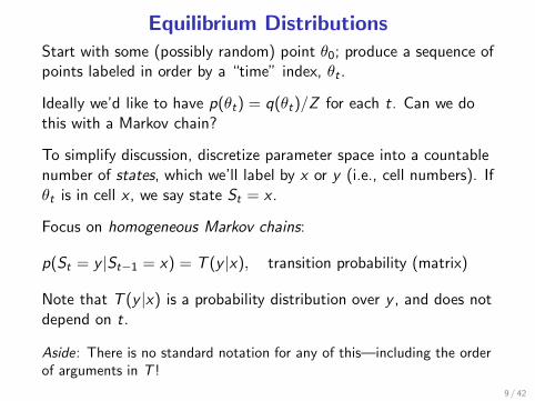
Equilibrium DistributionsStart with some (possibly random) point θ0; produce a sequence ofpoints labeled in order by a “time” index, θt .
Ideally we’d like to have p(θt) = q(θt)/Z for each t. Can we dothis with a Markov chain?
To simplify discussion, discretize parameter space into a countablenumber of states, which we’ll label by x or y (i.e., cell numbers). Ifθt is in cell x , we say state St = x .
Focus on homogeneous Markov chains:
p(St = y |St−1 = x) = T (y |x), transition probability (matrix)
Note that T (y |x) is a probability distribution over y , and does notdepend on t.
Aside: There is no standard notation for any of this—including the orderof arguments in T !
9 / 42

What is the probability for being in state y at time t?
p(St = y) = p(stay at y) + p(move to y)− p(move from y)
= p(St−1 = y)
+∑
x 6=y
p(St−1 = x)T (y |x) −∑
x 6=y
p(St−1 = y)T (x |y)
= p(St−1 = y)
+∑
x 6=y
[p(St−1 = x)T (y |x)− p(St−1 = y)T (x |y)]
If the sum vanishes, then there is an equilibrium distribution:
p(St = y) = p(St−1 = y) ≡ peq(y)
If we start in a state drawn from peq, every subsequent sample willbe a (dependent) draw from peq.
10 / 42

Reversibility/Detailed Balance
A sufficient (but not necessary!) condition for there to be anequilibrium distribution is for each term of the sum to vanish:
peq(x)T (y |x) = peq(y)T (x |y) or
T (y |x)T (x |y) =
peq(y)
peq(x)
the detailed balance or reversibility condition
If we set peq = q/Z , and we build a reversible transitiondistribution for this choice, then the equilibrim distribution will be
the posterior distribution
11 / 42

Convergence
Problem: What about p(S0 = x)?
If we start the chain with a draw from the posterior, everysubsequent draw will be from the posterior. But we can’t do this!
Convergence
If the chain produced by T (y |x) satisifies two conditions:
• It is irreducible: From any x , we can reach any y withfinite probability in a finite # of steps
• It is aperiodic : The transitions never get trapped in cycles
then p(St = s) → peq(x)
Early samples will show evidence of whatever procedure wasused to generate the starting point → discard samples in aninitial “burn-in” period
12 / 42

Designing Reversible TransitionsSet peq(x) = q(x)/Z ; how can we build a T (y |x) with this as itsEQ dist’n?
Steal an idea from accept/reject: Start with a proposal orcandidate distribution, k(y |x). Devise an accept/reject criterionthat leads to a reversible T (y |x) for q/Z .
Using any k(y |x) as T will not guarantee reversibility. E.g., from aparticular x , the transition rate to a particular y may be too large:
q(x)k(y |x) > q(y)k(x |y) Note: Z dropped out!
When this is true, we should use rejections to reduce the rate to y .
Acceptance probability : Accept y with probability α(y |x); reject itwith probability 1− α(y |x) and stay at x :
T (y |x) = k(y |x)α(y |x) + [1− α(y |x)]δy ,x
13 / 42

The detailed balance condition is a requirement for y 6= x
transitions, for which δy ,x = 0; it gives a condition for α:
q(x)k(y |x)α(y |x) = q(y)k(x |y)α(x |y)
Suppose q(x)k(y |x) > q(y)k(x |y); then we want to suppressx → y transitions, but we want to maximize y → x transitions. Sowe should set α(x |y) = 1, and the condition becomes:
α(y |x) = q(y)k(x |y)q(x)k(y |x)
If instead q(x)k(y |x) < q(y)k(x |y), the situation is reversed: wewant α(y |x) = 1, and α(x |y) should suppress y → x transitions
14 / 42
We can summarize the two cases as:
α(y |x) ={
q(y)k(x |y)q(x)k(y |x) if q(y)k(x |y) < q(x)k(y |x)1 otherwise
or equivalently:
α(y |x) = min
[
q(y)k(x |y)q(x)k(y |x) , 1
]
15 / 42

Metropolis-Hastings algorithm
Given a target quasi-distribution q(x) (it need not be normalized):
1. Specify a proposal distribution k(y |x) (make sure it isirreducible and aperiodic).
2. Choose a starting point x ; set t = 0 and St = x
3. Increment t4. Propose a new state y ∼ k(y |x)5. If q(x)k(y |x) < q(y)k(x |y), set St = y ; goto (3)6. Draw a uniform random number u7. If u < q(y)k(x|y)
q(x)k(y|x) , set St = y ; else set St = x ; goto (3)
The art of MCMC is in specifying the proposal distribution k(y |x)
We want:
• New proposals to be accepted, so there is movement• Movement to be significant, so we explore efficiently
These desiderata compete!
16 / 42

Random walk Metropolis (RWM)Propose an increment, z , from the current location, not dependenton the current location, so y = x + z with a specified PDF K (z),corresponding to
k(y |x) = K (y − x)
The proposals would give rise to a random walk if they were allaccepted; the M-H rule modifies them to be a kind of directedrandom walk
Most commonly, a symmetric proposal is adopted:
k(y |x) = K (|y − x |)
The acceptance probability simplifies:
α(y |x) = min
[
q(y)
q(x), 1
]
Key issues: shape and scale (in all directions) of K (z)17 / 42

RWM in 2-D
MacKay (2003)
Small step size → good acceptance rate, but slow exploration
18 / 42

Independent Metropolis (IM)
Propose a new point independently of the current location:
k(y |x) = K (y)
The acceptance probability is now
α(y |x) = min
[
q(y)K (x)
q(x)K (y), 1
]
Note if K (·) ∝ q(·), proposals are from the target and are alwaysaccepted
Good acceptance requires K (·) to resemble the posterior → IM istypically only useful in low-D problems where we can construct agood K (·) (e.g., MVN at the mode)
19 / 42

Blocking and Gibbs samplingBasic idea: Propose moves of only subsets of the parameters at atime in an effort to improve rate of exploration
Suppose x = (x1, x2) is 2-D. If we alternate two 1-D M-H samplers,
• Targeting peq(x1) ∝ p(x1|x2)
• Targeting peq(x2) ∝ p(x2|x1)
then the resulting chain produces samples from p(x)
The simplest case is Gibbs sampling, which alternates proposalsdrawn directly from full conditionals:
p(x1|x2) =p(x1, x2)
p(x2)∝ p(x1, x2) with x2 fixed
p(x2|x1) =p(x1, x2)
p(x1)∝ p(x1, x2) with x1 fixed
M-H with these proposals always accepts20 / 42

Gibbs sampling in 2-D
MacKay (2003)
21 / 42
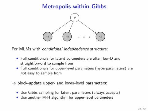
Metropolis-within-Gibbs
θ
x1 x2 xN
For MLMs with conditional independence structure:
• Full conditionals for latent parameters are often low-D andstraightforward to sample from
• Full conditionals for upper-level parameters (hyperparameters) arenot easy to sample from
⇒ block-update upper- and lower-level parameters:
• Use Gibbs sampling for latent parameters (always accepts)• Use another M-H algorithm for upper-level parameters
22 / 42
Posterior Sampling & MCMC
1 Posterior sampling
2 Markov chain Monte CarloMarkov chain propertiesMetropolis-Hastings algorithmClasses of proposals
3 MCMC diagnosticsPosterior sample diagnosticsJoint distribution diagnosticsCautionary advice
4 Beyond the basics
23 / 42

The Good NewsThe Metropolis-Hastings algorithm enables us to draw a few timeseries realizations {θt}, t = 0 to N, from a Markov chain with aspecified stationary distribution p(θ)
The algorithm works for any f (θ) ∝ p(θ), i.e., Z needn’t be known
The marginal distribution at each time is pt(θ)
• Stationarity: If p0(θ) = p(θ), then pt(θ) = p(θ)
• Convergence: If p0(θ) 6= p(θ), eventually
||pt(θ), p(θ)|| < ǫ
for an appropriate norm between distributions
• Ergodicity:
g ≡ 1
N
∑
i
g(θi ) → 〈g〉 ≡∫
dθ g(θ)p(θ)
24 / 42
The Bad News
• We never have p0(θ) = p(θ): we have to figure out how toinitialize a realization, and we are always in the situationwhere pt(θ) 6= p(θ)
• “Eventually” means t < ∞; that’s not very comforting!
• After convergence at time t = c , pt(θ) ≈ p(θ), but θ valuesat different times are dependent; the Markov chain CLT says
g ∼ N(〈g〉, σ2/N)
σ2 = var[g(θc )] + 2∞∑
k=1
cov[g(θc ), g(θc+k )]
• We have to learn about pt(θ) from just a few time seriesrealizations (maybe just one)
25 / 42

Posterior sample diagnosticsPosterior sample diagnostics use single or multiple chains, {θt}, todiagnose:
• Convergence: How long until starting values are forgotten?(Discard as “burn-in,” or run long enough so averages“forget” initialization bias.)
• Mixing: How long until we have fairly sampled the fullposterior? (Make finite-sample Monte Carlo uncertaintiessmall.)
Two excellent R packages with routines, descriptions, references:
• boahttp://cran.r-project.org/web/packages/boa/index.html
• codahttp://cran.r-project.org/web/packages/coda/index.html
They also supply other output analyses: estimating means,variances, marginals, HPD regions. . .
26 / 42
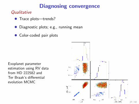
Diagnosing convergenceQualitative
• Trace plots—trends?
• Diagnostic plots; e.g., running mean
• Color-coded pair plots
Exoplanet parameterestimation using RV datafrom HD 222582 andTer Braak’s differentialevolution MCMC
27 / 42
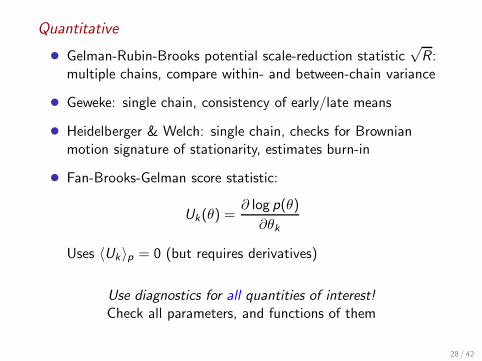
Quantitative
• Gelman-Rubin-Brooks potential scale-reduction statistic√R:
multiple chains, compare within- and between-chain variance
• Geweke: single chain, consistency of early/late means
• Heidelberger & Welch: single chain, checks for Brownianmotion signature of stationarity, estimates burn-in
• Fan-Brooks-Gelman score statistic:
Uk(θ) =∂ log p(θ)
∂θk
Uses 〈Uk〉p = 0 (but requires derivatives)
Use diagnostics for all quantities of interest!
Check all parameters, and functions of them
28 / 42
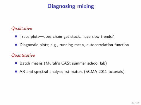
Diagnosing mixing
Qualitative
• Trace plots—does chain get stuck, have slow trends?
• Diagnostic plots; e.g., running mean, autocorrelation function
Quantitative
• Batch means (Murali’s CASt summer school lab)
• AR and spectral analysis estimators (SCMA 2011 tutorials)
29 / 42
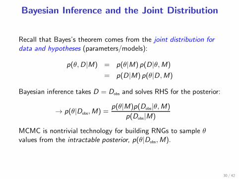
Bayesian Inference and the Joint Distribution
Recall that Bayes’s theorem comes from the joint distribution for
data and hypotheses (parameters/models):
p(θ,D|M) = p(θ|M) p(D|θ,M)
= p(D|M) p(θ|D,M)
Bayesian inference takes D = Dobs and solves RHS for the posterior:
→ p(θ|Dobs,M) =p(θ|M)p(Dobs|θ,M)
p(Dobs|M)
MCMC is nontrivial technology for building RNGs to sample θvalues from the intractable posterior, p(θ|Dobs,M).
30 / 42

Posterior sampling is hard, but sampling from the otherdistributions is often easy:
• Often easy to draw θ∗ from π(θ)
• Typically easy to draw Dsim from p(D|θ,M)
• Thus we can sample the joint for (θ,D) by sequencing:
θ∗ ∼ π(θ)
Dsim ∼ p(D|θ∗,M)
• {Dsim} from above are samples from prior predictive,
p(D|M) =
∫
dθ π(θ)p(D|θ,M)
Now note that {Dsim, θ} with θ ∼ p(θ|Dsim,M) are also samplesfrom the joint distribution
Joint distribution methods check the consistency of these two jointsamplers to validate a posterior sampler
31 / 42

Example: “Calibration” of credible regions
How often may we expect an HPD region with probability P toinclude the true value if we analyze many datasets? I.e., what’s thefrequentist coverage of an interval rule ∆(D) defined bycalculating the Bayesian HPD region each time?
Suppose we generate datasets by picking a parameter value fromπ(θ) and simulating data from p(D|θ).
The fraction of time θ will be in the HPD region is:
Q =
∫
dθ π(θ)
∫
dD p(D|θ) Jθ ∈ ∆(D)K
Note π(θ)p(D|θ) = p(θ,D) = p(D)p(θ|D), so
Q =
∫
dD
∫
dθ p(θ|D) p(D) Jθ ∈ ∆(D)K
32 / 42

Q =
∫
dD
∫
dθ p(θ|D) p(D) Jθ ∈ ∆(D)K
=
∫
dD p(D)
∫
dθ p(θ|D) Jθ ∈ ∆(D)K
=
∫
dD p(D)
∫
∆(D)dθ p(θ|D)
=
∫
dD p(D)P
= P
The HPD region includes the true parameters 100P% of the time
This is exactly true for any problem, even for small datasets
Keep in mind it involves drawing θ from the prior; credible regionsare “calibrated with respect to the prior”
33 / 42

A Tangent: Average Coverage
Recall the original Q integral:
Q =
∫
dθ π(θ)
∫
dD p(D|θ) Jθ ∈ ∆(D)K
=
∫
dθ π(θ)C (θ)
where C (θ) is the (frequentist) coverage of the HPD region whenthe data are generated using θ
This indicates Bayesian regions have accurate average coverage
The prior can be interpreted as quantifying how much we careabout coverage in different parts of the parameter space
34 / 42

Basic Bayesian Calibration Diagnostics
Encapsulate your sampler: Create an MCMC posterior samplingalgorithm for model M that takes data D as input and producesposterior samples {θi}, and a 100P% credible region ∆P(D)
Initialize counter Q = 0Repeat N ≫ 1 times:
1 Sample a “true” parameter value θ∗ from π(θ)
2 Sample a dataset Dsim from p(D|θ∗)3 Use the encapsulated posterior sampler to get ∆P(Dsim) from
p(θ|Dsim,M)
4 If θ∗ ∈ ∆P(D), increment Q
Check that Q/N ≈ P
35 / 42

Easily extend the idea to check all credible region sizes:
Initialize a list that will store N probabilities, PRepeat N ≫ 1 times:
1 Sample a “true” parameter value θ∗ from π(θ)
2 Sample a dataset Dsim from p(D|θ∗)3 Use the encapsulated posterior sampler to get {θi} from
p(θ|Dsim,M)
4 Find P so that θ∗ is on the boundary of ∆P(D); append to list[P = fraction of {θi} with q(θi ) > q(θ∗)]
Check that the Ps follow a uniform distribution on [0, 1]
36 / 42

Other Joint Distribution Tests
• Geweke 2004: Calculate means of scalar functions of (θ,D)two ways; compare with z statistics
• Cook, Gelman, Rubin 2006: Posterior quantile test, expectp[g(θ) > g(θ∗)] ∼ Uniform (HPD test is special case)
37 / 42

What Joint Distribution Tests AccomplishSuppose the prior and sampling distribution samplers arewell-validated
• Convergence verification: If your sampler is bug-free butwas not run long enough → unlikely that inferences will becalibrated
• Bug detection: An incorrect posterior samplerimplementation will not converge to the correct posteriordistribution → unlikely that inferences will be calibrated, evenif the chain converges
Cost: Prior and data sampling is often cheap, but posteriorsampling is often expensive, and joint distribution tests require yourun your MCMC code hundreds of times
Compromise: If MCMC cost grows with dataset size, running thetest with smaller datasets provides a good bug test, and some
insight on convergence38 / 42
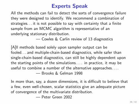
Experts SpeakAll the methods can fail to detect the sorts of convergence failurethey were designed to identify. We recommend a combination ofstrategies. . . it is not possible to say with certainty that a finitesample from an MCMC algorithm is representative of anunderlying stationary distribution.
— Cowles & Carlin review of 13 diagnostics
[A]ll methods based solely upon sampler output can befooled. . . and multiple-chain-based diagnostics, while safer thansingle-chain-based diagnostics, can still be highly dependent uponthe starting points of the simulations. . . . in practice, it may beuseful to combine a number of the alternative approaches. . . .
— Brooks & Gelman 1998
In more than, say, a dozen dimensions, it is difficult to believe thata few, even well-chosen, scalar statistics give an adequate pictureof convergence of the multivariate distribution.
— Peter Green 200239 / 42
Handbook of Markov Chain Monte Carlo (2011)
Your humble author has a dictum that the least one can do is to
make an overnight run. What better way for your computer tospend its time? In many problems that are not too complicated,this is millions or billions of iterations. If you do not make runs like
that, you are simply not serious about MCMC. Your humble authorhas another dictum (only slightly facetious) that one should start arun when the paper is submitted and keep running until thereferees’ reports arrive. This cannot delay the paper, and maydetect pseudo-convergence.
— Charles Geyer
When all is done, compare inferences to those from simpler modelsor approximations. Examine discrepancies to see whether theyrepresent programming errors, poor convergence, or actual changesin inferences as the model is expanded.
— Gelman & Shirley
40 / 42

Posterior Sampling & MCMC
1 Posterior sampling
2 Markov chain Monte CarloMarkov chain propertiesMetropolis-Hastings algorithmClasses of proposals
3 MCMC diagnosticsPosterior sample diagnosticsJoint distribution diagnosticsCautionary advice
4 Beyond the basics
41 / 42

Much More to Computational BayesFancier MCMC• Sophisticated proposals (e.g., with auxiliary variables)
• Adaptive proposals (use many past states)
• Population-based MCMC (e.g., differential evolution MCMC)
Sequential Monte Carlo• Particle filters for dynamical models (posterior tracks a changing
state)
• Adaptive importance sampling (“evolve” posterior via annealing oron-line processing)
Model uncertainty• Marginal likelihood computation: Thermodynamic integration,
bridge sampling, nested sampling
• MCMC in model space: Reversible jump MCMC, birth/death
• Exploration of large (discrete) model spaces (e.g., variableselection): Shotgun stochastic search, Bayesian adaptive sampling
This is just a small sampling!42 / 42