bayesian approach for fatigue life prediction from field ... · bayesian approach for fatigue life...

Bayesian Approach for Fatigue Life Prediction from Field Inspection

Dawn An, and Jooho Choi School of Aerospace & Mechanical Engineering, Korea Aerospace University

[email protected], [email protected]

Nam H. Kim, and Sriram Pattabhiraman Dept. of Mechanical & Aerospace Engineering, University of Florida

[email protected], [email protected]

Abstract: In the design considering fatigue life of mechanical components, uncertainties arising from the materials and manufacturing processes should be taken into account for ensuring reliability. Common practice in the design is to apply safety factor in conjunction with the numerical codes for evaluating the lifetime. This approach, however, most likely relies on the designer's experience. Besides, the predictions often are not in agreement with the real observations during the actual use. In this paper, a more dependable approach based on the Bayesian technique is proposed, which incorporates the field failure data with the prior knowledge to obtain the posterior distribution of the unknown parameters of the fatigue life. A matter of prior knowledge is also considered since the posterior distribution is influenced by it. Posterior predictive distributions and associated values are estimated afterwards, which represents the degree of our belief of the life conditional on the observed data. As more data are provided, the values will be updated to more confident information. The results can be used in various needs such as a risk analysis, reliability based design optimization, maintenance scheduling, or validation of reliability analysis codes. In order to obtain the posterior distribution, Markov Chain Monte Carlo (MCMC) technique is employed, which is a modern statistical computational method which draws effectively the samples of the given distribution. Field data of turbine components are exploited to illustrate our approach, which counts as a regular inspection of the number of failed blades in a turbine disk.

Keywords: Fatigue life, Prior distribution, Posterior distribution, Bayesian approach, Markov Chain Monte Carlo Technique, Field Inspection, Turbine blade

1. Introduction

Performance of mechanical components undergoes a change by uncertainties such as environmental effects, dimensional tolerances, loading conditions, material properties and maintenance processes. Fatigue lives of the components in particular are significantly influenced even by small changes. In the design for fatigue life, it is not feasible to consider all the uncertainties of the relevant variables, since most of them are not characterized in the design phase. Analytical prediction of fatigue life is therefore, often not in agreement with the field data. Common practice in the design is then to apply proper “safety factor” when evaluating fatigue life. This approach, however, causes overdesign or risk of design, since it relies on the designer’s experience. Recently, for more reliable life prediction, the study using field data have been undertaken (Marahleh et al., 2006). Field data can be helpful in predicting fatigue life that has uncertainties due to the

4th International Workshop on Reliable Engineering Computing (REC 2010)Edited by Michael Beer, Rafi L. Muhanna and Robert L. MullenCopyright © 2010 Professional Activities Centre, National University of Singapore.ISBN: 978-981-08-5118-7. Published by Research Publishing Services.doi:10.3850/978-981-08-5118-7 043

614

Dawn An, Jooho Choi, Nam H. Kim, and Sriram Pattabhiraman

unknown potential inputs. This approach can be dealt with Bayesian technique which incorporates the field failure data with the prior knowledge to obtain the posterior distribution of the unknown parameters of the fatigue life (Kim et al., 2009). As more data are provided, the values will be updated to more confident information. In this paper, Markov Chain Monte Carlo (MCMC) technique is employed as an efficient means to draw samples of given distribution (Andrieu et al., 2003). Consequently, the posterior distribution of the unknown parameters of the fatigue life is obtained in light of the field data collected from the inspection of turbine blades. Subsequently, fatigue life of turbine blades is predicted a posteriori based on the drawn samples.

2. Bayesian Technique for Lifetime Prediction

Bayesian technique is employed to update lifetime prediction using analytical model and field data, which is based on Bayes’ rule and defined as (Gelman et al., 2004) :

| |f L fD D (1)

where |L D is the likelihood of observed data , ,D t y n conditional on the given model parameters

(in the case of normal distribution, are the mean and standard deviation ), f is the prior

distribution of , and |f D is posterior distribution of conditional on the D . The procedure to obtain

posterior distribution |f D is outlined as follows.

In Eq.(1), likelihood is just a multiplication of each binomial PDF, given as

1

| Bin | ,Di

N

i i f

i

L y n p (2)

where life0

|i

i

t

fp f t dt (3)

and , , ,i i iN t y n are given in the Table I which is a field data for inspected turbine blades. In the case of the

first inspection, we found 2 failures out of 40 blades at the time of 4321 hours and N is 13 which is set of

inspected data. In Eq.(3), life |f t denotes PDF of lifetime of turbine blade, which can be assumed to a

certain predetermined model, which is in this paper, a normal distribution or weibull distribution.

Consequently, the posterior PDF in Eq. (1) is obtained by multiplicatying Eq. (2) and the prior PDF f .

Table I. Field data for inspected turbine blades

Engine Hours( it ) Failed( iy )/Total( in ) Engine Hours( it ) Failed( iy )/Total( in )

1 4321 2/40 8 1456 0/40

2 3125 1/40 9 26123 13/40

3 1500 1/40 10 3654 0/40

4 9152 0/40 11 8541 0/40

5 12000 12/40 12 6542 10/40

6 11654 3/40 13( N ) 18687 18/40

7 6011 6/40

4th International Workshop on Reliable Engineering Computing (REC 2010) 615


In this paper, the PDF of lifetime life |f t and the prior PDF f are assumed as the following cases:

case 1. life |f t : normal dist. and f : non-informative prior (4)

case 2. life |f t : normal dist. and , 5169,5169 / 2 794,794 / 2f N N (5)

case 3. life |f t : normal dist. and 2, 8030,8030 / 5 40f N (6)

case 4. life | ,f t m : Weibull dist. and , 8.55,0.1 6.67,0.1f m LogN LogN (7)

In terms of the likelihood, normal and Weibull distribution are considered. In the model, the associated model parameters are in the case of normal and ,m in the case of Weibull distribution, respectively.

These are taken to be unknown and are estimated using the inspected data. In the Weibull distribution, ,m

denote scale and shape parameter, respectively. In terms of prior, four cases are considered to examine the effects of prior knowledge on the posterior PDF of model parameters and predicted lifetime of turbine blades. If there is specific prior information, models like the cases 2, 3, 4 can be provided. Otherwise, non-informative prior like the case 1 is used.

The results of case 1 where the likelihood is normal distribution and non-informative prior are shown in Figure 1. In Figure 1(a), the contours of joint posterior PDF of the unknown parameters are plotted. In these figures, the updated prior and the likelihood are obtained from the posterior distribution previously obtained and the inspection data, respectively. The posterior distribution is obtained by multiplying the prior and likelihood, and is used in the next updating step as the prior distribution. In Figure 1(b) and (c), posterior PDF are plotted again in the form of contour and 3D shape respectively. It is shown that as more data are added, the location and range of , moves and narrows down to converge to a certain point. The results

indicate our knowledge on the unknown parameters based on the field inspection.

using only the1st data

0 2 4 6 8 10

1

2

3

4

5

6using 1st~4th data

0 2 4 6 8 10

1

2

3

4

5

6

from field data

updated prior

posterior

using 1st~7th data

0 2 4 6 8 10

1

2

3

4

5

6

updated prior

posterior

from field data

using 1st~10th data

0 2 4 6 8 10

1

2

3

4

5

6

posterior

updated prior

from field data

using 1st~13th data

0 2 4 6 8 10

1

2

3

4

5

6

posterior

updated prior

from field data

(a) likelihood function and updated prior and posterior distribution


0 2 4 6 8 10

1

2

3

4

5

6using 1st~4th data

0 2 4 6 8 10

1

2

3

4

5

6using 1st~7th data

0 2 4 6 8 10

1

2

3

4

5

6using 1st~10th data

0 2 4 6 8 10

1

2

3

4

5

6using 1st~13th data

0 2 4 6 8 10

1

2

3

4

5

6

(b) contour of joint posterior PDF

616 4th International Workshop on Reliable Engineering Computing (REC 2010)


(c) 3-D plot of joint posterior PDFFigure 1. Updated posterior PDF of case 1.

The results of case 2~4 are shown in Figure 2. The results of case 2 where the likelihood is still normal distribution but with normally distributed priors are shown in Figure 2(a) and (b). The figure 2(b) shows the convergent behavior on the two parameters as we collect more and more da a. The results of case 3 where the likelihood is normal and the prior for the sigma is changed to chi-square distribution, which is more reasonable assumption due to the non-negativity, are shown in Figure 2(c) and (d). The results of case 4 where the likelihood is Weibull and the priors are lognormal are shown in Figure 2(e) and (f). The Figure 2(f) shows again the convergent behavior. This case is the most reasonable because the Weibull distribution is the best model for the lifetime.


0 2 4 6 8 10

0.5

1

1.5

2

2.5

3

3.5

4

4.5

5

5.5

6

priorfrom field data

posterior

posterior dist. contour

0 0.5 1 1.5 2 2.5 3 3.5 4

0.2

0.4

0.6

0.8

1

1.2

1.4

1st~4th data

only 1st data

1st~7th data

1st~10th data

1st~13th data

(a) the results using only the 1st data of case 2 (b) updated posterior PDF contours of case 2


0 0.5 1 1.5 2 2.5

0.05

0.1

0.15

0.2

0.25

0.3

0.35

0.4

0.45

0.5

posterior

prior

from field data


0 0.5 1 1.5 2 2.5

0.05

0.1

0.15

0.2

0.25

0.3

0.35

0.4

0.45

0.5

only 1st data

1st~4th data

1st~7th data

1st~10th data

1st~13th data

(c) the results using only the 1st data of case 3 (d) updated posterior PDF contours of case 3



m(shape parameter)

(sca

le p

aram

eter

)


1 2 3 4 5 6 7 8 9

0.2

0.4

0.6

0.8

1

1.2

1.4

1.6

1.8

prior

from field dataposterior

m(shape parameter)

(sca

le p

aram

eter

)


1 2 3 4 5 6 7 8 9

0.2

0.4

0.6

0.8

1

1.2

1.4

1.6

1.8

1st~10th data

1st~13th data

1st~7th data

1st~4th dataonly 1st data

(e) the results using only the 1st data of case 4 (f) updated posterior PDF contours of case 4 Figure 2. Updated posterior PDF of case 2~4.

The final updated results of all cases are shown in Figure 3. The Figure 3(a) and (b) are the results of

and of the normal distribution and m and of the weibull distribution, respectively. Case 1 in Figure

3(a) and the joint PDF on the right in Figure 3(b) are the results of the non-informative priors. As was expected, the results are much wider than the others due to the non-information of the prior. If there is specific prior information, the precision of the posterior distribution is increased.

posterior dist. contour (likeli-N)

0 1 2 3 4 5 6 7

0.5

1

1.5

2

2.5

3

3.5

4

4.5

case 1

case 3case 2

m(shape parameter)

(sca

le p

aram

eter

)posterior dist. contour (likeli-W)

1 2 3 4 5 6 7 8 9

0.2

0.4

0.6

0.8

1

1.2

1.4

1.6

1.8

case 4. using prior

non-informative(in case 4)

(a) likelihood is normal distribution (b) likelihood is weibull distribution Figure 3. Final updated results of all cases.

3. Posterior Distribution using MCMC

3.1. MCMC SIMULATION

Once the expression for posterior PDF is available, one can proceed to sample from the PDF. Primitive way is to compute the values at a grid of points after identifying the effective range, and sample by inverse CDF method. The method, however, has several drawbacks such as the difficulty finding correct location and scale of the grid points, spacing of the grid, and so on. MCMC simulation is an effective solution in this case (Andrieu et al., 2003). The Metropolis-Hastings (M-H) algorithm is typical method of MCMC, which is given in the case of a single parameter by the following procedure:



(0)

0,1

* *

* *

*

*

1 *

1. Initialise .

2. For 0 to 1

Sample ~ .

Sample ~ | .

| if , min 1,

|

else

i

i

i

i i

i

i

x

i N

u U

x q x x

p x q x xu A x x

p x q x x

x x

x1 i

x

(8)

where 0

x is the initial value of an unknown parameter to estimate, N is the number of iterations or

samples, U is the uniform distribution, p x is the posterior PDF (target PDF), and q x is an arbitrary

chosen proposal distribution. A uniform distribution is used in this study for the sake of simplicity. Then, *|

iq x x and * |

iq x x become constant, and q x can be ignored. As an example of MCMC, in Figure

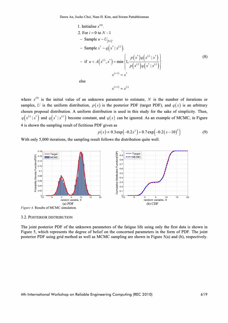
4 is shown the sampling result of fictitious PDF given as 220.3exp 0.2 0.7exp 0.2 10p x x x (9)

With only 5,000 iterations, the sampling result follows the distribution quite well.

-10 -5 0 5 10 15 200

0.02

0.04

0.06

0.08

0.1

0.12

0.14

0.16

0.18

random variable, X

Pro

bab

ility

De

nsi

ty F

unc

tion

(PD

F) Target

MCMC

-10 -5 0 5 10 15 200

0.1

0.2

0.3

0.4

0.5

0.6

0.7

0.8

0.9

1

random variable, X

Cum

ulat

ive

Dis

trib

utio

n F

unct

ion(

CD

F)

TargetMCMC

(a) PDF (b) CDF Figure 4. Results of MCMC simulation.

3.2. POSTERIOR DISTRIBUTION

The joint posterior PDF of the unknown parameters of the fatigue life using only the first data is shown in Figure 5, which represents the degree of belief on the concerned parameters in the form of PDF. The joint posterior PDF using grid method as well as MCMC sampling are shown in Figure 5(a) and (b), respectively.



In Table II, statistical moments by the two methods are compared. As shown in the table, the two methods agree quite closely but MCMC used 10(10)3 samples, whereas gird used 250(10)3 samples.

(a) using grid method (500 500 grid) (b) using MCMC (104 iterations)

Figure 5. Joint posterior PDF of case 2.

Table II. Statistical moments by the two methods

E E E E E

Grid 1.1476 0.1854 0.0160 0.0043 -0.0000

MCMC 1.1498 0.1857 0.0178 0.0048 0.0000

4. Posterior Predictive Distribution

The drawn samples of the parameters obtained in section 3 are used for predicting the failure probability. The initially given prior and final updated posterior predictive distributions of fatigue life are shown in Figure 6. Due to the uncertainties of the model parameters, we have a CDF in a confidence bands. In the figure, dotted and solid curve denote initial and final CDF respectively. Black, red and magenta colors denote median, 5% lower bound and 95% upper bound of the CDF at each stage respectively. I order to accommodate safety, it is advised to take 5% lower bound of the CDF which is colored as red. In Figure 6(a), which is the result of case 1, CDF of fatigue life after the final update is located to the left of the previous one, which reflects the

field data depicted as blue star in more suitable manner. In Figure 6(b) (c), however, the results are found

differently, i.e., the CDF after the final update is located to the right of the initial one in spite of added field data. The reason might be attributed to the wrong information of the priors. In Figure 6(d), the CDF of fatigue life after the final update is located to the left of the initial one below the B10 life, which is the part of our interests. In Figure 6(e), the CDFs of the four cases at 5% lower bound are plotted together. From the figure, it is found that the CDF of the case4 is the most reasonable one because the CDF is overall located to the left of the field data.

From the results, confidence interval of the 1% life and 10% life, which are also called B1 life and B10 life, are given in Table III. In the cases 1 and 3, which employed normal model, we have negative values for the life, which was due to the wrong assumption of the model. On the other hand, the case 4 is the reasonable



model as mentioned before, which shows the positive values. In case that we are ignorant of the type of the distribution, it is advised to choose the most conservative one, which is the case 4 in this study.

0 1 2 3 4 5 6 7 8

x 104

0

0.1

0.2

0.3

0.4

0.5

0.6

0.7

0.8

0.9

1

Operation Hours

CD

F

median5% lower bound95% upper boundfield data

1st~9th data

final

0 1 2 3 4 5 6 7 8

x 104

0

0.1

0.2

0.3

0.4

0.5

0.6

0.7

0.8

0.9

1

Operation Hours

CD

F


final

initial

0 1 2 3 4 5 6 7 8

x 104

0

0.1

0.2

0.3

0.4

0.5

0.6

0.7

0.8

0.9

1

Operation Hours

CD

F


final

initial

(a) case 1 (b) case 2 (c) case 3

0 1 2 3 4 5 6 7 8

x 104

0

0.1

0.2

0.3

0.4

0.5

0.6

0.7

0.8

0.9

1

Operation Hours

CD

F

median5% lower bound95% upper boundfeild data

initial

final

0 1 2 3 4 5 6 7 8

x 104

0

0.1

0.2

0.3

0.4

0.5

0.6

0.7

0.8

0.9

1

Operation Hours

CD

Fcase 1case 2case 3case 4field data

(d) case 4 (e) merged results of all cases Figure 6. Final updated distribution of fatigue life.

Table III. Confidence interval of fatigue life

case 1 case 2 case 3 case 4

5% lower 95% upper 5% lower 95% upper 5% lower 95% upper 5% lower 95% upper

1% Pf -13,836 -4,099 3,988 6,053 -3,774 -76 205 544

10% Pf 6,207 10,361 9,980 11,726 4,934 7,321 2,270 3,711

5. Conclusions

In this paper, a Bayesian updating technique is presented, which incorporates the statistical prediction with field data. By using MCMC simulation, samples of model parameters ( , or ,m ) are drawn

effectively, which are parameters of the fatigue life distribution. After getting samples for joint posterior PDF of , the fatigue life prediction results are obtained, which have a CDF in a confidence bands due to the uncertainties of the model parameters. If there is specific prior information of model parameters, the



precision of the posterior distribution is increased. Caution should be paid, however, that if the prior information is wrong, the result is worse than the one with non-information as was evidenced in the case study. By using the adequate prior with proved accuracy, reliability is improved as the number of field data increase. In case that the type of the distribution of the likelihood is not known a priori, it is advised to choose the most conservative one after examining several candidates as was found in this study.

Acknowledgements

This research was supported by Basic Science Research Program Through the National Research Foundation of Korea (NRF) funded by the Ministry of Education, Science and Technology (2008-02-010 and 2009-0081438)

References

Andrieu, C., N. de Freitas, A. Doucet, and M. Jordan. An introduction to MCMC for Machine Learning. Machine Learning, 50:5-43, 2003.

Gelman, A., J. B. Carlim, H. S. Stern, and D. B. Rubin. Bayesian Data Analysis (second ed.). New York, Chapman & Hall/CRC, 2004.

Kim, N. H., S. Pattabhiraman, and L.A. Houck III. Bayesian Technique for Incorporating Field Experience into Analytical Model for Life Predictions. ASME International Mechanical Engineering Congress and Exposition, Lake Buena Vista, Florida, November, 2009.

Marahleh, G., A. R. I. Kheder, and H. F. Hamad. Creep-Life Prediction of Service-Exposed Turbine Blades. Materials

Science, 42(4), 2006.


bayesian approach for fatigue life prediction from field ... · bayesian approach for fatigue life...

Documents